MURANA: A Generic Framework for
Stochastic Variance-Reduced Optimization

Abstract

We propose a generic variance-reduced algorithm, which we call MUltiple RANdomized Algorithm (MURANA), for minimizing a sum of several smooth functions plus a regularizer, in a sequential or distributed manner. Our method is formulated with general stochastic operators, which allow us to model various strategies for reducing the computational complexity. For example, MURANA supports sparse activation of the gradients, and also reduction of the communication load via compression of the update vectors. This versatility allows MURANA to cover many existing randomization mechanisms within a unified framework, which also makes it possible to design new methods as special cases.

1 Introduction

We consider the estimation of the model $x^{\star}\in\mathbb{R}^{d}$, for some $d\geq 1$, arising as the solution of the optimization problem

$$\operatorname*{minimize}_{x\in\mathbb{R}^{d}}\left(R(x)+\frac{1}{M}\sum_{m=1}^{M}F_{m}(x)\right),$$ (1)

for some $M\geq 1$, where each convex function $F_{m}$ is $L$-smooth, for some $L>0$, i.e. $\frac{1}{L}\nabla F_{m}$ is nonexpansive, and $R:\mathbb{R}^{d}\rightarrow\mathbb{R}\cup\{+\infty\}$ is a proper, closed, convex function (Bauschke and Combettes, 2017), whose proximity operator

$$\mathrm{prox}_{\gamma R}:w\mapsto\operatorname*{arg\,min}_{x\in\mathbb{R}^{d}}\left(\gamma R(x)+\frac{1}{2}\left\|x-w\right\|^{2}\right)$$

is easy to compute, for any $\gamma>0$ (Parikh and Boyd, 2014; Condat et al., 2022a). We introduce

$$F\coloneqq\frac{1}{M}\sum_{m=1}^{M}F_{m}$$

and we suppose that $F$ is $\mu$-strongly convex, for some $\mu>0$, i.e. $F-\frac{\mu}{2}\left\|\cdot\right\|^{2}$ is convex. Since the problem (1) is strongly convex, $x^{\star}$ exists and is unique.

In a distributed client-server setting, $M$ is the number of parallel computing nodes, with an additional master node communicating with these $M$ nodes. Communication between the master and nodes is often the bottleneck, so that it is desirable to reduce the amount of communicated information, in comparison with the baseline approach, where vectors of $\mathbb{R}^{d}$ are sent back and forth at every iteration.

In a non-distributed setting, $M$ is, for instance, the number of data points contributing to some training task; it is then desirable to avoid scanning the entire dataset at every iteration.

1.1 Randomized optimization algorithms

To formulate our algorithms, we will make use of several sources of randomness of the form

$$d^{k}=\mathcal{C}^{k}\big{(}\nabla F(x^{k})-h^{k}\big{)},$$ (2)

where $k$ is the iteration counter, $x^{k}\in\mathbb{R}^{d}$ is the model estimate converging to the desired solution $x^{\star}$, $h^{k}$ is a control variate converging to $\nabla F(x^{\star})$, and $\mathcal{C}^{k}(v)$ is a shorthand notation to denote a random realization of a stochastic process with expectation $v$, so that $\mathcal{C}^{k}(v)$ is a random unbiased estimate of the vector $v\in\mathbb{R}^{d}$. Although we adopt this notation as if $\mathcal{C}^{k}$ were a random operator, its argument $v$ does not always have to be known or computed. For instance, if

$$\mathcal{C}^{k}(v)=\begin{cases}\;\frac{1}{p}v&\text{with probability}\;\;p\\ \;0&\text{with probability}\;\;1-p\end{cases},$$

$v$ is not needed when the output is $0$. This means that in (2), $\nabla F(x^{k})$ is not computed in that case; this is the key reason why randomness makes it possible to decrease the overall complexity. The distribution of the random variable is not needed, and that is why we lighten the notations by omitting to write the underlying probability space structure. Indeed, we only need to know a constant $\omega_{\mathcal{C}}\geq 0$ such that, for every $v\in\mathbb{R}^{d}$,

$$\mathbb{E}\!\left[\big{\|}\mathcal{C}^{k}(v)-v\big{\|}^{2}\right]\leq\omega_{\mathcal{C}}\|v\|^{2},$$ (3)

where the norm is the 2-norm and $\mathbb{E}[\cdot]$ denotes the expectation. Thus, if $v$ tends to $0$, not only does $\mathcal{C}^{k}(v)$ tend to $0$, but the variance tends to $0$ as well. Hence, in a step like in (2), $d^{k}$ will converge to $0$ and everything will work out so that the algorithm converges to the exact solution $x^{\star}$.

That is, the proposed algorithm will be variance reduced (Gower et al., 2020). In recent years, variance-reduced algorithms like SAGA (Defazio et al., 2014) or SVRG (Johnson and Zhang, 2013; Zhang et al., 2013; Xiao and Zhang, 2014) have become the reference for finite-sum problems of the form (1) since they converge to the exact solution but can be $M$ times faster than standard proximal gradient descent, which is typically a huge improvement. Variance reduction with the control variate $h^{k}$ is akin to an error-feedback mechanism, see Condat et al. (2022c) for a recent discussion on this relationship.

1.2 Communication bottleneck in distributed and federated learning

In the age of big data, there has been a shift towards distributed computations, and modern hardware increasingly relies on the power of uniting many parallel units into a single system. Training large machine learning models critically relies on distributed architectures. Typically, the training data is distributed across several workers, which compute, in parallel, local updates of the model. These updates are then sent to a central server, which performs aggregation and then broadcasts the updated model back to the workers, to proceed with the next iteration. But communication of vectors between machines is typically much slower than computation, so communication is the bottleneck. This is even more true in the modern machine learning paradigm of federated learning (Konečný et al., 2016; McMahan et al., 2017; Kairouz et al., 2021; Li et al., 2020), in which a global model is trained in a massively distributed manner over a network of heterogeneous devices, with a huge number of users involved in the learning task in a collaborative way. Communication can be costly, slow, intermittent and unreliable, and for that reason the users ideally want to communicate the minimum amount of information. Moreover, they also do not want to share their data for privacy reasons.

Therefore, compression of the communicated vectors, using various sketching, sparsification, or quantization techniques (Alistarh et al., 2017; Wen et al., 2017; Wangni et al., 2018; Albasyoni et al., 2020; Basu et al., 2020; Dutta et al., 2020; Sattler et al., 2020; Xu et al., 2021), has become the approach of choice. In recent works (Tang et al., 2019; Liu et al., 2020; Philippenko and Dieuleveut, 2020; Gorbunov et al., 2020b), double, or bidirectional, compression is considered; that is, not only the vectors sent by the workers to the server, but also the model updates broadcast by the server to all workers, are compressed.

Our proposed algorithm MURANA accommodates for model or bidirectional compression using the operators $\mathcal{R}^{k}$; see Section 2.1.

1.3 A generic framework

Unbiased stochastic operators with conic variance, like in (3), allow to model a wide range of strategies: they can be used

• for sampling, i.e. to select a subset of functions whose gradient is computed at every iteration, like in SAGA or SVRG, as mentioned above;

• for compression; in addition to the idea of communicating each vector only with some small probability, we can mention as example the rand-k operator, which sends $k$ out of $d$ elements, chosen at random and scaled by $\frac{d}{k}$, of its argument vector;

• to model partial participation in federated learning, with each user participating in a fraction of the communication rounds only.

That is why we formulate MURANA with this type of operators, which have all these applications, and many more.

1.4 Contributions

We propose MUltiple RANdomized Algorithm (MURANA) – a generic template algorithm with several several sources of randomness that can model a wide range of computation, communication reduction strategies, or both at the same time (e.g. by composition, see Proposition 2.2). MURANA is variance reduced: it converges to the exact solution whatever the variance, which can be arbitrarily large. MURANA generalizes DIANA (Mishchenko et al., 2019; Horváth et al., 2019) in several ways and encompasses SAGA (Defazio et al., 2014) and loopless SVRG (Hofmann et al., 2015; Kovalev et al., 2020) as particular cases; we also give minibatch versions for them. Thus, our main contribution is to present these different algorithms within a unified framework, which allows us to derive convergence guarantees with weakened assumptions.

2 Proposed framework: MURANA

2.1 Three sources of randomness

We define $[M]\coloneqq\{1,\ldots,M\}$. We first introduce the first set of stochastic operators, $\mathcal{C}_{m}^{k}$, for every $k\geq 0$ and $m\in[M]$. In particular, we assume that there is a constant $\omega_{\mathcal{C}}\geq 0$ such that for every $v\in\mathbb{R}^{d}$,

$$\mathbb{E}\!\left[\mathcal{C}_{m}^{k}(v)\right]=v\quad\mbox{and}\quad\mathbb{E}\!\left[\left\|\mathcal{C}_{m}^{k}(v)-v\right\|^{2}\right]\leq\omega_{\mathcal{C}}\|v\|^{2}.$$ (4)

For every $(v,v^{\prime})\in(\mathbb{R}^{d})^{2}$ and $(m,m^{\prime})\in[M]^{2}$, $\mathcal{C}_{m}^{k}(v)$ and $\mathcal{C}_{m^{\prime}}^{k^{\prime}}(v^{\prime})$ at two different iteration indexes $k\neq k^{\prime}$ are independent random variables. However, they can have different laws since only their first and second order statistics matter, as expressed in (4). Note that $\mathcal{C}_{m}^{k}(v)$ and $\mathcal{C}_{m^{\prime}}^{k}(v^{\prime})$ with $m\neq m^{\prime}$ can be dependent, so $\left(\mathcal{C}_{1}^{k}(v_{1}),\ldots,\mathcal{C}_{M}^{k}(v_{M})\right)$ should be viewed as a whole joint random process; this is needed for sampling or partial participation, for instance, where $N<M$ indexes in $[M]$ are chosen at random; see Proposition 2.1 below.

Next, we introduce the second set of stochastic operators, $\mathcal{U}_{m}^{k}$, with same properties: for every $k\geq 0$, $m\in[M]$, $v\in\mathbb{R}^{d}$,

$$\mathbb{E}\!\left[\mathcal{U}_{m}^{k}(v)\right]=v\quad\mbox{and}\quad\mathbb{E}\!\left[\left\|\mathcal{U}_{m}^{k}(v)-v\right\|^{2}\right]\leq\omega_{\mathcal{U}}\|v\|^{2},$$ (5)

for some constant $\omega_{\mathcal{U}}\geq 0$, and same dependence properties with respect to $m$ and $k$ as the $\mathcal{C}_{m}^{k}$. $\mathcal{C}_{m}^{k}$ and $\mathcal{U}_{m^{\prime}}^{k}$ can be dependent, and we will see this in the particular case of DIANA, where $\mathcal{U}_{m}^{k}=\mathcal{C}_{m}^{k}$.

Finally, we introduce the third set of stochastic operators, $\mathcal{R}^{k}$, which will be applied to the model updates. For every $k\geq 0$ and $v\in\mathbb{R}^{d}$,

$$\mathbb{E}\!\left[\mathcal{R}^{k}(v)\right]=v\quad\mbox{and}\quad\mathbb{E}\!\left[\left\|\mathcal{R}^{k}(v)-v\right\|^{2}\right]\leq\omega_{\mathcal{R}}\|v\|^{2},$$ (6)

for some constant $\omega_{\mathcal{R}}\geq 0$. The operators $(\mathcal{R}^{k})_{k\geq 0}$ are mutually independent and independent from all operators $\mathcal{C}_{m}^{k^{\prime}}$ and $\mathcal{U}_{m}^{k^{\prime}}$.

To analyze MURANA, we need to be more precise than just specifying the marginal gain $\omega_{\mathcal{C}}$. So, we introduce the average gain $\omega_{\mathrm{av}}\geq 0$ and the offset $\zeta\in[0,\omega_{\mathrm{av}}]$, such that, for every $k\geq 0$ and $v_{m}\in\mathbb{R}^{d}$, $m=1,\ldots,M$,

$$\mathbb{E}\!\left[\left\|\frac{1}{M}\sum_{m=1}^{M}\left(\mathcal{C}_{m}^{k}(v_{m})-v_{m}\right)\right\|^{2}\right]\leq\frac{\omega_{\mathrm{av}}}{M}\sum_{m=1}^{M}\left\|v_{m}\right\|^{2}-\zeta\left\|\frac{1}{M}\sum_{m=1}^{M}v_{m}\right\|^{2}.$$ (7)

We can assume that $\omega_{\mathrm{av}}\leq\omega_{\mathcal{C}}$, since (7) is satisfied with $\omega_{\mathrm{av}}$ replaced by $\omega_{\mathcal{C}}$ and $\zeta$ by $0$, by convexity of the squared norm. In other words, without further knowledge, one can set $\omega_{\mathrm{av}}=\omega_{\mathcal{C}}$ and $\zeta=0$. But the convergence rate will depend on $\omega_{\mathrm{av}}$, not $\omega_{\mathcal{C}}$, and the smaller $\omega_{\mathrm{av}}$, the better. Thus, whenever $\omega_{\mathrm{av}}$ is much smaller than $\omega_{\mathcal{C}}$, it is important to exploit this knowledge. In addition, having $\zeta>0$ allows to take larger stepsizes and have better constants in the convergence rates of the algorithms.

In particular, if the operators $(\mathcal{C}_{m}^{k})_{m=1}^{M}$ are mutually independent, the variance of the sum is the sum of the variances, and we can set $\omega_{\mathrm{av}}=\omega_{\mathcal{C}}/M$ and $\zeta=0$. Another case of interest is the sampling setting:

Proposition 2.1 (Marginal and average gains of sampling).

Let $N\in[M]$. Consider that at every iteration $k$, a random subset $\Omega^{k}\subset[M]$ of size $N$ is chosen uniformly at random, and $\mathcal{C}_{m}^{k}$ is defined via

$$\mathcal{C}_{m}^{k}(v_{m})\coloneqq\begin{cases}\;\frac{M}{N}v_{m}&\text{ if }\;m\in\Omega^{k}\\ \;0&\text{ otherwise}\end{cases}.$$

This is sometimes called $N$-nice sampling (Richtárik and Takáč, 2016; Gower et al., 2021). Then (4) is satisfied with $\omega_{\mathcal{C}}=\frac{M-N}{N}$ and (7) is satisfied with

$$\omega_{\mathrm{av}}=\zeta=\frac{M-N}{N(M-1)}$$ (8)

(with $\omega_{\mathrm{av}}=\zeta=0$ if $M=N=1$).

This property was proved in Qian et al. (2019), but with different notations, so we give a new proof in Appendix A, for sake of completeness.

Thus, in Proposition 2.1, $\omega_{\mathcal{C}}$ can be as large as $M-1$, but we always have $\omega_{\mathrm{av}}\leq 1$.

Furthermore, the stochastic operators can be composed, which makes it possible to combine random activation with respect to $m$ and compression of the vectors themselves, for instance:

Proposition 2.2 (Marginal and average gains of composition).

Let $\mathcal{C}_{m}$ and $\mathcal{C}_{m}^{\prime}$ be stochastic operators such that, for every $m\in[M]$ and $v_{m}\in\mathbb{R}^{d}$,

$$\mathbb{E}\!\left[\mathcal{C}_{m}(v_{m})\right]=v_{m},\qquad \mathbb{E}\!\left[\left\|\mathcal{C}_{m}(v_{m})-v_{m}\right\|^{2}\right]\leq\omega_{\mathcal{C}}\left\|v_{m}\right\|^{2},$$

$$\mathbb{E}\!\left[\mathcal{C}_{m}^{\prime}(v_{m})\right]=v_{m},\qquad \mathbb{E}\!\left[\left\|\mathcal{C}_{m}^{\prime}(v_{m})-v_{m}\right\|^{2}\right]\leq\omega_{\mathcal{C}}^{\prime}\left\|v_{m}\right\|^{2},$$

$$\mathbb{E}\!\left[\left\|\frac{1}{M}\sum_{m=1}^{M}\left(\mathcal{C}_{m}^{\prime}(v_{m})-v_{m}\right)\right\|^{2}\right]\leq{} \frac{\omega_{\mathrm{av}}^{\prime}}{M}\sum_{m=1}^{M}\left\|v_{m}\right\|^{2}-\zeta^{\prime}\left\|\frac{1}{M}\sum_{m=1}^{M}v_{m}\right\|^{2},$$

for some $\omega_{\mathcal{C}}\geq 0$, $\omega_{\mathcal{C}}^{\prime}\geq 0$, $\omega_{\mathrm{av}}^{\prime}\geq 0$, $\zeta^{\prime}\geq 0$. Then for every $m\in[M]$ and $v_{m}\in\mathbb{R}^{d}$,

$$\mathbb{E}\!\left[\mathcal{C}_{m}^{\prime}(\mathcal{C}_{m}(v_{m}))\right] =v_{m},$$ (9)

$$\mathbb{E}\!\left[\left\|\mathcal{C}_{m}^{\prime}(\mathcal{C}_{m}(v_{m}))-v_{m}\right\|^{2}\right] \leq(\omega_{\mathcal{C}}+\omega_{\mathcal{C}}^{\prime}+\omega_{\mathcal{C}}\omega_{\mathcal{C}}^{\prime})\left\|v_{m}\right\|^{2}.$$ (10)

Thus, the marginal gain of $\mathcal{C}_{m}^{\prime}\circ\mathcal{C}_{m}$ is $\omega_{\mathcal{C}}+\omega_{\mathcal{C}}^{\prime}+\omega_{\mathcal{C}}\omega_{\mathcal{C}}^{\prime}$.

If, in addition, the operators $(\mathcal{C}_{m})_{m=1}^{M}$ are mutually independent, then for every $v_{m}\in\mathbb{R}^{d}$, $m=1,\ldots,M$, we get

$$\mathbb{E}\!\left[\left\|\frac{1}{M}\sum_{m=1}^{M}\Big{(}\mathcal{C}_{m}^{\prime}\big{(}\mathcal{C}_{m}(v_{m})\big{)}-v_{m}\Big{)}\right\|^{2}\right] \leq\left(\frac{\omega_{\mathcal{C}}}{M}(1-\zeta^{\prime})+\omega_{\mathrm{av}}^{\prime}(1+\omega_{\mathcal{C}})\right)\frac{1}{M}\sum_{m=1}^{M}\left\|v_{m}\right\|^{2}$$

$$\quad-\zeta^{\prime}\left\|\frac{1}{M}\sum_{m=1}^{M}v_{m}\right\|^{2}.$$ (11)

Thus, the average gain of the $\mathcal{C}_{m}^{\prime}\circ\mathcal{C}_{m}$ in that case is $\frac{\omega_{\mathcal{C}}}{M}(1-\zeta^{\prime})+\omega_{\mathrm{av}}^{\prime}(1+\omega_{\mathcal{C}})$ and their offset is $\zeta^{\prime}$.

2.2 Proposed algorithms: MURANA and MURANA-D

We propose the MUltiple RANdomized Algorithm (MURANA), described in Algorithm 1, as an abstract mathematical algorithm without regard to the execution architecture, or equivalently, as a sequential algorithm. We also explicitly write MURANA as a distributed algorithm in a client-server architecture, with explicit communication steps, as Algorithm 2, and call it MURANA-D.

If $\mathcal{U}_{m}^{k}=\mathcal{C}_{m}^{k}=\mathcal{R}^{k}=\mathrm{Id}$, where $\mathrm{Id}$ denotes the identity, and $\omega_{\mathcal{C}}=\omega_{\mathcal{U}}=\omega_{\mathrm{av}}=\omega_{\mathcal{R}}=0$, MURANA with $\lambda=\rho=1$ reverts to standard proximal gradient descent, which iterates:

$$x^{k+1}\coloneqq\mathrm{prox}_{\gamma R}\left(x^{k}-\gamma\nabla F(x^{k})\right).$$

This baseline algorithm evaluates the full gradient $\nabla F(x^{k})=\frac{1}{M}\sum_{m=1}^{M}\nabla F_{m}(x^{k})$ at every iteration, which requires $M$ gradient calls. If every gradient call has linear complexity $O(d)$, the complexity is $O(Md)$ per iteration, which is typically much too large.

Thus, the three sources of randomness in MURANA are typically used as follows: the operators $\mathcal{C}_{m}^{k}$ are used to save computation, by using much less than $M$, possibly even only 1, gradient calls per iteration, and/or decreasing the communication load by compressing the vectors sent by the nodes to the master for aggregation. The operators $\mathcal{U}_{m}^{k}$ control the variance-reduction process, during which each variable $h_{m}^{k}$ learns the optimal gradient $\nabla F_{m}(x^{\star})$ along the iterations, using the available computed information. In a distributed setting, the operators $\mathcal{R}^{k}$ are used for compression during broadcast, in which the server communicates the model estimate to all nodes, at the beginning of every iteration.

When $\mathcal{U}_{m}^{k}=\mathcal{C}_{m}^{k}$ for every $m\in[M]$ and $k\geq 0$, we recover the recently proposed DIANA method of Mishchenko et al. (2019); Horváth et al. (2019) as a particular case of MURANA-D, but generalized here in several ways, see in Section 3. In MURANA, we have more degrees of freedom than in DIANA: the stochastic gradient $d^{k+1}+h^{k}$, which is an unbiased estimate of $\nabla F(x^{k})$ and is used to update the model $x^{k}$, is obtained from the output of the operators $\mathcal{C}_{m}^{k}$, whereas the control variates $h_{m}^{k}$ learn the optimal gradients $\nabla F_{m}(x^{\star})$ using the output of the operators $\mathcal{U}_{m}^{k}$. We can think of L-SVRG, see below in Section 5, which has these two, different and decoupled, mechanisms: the random choice of the activated gradient at every iteration and the random decision of taking a full gradient pass. Thus, MURANA is a versatile template algorithm, which covers many diverse tools spread across the literature of randomized optimization algorithms in a single umbrella.

Algorithm 1 MURANA (new)

1:  input: parameters $\gamma>0$, $\lambda>0$, $\rho>0$, initial vectors $x^{0}\in\mathbb{R}^{d}$ and $h_{m}^{0}\in\mathbb{R}^{d}$, $m=1,\ldots,M$

2:  $h^{0}\coloneqq\frac{1}{M}\sum_{m=1}^{M}h_{m}^{0}$

3:  for $k=0,1,\ldots$ do

4:     for $m\in[M]$ do

5:        $d_{m}^{k+1}\coloneqq\mathcal{C}_{m}^{k}\big{(}\nabla F_{m}(x^{k})-h_{m}^{k}\big{)}$

6:        $u_{m}^{k+1}\coloneqq\mathcal{U}_{m}^{k}\big{(}\nabla F_{m}(x^{k})-h_{m}^{k}\big{)}$

7:        $h_{m}^{k+1}\coloneqq h_{m}^{k}+\lambda u_{m}^{k+1}$

8:     end for

9:     $d^{k+1}\coloneqq\frac{1}{M}\sum_{m=1}^{M}d_{m}^{k+1}$

10:     $\tilde{x}^{k+1}\coloneqq\mathrm{prox}_{\gamma R}\big{(}x^{k}-\gamma(h^{k}+d^{k+1})\big{)}$

11:     $x^{k+1}\coloneqq x^{k}+\rho\mathcal{R}^{k}(\tilde{x}^{k+1}-x^{k})$

12:     $h^{k+1}\coloneqq h^{k}+\frac{\lambda}{M}\sum_{m=1}^{M}u_{m}^{k+1}$

13:  end for

Algorithm 2 MURANA-D (new)

1:  input: parameters $\gamma>0$, $\lambda>0$, $\rho>0$, initial vectors $x^{0}\in\mathbb{R}^{d}$ and $h_{m}^{0}\in\mathbb{R}^{d}$, $m=1,\ldots,M$

2:  $h^{0}\coloneqq\frac{1}{M}\sum_{m=1}^{M}h_{m}^{0}$, $r^{0}\coloneqq 0$, $x^{-1}=x^{0}$

3:  for $k=0,1,\ldots$ do

4:     at master: broadcast $r^{k}$ to all nodes

5:     for $m\in[M]$, at nodes in parallel, do

6:        $x^{k}\coloneqq x^{k-1}+\rho r^{k}$

7:        $d_{m}^{k+1}\coloneqq\mathcal{C}_{m}^{k}\big{(}\nabla F_{m}(x^{k})-h_{m}^{k}\big{)}$

8:        $u_{m}^{k+1}\coloneqq\mathcal{U}_{m}^{k}\big{(}\nabla F_{m}(x^{k})-h_{m}^{k}\big{)}$

9:        $h_{m}^{k+1}\coloneqq h_{m}^{k}+\lambda u_{m}^{k+1}$

10:        convey $d_{m}^{k+1}$ and $u_{m}^{k+1}$ to master

11:     end for

12:     at master:

13:     $h^{k+1}\coloneqq h^{k}+\frac{\lambda}{M}\sum_{m=1}^{M}u_{m}^{k+1}$

14:     $d^{k+1}\coloneqq\frac{1}{M}\sum_{m=1}^{M}d_{m}^{k+1}$

15:     $\tilde{x}^{k+1}\coloneqq\mathrm{prox}_{\gamma R}\big{(}x^{k}-\gamma(h^{k}+d^{k+1})\big{)}$

16:     $r^{k+1}\coloneqq\mathcal{R}^{k}(\tilde{x}^{k+1}-x^{k})$

17:     $x^{k+1}\coloneqq x^{k}+\rho r^{k+1}$

18:  end for

2.3 Convergence results

We define $h_{m}^{\star}\coloneqq\nabla F_{m}(x^{\star})$, $m=1,\ldots,M$, and we denote by $\kappa\coloneqq L/\mu$ the conditioning of $F$.

Theorem 2.3 (Linear convergence of MURANA).

In MURANA, suppose that $0<\lambda\leq\frac{1}{1+\omega_{\mathcal{U}}}$ and $0<\rho\leq\frac{1}{1+\omega_{\mathcal{R}}}$, and set $\omega_{\mathcal{U}}^{\prime}\coloneqq\frac{1}{\lambda}-1\geq\omega_{\mathcal{U}}$ and $\omega_{\mathcal{R}}^{\prime}\coloneqq\frac{1}{\rho}-1\geq\omega_{\mathcal{R}}$. Choose $b>1$. Set $a\coloneqq\max\big{(}1-(1+b)\zeta,0\big{)}$. Suppose that

$$0<\gamma<\frac{2}{L}\frac{1}{a+(1+b)^{2}{\omega_{\mathrm{av}}}}.$$ (12)

Set $\eta\coloneqq 1-\gamma\left(\frac{2}{L}\frac{1}{a+(1+b)^{2}{\omega_{\mathrm{av}}}}\right)^{-1}\in(0,1)$. Define the Lyapunov function, for every $k\geq 0$,

$$\Psi^{k}\coloneqq\big{\|}x^{k}-x^{\star}\big{\|}^{2}+(b^{2}+b)\gamma^{2}{\omega_{\mathrm{av}}}\frac{1+\omega_{\mathcal{U}}^{\prime}}{1+\omega_{\mathcal{R}}^{\prime}}\frac{1}{M}\sum_{m=1}^{M}\left\|h_{m}^{k}-h_{m}^{\star}\right\|^{2}.$$ (13)

Then, for every $k\geq 0$, we have  $\mathbb{E}\!\left[\Psi^{k}\right]\leq c^{k}\Psi^{0}$, where

$$c\coloneqq 1-\min\left\{\frac{2\gamma\eta\mu}{1+\omega_{\mathcal{R}}^{\prime}},\frac{1-b^{-2}}{1+\omega_{\mathcal{U}}^{\prime}}\right\}<1.$$ (14)

Thus, MURANA converges linearly with rate $c$, in expectation; in particular, for every $k\geq 0$, $\mathbb{E}\!\left[\left\|x^{k}-x^{\star}\right\|^{2}\right]\leq c^{k}\Psi^{0}$. In addition, if MURANA is initialized with $h_{m}^{0}=\nabla F_{m}(x^{0})$, for every $m\in[M]$, we have

$$\Psi^{0}\leq\bigg{(}1+(b^{2}+b)\gamma^{2}{\omega_{\mathrm{av}}}\frac{1+\omega_{\mathcal{U}}^{\prime}}{1+\omega_{\mathcal{R}}^{\prime}}L^{2}\bigg{)}\big{\|}x^{0}-x^{\star}\big{\|}^{2}.$$ (15)

The proof of Theorem 2.3 is deferred to Section C, for ease of reading.

In Theorem 2.3, we have

$$\gamma=\frac{2(1-\eta)}{L}\frac{1}{a+(1+b)^{2}{\omega_{\mathrm{av}}}},$$

so that

$$2\gamma\eta\mu=4(1-\eta)\eta\frac{\mu}{L}\frac{1}{a+(1+b)^{2}{\omega_{\mathrm{av}}}}.$$

Maximizing this term, which appears in the rate $c$, with respect to $\eta$ yields $\eta=\frac{1}{2}$, so that the best choice for $\gamma$ is

$$\gamma=\frac{1}{L}\frac{1}{a+(1+b)^{2}{\omega_{\mathrm{av}}}}.$$

Thus, we can provide a simplified version of Theorem 2.3 as follows:

Corollary 2.4.

In MURANA, suppose that $\lambda=\frac{1}{1+\omega_{\mathcal{U}}}$ and $\rho=\frac{1}{1+\omega_{\mathcal{R}}}$. Choose $b>1$. Set $a\coloneqq\max\big{(}1-(1+b)\zeta,0\big{)}$. Suppose that

$$0<\gamma\leq\frac{1}{L}\frac{1}{a+(1+b)^{2}{\omega_{\mathrm{av}}}}.$$ (16)

Then, using $\Psi^{k}$ defined in (13), with $\omega_{\mathcal{U}}^{\prime}=\omega_{\mathcal{U}}$ and $\omega_{\mathcal{R}}^{\prime}=\omega_{\mathcal{R}}$, we have, for every $k\geq 0$, $\mathbb{E}\!\left[\Psi^{k}\right]\leq c^{k}\Psi^{0}$, where

$$c\coloneqq 1-\min\left\{\frac{\gamma\mu}{1+\omega_{\mathcal{R}}},\frac{1-b^{-2}}{1+\omega_{\mathcal{U}}}\right\}<1.$$ (17)

Therefore, if $b$ is fixed and $\gamma=\Theta\big{(}\frac{1}{L}\frac{1}{a+(1+b)^{2}{\omega_{\mathrm{av}}}}\big{)}$, the asymptotic complexity of MURANA to achieve $\epsilon$-accuracy is

$$\mathcal{O}\Bigg{(}\Big{(}\kappa(1+\omega_{\mathrm{av}})(1+\omega_{\mathcal{R}})+\omega_{\mathcal{U}}\Big{)}\log\!\bigg{(}\frac{1}{\epsilon}\bigg{)}\Bigg{)}$$ (18)

iterations.

Proof 2.5.

The statements follow directly from the observation that, in the notations of Theorem 2.3, the condition (16) implies that $\eta\geq\frac{1}{2}$, so that $2\gamma\eta\mu\geq\gamma\mu$.

In the conditions of Corollary 2.4, if we set $\gamma=\frac{1}{L}\frac{1}{a+(1+b)^{2}{\omega_{\mathrm{av}}}}$, we have:

$$c=1-\min\left\{\frac{1}{\kappa}\frac{1}{1+\omega_{\mathcal{R}}}\frac{1}{a+(1+b)^{2}{\omega_{\mathrm{av}}}},\frac{1-b^{-2}}{1+\omega_{\mathcal{U}}}\right\}.$$

Thus, to balance the two constants $(1+b)^{2}$ and $1-b^{-2}$, we can choose $b=\sqrt{5}-1$, so that

$$c\leq 1-\min\left\{\frac{1}{\kappa}\frac{1}{1+\omega_{\mathcal{R}}}\frac{1}{a+5{\omega_{\mathrm{av}}}},\frac{1}{3}\frac{1}{1+\omega_{\mathcal{U}}}\right\}.$$

Another choice is $b=\sqrt{6}-1$, so that

$$c\leq 1-\min\left\{\frac{1}{\kappa}\frac{1}{1+\omega_{\mathcal{R}}}\frac{1}{a+6{\omega_{\mathrm{av}}}},\frac{1}{2}\frac{1}{1+\omega_{\mathcal{U}}}\right\}.$$

3 Particular case: DIANA

When $\mathcal{U}^{k}_{m}=\mathcal{C}^{k}_{m}$, for every $k\geq 0$ and $m\in[M]$, and $\mathcal{R}^{k}=\mathrm{Id}$, MURANA-D reverts to DIANA, shown as Algorithm 3 (in the case $N=M$, i.e. full participation). DIANA was proposed by Mishchenko et al. (2019) and generalized (with $R=0$) by Horváth et al. (2019). It was then further extended (still with $R=0$) to the case of compression of the model during broadcast by Gorbunov et al. (2020b), where it is called ‘DIANA with bi-directional quantization’; this corresponds to $\mathcal{R}^{k}\neq\mathrm{Id}$ here, and we still call the algorithm DIANA in this case. An extension to $R\neq 0$ was made by Gorbunov et al. (2020a), who performed a unified analysis of a large class of non-variance-reduced and variance-reduced SGD-type methods under strong quasi-convexity. An analysis in the convex regime was performed by Khaled et al. (2020).

However, to date, DIANA was studied for independent operators $\mathcal{C}^{k}_{m}$ only. Even in this case, our following results are more general than existing ones. For instance, in Theorem 1 of Horváth et al. (2019), all functions $F_{m}$ are supposed to be strongly convex, whereas we only require their average $F$ to be strongly convex; this is a significantly weaker assumption.

Thus, we generalize DIANA to arbitrary operators $\mathcal{C}^{k}_{m}$, to the presence of a regularizer $R$, and to possible randomization, or compression, of the model updates. As a direct application of Corollary 2.4 with $\omega_{\mathcal{U}}=\omega_{\mathcal{C}}$, we have:

Theorem 3.1 (Linear convergence of DIANA).

In DIANA, suppose that $\lambda=\frac{1}{1+\omega_{\mathcal{C}}}$ and $\rho=\frac{1}{1+\omega_{\mathcal{R}}}$. Choose $b>1$. Set $a\coloneqq\max\big{(}1-(1+b)\zeta,0\big{)}$. Suppose that

$$0<\gamma\leq\frac{1}{L}\frac{1}{a+(1+b)^{2}{\omega_{\mathrm{av}}}}.$$

Define the Lyapunov function, for every $k\geq 0$,

$$\Psi^{k}\coloneqq\big{\|}x^{k}-x^{\star}\big{\|}^{2}+(b^{2}+b)\gamma^{2}{\omega_{\mathrm{av}}}\frac{1+\omega_{\mathcal{C}}}{1+\omega_{\mathcal{R}}}\frac{1}{M}\sum_{m=1}^{M}\left\|h_{m}^{k}-h_{m}^{\star}\right\|^{2}.$$ (19)

Then, for every $k\geq 0$, we have  $\mathbb{E}\!\left[\Psi^{k}\right]\leq c^{k}\Psi^{0}$, where

$$c\coloneqq 1-\min\left\{\frac{\gamma\mu}{1+\omega_{\mathcal{R}}},\frac{1-b^{-2}}{1+\omega_{\mathcal{C}}}\right\}<1.$$ (20)

Therefore, if $b$ is fixed and $\gamma=\Theta(\frac{1}{L}\frac{1}{a+(1+b)^{2}{\omega_{\mathrm{av}}}})$, the complexity of DIANA to achieve $\epsilon$-accuracy is

$$\mathcal{O}\Bigg{(}\Big{(}\kappa(1+\omega_{\mathrm{av}})(1+\omega_{\mathcal{R}})+\omega_{\mathcal{C}}\Big{)}\log\!\bigg{(}\frac{1}{\epsilon}\bigg{)}\Bigg{)}$$ (21)

iterations.

Algorithm 3 DIANA-PP (new) (reverts to DIANA if $N=M)$

1:  input: parameters $\gamma>0$, $\lambda>0$, $\rho>0$, participation level $N\in[M]$, initial vectors $x^{0}\in\mathbb{R}^{d}$ and $h_{m}^{0}\in\mathbb{R}^{d}$, $m=1,\ldots,M$

2:  $h^{0}\coloneqq\frac{1}{M}\sum_{m=1}^{M}h_{m}^{0}$, $r^{0}\coloneqq 0$, $x^{-1}=x^{0}$

3:  for $k=0,1,\ldots$ do

4:     pick $\Omega^{k}\subset[M]$ of size $N$ uniformly at random

5:     at master: broadcast $r^{k}$ to all nodes

6:     for $m\in\Omega_{k}$, at nodes in parallel, do

7:        $x^{k}\coloneqq x^{k-1}+\rho r^{k}$

8:        $d_{m}^{k+1}\coloneqq\mathcal{C}_{m}^{k}\big{(}\nabla F_{m}(x^{k})-h_{m}^{k}\big{)}$

9:        $h_{m}^{k+1}\coloneqq h_{m}^{k}+\lambda d_{m}^{k+1}$

10:        convey $d_{m}^{k+1}$ to master

11:     end for

12:     for $m\notin\Omega_{k}$, at nodes in parallel, do

13:        $x^{k}\coloneqq x^{k-1}+\rho r^{k}$

14:        $h_{m}^{k+1}\coloneqq h_{m}^{k}$

15:     end for

16:     at master:

17:     $d^{k+1}\coloneqq\frac{1}{M}\sum_{m\in\Omega_{k}}d_{m}^{k+1}$

18:     $h^{k+1}\coloneqq h^{k}+\lambda d^{k+1}$

19:     $\tilde{x}^{k+1}\coloneqq\mathrm{prox}_{\gamma R}\big{(}x^{k}-\gamma(h^{k}+d^{k+1})\big{)}$

20:     $r^{k+1}\coloneqq\mathcal{R}^{k}(\tilde{x}^{k+1}-x^{k})$

21:     $x^{k+1}\coloneqq x^{k}+\rho r^{k+1}$

22:  end for

3.1 Partial participation in DIANA

We make use of the possibility of having dependent stochastic operators and we use the composition of operators ${\mathcal{C}^{\prime}}^{k}_{\!\!m}\circ\mathcal{C}^{k}_{m}$, like in Proposition 2.2, with the ${\mathcal{C}^{\prime}}^{k}_{\!\!m}$ being sampling operators like in Proposition 2.1. This yields DIANA-PP, shown as Algorithm 3. Since DIANA-PP is a particular case of DIANA with such composed operators, we can apply Theorem 3.1, with $\omega_{\mathcal{C}}$, the marginal gain of the composed operators here, equal to $\omega_{\mathcal{C}}+\frac{M-N}{N}(1+\omega_{\mathcal{C}})$, $\omega_{\mathrm{av}}=\frac{\omega_{\mathcal{C}}}{M}+\frac{M-N}{N(M-1)}(1+\omega_{\mathcal{C}})$, $\zeta=\frac{M-N}{N(M-1)}$:

Theorem 3.2 (Linear convergence of DIANA-PP).

In DIANA-PP, suppose that the $(\mathcal{C}^{k}_{m})_{m=1}^{M}$ are mutually independent and set $\omega_{\mathrm{av}}\coloneqq\frac{\omega_{\mathcal{C}}}{M}+\frac{M-N}{N(M-1)}(1+\omega_{\mathcal{C}})$. Suppose that $\lambda=\frac{N}{M}\frac{1}{1+\omega_{\mathcal{C}}}$ and $\rho=\frac{1}{1+\omega_{\mathcal{R}}}$. Choose $b>1$. Set $a\coloneqq\max\Big{(}1-(1+b)\frac{M-N}{N(M-1)},0\Big{)}$. Suppose that

$$0<\gamma\leq\frac{1}{L}\frac{1}{a+(1+b)^{2}{\omega_{\mathrm{av}}}}.$$

Define the Lyapunov function, for every $k\geq 0$,

$$\Psi^{k}\coloneqq\big{\|}x^{k}-x^{\star}\big{\|}^{2}+(b^{2}+b)\gamma^{2}{\omega_{\mathrm{av}}}\frac{1+\omega_{\mathcal{C}}}{1+\omega_{\mathcal{R}}}\frac{1}{N}\sum_{m=1}^{M}\left\|h_{m}^{k}-h_{m}^{\star}\right\|^{2}.$$ (22)

Then, for every $k\geq 0$, we have  $\mathbb{E}\!\left[\Psi^{k}\right]\leq c^{k}\Psi^{0}$, where

$$c\coloneqq 1-\min\left\{\frac{\gamma\mu}{1+\omega_{\mathcal{R}}},\frac{N}{M}\frac{1-b^{-2}}{1+\omega_{\mathcal{C}}}\right\}.$$ (23)

Therefore, if $b$ is fixed and $\gamma=\Theta(\frac{1}{L}\frac{1}{a+(1+b)^{2}{\omega_{\mathrm{av}}}})$, the asymptotic complexity of DIANA-PP to achieve $\epsilon$-accuracy is

$$\mathcal{O}\Bigg{(}\left(\kappa\!\left(1+\frac{\omega_{\mathcal{C}}}{N}\right)\!(1+\omega_{\mathcal{R}})+\frac{M}{N}(1+\omega_{\mathcal{C}})\right)\log\!\bigg{(}\frac{1}{\epsilon}\bigg{)}\Bigg{)}$$ (24)

iterations.

To summarize, DIANA is the particular case of DIANA-PP with full participation, i.e. $N=M$. Its convergence with general, possibly dependent, operators $\mathcal{C}_{m}^{k}$, is established in Theorem 3.1. DIANA-PP is more general than DIANA, since it allows for partial participation, but its convergence is established in Theorem 3.2 only when the operators $(\mathcal{C}_{m}^{k})_{m=1}^{M}$ are mutually independent.

4 Particular case: SAGA

Algorithm 4 Minibatch-SAGA (reverts to SAGA if $N=1$)

1:  input: stepsize $\gamma>0$, sampling size $N\in[M]$, initial vectors $x^{0}\in\mathbb{R}^{d}$ and $h_{m}^{0}\in\mathbb{R}^{d}$, $m=1,\ldots,M$

2:  $h^{0}\coloneqq\frac{1}{M}\sum_{m=1}^{M}h_{m}^{0}$

3:  for $k=0,1,\ldots$ do

4:     pick $\Omega^{k}\subset[M]$ of size $N$ uniformly at random

5:     for $m\in\Omega_{k}$ do

6:        $h_{m}^{k+1}\coloneqq\nabla F_{m}(x^{k})$

7:     end for

8:     for $m\in[M]\backslash\Omega_{k}$ do

9:        $h_{m}^{k+1}\coloneqq h_{m}^{k}$

10:     end for

11:     $d^{k+1}\coloneqq\frac{1}{N}\sum_{m\in\Omega^{k}}(h_{m}^{k+1}-h_{m}^{k})$

12:     $x^{k+1}\coloneqq\mathrm{prox}_{\gamma R}\big{(}x^{k}-\gamma(h^{k}+d^{k+1})\big{)}$

13:     $h^{k+1}\coloneqq h^{k}+\frac{N}{M}d^{k+1}$

14:  end for

When $\mathcal{U}^{k}_{m}=\mathcal{C}^{k}_{m}$, for every $k\geq 0$ and $m\in[M]$, and these operators are set as dependent sampling operators like in Proposition 2.1, and $\mathcal{R}^{k}=\mathrm{Id}$, MURANA becomes Minibatch-SAGA, shown as Algorithm 4. We have $1+\omega_{\mathcal{C}}=\frac{M}{N}$, $\omega_{\mathrm{av}}=\zeta=\frac{M-N}{N(M-1)}$, and we set $\lambda=\frac{1}{1+\omega_{\mathcal{C}}}=\frac{N}{M}$ and $\rho=1$. Minibatch-SAGA is SAGA (Defazio et al., 2014) if $N=1$ and proximal gradient descent if $N=M$, so Minibatch-SAGA interpolates between these two regimes for $1<N<M$. This algorithm was called ‘minibatch SAGA with $\tau$-nice sampling’ by Gower et al. (2021), with their $\tau$ being our $N$, but studied only with $R=0$. It was called ‘q-SAGA’ by Hofmann et al. (2015) with their $q$ being our $N$, but studied only with all functions $F_{m}$ strongly convex. Thus, the following convergence results are new, to the best of our knowledge.

As an application of Corollary 2.4, we have:

Theorem 4.1 (Linear convergence of Minibatch-SAGA).

Set $\omega_{\mathrm{av}}\coloneqq\frac{M-N}{N(M-1)}$ and choose $b>1$. Set $a\coloneqq\max\Big{(}1-(1+b)\frac{M-N}{N(M-1)},0\Big{)}$. In Minibatch-SAGA, suppose that

$$0<\gamma\leq\frac{1}{L}\frac{1}{a+(1+b)^{2}{\omega_{\mathrm{av}}}}.$$

Define the Lyapunov function, for every $k\geq 0$,

$$\Psi^{k}\coloneqq\big{\|}x^{k}-x^{\star}\big{\|}^{2}+(b^{2}+b)\gamma^{2}{\omega_{\mathrm{av}}}\frac{1}{N}\sum_{m=1}^{M}\left\|h_{m}^{k}-h_{m}^{\star}\right\|^{2}.$$ (25)

Then, for every $k\geq 0$, we have  $\mathbb{E}\!\left[\Psi^{k}\right]\leq c^{k}\Psi^{0}$, where

$$c\coloneqq 1-\min\left\{\gamma\mu,\frac{N(1-b^{-2})}{M}\right\}<1.$$ (26)

Therefore, if $\gamma=\Theta(\frac{1}{L})$, the asymptotic complexity of Minibatch-SAGA to achieve $\epsilon$-accuracy is $\mathcal{O}\left((\kappa+\frac{M}{N})\log(1/\epsilon)\right)$ iterations and $\mathcal{O}\big{(}(N\kappa+M)\log(1/\epsilon)\big{)}$ gradient calls, since there are $N$ gradient calls per iteration.

On a sequential machine without any memory access concern, $N=1$ is the best choice, but a larger $N$ might be better on more complex architectures with memory caching strategies, or under more specific assumptions on the functions (Gazagnadou et al., 2019; Gower et al., 2019).

Let us state the convergence result for SAGA, as the particular case $N=1$ in Theorem 4.1:

Corollary 4.2 (linear convergence of SAGA).

Choose $b>1$. In SAGA, suppose that

$$0<\gamma\leq\frac{1}{L}\frac{1}{(1+b)^{2}}.$$

Define the Lyapunov function, for every $k\geq 0$,

$$\Psi^{k}\coloneqq\big{\|}x^{k}-x^{\star}\big{\|}^{2}+(b^{2}+b)\gamma^{2}\sum_{m=1}^{M}\left\|h_{m}^{k}-h_{m}^{\star}\right\|^{2}.$$ (27)

Then, for every $k\geq 0$, we have  $\mathbb{E}\!\left[\Psi^{k}\right]\leq c^{k}\Psi^{0}$, where

$$c\coloneqq 1-\min\left\{\gamma\mu,\frac{1-b^{-2}}{M}\right\}<1.$$ (28)

Therefore, if $\gamma=\Theta(\frac{1}{L})$, the asymptotic complexity of SAGA to achieve $\epsilon$-accuracy is $\mathcal{O}\big{(}(\kappa+M)\log(1/\epsilon)\big{)}$ iterations or gradient calls, since there is 1 gradient call per iteration.

In this result (and in the other ones as well), instead of first choosing $b$, one can choose $\gamma$ directly and set $b$ accordingly, such that $\gamma=\frac{1}{L}\frac{1}{(1+b)^{2}}$. This yields:

Corollary 4.3 (linear convergence of SAGA).

In SAGA, suppose that

$$0<\gamma<\frac{1}{4L}.$$

Set $b\coloneqq\frac{1}{\sqrt{\gamma L}}-1$. Define the Lyapunov function, for every $k\geq 0$,

$$\Psi^{k}\coloneqq\big{\|}x^{k}-x^{\star}\big{\|}^{2}+(b^{2}+b)\gamma^{2}\sum_{m=1}^{M}\left\|h_{m}^{k}-h_{m}^{\star}\right\|^{2}.$$

Then, for every $k\geq 0$, we have  $\mathbb{E}\!\left[\Psi^{k}\right]\leq c^{k}\Psi^{0}$, where

$$c\coloneqq 1-\min\left\{\gamma\mu,\frac{1-b^{-2}}{M}\right\}<1.$$

In Theorem 5.6 of Bach (2021), Bach gives a rate for SAGA with $\gamma=\frac{1}{4L}$ of $c=1-\min\big{(}\frac{3\mu}{16L},\frac{1}{3M}\big{)}$. Let us see how our results with the flexible constant $b$ make it possible to understand these constants and improve upon them. $\gamma=\frac{1}{4L}$ is not allowed in Corollaries 4.2 and 4.3. So, let us invoke Theorem 2.3, which is more general than Corollary 2.4, with $\omega_{\mathcal{C}}=\omega_{\mathcal{U}}=M-1$, $\lambda=\frac{1}{M}$, $\omega_{\mathcal{R}}=0$, $\rho=1$, $\omega_{\mathrm{av}}=\zeta=1$, $a=0$. We choose $b=\sqrt{5}-1$ and $\gamma=\frac{1}{4L}$, so that $\eta=\frac{3}{8}$. Then we get a rate $c=1-\min\big{(}\frac{3\mu}{16L},\frac{1-b^{-2}}{M}\big{)}$, which is slightly better but almost the same as above, since $1-b^{-2}\approx 0.345\approx\frac{1}{3}$. Now, keeping the same value of $b$ and choosing $\gamma=\frac{1}{L(1+b)^{2}}=\frac{1}{5L}$, Corollary 4.2 yields a rate $c=1-\min\big{(}\frac{\mu}{5L},\frac{1-b^{-2}}{M}\big{)}$, which is better, since $\frac{1}{5}>\frac{3}{16}$. On the other hand, choosing $\gamma=\frac{3}{16L}$ in Corollary 4.3 yields $b=\frac{4}{\sqrt{3}}-1$, so that $c=1-\min\big{(}\frac{3\mu}{16L},\frac{1-b^{-2}}{M}\big{)}$, which is again better, since $1-b^{-2}\approx 0.41>\frac{1}{3}$. Thus, $\gamma=\frac{3}{16L}$ and $\gamma=\frac{1}{5L}$, and every value in between, are uniformly better choices in SAGA than $\gamma=\frac{1}{4L}$, according to our analysis.

5 Particular case: L-SVRG

Like SAGA, SVRG (Johnson and Zhang, 2013; Zhang et al., 2013) (sometimes called prox-SVRG (Xiao and Zhang, 2014) if $R\neq 0$) is a variance-reduced randomized algorithm, well suited to solve (1), since it can be up to $M$ times faster than proximal gradient descent.

Algorithm 5 Minibatch-L-SVRG (reverts to L-SVRG if $N=1$)

1:  input: parameter $\gamma>0$, sampling size $N\in[M]$, probability $p\in(0,1]$, initial vector $x^{0}\in\mathbb{R}^{d}$

2:  $h^{0}\coloneqq\frac{1}{M}\sum_{m=1}^{M}\nabla F_{m}(x^{0})$, $y^{0}\coloneqq x^{0}$

3:  for $k=0,1,\ldots$ do

4:     Pick $\Omega^{k}\subset[M]$ of size $N$, uniformly at random

5:     $d^{k+1}\coloneqq\frac{1}{N}\sum_{m\in\Omega^{k}}\big{(}\nabla F_{m}(x^{k})-\nabla F_{m}(y^{k})\big{)}$

6:     $x^{k+1}\coloneqq\mathrm{prox}_{\gamma R}\big{(}x^{k}-\gamma(h^{k}+d^{k+1})\big{)}$

7:     $\displaystyle\mbox{Pick randomly }s^{k}\coloneqq\begin{cases}\;1&\text{ with probability }\;p\\ \;0&\text{ with probability }\;1-p\end{cases}$

8:     if $s^{k}=1$ then

9:        $h^{k+1}\coloneqq\frac{1}{M}\sum_{m=1}^{M}\nabla F_{m}(x^{k})$

10:        $y^{k+1}\coloneqq x^{k}$

11:     else

12:        $h^{k+1}\coloneqq h^{k}$, $y^{k+1}\coloneqq y^{k}$

13:     end if

14:  end for

Recently, the loopless-SVRG (L-SVRG) algorithm was proposed by Hofmann et al. (2015) and later rediscovered by Kovalev et al. (2020). L-SVRG is similar to SVRG, but with the outer loop of epochs replaced by a coin flip performed in each iteration, designed to trigger with a small probability, e.g. $1/M$, the computation of the full gradient of $F$. In comparison with SVRG, the analysis of L-SVRG is simpler and L-SVRG is more flexible; for instance, there is no need to know $\mu$ to achieve the $\mathcal{O}\big{(}(\kappa+M)\log(1/\epsilon)\big{)}$ complexity. In SVRG and L-SVRG, in addition to the full gradient passes computed once in a while, two gradients are computed at every iteration. A minibatch version of L-SVRG, with $N$ instead of 1 gradients picked at every iteration, was called “L-SVRG with $\tau$-nice sampling” by Qian et al. (2021), see also Sebbouh et al. (2019); we call it Minibatch-L-SVRG, shown as Algorithm 5.

Minibatch-L-SVRG is a particular case of MURANA, with the $\mathcal{C}^{k}_{m}$, $m\in[M]$, set as dependent sampling operators like in Proposition 2.1, and $\mathcal{R}^{k}=\mathrm{Id}$, $\rho=1$. Thus, like for Minibatch-SAGA, we have $1+\omega_{\mathcal{C}}=\frac{M}{N}$ and $\omega_{\mathrm{av}}=\zeta=\frac{M-N}{N(M-1)}$. Let $p\in(0,1]$. The mappings $\mathcal{U}_{m}^{k}$ are all copies of the same random operator $\mathcal{U}^{k}$, defined by

$$\mathcal{U}^{k}(x)=\begin{cases}\;\frac{1}{p}x&\text{ with probability }\;p\\ \;0&\text{ with probability }\;1-p\end{cases}.$$

We have $\omega_{\mathcal{U}}=\frac{1-p}{p}$ and we set $\lambda=\frac{1}{1+\omega_{\mathcal{U}}}=p$. We also set $h_{m}^{k}=\nabla F_{m}(y^{k})$; these variables are not stored in Minibatch-L-SVRG, but are computed upon request. Hence, as an application of Corollary 2.4, we get:

Theorem 5.1 (Linear convergence of Minibatch-L-SVRG).

Set $\omega_{\mathrm{av}}\coloneqq\frac{M-N}{N(M-1)}$ and choose $b>1$. Set $a\coloneqq\max\Big{(}1-(1+b)\frac{M-N}{N(M-1)},0\Big{)}$. In Minibtach-L-SVRG, suppose that

$$0<\gamma\leq\frac{1}{L}\frac{1}{a+(1+b)^{2}{\omega_{\mathrm{av}}}}.$$

Define the Lyapunov function, for every $k\geq 0$,

$$\Psi^{k}\coloneqq\big{\|}x^{k}-x^{\star}\big{\|}^{2}+(b^{2}+b)\gamma^{2}{\omega_{\mathrm{av}}}\frac{1}{pM}\sum_{m=1}^{M}\left\|h_{m}^{k}-h_{m}^{\star}\right\|^{2}.$$ (29)

Then, for every $k\geq 0$, we have  $\mathbb{E}\!\left[\Psi^{k}\right]\leq c^{k}\Psi^{0}$, where

$$c\coloneqq 1-\min\Big{\{}\gamma\mu,p(1-b^{-2})\Big{\}}.$$ (30)

For instance, with $N=1$, $b=\sqrt{6}-1$, so that $a=0$, and $\gamma=\frac{1}{6L}$, we have $c\leq 1-\min\big{(}\frac{1}{6\kappa},p(1-b^{-2})\big{)}$; since $1-b^{-2}\approx 0.52>\frac{1}{2}$, this is slightly better but very similar to the rate $1-\min(\frac{1}{6\kappa},\frac{p}{2})$ given in Theorem 5 of Kovalev et al. (2020).

Therefore, if $\gamma=\Theta(\frac{1}{L})$, the asymptotic complexity of Minibatch-L-SVRG to achieve $\epsilon$-accuracy is $\mathcal{O}\left((\kappa+\frac{1}{p})\log(1/\epsilon)\right)$ iterations and $\mathcal{O}\left((N\kappa+pM\kappa+\frac{N}{p}+M)\log(1/\epsilon)\right)$ gradient calls, since there are $2N+pM$ gradient calls per iteration in expectation. This is the same as Minibatch-SAGA if $p=\Theta(\frac{N}{M})$.

6 Particular case: ELVIRA (new)

Algorithm 6 ELVIRA (new)

1:  input: stepsize $\gamma>0$, sampling size $N\in[M]$, probability $p\in(0,1]$, initial vector $x^{0}\in\mathbb{R}^{d}$

2:  $h^{0}\coloneqq\frac{1}{M}\sum_{m=1}^{M}\nabla F_{m}(x^{0})$, $y^{0}\coloneqq x^{0}$

3:  for $k=0,1,\ldots$ do

4:     $\mbox{Pick randomly }\displaystyle s^{k}\coloneqq\begin{cases}\;1&\text{ with probability }\;p\\ \;0&\text{ with probability }\;1-p\end{cases}$

5:     if $s^{k}=1$ then

6:        $h^{k+1}\coloneqq\frac{1}{M}\sum_{m=1}^{M}\nabla F_{m}(x^{k})$

7:        $x^{k+1}\coloneqq\mathrm{prox}_{\gamma R}\big{(}x^{k}-\gamma h^{k+1}\big{)}$

8:        $y^{k+1}\coloneqq x^{k}$

9:     else

10:        Pick $\Omega^{k}\subset[M]$ of size $N$, uniformly at random

11:        $d^{k+1}\coloneqq\frac{1}{N}\sum_{m\in\Omega^{k}}\left(\nabla F_{m}(x^{k})-\nabla F_{m}(y^{k})\right)$

12:        $x^{k+1}\coloneqq\mathrm{prox}_{\gamma R}\big{(}x^{k}-\gamma(h^{k}+d^{k+1})\big{)}$

13:        $h^{k+1}\coloneqq h^{k}$, $y^{k+1}\coloneqq y^{k}$

14:     end if

15:  end for

It is a pity not to use the full gradient in L-SVRG to update $x^{k}$, when it is computed. And even with $p=1$, which means the full gradient computed at every iteration, L-SVRG does not revert to proximal gradient descent. We correct these drawbacks by proposing a new algorithm, called ELVIRA, shown as Algorithm 6. The novelty is that whenever a full gradient pass is computed, it is used just after to update the estimate $x^{k+1}$ of the solution.

ELVIRA is a particular case of MURANA as follows: $\mathcal{R}^{k}=\mathrm{Id}$, $\rho=1$, and the $\mathcal{U}_{m}^{k}$ are set like in Minibatch-L-SVRG. The $\mathcal{C}_{m}^{k}$ depend on the $\mathcal{U}_{m}^{k}$ and are set as follows: if the full gradient is not computed, $\mathcal{C}_{m}^{k}$ are sampling operators like in Proposition 2.1, Minibatch-L-SVRG and Minibatch-SAGA. Otherwise, the $\mathcal{C}_{m}^{k}$ are set to the identity.

We have $\omega_{\mathcal{U}}=\frac{1-p}{p}$ and we set $\lambda=\frac{1}{1+\omega_{\mathcal{U}}}=p$. Moreover, $\omega_{\mathrm{av}}=\zeta=\frac{M-N}{N(M-1)}(1-p)$. For instance, if $N=1$ and $p=\frac{1}{M}$, we have ${\omega_{\mathrm{av}}}=\zeta=\frac{M-1}{M}$, instead of ${\omega_{\mathrm{av}}}=\zeta=1$ with L-SVRG. Like in L-SVRG, we set $h_{m}^{k}=\nabla F_{m}(y^{k})$; these variables are not stored and are computed upon request.

Hence, as an application of Corollary 2.4, we get:

Theorem 6.1 (Linear convergence of ELVIRA).

Set $\omega_{\mathrm{av}}\coloneqq\frac{M-N}{N(M-1)}(1-p)$ and choose $b>1$. Set $a\coloneqq\max\Big{(}1-(1+b)(1-p)\frac{M-N}{N(M-1)},0\Big{)}$. In ELVIRA, suppose that

$$0<\gamma\leq\frac{1}{L}\frac{1}{a+(1+b)^{2}{\omega_{\mathrm{av}}}}.$$

Define the Lyapunov function, for every $k\geq 0$,

$$\Psi^{k}\coloneqq\big{\|}x^{k}-x^{\star}\big{\|}^{2}+(b^{2}+b)\gamma^{2}{\omega_{\mathrm{av}}}\frac{1}{pM}\sum_{m=1}^{M}\left\|h_{m}^{k}-h_{m}^{\star}\right\|^{2}.$$ (31)

Then, for every $k\geq 0$, we have  $\mathbb{E}\!\left[\Psi^{k}\right]\leq c^{k}\Psi^{0}$, where

$$c\coloneqq 1-\min\Big{\{}\gamma\mu,p(1-b^{-2})\Big{\}}.$$ (32)

For instance, with $N=1$, $b=\sqrt{6}-1$ and $\gamma=\frac{1}{6L}$, we have $c\leq 1-\min(\frac{1}{6\kappa},\frac{p}{2})$, like for L-SVRG. But for $N=1$ and a given $b>1$, the interval for $\gamma$ is slightly larger in ELVIRA than in L-SVRG. In other words, for a given $\gamma<\frac{1}{4L}$, one can choose a larger value of $b$, yielding a smaller rate $c$.

Therefore, if $\gamma=\Theta(\frac{1}{L})$, the complexity of ELVIRA is $\mathcal{O}\left((\kappa+\frac{1}{p})\log(1/\epsilon)\right)$ iterations and $\mathcal{O}\left((N\kappa+pM\kappa+\frac{N}{p}+M)\log(1/\epsilon)\right)$ gradient calls, since there are $2N(1-p)+pM$ gradient calls per iteration in expectation. If in addition $p=\Theta(\frac{N}{M})$, the complexity becomes $\mathcal{O}\left((\kappa+\frac{M}{N})\log(1/\epsilon)\right)$ iterations and $\mathcal{O}\big{(}(N\kappa+M)\log(1/\epsilon)\big{)}$ gradient calls.

So, the asymptotic complexity of ELVIRA is the same as that of Minibatch-L-SVRG, and it has the same low-memory requirements. But in practice, one can expect ELVIRA to be a bit faster, because its variance is strictly lower. This is illustrated by experiments in Appendix D. ELVIRA reverts to proximal gradient descent if $p=1$ or $N=M$.

7 Conclusion

We have proposed a general framework for iterative algorithms minimizing a sum of functions by making calls to unbiased stochastic estimates of their gradients, and featuring variance-reduction mechanisms learning the optimal gradients. Our generic template algorithm MURANA allows us to study existing algorithms and design new ones within a unified analysis. Sampling among functions, compression of the vectors sent in both directions in distributed settings, e.g. by sparsification or quantization, as well as partial participation of the workers, which are of utmost importance in modern distributed and federated learning settings, are all features covered by our framework. In future work, we plan to exploit our findings to design new algorithms tailored to specific applications, and to investigate the following questions:

1. Can we relax the strong convexity assumption and still guarantee linear convergence of MURANA? For instance, in Condat et al. (2022c), linear convergence of DIANA under a Kurdyka–Łojasiewicz assumption has been proved.

2. Can we relax the unbiasedness assumption of the stochastic estimation processes? In Condat et al. (2022c), a new class of possibly biased and random compressors is introduced, and linear convergence of DIANA with them is proved.

3. Can we prove last-iterate convergence as well as a sublinear rate for MURANA when the problem is convex but not strongly convex? And in the nonconvex setting?

4. Can we extend the setting of stochastic gradients with variance-reduction mechanisms to other algorithms than proximal gradient descent, like primal–dual algorithms for optimization problems involving several nonsmooth terms (Combettes and Pesquet, 2021; Condat et al., 2022a, b)? An approach of this type has been proposed in Salim et al. (2022), based on another proof technique with the Lagrangian gap, and it would be interesting to combine the two approaches. For instance, can we derive an algorithm like MURANA-D for decentralized optimization, and not only for the client-server setting, similar to the DESTROY algorithm in Salim et al. (2022)?

Appendix A Proof of Proposition 2.1

The first statement with the value of $\omega_{\mathcal{C}}$ follows from

$$\mathbb{E}\!\left[\left\|\mathcal{C}_{m}^{k}(v)-v\right\|^{2}\right]=\frac{N}{M}\left(\frac{M}{N}-1\right)^{\!2}\left\|v_{m}\right\|^{2}+\frac{M-N}{M}\left\|v_{m}\right\|^{2}=\frac{M-N}{N}\left\|v_{m}\right\|^{2}.$$

Let us establish the second statement with the values of $\omega_{\mathrm{av}}$ and $\zeta$. We start with the identity, where $\mathbb{E}_{\Omega^{k}}$ denotes expectation with respect to the random set $\Omega^{k}$:

$$\mathbb{E}\!\left[\left\|\sum_{m=1}^{M}\big{(}\mathcal{C}^{k}_{m}(v_{m})-v_{m}\big{)}\right\|^{2}\right] =\mathbb{E}_{\Omega^{k}}\left[\left\|\sum_{m\in\Omega^{k}}\frac{M}{N}v_{m}-\sum_{m=1}^{M}v_{m}\right\|^{2}\right]$$

$$=\frac{M^{2}}{N^{2}}\mathbb{E}_{\Omega^{k}}\left[\left\|\sum_{m\in\Omega^{k}}v_{m}\right\|^{2}\right]+\left\|\sum_{m=1}^{M}v_{m}\right\|^{2}$$

$$\quad-\frac{2M}{N}\mathbb{E}_{\Omega^{k}}\left[\left\langle\sum_{m\in\Omega^{k}}v_{m},\sum_{m=1}^{M}v_{m}\right\rangle\right]$$

$$=\frac{M^{2}}{N^{2}}\mathbb{E}_{\Omega^{k}}\left[\sum_{m\in\Omega^{k}}\left\|v_{m}\right\|^{2}\right]+\frac{M^{2}}{N^{2}}\mathbb{E}_{\Omega^{k}}\left[\sum_{m\in\Omega^{k}}\sum_{m^{\prime}\in\Omega^{k},\neq m}\langle v_{m},v_{m^{\prime}}\rangle\right]$$

$$\quad-\left\|\sum_{m=1}^{M}v_{m}\right\|^{2}.$$

By computing the expectations on the right hand side, we finally get:

$$\mathbb{E}\!\left[\left\|\sum_{m=1}^{M}\big{(}\mathcal{C}^{k}_{m}(v_{m})-v_{m}\big{)}\right\|^{2}\right] =\frac{M}{N}\sum_{m=1}^{M}\left\|v_{m}\right\|^{2}+\frac{M(N-1)}{N(M-1)}\sum_{m=1}^{M}\sum_{m^{\prime}=1,\neq m}^{M}\langle v_{m},v_{m^{\prime}}\rangle-\left\|\sum_{m=1}^{M}v_{m}\right\|^{2}$$

$$=\frac{M}{N}\left(1-\frac{N-1}{M-1}\right)\sum_{m=1}^{M}\left\|v_{m}\right\|^{2}+\left(\frac{M(N-1)}{N(M-1)}-1\right)\left\|\sum_{m=1}^{M}v_{m}\right\|^{2}$$

$$=\frac{M}{N}\frac{M-N}{M-1}\sum_{m=1}^{M}\left\|v_{m}\right\|^{2}-\frac{M-N}{N(M-1)}\left\|\sum_{m=1}^{M}v_{m}\right\|^{2}.$$

$\square$

Appendix B Proof of Proposition 2.2

We have, for every $m\in[M]$ and $v_{m}\in\mathbb{R}^{d}$,

$$\mathbb{E}\!\left[\mathcal{C}_{m}^{\prime}(\mathcal{C}_{m}(v_{m}))\;|\;\mathcal{C}_{m}(v_{m})\right]=\mathcal{C}_{m}(v_{m}),$$

where the bar denotes conditional expectation, so that $\mathbb{E}\!\left[\mathcal{C}_{m}^{\prime}(\mathcal{C}_{m}(v_{m}))\right]=v_{m},$ and

$$\mathbb{E}\!\left[\left\|\mathcal{C}_{m}^{\prime}(\mathcal{C}_{m}(v_{m}))\right\|^{2}\;|\;\mathcal{C}_{m}(v_{m})\right]\leq(1+\omega_{\mathcal{C}}^{\prime})\left\|\mathcal{C}_{m}(v_{m})\right\|^{2},$$

so that $\mathbb{E}\!\left[\left\|\mathcal{C}_{m}^{\prime}(\mathcal{C}_{m}(v_{m}))\right\|^{2}\right]\leq(1+\omega_{\mathcal{C}}^{\prime})\mathbb{E}\!\left[\left\|\mathcal{C}_{m}(v_{m})\right\|^{2}\right]\leq(1+\omega_{\mathcal{C}}^{\prime})(1+\omega_{\mathcal{C}})\left\|v_{m}\right\|^{2}.$ Hence,

$$\mathbb{E}\!\left[\left\|\mathcal{C}_{m}^{\prime}(\mathcal{C}_{m}(v_{m}))-v_{m}\right\|^{2}\right]\leq\left((1+\omega_{\mathcal{C}}^{\prime})(1+\omega_{\mathcal{C}})-1\right)\left\|v_{m}\right\|^{2}.$$

Moreover, for every $v_{m}\in\mathbb{R}^{d}$, $m=1,\ldots,M$,

$$\mathbb{E}\!\left[\left\|\frac{1}{M}\sum_{m=1}^{M}\mathcal{C}_{m}^{\prime}\big{(}\mathcal{C}_{m}(v_{m})\big{)}\right\|^{2}\;\Big{|}\;\big{(}\mathcal{C}_{m}(v_{m})\big{)}_{m=1}^{M}\right]\leq(1-\zeta^{\prime})\left\|\frac{1}{M}\sum_{m=1}^{M}\mathcal{C}_{m}(v_{m})\right\|^{2}+\frac{\omega_{\mathrm{av}}^{\prime}}{M}\sum_{m=1}^{M}\left\|\mathcal{C}_{m}(v_{m})\right\|^{2},$$

so that

$$\mathbb{E}\!\left[\left\|\frac{1}{M}\sum_{m=1}^{M}\mathcal{C}_{m}^{\prime}\big{(}\mathcal{C}_{m}(v_{m})\big{)}\right\|^{2}\right] \leq(1-\zeta^{\prime})\left\|\frac{1}{M}\sum_{m=1}^{M}v_{m}\right\|^{2}+(1-\zeta^{\prime})\mathbb{E}\!\left[\left\|\frac{1}{M}\sum_{m=1}^{M}\big{(}\mathcal{C}_{m}(v_{m})-v_{m}\big{)}\right\|^{2}\right]$$

$$\quad+\frac{\omega_{\mathrm{av}}^{\prime}}{M}(1+\omega_{\mathcal{C}})\sum_{m=1}^{M}\left\|v_{m}\right\|^{2}.$$

Thus, if the $(\mathcal{C}_{m})_{m=1}^{M}$ are mutually independent,

$$\mathbb{E}\!\left[\left\|\frac{1}{M}\sum_{m=1}^{M}\mathcal{C}_{m}^{\prime}\big{(}\mathcal{C}_{m}(v_{m})\big{)}\right\|^{2}\right] \leq(1-\zeta^{\prime})\left\|\frac{1}{M}\sum_{m=1}^{M}v_{m}\right\|^{2}+(1-\zeta^{\prime})\frac{\omega_{\mathcal{C}}}{M^{2}}\sum_{m=1}^{M}\left\|v_{m}\right\|^{2}$$

$$\quad+\frac{\omega_{\mathrm{av}}^{\prime}}{M}(1+\omega_{\mathcal{C}})\sum_{m=1}^{M}\left\|v_{m}\right\|^{2},$$

so that

$$\mathbb{E}\!\left[\left\|\frac{1}{M}\sum_{m=1}^{M}\Big{(}\mathcal{C}_{m}^{\prime}\big{(}\mathcal{C}_{m}(v_{m})\big{)}-v_{m}\Big{)}\right\|^{2}\right] \leq\left(\frac{\omega_{\mathcal{C}}}{M}(1-\zeta^{\prime})+\omega_{\mathrm{av}}^{\prime}(1+\omega_{\mathcal{C}})\right)\frac{1}{M}\sum_{m=1}^{M}\left\|v_{m}\right\|^{2}$$

$$\quad-\zeta^{\prime}\left\|\frac{1}{M}\sum_{m=1}^{M}v_{m}\right\|^{2}.$$

$\square$

Appendix C Proof of Theorem 2.3

Let us place ourselves in the conditions of Theorem 2.3. We define $h^{\star}\coloneqq\nabla F(x^{\star})$ and $w^{\star}\coloneqq x^{\star}-\gamma h^{\star}$. We have $x^{\star}=\mathrm{prox}_{\gamma R}(w^{\star})$.

Let $k\in\mathbb{N}$. We have, conditionally on $x^{k}$, $h^{k}$ and $(h_{m}^{k})_{m=1}^{M}$: $\mathbb{E}[\mathcal{R}^{k}(\tilde{x}^{k+1}-x^{k})]=\tilde{x}^{k+1}-x^{k}$. Thus, using also (6) and the fact that $\omega_{\mathcal{R}}\leq\omega_{\mathcal{R}}^{\prime}$,

$$\mathbb{E}\!\left[\left\|x^{k+1}-x^{\star}\right\|^{2}\right] \leq\left\|(1-\rho)(x^{k}-x^{\star})+\rho(\tilde{x}^{k+1}-x^{\star})\right\|^{2}+\rho^{2}\omega_{\mathcal{R}}^{\prime}\left\|\tilde{x}^{k+1}-x^{k}\right\|^{2}$$

$$\leq\left((1-\rho)^{2}+\rho^{2}\omega_{\mathcal{R}}^{\prime}\right)\left\|x^{k}-x^{\star}\right\|^{2}+\rho^{2}(1+\omega_{\mathcal{R}}^{\prime})\left\|\tilde{x}^{k+1}-x^{\star}\right\|^{2}$$

$$\quad+2\rho\left(1-\rho(1+\omega_{\mathcal{R}}^{\prime})\right)\big{\langle}x^{k}-x^{\star},\tilde{x}^{k+1}-x^{\star}\big{\rangle}.$$

Thus, with $\rho=1/(1+\omega_{\mathcal{R}}^{\prime})$,

$$\mathbb{E}\!\left[\left\|x^{k+1}-x^{\star}\right\|^{2}\right]\leq\frac{\omega_{\mathcal{R}}^{\prime}}{1+\omega_{\mathcal{R}}^{\prime}}\left\|x^{k}-x^{\star}\right\|^{2}+\frac{1}{1+\omega_{\mathcal{R}}^{\prime}}\left\|\tilde{x}^{k+1}-x^{\star}\right\|^{2}.$$ (33)

Moreover, using nonexpansiveness of the proximity operator and the fact that $\mathbb{E}[d^{k+1}]=\nabla F(x^{k})-h^{k}$,

$$\mathbb{E}\!\left[\left\|\tilde{x}^{k+1}-x^{\star}\right\|^{2}\right] \leq\mathbb{E}\!\left[\left\|x^{k}-\gamma(d^{k+1}+h^{k})-w^{\star}\right\|^{2}\right]$$

$$=\mathbb{E}\!\left[\left\|x^{k}-x^{\star}-\gamma(d^{k+1}+h^{k}-h^{\star})\right\|^{2}\right]$$

$$=\mathbb{E}\!\left[\left\|x^{k}-x^{\star}-\gamma\big{(}\nabla F(x^{k})-\nabla F(x^{\star})\big{)}\right\|^{2}\right]+\mathbb{E}\!\left[\left\|d^{k+1}-\mathbb{E}[d^{k+1}]\right\|^{2}\right].$$

We have $d^{k+1}=\frac{1}{M}\sum_{m=1}^{M}\mathcal{C}_{m}^{k}\big{(}\nabla F_{m}(x^{k})-h_{m}^{k}\big{)}$. So, using (7),

$$\mathbb{E}\!\left[\left\|\tilde{x}^{k+1}-x^{\star}\right\|^{2}\right] \leq\left\|(\mathrm{Id}-\gamma\nabla F)x^{k}-(\mathrm{Id}-\gamma\nabla F)x^{\star}\right\|^{2}+\frac{\gamma^{2}{\omega_{\mathrm{av}}}}{M}\sum_{m=1}^{M}\left\|\nabla F_{m}(x^{k})-h_{m}^{k}\right\|^{2}$$

$$\quad-\gamma^{2}\zeta\left\|\nabla F(x^{k})-h^{k}\right\|^{2}$$

$$=\left\|(\mathrm{Id}-\gamma\nabla F)x^{k}-(\mathrm{Id}-\gamma\nabla F)x^{\star}\right\|^{2}+\gamma^{2}(\omega_{\mathrm{av}}-\zeta)\left\|\nabla F(x^{k})-h^{k}\right\|^{2}$$

$$\quad+\frac{\gamma^{2}{\omega_{\mathrm{av}}}}{M}\sum_{m=1}^{M}\left\|\nabla F_{m}(x^{k})-h_{m}^{k}-\nabla F(x^{k})+h^{k}\right\|^{2},$$

where we used the fact that for every vectors $v_{m}$, $m=1,\ldots,M$, $\frac{1}{M}\sum_{m=1}^{M}\|v_{m}\|^{2}=\frac{1}{M}\sum_{m=1}^{M}\|v_{m}-v\|^{2}+\|v\|^{2}$, where $v=\frac{1}{M}\sum_{m=1}^{M}v_{m}$. Now, we will use the fact that $\omega_{\mathrm{av}}-\zeta\geq 0$ and the Peter–Paul inequality, according to which, for every $v\in\mathbb{R}^{d}$ and $v^{\prime}\in\mathbb{R}^{d}$, $\left\|v+v^{\prime}\right\|^{2}\leq\left(1+\frac{1}{b}\right)\left\|v\right\|^{2}+(1+b)\left\|v^{\prime}\right\|^{2}$. Thus,

$$\mathbb{E}\!\left[\left\|\tilde{x}^{k+1}-x^{\star}\right\|^{2}\right] \leq\left\|(\mathrm{Id}-\gamma\nabla F)x^{k}-(\mathrm{Id}-\gamma\nabla F)x^{\star}\right\|^{2}+\left(1+\frac{1}{b}\right)\gamma^{2}(\omega_{\mathrm{av}}-\zeta)\left\|h^{k}-h^{\star}\right\|^{2}$$

$$\quad+(1+b)\gamma^{2}(\omega_{\mathrm{av}}-\zeta)\left\|\nabla F(x^{k})-\nabla F(x^{\star})\right\|^{2}$$

$$\quad+\left(1+\frac{1}{b}\right)\gamma^{2}{\omega_{\mathrm{av}}}\frac{1}{M}\sum_{m=1}^{M}\left\|h_{m}^{k}-h_{m}^{\star}-h^{k}+h^{\star}\right\|^{2}$$

$$\quad+(1+b)\gamma^{2}{\omega_{\mathrm{av}}}\frac{1}{M}\sum_{m=1}^{M}\left\|\nabla F_{m}(x^{k})-\nabla F_{m}(x^{\star})-\nabla F(x^{k})+\nabla F(x^{\star})\right\|^{2}$$

$$\leq\left\|(\mathrm{Id}-\gamma\nabla F)x^{k}-(\mathrm{Id}-\gamma\nabla F)x^{\star}\right\|^{2}-(1+b)\gamma^{2}\zeta\left\|\nabla F(x^{k})-\nabla F(x^{\star})\right\|^{2}$$

$$\quad+\left(1+\frac{1}{b}\right)\gamma^{2}{\omega_{\mathrm{av}}}\frac{1}{M}\sum_{m=1}^{M}\left\|h_{m}^{k}-h_{m}^{\star}\right\|^{2}$$

$$\quad+(1+b)\gamma^{2}{\omega_{\mathrm{av}}}\frac{1}{M}\sum_{m=1}^{M}\left\|\nabla F_{m}(x^{k})-\nabla F_{m}(x^{\star})\right\|^{2}$$

$$=\left\|x^{k}-x^{\star}\right\|^{2}-2\gamma\big{\langle}x^{k}-x^{\star},\nabla F(x^{k})-\nabla F(x^{\star})\big{\rangle}$$

$$\quad+\gamma^{2}\big{(}1-(1+b)\zeta\big{)}\left\|\nabla F(x^{k})-\nabla F(x^{\star})\right\|^{2}$$

$$\quad+\left(1+\frac{1}{b}\right)\gamma^{2}{\omega_{\mathrm{av}}}\frac{1}{M}\sum_{m=1}^{M}\left\|h_{m}^{k}-h_{m}^{\star}\right\|^{2}$$

$$\quad+(1+b)\gamma^{2}{\omega_{\mathrm{av}}}\frac{1}{M}\sum_{m=1}^{M}\left\|\nabla F_{m}(x^{k})-\nabla F_{m}(x^{\star})\right\|^{2}$$

$$\leq\left\|x^{k}-x^{\star}\right\|^{2}-2\gamma\big{\langle}x^{k}-x^{\star},\nabla F(x^{k})-\nabla F(x^{\star})\big{\rangle}$$

$$\quad+\left(1+\frac{1}{b}\right)\gamma^{2}{\omega_{\mathrm{av}}}\frac{1}{M}\sum_{m=1}^{M}\left\|h_{m}^{k}-h_{m}^{\star}\right\|^{2}$$

$$\quad+\gamma^{2}\Big{(}\max\big{(}1-(1+b)\zeta,0\big{)}+(1+b){\omega_{\mathrm{av}}}\Big{)}\frac{1}{M}\sum_{m=1}^{M}\left\|\nabla F_{m}(x^{k})-h_{m}^{\star}\right\|^{2},$$

where we used the fact that if the constant in front of $\|\nabla F(x^{k})-\nabla F(x^{\star})\|^{2}$ is negative, we can ignore this term, whereas if it positive, we have to upper bound it.

In addition,

$$\langle x^{k}-x^{\star},\nabla F(x^{k})-\nabla F(x^{\star})\rangle =\eta\langle x^{k}-x^{\star},\nabla F(x^{k})-\nabla F(x^{\star})\rangle$$

$$\quad+(1-\eta)\frac{1}{M}\sum_{m=1}^{M}\langle x^{k}-x^{\star},\nabla F_{m}(x^{k})-\nabla F_{m}(x^{\star})\rangle.$$

By $\mu$-strong convexity of $F$, $\nabla F-\mu\mathrm{Id}$ is monotone, so that $\langle x^{k}-x^{\star},\nabla F(x^{k})-\nabla F(x^{\star})\rangle\geq\mu\|x^{k}-x^{\star}\|^{2}$. Also, by cocoercivity of the gradient, for every $m\in[M]$, $\langle x^{k}-x^{\star},\nabla F_{m}(x^{k})-\nabla F_{m}(x^{\star})\rangle\geq\frac{1}{L}\|\nabla F_{m}(x^{k})-\nabla F_{m}(x^{\star})\|^{2}$. So,

$$\langle x^{k}-x^{\star},\nabla F(x^{k})-\nabla F(x^{\star})\rangle \geq\eta\mu\left\|x^{k}-x^{\star}\right\|^{2}+(1-\eta)\frac{1}{L}\frac{1}{M}\sum_{m=1}^{M}\left\|\nabla F_{m}(x^{k})-\nabla F_{m}(x^{\star})\right\|^{2}.$$

Hence, using the definition of $a$,

$$\mathbb{E}\!\left[\left\|\tilde{x}^{k+1}-x^{\star}\right\|^{2}\right] \leq\left(1-2\gamma\eta\mu\right)\left\|x^{k}-x^{\star}\right\|^{2}+\left(1+\frac{1}{b}\right)\gamma^{2}{\omega_{\mathrm{av}}}\frac{1}{M}\sum_{m=1}^{M}\left\|h_{m}^{k}-h_{m}^{\star}\right\|^{2}$$

$$+\left(\gamma^{2}\Big{(}a+(1+b){\omega_{\mathrm{av}}}\Big{)}-2\gamma(1-\eta)\frac{1}{L}\right)\!\frac{1}{M}\sum_{m=1}^{M}\left\|\nabla F_{m}(x^{k})-h_{m}^{\star}\right\|^{2}$$

and, by combination with (33),

$$\mathbb{E}\!\left[\left\|x^{k+1}-x^{\star}\right\|^{2}\right] \leq\left(1-\frac{2\gamma\eta\mu}{1+\omega_{\mathcal{R}}^{\prime}}\right)\left\|x^{k}-x^{\star}\right\|^{2}+\left(1+\frac{1}{b}\right)\frac{\gamma^{2}{\omega_{\mathrm{av}}}}{1+\omega_{\mathcal{R}}^{\prime}}\frac{1}{M}\sum_{m=1}^{M}\left\|h_{m}^{k}-h_{m}^{\star}\right\|^{2}$$

$$\quad+\frac{1}{1+\omega_{\mathcal{R}}^{\prime}}\left(\gamma^{2}\big{(}a+(1+b){\omega_{\mathrm{av}}}\big{)}-2\gamma(1-\eta)\frac{1}{L}\right)\!\frac{1}{M}\sum_{m=1}^{M}\left\|\nabla F_{m}(x^{k})-h_{m}^{\star}\right\|^{2}.$$

On the other hand, conditionally on $x^{k}$, $h^{k}$, and $(h_{m}^{k})_{m=1}^{M}$, we have, for every $m\in[M]$,

$$\mathbb{E}\!\left[\left\|h_{m}^{k+1}-h_{m}^{\star}\right\|^{2}\right] \leq\left\|(1-\lambda)(h_{m}^{k}-h_{m}^{\star})+\lambda\big{(}\nabla F_{m}(x^{k})-h_{m}^{\star}\big{)}\right\|^{2}+\lambda^{2}\omega_{\mathcal{U}}^{\prime}\left\|\nabla F_{m}(x^{k})-h_{m}^{k}\right\|^{2}$$

$$\leq\left((1-\lambda)^{2}+\lambda^{2}\omega_{\mathcal{U}}^{\prime}\right)\left\|h_{m}^{k}-h_{m}^{\star}\right\|^{2}+\lambda^{2}(1+\omega_{\mathcal{U}}^{\prime})\left\|\nabla F_{m}(x^{k})-h_{m}^{\star}\right\|^{2}$$

$$\quad+2\lambda\big{(}1-\lambda(1+\omega_{\mathcal{U}}^{\prime})\big{)}\big{\langle}h_{m}^{k}-h_{m}^{\star},\nabla F_{m}(x^{k})-h_{m}^{\star}\big{\rangle}.$$

Thus, with $\lambda=1/(1+\omega_{\mathcal{U}}^{\prime})$,

$$\mathbb{E}\!\left[\left\|h_{m}^{k+1}-h_{m}^{\star}\right\|^{2}\right] \leq\frac{\omega_{\mathcal{U}}^{\prime}}{1+\omega_{\mathcal{U}}^{\prime}}\left\|h_{m}^{k}-h_{m}^{\star}\right\|^{2}+\frac{1}{1+\omega_{\mathcal{U}}^{\prime}}\left\|\nabla F_{m}(x^{k})-h_{m}^{\star}\right\|^{2}.$$

Thus, conditionally on $x^{k}$, $h^{k}$, and $(h_{m}^{k})_{m=1}^{M}$,

$$\mathbb{E}\!\left[\Psi^{k+1}\right] \leq\left(1-\frac{2\gamma\eta\mu}{1+\omega_{\mathcal{R}}^{\prime}}\right)\left\|x^{k}-x^{\star}\right\|^{2}+\frac{1+b^{2}\omega_{\mathcal{U}}^{\prime}}{b^{2}(1+\omega_{\mathcal{U}}^{\prime})}(b^{2}+b)\gamma^{2}{\omega_{\mathrm{av}}}\frac{1+\omega_{\mathcal{U}}^{\prime}}{1+\omega_{\mathcal{R}}^{\prime}}\frac{1}{M}\sum_{m=1}^{M}\left\|h_{m}^{k}-h_{m}^{\star}\right\|^{2}$$

$$\quad+\frac{1}{1+\omega_{\mathcal{R}}^{\prime}}\left(\gamma^{2}\big{(}a+(1+b)^{2}{\omega_{\mathrm{av}}}\big{)}-2\gamma(1-\eta)\frac{1}{L}\right)\frac{1}{M}\sum_{m=1}^{M}\left\|\nabla F_{m}(x^{k})-h_{m}^{\star}\right\|^{2}.$$

By definition of $\eta$, $\gamma=\frac{2(1-\eta)}{L}\frac{1}{a+(1+b)^{2}{\omega_{\mathrm{av}}}}$, so that the last term above is zero and

$$\mathbb{E}\!\left[\Psi^{k+1}\right] \leq\left(1-\frac{2\gamma\eta\mu}{1+\omega_{\mathcal{R}}^{\prime}}\right)\left\|x^{k}-x^{\star}\right\|^{2}+\frac{1+b^{2}\omega_{\mathcal{U}}^{\prime}}{b^{2}(1+\omega_{\mathcal{U}}^{\prime})}(b^{2}+b)\gamma^{2}{\omega_{\mathrm{av}}}\frac{1+\omega_{\mathcal{U}}^{\prime}}{1+\omega_{\mathcal{R}}^{\prime}}\frac{1}{M}\sum_{m=1}^{M}\left\|h_{m}^{k}-h_{m}^{\star}\right\|^{2}$$

$$\leq c\Psi^{k},$$

where

$$c=\max\left\{1-\frac{2\gamma\eta\mu}{1+\omega_{\mathcal{R}}^{\prime}},{\frac{b^{-2}+\omega_{\mathcal{U}}^{\prime}}{1+\omega_{\mathcal{U}}^{\prime}}}\right\}.$$

Since $b>1$, we have $c<1$.

Finally, iterating the tower rule on the conditional expectations, we have, for every $k\geq 0$,

$$\mathbb{E}\!\left[\Psi^{k}\right]\leq c^{k}\Psi^{0}.$$

$\square$

Appendix D Experiments

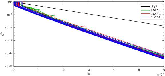
Figure 1: Convergence plots for a synthetic experiment with quadratic functions, with 15 different runs for each stochastic algorithm.

We compare SAGA, L-SVRG and ELVIRA on the same synthetic problem of minimizing over $\mathbb{R}^{d}$ the average of $M=1000$ functions $F_{m}$, with $d=100$; that is, Problem (1) with $R=0$. Every function $F_{m}$ is quadratic: $F_{m}:x\mapsto\frac{1}{2}\|A_{m}x-b_{m}\|^{2}$ for some matrix $A_{m}$ of size $d^{\prime}\times d$ and vector $b_{m}\in\mathbb{R}^{d^{\prime}}$, all made of independent random values drawn from the uniform distribution in $[0,1]$, with $d^{\prime}=5$. Since $d^{\prime}<d$, none of the $F_{m}$ is strongly convex, but their average $F$ is $\mu$-strongly convex, with $\mu\approx 0.3$. Every $F_{m}$ is $L$-smooth, with $L=\max_{m=1,\ldots,M}\|A_{m}^{*}A_{m}\|\approx 153$. We choose $b=1.4$ so that the 2 terms in the rate $c$ are equal and $\approx 0.9996$ and we set $\gamma=\frac{1}{L(1+b)^{2}}$ in the 3 algorithms. In L-SVRG and ELVIRA, $N=1$ and $p=\frac{1}{M}$. Then the Lyapunov function $\Psi^{k}$ is the same for the 3 algorithms, as well as the rate $c\approx 0.9996$. We show the upper bound $c^{k}\Psi^{0}$ in black in Figure 1. The solutions $x^{\star}$ and $h_{m}^{\star}$ were computed to machine precision by running SAGA with $10^{6}$ iterations. The value of $\Psi^{k}$ with respect to $k$ is shown in Figure 1 for the 3 algorithms, for 15 different runs of each algorithm. We can observe that the algorithms converge linearly, as proved by our convergence results, with an empirical convergence rate better than the upper bound. The 3 algorithms have rather similar convergence profiles, with convergence slightly slower for SAGA, ELVIRA performing best, with less choppy curves, and L-SVRG in between. The convergence is shown with respect to the iteration index $k$, but we should keep in mind that SAGA has 1 gradient evaluation per iteration, whereas in average L-SVRG and ELVIRA have 3. But SAGA needs to store all the vectors $h_{m}$, while L-SVRG and ELVIRA do not need such memory occupation.

References

- Albasyoni et al. (2020) A. Albasyoni, M. Safaryan, L. Condat, and P. Richtárik. Optimal gradient compression for distributed and federated learning. arXiv:2010.03246, 2020.
- Alistarh et al. (2017) D. Alistarh, D. Grubic, J. Li, R. Tomioka, and M. Vojnovic. QSGD: Communication-efficient SGD via gradient quantization and encoding. In Proc. of 31st Conf. Neural Information Processing Systems (NIPS), pages 1709–1720, 2017.
- Bach (2021) F. Bach. Learning theory from first principles. Draft of a book, version of Sept. 6, 2021, 2021.
- Basu et al. (2020) D. Basu, D. Data, C. Karakus, and S. N. Diggavi. Qsparse-Local-SGD: Distributed SGD With Quantization, Sparsification, and Local Computations. IEEE Journal on Selected Areas in Information Theory, 1(1):217–226, 2020.
- Bauschke and Combettes (2017) H. H. Bauschke and P. L. Combettes. Convex Analysis and Monotone Operator Theory in Hilbert Spaces. Springer, New York, 2nd edition, 2017.
- Combettes and Pesquet (2021) P. L. Combettes and J.-C. Pesquet. Fixed point strategies in data science. IEEE Trans. Signal Process., 69:3878–3905, 2021.
- Condat et al. (2022a) L. Condat, D. Kitahara, A. Contreras, and A. Hirabayashi. Proximal splitting algorithms for convex optimization: A tour of recent advances, with new twists. SIAM Review, 2022a. to appear.
- Condat et al. (2022b) L. Condat, G. Malinovsky, and P. Richtárik. Distributed proximal splitting algorithms with rates and acceleration. Frontiers in Signal Processing, 1, January 2022b.
- Condat et al. (2022c) L. Condat, K. Yi, and P. Richtárik. EF-BV: A unified theory of error feedback and variance reduction mechanisms for biased and unbiased compression in distributed optimization. arXiv:2205.04180, 2022c.
- Defazio et al. (2014) A. Defazio, F. Bach, and S. Lacoste-Julien. SAGA: A fast incremental gradient method with support for non-strongly convex composite objectives. In Proc. of 28th Conf. Neural Information Processing Systems (NIPS), pages 1646–1654, 2014.
- Dutta et al. (2020) A. Dutta, E. H. Bergou, A. M. Abdelmoniem, C. Y. Ho, A. N. Sahu, M. Canini, and P. Kalnis. On the discrepancy between the theoretical analysis and practical implementations of compressed communication for distributed deep learning. In Proc. of AAAI Conf. Artificial Intelligence, pages 3817–3824, 2020.
- Gazagnadou et al. (2019) N. Gazagnadou, R. Gower, and J. Salmon. Optimal mini-batch and step sizes for SAGA. In Proc. of 36th Int. Conf. Machine Learning (ICML), volume PMLR 97, pages 2142–2150, 2019.
- Gorbunov et al. (2020a) E. Gorbunov, F. Hanzely, and P. Richtárik. A unified theory of SGD: Variance reduction, sampling, quantization and coordinate descent. In Proc. of 23rd Int. Conf. Artificial Intelligence and Statistics (AISTATS), 2020a.
- Gorbunov et al. (2020b) E. Gorbunov, D. Kovalev, D. Makarenko, and P. Richtárik. Linearly converging error compensated SGD. In Proc. of 34th Conf. Neural Information Processing Systems (NeurIPS), 2020b.
- Gower et al. (2019) R. M. Gower, N. Loizou, X. Qian, A. Sailanbayev, E. Shulgin, and P. Richtárik. SGD: General analysis and improved rates. In Proc. of 36th Int. Conf. Machine Learning (ICML), volume PMLR 97, pages 5200–5209, 2019.
- Gower et al. (2020) R. M. Gower, M. Schmidt, F. Bach, and P. Richtárik. Variance-reduced methods for machine learning. Proc. of the IEEE, 108(11):1968–1983, November 2020.
- Gower et al. (2021) R. M. Gower, P. Richtárik, and F. Bach. Stochastic quasi-gradient methods: Variance reduction via Jacobian sketching. Math. Program., 188:135–192, July 2021.
- Hofmann et al. (2015) T. Hofmann, A. Lucchi, S. Lacoste-Julien, and B. McWilliams. Variance reduced stochastic gradient descent with neighbors. In Proc. of 29th Conf. Neural Information Processing Systems (NIPS), pages 1509–1519, 2015.
- Horváth et al. (2019) S. Horváth, D. Kovalev, K. Mishchenko, S. Stich, and P. Richtárik. Stochastic distributed learning with gradient quantization and variance reduction. arXiv:1904.05115, 2019.
- Johnson and Zhang (2013) R. Johnson and T. Zhang. Accelerating stochastic gradient descent using predictive variance reduction. In Proc. of 27th Conf. Neural Information Processing Systems (NIPS), pages 315–323, 2013.
- Kairouz et al. (2021) P. Kairouz et al. Advances and open problems in federated learning. Foundations and Trends in Machine Learning, 14(1–2), 2021.
- Khaled et al. (2020) A. Khaled, O. Sebbouh, N. Loizou, R. M. Gower M., and P. Richtárik. Unified analysis of stochastic gradient methods for composite convex and smooth optimization. arXiv:2006.11573, 2020.
- Konečný et al. (2016) J. Konečný, H. B. McMahan, F. X. Yu, P. Richtárik, A. T. Suresh, and D. Bacon. Federated learning: Strategies for improving communication efficiency. Paper arXiv:1610.05492, presented at the NIPS Workshop on Private Multi-Party Machine Learning, 2016.
- Kovalev et al. (2020) D. Kovalev, S. Horváth, and P. Richtárik. Don’t jump through hoops and remove those loops: SVRG and Katyusha are better without the outer loop. In Proc. of 31st Int. Conf. Algorithmic Learning Theory (ALT), volume PMLR 117, pages 451–467, 2020.
- Li et al. (2020) T. Li, A. K. Sahu, A. Talwalkar, and V. Smith. Federated learning: Challenges, methods, and future directions. IEEE Signal Processing Magazine, 3(37):50–60, 2020.
- Liu et al. (2020) X. Liu, Y. Li, J. Tang, and M. Yan. A double residual compression algorithm for efficient distributed learning. In Proc. of 23rd Int. Conf. Artificial Intelligence and Statistics (AISTATS), volume PMLR 108, pages 133–143, 2020.
- McMahan et al. (2017) H. Brendan McMahan, Eider Moore, Daniel Ramage, Seth Hampson, and Blaise Agüera y Arcas. Communication-efficient learning of deep networks from decentralized data. In Proc. of 20th Int. Conf. Artificial Intelligence and Statistics (AISTATS), 2017.
- Mishchenko et al. (2019) K. Mishchenko, E. Gorbunov, M. Takáč, and P. Richtárik. Distributed learning with compressed gradient differences. arXiv:1901.09269, 2019.
- Parikh and Boyd (2014) N. Parikh and S. Boyd. Proximal algorithms. Foundations and Trends in Optimization, 3(1):127–239, 2014.
- Philippenko and Dieuleveut (2020) C. Philippenko and A. Dieuleveut. Bidirectional compression in heterogeneous settings for distributed or federated learning with partial participation: tight convergence guarantees. arXiv:2006.14591, 2020.
- Qian et al. (2019) X. Qian, A. Sailanbayev, K. Mishchenko, and P. Richtárik. MISO is making a comeback with better proofs and rates. arXiv:1906.01474, June 2019.
- Qian et al. (2021) X. Qian, Z. Qu, and P. Richtárik. L-SVRG and L-Katyusha with arbitrary sampling. Journal of Machine Learning Research, 22(112):1–47, 2021.
- Richtárik and Takáč (2016) P. Richtárik and M. Takáč. Parallel coordinate descent methods for big data optimization. Math. Program., 156:433–484, 2016.
- Salim et al. (2022) A. Salim, L. Condat, K. Mishchenko, and P. Richtárik. Dualize, split, randomize: Fast nonsmooth optimization algorithms. Journal of Optimization Theory and Applications, 2022. to appear.
- Sattler et al. (2020) F. Sattler, S. Wiedemann, K.-R. Müller, and W. Samek. Robust and communication-efficient federated learning from non-i.i.d. data. IEEE Trans. Neural Networks and Learning Systems, 31(9):3400–3413, 2020.
- Sebbouh et al. (2019) O. Sebbouh, N. Gazagnadou, S. Jelassi, F. Bach, and R. Gower. Towards closing the gap between the theory and practice of SVRG. In Proc. of 33rd Conf. Neural Information Processing Systems (NeurIPS), 2019.
- Tang et al. (2019) H. Tang, C. Yu, X. Lian, T. Zhang, and J. Liu. Doublesqueeze: Parallel stochastic gradient descent with double-pass error-compensated compression. In Proc. of Int. Conf. Machine Learning (ICML), pages 6155–6165, 2019.
- Wangni et al. (2018) J. Wangni, J. Wang, J. Liu, and T. Zhang. Gradient sparsification for communication-efficient distributed optimization. In Proc. of 32nd Conf. Neural Information Processing Systems (NeurIPS), pages 1306–1316, 2018.
- Wen et al. (2017) W. Wen, C. Xu, F. Yan, C. Wu, Y. Wang, Y. Chen, and H. Li. TernGrad: Ternary gradients to reduce communication in distributed deep learning. In Proc. of 31st Conf. Neural Information Processing Systems (NIPS), pages 1509–1519, 2017.
- Xiao and Zhang (2014) L. Xiao and T. Zhang. A proximal stochastic gradient method with progressive variance reduction. SIAM J. Optim., 24(4):2057–2075, 2014.
- Xu et al. (2021) H. Xu, C.-Y. Ho, A. M. Abdelmoniem, A. Dutta, E. H. Bergou, K. Karatsenidis, M. Canini, and P. Kalnis. GRACE: A compressed communication framework for distributed machine learning. In Proc. of 41st IEEE Int. Conf. Distributed Computing Systems (ICDCS), 2021.
- Zhang et al. (2013) L. Zhang, M. Mahdavi, and R. Jin. Linear convergence with condition number independent access of full gradients. In Proc. of 27th Conf. Neural Information Processing Systems (NIPS), 2013.