Analysis of a semi-augmented mixed finite element method for double-diffusive natural convection in porous media ††thanks: This work was partially supported by Vicerrectoría de Investigación, through the project C00-89, Sede de Occidente, Universidad de Costa Rica; by CONICYT-Chile through the project 1190241; and by Universidad Nacional, Costa Rica, through the project 0140-20.
Abstract
In this paper we study a stationary double-diffusive natural convection problem in porous media given by a Navier-Stokes/Darcy type system, for describing the velocity and the pressure, coupled to a vector advection-diffusion equation describing the heat and substance concentration, of a viscous fluid in a porous media with physical boundary conditions. The model problem is rewritten in terms of a first-order system, without the pressure, based on the introduction of the strain tensor and a nonlinear pseudo-stress tensor in the fluid equations. After a variational approach, the resulting weak model is then augmented using appropriate redundant penalization terms for the fluid equations along with a standard primal formulation for the heat and substance concentration. Then, it is rewritten as an equivalent fixed-point problem. Well-posedness and uniqueness results for both the continuous and the discrete schemes are stated, as well as the respective convergence result under certain regularity assumptions combined with the Lax-Milgram theorem, and the Banach and Brouwer fixed-point theorems. In particular, Raviart-Thomas elements of order are used for approximating the pseudo-stress tensor, piecewise polynomials of degree and are utilized for approximating the strain tensor and the velocity, respectively, and the heat and substance concentration are approximated by means of Lagrange finite elements of order . Optimal a priori error estimates are derived and confirmed through some numerical examples that illustrate the performance of the proposed semi-augmented mixed-primal scheme.
Keywords: Double-diffusive natural convection, Oberbeck-Boussinesq model, augmented formulation, mixed-primal finite element method, fixed point theory, a priori error analysis.
Mathematical subject classifications (2020): 65N30, 65N12, 65N15, 76D05, 76R10, 76M10, 80A19.
1 Introduction
In nature and several technological applications, transport phenomena widely occur as a result of a combined heat and mass transfer that are driven by buoyancy effects due to both temperature and concentration variations (see, e.g., [15, 37, 39]). Such processes, also known as thermosolutal or double-diffusive natural convection, involving fluid circulation in a porous media, are frequently found in astrophysics, oceanology, metallurgy, electrophysics and geophysics, but also appear in several engineering applications such as filtration processes, geothermal energy exploitation, spreading on porous substrates, bio-film growth, gasification of biomass, to name a few.
From the mathematical point of view the Darcy-Oberbeck-Boussinesq model allows to adequately describe and quantify this complex flow by means of a nonlinear partial differential equations system. More precisely, the momentum and conservation of fluid mass give rise to a Navier-Stokes/Darcy type system for describing the fluid flow in the porous media which, in turn, is coupled via buoyancy forces and convective mass and heat transfer to a vector advection-diffusion equation for describing the substance concentration and the temperature, as a result of an energy and mass transfer balance (see, e.g., [37, 39]).
Many computational techniques have been developed so far in order to numerically solve and simulate this problem and related ones (see [1, 3, 10, 17, 18, 29, 30, 34, 38, 44], and the references therein). Particularly, the contributions [1, 3, 38, 29, 30, 34, 44] deal with double-diffusive convection in a cavity, whereas in [10, 17, 18] the authors consider the phenomenon in a porous media.
In [38], a finite volume method is proposed and applied to solve agro-food processes, whereas some methods based on finite elements for this problem are [1, 3]. In [1], the authors proposed stabilized finite element formulations based on the SUPG (Streamline-Upwind/Petrov-Galerkin) and PSPG (Pressure-Stabilization/Petrov-Galerkin) methods to solve the problem in unsteady state. Numerical simulations in two and three dimensions illustrate the accuracy and performance of this technique. However, the theoretical analyses of the associate continuous and the discrete variational problems as well as the convergence of the method are not carried out there, and the method only allows to carry out low-order approximations of the main unknowns. On the other hand, in [3] the problem is considered in steady state and analyzed by using the boundary control theory. The authors formulate and prove solvability results for the corresponding boundary control problem, state local uniqueness and stability of optimal solutions.
Focusing in double-diffusive viscous flow in porous media, [17] proposes a technique consisting of a projection-based stabilization method in the unsteady state. There, the convergence of the velocity, temperature and concentration in the semi-discrete case are derived. In addition, some numerical experiments are reported to confirm optimal order error estimates and to compare their results with previous ones. In [10] the authors construct a divergence-conforming primal scheme and establish the existence and uniqueness results for the continuous problem and the discrete scheme as well as convergence properties. On the other hand, in [18] the authors propose a high-order fully-mixed method based on the introduction of the velocity gradient, the temperature gradient and the concentration gradient as new unknowns into the problem. The resulting formulation has a saddle-point structure on reflexive Banach spaces for both the Navier-Stokes/Darcy and the thermal energy conservation equations. There, it is particularly shown that the discrete scheme is well-posed and an a priori error estimate for the Galerkin scheme is also derived under sufficiently small data. However, feasible finite element subspaces must be constructed over meshes with a macro-element structure in order to satisfy an inf-sup compatibility condition, which in turn significantly increased the computational cost, especially in the three-dimensional case.
According to the above discussion and in order to contribute with the design and analysis of new mixed finite schemes for simulating double-diffusive convection in porous media. The main goal of this work is precisely to propose a new semi-augmented mixed finite element method in which the strain tensor and a pseudo-stress tensor are introduced as primary unknowns of interest in the fluid equations and the pressure is eliminated from the system by its own definition. To avoid any inf-sup restriction, to guarantee greater flexibility regarding finite element spaces and lower computational cost than [18], the respective variational formulation is augmented by using appropriate redundant penalization Galerkin type-terms based on the constitutive and equilibrium equations combined with a primal formulation for the heat and substance concentration equations in standard Hilbert spaces. In this way, the aforementioned strain tensor, the nonlinear pseudostress, the velocity and a vector field whose components are the temperature of the fluid and the substance concentration are the main unknowns of the resulting coupled system. Moreover, physical boundary conditions are considered. Indeed, a no-slip condition (that is, homogeneous Dirichlet condition) for the fluid velocity, a prescribed temperature and substance concentration on a Dirichlet boundary and no heat/mass flow across an isolated surface/homogeneous Neumann condition.
Concerning the solvability analysis, we proceed similarly to [4, 19] by introducing an equivalent fixed-point setting. According to this, combining the Lax-Milgram theorem with the classical Banach and Brouwer fixed-point theorems, we establish the respective solvability of the continuous problem and the associated Galerkin scheme, under suitable regularity assumptions (see [7], for further details), a feasible choice of parameters and, in the discrete case, for any family of finite element subspaces. To handle the non-homogeneous Dirichlet condition for the temperature and concentration, we carry out a rigorous treatment of the boundary data throughout the analysis by means of appropriate extensions involving the Scott-Zhang interpolator (in the discrete case), which allows us to establish the well-posedness of our scheme, along with its convergence result and the respective a priori error bounds. Up to the best of our knowledge, because of the difficulties that can arise in the analysis, the physically relevant non-homogeneous Dirichlet condition case is usually either omitted or not considered; this is what motivates us to contribute in this direction as well.
A Strang-type lemma, enables us to derive the corresponding Céa estimate and to provide optimal a priori error bounds for the Galerkin solution. In turn, the pressure can be recovered by a post-processed of the discrete solutions, preserving the same rate of convergence. Finally, some numerical experiments are presented to illustrate the performance of the technique, including the unsteady case with unknown solution, to confirm the expected orders.
The contents of this paper is presented as follows. At the end of this section, we introduce some standard notations to be used throughout the manuscript. In Section 2, we introduce the model problem and the data. We also derive an equivalent first-order equations in terms of additional variables. Then, in Section 3, we derive the semi-augmented mixed-primal variational formulation and establish its well-posedness. The associated Galerkin scheme is introduced and analyzed in Section 4. In Section 5, we derive the corresponding Céa estimate and, finally, in Section 6 we present some numerical examples illustrating the performance of our semi-augmented mixed-primal finite element method.
1.1 Notations
Let us denote by , with , a given bounded domain with polygonal/polyhedral boundary with outward unit normal vector and let be such that , and . Standard notation will be adopted for Lebesgue spaces with norm or if , and Sobolev spaces with norm , and semi-norm . In particular, when denotes a generic scalar functional space, then we will denote its vectorial and tensor counterparts by and , respectively.
For vector fields and , we set the gradient, divergence and dyadic product operators, as
respectively. Furthermore, given the tensor fields and , we let be the divergence operator acting along the rows of , and define the transpose, the trace, the tensor inner product, and the deviatoric tensor, respectively, as
where stands for the identity tensor in . We recall that the space
equipped with the usual norm
is a Hilbert space. Finally, we employ to denote a generic null vector and use or , with or without subscripts, bars, tildes or hats, to mean generic positive constants independent of the discretization parameters, which may take different values at different places.
2 The model problem
This section introduces the mathematical model we address in the present work as well as the auxiliary unknowns that are introduced and considered in the subsequent variational formulation. Under the Oberbeck-Boussinesq approximation framework, double-diffusive natural convection phenomenon in a porous media is described in terms of a Navier-Stokes-Brinkman model coupled to a system of diffusion-advection equations. In the stationary state, the problem consists of finding the velocity , the pressure , and the vector when and when , where and are the temperature and the concentration fields, respectively, of a fluid in a confined porous enclosure , satisfying the set of equations:
| (2.1) |
where stands for the symmetric part of the velocity gradient, i.e., . The data are the gravitational force , the positive constant corresponding to the reciprocal of the Darcy number, the (thermal and solute) expansion coefficients vector , and the diagonal matrix of (thermal and mass) diffusion constants , with when , which is assumed to be a uniformly positive definite tensor, which means that there exists a positive constant such that
| (2.2) |
In turn, the kinematic viscosity is assumed to be a bounded and Lipschitz continuous function that might depend on both the temperature and the mass concentration. That is, we assume the existence of positive constants and that satisfy
| (2.3) |
The system (2.1) is finally completed with a non-slip condition on the whole boundary for the velocity and physical boundary conditions for both the temperature and the concentration fields, that is
| (2.4) |
where is a known trace function on
Next, proceeding similarly to [13], we introduce the strain tensor as an auxiliary variable and then define
| (2.5) |
as an additional tensorial unknown, where is a constant to be suitably defined next (see equation (2.7) below). Thus, noting that the incompressibility condition of the fluid implies that , we get from the first relation of (2.1) the equilibrium equation
and taking deviatoric part in (2.5), we find that the constitutive relation defined by (2.5) can be written as
where since Thus, the pressure is eliminated from the system, however taking trace in (2.5), we find that it can be easily recovered according to the formula
| (2.6) |
Now, since (which as usual is clearly required for uniqueness of an eventual pressure solution to (2.1)), the equation (2.6) suggests to define
| (2.7) |
so as to get the equivalence
| (2.8) |
According to the above discusion, the system (2.1) and (2.4) equivalently reads: Find , and such that
| (2.9) |
where is the skew-symmetric part of the velocity gradient. We emphasize that the introduction of the variables and as new unknowns in the system allows us to equivalently rewrite the Navier-Stokes-Brinkman model (first row of (2.1)) in terms of a first-order set of equations. Also, observe that according to (2.6)-(2.8), the zero mean value restriction of the pressure on the domain is imposed via the respective restriction on in the last equation of (2.9). Note further that the incompressibility condition of the fluid is implicitly present via the equilibrium relation defined by according to the second equation in the first row of (2.9).
3 The continuous formulation
In this section we introduce and analyze the weak formulation proposed for the system described by (2.9). In Section 3.1 we firstly deduce an augmented mixed variational formulation of (2.9) and then we rewrite it as a fixed-point problem in Section 3.2, whose analysis is addressed through Sections 3.3 and 3.4.
3.1 The semi-augmented mixed-primal variational formulation
To begin with, the fact that the trace of the tensor solution of system (2.9) has zero mean value in (see last equation of (2.9)) suggests to introduce the space
In addition, by their own definitions, we introduce the following space for the strain tensor , as
In turn, because of the boundary conditions for the temperature and concentrations (see second and third equations of last row in (2.9)) we consider the closed subspace
for which, from the generalized Poincaré inequality, we know that there exists , depending only on and , such that
| (3.1) |
Now, testing the first equation from first row in (2.9) with , we obtain
| (3.2) |
At this point, we readily note that in order to bound the third term on the left hand side of (3.2), and thanks to the continuous injection (see e.g. [2] or [41]), we requiere the unknown to live in . Indeed, by applying Cauchy-Schwarz and Hölder inequalities, we deduce that there exists a positive constant , such that
| (3.3) |
Next, multiplying the first equation from second row in (2.9) by a test function , integrating by parts, using the Dirichlet condition for , and the identity (since is trace-free), we get
Likewise, the equilibrium relation associated to (second equation from first row in (2.9)) is written as
whereas, the symmetry of the pseudo-stress tensor is imposed in an ultra-weak sense (see e.g [8]) through the identity
As for the equation associated to the temperature and concentration (second equation from second row in (2.9)), we simply multiply it by a test function and, after integrating by parts, and employing the Neumann boundary contidions on , we find
In this way, a preliminary weak formulation for the coupled problem (2.9) takes the form: Find , with , such that
| (3.4) |
In order to analyze the variational formulation (3.4), and similarly as in [13, Section 2] (see also [4, 8, 21]), we additionally augment (3.4) by incorporating the following residual Galerkin type-terms coming from the constitutive and equilibrium equations for the fluid,
| (3.5) |
where is a vector of positive parameters to be specified later in Section 3.3.
Hence, letting
where is endowed with the natural norm
and adding up (3.4) with (3.5), we arrive at the following semi-augmented mixed-primal formulation for the double-diffusive natural convection problem in porous media: Find , with , such that
| (3.6a) | |||||
| (3.6b) | |||||
where, given and , , and are the bilinear forms defined, respectively, as
| (3.7) |
and
| (3.8) |
for all and
| (3.9) |
In turn, and are linear functionals defined as
| (3.10) |
and
| (3.11) |
3.2 The fixed point approach
In this Section we describe a fixed point strategy that allow us to solve the coupled problem given by (3.6). We start by denoting , and defining the operator by
where is the unique solution of the augmented mixed formulation given by (3.6a), with instead , that is:
| (3.12) |
where the bilinear forms , and the functional are defined exactly as in (3.7), (3.8), and (3.10), respectively. In addition, we also introduce the operator defined as
where is the unique solution of the problem (3.6b), with instead , that is:
| (3.13) |
where the bilinear form , and the functional are defined by (3.9) and (3.11), respectively.
3.3 Well-posedness of the uncoupled problems
We begin by recalling the following lemmas which are useful to prove the ellipticity of the bilinear form .
Lemma 3.1
There exists such that
with and .
Proof. See [9, Proposition 3.1].
Lemma 3.2
There holds
Proof. See [36, Theorem 10.1].
We now provide sufficient conditions under which the uncoupled problems (3.12) and (3.13) are indeed uniquely solvable.
Lemma 3.3
Assume that , , with , , . Then, there exists such that for each , problem (3.12) has a unique solution , for each with . Moreover, there exists , independent of , such that
| (3.16) |
Proof. We begin by deriving the continuity of the bilinear forms and (sf. (3.7) and (3.8), respectively). Indeed, applying Cauchy-Schwarz’s inequality, the assumptions (2.3), and the fact that and , we deduce that there exists a positive constant , depending on , such that
| (3.17) |
where . In turn, by applying Hölder’s inequality and the continuous injection , with constant , we obtain that
| (3.18) |
Then, it follows from (3.17) and (3.18), that there exists a positive constant denote by , that depends on and , such that
| (3.19) |
We now address the proof of the ellipticity for the bilinear form . To this end, we first derive this property for the bilinear form . In fact, from (3.7), by applying (2.3) and the Cauchy-Schwarz inequality, together with Lemma 3.2, it followss that
Next, employing the Young inequality and gathering similar terms, we obtain
and then, choosing , , , , and in the ranges specified of the statement of the present Lemma, we deduce that there exists a positive constant , independent of , such that
| (3.20) |
Next, by combining (3.18) and (3.20), we find that
from which, we deduce that
| (3.21) |
provided that , with
| (3.22) |
which confirms the ellipticity of . On the other hand, by applying the Cauchy-Schwarz inequality, we deduce that (cf. (3.10)) with
| (3.23) |
Consequently, a straightforward application of the Lax-Milgram lemma implies that there exists a unique solution of (3.12). Finally, from (3.21) and (3.23), and performing simple algebraic manipulations, we derive (3.16), with , independent of .
Remark 3.1
At this point, we remark that for computational purposes, the constant defined in Lemma 3.3, can be maximized by choosing the parameters , , , , and at the middle points of their feasible ranges. Thus, adequate choices for these parameters are , and , which establish that
| (3.24) |
Remark 3.2
In order to establish the solvability of the problem (3.13), associated to the operator , we first point out that can be continuously extended in the trace sense to . Indeed, the set
is a closed and convex since the usual trace operator is linear and continuous. Then, from The Best Approximation Theorem [24, Theorem 7] there exists a unique , where denotes the extension of , such that with
| (3.25) |
In this way, the suitable extension of is not but the corresponding one of to .
Lemma 3.4
For each , problem (3.13) has a unique solution , with . Moreover, there exists a constant independent of , such that
| (3.26) |
Proof. We begin by nothing, according to the aforementioned in Remark 3.2, that given there exists such that
| (3.27) |
Then, we consider the auxiliary linear problem: Find such that
| (3.28) |
where and are defined in (3.9) and (3.11), respectively. In addition, from (3.9) and the Cauchy-Schwarz’s inequality, we deduce that
| (3.29) |
which, in particular, confirms the boundedness of . Then, from (3.9), using (2.2) and the Poncairé inequality (3.1), we get
| (3.30) |
which proves that is -elliptic with constant
| (3.31) |
Next, applying the Cauchy-Schwarz’s inequality, the boundedness of the continuous injection , with constant , (3.29), and the second identity in (3.27), we easily deduce that
| (3.32) |
which establishes the boundedness of the right-hand side of (3.28). Consequently, a direct application of the Lax-Milgram lemma implies that there exists a unique that satisfies (3.28) with
On the other hand, we now set , which satisfies that . In addition, it is easy to check that is a solution of problem (3.13), where the uniqueness comes from (3.30). Finally, verifies the estimate (3.26), with constant .
We end this section by introducing a further regularity hypotheses on the problem definig , which will be employed to derive a Lipschitz-continuity property for the operator . More precisely, we assume that for each with , given, there holds , for some (when ) or (when ), with
| (3.33) |
where is a positive constant independent of but depending on the upper bound of its norm. The reason of the estipulated ranges for will be clarified in the forthcomming analysis (specifically in the proofs of Lemmas 3.6 and 3.8 below). Also, we pay attention to the fact the while the estimate (3.33) will be employed only to bound , we have stated it including the terms and as well, since due to the first and fourth equations of (2.9), the regularities of and will most likely be connected.
3.4 Solvability analysis of the fixed point equation
We begin by emphasizing that the well-posedness of the uncoupled problems (3.12) and (3.13) confirms that the operators , , and (cf. (3.14)) are well defined, and hence now we can address the solvability analysis of the fixed point problem presented in (3.15). To this end, we will verify below the hypotheses of the Banach fixed-point theorem.
Lemma 3.5
Proof. It follows similar as in [20, Lemma 3.5]
Lemma 3.6
Proof. Given as stated, we let and , which according to the definition of operator (cf. (3.12)), means that:
Then, subtracting both identities, replacing , and using the bilinearity of for any and , it follows from (3.12) that:
| (3.36) |
Moreover, applying the ellipticity of (cf. (3.21)), and then employing (3.36) with , we find that
| (3.37) | |||||
Then, for the first and third terms on the right-hand side of (3.37), we employ the Cauchy-Schwarz and Hölder inequalities, together with the continuous injection , similar as in (3.23) and (3.18), in order to obtain that
| (3.38) |
and
| (3.39) |
On the other hand, for the second term in the right-hand side of (3.37), we apply the Lipschitz continuity property for given in (2.3), the Cauchy-Schwarz and Hölder inequalities, and the definition of (cf. (3.7)), to obtain that
| (3.40) |
with such that We now proceed as in [7, Lemma 3.9]. In fact, given the further -regularity assumed in (3.33), we reall that the Sobolev embedding theorem (see e.g [2, Theorem 4.12]) establishes the continuous injection with boundedness constant , where
and , and therefore, there holds
| (3.41) |
In this way, denoting
from the inequalities (3.37), (3.38), (3.39), (3.40), and recalling that and , yields (3.35) and concludes the proof.
Lemma 3.7
Proof. Given , we let be the corresponding solutions of (3.13), that is and . Then, since , we realize that belongs to . In this way, applying the ellipticity of (cf. (3.30)), using (3.13) and (3.11), adding and subtracting , and employing the Hölder inequality, the continuous injection , and the definition of (cf. Lemma 3.5), we readily deduce that
which give (3.42) with .
Lemma 3.8
Proof. Given and , we first observe, according to the definition of (cf. (3.14)), and the Lipschitz-continuity of (cf. (3.42)), that
from which, employing the Lipschitz-continuity of (cf. (3.6)), yields
| (3.45) |
Then, applying the bound (3.16) to estimate the term , employing the continuous injection of into with boundedness constant , using the estimate (3.33) to estimate the term , noting that , and performing some algebraic manipulations, we get from (3.45) that
In this way, (3.44) follows from the foregoing inequality by defining
| (3.46) |
in order to complete the proof.
Theorem 3.9
4 Galerkin scheme
In this section we introduce and analyze the Galerkin scheme of the semi-augmented mixed-primal problem (3.6). To this end, we now let be a regular triangulation of by triangles (in ) or tetrahedra ( in ) of diameter , and define the meshsize . In addition, given an integer , for each we let be the space of polynomial functions on of degree , and define the corresponding local Raviart-Thomas space of order as
where, according to the notations described in Section 1.1, , and is the generic vector in . Then, we consider piecewise polynomials of degree for approximating entries of the strain rate , the global Raviart-Thomas space of order to approximate rows of the pseudostress , and the Lagrange space given by the continuous piecewise polynomial vectors of degree for the velocity , respectively, that is
| (4.1) | |||||
| (4.2) | |||||
| (4.3) |
For the unknown containing the tempeture and the concentration into its coordinates, we let denote the Lagrange space of degree with respect to (similar to ), and set
| (4.4) |
to be the analogous space with homogeneous Dirichlet boundary conditions. We define
| (4.5) |
to be the approximate Dirichlet boundary data, where denotes the Scott-Zhang interpolant operator of degree , which satisfies the following stability and approximation properties, respectively, (see [25, Lemma 1.130]).
Lemma 4.1
Let and satisfy and if , and otherwise. Then, there exists a positive constant , independent of , such that the following properties hold:
-
For all ,
(4.6) -
Provided , for all ,
(4.7) where denotes the set of elements in , sharing at least one vertex with .
Hence, belongs to the discrete trace space on given by
where stands for the set of edges/faces on .
In this way, defining and denoting , the underlying Galerkin scheme given by the discrete counterpart of (3.6), reads: Find , with , such that
| (4.8a) | |||||
| (4.8b) | |||||
Throughout the rest of this section we adopt the discrete analogue of the fixed point strategy introduced in Section 3.2. Indeed, denoting , we define the operator by
where is the unique solution of the discrete problem (4.8a) with instead pf , that is
| (4.9) |
where the bilinear forms , and the functional are those corresponding to (3.7), (3.8), and (3.10), respectively, with and .
In addition, we introduce the operator defined as
where is the unique solution of the discrete problem (4.8b) with instead pf , that is
| (4.10) |
where the bilinear form , and the functional are defined as in (3.9) and (3.11), respectively, with and .
Therefore, by introducing the operator as
we realize that solving (4.8) is equivalent to seeking a fixed point of , that is: Find such that
| (4.11) |
Certainly, all the above makes sense if we guarantee that the discrete problems (4.9) and (4.10) are well-posed. This is precisely the purpose of the next section.
4.1 Well-posedness of the uncoupled problems
In this section, we establish the well-posedness of both (4.9) and (4.10), thus confirming that the operators , , and hence , are well-defined. We begin with the corresponding result for , which actually follows almost verbatim to that of its continuous counterpart (see Lemma 3.3), and the proof can be omitted.
Lemma 4.2
We now provide the discrete version of Lemma 3.4.
Lemma 4.3
For each , problem (4.10) has a unique solution , with . Moreover, there exists a constant independent of , such that
| (4.12) |
Proof. Let which satisfies . Then, similar to Lemma 3.4, we consider the auxiliary discrete problem: Find such that
| (4.13) |
where
Next, the boundedness and the ellipticity of are obtained exactly as in the proof of Lemma 3.4 with the same ellipticity constant given by (3.31). On the other hand, reasoning as in the proof of Lemma 3.4, and applying the stability property of (cf. (4.6)) and the equinormic property of (cf. (3.27)), we easily deduce that
, which says that and
Therefore, a direct application of the Lax-Milgram lemma implies that there exists a unique that satisfies (4.13) with
Then, , which in fact satisfies that , is the unique solution of (4.10). In addition, the estimate (4.12) holds with .
4.2 Solvability analysis of the fixed point equation
In this section we establish the solvability of the fixed point problem (4.11) by applying the Brouwer fixed-point theorem [16, Theorem 9.9-2]. To this end, we begin with the discrete version of lemma 3.5.
Lemma 4.4
In order to provide the discrete analogue of Lemma 3.6, we notice in advance that, instead of the regularity assumptions employed in the continuous case, which are not applicable in the present case, we simple utilize an -- argument.
Lemma 4.5
Let with given by (3.22). Then, there exists a constant , independent of , such that for all , with , there holds
| (4.15) |
Proof. It proceeds exactly as in the proof of Lemma 3.6, except for the derivation of the discrete analogue of (3.40), where, instead of choosing the values of determined by the regularity parameter , it suffices to take , thus obtaining
for all , with and . Thus, since the elements of are piecewise polynomials, we can guarantee that for each . The proof concludes with .
The discrete version of Lemma 3.7 is given as follows.
Lemma 4.6
Let as in Lemma 3.7. Then, for all there holds
| (4.16) |
Proof. It corresponds to an adaptation of the proof of Lemma 3.7 to the discrete context.
Now, combining Lemmas 4.5 and 4.6, and employing the continuous injection of into , we can prove the discrete version of Lemma 3.8.
Lemma 4.7
Consequently, since the foregoing lemma confirms the continuity of , by a straightforward application of Brouwer fixed point theorem (cf. [16, Theorem 9.9-2]) on the convex and compact set , we can provide the main result of this section.
5 A priori error analysis
We now aim to derive the a priori error estimates for the Galerkin scheme given by (4.8). To this end, given , with and , with solutions of (3.6) and (4.8), respectively, we first observe that the above problems can be rewritten as two pairs of corresponding continuous and discrete formulations, namely
| (5.1a) | |||||
| (5.1b) | |||||
and
| (5.2a) | |||||
| (5.2b) | |||||
Our goal is to obtain an upper bound for the error . For this purpose, we first recall from [43, Theorem 11.1] an abstract result that corresponds to the standar Strang Lemma for elliptic variational problems, which will be straightforwardly applied to the pair (5.1a)-(5.1b).
Lemma 5.1
Let be a Hilbert space, , and be a bounded and -elliptic bilinear form. In addition, let be a sequence of finite dimensional subspaces of , and for each consider a bounded bilinear form and a functional . Assume that the family is uniformly elliptic, that is, there exists a constant , independent of such that
In turn, let and such that
Then for each there holds
where .
In what follows, as usual, we denote
We now derive the a preliminary estimate for the error .
Lemma 5.2
There exists a constant independent of , such that
| (5.3) | |||||
Proof. From Lemma 3.3 we have that the bilinear forms and are both bounded and uniformly elliptic, with ellipticity constant (cf. (3.21)). In turn, and are linear bounded functionals in and respectively. Then, a straightforward application of Lemma 5.1 to the context given by (5.1a)-(5.1b), gives
| (5.4) |
where . It is important to recall here, from (3.19), that depends only on , , , , , and , where . Furthermore, we now proceed to estimate each term appearing at the right-hand side of (5.4). In order to do that, we first apply the same arguments employed to obtain (3.38), to find that
| (5.5) |
Next, in order to estimate the last supremum in (5.4), we add and subtract , we note that
where, applying the same approach used in (3.40) and (3.39), together with (3.41) and the continuous embedding with constant , and the boundedness of the bilinear forms and , it follows that
| (5.6) |
In this way, by replacing (5.5) and (5.6) back into (5.4), we obtain (5.3) with is a positive constant depending on , , , , , , , , , , and .
The following result present a estimate for the error .
Lemma 5.3
Proof. We proceed similarly as in the proof of [6, Lemma 5.3]. Indeed, by applying the triangle inequality we have that
| (5.9) |
where . Moreover, nothing that , we can employ [45, eq. (2.17)] and (4.5), to obtain that . Now, utilizing the ellipticity of bilinear the form on (see the proof of Lemma 4.3) with constant , along with the fact that and (see (5.2)), we deduce that
| (5.10) | |||||
Next, we apply the estimate (3.4) to bound the first term on the right-hand side of (5.10), whereas for second term we use the boundedness of (cf. (3.29)), and (5.7). Then, it follows that
| (5.11) | |||||
Then, by replacing (5.11) back into (5.9), we conclude (5.8) with .
We now proceed to combine Lemmas 5.2 and 5.3 to derive the Céa estimate for the total error
In fact, by replacing the estimate for given by (5.8) into the right-hand side of (5.3), and using the fact that (cf. (3.48)) and (cf. (3.33)) along with , we find that
where and . In this way, assuming that the data and satisfy that
| (5.12) |
we can conclude that
| (5.13) |
Consequently, we now can establish the following main result.
Theorem 5.4
In order to provided the result concerning to the theoretical rate of convergence of (4.8), we recall from [27], the approximation properties of the specific finite element subspaces introduced in Section 4.
() There exists , independent of , such that for each , and for each , there holds
() There exists , independent of , such that for each , and for each , with , there holds
() There exists , independent of , such that for each , and for each , there holds
Finally, thanks to the approximation property of given in Lemma 4.1, there exists , independent of , such that for each , and for each , there holds
Therefore, from the Céa estimate (5.14), employing the aforementioned approximation properties, we can establish the following result.
6 Numerical results
In this section we present three numerical experiments illustrating the performance of our semi-augmented mixed-primal finite element scheme (4.8), and confirming the rates of convergence provided by Theorem 5.5. More precisely, we take the stabilization parameters , and as in (3.24), which satisfies the assumption of Lemma 4.2. In addition, the zero integral mean condition for tensors in the space (4.2) is imposed via a real Lagrange multiplier. In turn, the nonlinear algebraic systems obtained are solved by the fixed-point method with a tolerance of , along with the Newton method for approximate the solution of (4.8a) in each fixed-point’s iteration. We take as initial guess the solution of a similar linear problem (in particular, satisfying the boundary conditions for and ). The numerical results presented below were obtained using a C++ code, where the corresponding linear systems arising from (4.8a) are solved using the BiCGSTAB method, whereas for (4.8b) we employ the Conjugate Gradient method as the main solver. Finally, in all experiments we let be the gravitational force, and utilizing structure triangulations of the corresponding domain in 2D. Furthermore, for the first two examples we consider polynomial degrees , whereas we only use in the last example.
We now introduce some additional notation. The individual errors are denoted by:
where, according to (2.6) and (2.7), can be computed as:
On the other hand as is usual, we let be the experimental rate of convergence given by
where and denote errors computed on two consecutive meshes of sizes and , respectively. In addition, stands for the total number of degrees of freedom (unknowns) of (4.8), that is,
Example 1. We first consider the square , and set , , , (here and ), , the thermal conductivity , and adequately manufacture the data so that the exact solution is given by the smooth functions
and
for all . In Table 1, we summarize the convergence history of the finite element scheme (4.8) as applied to Example 1. We notice there that the rate of convergence predicted by Theorem 5.5 is attained by all the unknowns.
| 0.0404 | 17575 | 7.98e-01 | 2.68e+00 | 1.37e+00 | 4.13e-02 | 1.09e-01 | ||||||
| 0.0314 | 28895 | 6.05e-01 | 1.10 | 2.09e+00 | 1.00 | 1.05e+00 | 1.05 | 3.20e-02 | 1.02 | 8.53e-02 | 0.98 | |
| 0.0257 | 43015 | 4.87e-01 | 1.09 | 1.71e+00 | 1.00 | 8.51e-01 | 1.05 | 2.61e-02 | 1.01 | 6.99e-02 | 0.99 | |
| 0.0218 | 59935 | 4.07e-01 | 1.07 | 1.45e+00 | 1.00 | 7.16e-01 | 1.04 | 2.20e-02 | 1.01 | 5.92e-02 | 1.00 | |
| 0 | 0.0189 | 79655 | 3.50e-01 | 1.06 | 1.25e+00 | 1.00 | 6.18e-01 | 1.03 | 1.91e-02 | 1.01 | 5.13e-02 | 1.00 |
| 0.0129 | 170725 | 2.35e-01 | 1.04 | 8.54e-01 | 1.00 | 4.18e-01 | 1.02 | 1.30e-02 | 1.00 | 3.49e-02 | 1.00 | |
| 0.0094 | 316805 | 1.71e-01 | 1.02 | 6.27e-01 | 1.00 | 3.05e-01 | 1.01 | 9.52e-03 | 1.00 | 2.56e-02 | 1.00 | |
| 0.0071 | 562405 | 1.28e-01 | 1.01 | 4.70e-01 | 1.00 | 2.29e-01 | 1.01 | 7.14e-03 | 1.00 | 1.92e-02 | 1.00 | |
| 0.0057 | 878005 | 1.02e-01 | 1.00 | 3.76e-01 | 1.00 | 1.83e-01 | 1.01 | 5.71e-03 | 1.00 | 1.54e-02 | 1.00 | |
| 0.0404 | 59645 | 5.37e-02 | 1.77e-01 | 8.81e-02 | 1.45e-04 | 7.38e-03 | ||||||
| 0.0314 | 98285 | 3.20e-02 | 2.07 | 1.07e-01 | 1.99 | 5.28e-02 | 2.04 | 8.48e-05 | 2.12 | 4.53e-03 | 1.94 | |
| 1 | 0.0257 | 146525 | 2.12e-02 | 2.05 | 7.18e-02 | 2.00 | 3.51e-02 | 2.03 | 5.61e-05 | 2.06 | 3.05e-03 | 1.96 |
| 0.0218 | 204365 | 1.51e-02 | 2.04 | 5.14e-02 | 2.00 | 2.51e-02 | 2.02 | 4.00e-05 | 2.03 | 2.20e-03 | 1.97 | |
| 0.0189 | 271805 | 1.13e-02 | 2.03 | 3.86e-02 | 2.00 | 1.88e-02 | 2.02 | 3.00e-05 | 2.01 | 1.66e-03 | 1.98 | |
| 0.0129 | 583445 | 5.19e-03 | 2.02 | 1.80e-02 | 2.00 | 8.70e-03 | 2.01 | 1.39e-05 | 2.01 | 7.75e-04 | 1.98 | |
| 0.0404 | 126215 | 2.70e-03 | 8.82e-03 | 3.76e-03 | 3.25e-07 | 3.45e-04 | ||||||
| 0.0314 | 208175 | 1.26e-03 | 3.04 | 4.15e-03 | 2.99 | 1.76e-03 | 3.03 | 1.47e-07 | 3.17 | 1.63e-04 | 2.99 | |
| 2 | 0.0257 | 310535 | 6.87e-04 | 3.03 | 2.28e-03 | 3.00 | 9.58e-04 | 3.02 | 7.96e-08 | 3.05 | 8.92e-05 | 2.99 |
| 0.0218 | 433295 | 4.15e-04 | 3.01 | 1.36e-03 | 3.08 | 5.79e-04 | 3.02 | 4.79e-08 | 3.04 | 5.40e-05 | 3.01 | |
| 0.0189 | 576455 | 2.70e-04 | 3.00 | 8.83e-04 | 3.03 | 3.76e-04 | 3.01 | 3.10e-08 | 3.03 | 3.51e-05 | 3.00 |
Example 2. Next, we adapt [11, Example 3], and consider the -shaped domain , and set , , , (once again and ), , , and adequately manufacture the data so that the exact solution is given by the smooth functions
for all , where is such that holds (). In addition, we remark here that the partial derivatives of , and hence, in particular , are singular at the origin. Indeed, according to the power , there holds and for each . In fact, in Table 2 we present the corresponding convergence history of Example 2, where, as predicted in advance, we note that the orders and are attained by and , respectively. Once again, the rate of convergence predicted by Theorem 5.5 is attained by all the unknowns, except for the variable that preserves . The foregoing phenomenon could be a special feature of this example. Furthermore, the results in Example 2 suggest that our approach should certainly be strengthened with the further incorporation of an adaptive strategy based on a suitable a-posteriori error estimates. This issue will also be addressed in a forthcoming paper.
| 0.0707 | 17285 | 5.60e-02 | 2.77e-01 | 7.07e-02 | 1.02e-01 | 4.85e-02 | ||||||
| 0.0566 | 26855 | 4.48e-02 | 1.00 | 2.23e-01 | 0.97 | 5.66e-02 | 1.00 | 8.15e-02 | 1.00 | 3.88e-02 | 1.00 | |
| 0.0471 | 38525 | 3.73e-02 | 1.00 | 1.87e-01 | 0.97 | 4.72e-02 | 1.00 | 6.80e-02 | 1.00 | 3.23e-02 | 1.00 | |
| 0 | 0.0404 | 52295 | 3.20e-02 | 1.00 | 1.61e-01 | 0.96 | 4.04e-02 | 1.00 | 5.83e-02 | 1.00 | 2.77e-02 | 1.00 |
| 0.0354 | 68165 | 2.80e-02 | 1.00 | 1.42e-01 | 0.96 | 3.54e-02 | 1.00 | 5.10e-02 | 1.00 | 2.42e-02 | 1.00 | |
| 0.0236 | 152645 | 1.87e-02 | 1.00 | 9.63e-02 | 0.95 | 2.36e-02 | 1.00 | 3.40e-02 | 1.00 | 1.61e-02 | 1.00 | |
| 0.0166 | 305495 | 1.32e-02 | 1.00 | 6.94e-02 | 0.94 | 1.66e-02 | 1.00 | 2.40e-02 | 1.00 | 1.14e-02 | 1.00 | |
| 0.0135 | 465575 | 1.07e-02 | 1.00 | 5.69e-02 | 0.93 | 1.35e-02 | 1.00 | 1.94e-02 | 1.00 | 9.22e-03 | 1.00 | |
| 0.0707 | 58565 | 2.34e-04 | 2.67e-02 | 1.35e-04 | 1.45e-03 | 7.06e-04 | ||||||
| 0.0566 | 91205 | 1.56e-04 | 1.82 | 2.30e-02 | 0.68 | 9.20e-05 | 1.71 | 9.30e-04 | 2.00 | 4.62e-04 | 1.90 | |
| 1 | 0.0471 | 131045 | 1.12e-04 | 1.81 | 2.03e-02 | 0.67 | 6.75e-05 | 1.69 | 6.46e-04 | 2.00 | 3.27e-04 | 1.89 |
| 0.0404 | 178085 | 8.47e-05 | 1.81 | 1.83e-02 | 0.67 | 5.21e-05 | 1.69 | 4.75e-04 | 2.00 | 2.44e-04 | 1.89 | |
| 0.0354 | 232325 | 6.66e-05 | 1.80 | 1.68e-02 | 0.67 | 4.16e-05 | 1.68 | 3.63e-04 | 2.00 | 1.90e-04 | 1.88 | |
| 0.0236 | 521285 | 3.23e-05 | 1.79 | 1.28e-02 | 0.67 | 2.11e-05 | 1.68 | 1.62e-04 | 2.00 | 8.93e-05 | 1.86 | |
| 0.0707 | 123845 | 3.00e-05 | 1.52e-02 | 3.29e-05 | 1.64e-05 | 8.29e-05 | ||||||
| 0.0566 | 193055 | 2.07e-05 | 1.67 | 1.31e-02 | 0.67 | 2.27e-05 | 1.67 | 8.39e-06 | 3.01 | 5.70e-05 | 1.68 | |
| 2 | 0.0471 | 277565 | 1.52e-05 | 1.67 | 1.16e-02 | 0.67 | 1.67e-05 | 1.67 | 4.85e-06 | 3.01 | 4.20e-05 | 1.67 |
| 0.0404 | 377375 | 1.18e-05 | 1.67 | 1.05e-02 | 0.67 | 1.29e-05 | 1.67 | 3.05e-06 | 3.00 | 3.25e-05 | 1.67 | |
| 0.0354 | 492485 | 9.44e-06 | 1.67 | 9.60e-03 | 0.67 | 1.04e-05 | 1.67 | 2.04e-06 | 3.00 | 2.60e-05 | 1.67 |
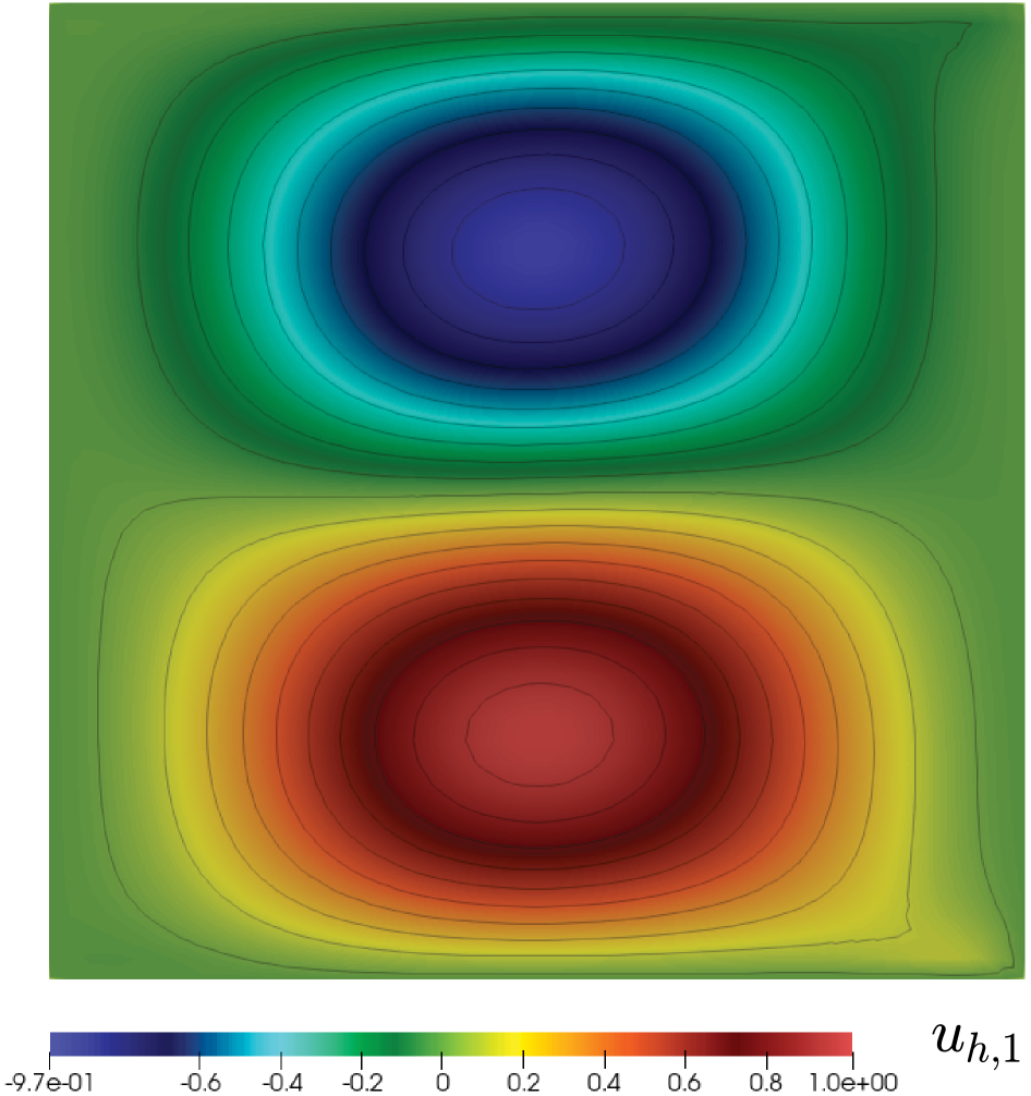
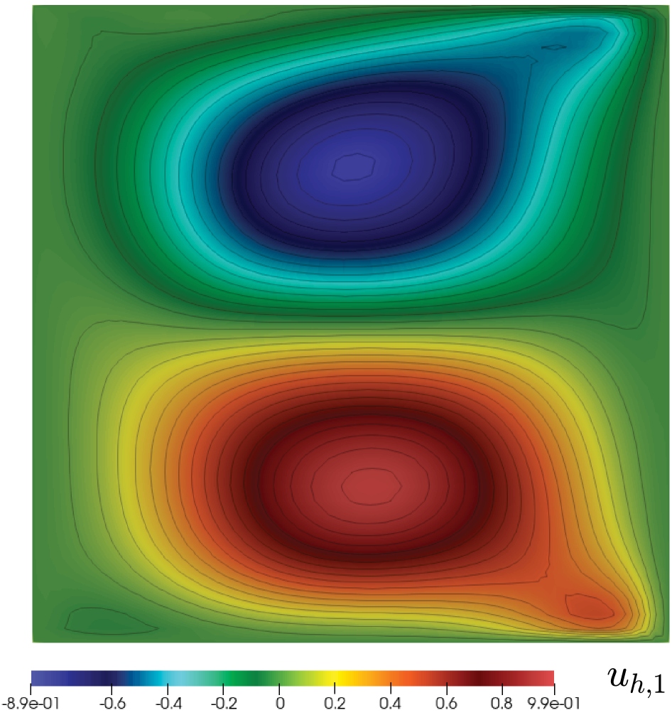
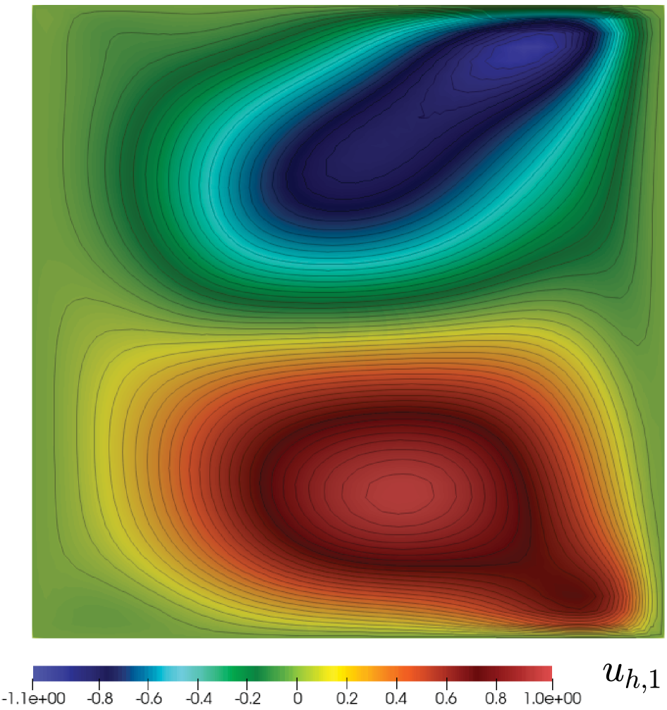
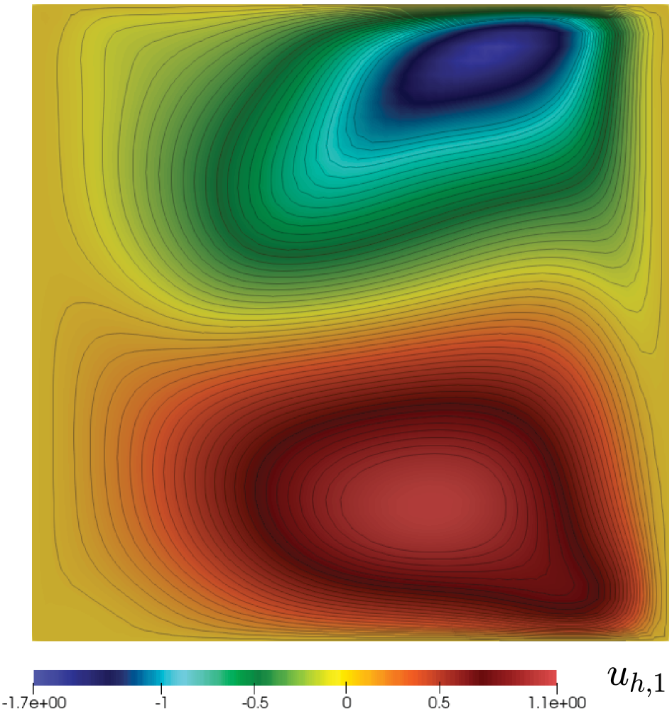
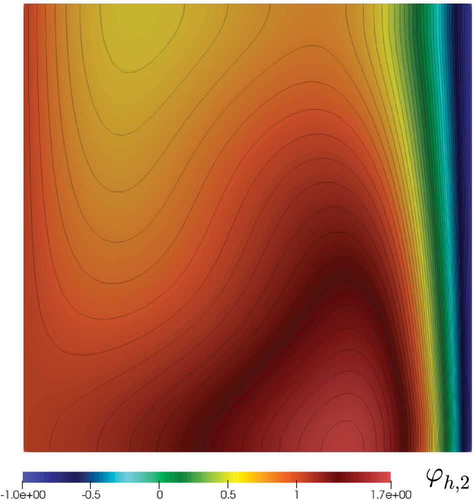
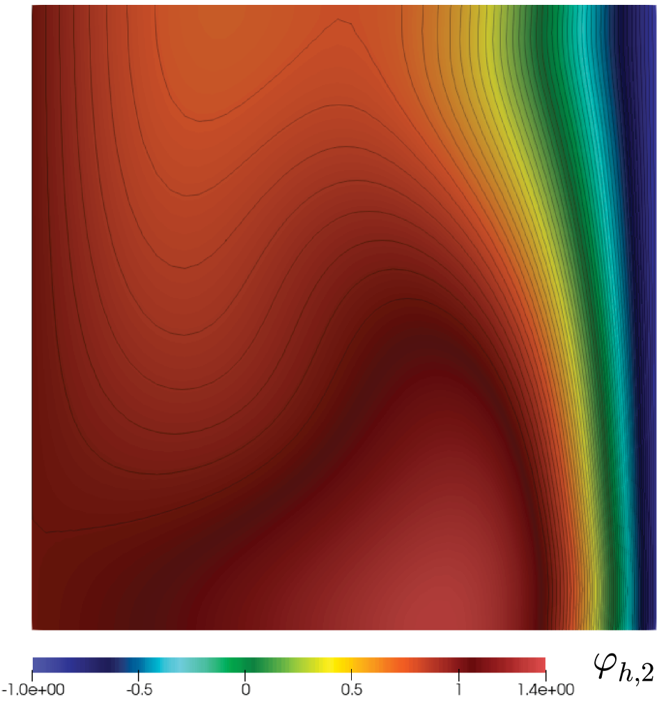
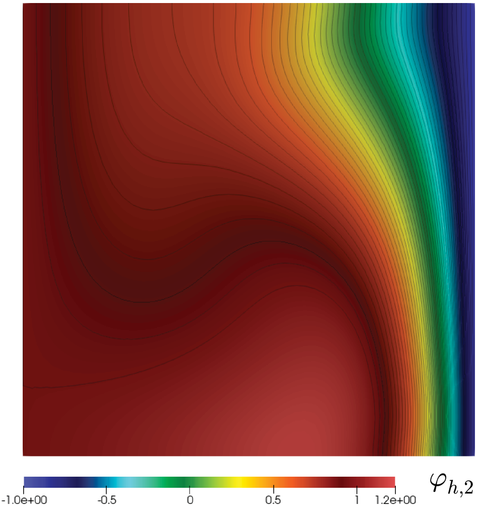
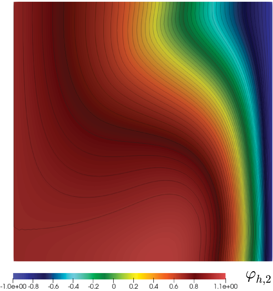
Example 3. Finally, we aim to illustrate the accuracy of our method by considering a case in which the exact solution is unknown in the a time-dependent approach. More precisely, we add and to the left-hand side of first and last equations of (2.1), respectively, which, together with the boundary conditions (2.4), we consider initial conditions
We remark here that, in similar way of [33], the analysis presented along of this paper can be extended to this time-dependent problem by employing backward Euler time stepping in order to obtain a fully-discrete method. On the other hand, for this example we consider once again the unit square , and set , , , , , . The boundary condition is defined as
for all , whereas the initial conditions are given by
In addition, for the time stepping technique we use .
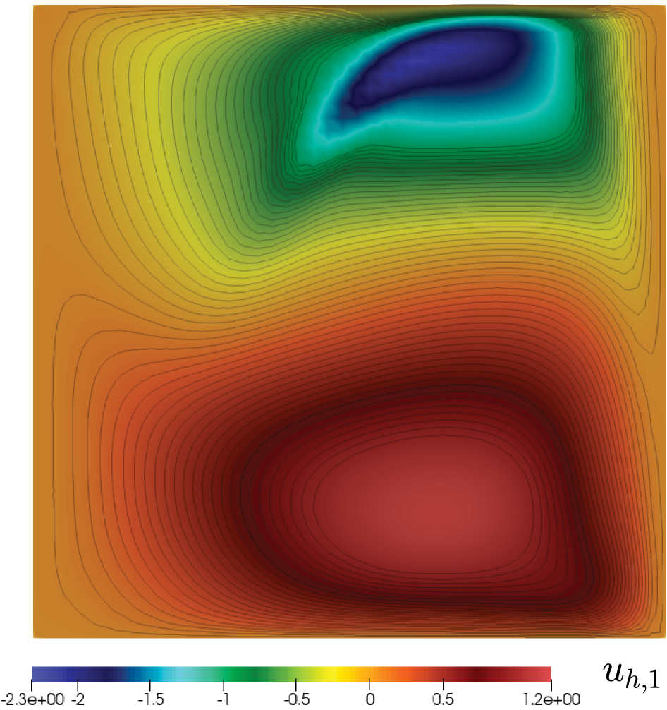
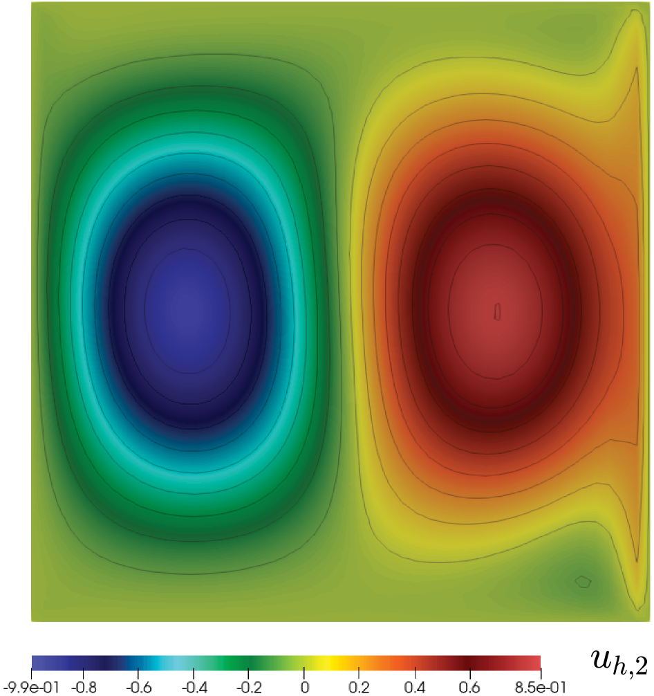
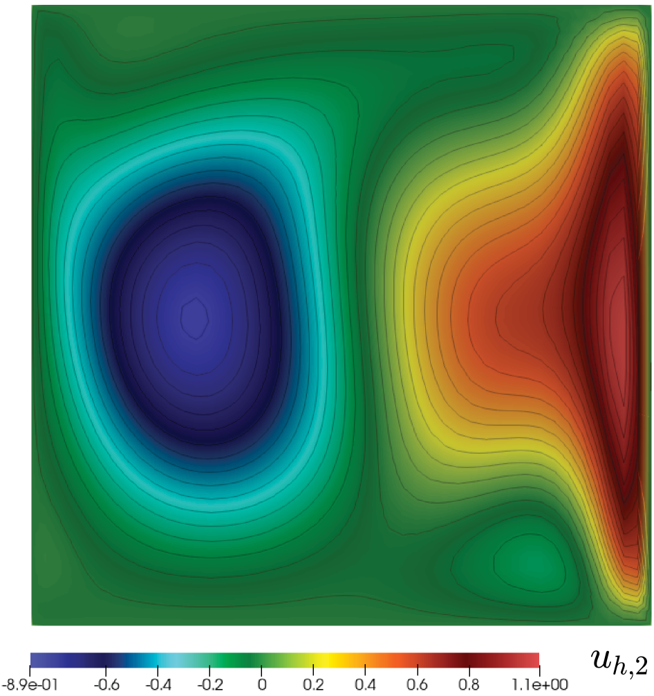
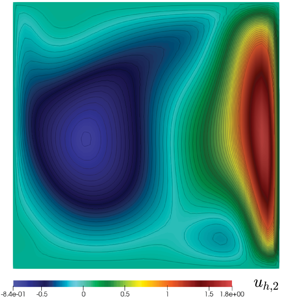
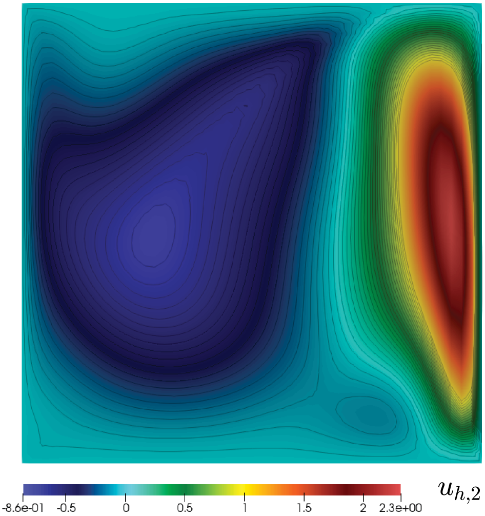
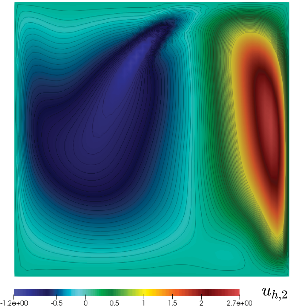
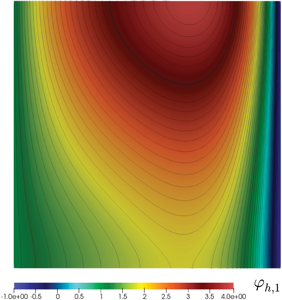
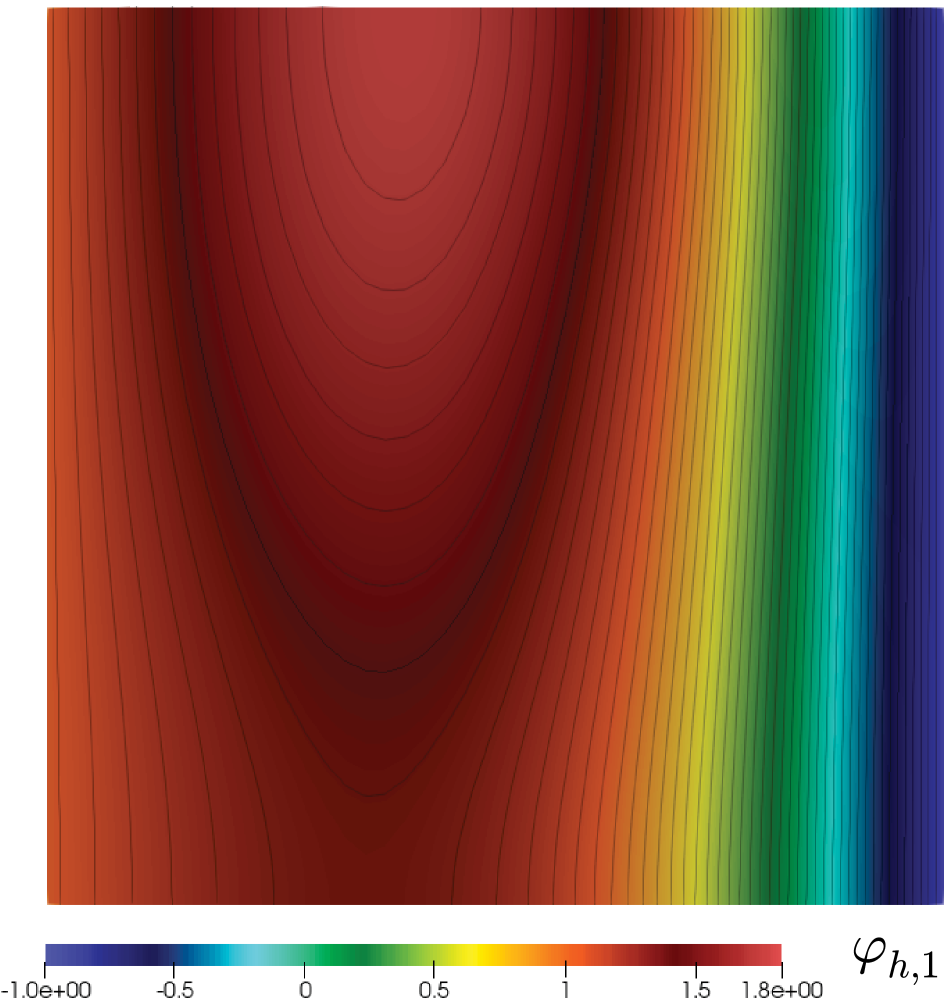
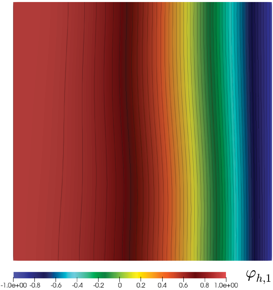
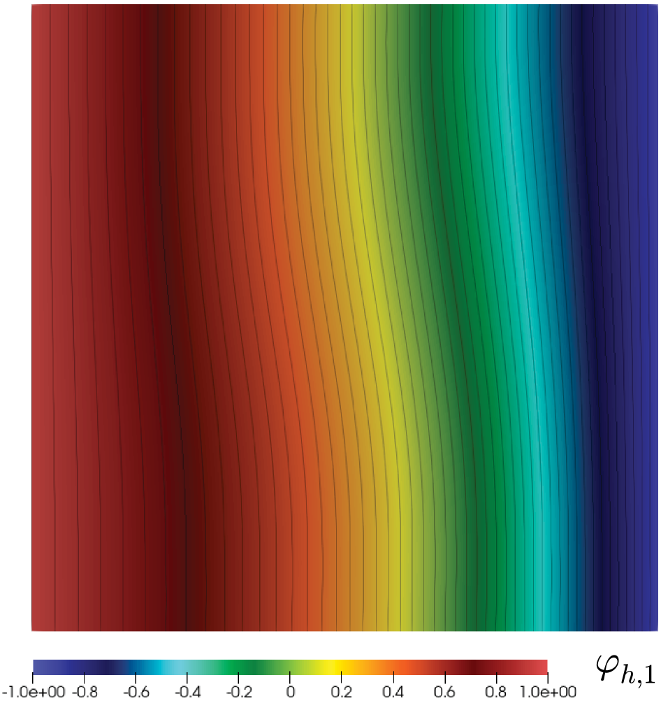
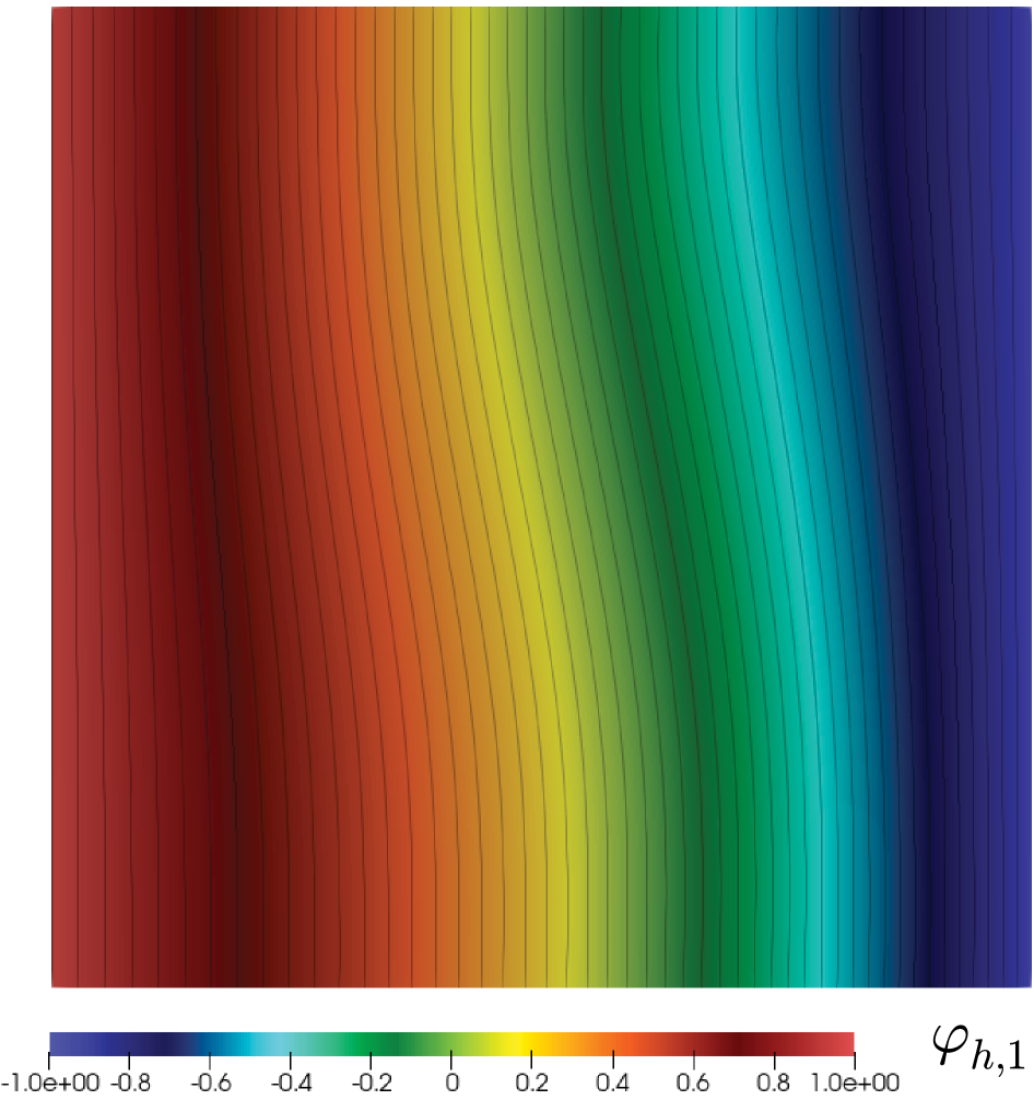
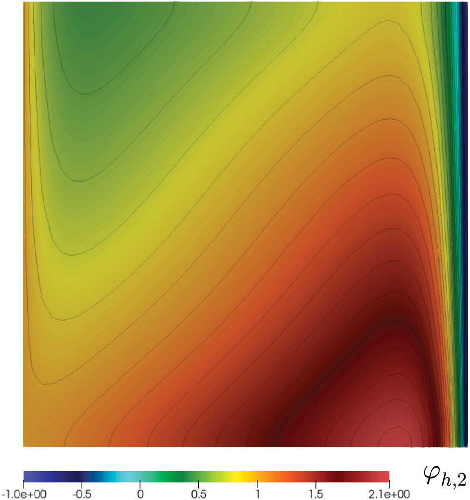
In Table 3, we summarize the convergence history, where we can note that the rate of convergence predicted by Theorem 5.5 is attained by all the unknowns for and time step . We mention that the errors and the convergence rates are computed by considering the discrete solution obtained with a finer mesh () as the exact solution. Additionally, in Figures 1 and 2, we display the approximation of the velocity components, temperature and concentration. All the figures presented there were obtained with degrees of freedom (used as exact solution) in the time step , with .
| 0.0707 | 5845 | 4.47e+01 | 1.07e+01 | 5.79e-01 | 5.15e-01 | 8.63e-01 | ||||||
| 0.0566 | 9055 | 3.57e+01 | 1.01 | 8.35e+00 | 1.10 | 4.54e-01 | 1.08 | 4.02e-01 | 1.12 | 6.86e-01 | 1.03 | |
| 0 | 0.0471 | 12965 | 2.95e+01 | 1.05 | 6.80e+00 | 1.13 | 3.61e-01 | 1.26 | 3.21e-01 | 1.24 | 5.66e-01 | 1.05 |
| 0.0404 | 17575 | 2.53e+01 | 0.99 | 5.72e+00 | 1.12 | 3.08e-01 | 1.03 | 2.70e-01 | 1.11 | 4.85e-01 | 1.01 | |
| 0.0354 | 22885 | 2.21e+01 | 1.03 | 4.93e+00 | 1.11 | 2.68e-01 | 1.02 | 2.34e-01 | 1.08 | 4.19e-01 | 1.09 |
References
- [1] J. Abedi, S. Aliabadi, Simulation of incompressible flows with heat and mass transfer using parallel finite element method. Electronic J. Diff. Eq., Conference 10 (2003), 1–11.
- [2] R.A. Adams and J.J.F. Fournier, Sobolev Spaces. Second edition. Pure and Applied Mathematics (Amsterdan), 140. Elsevier/Academic Press, Amsterdam, 2003.
- [3] G. Alekseev, D. Tereshko and V. Pukhnachev. Boundary control problems for Oberbeck-Boussinesq model of heat and mass transfer. Advanced Topics in Mass Transfer (2011), 485–512.
- [4] J.A. Almonacid, G.N. Gatica and R. Oyarzúa, A new mixed finite element method for the n-dimensional Boussinesq problem with temperature-dependent viscosity. Calcolo 55 (2018), no. 3, Art. 36, 42pp.
- [5] M. Alvarez, G.N. Gatica, B. Gómez-Vargas and R. Ruiz-Baier, New mixed finite element methods for natural convection with phase-change in porous media. J. Sci. Comput. 80 (2019), no. 1, 141–174.
- [6] M. Alvarez, G.N. Gatica and R. Ruiz-Baier, A mixed-primal element approximation of a sedimentation-consolidation system. M3AS: Math. Models Methods Appl. Sci., 26 (2016), no. 5, 867–900.
- [7] M. Alvarez, G.N. Gatica and R. Ruiz-Baier, An augmented mixed-primal finite element method for a coupled flow-transport problem. ESAIM Math. Model. Numer. Anal. 49 (2015), no. 5, 1399–1427.
- [8] M. Alvarez, G.N. Gatica, B. Gomez-Vargas, R. Ruiz-Baier, New Mixed Finite Element Nethods For Natural Convection with Phase-Change in Porous Media. Journal of Scientific Computing. vol. 80, 1, pp. 141-174, (2019).
- [9] F. Brezzi and M. Fortin, Mixed and Hybrid Finite Element Methods. Springer Series in Computational Mathematics, 15. Springer-Verlag, New York, 1991.
- [10] R. Bürger, P.E. Méndez and R. Ruiz-Baier, On H(div)-conforming methods for double-diffusion equations in porous media. SIAM J. Numer. Anal. 57 (2019), no. 3, 1318–1343.
- [11] E. Cáceres and G.N. Gatica, A mixed virtual element method for the pseudostress-velocity formulation of the Stokes problem. IMA J. Numer. Anal. 37 (2017), no. 1, 296–331.
- [12] J. Camaño, G.N. Gatica, R. Oyarzúa and G. Tierra, An augmented mixed finite element method for the Navier-Stokes equations with variable viscosity. SIAM J. Numer. Anal. 54 (2016), no. 2, 1069–1092.
- [13] S. Caucao, G. N. Gatica and R. Oyarzúa, Analysis of an augmented fully-mixed formulation for the coupling of the Stokes and heat equations. ESAIM Math. Model. Numer. Anal. 52 (2018), no. 5, 1947–1980.
- [14] Y.Y. Chen, B.W. Li and J.K. Zhang, Spectral collocation method for natural convection in a square porous cavity with local thermal equilibrium and non-equilibrium models. Int. J. Heat Mass Transfer 64 (2013), 35–49.
- [15] P. Cheng, Heat transfer in geothermal systems. Adv. Heat Transfer 14 (1979), 1–105.
- [16] P.G. Ciarlet, Linear and Nonlinear Functional Analysis with Applications. Society for Industrial and Applied Mathematics, Philadelphia, PA, 2013.
- [17] A. Çibik and S. Kaya, Finite element analysis of a projection-based stabilization method for the Darcy-Brinkman equations in double-diffusive convection. Appl. Numer. Math. 64 (2013), 35–49.
- [18] E. Colmenares, G.N. Gatica, S. Moraga and R. Ruiz-Baier, A fully-mixed finite element method for the steady state Oberbeck-Boussinesq system. SMAI J. Comput. Math. 6 (2020), 125–157.
- [19] E. Colmenares, G.N. Gatica and R. Oyarzúa, Fixed point strategies for mixed variational formulations of the stationary Boussinesq problem. C. R. Math. Acad. Sci. Paris 354 (2016), no. 1, 57–62.
- [20] E. Colmenares, G.N. Gatica and R. Oyarzúa, Analysis of an augmented mixed-primal formulation for the stationary Boussinesq problem. Numer. Methods Partial Differential Equations 32 (2016), no. 2, 445–478.
- [21] E. Colmenares, G.N. Gatica and R. Oyarzúa, An augmented fully-mixed finite element method for the stationary Boussinesq problem. Calcolo 54 (2017), no. 1, 167–205.
- [22] H. Dallmann and D. Arndt, Stabilized finite element methods for the Oberbeck-Boussinesq model. J. Sci. Comput. 69 (2016), no. 1, 244–273.
- [23] T.A. Davis, Algorithm 832: UMFPACK V4.3–an unsymmetric-pattern multifrontal method. ACM Trans. Math. Software 30 (2004), no. 2, 196–199.
- [24] B. Daya Reddy Introductory Functional Analysis: With Appliations to Boundary Value Problems and Finite Elements. Texts in Applied Mathematics, Springer (1998), no. 27.
- [25] A. Ern and J.L. Guermond, Theory and Practice of Finite Elements, Applied Mathematical Sciences, Springer (2004), no. 159.
- [26] L.E. Figueroa, G.N. Gatica and A. Márquez, Augmented mixed finite element methods for the stationary Stokes equations. SIAM J. Sci. Comput. 31 (2008/09), no. 2, 1082–1119.
- [27] G.N. Gatica, A Simple Introduction to the Mixed Finite Element Method. Theory and Applications. Springer Briefs in Mathematics. Springer, Cham, 2014.
- [28] G.N. Gatica, Introducción al Análisis Funcional. Teoría y Aplicaciones. Editorial Reverte, Barcelona Bogotá Buenos Aires Caracas México, 2014.
- [29] B. Gebhart and L. Pera, The nature of vertical natural convection flows resulting from the combined buoyancy effects of thermal and mass diffusion. Int. J. Heat Mass Transfer 14 (1971), no. 12, 2025–2050.
- [30] B. Gebhart and L. Pera, Natural convection flows adjacent to horizontal surfaces resulting from the combined buoyancy effects of thermal and mass diffusion. Int. J. Heat Mass Transfer 15 (1972), no. 2, 269–278.
- [31] C. Geuzaine and J.-F. Remacle, Gmsh: a three-dimensional finite element mesh generator with built-in pre- and post-processing facilities. Int. J. Numer. Methods Engrg. 79 (2009), no. 11, 1309–1331.
- [32] V. Girault and P-A. Raviart, Finite Element Methods for Navier-Stokes Equations. Theory and Algorithms. Springer Series in Computational Mathematics, 5. Springer-Verlag, Berlin, 1986.
- [33] J. Guzmán, F.A. Sequeira and C.W. Shu, H(div) conforming and DG methods for incompressible Euler’s equations. IMA J. Numer. Anal. 37 (2017), no. 4, 1733–1771.
- [34] M. Hammami, M. Mseddi and Mounir Baccar, Numerical Study of Coupled Heat and Mass Transfer in a Trapezoidal Cavity. Eng. Appl. Comput. Fluid Mech. 1 (2007), no. 3, 216–226.
- [35] M. Karimi-Fard, M.C. Charrier-Mojtabi and K. Vafai, Non-Darcian effects on double-diffusive convection within a porous medium. Numer. Heat Transfer, Part A: Appl. 31 (1997), no. 8, 837–852.
- [36] W. McLean, Strongly elliptic systems and boundary integral equations. Cambridge University Press, Cambridge, 2000.
- [37] A. Mojtabi and M.C. Charrier-Mojtabi, Double-diffusive convection in porous media. Handbook of Porous Media, Part III. Taylor and Francis, 2005.
- [38] N. Moraga, C. Zambra, P. Torres and R Lemus-Mondaca, Fluid dinamics, heat and mass transfer modelling by finite volume method for agrofood processes. DYNA 78 (2011), 140–149.
- [39] D.A. Nield and A. Bejan, Convection in porous media. Second edition. Springer Science and & Business Media. Springer-Verlag, New York, 1999.
- [40] R. Oyarzúa, T. Qin and D. Schötzau, An exactly divergence-free finite element method for a generalized Boussinesq problem. IMA J. Numer. Anal. 34 (2014), no. 3, 1104–1135.
- [41] A. Quarteroni and A. Valli. Numerical Approximation of Partial Differential Equations. Springer Series in Computational Mathematics, 23. Springer-Verlag, Berlin, 1994.
- [42] P.-A. Raviart and J.-M. Thomas, Introduction à l’Analyse Numérique des Équations aux Dérivées Partielles. (French) [Introduction to the numerical analysis of partial differential equations] Collection Mathématiques Appliquées pour la Maîtrise. Masson, Paris, 1983.
- [43] J.E. Roberts and J.-M. Thomas, Mixed and Hybrid Methods. Handbook of numerical analysis, vol. II, 523–639, Handb. Numer. Anal., II, North-Holland, Amsterdam, 1991.
- [44] S. C. Saha and A. Hossain, Natural convection flow with combined buoyancy effects due to thermal and mass diffusion in a thermally stratified media. Nonlinear Analysis: Modelling and Control 9 (2004), 89–102.
- [45] L.R. Scott and S. Zhang, Finite element interpolation of nonsmooth functions satisfying boundary conditions. Math. Comp. 54 (1990), no. 190, 483–493.