Enhancing Taxonomy Completion with Concept Generation via Fusing Relational Representations

Abstract.

A clear and well-documented LaTeX document is presented as an article formatted for publication by ACM in a conference proceedings or journal publication. Based on the “acmart” document class, this article presents and explains many of the common variations, as well as many of the formatting elements an author may use in the preparation of the documentation of their work.

Abstract.

Automatic construction of a taxonomy supports many applications in e-commerce, web search, and question answering. Existing taxonomy expansion or completion methods assume that new concepts have been accurately extracted and their embedding vectors learned from the text corpus. However, one critical and fundamental challenge in fixing the incompleteness of taxonomies is the incompleteness of the extracted concepts, especially for those whose names have multiple words and consequently low frequency in the corpus. To resolve the limitations of extraction-based methods, we propose GenTaxo to enhance taxonomy completion by identifying positions in existing taxonomies that need new concepts and then generating appropriate concept names. Instead of relying on the corpus for concept embeddings, GenTaxo learns the contextual embeddings from their surrounding graph-based and language-based relational information, and leverages the corpus for pre-training a concept name generator. Experimental results demonstrate that GenTaxo improves the completeness of taxonomies over existing methods.

1. Introduction

Taxonomies have been widely used to enhance the performance of many applications such as question answering (Yang et al., 2017; Yu et al., 2021) and personalized recommendation (Huang et al., 2019). With the influx of new content in evolving applications, it is necessary to curate these taxonomies to include emergent concepts; however, manual curation is labor-intensive and time-consuming. To this end, many recent studies aim to automatically expand or complete an existing taxonomy. For example, given a new concept, Shen et al. measured the likelihood of each existing concept in the taxonomy being its hypernym and then added it as a new leaf node (Shen et al., 2020). Manzoor et al. extended the measurement to be taxonomic relatedness with implicit relational semantics (Manzoor et al., 2020). Zhang et al. predicted the position of the new concept considering hypernyms and hyponyms (Zhang et al., 2021). In all of these cases, the distance between concepts was measured using their embeddings learned from some text corpus, with the underlying assumption that new concepts could be extracted accurately and found frequently in the corpus.

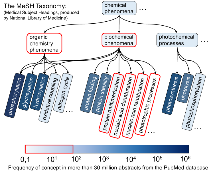
Figure 1. A great number of concepts that are desired to be in the taxonomies (e.g., MeSH) are very rare in even large-scale text corpus (e.g., 30 million PubMed abstracts). So it is hard to extract these concepts or learn their embedding vectors. Concept names need to be generated rather than extracted to fix the incompleteness of taxonomies.

We argue that such an assumption is inappropriate in real-world taxonomies based on the frequency of concepts in Medical Subject Headings (MeSH), a widely-used taxonomy of approximately 30,000 terms that is updated annually and manually, in a large-scale public text corpus of 30 million paper abstracts (about 6 billion tokens) from the PubMed database. We observe that many concepts that have multiple words appear fewer than 100 times in the corpus (as depicted by the red outlined nodes in Figure 1) and around half of the terms cannot be found in the corpus (see Table 1 in Section 4). Concept extraction tools (Zeng et al., 2020) often fail to find them at the top of a list of over half a million concept candidates; and there is insufficient data to learn their embedding vectors. The incompleteness of concepts is a critical challenge in taxonomy completion, and has not yet been properly studied.

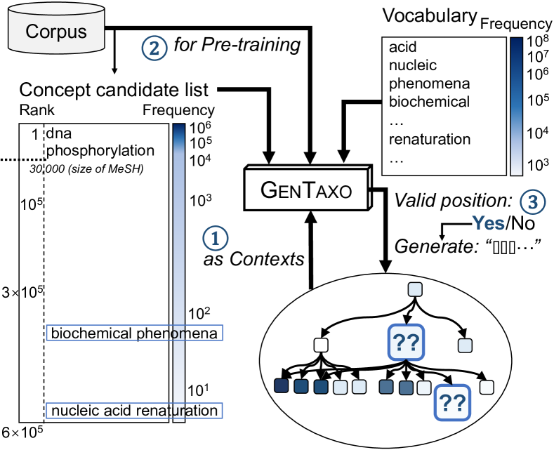
Figure 2. Existing methods extracted a concept candidate list from the corpus and assumed that the top concepts (high frequency or quality) could be added into existing taxonomies. However, frequent concepts may not be qualified and many qualified concepts are very rare. We find that though the concept names are not frequent, their tokens are. Our idea is to generate concept names at candidate positions with relational contexts to complete taxonomies. Our solution GenTaxo is pre-trained on the corpus and learns to generate the names token by token on the existing taxonomy.

Despite the low frequency of many multi-gram concepts in a text corpus, the frequency of individual words is naturally much higher. Inspired by recent advances in text generation (Meng et al., 2017; Yu et al., 2020b), we propose a new task, “taxonomy generation”, that identifies whether a new concept fits in a candidate position within an existing taxonomy, and if it does fit, generates the concept name token by token.

The key challenge lies in the lack of information for accurately generating the names of new concepts when their full names do not (frequently) appear in the text corpus. To address this challenge, our framework for enhancing taxonomy completion, called GenTaxo, has the following novel design features (see Figure 2 and 3):

First, GenTaxo has an encoder-decoder scheme that learns to generate any concept in the existing taxonomy in a self-supervised manner. Suppose an existing concept $v$ is masked. Two types of encoders are leveraged to fuse both sentence-based and graph-based representations of the masked position learned from the relational contexts. One is a sequence encoder that learns the last hidden states of a group of sentences that describe the relations such as “$v_{p}$ is a class of” and “$v_{c}$ is a subclass of”, when $v_{p}$ and $v_{c}$ are parent and child concepts of the position, respectively. The other is a graph encoder that aggregates information from two-hop neighborhoods in the top-down subgraph (with $v$ at the bottom) and bottom-up subgraph (with $v$ at the top). The fused representations are fed into a GRU-based decoder to generate $v$’s name token by token with a special token [EOS] at the end. With the context fusion, the decoding process can be considered as the completion of a group of sentences (e.g., “$v_{p}$ is a class of” and “$v_{c}$ is a subclass of”) with the same ending term while simultaneously creating a hyponym/hypernym node in the top-down/bottom-up subgraphs.

Second, GenTaxo is pre-trained on a large-scale corpus to predict tokens in concept names. The pre-training task is very similar to the popular Mask Token Prediction task (Devlin et al., 2019) except that the masked token must be a token of a concept that appears in the existing taxonomy and is found in a sentence of the corpus.

Third, GenTaxo performs the task of candidate position classification simultaneously with concept name generation. It has a binary classifier that uses the final state of the generated concept name to predict whether the concept is needed at the position. We adopt negative sampling to create “invalid” candidate positions in the existing taxonomy. The classifier is attached after the name generation (not before it) because the quality of the generated name indicates the need for a new concept at the position.

Furthermore, we develop GenTaxo++ to enhance extraction-based methods, when a set of new concepts, though incomplete, needs to be added to existing taxonomies (as described in existing studies). In GenTaxo++, we apply GenTaxo to generate concept names in order to expand the set of new concepts. We then use the extraction-based methods with the expanded set to improve the concept/taxonomy completeness.

The main contributions of this work are summarized as follows:

• We propose a new taxonomy completion task that identifies valid positions to add new concepts in existing taxonomies and generates their names token by token.

• We design a novel framework GenTaxo that has three novel designs: (1) an encoder-decoder scheme that fuses sentence-based and graph-based relational representations and learns to generate concept names; (2) a pre-training process for concept token prediction; and (3) a binary classifier to find valid candidate positions. Furthermore, GenTaxo++ is developed to enhance existing extraction-based methods with the generated concepts, when a set of new concepts are available.

• Experiments on six real-world taxonomy data sets demonstrate that (1) concept generation can significantly improve the recall and completeness of taxonomies; (2) even some concepts that do not appear in the corpus can be accurately generated token by token at valid positions; and (3) fusing two types of relational representations is effective.

2. Problem Definition

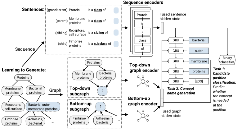
Figure 3. Architecture of GenTaxo. Suppose the concept “bacterial outer membrane proteins” is masked. Given the masked position in the taxonomy, the model learns to generate the name of the concept. It has two types of encoders to represent the relational contexts of the position. Sequence encoders learn a group of sentences that describe the relations with the masked concept. Graph encoders learn the masked concept’s embedding by aggregating information from its top-down and bottom-up subgraphs. The fused sentence- and graph-based hidden states are used to predict whether the masked position is valid (Task 1). They are fed into GRU decoders to generate the concept’s name (Task 2).

Traditionally, the input of the taxonomy completion task includes two parts (Manzoor et al., 2020; Shen et al., 2020; Yu et al., 2020a; Zhang et al., 2021): (1) an existing taxonomy $\mathcal{T}_{0}=(\mathcal{V}_{0},\mathcal{E}_{0})$ and (2) a set of new concepts $\mathcal{C}$ that have been either manually given or accurately extracted from text corpus $\mathcal{D}$. The overall goal is completing the existing taxonomy $\mathcal{T}_{0}$ into a larger one $\mathcal{T}=(\mathcal{V}_{0}\cup\mathcal{C},\mathcal{E}^{{}^{\prime}}$).

We argue that existing technologies, which defined the task as described above, could fail when concepts cannot be extracted due to their low frequency, or cannot be found in the corpus. We aim to mitigate this problem by generating the absent concepts to achieve better taxonomy completion performance. Suppose $v=(t_{1},t_{2},\dots,t_{T_{v}})$, where $t_{i}\in\mathcal{W}$ is the $i$-th token in the name of concept $v$, $T_{v}$ is the number of $v$’s tokens (length of $v$), $\mathcal{W}$ is the token vocabulary which includes words and punctuation marks (e.g., comma).

Definition 2.1 (Taxonomy).

We follow the definition of taxonomy in (Zhang et al., 2021). A taxonomy $\mathcal{T}=(\mathcal{V},\mathcal{E})$ is a directed acyclic graph where each node $v\in\mathcal{V}$ represents a concept (i.e., a word or a phrase) and each directed edge $\text{\textlangle}u,~{}v\text{\textrangle}\in\mathcal{E}$ implies a relation between a parent-child pair such as “is a type of” or “is a class of”. We expect the taxonomy to follow a hierarchical structure where concept $u$ is the most specific concept that is more general than concept $v$. Note that a taxonomy node may have multiple parents.

In most taxonomies, the parent-child relation can be specified as a hypernymy relation between concept $u$ and $v$, where $u$ is the hypernym (parent) and $v$ is the hyponym (child). We use the terms “hypernym” and “parent”, “hyponym” and “child” interchangeably throughout the paper.

Definition 2.2 (Candidate Position).

Given two sets of concepts $\mathcal{V}_{p},\mathcal{V}_{c}\subset\mathcal{V}_{0}$, if $v_{c}$ is one of the descendants of $v_{p}$ in the existing taxonomy for any pair of concepts $v_{p}\in\mathcal{V}_{p}$ and $v_{c}\in\mathcal{V}_{c}$, then a candidate position acts as a placeholder for a new concept $v$. It becomes a valid position when $v$ satisfies (1) $v_{p}$ is a parent of $v$ and (2) $v_{c}$ is a child of $v$. When it is a valid position, we add edges $\text{\textlangle}v_{p},~{}v\text{\textrangle}$ and $\text{\textlangle}v,~{}v_{c}\text{\textrangle}$ and delete redundant edges to update $\mathcal{E}^{{}^{\prime}}$.

We reduce the task of generating concept names for taxonomy completion as the problem below: Given text corpus $\mathcal{D}$ and a candidate position on an existing taxonomy $\mathcal{T}_{0}$, predict whether the position is valid, and if yes, generate the name of the concept $v$ from the token vocabulary $\mathcal{W}$ (extracted from $\mathcal{D}$) to fill in the position.

3. GenTaxo: Generate Concept Names

Overall architecture

Figure 3 presents the architecture of GenTaxo. The goal is to learn from an existing taxonomy to identify valid candidate positions and generate concept names at those positions. Given a taxonomy, it determines valid candidate positions by masking an existing concept in the taxonomy; it also determines invalid candidate positions using negative sampling strategies which will be discussed in Section 3.2.

Here we focus on the valid positions and masked concepts. As shown in the left bottom side of Figure 3, suppose the term “bacterial outer membrane proteins” is masked. GenTaxo adopts an encoder-decoder scheme in which the encoders represent the taxonomic relations in forms of sentences and subgraphs (see the middle part of the figure) and the decoders perform two tasks to achieve the goal (see the right-hand side of the figure).

3.1. Encoders: Representing Taxonomic Relations

Here we introduce how to represent the taxonomic relations into sentences and subgraphs, and use sequence and graph encoders to generate and fuse the relational representations.

3.1.1. Representing Taxonomic Relations as Sentences

Given a taxonomy $\mathcal{T}_{0}=(\mathcal{V}_{0},\mathcal{E}_{0})$ and a candidate position for masked concept $v$, we focus on three types of taxonomic relations between the masked concept $v$ and some concepts $u\in\mathcal{V}_{0}$:

1. Parent or ancestor. Suppose there is a sequence of nodes $(v_{1},v_{2},\dots,v_{l})$ where $v_{1}=u$, $v_{l}=v$, and $\text{\textlangle}v_{i},~{}v_{i+1}\text{\textrangle}\in\mathcal{E}_{0}$ for any $i=1,\dots,l-1$. In other words, there is a path from $u$ to $v$ in $\mathcal{T}_{0}$. When $l=1$, $u$ is a parent of $v$; when $l\geq 2$, $u$ is an ancestor. We denote $u=(t_{1},t_{2},\dots,t_{T_{u}})$, where $T_{u}$ is the length of concept $u$ and $\{t_{i}\}^{T_{u}}_{i=1}$ are its tokens. Then we create a sentence with the template below:

   “$t_{1}$ $t_{2}$ $\dots$ $t_{T_{u}}$ is a class of [MASK]”

   And we denote the set of parent or ancestor nodes of $v$ (i.e., all possible $u$ as described above) by $\mathcal{V}_{p}(v)$.

2. Child or descendant. Similar as above expect $v_{1}=v$ and $v_{l}=u$, we have a path from $v$ to $u$. When $l=1$, $u$ is a child of $v$; when $l\geq 2$, $u$ is a descendant. Then we create a sentence:

   “$t_{1}$ $t_{2}$ $\dots$ $t_{T_{u}}$ is a subclass of [MASK]”

   We denote the set of child or descendant nodes of $v$ by $\mathcal{V}_{c}(v)$.

3. Sibling. If there is a concept $p\in\mathcal{V}_{0}$ and two edges $\text{\textlangle}p,~{}v\text{\textrangle}$ and $\text{\textlangle}p,~{}u\text{\textrangle}$, then $u$ is a sibling node of $v$. We create a sentence:

   “$t_{1}$ $t_{2}$ $\dots$ $t_{T_{u}}$ is a sibling of [MASK]”

Given the candidate position for concept $v$, we can collect a set of sentences from its relational contexts, denoted by $\mathcal{S}(v)$. We apply neural network models that capture sequential patterns in the sentences and create the hidden states at the masked position. The hidden states are vectors that encode the related concept node $u$ and the relational phrase to indicate the masked concept $v$. The hidden states support the tasks of concept name generation and candidate position classification. We provide three options of sentence encoders: BiGRU, Transformer, and SciBERT (Beltagy et al., 2019).

3.1.2. Representing Taxonomic Relations as Subgraphs

The relations between the masked concept $v$ and its surrounding nodes can be represented as two types of subgraphs:

1. Top-down subgraph: It consists of all parent and ancestor nodes of $v$, denoted by $G_{\text{down}}(v)=\{\mathcal{V}_{\text{down}}(v),\mathcal{E}_{\text{down}}(v)\}$, where $\mathcal{V}_{\text{down}}(v)=\mathcal{V}_{p}(v)$ and $\mathcal{E}_{\text{down}}(v)=\{\text{\textlangle}v_{i},~{}v_{j}\text{\textrangle}\in\mathcal{E}\mid v_{i},v_{j}\in\mathcal{V}_{\text{down}}(v)\}$. The role of $v$ is the very specific concept of any other concepts in this subgraph. So, the vector representations of this masked position should be aggregated in a top-down direction. The aggregation indicates the relationship of being from more general to more specific.

2. Bottom-up subgraph: Similarly, it consists of all child and descendant nodes of $v$, denoted by $G_{\text{up}}(v)=\{\mathcal{V}_{\text{up}}(v),\mathcal{E}_{\text{up}}(v)\}$, where $\mathcal{V}_{\text{up}}(v)=\mathcal{V}_{c}(v)$ and $\mathcal{E}_{\text{up}}(v)=\{\text{\textlangle}v_{i},~{}v_{j}\text{\textrangle}\in\mathcal{E}\mid v_{i},v_{j}\in\mathcal{V}_{\text{up}}(v)\}$. The representations of this masked position should be aggregated in a bottom-up direction. The aggregation indicates the relationship of being from specific to general.

Graph encoders:

We adopt two independent graph neural networks (GNNs) to encode the relational contexts in $G_{\text{down}}(v)$ and $G_{\text{up}}(v)$ separately. Given a subgraph $G$, GNN learns the graph-based hidden state of every node on the final layer through the graph structure, while we will use that of the node $v$ for next steps.

$v$ was specifically denoted for the masked concept node. In this paragraph, we denote any node on $G$ by $v$ for convenience. We initialize the vector representations of $v$ randomly, denoted by $\mathbf{v}^{(0)}$. Then, the $K$-layered GNN runs the following functions to generate the representations of $v$ on the $k$-th layer ($k=1,\dots,K$):

$$\mathbf{a}^{(k-1)} = \textsc{Aggregate}_{k}(\big{\{}(\mathbf{u}^{(k-1)}):\forall u\in\mathcal{N}(v)\cup G\big{\}}),$$

$$\mathbf{v}^{(k)} = \textsc{Combine}_{k}(\mathbf{v}^{(k-1)},\mathbf{a}^{(k-1)}),$$

where $\mathcal{N}(v)$ is the set of neighbors of $v$ in $G$.

There are a variety of choices for $\textsc{Aggregate}_{k}(\cdot)$ and $\textsc{Combine}_{k}(\cdot)$. For example, $\textsc{Aggregate}_{k}(\cdot)$ can be mean pooling, max pooling, graph attention, and concatenation (Koncel-Kedziorski et al., 2019; Hamilton et al., 2017). One popular choice for $\textsc{Combine}_{k}(\cdot)$ is graph convolution: $\mathbf{v}^{(k)}=\sigma\left(\mathbf{W}^{(k)}(\mathbf{v}^{(k-1)}\oplus\mathbf{a}^{(k-1)})\right)$, where $\mathbf{W}^{(k)}$ is the weight matrix for linear transformation on the $k$-th layer and $\sigma(\cdot)$ is a nonlinear function.

For the masked concept $v$, we finally return the graph-based hidden state $\mathbf{v}_{G}$ at K-th layer, i.e., $\mathbf{v}_{G}=\mathbf{v}^{(K)}$.

3.1.3. Representations Fusion

As aforementioned, we have a set of sentence-based hidden states $\{\mathbf{h}(s)\}_{s\in\mathcal{S}(v)}$ from the sentence encoder; also, we have two graph-based hidden states $\mathbf{v}_{G_{\text{down}}}$ and $\mathbf{v}_{G_{\text{up}}}$ from the graph encoder. In this section, we present how to fuse these relational representations for decoding concept names.

Fusing sentence-based hidden states:

We use the self-attention mechanism to fuse the hidden states with a weight matrix $\mathbf{W}_{\text{seq}}$:

$$\mathbf{h}_{\text{seq}}=\sum_{s\in\mathcal{S}(v)}w(s)\cdot\mathbf{h}(s),~{}\text{where}~{}w(s)=\frac{\exp(\sigma(\mathbf{W}_{\text{seq}}\mathbf{h}(s)))}{\sum\limits_{s^{\prime}\in\mathcal{S}(v)}\exp(\sigma(\mathbf{W}_{\text{seq}}\mathbf{h}(s^{\prime})))}.$$

Fusing graph-based hidden states:

We adopt a learnable weighted sum to fuse $\mathbf{v}_{G_{\text{down}}}$ and $\mathbf{v}_{G_{\text{up}}}$ with weight matrices $\mathbf{W}_{\text{down}}$ and $\mathbf{W}_{\text{up}}$:

$$\mathbf{v}_{\text{graph}}=\beta\cdot\mathbf{v}_{G_{\text{down}}}+(1-\beta)\cdot\mathbf{v}_{G_{\text{up}}},$$

where $\beta=\frac{\exp(\sigma(\mathbf{W}_{\text{down}}\cdot\mathbf{v}_{G_{\text{down}}}))}{\exp(\sigma(\mathbf{W}_{\text{down}}\cdot\mathbf{v}_{G_{\text{down}}}))+\exp(\sigma(\mathbf{W}_{\text{up}}\cdot\mathbf{v}_{G_{\text{up}}}))}$.

Fusing the fused sentence- and graph-based hidden states:

Given a masked concept $v$, there are a variety of strategies to fuse $\mathbf{h}_{\text{seq}}$ and $\mathbf{v}_{\text{graph}}$: $\mathbf{v}_{\text{fuse}}=\textsc{Fuse}(\mathbf{h}_{\text{seq}},\mathbf{v}_{\text{graph}})$, such as mean pooling, max pooling, attention, and concatenation. Take concatenation as an example: $\textsc{Fuse}(\mathbf{a},\mathbf{b})=\mathbf{a}\oplus\mathbf{b}$.

3.2. Decoders: Identifying Valid Positions and Generating Concept Names

Given a masked position $v$, we now have the fused representations of its relational contexts $\mathbf{v}_{\text{fuse}}$ from the above encoders. We perform two tasks jointly to complete the taxonomy: one is to identify whether the candidate position is valid or not; the other is to generate the name of concept for the masked position.

3.2.1. Task 1: Candidate Position Classification

Given a candidate position, this task predicts whether it is valid, i.e., a concept is needed. If the position has a masked concept in the existing taxonomy, it is a valid position; otherwise, this invalid position is produced by negative sampling. We use a three-layer feed forward neural network (FFNN) to estimate the probability of being a valid position with the fused representations: $p_{\text{valid}}(v)=\textsc{FFNN}(\mathbf{v}_{\text{fuse}})$. The loss term on the particular position $v$ is based on cross entropy:

$$L_{1}(\Theta;v)=-(y_{v}\cdot\log(p_{\text{valid}}(v))+(1-y_{v})\cdot\log(1-p_{\text{valid}}(v))),$$

where $y_{v}=1$ when $v$ is valid as observed; otherwise, $y_{v}=0$.

Negative sampling:

Suppose a valid position is sampled by masking an existing concept $v\in\mathcal{V}_{0}$, whose set of parent/ancestor nodes is denoted by $\mathcal{V}_{p}(v)$ and set of child/descendant nodes is denoted by $\mathcal{V}_{c}(v)$. We create $r_{\text{neg}}$ negative samples (i.e., invalid positions) by replacing one concept in either $\mathcal{V}_{p}(v)$ or $\mathcal{V}_{c}(v)$ by a random concept in $\mathcal{V}_{\text{neg}}(v)=\mathcal{V}_{0}\setminus(\mathcal{V}_{p}(v)\cup\mathcal{V}_{c}(v)\cup\{v\})$. We will investigate the effect of negative sampling ratio $r_{\text{neg}}$ in experiments.

3.2.2. Task 2: Concept Name Generation

We use a Gated Recurrent Unit (GRU)-based decoder to generate the name of concept token by token which is a variable-length sequence $v=(v_{1},v_{2},\dots,v_{T_{v}})$. As shown at the right of Figure 3, we add a special token [EOS] to indicate the concept generation is finished.

We initialize the hidden state of the decoder as $\mathbf{v}_{0}=\mathbf{h}_{\text{seq}}$. Then the conditional language model works as below:

$$\mathbf{v}_{t}=\textsc{GRU}(v_{t-1},\mathbf{v}_{t-1}\oplus\mathbf{v}_{\text{graph}}),$$

$$p(v_{t}|v_{t-1},\dots,v_{1},\mathbf{v}_{\text{fuse}})=\textsc{Readout}(v_{t-1},\mathbf{v}_{t},\mathbf{v}_{\text{fuse}}),$$

where $\textsc{Readout}(\cdot)$ is a nonlinear multi-layer function that predicts the probability of token $v_{t}$. Then this task can be regarded as a sequential multi-class classification problem. The loss term is:

$$L_{2}(\Theta;v)=-\log(p(v|\mathbf{v}_{\text{fuse}}))=-\sum^{T_{v}}_{t=1}\log(p(v_{t}|v_{<t},\mathbf{v}_{\text{fuse}})),$$

where $v$ is the target sequence (i.e., the concept name) and $\mathbf{v}_{\text{fuse}}$ is the fused relational representations of the masked position.

Pre-training:

To perform well in Task 2, a model needs the ability of predicting tokens in a concept’s name. So, we pre-train the model with the task of predicting masked concept’s tokens (MCT) in sentences of text corpus $\mathcal{D}$. We find all the sentences in $\mathcal{D}$ that contain at least one concept in the existing taxonomy $\mathcal{T}_{0}$. Given a sentence $X=(x_{1},x_{2},\dots,x_{n})$ where $(x_{s},\dots,x_{e})=v=(v_{1},\dots,v_{T_{v}})$ is an existing concept. Here a token $x_{m}$ is masked ($s\leq m\leq e$) and predicted using all past and future tokens. The loss function is:

$$L_{\text{MCT}}(\Theta;x_{m})=-\log(p(x_{m}|x_{1},\dots,x_{m-1},x_{m+1},\dots,x_{n})).$$

3.2.3. Joint Training

The joint loss function is a weighted sum of the loss terms of the above two tasks:

$$L=\sum_{v\in\mathcal{V}_{0}}\left(L_{1}(\Theta;v)+\lambda L_{2}(\Theta;v)\right)+\sum^{r_{\text{neg}}}_{i=1}\mathbb{E}_{v_{\text{neg}}\sim\mathcal{V}_{\text{neg}}(v)}L_{1}(\Theta;v_{\text{neg}}),$$

where $\lambda$ is introduced as a hyper-parameter to control the importance of Task 2 concept name generation.

3.3. GenTaxo++: Enhancing Extraction-based Methods with GenTaxo

While GenTaxo is designed to replace the process of extracting new concepts by concept generation, GenTaxo++ is an alternative solution when the set of new concepts is given and of high quality. GenTaxo++ can use any extraction-based method (Shen et al., 2020; Shang et al., 2020b; Shang et al., 2020a; Zhang et al., 2018, 2021; Manzoor et al., 2020; Yu et al., 2020a; Wang et al., 2021) as the main framework and iteratively expand the set of new concepts using concept generation (i.e., GenTaxo) to continuously improve the taxonomy completeness. We choose TaxoExpan as the extraction-based method GenTaxo++ (Shen et al., 2020).

The details of GenTaxo++ are as follows. We start with an existing taxonomy $T_{0}=(\mathcal{V}_{0},\mathcal{E}_{0})$ and a given set of new concepts $C_{0}$. During the $i$-th iteration, we first use GenTaxo to generate a set of new concepts, and then expand the set of new concepts and use the extraction-based method to update the taxonomy ($i\geq 1$):

$${T^{\prime}}_{i-1}=(\mathcal{V^{\prime}}_{i-1},\mathcal{E^{\prime}}_{i-1}) \leftarrow \textsc{GenTaxo}(T_{i-1}),$$

$$C_{i} = (C_{i-1}\cup\mathcal{V^{\prime}}_{i-1})\setminus\mathcal{V}_{i-1},$$

$$T_{i} \leftarrow \textsc{ExtractionMethod}(T_{i-1},C_{i}).$$

The iterative procedure terminates when $C_{i}==\emptyset$. In this procedure, we have two hyperparameters:

1. Concept quality threshold $\tau$: GenTaxo predicts the probability of being a valid position $p_{\text{valid}}(v)$ which can be considered as the quality of the generated concept $v$. We have a constraint on adding generated concepts to the set: $p_{\text{valid}}(v)\geq\tau$, for any $v\in C_{i}$. When $\tau$ is bigger, the process is more cautious: fewer concepts are added each iteration.

2. Maximum number of iterations ${max}_{\text{iter}}$: An earlier stop is more cautious but may cause the issue of low recall.

4. Experimental Settings

In this work, we propose GenTaxo and GenTaxo++ to complete taxonomies through concept generation. We conduct experiments to answer the following research questions (RQs):

• RQ1: Do the proposed approaches perform better than existing methods on taxonomy completion?

• RQ2: Given valid positions in an existing taxonomy and a corresponding large text corpus, which method produce more accurate concept names, the proposed concept generation or existing extraction-and-filling methods?

• RQ3: How do the components and hyperparametersa impact the performance of GenTaxo?

#Concepts #Tokens #Edges Depth Computer Science domains (Corpus: DBLP) MAG-CS 29,484 16,398 46,144 6 (found in corpus) 18,338 (62.2%) 13,914 (84.9%) OSConcepts 984 967 1,041 4 DroneTaxo 263 247 528 4 Biology/Biomedicine domains: (Corpus: PubMed) MeSH 29,758 22,367 40,186 15 (found in corpus) 14,164 (47.6%) 22,193 (99.2%) SemEval-Sci 429 573 452 8 SemEval-Env 261 317 261 6

Table 1. Statistics of six taxonomy data sets.

4.1. Datasets

Table 1 presents the statistics of six taxonomies from two different domains we use to evaluate the taxonomy completion methods:

• MAG-CS (Sinha et al., 2015): The Microsoft Academic Graph (MAG) taxonomy has over 660 thousand scientific concepts and more than 700 thousand taxonomic relations. We follow the processing in TaxoExpan (Shen et al., 2020) to select a partial taxonomy under the “computer science” (CS) node.

• OSConcepts (Peterson and Silberschatz, 1985): It is a taxonomy manually crated in a popular textbook “Operating System Concepts” for OS courses.

• DroneTaxo: is a human-curated hierarchical ontology on unmanned aerial vehicle (UAV).

• MeSH (Lipscomb, 2000): It is a taxonomy of medical and biological terms suggested by the National Library of Medicine (NLM).

• SemEval-Sci and SemEval-Env (Bordea et al., 2016): They are from the shared task of taxonomy construction in SemEval2016. We select two scientific-domain taxonomies (“science” and “environment”). Both datasets have been used in (Yu et al., 2020a; Wang et al., 2021).

We use two different corpora for the two different domains of data: (1) DBLP corpus has about 156K paper abstracts from the computer science bibliography website; (2) PubMed corpus has around 30M abstracts on MEDLINE. We observe that on the two largest taxonomies, around a half of concept names and a much higher percentage of unique tokens can found at least once in the corpus, which indicates a chance of generating rare concept names token by token. The smaller taxonomies show similar patterns.

MeSH:	Acc	Acc-Uni	Acc-Multi
HiExpan (Shen et al., 2018)	9.89	18.28	8.49
TaxoExpan (Shen et al., 2020)	16.32	28.35	14.31
Graph2Taxo (Shang et al., 2020a)	10.35	19.02	8.90
STEAM (Yu et al., 2020a)	17.04	27.61	15.26
ARBORIST (Manzoor et al., 2020)	16.01	27.91	14.19
TMN (Zhang et al., 2021)	16.53	27.52	14.85
GenTaxo ($r_{\text{neg}}=0$)	26.72	28.13	26.29
GenTaxo ($r_{\text{neg}}=0.15$)	26.93	31.34	26.07

Table 2. Evaluating the quality of generated concepts (RQ2).

4.2. Evaluation Methods

We randomly divide the set of concepts of each taxonomy into training, validation, and test sets at a ratio of 3:1:1. We build “existing” taxonomies with the training sets following the same method in (Zhang et al., 2021). To answer RQ1, we use Precision, Recall, and F1 score to evaluate the completeness of taxonomy. The Precision is calculated by dividing the number of correctly inserted concepts by the number of total inserted concepts, and Recall is calculated by dividing the the number of correct inserted concepts by the number of total concepts. For RQ2, we use accuracy (Acc) to evaluate the quality of generated concepts. For IE models, we evaluate what percent of concepts in taxonomy can be correctly extracted/generated when a position is given. We use Uni-grams (Acc-Uni), and Accuracy on Multi-grams (Acc-Multi) for scenarios where dataset contains only Uni-grams and multi-gram concepts.

Largest	MAG-CS			MeSH
two:	P	R	F1	P	R	F1
HiExpan	19.61	8.23	11.59	17.77	5.66	8.59
TaxoExpan	36.19	20.20	25.92	26.87	11.79	16.39
Graph2Taxo	23.43	12.97	16.70	26.13	10.35	14.83
STEAM	36.73	23.42	28.60	26.05	11.23	15.69
ARBORIST	29.72	15.90	20.72	26.19	10.76	15.25
TMN	28.82	23.09	25.64	23.73	9.84	13.91
GenTaxo	36.15	28.19	31.67	21.47	17.10	19.03
GenTaxo++	36.24	28.68	32.01	22.61	17.66	19.83
Computer	OSConcepts			DroneTaxo
Science:	P	R	F1	P	R	F1
HiExpan	21.77	13.71	16.82	43.24	30.77	35.95
TaxoExpan	30.43	21.32	25.07	60.98	48.08	53.77
Graph2Taxo	22.88	13.71	17.15	44.90	23.31	30.69
STEAM	30.71	19.79	24.07	58.33	53.85	56.00
ARBORIST	31.09	18.78	23.42	52.38	42.31	46.81
TMN	30.65	19.29	23.68	47.72	40.38	43.74
GenTaxo	18.32	12.18	14.63	11.63	9.62	10.53
GenTaxo++	30.18	25.89	27.87	65.96	59.62	62.63
Biology/	SemEval-Sci			SemEval-Env
Biomedicine:	P	R	F1	P	R	F1
HiExpan	14.63	10.34	12.12	15.79	8.11	10.72
TaxoExpan	24.14	29.17	26.42	23.07	16.22	19.05
Graph2Taxo	26.19	18.96	21.99	21.05	10.81	14.28
STEAM	35.56	27.58	31.07	46.43	35.13	39.99
ARBORIST	41.93	22.41	29.21	46.15	32.43	38.09
TMN	34.15	24.14	28.29	37.93	29.73	33.33
GenTaxo	11.43	6.90	8.61	16.13	13.51	14.70
GenTaxo++	38.78	32.76	35.52	48.28	37.84	42.42

Table 3. Performance on taxonomy completion: Bold for the highest among all. Underlined for the best baseline. (RQ1)

4.3. Baselines

This work proposes the first method that generates concepts for taxonomy completion. Therefore, We compare GenTaxo and GenTaxo++ with state-of-the-art extraction-based methods below:

• HiExpan (Shen et al., 2018) uses textual patterns and distributional similarities to capture the “isA” relations and then organize the extracted concept pairs into a DAG as the output taxonomy.

• TaxoExpan (Shen et al., 2020) adopts GNNs to encode the positional information and uses a linear layer to identify whether the candidate concept is the parent of the query concept.

• Graph2Taxo (Shang et al., 2020a) uses cross-domain graph structure and constraint-based DAG learning for taxonomy construction.

• STEAM (Yu et al., 2020a) models the mini-path information to capture global structure information to expand the taxonomy.

• ARBORIST (Manzoor et al., 2020) is the state-of-the-art method for taxonomy expansion. It aims for taxonomies with heterogeneous edge semantics and adopts a large-margin ranking loss to guaranteed an upper-bound on the shortest-path distance between the predicted parents and actual parents.

• TMN (Zhang et al., 2021) is the state-of-the-art method for taxonomy completion. It uses a triplet matching network to match a query concept with (hypernym, hyponym)-pairs.

For RQ1, the extraction-based baselines as well as GenTaxo++ are offered the concepts from the test set if they can be extracted from the text corpus but NOT to the pure generation-based GenTaxo. For RQ2, given a valid position in an existing taxonomy, it is considered as accurate if a baseline can extract the desired concept from text corpus and assign it to that position or if GenTaxo can generate the concept’s name correctly.

5. Experimental Results

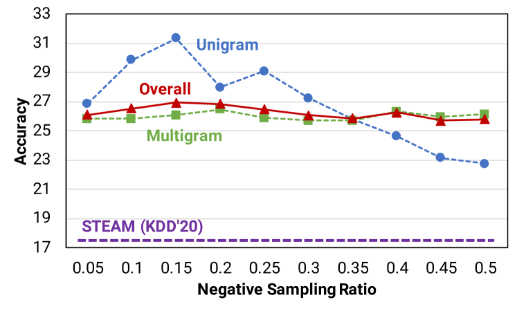
Figure 4. Effect of negative sampling ratio $r_{\text{neg}}$ on the quality of concept name generation.

5.1. RQ1: Taxonomy Completion

Table 3 presents the results on taxonomy completion. We have three main observations. First, TaxoExpan and STEAM are either the best or the second best among all the baselines on the six datasets. When TaxoExpan is better, the gap between the two methods in terms of F1 score is no bigger than 0.7% (15.69 vs 16.39 on MeSH); when STEAM is better, its F1 score is at least 2.2% higher than TaxoExpan (e.g., 28.60 vs 25.92 on MAG-CS). So, STEAM is generally a stronger baseline. This is because the sequential model that encodes the mini-paths from the root node to the leaf node learns useful information. The sequence encoders in our GenTaxo learn such information from the template-based sentences. STEAM loses to TaxoExpan on MeSH and OSConcepts due to the over-smoothing issue of too long mini-paths. We also find that ARBORIST and TMN do not perform better than STEAM. This indicates that GNN-based encoder in STEAM captures more structural information (e.g., sibling relations) than ARBORIST’s shortest-path distance and TMN’s scoring function based on hypernym-hyponym pairs.

Second, on the largest two taxonomies MAG-CS and MeSH, GenTaxo outperforms the best extraction-based methods STEAM and TaxoExpan in terms of recall and F1 score. This is because with the module of concept generation, GenTaxo can produce more desired concepts beyond those that are extracted from the corpus. Moreover, GenTaxo uses the fused representations of relational contexts. Compared with STEAM, GenTaxo encodes both top-down and bottom-up subgraphs. When TaxoExpan considers one-hop ego-nets of a query concept, GenTaxo aggregates multi-hop information into the fused hidden states.

Third, on the smaller taxonomies GenTaxo performs extremely bad due to the insufficient amount of training data (i.e., fewer than 600 concepts). Note that we assumed the set of new concepts was given for all the extraction-based methods, while GenTaxo was not given it and had to rely on name generation to “create” the set. In a fair setting – when we allow GenTaxo to use the set of new concepts, then we have – GenTaxo++ performs consistently better than all the baselines. This is because it takes advantages of both the concept generation and extraction-and-fill methodologies.

MeSH:	PT	1 hop	+ 2 hops		+ 3 hops
(F1 score)			Sibling	Grand-p/c
GRU	$\times$	18.19	18.29	18.92	17.41
	$\checkmark$	18.35	19.03	18.40	17.49
Transformer	$\times$	17.89	18.13	17.97	17.04
(Vaswani et al., 2017)	$\checkmark$	18.02	18.53	18.19	17.07
SciBERT	$\times$	18.05	18.16	18.12	17.29
(Beltagy et al., 2019)	$\checkmark$	18.11	18.87	18.23	17.41

Table 4. Ablation study on sequence encoders for sentence-based relational contexts. (PT is for Pre-training. Grand-p/c is for grandparent/grandchild.)

5.2. RQ2: Concept Name Generation

Table 2 presents the results on concept name generation/extraction: Given a valid position on an existing taxonomy, evaluate the accuracy of the concept names that are (1) extracted and filled by baselines or (2) generated by GenTaxo. Our observations are:

First, among all baselines, STEAM achieves the highest on multi-gram concepts, and TaxoExpan achieves the highest accuracy on uni-gram concepts. This is because the mini-path from root to leaf may encode the naming system for a multi-gram leaf node.

Second, the accuracy scores of TaxoExpan, STEAM, ARBORIST, and TMN are not significantly different from each other (within 1.03%). This indicates that these extraction-based methods are unfortunately limited by the presence of concepts in corpus.

Third, compared GenTaxo (the last two lines in the table) with STEAM, we find GenTaxo achieves 9.7% higher accuracy. This is because GenTaxo can assemble frequent tokens into infrequent or even unseen concepts.

Then, do negative samples help learn to generate concept names? In Figure 4, we show the accuracy of GenTaxo given different values of negative sampling ratio $r_{\text{neg}}$.

First, We observe that GenTaxo performs consistently better than the strongest baseline STEAM in this case. And the overall accuracy achieves the highest when $r_{\text{neg}}=0.15$. From our point of view, the negative samples accelerate the convergence at early stage by providing a better gradient descending direction for loss function. However, too many negative samples would weaken the signal from positive examples, making it difficult for the model to learn knowledge from them.

Second, we find that the uni-gram and multi-gram concepts have different kinds of sensitivity to the ratio but comply to the same trend. Generally uni-grams have higher accuracy because generating fewer tokens is naturally an easier task; however, they take a smaller percentage of the data. So the overall performance is closer to that on multi-grams. And our GenTaxo focuses on generating new multi-gram concepts.

MeSH: (F1 score)	U/D	1 hop	+ 2 hops	+ 3 hops
GAT (Veličković et al., 2018)	U	18.17	18.43	17.11
	D	18.29	18.94	17.39
GCN (Kipf and Welling, 2016)	U	18.10	18.27	17.09
	D	18.21	18.35	17.15
GraphSAGE (Hamilton et al., 2017)	U	18.12	18.36	17.05
	D	18.19	18.66	17.20
GraphTransformer (Koncel-Kedziorski et al., 2019)	U	18.22	18.79	17.13
	D	18.35	19.03	17.49

Table 5. Ablation study on graph encoders for subgraph contexts on the taxonomy. (U/D is for undirected/directed subgraph settings in GNN-based aggregation.)

5.3. RQ3: Ablation Studies

In this section, we perform ablation studies to investigate two important designs of GenTaxo: (3.1) Sequence encoders for sentence-based relational contexts; (3.2) Graph encoders for subgraph-based contexts. We use MeSH in these studies, so based on Table 3, the F1 score of GenTaxo is 19.03.

5.3.1. Sequence encoders for sentence-based relational contexts

We consider three types of encoders: GRU, Transformer, and SciBERT, pre-trained by a general masked language model (MLM) task on massive scientific corpora. We use our proposed task (Masked Concept’s Tokens) to pre-train GRU/Transformer and fine-tune SciBERT. We add sentences that describe 1-hop relations (i.e., parent or child), sibling relations, 2-hops relations, and 3-hops relations step by step. Table 4 presents the results of all the combinations. Our observations are as follows.

First, the pre-training process on related corpus is useful for generating a concept’s name at a candidate position in an existing taxonomy. The pre-training task is predicting a token in an existing concept, strongly relevant with the target task. We find that pre-training improves the performance of the three sequence encoders.

Second, surprisingly we find that GRU performs slightly better than Transformer and SciBERT (19.03 vs 18.53 and 18.87). The reason may be that the sentence templates that represent relational contexts of a masked position always place two concepts in a relation at the beginning or end of the sentence. Because GRU encodes the sentences from both left-to-right and right-to-left directions, it probably represents the contexts better than the attention mechanisms in Transformer and SciBERT. SciBERT is pre-trained on MLM and performs better than Transformer.

Third, it is not having all relations in 3-hops neighborhood of the masked concept that generates the highest F1 score. On all the three types of sequence encoders, we find that the best collection of constructed sentences are those that describe 1-hop relations (i.e., parent and child) and sibling relations which is a typical relationship of two hops. Because 1-hop ancestor (parent), 2-hop ancestor (grandparent), and 3-hop ancestor are all the “class” of the masked concept, if sentences were created for all these relations, sequence encoders could not distinguish the levels of specificity of the concepts. Similarly, it is good to represent only the closest type of descendant relationships (i.e., child) as “subclass” of the masked concept. And sibling relations are very useful for generating concept names. For example, in Figure 2, “nucleic acid denaturation” and “nucleic acid renaturation” have similar naming patterns when they are sibling concepts.

Sentence-	Graph-	Fusion method	P	R	F1
based	based	$\textsc{Fuse}(\cdot)$
$\checkmark$	$\times$	-	23.62	14.83	18.22
$\times$	$\checkmark$	-	7.14	9.06	7.98
$\checkmark$	$\checkmark$	Mean Pooling	20.29	17.10	18.56
		Max Pooling	18.36	17.25	17.79
		Attention	20.75	17.20	18.81
		Concatenation	21.47	17.10	19.03

Table 6. Ablation study on the methods of fusing sentence-based and graph-based relational representations.

5.3.2. Graph encoders for subgraph-based relational contexts

We consider four types of GNN-based encoders: GAT (Veličković et al., 2018), GCN (Kipf and Welling, 2016), GraphSAGE (Hamilton et al., 2017), and GraphTransformer (Koncel-Kedziorski et al., 2019). We add 1-hop, 2-hop, and 3-hop relations step by step in constructing the top-down and bottom-up subgraphs. The construction forms either undirected or directed subgraphs in the information aggregation GNN algorithms. Table 5 presents the results. Our observations are as follows.

First, we find that encoding directed subgraphs can achieved a better performance than encoding undirected subgraphs for all the four types of graph encoders. This is because the directed subgraph can represent asymmetric relations. For example, it can distinguish parent-child and child-parent relations. In directed subgraphs, the edges always point from parent to child while such information is missing in undirected graphs.

Second, the best graph encoder is GraphTransformer and the second best is Graph Attention Network (GAT). They both have the attention mechanism which plays a significant role in aggregating information from top-down and bottom-up subgraphs for generating the name of concept. GraphTransformer adopts the Transformer architecture (of all attention mechanism) that can capture the contextual information better and show stronger ability of generalization than GAT.

Third, we find that all the types of graph encoders perform the best with 2-hops subgraphs. The reason may be that the GNN-based architectures cannot effectively aggregate multi-hop information. In other words, they suffer from the issue of over smoothing when they use to encode information from 3-hops neighbors.

6. Related Work

6.1. Taxonomy Construction

Many methods used a two-step scheme: (1) extracted hypernym-hyponym pairs from corpus, then (2) organized the extracted relations into hierarchical structures. Pattern-based (Nakashole et al., 2012; Wu et al., 2012; Zeng et al., 2019) and embedding-based methods (Luu et al., 2016; Jiang et al., 2019) were widely used in the first step. The second step was often considered as graph optimization and solved by maximum spanning tree (Bansal et al., 2014), optimal branching (Velardi et al., 2013), and minimum-cost flow (Gupta et al., 2017). Mao et al. used reinforcement learning to organize the hypernym-hyponym pairs by optimizing a holistic tree metric as a reward function over the training taxonomies (Mao et al., 2018).

6.2. Taxonomy Expansion

These methods aimed at collecting emergent terms and placing them at appropriate positions in an existing taxonomy. Aly et al. adopted hyperbolic embedding to expand and refine an existing taxonomy (Aly et al., 2019). Shen et al. (Shen et al., 2018) and Vedula et al. (Vedula et al., 2018) applied semantic patterns to determine the position of the new terms. Fauceglia et al. used a hybrid method to combine lexico-syntactic patterns, semantic web, and neural networks (Fauceglia et al., 2019). Manzoor et al. proposed a joint-learning framework to simultaneously learn latent representations for concepts and semantic relations (Manzoor et al., 2020). Shen et al. proposed a position-enhanced graph neural network to encode the relative position of each term (Shen et al., 2020). Yu et al. applied a mini-path-based classifier instead of hypernym attachment (Yu et al., 2020a).

6.3. Keypharse Generation

This is the most relevant task with the proposed concept name generation in taxonomies. Meng et al. (Meng et al., 2017, 2020) applied Seq2Seq to generate keyphrases from scientific articles. Ahmad et al. proposed a joint learning method to select, extract, and generate keyphrases (Ahmad et al., 2020). Our approaches combine textual and taxonomic information to generate the concept names accurately.

7. Conclusions

In this work, we proposed GenTaxo to enhance taxonomy completion by identifying the positions in existing taxonomies that need new concepts and generating the concept names. It learned position embeddings from both graph-based and language-based relational contexts. Experimental results demonstrated that GenTaxo improves the completeness of real-world taxonomies over extraction-based methods.

Appendix A Appendix

A.1. Sentence encoders

The descriptions of three sentence encoders we use are as below.

1. BiGRU: Given a sentence $s\in\mathcal{S}(v)$, we denote $n$ as the length of $s$ which is also the position index of [MASK]. A three-layered Bidirectional Gated Recurrent Units (GRU) network creates the hidden state of the [MASK] token as $\mathbf{h}(s)=\overrightarrow{\mathbf{h}_{n}(s)}\oplus\overleftarrow{\mathbf{h}_{n}(s)}$, where $\oplus$ denotes vector concatenation.

2. Transformer: It is an encoder-decoder architecture with only attention mechanisms without any Recurrent Neural Networks (e.g., GRU). The attention mechanism looks at an input sequence and decides at each step which other parts of the sequence are important. The hidden state is that of the [MASK] token: $\mathbf{h}(s)=\mathbf{h}_{n}(s)$.

3. SciBERT: It is a bidirectional Transformer-based encoder (Beltagy et al., 2019) that leverages unsupervised pretraining on a large corpus of scientific publications (from semanticscholar.org) to improve performance on scientific NLP tasks such as sequence tagging, sentence classification, and dependency parsing.

A.2. Baselines Implementation

HiExpan, TaxoExpan, STEAM, and ARBORIST are used for taxonomy expansion. Given a subgraph which includes the ancestor, parent, and sibling nodes as the seed taxonomy, the final output is a taxonomy expanded by the target concepts. For taxonomy completion methods, we set the threshold for deciding whether to add the target node to the specified position of taxonomy as 0.5. For Graph2Taxo, we input the graph-based context within two hops from the target concept in order to construct the taxonomy structure. To evaluate Graph2Taxo, we check the parent and child nodes of the target concept. When both sets matched the ground truth, the prediction result is marked as correct.

A.3. Hyperparameter Settings

We use stochastic gradient descent (SGD) with momentum as our optimizer. We applied a scheduler with “warm restarts” that reduces the learning rate from 0.25 to 0.05 over the course of 5 epochs as a cyclical regiment. Models are trained for 50 epochs based on the validation loss. All the dropout layers used in our model had a default ratio of 0.3. The number of dimensions of hidden states is 200 for sequence encoders and 100 for graph encoders, respectively. We search for the best loss weight $\lambda$ in {0.1, 0.2, 0.5, 1, 2, 5} and set it as 2. We set $r_{\text{neg}}=0.15$, $\tau=0.8$, and $\max_{\text{iter}}=2$ as default. Their effects will be investigated in the experiments.

References

- (1)
- Ahmad et al. (2020) Wasi Uddin Ahmad, Xiao Bai, Soomin Lee, and Kai-Wei Chang. 2020. Select, Extract and Generate: Neural Keyphrase Generation with Syntactic Guidance. arXiv preprint arXiv:2008.01739.
- Aly et al. (2019) Rami Aly, Shantanu Acharya, Alexander Ossa, Arne Köhn, Chris Biemann, and Alexander Panchenko. 2019. Every Child Should Have Parents: A Taxonomy Refinement Algorithm Based on Hyperbolic Term Embeddings. In Proceedings of the Annual Meeting of the Association for Computational Linguistics. 4811–4817.
- Bansal et al. (2014) Mohit Bansal, David Burkett, Gerard De Melo, and Dan Klein. 2014. Structured learning for taxonomy induction with belief propagation. In Proceedings of the 52nd Annual Meeting of the Association for Computational Linguistics. 1041–1051.
- Beltagy et al. (2019) Iz Beltagy, Kyle Lo, and Arman Cohan. 2019. SciBERT: A pretrained language model for scientific text. arXiv preprint arXiv:1903.10676.
- Bordea et al. (2016) Georgeta Bordea, Els Lefever, and Paul Buitelaar. 2016. Semeval-2016 task 13: Taxonomy extraction evaluation (texeval-2). In Proceedings of the 10th international workshop on semantic evaluation (semeval-2016). 1081–1091.
- Devlin et al. (2019) Jacob Devlin, Ming-Wei Chang, Kenton Lee, and Kristina Toutanova. 2019. BERT: Pre-training of Deep Bidirectional Transformers for Language Understanding. In Proceedings of the 2019 Conference of the North American Chapter of the Association for Computational Linguistics. 4171–4186.
- Fauceglia et al. (2019) Nicolas Rodolfo Fauceglia, Alfio Gliozzo, Sarthak Dash, Md Faisal Mahbub Chowdhury, and Nandana Mihindukulasooriya. 2019. Automatic taxonomy induction and expansion. In Proceedings of the 2019 Conference on Empirical Methods in Natural Language Processing. 25–30.
- Gupta et al. (2017) Amit Gupta, Rémi Lebret, Hamza Harkous, and Karl Aberer. 2017. Taxonomy induction using hypernym subsequences. In Proceedings of the 2017 ACM on Conference on Information and Knowledge Management. 1329–1338.
- Hamilton et al. (2017) William L Hamilton, Rex Ying, and Jure Leskovec. 2017. Inductive representation learning on large graphs. In Proceedings of the 31st International Conference on Neural Information Processing Systems. 1025–1035.
- Huang et al. (2019) Jin Huang, Zhaochun Ren, Wayne Xin Zhao, Gaole He, Ji-Rong Wen, and Daxiang Dong. 2019. Taxonomy-aware multi-hop reasoning networks for sequential recommendation. In Proceedings of the Twelfth ACM International Conference on Web Search and Data Mining. 573–581.
- Jiang et al. (2019) Tianwen Jiang, Tong Zhao, Bing Qin, Ting Liu, Nitesh V Chawla, and Meng Jiang. 2019. The Role of” Condition” A Novel Scientific Knowledge Graph Representation and Construction Model. In Proceedings of the 25th ACM SIGKDD International Conference on Knowledge Discovery & Data Mining. 1634–1642.
- Kipf and Welling (2016) Thomas N Kipf and Max Welling. 2016. Semi-Supervised Classification with Graph Convolutional Networks. In ICLR.
- Koncel-Kedziorski et al. (2019) Rik Koncel-Kedziorski, Dhanush Bekal, Yi Luan, Mirella Lapata, and Hannaneh Hajishirzi. 2019. Text Generation from Knowledge Graphs with Graph Transformers. In Proceedings of the 2019 Conference of the North American Chapter of the Association for Computational Linguistics. 2284–2293.
- Lipscomb (2000) Carolyn E Lipscomb. 2000. Medical subject headings (MeSH). Bulletin of the Medical Library Association 88, 3 (2000), 265.
- Luu et al. (2016) Anh Tuan Luu, Yi Tay, Siu Cheung Hui, and See Kiong Ng. 2016. Learning term embeddings for taxonomic relation identification using dynamic weighting neural network. In Proceedings of the 2016 Conference on Empirical Methods in Natural Language Processing. 403–413.
- Manzoor et al. (2020) Emaad Manzoor, Rui Li, Dhananjay Shrouty, and Jure Leskovec. 2020. Expanding Taxonomies with Implicit Edge Semantics. In Proceedings of The Web Conference 2020. 2044–2054.
- Mao et al. (2018) Yuning Mao, Xiang Ren, Jiaming Shen, Xiaotao Gu, and Jiawei Han. 2018. End-to-End Reinforcement Learning for Automatic Taxonomy Induction. In Proceedings of the Annual Meeting of the Association for Computational Linguistics. 2462–2472.
- Meng et al. (2020) Rui Meng, Xingdi Yuan, Tong Wang, Sanqiang Zhao, Adam Trischler, and Daqing He. 2020. An Empirical Study on Neural Keyphrase Generation. arXiv preprint arXiv:2009.10229.
- Meng et al. (2017) Rui Meng, Sanqiang Zhao, Shuguang Han, Daqing He, Peter Brusilovsky, and Yu Chi. 2017. Deep Keyphrase Generation. In Proceedings of the 55th Annual Meeting of the Association for Computational Linguistics (Volume 1: Long Papers). 582–592.
- Nakashole et al. (2012) Ndapandula Nakashole, Gerhard Weikum, and Fabian Suchanek. 2012. PATTY: A taxonomy of relational patterns with semantic types. In Proceedings of the 2012 Joint Conference on Empirical Methods in Natural Language Processing and Computational Natural Language Learning. 1135–1145.
- Peterson and Silberschatz (1985) James L Peterson and Abraham Silberschatz. 1985. Operating system concepts. Addison-Wesley Longman Publishing Co., Inc.
- Shang et al. (2020a) Chao Shang, Sarthak Dash, Md Faisal Mahbub Chowdhury, Nandana Mihindukulasooriya, and Alfio Gliozzo. 2020a. Taxonomy construction of unseen domains via graph-based cross-domain knowledge transfer. In Proceedings of the 58th Annual Meeting of the Association for Computational Linguistics. 2198–2208.
- Shang et al. (2020b) Jingbo Shang, Xinyang Zhang, Liyuan Liu, Sha Li, and Jiawei Han. 2020b. Nettaxo: Automated topic taxonomy construction from text-rich network. In Proceedings of The Web Conference 2020. 1908–1919.
- Shen et al. (2020) Jiaming Shen, Zhihong Shen, Chenyan Xiong, Chi Wang, Kuansan Wang, and Jiawei Han. 2020. TaxoExpan: self-supervised taxonomy expansion with position-enhanced graph neural network. In Proceedings of The Web Conference. 486–497.
- Shen et al. (2018) Jiaming Shen, Zeqiu Wu, Dongming Lei, Chao Zhang, Xiang Ren, Michelle T Vanni, Brian M Sadler, and Jiawei Han. 2018. Hiexpan: Task-guided taxonomy construction by hierarchical tree expansion. In Proceedings of the ACM SIGKDD International Conference on Knowledge Discovery & Data Mining. 2180–2189.
- Sinha et al. (2015) Arnab Sinha, Zhihong Shen, Yang Song, Hao Ma, Darrin Eide, Bo-June Hsu, and Kuansan Wang. 2015. An overview of microsoft academic service (mas) and applications. In Proceedings of the web conference. 243–246.
- Vaswani et al. (2017) Ashish Vaswani, Noam Shazeer, Niki Parmar, Jakob Uszkoreit, Llion Jones, Aidan N Gomez, Lukasz Kaiser, and Illia Polosukhin. 2017. Attention is all you need. arXiv preprint arXiv:1706.03762 (2017).
- Vedula et al. (2018) Nikhita Vedula, Patrick K Nicholson, Deepak Ajwani, Sourav Dutta, Alessandra Sala, and Srinivasan Parthasarathy. 2018. Enriching taxonomies with functional domain knowledge. In The 41st International ACM SIGIR Conference on Research & Development in Information Retrieval. 745–754.
- Velardi et al. (2013) Paola Velardi, Stefano Faralli, and Roberto Navigli. 2013. Ontolearn reloaded: A graph-based algorithm for taxonomy induction. Computational Linguistics 39, 3 (2013), 665–707.
- Veličković et al. (2018) Petar Veličković, Guillem Cucurull, Arantxa Casanova, Adriana Romero, Pietro Liò, and Yoshua Bengio. 2018. Graph Attention Networks. In ICLR.
- Wang et al. (2021) Suyuchen Wang, Ruihui Zhao, Xi Chen, Yefeng Zheng, and Bang Liu. 2021. Enquire One’s Parent and Child Before Decision: Fully Exploit Hierarchical Structure for Self-Supervised Taxonomy Expansion. In Proceedings of The Web Conference 2021.
- Wu et al. (2012) Wentao Wu, Hongsong Li, Haixun Wang, and Kenny Q Zhu. 2012. Probase: A probabilistic taxonomy for text understanding. In Proceedings of the 2012 ACM SIGMOD International Conference on Management of Data. 481–492.
- Yang et al. (2017) Shuo Yang, Lei Zou, Zhongyuan Wang, Jun Yan, and Ji-Rong Wen. 2017. Efficiently answering technical questions—a knowledge graph approach. In Proceedings of the AAAI Conference on Artificial Intelligence, Vol. 31.
- Yu et al. (2021) Wenhao Yu, Lingfei Wu, Yu Deng, Qingkai Zeng, Ruchi Mahindru, Sinem Guven, and Meng Jiang. 2021. Technical Question Answering across Tasks and Domains. In Proceedings of the Conference of the North American Chapter of the Association for Computational Linguistics.
- Yu et al. (2020b) Wenhao Yu, Chenguang Zhu, Zaitang Li, Zhiting Hu, Qingyun Wang, Heng Ji, and Meng Jiang. 2020b. A Survey of Knowledge-Enhanced Text Generation. arXiv preprint arXiv:2010.04389.
- Yu et al. (2020a) Yue Yu, Yinghao Li, Jiaming Shen, Hao Feng, Jimeng Sun, and Chao Zhang. 2020a. STEAM: Self-Supervised Taxonomy Expansion with Mini-Paths. In Proceedings of the 26th ACM SIGKDD International Conference on Knowledge Discovery & Data Mining. 1026–1035.
- Zeng et al. (2019) Qingkai Zeng, Mengxia Yu, Wenhao Yu, Jinjun Xiong, Yiyu Shi, and Meng Jiang. 2019. Faceted hierarchy: A new graph type to organize scientific concepts and a construction method. In Proceedings of the Thirteenth Workshop on Graph-Based Methods for Natural Language Processing (TextGraphs-13).
- Zeng et al. (2020) Qingkai Zeng, Wenhao Yu, Mengxia Yu, Tianwen Jiang, Tim Weninger, and Meng Jiang. 2020. Tri-Train: Automatic Pre-Fine Tuning between Pre-Training and Fine-Tuning for SciNER. In Proceedings of the 2020 Conference on Empirical Methods in Natural Language Processing: Findings. 4778–4787.
- Zhang et al. (2018) Chao Zhang, Fangbo Tao, Xiusi Chen, Jiaming Shen, Meng Jiang, Brian Sadler, Michelle Vanni, and Jiawei Han. 2018. Taxogen: Unsupervised topic taxonomy construction by adaptive term embedding and clustering. In Proceedings of the International Conference on Knowledge Discovery & Data Mining. 2701–2709.
- Zhang et al. (2021) Jieyu Zhang, Xiangchen Song, Ying Zeng, Jiaming Shen, Yuning Mao, Lei Li, et al. 2021. Taxonomy Completion via Triplet Matching Network. In Proceedings of the AAAI Conference on Artificial Intelligence.