FedNL: Making Newton-Type Methods
Applicable to Federated Learning

Abstract

Inspired by recent work of Islamov et al (2021), we propose a family of Federated Newton Learn (FedNL) methods, which we believe is a marked step in the direction of making second-order methods applicable to FL. In contrast to the aforementioned work, FedNL employs a different Hessian learning technique which i) enhances privacy as it does not rely on the training data to be revealed to the coordinating server, ii) makes it applicable beyond generalized linear models, and iii) provably works with general contractive compression operators for compressing the local Hessians, such as Top-$K$ or Rank-$R$, which are vastly superior in practice. Notably, we do not need to rely on error feedback for our methods to work with contractive compressors.

Moreover, we develop FedNL-PP, FedNL-CR and FedNL-LS, which are variants of FedNL that support partial participation, and globalization via cubic regularization and line search, respectively, and FedNL-BC, which is a variant that can further benefit from bidirectional compression of gradients and models, i.e., smart uplink gradient and smart downlink model compression.

We prove local convergence rates that are independent of the condition number, the number of training data points, and compression variance. Our communication efficient Hessian learning technique provably learns the Hessian at the optimum.

Finally, we perform a variety of numerical experiments that show that our FedNL methods have state-of-the-art communication complexity when compared to key baselines.

1 Introduction

In this paper we consider the federated learning problem

$$\min\limits_{x\in\mathbb{R}^{d}}\left\{f(x)\;{:=}\;\frac{1}{n}\sum\limits_{i=1}^{n}f_{i}(x)\right\},$$ (1)

where $d$ denotes dimension of the model $x\in\mathbb{R}^{d}$ we wish to train, $n$ is the total number of silos/machines/devices/clients in the distributed system, $f_{i}(x)$ is the loss/risk associated with the data stored on machine $i\in[n]\;{:=}\;\{1,2,\dots,n\}$, and $f(x)$ is the empirical loss/risk.

1.1 First-order methods for FL

The prevalent paradigm for training federated learning (FL) models (Konečný et al., 2016b, a; McMahan et al., 2017) (see also the recent surveys by Kairouz et al (2019); Li et al. (2020a)) is to use distributed first-order optimization methods employing one or more tools for enhancing communication efficiency, which is a key bottleneck in the federated setting.

These tools include communication compression (Konečný et al., 2016b; Alistarh et al., 2017; Khirirat et al., 2018) and techniques for progressively reducing the variance introduced by compression (Mishchenko et al., 2019; Horváth et al., 2019; Gorbunov et al., 2020a; Li et al., 2020b; Gorbunov et al., 2021a), local computation (McMahan et al., 2017; Stich, 2020; Khaled et al., 2020; Mishchenko et al., 2021a) and techniques for reducing the client drift introduced by local computation (Karimireddy et al., 2020; Gorbunov et al., 2021b), and partial participation (McMahan et al., 2017; Gower et al., 2019) and techniques for taming the slow-down introduced by partial participation (Gorbunov et al., 2020a; Chen et al., 2020).

Other useful techniques for further reducing the communication complexity of FL methods include the use of momentum (Mishchenko et al., 2019; Li et al., 2020b), and adaptive learning rates (Malitsky and Mishchenko, 2019; Xie et al., 2019; Reddi et al., 2020; Xie et al., 2019; Mishchenko et al., 2021b). In addition, aspiring FL methods need to protect the privacy of the clients’ data, and need to be built with data heterogeneity in mind (Kairouz et al, 2019).

1.2 Towards second-order methods for FL

While first-order methods are the methods of choice in the context of FL at the moment, their communication complexity necessarily depends on (a suitable notion of) the condition number of the problem, which can be very large as it depends on the structure of the model being trained, on the choice of the loss function, and most importantly, on the properties of the training data.

However, in many situations when algorithm design is not constrained by the stringent requirements characterizing FL, it is very well known that carefully designed second-order methods can be vastly superior. On an intuitive level, this is mainly because these methods make an extra computational effort to estimate the local curvature of the loss landscape, which is useful in generating more powerful and adaptive update direction. However, in FL, it is often communication and not computation which forms the key bottleneck, and hence the idea of ‘‘going second order’’ looks attractive. The theoretical benefits of using curvature information are well known. For example, the classical Newton’s method, which forms the basis for most efficient second-order method in much the same way the gradient descent method forms the basis for more elaborate first-order methods, enjoys a fast condition-number-independent (local) convergence rate (Beck, 2014), which is beyond the reach of all first-order methods. However, Newton’s method does not admit an efficient distributed implementation in the heterogeneous data regime as it requires repeated communication of local Hessian matrices $\nabla^{2}f_{i}\in\mathbb{R}^{d\times d}$ to the server, which is prohibitive as this constitutes a massive burden on the communication links.

1.3 Desiderata for second-order methods applicable to FL

In this paper we take the stance that it would be highly desirable to develop Newton-type methods for solving the federated learning problem (1) that would

• work well in the truly heterogeneous data setting (i.e., we do not want to assume that the functions $f_{1},\dots,f_{n}$ are ‘‘similar’’),

• apply to the general finite- sum problem (1), without imparting strong structural assumptions on the local functions $f_{1},\dots,f_{n}$ (e.g., we do not want to assume that the functions $f_{1},\dots,f_{n}$ are quadratics, generalized linear models, and so on),

• benefits from Newton-like (matrix-valued) adaptive stepsizes,

• employ at least a rudimentary privacy enhancement mechanism (in particular, we do not want the devices to be sending/revealing their training data to the server),

• enjoy, through ubiased communication compression strategies applied to the Hessian, such as Rand-$K$, the same low $\mathcal{O}(d)$ communication cost per communication round as gradient descent,

• be able to benefit from the more aggressive contractive communication compression strategies applied to the Hessian, such as Top-$K$ and Rank-$R$,

• have fast local rates unattainable by first order methods (e.g., rates independent of the condition number),

• support partial participation (this is important when the number $n$ of devices is very large),

• have global convergence guarantees, and superior global empirical behavior, when combined with a suitable globalization strategy (e.g., line search or cubic regularization),

• optionally be able to use, for a more dramatic communication reduction, additional smart uplink (i..e, device to server) gradient compression,

• optionally be able to use, for a more dramatic communication reduction, additional smart downlink (i.e., server to device) model compression,

• perform provably useful local computation, even in the heterogeneous data setting (it is known that local computation via gradient-type steps, which form the backbone of methods such as FedAvg and LocalSGD, provably helps under some degree of data similarity only).

However, to the best of our knowledge, existing Newton-type methods are not applicable to FL as they are not compatible with most of the aforementioned desiderata.

It is therefore natural and pertinent to ask whether it is possible to design theoretically well grounded and empirically well performing Newton-type methods that would be able to conform to the FL-specific desiderata listed above.

In this work, we address this challenge in the affirmative.

2 Contributions

Before detailing our contributions, it will be very useful to briefly outline the key elements of the recently proposed Newton Learn (NL) framework of Islamov et al. (2021), which served as the main inspiration for our work, and which is also the closest work to ours.

2.1 The Newton Learn framework of Islamov et al. (2021)

The starting point of their work is the observation that the Newton-like method

$$x^{k+1}=x^{k}-(\nabla^{2}f(x^{*}))^{-1}\nabla f(x^{k}),$$

called Newton Star (NS), where $x^{*}$ is the (unique) solution of (1), converges to $x^{*}$ locally quadratically under suitable assumptions, which is a desirable property it inherits from the classical Newton method. Clearly, this method is not practical, as it relies on the knowledge of the Hessian at the optimum.

However, under the assumption that the matrix $\nabla^{2}f(x^{*})$ is known to the server, NS can be implemented with $\mathcal{O}(d)$ cost in each communication round. Indeed, NS can simply be treated as gradient descent, albeit with a matrix-valued stepsize equal to $(\nabla^{2}f(x^{*}))^{-1}$.

The first key contribution of Islamov et al. (2021) is the design of a strategy, for which they coined the term Newton Learn, which learns the Hessians $\nabla^{2}f_{1}(x^{*}),\dots,\nabla^{2}f_{n}(x^{*})$, and hence their average, $\nabla^{2}f(x^{*})$, progressively throughout the iterative process, and does so in a communication efficient manner, using unbiased compression [uc] of Hessian information. In particular, the compression level can be adjusted so that in each communication round, $\mathcal{O}(d)$ floats need to be communicated between each device and the server only. In each iteration, the master uses the average of the current learned local Hessian matrices in place of the Hessian at the optimum, and subsequently performs a step similar to that of NS. So, their method uses adaptive matrix-valued stepsizes [as].

Islamov et al. (2021) prove that their learning procedure indeed works in the sense that the sequences of the learned local matrices converge to the local optimal Hessians $\nabla^{2}f_{i}(x^{*})$. This property leads to a Newton-like acceleration, and as a result, their NL methods enjoy a local linear convergence rate (for a Lyapunov function that includes Hessian convergence) and local superlinear convergence rate (for distance to the optimum) that is independent of the condition number, which is a property beyond the reach of any first-order method [fr]. Moreover, all of this provably works in the heterogeneous data setting [hd].

Finally, they develop a practical and theoretically grounded globalization strategy [gg] based on cubic regularization, called Cubic Newton Learn (CNL).

Table 1: Comparison of the main features of our family of FedNL algorithms and results with those of Islamov et al. (2021), which we used as an inspiration. We have made numerous and significant modifications and improvements in order to obtain methods applicable to federated learning.

#	Feature	Islamov et al. (2021)	This Work
[hd]	supports heterogeneous data setting	✓	✓
[fs]	applies to general finite- sum problems	✗	✓
[as]	uses adaptive stepsizes	✓	✓
[pe]	privacy is enhanced (training data is not sent to the server)	✗	✓
[uc]	supports unbiased Hessian compression (e.g., Rand-$K$)	✓	✓
[cc]	supports contractive Hessian compression (e.g., Top-$K$)	✗	✓
[fr]	fast local rate: independent of the condition number	✓	✓
[fr]	fast local rate: independent of the # of training data points	✗	✓
[fr]	fast local rate: independent of the compressor variance	✗	✓
[pp]	supports partial participation	✗	✓(Alg 2)
[gg]	has global convergence guarantees via line search	✗	✓(Alg 3)
[gg]	has global convergence guarantees via cubic regularization	✓	✓(Alg 4)
[gc]	supports smart uplink gradient compression at the devices	✗	✓(Alg 5)
[mc]	supports smart downlink model compression by the master	✗	✓(Alg 5)
[lc]	performs useful local computation	✓	✓

2.2 Issues with the Newton Learn framework

While the above development is clearly very promising in the context of distributed optimization, the results suffer from several limitations which prevent the methods from being applicable to FL. First, the Newton Learn strategy of Islamov et al. (2021) critically depends on the assumption that the local functions are of the form

$$f_{i}(x)=\frac{1}{m}\sum_{j=1}^{m}\varphi_{ij}(a_{ij}^{\top}x),$$ (2)

where $\varphi_{ij}:\mathbb{R}\to\mathbb{R}$ are sufficiently well behaved functions, and $a_{i1},\dots,a_{im}\in\mathbb{R}^{d}$ are the training data points owned by device $i$. As a result, their approach is limited to generalized linear models only, which violates [fs] from the aforementioned wish list. Second, their communication strategy critically relies on each device $i$ sending a small subset of their private training data $\{a_{i1},\dots,a_{im}\}$ to the server in each communication round, which violates [pe]. Further, while their approach supports $\mathcal{O}(d)$ communication, it does not support more general contractive compressors [cc], such as Top-$K$ and Rank-$R$, which have been found very useful in the context of first order methods with gradient compression. Finally, the methods of Islamov et al. (2021) do not support bidirectional compression [bc] of gradients and models, and do not support partial participation [pp].

Table 2: Theoretical comparison of 2 gradient-based (Gradient Descent and ADIANA) and 3 second-order (Newton, NL and FedNL) methods. See Section A and the extended Table 5 for more details.

Method	# Communication Rounds	Comm. Cost per Round	Communication Complexity
Gradient Descent1	$\mathcal{O}(\kappa\log\frac{1}{\epsilon})$	$\mathcal{O}(d)$	$\mathcal{O}(d\kappa\log\frac{1}{\epsilon})$
ADIANA1 Li et al. (2020b)	$\mathcal{O}\left(\left(d+\sqrt{\kappa}+\sqrt{\left(\frac{d}{n}+\sqrt{\frac{d}{n}}\right)d\kappa}\right)\log\frac{1}{\epsilon}\right)$	$\mathcal{O}(1)$	$\mathcal{O}\left(\left(d+\sqrt{\kappa}+\sqrt{\left(\frac{d}{n}+\sqrt{\frac{d}{n}}\right)d\kappa}\right)\log\frac{1}{\epsilon}\right)$
Newton	$\mathcal{O}(\log\log\frac{1}{\epsilon})$	$\mathcal{O}(d^{2})$	$\mathcal{O}(d^{2}\log\log\frac{1}{\epsilon})$
NL (Islamov et al., 2021)	$\mathcal{O}\left(\sqrt{\#\text{data}}\sqrt{\log\frac{1}{\epsilon}}\right)$	$\mathcal{O}(d)$	$\mathcal{O}\left(d\sqrt{\#\text{data}}\sqrt{\log\frac{1}{\epsilon}}\right)$
FedNL (this work; (7))	$\mathcal{O}\left(\log\frac{1}{\epsilon}\right)$	$\mathcal{O}(d)$	$\mathcal{O}\left(d\log\frac{1}{\epsilon}\right)$
FedNL (this work; (9))	$\mathcal{O}\left(\sqrt{d}\sqrt{\log\frac{1}{\epsilon}}\right)$	$\mathcal{O}(d)$	$\mathcal{O}\left(d\sqrt{d}\sqrt{\log\frac{1}{\epsilon}}\right)$

• ¹ These methods have global rates. $\kappa$ is the condition number: $\kappa=\frac{L}{\mu}$ where $L$ is a smoothness constant and $\mu$ is the strong convexity constant.

• ² The last column (communication complexity) is the product of the previous two columns and is the key quantity to be compared.

2.3 Our FedNL framework

We propose a family of five Federated Newton Learn methods (Algorithms 1–5), which we believe constitutes a marked step in the direction of making second-order methods applicable to FL.

In contrast to the work of Islamov et al. (2021) (see Table 1), our vanilla method FedNL (Algorithm 1) employs a different Hessian learning technique, which makes it applicable beyond generalized linear models (2) to general finite-sum problems [fs], enhances privacy as it does not rely on the training data to be revealed to the coordinating server [pe], and provably works with general contractive compression operators for compressing the local Hessians, such as Top-$K$ or Rank-$R$, which are vastly superior in practice [cc]. Notably, we do not need to rely on error feedback (Seide et al., 2014; Stich et al., 2018; Karimireddy et al., 2019; Gorbunov et al., 2020b), which is essential to prevent divergence in first-order methods employing such compressors (Beznosikov et al., 2020), for our methods to work with contractive compressors. We prove that our communication efficient Hessian learning technique provably learns the Hessians at the optimum.

Like Islamov et al. (2021), we prove local convergence rates that are independent of the condition number [fr]. However, unlike their rates, some of our rates are also independent of number training data points, and of compression variance [fr]. All our complexity results are summarized in Table 3.

Moreover, we show that our approach works in the partial participation [pp] regime by developing the FedNL-PP method (Algorithm 2), and devise methods employing globalization strategies: FedNL-LS (Algorithm 3), based on backtracking line search, and FedNL-CR (Algorithm 4), based on cubic regularization [gg]. We show through experiments that the former is much more efficient in practice than the latter. Hence, the proposed line search globalization is superior to the cubic regularization approach employed by Islamov et al. (2021).

Our approach can further benefit from smart uplink gradient compression [gc] and smart downlink model compression [mc] – see FedNL-BC (Algorithm 5).

Finally, we perform a variety of numerical experiments that show that our FedNL methods have state-of-the-art communication complexity when compared to key baselines.

Table 3: Summary of algorithms proposed and convergence results proved in this paper.

	Convergence			Rate independent of
Method	result †	type	rate	the condition # (left) # training data (middle) compressor (right)	Theorem
Newton Zero N0 (Equation (10))	$r_{k}\leq\tfrac{1}{2^{k}}r_{0}$	local	linear	✓ ✓ ✓	3.6
FedNL (Algorithm 1)	$r_{k}\leq\tfrac{1}{2^{k}}r_{0}$	local	linear	✓ ✓ ✓	3.6
	$\Phi_{1}^{k}\leq\theta^{k}\Phi_{1}^{0}$	local	linear	✓ ✓ ✗	3.6
	$r_{k+1}\leq c\theta^{k}r_{k}$	local	superlinear	✓ ✓ ✗	3.6
Partial Participation FedNL-PP (Algorithm 2)	${\cal W}^{k}\leq\theta^{k}{\cal W}^{0}$	local	linear	✓ ✓ ✓	D.1
	$\Phi_{2}^{k}\leq\theta^{k}\Phi_{2}^{0}$	local	linear	✓ ✓ ✗	D.1
	$r_{k+1}\leq c\theta^{k}{\cal W}_{k}$	local	linear	✓ ✓ ✗	D.1
Line Search FedNL-LS (Algorithm 3)	$\Delta_{k}\leq\theta^{k}\Delta_{0}$	global	linear	✗ ✓ ✓	E.1
Cubic Regularization FedNL-CR (Algorithm 4)	$\Delta_{k}\leq c/k$	global	sublinear	✗ ✓ ✓	F.1
	$\Delta_{k}\leq\theta^{k}\Delta_{0}$	global	linear	✗ ✓ ✓	F.1
	$\Phi_{1}^{k}\leq\theta^{k}\Phi_{1}^{0}$	local	linear	✓ ✓ ✗	F.1
	$r_{k+1}\leq c\theta^{k}r_{k}$	local	superlinear	✓ ✓ ✗	F.1
Bidirectional Compression FedNL-BC (Algorithm 5)	$\Phi_{3}^{k}\leq\theta^{k}\Phi_{3}^{0}$	local	linear	✓ ✓ ✗	G.4
Newton Star NS (Equation (56))	$r_{k+1}\leq cr_{k}^{2}$	local	quadratic	✓ ✓ ✓	H.1

• Quantities for which we prove convergence: (i) distance to solution $r_{k}\;{:=}\;\|x^{k}-x^{*}\|^{2}$;  ${\cal W}^{k}\;{:=}\;\frac{1}{n}\sum_{i=1}^{n}\|w_{i}^{k}-x^{*}\|^{2}$ (ii) Lyapunov functions $\Phi_{1}^{k}\;{:=}\;c\|x^{k}-x^{*}\|^{2}+\frac{1}{n}\sum_{i=1}^{n}\|\mathbf{H}_{i}^{k}-\nabla^{2}f_{i}(x^{*})\|^{2}_{\rm F}$;   $\Phi_{2}^{k}\;{:=}\;c{\cal W}^{k}+\frac{1}{n}\sum_{i=1}^{n}\|\mathbf{H}_{i}^{k}-\nabla^{2}f_{i}(x^{*})\|^{2}_{\rm F}$;   $\Phi_{3}^{k}\;{:=}\;\|z^{k}-x^{*}\|^{2}+c\|w^{k}-x^{*}\|^{2}$. (iii) Function value suboptimality $\Delta_{k}\;{:=}\;f(x^{k})-f(x^{*})$

• ^† constants $c>0$ and $\theta\in(0,1)$ are possibly different each time they appear. Refer to the precise statements of the theorems for the exact values.

3 The Vanilla Federated Newton Learn

We start the presentation of our algorithms with the vanilla FedNL method, commenting on the intuitions and technical novelties. The method is formally described in Alg. 1.

3.1 New Hessian learning technique

The first key technical novelty in FedNL is the new mechanism for learning the Hessian $\nabla^{2}f(x^{*})$ at the (unique) solution $x^{*}$ in a communication efficient manner. This is achieved by maintaining and progressively updating local Hessian estimates $\mathbf{H}_{i}^{k}$ of $\nabla^{2}f_{i}(x^{*})$ for all devices $i\in[n]$ and the global Hessian estimate

$$\mathbf{H}^{k}=\frac{1}{n}\sum_{i=1}^{n}\mathbf{H}_{i}^{k}$$

of $\nabla^{2}f(x^{*})$ for the central server. Thus, the goal is to induce $\mathbf{H}_{i}^{k}\to\nabla^{2}f_{i}(x^{*})$ for all $i\in[n]$, and as a consequence, $\mathbf{H}^{k}\to\nabla^{2}f(x^{*})$, throughout the training process.

A naive choice for the local estimates $\mathbf{H}_{i}^{k}$ would be the exact local Hessians $\nabla^{2}f_{i}(x^{k})$, and consequently the global estimate $\mathbf{H}^{k}$ would be the exact global Hessian $\nabla^{2}f(x^{k})$. While this naive approach learns the global Hessian at the optimum, it needs to communicate the entire matrices $\nabla^{2}f_{i}(x^{k})$ to the server in each iteration, which is extremely costly. Instead, in FedNL we aim to reuse past Hessian information and build the next estimate $\mathbf{H}_{i}^{k+1}$ by updating the current estimate $\mathbf{H}_{i}^{k}$. Since all devices have to be synchronized with the server, we also need to make sure the update from $\mathbf{H}_{i}^{k}$ to $\mathbf{H}_{i}^{k+1}$ is easy to communicate. With this intuition in mind, we propose to update the local Hessian estimates via the rule

$$\mathbf{H}_{i}^{k+1}=\mathbf{H}_{i}^{k}+\alpha\mathbf{S}_{i}^{k},$$

where

$$\mathbf{S}_{i}^{k}={\mathcal{C}}_{i}^{k}(\nabla^{2}f_{i}(x^{k})-\mathbf{H}_{i}^{k}),$$

and $\alpha>0$ is the learning rate. Notice that we reduce the communication cost by explicitly requiring all devices $i\in[n]$ to send compressed matrices $\mathbf{S}_{i}^{k}$ to the server only.

Algorithm 1 FedNL (Federated Newton Learn)

1:  Parameters: Hessian learning rate $\alpha\geq 0$; compression operators $\{{\mathcal{C}}_{1}^{k},\dots,{\mathcal{C}}_{n}^{k}\}$

2:  Initialization: $x^{0}\in\mathbb{R}^{d}$; $\mathbf{H}_{1}^{0},\dots,\mathbf{H}_{n}^{0}\in\mathbb{R}^{d\times d}$ and $\mathbf{H}^{0}\;{:=}\;\frac{1}{n}\sum_{i=1}^{n}\mathbf{H}_{i}^{0}$

3:  for each device $i=1,\dots,n$ in parallel do

4:     Get $x^{k}$ from the server and compute local gradient $\nabla f_{i}(x^{k})$ and local Hessian $\nabla^{2}f_{i}(x^{k})$

5:     Send $\nabla f_{i}(x^{k})$,  $\mathbf{S}_{i}^{k}\;{:=}\;{\mathcal{C}}_{i}^{k}(\nabla^{2}f_{i}(x^{k})-\mathbf{H}_{i}^{k})$ and $l_{i}^{k}\;{:=}\;\|\mathbf{H}_{i}^{k}-\nabla^{2}f_{i}(x^{k})\|_{\rm F}$ to the server

6:     Update local Hessian shift to $\mathbf{H}_{i}^{k+1}=\mathbf{H}_{i}^{k}+\alpha\mathbf{S}_{i}^{k}$

7:  end for

8:  on server

9:   Get $\nabla f_{i}(x^{k}),\;\mathbf{S}_{i}^{k}$ and $l_{i}^{k}$ from each node $i\in[n]$

10:   $\mathbf{S}^{k}=\frac{1}{n}\sum\limits_{i=1}^{n}\mathbf{S}_{i}^{k},\;l^{k}=\frac{1}{n}\sum\limits_{i=1}^{n}l_{i}^{k},\;\mathbf{H}^{k+1}=\mathbf{H}^{k}+\alpha\mathbf{S}^{k}$

11:   Option 1: $x^{k+1}=x^{k}-\left[\mathbf{H}^{k}\right]_{\mu}^{-1}\nabla f(x^{k})$

12:   Option 2: $x^{k+1}=x^{k}-\left[\mathbf{H}^{k}+l^{k}\mathbf{I}\right]^{-1}\nabla f(x^{k})$

The Hessian learning technique employed in the Newton Learn framework of Islamov et al. (2021) is critically different to ours as it heavily depends on the structure (2) of the local functions. Indeed, the local optimal Hessians

$$\nabla^{2}f_{i}(x^{*})=\frac{1}{m}\sum_{j=1}^{m}\varphi^{\prime\prime}_{ij}(a_{ij}^{\top}x^{*})a_{ij}a_{ij}^{\top}$$

are learned via the proxy of learning the optimal scalars $\varphi^{\prime\prime}_{ij}(a_{ij}^{\top}x^{*})$ for all local data points $j\in[m]$, which also requires the transmission of the active data points $a_{ij}$ to the server in each iteration. This makes their method inapplicable to the general finite sum problems [fs], and incapable of securing even the most rudimentary privacy enhancement [pe] mechanism.

We do not make any structural assumption on the problem (1), and rely on the following general conditions to prove effectiveness of our Hessian learning technique:

Assumption 3.1.

The average loss $f$ is $\mu$-strongly convex, and all local losses $f_{i}(x)$ have Lipschitz continuous Hessians. Let $L_{*}$, $L_{\rm F}$ and $L_{\infty}$ be the Lipschitz constants with respect to three different matrix norms: spectral, Frobenius and infinity norms, respectively. Formally, we require

$$\|\nabla^{2}f_{i}(x)-\nabla^{2}f_{i}(y)\| \leq L_{*}\|x-y\|$$

$$\|\nabla^{2}f_{i}(x)-\nabla^{2}f_{i}(y)\|_{\rm F} \leq L_{\rm F}\|x-y\|$$

$$\max_{j,l}|(\nabla^{2}f_{i}(x)-\nabla^{2}f_{i}(y))_{jl}| \leq L_{\infty}\|x-y\|$$

to hold for all $i\in[n]$ and $x,y\in\mathbb{R}^{d}$.

3.2 Compressing matrices

In the literature on first-order compressed methods, compression operators are typically applied to vectors (e.g., gradients, gradient differences, models). As our approach is based on second-order information, we apply compression operators to $d\times d$ matrices of the form $\nabla^{2}f_{i}(x^{k})-\mathbf{H}_{i}^{k}$ instead. For this reason, we adapt two popular classes of compression operators used in first-order methods to act on $d\times d$ matrices by treating them as vectors of dimension $d^{2}$.

Definition 3.2 (Unbiased Compressors).

By $\mathbb{B}(\omega)$ we denote the class of (possibly randomized) unbiased compression operators $\mathcal{C}\colon\mathbb{R}^{d\times d}\to\mathbb{R}^{d\times d}$ with variance parameter $\omega\geq 0$ satisfying

$$\mathbb{E}\left[{\mathcal{C}}(\mathbf{M})\right]=\mathbf{M},\;\mathbb{E}\left[\|{\mathcal{C}}(\mathbf{M})-\mathbf{M}\|_{\rm F}^{2}\right]\leq\omega\|\mathbf{M}\|_{\rm F}^{2}$$ (3)

for all matrices $\mathbf{M}\in\mathbb{R}^{d\times d}$.

Common choices of unbiased compressors are random sparsification and quantization (see Appendix).

Definition 3.3 (Contractive Compressors).

By $\mathbb{C}(\delta)$ we denote the class of deterministic contractive compression operators $\mathcal{C}\colon\mathbb{R}^{d\times d}\to\mathbb{R}^{d\times d}$ with contraction parameter $\delta\in[0,1]$ satisfying

$$\|{\mathcal{C}}(\mathbf{M})\|_{\rm F}\leq\|\mathbf{M}\|_{\rm F},\;\|{\mathcal{C}}(\mathbf{M})-\mathbf{M}\|^{2}_{\rm F}\leq(1-\delta)\|\mathbf{M}\|_{\rm F}^{2}$$ (4)

for all matrices $\mathbf{M}\in\mathbb{R}^{d\times d}$.

The first condition of (4) can be easily removed by scaling the operator ${\mathcal{C}}$ appropriately. Indeed, if for some $\mathbf{M}\in\mathbb{R}^{d\times d}$ we have $\|{\mathcal{C}}(\mathbf{M})\|_{\rm F}>\|\mathbf{M}\|_{\rm F}$, then we can use the scaled compressor $\widetilde{{\mathcal{C}}}(\mathbf{M})\;{:=}\;\tfrac{\|\mathbf{M}\|_{\rm F}}{\|{\mathcal{C}}(\mathbf{M})\|_{\rm F}}{\mathcal{C}}(\mathbf{M})$ instead, as this satisfies (4) with the same parameter $\delta$. Common examples of contractive compressors are Top-$K$ and Rank-$R$ operators (see Appendix).

From the theory of first-order methods employing compressed communication, it is known that handling contractive biased compressors is much more challenging than handling unbiased compressors. In particular, a popular mechanism for preventing first-order methods utilizing biased compressors from divergence is the error feedback framework. However, contractive compressors often perform much better empirically than their unbiased counterparts. To highlight the strength of our new Hessian learning technique, we develop our theory in a flexible way, and handle both families of compression operators. Surprisingly, we do not need to use error feedback for contractive compressors for our methods to work.

Compression operators are used in (Islamov et al., 2021) in a fundamentally different way. First, their theory supports unbiased compressors only, and does not cover the practically favorable contractive compressors [cc]. More importantly, compression is applied within the representation (2) as an operator acting on the space $\mathbb{R}^{m}$. In contrast to our strategy of using compression operators, this brings the necessity to reveal, in each iteration, the training data $\{a_{i1},\dots,a_{im}\}$ whose corresponding coefficients in (2) are not zeroed out after the compression step [pe]. Moreover, when $\mathcal{O}(d)$ communication cost per communication round is achieved, the variance of the compression noise depends on the number of data points $m$, which then negatively affects the local convergence rates. As the amount of training data can be huge, our convergence rates provide stronger guarantees by not depending on the size of the training dataset [fr].

3.3 Two options for updating the global model

Finally, we offer two options for updating the global model at the server.

• The first option assumes that the server knows the strong convexity parameter $\mu>0$ (see Assumption 3.1), and that it is powerful enough to compute the projected Hessian estimate $\left[\mathbf{H}^{k}\right]_{\mu}$, i.e., that it is able to project the current global Hessian estimate $\mathbf{H}^{k}$ onto the set

  $$\left\{\mathbf{M}\in\mathbb{R}^{d\times d}\colon\mathbf{M}^{\top}=\mathbf{M},\;\mu\mathbf{I}\preceq\mathbf{M}\right\}$$

  in each iteration (see the Appendix).

• Alternatively, if $\mu$ is unknown, all devices send the compression errors

  $$l_{i}^{k}\;{:=}\;\|\mathbf{H}_{i}^{k}-\nabla^{2}f_{i}(x^{k})\|_{\rm F}$$

  (this extra communication is extremely cheap as all $l_{i}^{k}$ variables are floats) to the server, which then computes the corrected Hessian estimate $\mathbf{H}^{k}+l^{k}\mathbf{I}$ by adding the average error $l^{k}=\frac{1}{n}\sum_{i=1}^{n}l_{i}^{k}$ to the global Hessian estimate $\mathbf{H}^{k}$.

Both options require the server in each iteration to solve a linear system to invert either the projected, or the corrected, global Hessian estimate. The purpose of these options is quite simple: unlike the true Hessian, the compressed local Hessian estimates $\mathbf{H}_{i}^{k}$, and also the global Hessian estimate $\mathbf{H}^{k}$, might not be positive definite, or might even not be of full rank. Further importance of the errors $l_{i}^{k}$ will be discussed when we consider extensions of FedNL to partial participation and globalization via cubic regularization.

3.4 Local convergence theory

Note that FedNL includes two parameters, compression operators ${\mathcal{C}}_{i}^{k}$ and Hessian learning rate $\alpha>0$, and two options to perform global updates by the master. To provide theoretical guarantees, we need one of the following two assumptions.

Assumption 3.4.

${\mathcal{C}}_{i}^{k}\in\mathbb{C}(\delta)$ for all $i\in[n]$ and $k\geq 0$. Moreover, (i) $\alpha=1-\sqrt{1-\delta}$, or (ii) $\alpha=1$.

Assumption 3.5.

${\mathcal{C}}_{i}^{k}\in\mathbb{B}(\omega)$ for all $i\in[n]$ and $k\geq 0$ and $0<\alpha\leq\frac{1}{\omega+1}$. Moreover, for all $i\in[n]$ and $j,l\in[d]$, each entry $(\mathbf{H}_{i}^{k})_{jl}$ is a convex combination of $\{(\nabla^{2}f_{i}(x^{t}))_{jl}\}_{t=0}^{k}$ for any $k\geq 0$.

To present our results in a unified manner, we define some constants depending on what parameters and which option is used in FedNL. Below, constants $A$ and $B$ depend on the choice of the compressors ${\mathcal{C}}_{i}^{k}$ and the learning rate $\alpha$, while $C$ and $D$ depend on which option is chosen for the global update.

$$(A,B) \;{:=}\; \begin{cases}(\alpha^{2},\alpha)&\;\text{if Assumption}\;\ref{asm:comp-1}\text{(i) holds}\phantom{i}\\ (\nicefrac{{\delta}}{{4}},\nicefrac{{6}}{{\delta}}-\nicefrac{{7}}{{2}})&\;\text{if Assumption}\;\ref{asm:comp-1}\text{(ii) holds}\\ (\alpha,\alpha)&\;\text{if Assumption}\;\ref{asm:comp-2}\;\text{holds}\phantom{00}\end{cases}\phantom{~{}~{}~{}}$$ (5)

$$(C,D) \;{:=}\; \begin{cases}(2,L_{*}^{2})&\;\text{if {\it Option 1} is used}\\ (8,(L_{*}+2L_{\rm F})^{2})&\;\text{if {\it Option 2} is used}\\ \end{cases}$$ (6)

We prove three local rates for FedNL: for the squared distance to the solution $\|x^{k}-x^{*}\|^{2}$, and for the Lyapunov function

$$\Phi^{k}\;{:=}\;{\cal H}^{k}+6BL_{\rm F}^{2}\|x^{k}-x^{*}\|^{2},$$

where

$${\cal H}^{k}\;{:=}\;\frac{1}{n}\sum_{i=1}^{n}\|\mathbf{H}_{i}^{k}-\nabla^{2}f_{i}(x^{*})\|^{2}_{\rm F}.$$

Theorem 3.6.

Let Assumption 3.1 hold. Assume $\|x^{0}-x^{*}\|\leq\frac{\mu}{\sqrt{2D}}$ and ${\cal H}^{k}\leq\frac{\mu^{2}}{4C}$ for all $k\geq 0$. Then, FedNL (Algorithm 1) converges linearly with the rate

$$\|x^{k}-x^{*}\|^{2}\leq\frac{1}{2^{k}}\|x^{0}-x^{*}\|^{2}.$$ (7)

Moreover, depending on the choice (5) of the compressors ${\mathcal{C}}_{i}^{k}$ (Assumption 3.4 or 3.5), learning rate $\alpha$, and which option is used for global model updates, we have the following linear and superlinear rates:

$$\mathbb{E}[\Phi^{k}]\leq\left(1-\min\left\{A,\frac{1}{3}\right\}\right)^{k}\Phi^{0},$$ (8)

$$\mathbb{E}\left[\frac{\|x^{k+1}-x^{*}\|^{2}}{\|x^{k}-x^{*}\|^{2}}\right]\leq\left(1-\min\left\{A,\frac{1}{3}\right\}\right)^{k}\left(C+\frac{D}{12BL_{\rm F}^{2}}\right)\frac{\Phi^{0}}{\mu^{2}}.$$ (9)

Let us comment on these rates.

• First, the local linear rate (7) with respect to iterates is based on a universal constant, i.e., it does not depend on the condition number of the problem, the size of the training data, or the dimension of the problem. Indeed, the squared distance to the optimum is halved in each iteration.

• Second, we have linear rate (8) for the Lyapunov function $\Phi^{k}$, which implies the linear convergence of all local Hessian estimates $\mathbf{H}_{i}^{k}$ to the local optimal Hessians $\nabla^{2}f_{i}(x^{*})$. Thus, our initial goal to progressively learn the local optimal Hessians in a communication efficient manner is achieved, justifying the effectiveness of the new Hessian learning technique.

• Finally, our Hessian learning process accelerates the convergence of iterates to a superlinear rate (9). Both rates (8) and (9) are independent of the condition number of the problem, or the number of data points. However, they do depend on the compression variance (since $A$ depends on $\delta$ or $\omega$), which, in case of $\mathcal{O}(d)$ communication constraints, depend on the dimension $d$ only.

For clarity of exposition, in Theorem 3.6 we assumed ${\cal H}^{k}\leq\frac{\mu^{2}}{4C}$ for all iterations $k\geq 0$. Below, we prove that this inequality holds, using the initial conditions only.

Lemma 3.7.

Let Assumption 3.4 hold, and assume $\|x^{0}-x^{*}\|\leq e_{1}\;{:=}\;\min\{\frac{\mu}{2L_{\rm F}}\sqrt{\frac{A}{BC}},\frac{\mu}{\sqrt{2D}}\}$ and $\|\mathbf{H}_{i}^{0}-\nabla^{2}f_{i}(x^{*})\|_{\rm F}\leq\frac{\mu}{2\sqrt{C}}$. Then $\|x^{k}-x^{*}\|\leq e_{1}$ and $\|\mathbf{H}_{i}^{k}-\nabla^{2}f_{i}(x^{*})\|_{\rm F}\leq\frac{\mu}{2\sqrt{C}}$ for all $k\geq 0$.

Lemma 3.8.

Let Assumption 3.5 hold, and assume $\|x^{0}-x^{*}\|\leq e_{2}\;{:=}\;\frac{\mu}{\sqrt{D+4Cd^{2}L_{\infty}^{2}}}$. Then $\|x^{k}-x^{*}\|\leq e_{2}$ and ${\cal H}^{k}\leq\frac{\mu^{2}}{4C}$ for all $k\geq 0$.

3.5 FedNL and the ‘‘Newton Triangle’’

One implication of Theorem 3.6 is that the local rate $\frac{1}{2^{k}}$ (see (7)) holds even when we specialize FedNL to ${\mathcal{C}}_{i}^{k}\equiv\bm{0}$, $\alpha=0$ and $\mathbf{H}_{i}^{0}=\nabla^{2}f_{i}(x^{0})$ for all $i\in[n]$. These parameter choices give rise to the following simple method, which we call Newton Zero (N0):

$$x^{k+1}=x^{k}-\left[\nabla^{2}f(x^{0})\right]^{-1}\nabla f(x^{k}),\quad k\geq 0.$$ (10)

Interestingly, N0 only needs initial second-order information, i.e., Hessian at the zeroth iterate, and the same first-order information as Gradient Descent (GD), i.e., $\nabla f(x^{k})$ in each iteration. Moreover, unlike GD, whose rate depends on a condition number, the local rate $\frac{1}{2^{k}}$ of N0 does not. Besides, FedNL includes NS (when ${\mathcal{C}}_{i}^{k}\equiv\bm{0}$, $\alpha=0$, $\mathbf{H}_{i}^{0}=\nabla^{2}f_{i}(x^{*})$) and classical Newton (N) (when ${\mathcal{C}}_{i}^{k}\equiv\mathbf{I}$, $\alpha=1$, $\mathbf{H}_{i}^{0}=\bm{0}$) as special cases.

It can be helpful to visualize the three special Newton-type methods—N, NS and N0 —as the vertices of a triangle capturing a subset of two of these three requirements: 1) $\mathcal{O}(d)$ communication cost per round, 2) implementability in practice, and 3) local quadratic rate. Indeed, each of these three methods satisfies two of these requirements only: N (2+3), NS (1+3) and N0 (1+2). Finally, FedNL interpolates between these requirements. See Figure 1.

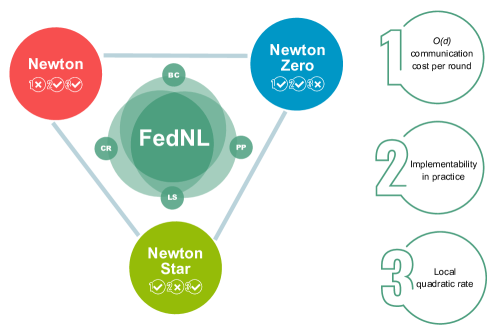
Figure 1: Visualization of the three special Newton-type methods—Newton (N), Newton Star (NS) and Newton Zero (N0)—as the vertices of a triangle capturing a subset of two of these three requirements: 1) $\mathcal{O}(d)$ communication cost per round, 2) implementability in practice, and 3) local quadratic rate. Indeed, each of these three methods satisfies two of these requirements only: N (2+3), NS (1+3) and N0 (1+2). Finally, the proposed FedNL framework with its four extensions to Partial Participation (FedNL-PP), globalization via Line Search (FedNL-LS), globalization via Cubic Regularization (FedNL-CR) and Bidirectional Compression (FedNL-BC) interpolates between these requirements.

4 FedNL with Partial Participation, Globalization and Bidirectional Compression

Here we briefly describe four extensions to FedNL and the key technical contributions. Detailed sections for each extension are deferred to the Appendix.

4.1 Partial Participation (see Section D)

In FedNL-PP (Algorithm 2), the server selects a subset $S^{k}\subseteq[n]$ of $\tau$ devices, uniformly at random, to participate in each iteration. As devices might be inactive for several iterations, the same local gradient and local Hessian used in FedNL does not provide convergence in this case. To guarantee convergence, devices need to compute Hessian corrected local gradients

$$g_{i}^{k}=(\mathbf{H}_{i}^{k}+l_{i}^{k}\mathbf{I})w_{i}^{k}-\nabla f_{i}(w_{i}^{k}),$$

where $w_{i}^{k}$ is the last global model that device $i$ received from the server. This is an innovation which also requires a different analysis.

4.2 Globalization via Line Search (see Section E)

Our first globalization strategy, FedNL-LS (Algorithm 3), which performs significantly better in practice than FedNL-CR (described next), is based on a backtracking line search procedure. The idea is to fix the search direction

$$d^{k}=-\left[\mathbf{H}^{k}\right]_{\mu}^{-1}\nabla f(x^{k})$$

by the server and find the smallest integer $s\geq 0$ which leads to a sufficient decrease in the loss

$$f(x^{k}+\gamma^{s}d^{k})\leq f(x^{k})+c\gamma^{s}\left\langle\nabla f(x^{k}),d^{k}\right\rangle$$

with some parameters $c\in(0,\nicefrac{{1}}{{2}}]$ and $\gamma\in(0,1)$.

4.3 Globalization via Cubic Regularization (see Section F)

Our next globalization strategy, FedNL-CR (Algorithm 4), is to use a cubic regularization term $\frac{L_{*}}{6}\|h\|^{3}$, where $L_{*}$ is the Lipschitz constant for Hessians and $h$ is the direction to the next iterate. However, to get a global upper bound, we had to correct the global Hessian estimate $\mathbf{H}^{k}$ via compression error $l^{k}$. Indeed, since $\nabla^{2}f(x^{k})\preceq\mathbf{H}^{k}+l^{k}\mathbf{I}$, we deduce

$$f(x^{k+1})\leq f(x^{k})+\left\langle\nabla f(x^{k}),h^{k}\right\rangle+\frac{1}{2}\left\langle(\mathbf{H}^{k}+l^{k}\mathbf{I})h^{k},h^{k}\right\rangle+\frac{L_{*}}{6}\|h^{k}\|^{3}$$

for all $k\geq 0$. This leads to theoretical challenges and necessitates a new analysis.

4.4 Bidirectional Compression (see Section G)

Finally, we modify FedNL to allow for an even more severe level of compression that can’t be attained by compressing the Hessians only. This is achieved by compressing the gradients (uplink) and the model (downlink), in a ‘‘smart’’ way. In FedNL-BC (Alg. 5), the server operates its own compressors ${\mathcal{C}}^{k}_{\rm M}$ applied to the model, and uses an additional ‘‘smart’’ model learning technique similar to the proposed Hessian learning technique. Besides, all devices compress their local gradients via a Bernoulli compression scheme, which necessitates the use of another ‘‘smart’’ strategy using Hessian corrected local gradients

$$g_{i}^{k}=\mathbf{H}_{i}^{k}(z^{k}-w^{k})+\nabla f_{i}(w^{k}),$$

where $z^{k}$ is the current learned global model and $w^{k}$ is the last learned global model when local gradients are sent to the server. These changes are substantial and require novel analysis.

5 Experiments

We carry out numerical experiments to study the performance of FedNL, and compare it with various state-of-the-art methods in federated learning. We consider the problem (1) with local loss functions

$$\min\limits_{x\in\mathbb{R}^{d}}\left\{f(x)\;{:=}\;\frac{1}{n}\sum\limits_{i=1}^{n}f_{i}(x)+\frac{\lambda}{2}\|x\|^{2}\right\},\qquad f_{i}(x)=\frac{1}{m}\sum\limits_{j=1}^{m}\log\left(1+\exp(-b_{ij}a_{ij}^{\top}x)\right),$$ (11)

where $\{a_{ij},b_{ij}\}_{j\in[m]}$ are data points at the $i$-th device and $\lambda>0$ is a regularization parameter. The datasets were taken from LibSVM library (Chang and Lin, 2011): a1a, a9a, w7a, w8a, and phishing.

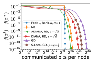
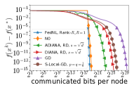
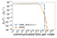
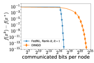
(a) madelon, $\lambda=10^{-3}$	(b) a1a, $\lambda=10^{-4}$	(c) w8a, $\lambda=10^{-3}$	(d) phishing, $\lambda=10^{-4}$

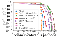
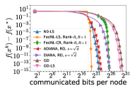
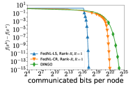
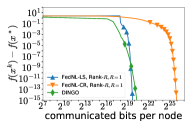
(a) madelon, $\lambda=10^{-3}$	(b) a1a, $\lambda=10^{-4}$	(c) phishing, $\lambda=10^{-3}$	(d) a9a, $\lambda=10^{-4}$

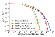
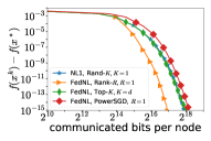
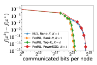
(a) w8a, $\lambda=10^{-3}$	(b) phishing, $\lambda=10^{-3}$	(c) a1a, $\lambda=10^{-4}$	(d) w7a, $\lambda=10^{-4}$

Figure 2: First row: Local comparison of FedNL and N0 with (a), (b) ADIANA, DIANA, GD; with (c), (d) DINGO in terms of communication complexity. Second row: Global comparison of FedNL-LS, N0-LS and FedNL-CR with (a), (b) ADIANA, DIANA, GD, and GD with line search; with (c), (d) DINGO in terms of communication complexity. Third row: Local comparison of FedNL with $3$ types of compression operators and NL1 in terms of communication complexity.

5.1 Parameter setting

In all experiments we use the theoretical parameters for gradient type methods (except those using line search): vanilla gradient descent GD, DIANA (Mishchenko et al., 2019), ADIANA (Li et al., 2020b), and Shifted Local gradient descent, S-Local-GD (Gorbunov et al., 2021b). For DINGO (Crane and Roosta, 2019) we use the authors’ choice: $\theta=10^{-4},\phi=10^{-6},\rho=10^{-4}$. Backtracking line search for DINGO selects the largest stepsize from $\{1,2^{-1},\dots,2^{-10}\}.$ The initialization of $\mathbf{H}^{0}_{i}$ for NL1 (Islamov et al., 2021), FedNL and FedNL-LS is $\nabla^{2}f_{i}(x^{0})$, and for FedNL-CR is $\mathbf{0}$. For FedNL, FedNL-LS, and FedNL-CR we use Rank-$1$ compression operator and stepsize $\alpha=1$. We use two values of the regularization parameter: $\lambda\in\{10^{-3},10^{-4}\}$. In the figures we plot the relation of the optimality gap $f(x^{k})-f(x^{*})$ and the number of communicated bits per node, or the number of communication rounds. The optimal value $f(x^{*})$ is chosen as the function value at the $20$-th iterate of standard Newton’s method.

5.2 Local convergence

In our first experiment we compare FedNL and N0 with gradient type methods: ADIANA with random dithering (ADIANA, RD, $s=\sqrt{d}$), DIANA with random dithering (DIANA, RD, $s=\sqrt{d}$), Shifted Local gradient descent (S-Local-GD, $p=q=\frac{1}{n}$), vanilla gradient descent (GD), and DINGO. According to the results summarized in Figure 2 (first row), we conclude that FedNL outperforms all gradient type methods and DINGO, locally, by many orders in magnitude. We want to note that we include the communication cost of the initialization for FedNL and N0 in order to make a fair comparison (this is why there is a straight line for these methods initially).

5.3 Global convergence

We now compare FedNL-LS, N0-LS, and FedNL-CR with the first-order methods ADIANA and DIANA with random dithering, Shifted Local gradient descent S-Local-GD, gradient descent (GD), and GD with line search (GD-LS). Besides, we compare FedNL-LS and FedNL-CR with DINGO. In this experiment we choose $x^{0}$ far from the solution $x^{*}$, i.e., we test the global convergence behavior; see Figure 2 (second row). We observe that FedNL-LS is more communication efficient than all first-order methods and DINGO. However, FedNL-CR is better than GD and GD-LS only. In these experiments we again include the communication cost of initialization for FedNL-LS and N0-LS.

5.4 Comparison with NL1

Next, we compare FedNL with three type of compression operators: Rank-$R$ ($R=1$), Top-$K$ ($K=d$), and PowerSGD (Vogels et al., 2019) ($R=1$) against NL1 with the Rand-$K$ ($K=1$) compressor. The results, presented in Figure 2 (third row), show that FedNL with Rank-$1$ compressor performs the best.

Appendix

Appendix A Theoretical Comparisons with Related Works

In this part, we compare our results with the most relevant prior works in the literature. We start comparing our work with several recently proposed second order distributed optimization methods to the following criterias: problem structure, assumptions on the loss functions, communication complexity (the number of encoding bits sent from client to server in each communication round), theoretical convergence rate and other aspects of the method (such as local computation and privacy). Table 4 below provides the summary.

Table 4: Theoretical comparison of 7 second order methods (including ours). Advantages are written in green, while limitations are colored in red.

Method	Problem	Assumptions	Comm. Cost per Round	Rate	Comments
GIANT [Wang et al., 2018]	GLM2	LipC1 Hessian, convex $+\,l_{2}$ reg., $\approx$ i.i.d. data	$\mathcal{O}(d)$	Local $\kappa$-dependent linear. Global $\mathcal{O}(\log\nicefrac{{\kappa}}{{\epsilon}})$, quadratics	Big data regime (#data$\,\gg d$)
DINGO [Crane and Roosta, 2019]	GFS3	Moral Smoothness4, $\approx$ strong convexity5	$\mathcal{O}(d)$	Global linear rate. No fast local rate.	Operates full gradients, Hessian-vector products, Hessian pseudo-inverse and vector products.
DAN [Zhang et al., 2020]	GFS	LipC Hessian, strong convexity	$\mathcal{O}(nd^{2})$	Global quadratic rate after $\mathcal{O}(\nicefrac{{L}}{{\mu^{2}}})$ iterations.	Operates full gradients and Hessian matrices.
DAN-LA [Zhang et al., 2020]	GFS	LipC Hessian, LipC gradient, strong convexity	$\mathcal{O}(nd)$	Asymptotic and implicit global superlinear rate.	$\lim_{k\to\infty}\frac{\|x_{k+1}-x^{*}\|}{\|x_{k}-x^{*}\|}=0$ Independent of $\kappa$ ? Better non-asymptotic complexity over linear rate ?
NL [Islamov et al., 2021]	GLM	LipC Hessian, convex $+\,l_{2}$ reg.	$\mathcal{O}(d)$	Local superlinear rate independent of $\kappa$, but dependent on #data. Global linear rate.	reveals local data to server
Quantized Newton [Alimisis et al., 2021]	GFS	LipC Hessian, LipC gradient, strong convexity5	$\widetilde{\mathcal{O}}(d^{2})$	Local (fixed) linear rate. No global rate.	Operates full gradients and Hessian matrices.
FedNL (this work)	GFS	LipC Hessian, strong convexity	$\mathcal{O}(d)$	Local (fixed) linear rate. Local superlinear rate independent of $\kappa$, independent of #data. Global linear rate.	Operates full gradients and Hessian matrices. Supports contractive Hessian compression. Extensions†

• ¹ LipC = Lipschitz Continuous.

• ² GLM = Generalized Linear Model, e.g. $loss_{j}(x;a_{j})=\phi_{j}(a_{j}^{\top}x)+\lambda\|x\|^{2}.$   ³ GFS = General Finite Sum.

• ⁴ Moral Smoothness: $\|\nabla^{2}f(x)\nabla f(x)-\nabla^{2}f(y)\nabla f(y)\|\leq L\|x-y\|$.   ⁵ Applies to local loss functions for all clients.

• ^† Partial Participation, Globalization (via Line Search and Cubic Regularization) and Bidirectional Compression.

As we can see from the table, in contrast to FedNL, the other methods suffer at least one of the following issues:

• Theoretical analysis does not cover general finite sum problems (GIANT and NL).

• Communication cost per client/iteration is high (DAN and Quantized Newton).

• Convergence rate either depends on condition number (GIANT and DINGO) or the number of data points (NL) or is not explicit/clear (DAN-LA).

• Privacy is broken by directly revealing local training data (NL).

We do not compare with algorithms DANE [Shamir et al., 2014] and its accelerated variant AIDE [Reddi et al., 2016] since they are first-order methods. This means that convergence rates depend on the conditioning of the problem and hence are worse than what we prove for FedNL. Moreover, DANE does not work well for heterogeneous datasets - the analysis and experimental evidence of DANE only shows benefits in a sufficiently homogeneous data regime. On the other hand, our concern is the heterogeneous data regime typical to FL. We also omit DiSCO [Zhang and Lin, 2015] from our empirical study because the problem setup is restricted to homogeneous data distribution regime, generalized linear models and convergence rates depend on the conditioning of the problem. Furthermore, the authors of DINGO experimentally showed that DINGO outperforms methods like DiSCO and GIANT, and this is why we focused on comparing to DINGO.

Next, we compare several first and second order methods based on their communication complexity, defined as the total number of bits sent from a client to the server to achieve some prescribed accuracy $\epsilon$. For this purpose, we use sparsification as an example of a compressor in most cases. For all methods supporting sparsification, we have used the sparsification, which reduces the number of communicated floats by the factor of $d$ compared to the non-compressed variant of the method. That is, for gradient based methods DCGD, DIANA and ADIANA, we have used the Rand-1 sparsifier, which compresses $\mathcal{O}(d)$ gradient to $\mathcal{O}(1)$.

To transform the local superlinear convergence rate (9) of FedNL into an iteration complexity, we proceed as follows. Let $r_{k+1}\leq C(1-\rho)^{k}r_{k}$, where $r_{k}=\|x^{k}-x^{*}\|^{2}$, $\rho\in(0,1)$ and $C>0$ is some constant. Note that if $k\geq\frac{2}{\rho}\log\frac{1}{C}$, then $(1-\rho)^{\nicefrac{{k}}{{2}}}C\leq 1$. Hence, after $\mathcal{O}(\frac{1}{\rho})$ iteration we have $r_{k+1}\leq(1-\rho)^{\nicefrac{{k}}{{2}}}r_{k}$. Unraveling the recursion we get

$$r_{k}\leq(1-\rho)^{\frac{k-1}{2}}(1-\rho)^{\frac{k-2}{2}}\dots(1-\rho)^{\frac{1}{2}}r_{0}=(1-\rho)^{\frac{k(k-1)}{2}}r_{0}.$$

Therefore, FedNL needs $\mathcal{O}\left(\sqrt{\frac{1}{\rho}\log\frac{1}{\epsilon}}\right)$ number of iterations to achieve $\epsilon$-accuracy. For FedNL, we used step-size $\alpha=1$ (see Assumption 3.4(ii) and also (5)) and matrix sparsification described in Appendix B.3.3, which compresses $\mathcal{O}(d^{2})$ Hessian down to $\mathcal{O}(d)$ (i.e., $\delta=\frac{1}{d}$). With this choice we get $\frac{1}{\rho}=\mathcal{O}(d)$ and the iteration of FedNL becomes $\mathcal{O}\left(\sqrt{d\log\frac{1}{\epsilon}}\right)$. For Newton Learn (NL), $\frac{1}{\rho}=\mathcal{O}(\#\text{data})$, where $\#\text{data}$ is the number of data points in each device. DAN and Quantized Newton use their own bespoke ways of compressing communication. Table 5 provides the details, from which we make the following observations:

Table 5: Theoretical comparison of 3 gradient-based and 5 second-order methods. The last column (communication complexity) is the product of the previous two columns and is the key quantity to be compared.

Method	# Communication Rounds	Comm. Cost per Round	Communication Complexity
Gradient Descent1	$\mathcal{O}(\kappa\log\frac{1}{\epsilon})$	$\mathcal{O}(d)$	$\mathcal{O}(d\kappa\log\frac{1}{\epsilon})$
DCGD1 Khirirat et al. [2018]	$\mathcal{O}\left(\frac{d\sigma^{*}}{n\mu^{2}}\frac{1}{\epsilon}\log\frac{1}{\epsilon}\right)$	$\mathcal{O}(1)$	$\mathcal{O}\left(\frac{d\sigma^{*}}{n\mu^{2}}\frac{1}{\epsilon}\log\frac{1}{\epsilon}\right)$
DIANA1 Mishchenko et al. [2019]	$\mathcal{O}\left(\left(d+\kappa+\kappa\frac{d}{n}\right)\log\frac{1}{\epsilon}\right)$	$\mathcal{O}(1)$	$\mathcal{O}\left(\left(d+\kappa+\kappa\frac{d}{n}\right)\log\frac{1}{\epsilon}\right)$
ADIANA1 Li et al. [2020b]	$\mathcal{O}\left(\left(d+\sqrt{\kappa}+\sqrt{\left(\frac{d}{n}+\sqrt{\frac{d}{n}}\right)d\kappa}\right)\log\frac{1}{\epsilon}\right)$	$\mathcal{O}(1)$	$\mathcal{O}\left(\left(d+\sqrt{\kappa}+\sqrt{\left(\frac{d}{n}+\sqrt{\frac{d}{n}}\right)d\kappa}\right)\log\frac{1}{\epsilon}\right)$
Newton	$\mathcal{O}(\log\log\frac{1}{\epsilon})$	$\mathcal{O}(d^{2})$	$\mathcal{O}(d^{2}\log\log\frac{1}{\epsilon})$
DAN1 Zhang et al. [2020]	$\mathcal{O}\left(\frac{L_{*}}{\mu^{2}}+\log\log\frac{1}{\epsilon}\right)$	$\mathcal{O}(d^{2})$	$\mathcal{O}\left(d^{2}\left(\frac{L_{*}}{\mu^{2}}+\log\log\frac{1}{\epsilon}\right)\right)$
Quantized Newton [Alimisis et al., 2021]	$\mathcal{O}(\log\frac{1}{\epsilon})$	$\widetilde{\mathcal{O}}(d^{2})$	$\widetilde{\mathcal{O}}(d^{2}\log\frac{1}{\epsilon})$
NL [Islamov et al., 2021]	$\mathcal{O}\left(\sqrt{\#\text{data}}\sqrt{\log\frac{1}{\epsilon}}\right)$	$\mathcal{O}(d)$	$\mathcal{O}\left(d\sqrt{\#\text{data}}\sqrt{\log\frac{1}{\epsilon}}\right)$
FedNL (this work; (7))	$\mathcal{O}\left(\log\frac{1}{\epsilon}\right)$	$\mathcal{O}(d)$	$\mathcal{O}\left(d\log\frac{1}{\epsilon}\right)$
FedNL (this work; (9))	$\mathcal{O}\left(\sqrt{d}\sqrt{\log\frac{1}{\epsilon}}\right)$	$\mathcal{O}(d)$	$\mathcal{O}\left(d\sqrt{d}\sqrt{\log\frac{1}{\epsilon}}\right)$

• ¹ These methods have global rates.  ² DCGD, DIANA and ADIANA are first order methods.

• ³ Newton, DAN, Quantized Newton, NL and FedNL are second order methods.

• ⁴ $\kappa$ is the condition number: $\kappa=\frac{L}{\mu}$ where $L$ is a smoothness constant and $\mu$ is the strong convexity constant.

• FedNL achieves better communication complexity than Newton whenever $d>\frac{\log\frac{1}{\epsilon}}{\left(\log\log\frac{1}{\epsilon}\right)^{2}}$. For example, if we set $\epsilon=10^{-10}$, then this requirement means $d>10$, and hence is not restrictive. So, virtually in all situations of practical interest, FedNL is better than Newton. The improvement is more pronounced with larger $d$, and is approximately of the size $\mathcal{O}(\sqrt{d})$. So, for $d=10^{6}$, for example, FedNL finds the solution using approximately 1000 times less communicated bits than Newton.

• FedNL achieves better communication complexity than Gradient Descent whenever $\kappa>\frac{\sqrt{d}}{\sqrt{\log\frac{1}{\epsilon}}}$. So, FedNL is better when the condition number $\kappa$ is large enough. This is expected, since FedNL complexity does not depend on the condition number. The advantage of FedNL grows if $d$ or $\epsilon$ are smaller.

• ADIANA is known to have the state of the art complexity (in the strongly convex regime) among all first order method, and hence we do not need to compare FedNL to DCGD and DIANA, which are both inferior to ADIANA. It is clear that FedNL can beat ADIANA as well since the complexity of ADIANA depends on $\kappa$. So, for large enough $\kappa$, FedNL is better than ADIANA. For example, a simple sufficient condition for this to happen is to require $\kappa>d^{3}$ (this can be refined, but the expression will become uglier). Likewise, FedNL has square root dependence on $\log\frac{1}{\epsilon}$, and hence it becomes better than ADIANA if $\epsilon$ is sufficiently small (and other terms are kept constant).

• Neither Quantized Newton nor DAN improve on Newton in communication complexity (but may be better in practice). We already explained that FedNL improves on Newton.

• We do not include GIANT in the table since GIANT does not work in the heterogeneous data regime, which is critical to FL and our paper. We do not include DINGO in the table since its rate depends on various iterate-dependent assumptions which make the analysis convoluted. It is not clear that such assumptions can actually be satisfied. Their rates are not explicit - it is not possible to compare to them.

It worths noting that our work is not just about communication complexity. In fact, our contributions go far beyond this, and we make it clear in the paper. Our work is the first serious attempt to make second order methods applicable to federated learning in the sense that we address many issues which previously made second order methods inapplicable to FL. We support compression of matrices, rudimentary privacy protection (by not revealing data), partial participation, compression of (Hessian corrected) gradients, compression of model (at the master), arbitrary (strongly convex) finite sum problems rather than generalized linear models only, arbitrary contractive compressors, two globalization strategies and more. The best way to judge our contribution to the literature is via comparison to the NewtonLearn work of Islamov et al. [2021] as their work is the closest work to ours and was the SOTA second order method supporting communication compression before our work. We have made a very detailed comparison to their work, including tables.

Appendix B Extra Experiments

We carry out numerical experiments to study the performance of FedNL, and compare it with various state-of-the-art methods in federated learning. We consider the following problem

$$\min\limits_{x\in\mathbb{R}^{d}}\left\{\frac{1}{n}\sum\limits_{i=1}^{n}f_{i}(x)+\frac{\lambda}{2}\|x\|^{2}\right\},\quad f_{i}(x)=\frac{1}{m}\sum_{j=1}^{m}\log\left(1+\exp(-b_{ij}a_{ij}^{\top}x)\right),$$ (12)

where $\{a_{ij},b_{ij}\}_{j\in[m]}$ are data points at the $i$-th device.

B.1 Data sets

The datasets were taken from LibSVM library [Chang and Lin, 2011]: a1a, a9a, w7a, w8a, phishing. We partitioned each data set across several nodes to capture a variety of scenarios. See Table 6 for more detailed description of data sets settings.

Table 6: Data sets used in the experiments with the number of worker nodes $n$ used in each case.

Data set	# workers $n$	# data points ($=nm$)	# features $d$
a1a	$16$	$1600$	$123$
a9a	$80$	$32560$	$123$
w7a	$50$	$24600$	$300$
w8a	$142$	$49700$	$300$
phishing	$100$	$110$	$68$
madelon	$10$	$2000$	$500$

B.2 Parameters setting

In all experiments we use theoretical parameters for gradient type methods (except those with line search procedure): vanilla gradient descent, DIANA [Mishchenko et al., 2019], ADIANA [Li et al., 2020b], and Shifted Local gradient descent [Gorbunov et al., 2021b]. The constants for DINGO [Crane and Roosta, 2019] are set as the authors did: $\theta=10^{-4},\phi=10^{-6},\rho=10^{-4}$. Backtracking line search for DINGO selects the largest stepsize from $\{1,2^{-1},\dots,2^{-10}\}.$ The initialization of $\mathbf{H}^{0}_{i}$ for NL1 [Islamov et al., 2021], FedNL, FedNL-LS, and FedNL-PP is $\nabla^{2}f_{i}(x^{0})$, and for FedNL-CR is $\mathbf{0}$.

We conduct experiments for two values of regularization parameter $\lambda\in\{10^{-3},10^{-4}\}$. In the figures we plot the relation of the optimality gap $f(x^{k})-f(x^{*})$ and the number of communicated bits per node or the number of communication rounds. The optimal value $f(x^{*})$ is chosen as the function value at the $20$-th iterate of standard Newton’s method.

B.3 Compression operators

Here we describe four compression operators that are used in our experiments.

B.3.1 Random dithering for vectors

For first order methods ADIANA and DIANA we use random dithering operator [Alistarh et al., 2017, Horváth et al., 2019]. This compressor with $s$ levels is defined via the following formula

$${\mathcal{C}}(x)\;{:=}\;\text{sign}(x)\cdot\|x\|_{q}\cdot\frac{\xi_{s}}{s},$$ (13)

where $\|x\|_{q}\;{:=}\;\left(\sum_{i}|x_{i}|^{q}\right)^{1/q}$ and $\xi_{s}\in\mathbb{R}^{d}$ is a random vector with $i$-th element defind as follows

$$(\xi_{s})_{i}=\begin{cases}l+1&\text{with probability }\frac{|x_{i}|}{\|x\|_{q}}s-l,\\ l&\text{otherwise}.\end{cases}$$ (14)

Here $s\in\mathbb{N}_{+}$ denotes the levels of rounding, and $l$ satisfies $\frac{|x_{i}|}{\|x\|_{q}}\in\left[\frac{l}{s},\frac{l+1}{s}\right]$. According to [Horváth et al., 2019], this compressor has the variance parameter $\omega\leq 2+\frac{d^{1/2}+d^{1/q}}{s}.$ However, for standard euclidean norm ($q=2$) one can improve the bound by $\omega\leq\min\left\{\frac{d}{s^{2}},\frac{\sqrt{d}}{s}\right\}$ [Alistarh et al., 2017].

B.3.2 Rank-$R$ compression operator for matrices

Our theory supports contractive compression operators; see Definition 3.3. In the experiments for FedNL we use Rank-$R$ compression operator. Let $\mathbf{X}\in\mathbb{R}^{d\times d}$ and $\mathbf{U}\Sigma\mathbf{V}^{\top}$ be the singular value decomposition of $\mathbf{X}$:

$$\mathbf{X}=\sum\limits_{i=1}^{d}\sigma_{i}u_{i}v_{i}^{\top},$$ (15)

where the singular values $\sigma_{i}$ are sorted in non-increasing order: $\sigma_{1}\geq\sigma_{2}\geq\cdots\geq\sigma_{d}$. Then, the Rank-$R$ compressor, for $R\leq d$, is defined by

$${\mathcal{C}}(\mathbf{X})\;{:=}\;\sum\limits_{i=1}^{R}\sigma_{i}u_{i}v_{i}^{\top}.$$ (16)

Note that

$$\|\mathbf{X}\|^{2}_{\rm F}\overset{\eqref{eq:b97gs_9098fd}}{=}\left\|\sum\limits_{i=1}^{d}\sigma_{i}u_{i}v_{i}^{\top}\right\|^{2}_{\rm F}=\sum_{i=1}^{d}\sigma_{i}^{2}$$

and

$$\|{\mathcal{C}}(\mathbf{X})-\mathbf{X}\|^{2}_{\rm F}\overset{\eqref{eq:b97gs_9098fd}+\eqref{eq:n988fdgfd}}{=}\left\|\sum\limits_{i=R+1}^{d}\sigma_{i}u_{i}v_{i}^{\top}\right\|^{2}_{\rm F}=\sum_{i=R+1}^{d}\sigma_{i}^{2}.$$

Since $\frac{1}{d-R}\sum_{i=R+1}^{d}\sigma_{i}^{2}\leq\frac{1}{d}\sum_{i=1}^{d}\sigma_{i}^{2}$, we have

$$\|{\mathcal{C}}(\mathbf{X})-\mathbf{X}\|^{2}_{\rm F}\leq\frac{d-R}{d}\|\mathbf{X}\|^{2}_{\rm F}=\left(1-\frac{R}{d}\right)\|\mathbf{X}\|^{2}_{\rm F},$$

and hence the Rank-$R$ compression operator belongs to $\mathbb{C}(\delta)$ with $\delta=\frac{R}{d}.$ In case when $\mathbf{X}\in\mathbb{S}^{d}$, we have $u_{i}=v_{i}$ for all $i\in[d]$, and Rank-$R$ compressor on matrix $\mathbf{X}$ transforms to $\sum_{i=1}^{R}\sigma_{i}u_{i}u_{i}^{\top}$, i.e., the output of Rank-$R$ compressor is automatically a symmetric matrix, too.

B.3.3 Top-$K$ compression operator for matrices

Another example of contractive compression operators is Top-$K$ compressor for matrices. For arbitrary matrix $\mathbf{X}\in\mathbb{R}^{d\times d}$ let sort its entires in non-increasing order by magnitude, i.e., $X_{i_{k},j_{k}}$ is the $k$-th maximal element of $\mathbf{X}$ by magnitude. Let’s $\{\mathbf{E}_{ij}\}_{i,j=1}^{d}$ me matrices for which

$$\left(\mathbf{E}_{ij}\right)_{ps}\;{:=}\;\begin{cases}1,&\text{if }(p,s)=(i,j),\\ 0,&\text{otherwise.}\end{cases}$$ (17)

Then, the Top-$K$ compression operator can be defined via

$${\mathcal{C}}(\mathbf{X})\;{:=}\;\sum\limits_{k=1}^{K}X_{i_{k},j_{k}}E_{i_{k},j_{k}}.$$ (18)

This compression operator belongs to $\mathbb{C}(\delta)$ with $\delta=\frac{K}{d^{2}}$. If we need to keep the output of Top-$K$ on symmetric matrix $\mathbf{X}$ to be symmetric matrix too, then we apply Top-$K$ compressor only on lower triangular part of $\mathbf{X}$.

B.3.4 Rand-$K$ compression operator for matrices

Our theory also supports unbiased compression operators; see Definition 3.2. One of the examples is Rand-$K$. For arbitrary matrix $\mathbf{X}\in\mathbb{R}^{d\times d}$ we choose a set $\mathcal{S}_{K}$ of indexes $(i,j)$ of cardinality $K$ uniformly at random. Then Rand-$K$ compressor can be defined via

$${\mathcal{C}}\left(\mathbf{X}\right)_{ij}\;{:=}\;\begin{cases}\frac{d^{2}}{K}X_{ij}&\text{if }(i,j)\in\mathcal{S}_{K},\\ 0&\text{otherwise}.\end{cases}$$ (19)

This compression operator belongs to $\mathbb{B}(\omega)$ with $\omega=\frac{d^{2}}{K}-1$. If we need to make the output of this compressor to be symmetric matrix, then we apply this compressor only on lower triangular part of the input.

B.4 Projection onto the cone of positive definite matrices

If one uses FedNL with Option $1$, then we need to project onto the cone of symmetric and positive definite matrices with constant $\mu$:

$$\{\mathbf{M}\in\mathbb{R}^{d\times d}:\mathbf{M}^{\top}=\mathbf{M},\;\mathbf{M}\succeq\mu\mathbf{I}\}.$$

The projection of symmetric matrix $\mathbf{X}$ onto the cone of positive semidefinite matrices can by computed via

$$\left[\mathbf{X}\right]_{0}\;{:=}\;\sum\limits_{i=1}^{d}\max\{\lambda_{i},0\}u_{i}u_{i}^{\top},$$ (20)

where $\sum_{i}\lambda_{i}u_{i}u_{i}^{\top}$ is an eigenvalue decomposition of $\mathbf{X}$. Using the projection onto the cone of positive semidefinite matrices we can define the projection onto the cone of positive definite matrices with constant $\mu$ via

$$\left[\mathbf{X}\right]_{\mu}\;{:=}\;\left[\mathbf{X}-\mu\mathbf{I}\right]_{0}+\mu\mathbf{I}.$$ (21)

B.5 The effect of compression

First, we investigate how the level of compression influences the performance of FedNL; see Figure 3. Here we study the performance for three types of compression operators: Rank-$R$, Top-$K$, and PowerSGD of rank $R$. According to numerical experiments, the smaller parameter is, the better performance of FedNL is. This statement is true for all three types of compressors.

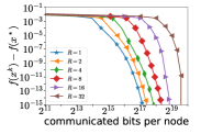
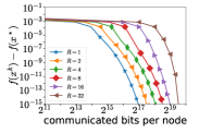
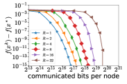
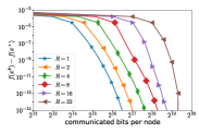
a1a, $\lambda=10^{-3}$	a1a, $\lambda=10^{-4}$	a9a, $\lambda=10^{-3}$	a9a, $\lambda=10^{-4}$
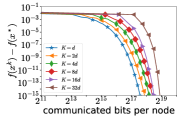
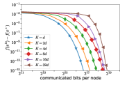
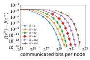
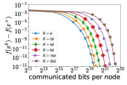
phishing, $\lambda=10^{-3}$	phishing, $\lambda=10^{-4}$	w7a, $\lambda=10^{-3}$	w8a, $\lambda=10^{-3}$
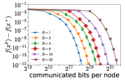
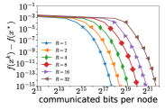
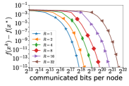
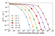
a1a, $\lambda=10^{-3}$	a1a, $\lambda=10^{-4}$	a9a, $\lambda=10^{-3}$	a9a, $\lambda=10^{-4}$

Figure 3: The performance of FedNL with different types of compression operators: Rank-$R$ (first row); Top-$K$ (second row); PowerSGD of rank $R$ (third row) for several values of $R$ and $K$ in terms of communication complexity.

B.6 Comparison of Options $1$ and $2$

In our next experiment we investigate which Option ($1$ or $2$) for FedNL with Rank-$R$ and stepsize $\alpha=1$ compressor demonstrates better results in terms of communication compexity. According to the results in Figure 4, we see that FedNL with projection (Option $1$) is more communication effective than that with Option $2$. However, Option $1$ requires more computing resources.

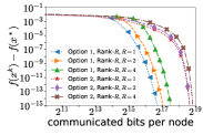
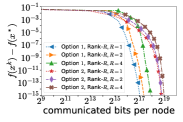
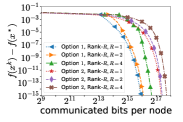
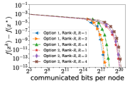
a1a, $\lambda=10^{-3}$	a9a, $\lambda=10^{-3}$	phishing, $\lambda=10^{-4}$	w7a, $\lambda=10^{-4}$

Figure 4: The performance of FedNL with Options $1$ and $2$ in terms of communication complexity.

B.7 Comparison of different compression operators

Next, we study which compression operator is better in terms of communication complexity. Based on the results in Figure 5, we can conclude that Rank-$R$ is the best compression operator; Top-$K$ and PowerSGD compressors can beat each other in different cases.

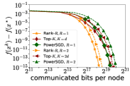
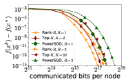
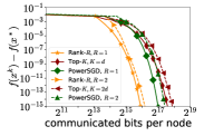
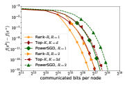
w8a, $\lambda=10^{-3}$	a1a, $\lambda=10^{-4}$	phishing, $\lambda=10^{-3}$	a9a, $\lambda=10^{-4}$

Figure 5: Comparison of the performance of FedNL with different compression operators in terms of communication complexity.

B.8 Comparison of different update rules for Hessians

On the following step we compare FedNL with three update rules for Hessians in order to find the best one. They are biased Top-$K$ compression operator with stepsize $\alpha=1$ (Option $1$); biased Top-$K$ compression operator with stepsize $\alpha=1-\sqrt{1-\delta}$; unbiased Rand-$K$ compression operator with stepsize $\alpha=\frac{1}{\omega+1}$. The results of this experiment are presented in Figure 6. Based on them, we can make a conclusion that FedNL with Top-$K$ compressor and stepsize $\alpha=1$ demonstrates the best performance. FedNL with Rand-$K$ compressor and stepsize $\alpha=\frac{1}{\omega+1}$ performs a little bit better than that with Top-$K$ compressor and stepsize $\alpha=1-\sqrt{1-\delta}$. As a consequence, we will use biased compression operator with stepsize $\alpha=1$ for FedNL in further experiments.

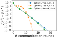
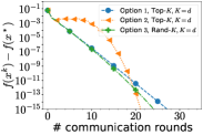
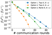
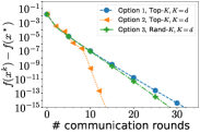
(a) a1a, $\lambda=10^{-3}$	(b) a9a, $\lambda=10^{-3}$	(c) phishing, $\lambda=10^{-3}$	(d) w7a, $\lambda=10^{-3}$

Figure 6: Comparison of FedNL with three update rules: Top-$K,\alpha=1-\sqrt{1-\delta}$ (Option $1$); Top-$K,\alpha=1$ (Option $2$); Rand-$K,\alpha=\frac{1}{\omega+1}$ (Option $3$) in terms of iteration complexity.

B.9 Bidirectional compression

Now we study how the performance of FedNL-BC (with Option $1$ and stepsize $\alpha=1$) is affected by the level of compression in Figure 7. Here we use Top-$K$ compressor for Hessians and models, and broadcast gradients with probability $p$. In order to make the results more interpretable, we set $K$ to be $pd$, then we carry out experiments for several values of $p$. We clearly see that deep compression ($p=0.5;0.6$) influences negatively the performance of FedNL-BC. However, small compression ($p=0.9$) can be beneficial in some cases (see Figure 7: (b), (d)), but this is not the case for Figure 7: (a), (c), where the best performance is demonstrated by FedNL-BC with $p=1$. We can conclude that only weak compression (the value of $p$ is close to $1$) can improve the performance of FedNL-BC, but the improvement is relatively small.

We also compare FedNL-BC (compression was described above, Option $2$ was used in the experiments) with DORE method [Liu et al., 2020]. This method applies bi-directional compression on gradients (uplink compression) and models (downlink compression). All constants for this method were chosen according theoretical results in the paper. We use random dithering compressor in both directions ($s=\sqrt{d}$). Based on the numerical experiments in Figure 8, we can conclude that FedNL-BC is much more communication efficient method than DORE by many orders in magnitude.

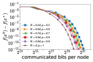
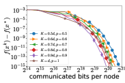
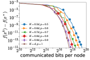
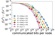
(a) w7a, $\lambda=10^{-3}$	(b) w8a, $\lambda=10^{-3}$	(c) a1a, $\lambda=10^{-4}$	(d) a9a, $\lambda=10^{-4}$

Figure 7: The performance of FedNL-BC with Top-$K$ applied to Hessians and models ($K=pd$), and broadcasting gradients with probability $p$ for several values of $p$ in terms of communication complexity.

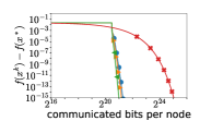
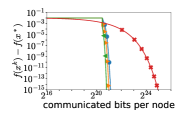
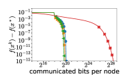
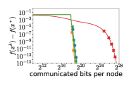
(a) w7a, $\lambda=10^{-3}$	(b) w8a, $\lambda=10^{-3}$	(c) a1a, $\lambda=10^{-4}$	(d) a9a, $\lambda=10^{-4}$

Figure 8: Comparison of FedNL-BC with Top-$K$ applied to Hessians and models ($K=pd$), and broadcasting gradients with probability $p$ and DORE in terms of communication complexity.

B.10 The performance of FedNL-PP

Now we deploy our FedNL-PP method in order to study how the performance is inlfuenced by the value of active nodes $\tau$. We use FedNL-PP with Rank-$1$ compression operator, and run the method for several values of $\tau$; see Figure 9. As we can see, the smaller value of $\tau$ is, the worse performance of FedNL-PP is, as it expected.

Now we compare FedNL-PP with Artemis [Philippenko and Dieuleveut, 2021] which supports partial participation too. We use random sparsification compressor ($s=\sqrt{d}$) in uplink direction, and the server broadcasts descent direction to each node without compression. All contstants of the method were chosen according theory from the paper. Each node $i$ computes full local gradient $\nabla f_{i}(x^{k})$. We conduct experiments for several number of active nodes: $\tau\in\{0.2n,0.4n,0.8n\}$, then we calculate the total number of transmitted bits received by the server from all active nodes. All results are presented in Figure 10. We clearly see that FedNL-PP outperforms Artemis by several orders in magnitude in terms of communication complexity.

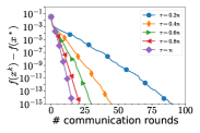
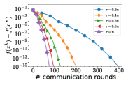
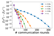
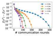
(a) phishing, $\lambda=10^{-3}$	(b) w8a, $\lambda=10^{-3}$	(c) w7a, $\lambda=10^{-4}$	(d) a9a, $\lambda=10^{-4}$

Figure 9: The performance of FedNL-PP with Rank-$1$ compressor in terms of iteration complexity.

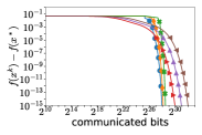
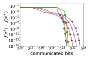
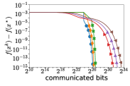
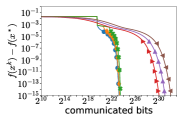
(a) w8a, $\lambda=10^{-3}$	(b) phishing, $\lambda=10^{-3}$	(c) w7a, $\lambda=10^{-4}$	(d) a1a, $\lambda=10^{-4}$

Figure 10: Comparison of FedNL-PP with Artemis in terms of communication complexity for several values of active nodes $\tau$.

B.11 Comparison with NL1

In our next experiment we compare FedNL with three types of compression operators (Rank-$R$, Top-$K$, PowerSGD) and NL1. As we can see in Figure 11, FedNL with Rank-$1$ are more communication efficient method in all cases. FedNL with Top-$d$ and PowerSGD of rank $1$ compressors performs better or the same as NL1 in almost all cases, except Figure 11: (c), where FedNL with PowerSGD demonstrates a little bit worse results than NL1. Based on these experiments, we can conclude that new compression mechanism for Hessians is more effective than that was introduced in [Islamov et al., 2021].

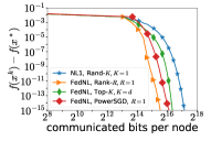
(a) w8a, $\lambda=10^{-3}$	(b) phishing, $\lambda=10^{-3}$	(c) a1a, $\lambda=10^{-4}$	(d) w7a, $\lambda=10^{-4}$

Figure 11: Comparison of FedNL with three types of compression and NL1 in terms of communication complexity.

B.12 Local comparison

Now we compare FedNL (Rank-$1$ compressor, $\alpha=1$) and N0 with first order methods: ADIANA with random dithering (ADIANA, RD, $s=\sqrt{d}$), DIANA with random dithering (DIANA, RD, $s=\sqrt{d}$), Shifted Local gradient descent (S-Local-GD, $p=q=\frac{1}{n}$), and vanilla gradient descent (GD). Here we set $x^{0}$ close to the solution $x^{*}$ in order to highlight fast local rates of FedNL and N0 independent of the condition number. Moreover, we compare FedNL (Rank-$1$ compressor, $\alpha=1$) against DINGO. In order to make fair comparison we calculate transmitted bits in both directions, since DINGO requires several expensive communication round per one iteration of the algorithm. All results are presented in Figure 12. We clearly see that FedNL and N0 are more communication effective methods than gradient type ones. In some cases the difference is large; see Figure 12: (a), (d). In addition FedNL is more effective than DINGO in terms of communication complexity.

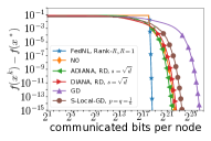
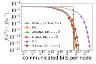
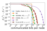
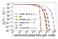
(a) a1a, $\lambda=10^{-3}$	(b) w8a, $\lambda=10^{-3}$	(c) w7a, $\lambda=10^{-4}$	(d) phishing, $\lambda=10^{-4}$
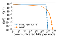
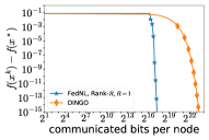
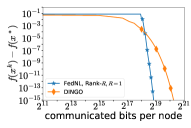
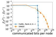
(a) a1a, $\lambda=10^{-3}$	(b) phishing, $\lambda=10^{-3}$	(c) a9a, $\lambda=10^{-4}$	(d) w7a, $\lambda=10^{-4}$

Figure 12: First row: Local comparison of FedNL and N0 with ADIANA, DIANA, S-Local-GD, and GD in terms of communication complexity. Second row: Local comparison of FedNL with DINGO in terms of communication complexity.

B.13 Global compersion

In our next test we compare FedNL-LS (Rank-$1$ compressor, $\alpha=1$), N0-LS, and FedNL-CR (Rank-$1$ compressor, $\alpha=1$) with gradient type methods such as ADIANA with random dithering (ADIANA, RD, $s=\sqrt{d}$), DIANA with random dithering (DIANA, RD, $s=\sqrt{d}$), Shifted Local gradient descent (S-Local-GD, $p=q=\frac{1}{n}$), vanilla gradient descent (GD), and gradient descent with line search (GD-LS). Besides, we compare FedNL-LS (Rank-$1$ compressor, $\alpha=1$) and FedNL-CR (Rank-$1$ compressor, $\alpha=1$) with DINGO. Since DINGO requires several expensive communication round per iteration, we calculate transmitted bits in both directions to make fair comparison. According to numerical experiments, we can conclude that FedNL-LS and N0-LS are more communication effective methods than gradient type ones. In some cases (see Figure 13: (c), (d)) FedNL-CR performs better or the same as DIANA.

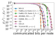
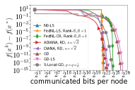
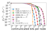
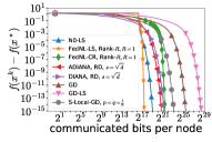
(a) a9a, $\lambda=10^{-3}$	(b) w7a, $\lambda=10^{-3}$	(c) a1a, $\lambda=10^{-4}$	(d) phishing, $\lambda=10^{-4}$
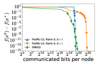
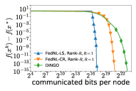
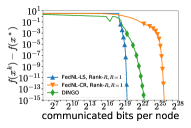
(a) w7a, $\lambda=10^{-3}$	(b) phishing, $\lambda=10^{-3}$	(c) a9a, $\lambda=10^{-4}$	(d) a1a, $\lambda=10^{-4}$

Figure 13: First row: Global comparison of FedNL-LS, N0-LS, and FedNL-CR with ADIANA, DIANA, S-Local-GD, GD, and GD-LS in terms of communication complexity. Second row: Global comparison of FedNL-LS and FedNL-CR with DINGO in terms of communication complexity.

B.14 Effect of statistical heterogeneity

In this set of experiments we investigate the performance of FedNL under different level of heterogeneity of data. We generate synthethic data via rules as [Li et al., 2018] did. We set number of nodes $n=30$, the size of local data $m=200$, the dimension of the problem $d=100$, and regularization parameter $\lambda=10^{-3}$.

The generation rules for non-IID synthetic data have two positive parameteres $\alpha,\beta$. For each node $i\in[n]$ let $B_{i}\sim\mathcal{N}(0,\beta)$. We use diagonal covariance matrix $\Sigma$ with $\Sigma_{j,j}=j^{-1.2}$, and mean vector $v_{i}$, each element of which is generated from $\mathcal{N}(B_{i},1)$ in order to get feature vector $a_{ij}\in\mathbb{R}^{d}$ from $\mathcal{N}(v_{i},\Sigma)$. Let $u_{i}\sim\mathcal{N}(0,\alpha)$, $c_{i}\sim\mathcal{N}(u_{i},1)$, then we generate vector $w_{i}\in\mathbb{R}^{d}$ each entire of which is sampled from $\mathcal{N}(u_{i},1)$. Let $p_{ij}=\sigma\left(w_{i}^{\top}a_{ij}+c_{i}\right)$, where $\sigma(\cdot)$ is a sigmoid function. Finally the label $b_{ij}$ is equal to $-1$ with probability $p_{ij}$, and is equal to $+1$ with probability $1-p_{ij}$. We denote the data which is generated following the rules above as Synthetic $(\alpha,\beta)$.

In addition, we generate IID data where $w\sim\mathcal{N}(0,1)$ and $c\sim\mathcal{N}(0,1)$ are sampled only once and used for each node $i$. Feature vectors $a_{ij}$ is generated from $\mathcal{N}(v_{i},\Sigma)$, where each element of $v_{i}$ is equal to $B_{i}\sim\mathcal{N}(0,\beta)$. The label $b_{ij}$ is equal to $-1$ with probability $p_{ij}=\sigma(w^{\top}a_{ij}+c)$, and $+1$ otherwise. We denote such data as IID.

Using generated synthetic datasets we compare local performance of FedNL (Rank-$1$ compressor, $\alpha=1$, Option $2$), ADIANA with random dithering (ADIANA, RD, $s=\sqrt{d}$), DIANA with random dithering (DIANA, RD, $s=\sqrt{d}$), Shifted Local gradient descent (S-Local-GD, $p=q=\frac{1}{n}$), and vanilla gradient descent (GD) in terms of communication complexit; see Figure 14 (first row). Besides, we compare FedNL and DINGO; see Figure 14 (second row). According to the results, we see that the difference between FedNL and gradient type methods is getting larger, when the local data is becoming more heterogeneous; FedNL outperforms other methods by several orders in magnitude. FedNL is more stable varying data heterogeneity than DINGO. The difference between these two methods on IID data is small; when data is becoming more heterogeneous, the difference is increasing dramatically.

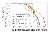
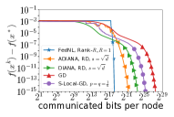
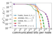
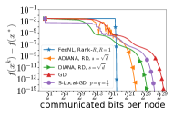
(a) IID	(b) Synthetic ($0.5,0.5$)	(c) Synthetic ($0.75,0.75$)	(d) Syntethic ($1,1$)
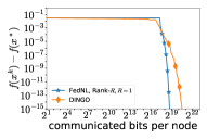
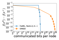
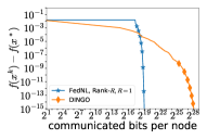
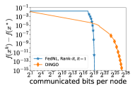
(a) IID	(b) Synthetic ($0.5,0.5$)	(c) Synthetic ($0.75,0.75$)	(d) Syntethic ($1,1$)

Figure 14: First row: Local comparison of FedNL, with ADIANA, DIANA, S-Local-GD, and GD in terms of communication complexity. Second row: Local comparison of FedNL with DINGO in terms of communication complexity.

Appendix C Proofs of Results from Section 3

C.1 Auxiliary lemma

Denote by $\mathbb{E}_{k}\left[\cdot\right]$ the conditional expectation given $k^{th}$ iterate $x^{k}$. We first develop a lemma to handle different cases of compressors for $\mathbb{E}_{k}\|\mathbf{H}_{i}^{k}+\alpha{\mathcal{C}}_{i}^{k}(\nabla^{2}f_{i}(y)-\mathbf{H}_{i}^{k})-\nabla^{2}f_{i}(z)\|^{2}_{\rm F}$, where $\mathbb{E}_{k}[y]=y$ and $\mathbb{E}_{k}[z]=z$.

Lemma C.1.

For any $y$, $z\in\mathbb{R}^{d}$ such that $\mathbb{E}_{k}[y]=y$ and $\mathbb{E}_{k}[z]=z$, we have the following results in different cases.

(i) If ${\mathcal{C}}_{i}^{k}\in\mathbb{B}(\omega)$ and $\alpha\leq\frac{1}{\omega+1}$, then

$$\mathbb{E}_{k}\left[\|\mathbf{H}_{i}^{k}+\alpha{\mathcal{C}}_{i}^{k}(\nabla^{2}f_{i}(y)-\mathbf{H}_{i}^{k})-\nabla^{2}f_{i}(z)\|^{2}_{\rm F}\right]\leq(1-\alpha)\|\mathbf{H}_{i}^{k}-\nabla^{2}f_{i}(z)\|_{\rm F}^{2}+\alpha L_{\rm F}^{2}\|y-z\|^{2}.$$

(ii) If ${\mathcal{C}}_{i}^{k}\in\mathbb{C}(\delta)$ and $\alpha=1-\sqrt{1-\delta}$, then

$$\mathbb{E}_{k}\left[\|\mathbf{H}_{i}^{k}+\alpha{\mathcal{C}}_{i}^{k}(\nabla^{2}f_{i}(y)-\mathbf{H}_{i}^{k})-\nabla^{2}f_{i}(z)\|^{2}_{\rm F}\right]\leq(1-\alpha^{2})\left\|\mathbf{H}_{i}^{k}-\nabla^{2}f_{i}(z)\right\|^{2}_{\rm F}+\alpha L_{\rm F}^{2}\|y-z\|^{2}.$$

(iii) If ${\mathcal{C}}_{i}^{k}\in\mathbb{C}(\delta)$ and $\alpha=1$, then

$$\mathbb{E}_{k}\left[\|\mathbf{H}_{i}^{k}+\alpha{\mathcal{C}}_{i}^{k}(\nabla^{2}f_{i}(y)-\mathbf{H}_{i}^{k})-\nabla^{2}f_{i}(z)\|^{2}_{\rm F}\right]\leq\left(1-\frac{\delta}{4}\right)\|\mathbf{H}_{i}^{k}-\nabla^{2}f_{i}(z)\|^{2}_{\rm F}+\left(\frac{6}{\delta}-\frac{7}{2}\right)L_{\rm F}^{2}\|y-z\|^{2}.$$

Using the notation from (5), we can unify the above three cases into

$$\mathbb{E}_{k}\left[\|\mathbf{H}_{i}^{k}+\alpha{\mathcal{C}}_{i}^{k}(\nabla^{2}f_{i}(y)-\mathbf{H}_{i}^{k})-\nabla^{2}f_{i}(z)\|^{2}_{\rm F}\right]\leq\left(1-A\right)\|\mathbf{H}_{i}^{k}-\nabla^{2}f_{i}(z)\|^{2}_{\rm F}+BL_{\rm F}^{2}\|y-z\|^{2}.$$

Proof.

Let

$$LHS\;{:=}\;\mathbb{E}_{k}\left[\|\mathbf{H}_{i}^{k}+\alpha{\mathcal{C}}_{i}^{k}(\nabla^{2}f_{i}(y)-\mathbf{H}_{i}^{k})-\nabla^{2}f_{i}(z)\|^{2}_{\rm F}\right]$$

be the left hand side appearing in these inequalities.

(i). If ${\mathcal{C}}_{i}^{k}\in\mathbb{B}(\omega)$, then

$$LHS = \|\mathbf{H}_{i}^{k}-\nabla^{2}f_{i}(z)\|_{\rm F}^{2}+2\alpha\langle\mathbf{H}_{i}^{k}-\nabla^{2}f_{i}(z),\nabla^{2}f_{i}(y)-\mathbf{H}_{i}^{k}\rangle+\alpha^{2}\mathbb{E}_{k}\|{\mathcal{C}}_{i}^{k}(\nabla^{2}f_{i}(y)-\mathbf{H}_{i}^{k})\|_{\rm F}^{2}$$

$$\leq \|\mathbf{H}_{i}^{k}-\nabla^{2}f_{i}(z)\|_{\rm F}^{2}+2\alpha\langle\mathbf{H}_{i}^{k}-\nabla^{2}f_{i}(z),\nabla^{2}f_{i}(y)-\mathbf{H}_{i}^{k}\rangle+\alpha^{2}(\omega+1)\|\mathbf{H}_{i}^{k}-\nabla^{2}f_{i}(y)\|_{\rm F}^{2}.$$

Using the stepsize restriction $\alpha\leq\frac{1}{\omega+1}$, we can bound $\alpha^{2}(\omega+1)\leq\alpha$. Plugging this back to the above inequality and using the identity $2\left\langle\mathbf{A},\mathbf{B}\right\rangle_{\rm F}+\|\mathbf{B}\|^{2}_{\rm F}=-\|\mathbf{A}\|_{\rm F}^{2}+\|\mathbf{A}+\mathbf{B}\|_{\rm F}^{2}$, we get

$$LHS \leq \|\mathbf{H}_{i}^{k}-\nabla^{2}f_{i}(z)\|_{\rm F}^{2}+2\alpha\langle\mathbf{H}_{i}^{k}-\nabla^{2}f_{i}(z),\nabla^{2}f_{i}(y)-\mathbf{H}_{i}^{k}\rangle+\alpha\|\mathbf{H}_{i}^{k}-\nabla^{2}f_{i}(y)\|_{\rm F}^{2}$$

$$= (1-\alpha)\|\mathbf{H}_{i}^{k}-\nabla^{2}f_{i}(z)\|_{\rm F}^{2}+\alpha\|\nabla^{2}f_{i}(y)-\nabla^{2}f_{i}(z)\|_{\rm F}^{2}$$

$$\leq (1-\alpha)\|\mathbf{H}_{i}^{k}-\nabla^{2}f_{i}(z)\|_{\rm F}^{2}+\alpha L_{\rm F}^{2}\|y-z\|^{2}.$$

(ii). Let ${\mathcal{C}}_{i}^{k}\in\mathbb{C}(\delta)$ and $\alpha=1-\sqrt{1-\delta}$. Denote

$$\mathbf{A}\;{:=}\;\mathbf{H}_{i}^{k}-\nabla^{2}f_{i}(z),\quad\mathbf{B}\;{:=}\;\nabla^{2}f_{i}(y)-\mathbf{H}_{i}^{k}.$$

Then

$$LHS = \left\|\mathbf{A}+\alpha{\mathcal{C}}_{i}^{k}(\mathbf{B})\right\|^{2}_{\rm F}$$

$$= \left\|\mathbf{A}\right\|^{2}_{\rm F}+2\alpha\left\langle\mathbf{A},{\mathcal{C}}_{i}^{k}(\mathbf{B})\right\rangle_{\rm F}+\alpha^{2}\|{\mathcal{C}}_{i}^{k}(\mathbf{B})\|^{2}_{\rm F}$$

$$\leq \left\|\mathbf{A}\right\|^{2}_{\rm F}+2\alpha\left\langle\mathbf{A},\mathbf{B}\right\rangle_{\rm F}+2\alpha\left\langle\mathbf{A},{\mathcal{C}}_{i}^{k}(\mathbf{B})-\mathbf{B}\right\rangle_{\rm F}+\alpha^{2}\|\mathbf{B}\|^{2}_{\rm F}$$

$$\leq \left\|\mathbf{A}\right\|^{2}_{\rm F}+2\alpha\left\langle\mathbf{A},\mathbf{B}\right\rangle_{\rm F}+2\alpha\|\mathbf{A}\|_{\rm F}\|{\mathcal{C}}_{i}^{k}(\mathbf{B})-\mathbf{B}\|_{\rm F}+\alpha^{2}\|\mathbf{B}\|^{2}_{\rm F}$$

$$\leq \left\|\mathbf{A}\right\|^{2}_{\rm F}+2\alpha\left\langle\mathbf{A},\mathbf{B}\right\rangle_{\rm F}+2\alpha\sqrt{1-\delta}\|\mathbf{A}\|_{\rm F}\|\mathbf{B}\|_{\rm F}+\alpha^{2}\|\mathbf{B}\|^{2}_{\rm F}$$

$$\leq \left\|\mathbf{A}\right\|^{2}_{\rm F}+2\alpha\left\langle\mathbf{A},\mathbf{B}\right\rangle_{\rm F}+\alpha\sqrt{1-\delta}\left(\|\mathbf{A}\|_{\rm F}^{2}+\|\mathbf{B}\|_{\rm F}^{2}\right)+\alpha^{2}\|\mathbf{B}\|^{2}_{\rm F}$$

$$\leq (1+\alpha\sqrt{1-\delta})\left\|\mathbf{A}\right\|^{2}_{\rm F}+2\alpha\left\langle\mathbf{A},\mathbf{B}\right\rangle_{\rm F}+(\alpha\sqrt{1-\delta}+\alpha^{2})\|\mathbf{B}\|^{2}_{\rm F}.$$

Since $\alpha=1-\sqrt{1-\delta}$, we have $\alpha\sqrt{1-\delta}+\alpha^{2}=\alpha$. Using the identity $2\left\langle\mathbf{A},\mathbf{B}\right\rangle_{\rm F}+\|\mathbf{B}\|^{2}_{\rm F}=-\|\mathbf{A}\|_{\rm F}^{2}+\|\mathbf{A}+\mathbf{B}\|_{\rm F}^{2}$, we get

$$LHS \leq (1+\alpha\sqrt{1-\delta})\left\|\mathbf{A}\right\|^{2}_{\rm F}+2\alpha\left\langle\mathbf{A},\mathbf{B}\right\rangle_{\rm F}+\alpha\|\mathbf{B}\|^{2}_{\rm F}$$

$$= (1+\alpha\sqrt{1-\delta}-\alpha)\left\|\mathbf{A}\right\|^{2}_{\rm F}+\alpha\|\mathbf{A}+\mathbf{B}\|^{2}_{\rm F}$$

$$= (1-\alpha^{2})\left\|\mathbf{A}\right\|^{2}_{\rm F}+\alpha\|\mathbf{A}+\mathbf{B}\|^{2}_{\rm F}$$

$$= (1-\alpha^{2})\left\|\mathbf{H}_{i}^{k}-\nabla^{2}f_{i}(z)\right\|^{2}_{\rm F}+\alpha\|\nabla^{2}f_{i}(y)-\nabla^{2}f_{i}(z)\|_{\rm F}^{2}$$

$$\leq (1-\alpha^{2})\left\|\mathbf{H}_{i}^{k}-\nabla^{2}f_{i}(z)\right\|^{2}_{\rm F}+\alpha L_{\rm F}^{2}\|y-z\|^{2}.$$

(iii). If ${\mathcal{C}}_{i}^{k}\in\mathbb{C}(\delta)$ and $\alpha=1$, we have

$$LHS = \|\mathbf{H}_{i}^{k}+{\mathcal{C}}_{i}^{k}(\nabla^{2}f_{i}(y)-\mathbf{H}_{i}^{k})-\nabla^{2}f_{i}(z)\|^{2}_{\rm F}$$

$$= \|\mathbf{H}_{i}^{k}-\nabla^{2}f_{i}(y)+{\mathcal{C}}_{i}^{k}(\nabla^{2}f_{i}(y)-\mathbf{H}_{i}^{k})+\nabla^{2}f_{i}(y)-\nabla^{2}f_{i}(z)\|^{2}_{\rm F}$$

$$\leq (1+\beta)\|\mathbf{H}_{i}^{k}-\nabla^{2}f_{i}(y)+{\mathcal{C}}_{i}^{k}(\nabla^{2}f_{i}(y)-\mathbf{H}_{i}^{k})\|^{2}_{\rm F}+\left(1+\frac{1}{\beta}\right)\|\nabla^{2}f_{i}(y)-\nabla^{2}f_{i}(z)\|^{2}_{\rm F}$$

$$\leq (1+\beta)(1-\delta)\|\mathbf{H}_{i}^{k}-\nabla^{2}f_{i}(y)\|^{2}_{\rm F}+\left(1+\frac{1}{\beta}\right)\|\nabla^{2}f_{i}(y)-\nabla^{2}f_{i}(z)\|^{2}_{\rm F},$$

where we use Young’s inequality in the first inequality for some $\beta>0$, and use the contraction property in the last inequality. By choosing $\beta=\frac{\delta}{2(1-\delta)}$ when $0<\delta<1$, we can get

$$LHS \leq \left(1-\frac{\delta}{2}\right)\|\mathbf{H}_{i}^{k}-\nabla^{2}f_{i}(y)\|^{2}_{\rm F}+\left(\frac{2}{\delta}-1\right)\|\nabla^{2}f_{i}(y)-\nabla^{2}f_{i}(z)\|^{2}_{\rm F}$$

$$\leq \left(1-\frac{\delta}{2}\right)\|\mathbf{H}_{i}^{k}-\nabla^{2}f_{i}(y)\|^{2}_{\rm F}+\left(\frac{2}{\delta}-1\right)L_{\rm F}^{2}\|y-z\|^{2}.$$

When $\delta=1$,

$$LHS=\|\nabla^{2}f_{i}(y)-\nabla^{2}f_{i}(z)\|^{2}_{\rm F}\leq L_{\rm F}^{2}\|y-z\|^{2}.$$

Overall, for any $0<\delta\leq 1$ we have

$$LHS \leq \left(1-\frac{\delta}{2}\right)\|\mathbf{H}_{i}^{k}-\nabla^{2}f_{i}(y)\|^{2}_{\rm F}+\left(\frac{2}{\delta}-1\right)L_{\rm F}^{2}\|y-z\|^{2}$$

$$\leq (1+\beta)\left(1-\frac{\delta}{2}\right)\|\mathbf{H}_{i}^{k}-\nabla^{2}f_{i}(z)\|^{2}_{\rm F}+\left(1+\frac{1}{\beta}\right)\left(1-\frac{\delta}{2}\right)\|\nabla^{2}f_{i}(y)-\nabla^{2}f_{i}(z)\|^{2}_{\rm F}$$

$$\quad+\left(\frac{2}{\delta}-1\right)L_{\rm F}^{2}\|y-z\|^{2}.$$

By choosing $\beta=\frac{\delta}{4-2\delta}$, we arrive at

$$LHS \leq \left(1-\frac{\delta}{4}\right)\|\mathbf{H}_{i}^{k}-\nabla^{2}f_{i}(z)\|^{2}_{\rm F}+\left(\frac{4}{\delta}+\frac{\delta}{2}-3+\frac{2}{\delta}-1\right)L_{\rm F}^{2}\|y-z\|^{2}$$

$$\leq \left(1-\frac{\delta}{4}\right)\|\mathbf{H}_{i}^{k}-\nabla^{2}f_{i}(z)\|^{2}_{\rm F}+\left(\frac{6}{\delta}-\frac{7}{2}\right)L_{\rm F}^{2}\|y-z\|^{2}.$$

∎

C.2 Proof of Theorem 3.6

We derive recurrence relation for $\|x^{k}-x^{*}\|^{2}$ covering both options of updating the global model. If Option 1. is used in FedNL, then

$$\|x^{k+1}-x^{*}\|^{2} = \left\|x^{k}-x^{*}-\left[\mathbf{H}^{k}_{\mu}\right]^{-1}\nabla f(x^{k})\right\|^{2}$$

$$\leq \left\|\left[\mathbf{H}^{k}_{\mu}\right]^{-1}\right\|^{2}\left\|\mathbf{H}^{k}_{\mu}(x^{k}-x^{*})-\nabla f(x^{k}))\right\|^{2}$$

$$\leq \frac{2}{\mu^{2}}\left(\left\|\left(\mathbf{H}_{\mu}^{k}-\nabla^{2}f(x^{*})\right)(x^{k}-x^{*})\right\|^{2}+\left\|\nabla^{2}f(x^{*})(x^{k}-x^{*})-\nabla f(x^{k})+\nabla f(x^{*})\right\|^{2}\right)$$

$$= \frac{2}{\mu^{2}}\left(\left\|\left(\mathbf{H}_{\mu}^{k}-\nabla^{2}f(x^{*})\right)(x^{k}-x^{*})\right\|^{2}+\left\|\nabla f(x^{k})-\nabla f(x^{*})-\nabla^{2}f(x^{*})(x^{k}-x^{*})\right\|^{2}\right)$$

$$\leq \frac{2}{\mu^{2}}\left(\left\|\mathbf{H}_{\mu}^{k}-\nabla^{2}f(x^{*})\right\|^{2}\|x^{k}-x^{*}\|^{2}+\frac{L_{*}^{2}}{4}\|x^{k}-x^{*}\|^{4}\right)$$

$$= \frac{2}{\mu^{2}}\|x^{k}-x^{*}\|^{2}\left(\left\|\mathbf{H}_{\mu}^{k}-\nabla^{2}f(x^{*})\right\|^{2}+\frac{L_{*}^{2}}{4}\|x^{k}-x^{*}\|^{2}\right)$$

$$\leq \frac{2}{\mu^{2}}\|x^{k}-x^{*}\|^{2}\left(\left\|\mathbf{H}^{k}-\nabla^{2}f(x^{*})\right\|^{2}+\frac{L_{*}^{2}}{4}\|x^{k}-x^{*}\|^{2}\right)$$

$$\leq \frac{2}{\mu^{2}}\|x^{k}-x^{*}\|^{2}\left(\left\|\mathbf{H}^{k}-\nabla^{2}f(x^{*})\right\|^{2}_{\rm F}+\frac{L_{*}^{2}}{4}\|x^{k}-x^{*}\|^{2}\right),$$

where we use $\mathbf{H}_{\mu}^{k}\succeq\mu\mathbf{I}$ in the second inequality, and $\nabla^{2}f(x^{*})\succeq\mu\mathbf{I}$ in the fourth inequality. From the convexity of $\|\cdot\|^{2}_{\rm F}$, we have

$$\|\mathbf{H}^{k}-\nabla^{2}f(x^{*})\|^{2}_{\rm F}=\left\|\frac{1}{n}\sum_{i=1}^{n}\left(\mathbf{H}_{i}^{k}-\nabla^{2}f_{i}(x^{*})\right)\right\|^{2}_{\rm F}\leq\frac{1}{n}\sum_{i=1}^{n}\|\mathbf{H}_{i}^{k}-\nabla^{2}f_{i}(x^{*})\|^{2}_{\rm F}={\cal H}^{k}.$$

Thus,

$$\|x^{k+1}-x^{*}\|^{2}\leq\frac{2}{\mu^{2}}\|x^{k}-x^{*}\|^{2}{\cal H}^{k}+\frac{L_{*}^{2}}{2\mu^{2}}\|x^{k}-x^{*}\|^{4}.$$ (22)

If Option 2. is used in FedNL, then as $\mathbf{H}^{k}+l^{k}\mathbf{I}\succeq\nabla^{2}f(x^{k})\succeq\mu\mathbf{I}$ and $\nabla f(x^{*})=0$, we have

$$\|x^{k+1}-x^{*}\| =\|x^{k}-x^{*}-[\mathbf{H}^{k}+l^{k}\mathbf{I}]^{-1}\nabla f(x^{k})\|$$

$$\leq\|[\mathbf{H}^{k}+l^{k}\mathbf{I}]^{-1}\|\cdot\|(\mathbf{H}^{k}+l^{k}\mathbf{I})(x^{k}-x^{*})-\nabla f(x^{k})+\nabla f(x^{*})\|$$

$$\leq\frac{1}{\mu}\|(\mathbf{H}^{k}+l^{k}\mathbf{I}-\nabla^{2}f(x^{*}))(x^{k}-x^{*})\|+\frac{1}{\mu}\|\nabla f(x^{k})-\nabla f(x^{*})-\nabla^{2}f(x^{*})(x^{k}-x^{*})\|$$

$$\leq\frac{1}{\mu}\|\mathbf{H}^{k}+l^{k}\mathbf{I}-\nabla^{2}f(x^{*})\|\|x^{k}-x^{*}\|+\frac{L_{*}}{2\mu}\|x^{k}-x^{*}\|^{2}$$

$$\leq\frac{1}{n\mu}\sum_{i=1}^{n}\|\mathbf{H}_{i}^{k}+l_{i}^{k}\mathbf{I}-\nabla^{2}f_{i}(x^{*})\|\|x^{k}-x^{*}\|+\frac{L_{*}}{2\mu}\|x^{k}-x^{*}\|^{2}$$

$$\leq\frac{1}{n\mu}\sum_{i=1}^{n}(\|\mathbf{H}_{i}^{k}-\nabla^{2}f_{i}(x^{*})\|+l_{i}^{k})\|x^{k}-x^{*}\|+\frac{L_{*}}{2\mu}\|x^{k}-x^{*}\|^{2}.$$

From the definition of $l_{i}^{k}$, we have

$$l_{i}^{k}=\|\mathbf{H}_{i}^{k}-\nabla^{2}f_{i}(x^{k})\|_{\rm F}\leq\|\mathbf{H}_{i}^{k}-\nabla^{2}f_{i}(x^{*})\|_{\rm F}+L_{\rm F}\|x^{k}-x^{*}\|.$$

Thus,

$$\|x^{k+1}-x^{*}\|\leq\frac{2}{n\mu}\sum_{i=1}^{n}\|\mathbf{H}_{i}^{k}-\nabla^{2}f_{i}(x^{*})\|_{\rm F}\|x^{k}-x^{*}\|+\frac{L_{*}+2L_{\rm F}}{2\mu}\|x^{k}-x^{*}\|^{2}.$$

From Young’s inequality, we further have

$$\|x^{k+1}-x^{*}\|^{2} \leq\frac{8}{\mu^{2}}\left(\frac{1}{n}\sum_{i=1}^{n}\|\mathbf{H}_{i}^{k}-\nabla^{2}f_{i}(x^{*})\|_{\rm F}\|x^{k}-x^{*}\|\right)^{2}+\frac{(L_{*}+2L_{\rm F})^{2}}{2\mu^{2}}\|x^{k}-x^{*}\|^{4}$$

$$\leq\frac{8}{\mu^{2}}\|x^{k}-x^{*}\|^{2}\left(\frac{1}{n}\sum_{i=1}^{n}\|\mathbf{H}_{i}^{k}-\nabla^{2}f_{i}(x^{*})\|^{2}_{\rm F}\right)+\frac{(L_{*}+2L_{\rm F})^{2}}{2\mu^{2}}\|x^{k}-x^{*}\|^{4}$$

$$=\frac{8}{\mu^{2}}\|x^{k}-x^{*}\|^{2}{\cal H}^{k}+\frac{(L_{*}+2L_{\rm F})^{2}}{2\mu^{2}}\|x^{k}-x^{*}\|^{4},$$ (23)

where we use the convexity of $\|\cdot\|^{2}_{\rm F}$ in the second inequality.

Thus, from (22) and (23), we have the following unified bound for both Option 1 and Option 2:

$$\|x^{k+1}-x^{*}\|^{2}\leq\frac{C}{\mu^{2}}\|x^{k}-x^{*}\|^{2}{\cal H}^{k}+\frac{D}{2\mu^{2}}\|x^{k}-x^{*}\|^{4}.$$ (24)

Assume $\|x^{0}-x^{*}\|^{2}\leq\frac{\mu^{2}}{2D}$ and ${\cal H}^{k}\leq\frac{\mu^{2}}{4C}$ for all $k\geq 0$. Then we show that $\|x^{k}-x^{*}\|^{2}\leq\frac{\mu^{2}}{2D}$ for all $k\geq 0$ by induction. Assume $\|x^{k}-x^{*}\|^{2}\leq\frac{\mu^{2}}{2D}$ for all $k\leq K$. Then from (24), we have

$$\|x^{K+1}-x^{*}\|^{2} \leq\frac{1}{4}\|x^{K}-x^{*}\|^{2}+\frac{1}{4}\|x^{K}-x^{*}\|^{2}\leq\frac{\mu^{2}}{2D}.$$

Thus we have $\|x^{k}-x^{*}\|^{2}\leq\frac{\mu^{2}}{2D}$ and ${\cal H}^{k}\leq\frac{\mu^{2}}{4C}$ for $k\geq 0$. Using (24) again, we obtain

$$\|x^{k+1}-x^{*}\|^{2}\leq\frac{1}{2}\|x^{k}-x^{*}\|^{2}.$$ (25)

Choosing $y=x^{k}$ and $z=x^{*}$ in Lemma C.1, we get

$$\mathbb{E}_{k}\|\mathbf{H}_{i}^{k}+\alpha{\mathcal{C}}_{i}^{k}(\nabla^{2}f_{i}(x^{k})-\mathbf{H}_{i}^{k})-\nabla^{2}f_{i}(x^{*})\|^{2}_{\rm F}\leq(1-A)\|\mathbf{H}_{i}^{k}-\nabla^{2}f_{i}(x^{*})\|_{\rm F}^{2}+BL_{\rm F}^{2}\|x^{k}-x^{*}\|^{2}.$$

Then by $\mathbf{H}_{i}^{k+1}=\mathbf{H}_{i}^{k}+\alpha{\mathcal{C}}_{i}^{k}(\nabla^{2}f_{i}(x^{k})-\mathbf{H}_{i}^{k})$, we have

$$\mathbb{E}_{k}[{\cal H}^{k+1}]\leq(1-A){\cal H}^{k}+BL_{\rm F}^{2}\|x^{k}-x^{*}\|^{2}.$$

Using the above inequality and (25), for Lyapunov function $\Phi^{k}$ we deduce

$$\mathbb{E}_{k}[\Phi^{k+1}] \leq(1-A){\cal H}^{k}+BL_{\rm F}^{2}\|x^{k}-x^{*}\|^{2}+3BL_{\rm F}^{2}\|x^{k}-x^{*}\|^{2}$$

$$=(1-A){\cal H}^{k}+\left(1-\frac{1}{3}\right)6BL_{\rm F}^{2}\|x^{k}-x^{*}\|^{2}$$

$$\leq\left(1-\min\left\{A,\frac{1}{3}\right\}\right)\Phi^{k}.$$

Hence $\mathbb{E}[\Phi^{k}]\leq\left(1-\min\left\{A,\frac{1}{3}\right\}\right)^{k}\Phi^{0}$. We further have $\mathbb{E}[{\cal H}^{k}]\leq\left(1-\min\left\{A,\frac{1}{3}\right\}\right)^{k}\Phi^{0}$ and $\mathbb{E}[\|x^{k}-x^{*}\|^{2}]\leq\frac{1}{6BL_{\rm F}^{2}}\left(1-\min\left\{A,\frac{1}{3}\right\}\right)^{k}\Phi^{0}$ for $k\geq 0$. Assume $x^{k}\neq x^{*}$ for all $k$. Then from (24), we have

$$\frac{\|x^{k+1}-x^{*}\|^{2}}{\|x^{k}-x^{*}\|^{2}}\leq\frac{C}{\mu^{2}}{\cal H}^{k}+\frac{D}{2\mu^{2}}\|x^{k}-x^{*}\|^{2},$$

and by taking expectation, we have

$$\mathbb{E}\left[\frac{\|x^{k+1}-x^{*}\|^{2}}{\|x^{k}-x^{*}\|^{2}}\right] \leq\frac{C}{\mu^{2}}\mathbb{E}[{\cal H}^{k}]+\frac{D}{2\mu^{2}}\mathbb{E}[\|x^{k}-x^{*}\|^{2}]$$

$$\leq\left(1-\min\left\{A,\frac{1}{3}\right\}\right)^{k}\left(C+\frac{D}{12BL_{\rm F}^{2}}\right)\frac{\Phi^{0}}{\mu^{2}}.$$

C.3 Proof of Lemma 3.7

We prove this by induction. Assume $\|\mathbf{H}_{i}^{k}-\nabla^{2}f_{i}(x^{*})\|^{2}_{\rm F}\leq\frac{\mu^{2}}{4C}$ and $\|x^{k}-x^{*}\|^{2}\leq\min\{\frac{A\mu^{2}}{4BCL_{\rm F}^{2}},\frac{\mu^{2}}{2D}\}$ for $k\leq K$. Then we also have ${\cal H}^{k}\leq\frac{\mu^{2}}{4C}$ for $k\leq K$. From (24), we can get

$$\|x^{K+1}-x^{*}\|^{2} \leq\frac{C}{\mu^{2}}\|x^{K}-x^{*}\|^{2}{\cal H}^{K}+\frac{D}{2\mu^{2}}\|x^{K}-x^{*}\|^{4}$$

$$\leq\frac{1}{4}\|x^{K}-x^{*}\|^{2}+\frac{1}{4}\|x^{K}-x^{*}\|^{2}$$

$$\leq\min\left\{\frac{A\mu^{2}}{4BCL_{\rm F}^{2}},\frac{\mu^{2}}{2D}\right\}.$$

From Lemma C.1, by choosing $y=x^{k}$ and $z=x^{*}$, for all $i\in[n]$, we have

$$\|\mathbf{H}_{i}^{K+1}-\nabla^{2}f_{i}(x^{*})\|^{2}_{\rm F} =\mathbb{E}_{k}\|\mathbf{H}_{i}^{K}+\alpha{\mathcal{C}}_{i}^{k}(\nabla^{2}f_{i}(x^{K})-\mathbf{H}_{i}^{K})-\nabla^{2}f_{i}(x^{*})\|^{2}_{\rm F}$$

$$\leq(1-A)\|\mathbf{H}_{i}^{K}-\nabla^{2}f_{i}(x^{*})\|_{\rm F}^{2}+BL_{\rm F}^{2}\|x^{K}-x^{*}\|^{2}$$

$$\leq(1-A)\frac{\mu^{2}}{4C}+BL_{\rm F}^{2}\cdot\frac{A\mu^{2}}{4BCL_{\rm F}^{2}}$$

$$=\frac{\mu^{2}}{4C}.$$

C.4 Proof of Lemma 3.8

Notice that Assumption 3.5 implies $\mathbf{H}_{i}^{0}=\nabla^{2}f_{i}(x^{0})$, from which we have

$$\|\mathbf{H}_{i}^{0}-\nabla^{2}f_{i}(x^{*})\|^{2}_{\rm F}=\sum_{j,l}|(\nabla^{2}f_{i}(x^{0})-\nabla^{2}f_{i}(x^{*}))_{jl}|^{2}\leq d^{2}L_{\infty}^{2}\frac{\mu^{2}}{D+4Cd^{2}L_{\infty}^{2}}\leq\frac{\mu^{2}}{4C},$$

which implies ${\cal H}^{0}\leq\frac{\mu^{2}}{4C}$. Next we prove $\|x^{k}-x^{*}\|^{2}\leq\frac{\mu^{2}}{D+4Cd^{2}L_{\infty}^{2}}$ for all $k\geq 0$ by induction. Assume $\|x^{k}-x^{*}\|^{2}\leq\frac{\mu^{2}}{D+4Cd^{2}L_{\infty}^{2}}$ for $k\leq K$. Since $(\mathbf{H}_{i}^{k})_{jl}$ is a convex combination of $\{(\nabla^{2}f_{i}(x^{0}))_{jl},...,(\nabla^{2}f_{i}(x^{k}))_{jl}\}$ for all $i\in[n]$, $j,l\in[d]$, from the convexity of $|\cdot|^{2}$, we have

$$|(\mathbf{H}_{i}^{k}-\nabla^{2}f_{i}(x^{*}))_{jl}|^{2}\leq L_{\infty}^{2}\cdot\frac{\mu^{2}}{D+4Cd^{2}L_{\infty}^{2}}\leq\frac{\mu^{2}}{4Cd^{2}},$$

for $k\leq K$. Then we can get $\|\mathbf{H}_{i}^{k}-\nabla^{2}f_{i}(x^{*})\|^{2}_{\rm F}\leq\frac{\mu^{2}}{4C}$ and thus ${\cal H}^{k}\leq\frac{\mu^{2}}{4C}$ for $k\leq K$. From (24), we have

$$\|x^{K+1}-x^{*}\|^{2} \leq\frac{C}{\mu^{2}}\|x^{K}-x^{*}\|^{2}{\cal H}^{K}+\frac{D}{2\mu^{2}}\|x^{K}-x^{*}\|^{4}$$

$$\leq\frac{1}{4}\|x^{K}-x^{*}\|^{2}+\frac{1}{2}\|x^{K}-x^{*}\|^{2}$$

$$\leq\frac{\mu^{2}}{D+4Cd^{2}L_{\infty}^{2}}.$$

Appendix D Extension: Partial Participation (FedNL-PP)

Our first extension to the vanilla FedNL is to handle partial participation: a setup when in each iteration only randomly selected clients participate. This is important when the number $n$ of devices is very large.

Algorithm 2 FedNL-PP (Federated Newton Learn with Partial Participation)

1:  Parameters: Hessian learning rate $\alpha>0$; compression operators $\{{\mathcal{C}}_{1}^{k},\dots,{\mathcal{C}}_{n}^{k}\}$; number of participating devices $\tau\in\{1,2,\dots,n\}$

2:  Initialization: For all $i\in[n]$: $w^{0}_{i}=x^{0}\in\mathbb{R}^{d}$; $\mathbf{H}_{i}^{0}\in\mathbb{R}^{d\times d}$; $l_{i}^{0}=\|\mathbf{H}_{i}^{0}-\nabla^{2}f_{i}(w_{i}^{0})\|_{\rm F}$; $g_{i}^{0}=(\mathbf{H}_{i}^{0}+l_{i}^{0}\mathbf{I})w_{i}^{0}-\nabla f_{i}(w_{i}^{0})$; Moreover: $\mathbf{H}^{0}=\frac{1}{n}\sum_{i=1}^{n}\mathbf{H}_{i}^{0}$; $l^{0}=\frac{1}{n}\sum_{i=1}^{n}l_{i}^{0}$; $g^{0}=\frac{1}{n}\sum_{i=1}^{n}g_{i}^{0}$

3:  on server

4:      $x^{k+1}=\left(\mathbf{H}^{k}+l^{k}\mathbf{I}\right)^{-1}g^{k}$ Main step: Update the global model

5:      Choose a subset $S^{k}\subseteq\{1,\dots,n\}$ of devices of cardinality $\tau$, uniformly at random

6:      Send $x^{k+1}$ to the selected devices $i\in S^{k}$ Communicate to selected clients

7:  for each device $i=1,\dots,n$ in parallel do

8:      for participating devices $i\in S^{k}$ do

9:     $w_{i}^{k+1}=x^{k+1}$ Update local model

10:     $\mathbf{H}_{i}^{k+1}=\mathbf{H}_{i}^{k}+\alpha{\mathcal{C}}_{i}^{k}(\nabla^{2}f_{i}(w_{i}^{k+1})-\mathbf{H}_{i}^{k})$ Update local Hessian estimate

11:     $l_{i}^{k+1}=\|\mathbf{H}_{i}^{k+1}-\nabla^{2}f_{i}(w_{i}^{k+1})\|_{\rm F}$ Compute local Hessian error

12:     $g_{i}^{k+1}=(\mathbf{H}_{i}^{k+1}+l_{i}^{k+1}\mathbf{I})w_{i}^{k+1}-\nabla f_{i}(w_{i}^{k+1})$ Compute Hessian-corrected local gradient

13:     Send ${\mathcal{C}}_{i}^{k}(\nabla^{2}f_{i}(w_{i}^{k+1})-\mathbf{H}_{i}^{k})$,  $l_{i}^{k+1}-l_{i}^{k}$ and $g_{i}^{k+1}-g_{i}^{k}$ to server Communicate to server

14:      for non-participating devices $i\notin S^{k}$ do

15:     $w_{i}^{k+1}=w_{i}^{k}$, $\mathbf{H}_{i}^{k+1}=\mathbf{H}_{i}^{k}$, $l_{i}^{k+1}=l_{i}^{k}$, $g_{i}^{k+1}=g_{i}^{k}$ Do nothing

16:  end for

17:  on server

18:      $g^{k+1}=g^{k}+\frac{1}{n}\sum_{i\in S^{k}}\left(g_{i}^{k+1}-g_{i}^{k}\right)$ Maintain the relationship $g^{k}=\frac{1}{n}\sum_{i=1}^{n}g_{i}^{k}$

19:      $\mathbf{H}^{k+1}=\mathbf{H}^{k}+\frac{\alpha}{n}\sum_{i\in S^{k}}{\mathcal{C}}_{i}^{k}(\nabla^{2}f_{i}(w_{i}^{k+1})-\mathbf{H}_{i}^{k})$ Update the Hessian estimate on the server

20:      $l^{k+1}=l^{k}+\frac{1}{n}\sum_{i\in S^{k}}\left(l_{i}^{k+1}-l_{i}^{k}\right)$ Maintain the relationship $l^{k}=\frac{1}{n}\sum_{i=1}^{n}l_{i}^{k}$

D.1 Hessian corrected local gradients $g_{i}^{k}$

The key technical novelty in FedNL-PP is the structure of local gradients

$$g_{i}^{k}=(\mathbf{H}_{i}^{k}+l_{i}^{k}\mathbf{I})w_{i}^{k}-\nabla f_{i}(w_{i}^{k})$$

(see line 12 of Algorithm 2). The intuition behind this form is as follows. Because of the partial participation, some devices might remain inactive for several rounds. As a consequence, each device $i$ holds a local model $w_{i}^{k}$, which is a stale global model (true global model of the last round client $i$ participated) when the device is inactive. This breaks the analysis of FedNL and requires an additional trick to handle stale global models of inactive clients. The trick is to apply some form of Newton-type step locally and then update the global model at the server in communication efficient manner. In particular, clients use their corrected learned local Hessian estimates $\mathbf{H}_{i}^{k}+l_{i}^{k}\mathbf{I}$ to do Newton-type step from $w_{i}^{k}$ to $w_{i}^{k}-\left[\mathbf{H}_{i}^{k}+l_{i}^{k}\mathbf{I}\right]^{-1}\nabla f_{i}(w_{i}^{k})$, which can be transformed into

$$\left(\mathbf{H}_{i}^{k}+l_{i}^{k}\mathbf{I}\right)^{-1}\left[\left(\mathbf{H}_{i}^{k}+l_{i}^{k}\mathbf{I}\right)w_{i}^{k}-\nabla f_{i}(w_{i}^{k})\right]=\left(\mathbf{H}_{i}^{k}+l_{i}^{k}\mathbf{I}\right)^{-1}g_{i}^{k}.$$

Next, all active clients communicate compressed differences ${\mathcal{C}}_{i}^{k}(\nabla^{2}f_{i}(w_{i}^{k+1})-\mathbf{H}_{i}^{k})$, $l_{i}^{k+1}-l_{i}^{k}$ and $g_{i}^{k+1}-g_{i}^{k}$ to the sever, which then updates global estimates $g^{k+1},\;\mathbf{H}^{k+1},\;l^{k+1}$ (see lines 18, 19, 20) and the global model $x^{k+1}$ (see line 4).

D.2 Importance of compression errors $l_{i}^{k}$

Notice that, unlike FedNL, here we have only one option to update the global model at the sever (this corresponds to Option 2 of FedNL). Although, it is possible to extend the theory also for Option 1, it would require strong practical requirements. Indeed, in order to carry out the analysis with Option 1, either all active clients have to compute projected estimates $\left[\mathbf{H}_{i}^{k}\right]_{\mu}^{-1}$ or the central server needs to maintain this for all clients in each iteration. Although implementable, both variants seem to be too much restrictive from the practical point of view. Compression errors $l_{i}^{k}$ mitigate the storage and computation requirements by the cost of sending an extra float per active client.

D.3 Local convergence theory

We prove three local rates for FedNL-PP: for the squared distance of the global model $x^{k}$ to the solution $\|x^{k}-x^{*}\|^{2}$, averaged squared distance of stale (due to partial participation) local models $w_{i}^{k}$ to the solution ${\cal W}^{k}\;{:=}\;\frac{1}{n}\sum_{i=1}^{n}\|w_{i}^{k}-x^{*}\|^{2}$, and for the Lyapunov function

$$\Psi^{k}\;{:=}\;{\cal H}^{k}+BL_{\rm F}^{2}{\cal W}^{k}.$$

Theorem D.1.

Let Assumption 3.1 holds and further assume that all loss functions $f_{i}$ are $\mu$-convex. Suppose $\|x^{0}-x^{*}\|^{2}\leq\frac{\mu^{2}}{4(L_{*}+2L_{\rm F})^{2}}$ and ${\cal H}^{k}\leq\frac{\mu^{2}}{64}$ for all $k\geq 0$. Then, global model $x^{k}$ and all local models $w_{i}^{k}$ of FedNL-PP (Algorithm 2) converge linearly as follows

$$\|x^{k+1}-x^{*}\|^{2}\leq{\cal W}^{k},\qquad\mathbb{E}\left[{\cal W}^{k}\right]\leq\left(1-\frac{3\tau}{4n}\right)^{k}{\cal W}^{0}.$$

Moreover, depending on the choice (5) of compressors ${\mathcal{C}}_{i}^{k}$ and step-size $\alpha$, we have linear rates

$$\mathbb{E}\left[\Psi^{k}\right]\leq\left(1-\frac{\tau}{n}\min\left\{A,\frac{1}{2}\right\}\right)^{k}\Psi^{0},$$ (26)

$$\mathbb{E}\left[\frac{\|x^{k+1}-x^{*}\|^{2}}{{\cal W}^{k}}\right]\leq\left(1-\min\left\{A,\frac{1}{2}\right\}\right)^{k}\left(\frac{(L_{*}+2L_{\rm F})^{2}}{2BL_{\rm F}^{2}}+8\right)\frac{\Psi^{0}}{\mu^{2}}.$$ (27)

Similar to Theorem 3.6, we assumed ${\cal H}^{k}\leq\frac{\mu^{2}}{64}$ holds for all iterates $k\geq 0$. Below, we prove that this inequality holds, using the initial conditions only.

Lemma D.2.

Let Assumption 3.4 holds. Assume $\|x^{0}-x^{*}\|^{2}\leq e_{3}\;{:=}\;\min\{\frac{A\mu^{2}}{16BL_{\rm F}^{2}},\frac{\mu^{2}}{4(L_{*}+2L_{\rm F})^{2}}\}$ and $\|\mathbf{H}_{i}^{0}-\nabla^{2}f_{i}(x^{*})\|^{2}_{\rm F}\leq\frac{\mu^{2}}{64}$. Then $\|x^{k}-x^{*}\|^{2}\leq e_{3}$ and $\|\mathbf{H}_{i}^{k}-\nabla^{2}f_{i}(x^{*})\|^{2}_{\rm F}\leq\frac{\mu^{2}}{64}$ for all $k\geq 1$.

Lemma D.3.

Let Assumption 3.5 holds and assume $\|x^{0}-x^{*}\|^{2}\leq\frac{\mu^{2}}{(L_{*}+2L_{\rm F})^{2}+64d^{2}L_{\infty}^{2}}$. Then ${\cal H}^{k}\leq\frac{\mu^{2}}{64}$ for all $k\geq 0$.

In the upcoming three subsections we provide the proofs of Theorem D.1, Lemma D.2 and D.3.

D.4 Proof of Theorem D.1

From

$$x^{k+1}=\left(\mathbf{H}^{k}+l^{k}\mathbf{I}\right)^{-1}g^{k}=\left(\mathbf{H}^{k}+l^{k}\mathbf{I}\right)^{-1}\left[\frac{1}{n}\sum_{i=1}^{n}(\mathbf{H}^{k}_{i}+l_{i}^{k}\mathbf{I})w_{i}^{k}-\nabla f_{i}(w_{i}^{k})\right],$$

and

$$x^{*}=\left(\mathbf{H}^{k}+l^{k}\mathbf{I}\right)^{-1}\left[(\mathbf{H}^{k}+l^{k}\mathbf{I})x^{*}-\nabla f(x^{*})\right]=\left(\mathbf{H}^{k}+l^{k}\mathbf{I}\right)^{-1}\left[\frac{1}{n}\sum_{i=1}^{n}(\mathbf{H}^{k}_{i}+l_{i}^{k}\mathbf{I})x^{*}-\nabla f_{i}(x^{*})\right],$$

we can obtain

$$x^{k+1}-x^{*}=\left(\mathbf{H}^{k}+l^{k}\mathbf{I}\right)^{-1}\left[\frac{1}{n}\sum_{i=1}^{n}(\mathbf{H}^{k}_{i}+l_{i}^{k}\mathbf{I})(w_{i}^{k}-x^{*})-(\nabla f_{i}(w_{i}^{k})-\nabla f_{i}(x^{*}))\right].$$

As all functions $f_{i}$ are $\mu$-convex, we get $\mathbf{H}^{k}+l^{k}\mathbf{I}\succeq\frac{1}{n}\sum_{i=1}^{n}\nabla^{2}f_{i}(w_{i}^{k})\succeq\mu\mathbf{I}$. Using the triangle inequality, we have

$$\|x^{k+1}-x^{*}\| \leq\frac{1}{\mu n}\sum_{i=1}^{n}\left\|\nabla f_{i}(w_{i}^{k})-\nabla f_{i}(x^{*})-(\mathbf{H}^{k}_{i}+l_{i}^{k}\mathbf{I})(w_{i}^{k}-x^{*})\right\|$$

$$\leq\frac{1}{\mu n}\sum_{i=1}^{n}\left\|\nabla f_{i}(w_{i}^{k})-\nabla f_{i}(x^{*})-\nabla^{2}f_{i}(x^{*})(w_{i}^{k}-x^{*})\right\|$$

$$\quad+\frac{1}{\mu n}\sum_{i=1}^{n}\left\|(\mathbf{H}_{i}^{k}+l_{i}^{k}\mathbf{I}-\nabla^{2}f_{i}(x^{*})(w_{i}^{k}-x^{*}))\right\|$$

$$\leq\frac{L_{*}}{2\mu n}\sum_{i=1}^{n}\|w_{i}^{k}-x^{*}\|^{2}+\frac{1}{\mu n}\sum_{i=1}^{n}\|\mathbf{H}_{i}^{k}+l_{i}^{k}\mathbf{I}-\nabla^{2}f_{i}(x^{*})\|\cdot\|w_{i}^{k}-x^{*}\|$$

$$\leq\frac{L_{*}}{2\mu}{\cal W}^{k}+\frac{1}{\mu n}\sum_{i=1}^{n}\left(\|\mathbf{H}_{i}^{k}-\nabla^{2}f_{i}(x^{*})\|+l_{i}^{k}\right)\cdot\|w_{i}^{k}-x^{*}\|.$$

Recall that

$$l_{i}^{k} = \|\mathbf{H}_{i}^{k}-\nabla^{2}f_{i}(w_{i}^{k})\|_{\rm F}$$

$$\leq \|\mathbf{H}_{i}^{k}-\nabla^{2}f_{i}(x^{*})\|_{\rm F}+\|\nabla^{2}f_{i}(x^{*})-\nabla^{2}f_{i}(w_{i}^{k})\|_{\rm F}$$

$$\leq \|\mathbf{H}_{i}^{k}-\nabla^{2}f_{i}(x^{*})\|_{\rm F}+L_{\rm F}\|w_{i}^{k}-x^{*}\|.$$

Then we arrive at

$$\|x^{k+1}-x^{*}\|$$

$$\leq \frac{L_{*}}{2\mu}{\cal W}^{k}+\frac{1}{\mu n}\sum_{i=1}^{n}\left(\|\mathbf{H}_{i}^{k}-\nabla^{2}f_{i}(x^{*})\|+\|\mathbf{H}_{i}^{k}-\nabla^{2}f_{i}(x^{*})\|_{\rm F}+L_{\rm F}\|w_{i}^{k}-x^{*}\|\right)\cdot\|w_{i}^{k}-x^{*}\|$$

$$\leq \frac{L_{*}+2L_{\rm F}}{2\mu}{\cal W}^{k}+\frac{2}{\mu n}\sum_{i=1}^{n}\|\mathbf{H}_{i}^{k}-\nabla^{2}f_{i}(x^{*})\|_{\rm F}\cdot\|w_{i}^{k}-x^{*}\|.$$

We further use Young’s inequality to bound $\|x^{k+1}-x^{*}\|^{2}$ as

$$\|x^{k+1}-x^{*}\|^{2} \leq\frac{(L_{*}+2L_{\rm F})^{2}}{2\mu^{2}}({\cal W}^{k})^{2}+\frac{8}{\mu^{2}n^{2}}\left(\sum_{i=1}^{n}\|\mathbf{H}_{i}^{k}-\nabla^{2}f_{i}(x^{*})\|_{\rm F}\cdot\|w_{i}^{k}-x^{*}\|\right)^{2}$$

$$\leq\frac{(L_{*}+2L_{\rm F})^{2}}{2\mu^{2}}({\cal W}^{k})^{2}+\frac{8}{\mu^{2}}\left(\frac{1}{n}\sum_{i=1}^{n}\|\mathbf{H}_{i}^{k}-\nabla^{2}f_{i}(x^{*})\|_{\rm F}^{2}\right){\cal W}^{k}$$

$$=\frac{(L_{*}+2L_{\rm F})^{2}}{2\mu^{2}}({\cal W}^{k})^{2}+\frac{8}{\mu^{2}}{\cal H}^{k}{\cal W}^{k},$$ (28)

where we use Cauchy-Schwarz inequality in the second inequality and use ${\cal H}^{k}=\frac{1}{n}\sum_{i=1}^{n}\|\mathbf{H}_{i}^{k}-\nabla^{2}f_{i}(x^{*})\|_{\rm F}^{2}$ in the last equality. From the update rule of $w_{i}^{k}$, we have

$$\mathbb{E}_{k}[{\cal W}^{k+1}] =\frac{\tau}{n}\mathbb{E}_{k}\left[\|x^{k+1}-x^{*}\|^{2}\right]+\left(1-\frac{\tau}{n}\right){\cal W}^{k}$$

$$\leq\frac{\tau}{n}{\cal W}^{k}\left(\frac{(L_{*}+2L_{\rm F})^{2}}{2\mu^{2}}{\cal W}^{k}+\frac{8}{\mu^{2}}{\cal H}^{k}\right)+\left(1-\frac{\tau}{n}\right){\cal W}^{k}.$$ (29)

From the assumptions we have $\|w_{i}^{0}-x^{*}\|^{2}=\|x^{0}-x^{*}\|^{2}\leq\frac{\mu^{2}}{4(L_{*}+2L_{\rm F})^{2}}$ and ${\cal H}^{k}\leq\frac{\mu^{2}}{64}$ for all $k\geq 0$. Next we show that $\|x^{k}-x^{*}\|^{2}\leq\frac{\mu^{2}}{4(L_{*}+2L_{\rm F})^{2}}$ for all $k\geq 1$ by mathematical induction. First, we have ${\cal W}^{0}\leq\frac{\mu^{2}}{4(L_{*}+2L_{\rm F})^{2}}$. Then from (28) we have

$$\|x^{1}-x^{*}\|^{2} \leq\frac{(L_{*}+2L_{\rm F})^{2}}{2\mu^{2}}({\cal W}^{0})^{2}+\frac{8}{\mu^{2}}{\cal H}^{0}{\cal W}^{0}$$

$$\leq\frac{1}{8}{\cal W}^{0}+\frac{1}{8}{\cal W}^{0}$$

$$\leq\frac{\mu^{2}}{4(L_{*}+2L_{\rm F})^{2}}.$$

Assume $\|x^{k}-x^{*}\|^{2}\leq\frac{\mu^{2}}{4(L_{*}+2L_{\rm F})^{2}}$ for $k\leq K$. Then ${\cal W}^{k}\leq\min\{\frac{\mu^{2}}{(L_{*}+2L_{\rm F})^{2}},M\}$ for $k\leq K$, and from (28) and the assumption that ${\cal H}^{k}\leq\frac{\mu^{2}}{64}$ for $k\geq 0$, we have

$$\|x^{K+1}-x^{*}\|^{2} \leq\frac{(L_{*}+2L_{\rm F})^{2}}{2\mu^{2}}({\cal W}^{K})^{2}+\frac{8}{\mu^{2}}{\cal H}^{K}{\cal W}^{K}$$

$$\leq\frac{1}{8}{\cal W}^{K}+\frac{1}{8}{\cal W}^{K}$$

$$\leq\frac{\mu^{2}}{4(L_{*}+2L_{\rm F})^{2}}.$$

This indicates that $\frac{(L_{*}+2L_{\rm F})^{2}}{2\mu^{2}}{\cal W}^{k}+\frac{8}{\mu^{2}}{\cal H}^{k}\leq\frac{1}{4}$ for all $k\geq 0$. Then from (29), we can obtain

$$\mathbb{E}_{k}[{\cal W}^{k+1}]\leq\left(1-\frac{3\tau}{4n}\right){\cal W}^{k}.$$ (30)

By applying the tower property, we have $\mathbb{E}[{\cal W}^{k+1}]\leq\left(1-\frac{3\tau}{4n}\right)\mathbb{E}[{\cal W}^{k}]$. Unrolling the recursion, we can get $\mathbb{E}[{\cal W}^{k}]\leq\left(1-\frac{3\tau}{4n}\right)^{k}{\cal W}^{0}$. Since at each step, each worker makes update with probability $\frac{\tau}{n}$, we have

$$\mathbb{E}_{k}\|\mathbf{H}_{i}^{k+1}-\nabla^{2}f_{i}(x^{*})\|^{2}_{\rm F}$$

$$= \left(1-\frac{\tau}{n}\right)\mathbb{E}_{k}\left[\|\mathbf{H}_{i}^{k+1}-\nabla^{2}f_{i}(x^{*})\|^{2}_{\rm F}|i\notin S^{k}\right]+\frac{\tau}{n}\mathbb{E}_{k}\left[\|\mathbf{H}_{i}^{k+1}-\nabla^{2}f_{i}(x^{*})\|^{2}_{\rm F}|i\in S^{k}\right]$$

$$= \left(1-\frac{\tau}{n}\right)\|\mathbf{H}_{i}^{k}-\nabla^{2}f_{i}(x^{*})\|^{2}_{\rm F}+\frac{\tau}{n}\mathbb{E}_{k}\|\mathbf{H}_{i}^{k}+\alpha{\mathcal{C}}_{i}^{k}(\nabla^{2}f_{i}(x^{k+1})-\mathbf{H}_{i}^{k})-\nabla^{2}f_{i}(x^{*})\|^{2}_{\rm F}.$$

Then since $\mathbb{E}_{k}[x^{k+1}]=x^{k+1}$ and $\mathbb{E}_{k}[x^{*}]=x^{*}$, by choosing $z=x^{*}$ and $y=x^{k+1}$ in Lemma C.1, we have

$$\mathbb{E}_{k}\|\mathbf{H}_{i}^{k+1}-\nabla^{2}f_{i}(x^{*})\|^{2}_{\rm F}$$

$$\leq \left(1-\frac{\tau}{n}\right)\|\mathbf{H}_{i}^{k}-\nabla^{2}f_{i}(x^{*})\|^{2}_{\rm F}+\frac{\tau}{n}(1-A)\|\mathbf{H}_{i}^{k}-\nabla^{2}f_{i}(x^{*})\|^{2}_{\rm F}+\frac{\tau}{n}BL_{\rm F}^{2}\|x^{k+1}-x^{*}\|^{2}$$

$$= \left(1-\frac{A\tau}{n}\right)\|\mathbf{H}_{i}^{k}-\nabla^{2}f_{i}(x^{*})\|^{2}_{\rm F}+\frac{\tau BL_{\rm F}^{2}}{n}\|x^{k+1}-x^{*}\|^{2}.$$

Summing up the above inequality from $i=1$ to $n$ and multiplying $\frac{1}{n}$, we can obtain

$$\mathbb{E}_{k}[{\cal H}^{k+1}]\leq\left(1-\frac{A\tau}{n}\right){\cal H}^{k}+\frac{\tau BL_{\rm F}^{2}}{n}\mathbb{E}_{k}\|x^{k+1}-x^{*}\|^{2}.$$

Recall that $\frac{(L_{*}+2L_{\rm F})^{2}}{2\mu^{2}}{\cal W}^{k}+\frac{8}{\mu^{2}}{\cal H}^{k}\leq\frac{1}{4}$ for all $k\geq 0$, from (28), we have

$$\|x^{k+1}-x^{*}\|^{2}\leq\frac{1}{4}{\cal W}^{k},$$

which implies that

$$\mathbb{E}_{k}[{\cal H}^{k+1}]\leq\left(1-\frac{A\tau}{n}\right){\cal H}^{k}+\frac{\tau BL_{\rm F}^{2}}{4n}{\cal W}^{k}.$$ (31)

Then from (30) and (31), we have the following recurrence relation for the Lyapunov function $\Psi$:

$$\mathbb{E}_{k}[\Psi^{k+1}] = \mathbb{E}_{k}[{\cal H}^{k+1}]+BL_{\rm F}^{2}\mathbb{E}_{k}[{\cal W}^{k+1}]$$

$$\leq \left(1-\frac{A\tau}{n}\right){\cal H}^{k}+\frac{\tau BL_{\rm F}^{2}}{4n}{\cal W}^{k}+\left(1-\frac{3\tau}{4n}\right)BL_{\rm F}^{2}{\cal W}^{k}$$

$$= \left(1-\frac{A\tau}{n}\right){\cal H}^{k}+\left(1-\frac{\tau}{2n}\right)BL_{\rm F}^{2}{\cal W}^{k}$$

$$\leq \left(1-\frac{\tau}{n}\min\left\{A,\frac{1}{2}\right\}\right)\Psi^{k}.$$

By applying the tower property, we have $\mathbb{E}[\Psi^{k+1}]\leq\left(1-\frac{\tau}{n}\min\left\{A,\frac{1}{2}\right\}\right)\mathbb{E}[\Psi^{k}]$. Unrolling the recursion, we can obtain $\mathbb{E}[\Psi^{k}]\leq\left(1-\frac{\tau}{n}\min\left\{A,\frac{1}{2}\right\}\right)^{k}\Psi^{0}$. We further have $\mathbb{E}[{\cal H}^{k}]\leq\left(1-\frac{\tau}{n}\min\left\{A,\frac{1}{2}\right\}\right)^{k}\Psi^{0}$ and $\mathbb{E}[{\cal W}^{k}]\leq\frac{1}{BL_{\rm F}^{2}}\left(1-\frac{\tau}{n}\min\left\{A,\frac{1}{2}\right\}\right)^{k}\Psi^{0}$, which applied on (28) gives

$$\mathbb{E}\left[\frac{\|x^{k+1}-x^{*}\|^{2}}{{\cal W}^{k}}\right] \leq \frac{(L_{*}+2L_{\rm F})^{2}}{2\mu^{2}}\mathbb{E}[{\cal W}^{k}]+\frac{8}{\mu^{2}}\mathbb{E}[{\cal H}^{k}]$$

$$\leq \left(1-\frac{\tau}{n}\min\left\{A,\frac{1}{2}\right\}\right)^{k}\left(\frac{(L_{*}+2L_{\rm F})^{2}}{2BL_{\rm F}^{2}}+8\right)\frac{\Psi^{0}}{\mu^{2}}.$$

D.5 Proof of Lemma D.2

First, we have ${\cal W}^{0}\leq\min\{\frac{A\mu^{2}}{16BL_{\rm F}^{2}},\frac{\mu^{2}}{4(L_{*}+2L_{\rm F})^{2}}\}$ and ${\cal H}^{0}\leq\frac{\mu^{2}}{64}$. Then from (28) we can get

$$\|x^{1}-x^{*}\|^{2}\leq\frac{1}{4}{\cal W}^{0}.$$

For each $i$, either $\mathbf{H}_{i}^{1}=\mathbf{H}_{i}^{0}$, or by Lemma C.1

$$\|\mathbf{H}_{i}^{1}-\nabla^{2}f_{i}(x^{*})\|^{2}_{\rm F} =\|\mathbf{H}_{i}^{0}+\alpha{\mathcal{C}}_{i}^{0}(\nabla^{2}f_{i}(x^{1})-\mathbf{H}_{i}^{0})-\nabla^{2}f_{i}(x^{*})\|^{2}_{\rm F}$$

$$\leq(1-A)\|\mathbf{H}_{i}^{0}-\nabla^{2}f_{i}(x^{*})\|^{2}_{\rm F}+BL_{\rm F}^{2}\|x^{1}-x^{*}\|^{2}$$

$$\leq(1-A)\|\mathbf{H}_{i}^{0}-\nabla^{2}f_{i}(x^{*})\|^{2}_{\rm F}+A\cdot\frac{1}{4A}BL_{\rm F}^{2}{\cal W}^{0}$$

$$\leq(1-A)\frac{\mu^{2}}{64}+A\cdot\frac{\mu^{2}}{64}$$

$$\leq\frac{\mu^{2}}{64}.$$

We assume $\|\mathbf{H}_{i}^{k}-\nabla^{2}f_{i}(x^{*})\|^{2}_{\rm F}\leq\frac{\mu^{2}}{64}$ and $\|x^{k}-x^{*}\|^{2}\leq\min\{\frac{A\mu^{2}}{16BL_{\rm F}^{2}},\frac{\mu^{2}}{4(L_{*}+2L_{\rm F})^{2}}\}$ for all $k\leq K$. Then we have ${\cal H}^{k}\leq\frac{\mu^{2}}{64}$ and ${\cal W}^{k}\leq\min\{\frac{A\mu^{2}}{16BL_{\rm F}^{2}},\frac{\mu^{2}}{4(L_{*}+2L_{\rm F})^{2}}\}$ for all $k\leq K$. Then from (28) we can get

$$\|x^{K+1}-x^{*}\|^{2}\leq\frac{1}{4}{\cal W}^{k}\leq\min\{\frac{A\mu^{2}}{16BL_{\rm F}^{2}},\frac{\mu^{2}}{4(L_{*}+2L_{\rm F})^{2}}\}.$$

For each $i$, either $\mathbf{H}_{i}^{K+1}=\mathbf{H}_{i}^{K}$, or by Lemma C.1

$$\|\mathbf{H}_{i}^{K+1}-\nabla^{2}f_{i}(x^{*})\|^{2}_{\rm F} =\|\mathbf{H}_{i}^{K}+\alpha{\mathcal{C}}_{i}^{K}(\nabla^{2}f_{i}(x^{K+1})-\mathbf{H}_{i}^{K})-\nabla^{2}f_{i}(x^{*})\|^{2}_{\rm F}$$

$$\leq(1-A)\|\mathbf{H}_{i}^{K}-\nabla^{2}f_{i}(x^{*})\|^{2}_{\rm F}+BL_{\rm F}^{2}\|x^{K+1}-x^{*}\|^{2}$$

$$\leq(1-A)\|\mathbf{H}_{i}^{K}-\nabla^{2}f_{i}(x^{*})\|^{2}_{\rm F}+A\cdot\frac{1}{4A}BL_{\rm F}^{2}{\cal W}^{K}$$

$$\leq(1-A)\frac{\mu^{2}}{64}+A\cdot\frac{\mu^{2}}{64}$$

$$\leq\frac{\mu^{2}}{64}.$$

D.6 Proof of Lemma D.3

First, since $\mathbf{H}_{i}^{0}=\nabla^{2}f_{i}(w_{i}^{0})$, we have

$$\|\mathbf{H}_{i}^{0}-\nabla^{2}f_{i}(x^{*})\|^{2}_{\rm F}=\sum_{j,l}|(\nabla^{2}f_{i}(w_{i}^{0})-\nabla^{2}f_{i}(x^{*}))_{jl}|^{2}\leq d^{2}L_{\infty}^{2}\frac{\mu^{2}}{(H+2L_{\rm F})^{2}+64d^{2}L_{\infty}^{2}}\leq\frac{\mu^{2}}{64},$$

which implies ${\cal H}^{0}\leq\frac{\mu^{2}}{64}$. Then from (28), we have

$$\|x^{1}-x^{*}\|^{2}\leq{\cal W}^{0}\leq\frac{\mu^{2}}{(L_{*}+2L_{\rm F})^{2}+64d^{2}L_{\infty}^{2}}.$$

Next we prove $\|x^{k}-x^{*}\|^{2}\leq\frac{\mu^{2}}{(L_{*}+2L_{\rm F})^{2}+64d^{2}L_{\infty}^{2}}$ for all $k\geq 1$ by induction.
Assume $\|x^{k}-x^{*}\|^{2}\leq\frac{\mu^{2}}{(L_{*}+2L_{\rm F})^{2}+64d^{2}L_{\infty}^{2}}$ for $k\leq K$. Then since $(\mathbf{H}_{i}^{k})_{jl}$ is a convex combination of $\{(\nabla^{2}f_{i}(w_{i}^{0}))_{jl},(\nabla^{2}f_{i}(x^{1}))_{jl},...,(\nabla^{2}f_{i}(x^{k}))_{jl}\}$, from the convexity of $|\cdot|^{2}$, we have

$$|(\mathbf{H}_{i}^{k}-\nabla^{2}f_{i}(x^{*}))_{jl}|^{2}\leq L_{\infty}^{2}\cdot\frac{\mu^{2}}{(L_{*}+2L_{\rm F})^{2}+64d^{2}L_{\infty}^{2}}\leq\frac{\mu^{2}}{64d^{2}},$$

for $k\leq K$. Therefore, $\|\mathbf{H}_{i}^{k}-\nabla^{2}f_{i}(x^{*})\|^{2}_{\rm F}\leq\frac{\mu^{2}}{64}$ and ${\cal H}^{k}\leq\frac{\mu^{2}}{64}$ for $k\leq K$. Furthermore, from ${\cal W}^{k}\leq\frac{\mu^{2}}{(L_{*}+2L_{\rm F})^{2}+64d^{2}L_{\infty}^{2}}$ for all $k\leq K$ and (28), we can also obtain

$$\|x^{K+1}-x^{*}\|^{2}\leq{\cal W}^{K}\leq\frac{\mu^{2}}{(L_{*}+2L_{\rm F})^{2}+64d^{2}L_{\infty}^{2}}.$$

Appendix E Extension: Globalization via Line Search (FedNL-LS)

Next two extensions of FedNL is to incorporate globalization strategy. Our first globalization technique is based on backtracking line search described in FedNL-LS below.

Algorithm 3 FedNL-LS (Federated Newton Learn with Line Search)

1:  Parameters: Hessian learning rate $\alpha\geq 0$; compression operators $\{{\mathcal{C}}_{1}^{k},\dots,{\mathcal{C}}_{n}^{k}\}$; line search parameters $c\in(0,\nicefrac{{1}}{{2}}]$ and $\gamma\in(0,1)$

2:  Initialization: $x^{0}\in\mathbb{R}^{d}$; $\mathbf{H}_{1}^{0},\dots,\mathbf{H}_{n}^{0}\in\mathbb{R}^{d\times d}$ and $\mathbf{H}^{0}\;{:=}\;\frac{1}{n}\sum_{i=1}^{n}\mathbf{H}_{i}^{0}$

3:  for each device $i=1,\dots,n$ in parallel do

4:     Get $x^{k}$ from the server; compute $f_{i}(x^{k})$,  $\nabla f_{i}(x^{k})$ and $\nabla^{2}f_{i}(x^{k})$

5:     Send $f_{i}(x^{k})$,  $\nabla f_{i}(x^{k})$ and $\mathbf{S}_{i}^{k}\;{:=}\;{\mathcal{C}}_{i}^{k}(\nabla^{2}f_{i}(x^{k})-\mathbf{H}_{i}^{k})$ to the server

6:     Update local Hessian shifts $\mathbf{H}_{i}^{k+1}=\mathbf{H}_{i}^{k}+\alpha\mathbf{S}_{i}^{k}$

7:  end for

8:  on server

9:   Get $f_{i}(x^{k})$,  $\nabla f_{i}(x^{k})$ and $\mathbf{S}_{i}^{k}$ from all devices $i\in[n]$

10:   $f(x^{k})=\frac{1}{n}\sum_{i=1}^{n}f_{i}(x^{k}),\;\nabla f(x^{k})=\frac{1}{n}\sum_{i=1}^{n}\nabla f_{i}(x^{k}),\;\mathbf{S}^{k}=\frac{1}{n}\sum_{i=1}^{n}\mathbf{S}_{i}^{k}$

11:   Compute search direction $d^{k}=-\left[\mathbf{H}^{k}\right]_{\mu}^{-1}\nabla f(x^{k})$

12:   Find the smallest integer $s\geq 0$ satisfying $f(x^{k}+\gamma^{s}d^{k})\leq f(x^{k})+c\gamma^{s}\left\langle\nabla f(x^{k}),d^{k}\right\rangle$

13:   Update global model to $x^{k+1}=x^{k}+\gamma^{s}d^{k}$

14:   Update global Hessian shift to $\mathbf{H}^{k+1}=\mathbf{H}^{k}+\alpha\mathbf{S}^{k}$

E.1 Line search procedure

In contrast to the vanilla FedNL, here we do not follow the direction $d^{k}=-\left[\mathbf{H}^{k}\right]_{\mu}^{-1}\nabla f(x^{k})$ with unit step size. Instead, FedNL-LS aims to select some step size which would guarantee sufficient decrease in the empirical loss. Thus, we fix the direction $d_{k}$ (see line 11 of Algorihtm 3) of next iterate $x^{k+1}$, but want to adjust the step size along that direction. With parameters $c\in(0,\nicefrac{{1}}{{2}}]$ and $\gamma\in(0,1)$, we choose the largest step size of the form $\gamma^{s}$, which leads to a sufficient decrease in the loss $f(x^{k}+\gamma^{s}d^{k})\leq f(x^{k})+c\gamma^{s}\left\langle\nabla f(x^{k}),d^{k}\right\rangle$ (see line 12). Note that this procedure requires computation of local functions $f_{i}$ for all devices $i\in[n]$ in order to do the step in line 12. One the other hand, communication cost of line search procedure is extremely cheap compared to communication cost of gradients and Hessians.

E.2 Local convergence theory

We provide global linear convergence analysis for FedNL-LS. Despite the fact that theoretical rate is slower than the rate of GD, it shows excellent results in experiments. By $L$-smoothness we assume Lipschitz continuity of gradients with Lipschitz constant $L$.

Theorem E.1.

Let Assumption 3.1 hold, function $f$ be $L$-smooth and assume $\widetilde{L}\;{:=}\;\sup_{k\geq 0}\|\mathbf{H}^{k}\|$ is finite. Then convergence of FedNL-LS is linear with the following rate

$$f(x^{k+1})-f(x^{*})\leq\left(1-\frac{\mu}{L}\min\left\{\frac{\mu}{\widetilde{L}},1\right\}\right)^{k}\left(f(x^{0})-f(x^{*})\right)$$ (32)

Next, we provide upper bounds for $\widetilde{L}$, which was assumed to be finite in Theorem E.1.

Lemma E.2.

If Assumption 3.4 holds, then $\widetilde{L}\leq\|\nabla^{2}f(x^{*})\|+\|\mathbf{H}_{i}^{0}-\nabla^{2}f_{i}(x^{*})\|_{\rm F}+\sqrt{\frac{B}{A}}L_{\rm F}R$. If Assumption 3.5 holds, then $\widetilde{L}\leq dL_{\infty}R+\|\nabla^{2}f(x^{*})\|$.

E.3 Proof of Theorem E.1

Denote $\kappa\;{:=}\;\frac{L}{\mu}$. Using $L$-smoothness of $f$ we get

$$f\left(x^{k}+\frac{1}{\kappa}d^{k}\right) \leq f(x^{k})+\frac{1}{\kappa}\langle\nabla f(x^{k}),d^{k}\rangle+\frac{L}{2\kappa^{2}}\left\|d^{k}\right\|^{2}$$

$$= f(x^{k})-\frac{1}{\kappa}\langle\nabla f(x^{k}),\left[\mathbf{H}^{k}_{\mu}\right]^{-1}\nabla f(x^{k})\rangle+\frac{L}{2\kappa^{2}}\left\|\left[\mathbf{H}^{k}_{\mu}\right]^{-1}\nabla f(x^{k})\right\|^{2}$$

$$\leq f(x^{k})-\frac{1}{\kappa}\langle\nabla f(x^{k}),\left[\mathbf{H}^{k}_{\mu}\right]^{-1}\nabla f(x^{k})\rangle+\frac{L}{2\mu\kappa^{2}}\langle\nabla f(x^{k}),\left[\mathbf{H}^{k}_{\mu}\right]^{-1}\nabla f(x^{k})\rangle$$

$$= f(x^{k})-\frac{1}{2\kappa}\langle\nabla f(x^{k}),\left[\mathbf{H}^{k}_{\mu}\right]^{-1}\nabla f(x^{k})\rangle.$$

From this we conclude that, if $c=\gamma=\frac{1}{2}$, then line search procedure needs at most $s\leq\log_{2}\kappa$ steps. To continue the above chain of derivations, we need to upper bound shifts $\mathbf{H}_{\mu}^{k}$ in spectral norm.

Notice that if $\mathbf{H}^{k}$ has at least on eigenvalue larger than $\mu$, then clearly $\|\mathbf{H}_{\mu}^{k}\|=\|\mathbf{H}^{k}\|$. Otherwise, if all eigenvalues do not exceed $\mu$, then projection gives $\mathbf{H}_{\mu}^{k}=\mu\mathbf{I}$. Thus, in both cases we can state that $\|\mathbf{H}_{\mu}^{k}\|\leq\max\{\|\mathbf{H}^{k}\|,\mu\}\leq\max\{\widetilde{L},\mu\}$. Hence

$$f\left(x^{k}+\frac{1}{\kappa}d^{k}\right) \leq f(x^{k})-\frac{1}{2\kappa}\langle\nabla f(x^{k}),\left[\mathbf{H}^{k}_{\mu}\right]^{-1}\nabla f(x^{k})\rangle$$

$$\leq f(x^{k})-\frac{1}{2\kappa}\frac{1}{\max\{\widetilde{L},\mu\}}\|\nabla f(x^{k})\|^{2}$$

$$= f(x^{k})-\frac{1}{2\kappa}\frac{1}{\max\{\widetilde{L},\mu\}}\|\nabla f(x^{k})-\nabla f(x^{*})\|^{2}$$

$$\leq f(x^{k})-\frac{1}{\kappa}\frac{\mu}{\max\{\widetilde{L},\mu\}}\left(f(x^{k})-f(x^{*})\right).$$

Taking $x^{k+1}=x^{k}+\frac{1}{\kappa}d^{k}$, subtracting both sides by $f(x^{*})$ and unraveling the above recurrence, we get (32).

E.4 Proof of Lemma E.2

Recall that $R=\sup\{\|x-x^{*}\|\colon f(x)\leq f(x^{0})\}$. It follows from the line search procedure that function values are non-increasing, namely $f(x^{k+1})\leq f(x^{k})\leq f(x^{0})$. Hence $\|x^{k}-x^{*}\|\leq R$ for all $k\geq 0$. Denote

$$\tilde{l}^{k}\;{:=}\;\frac{1}{n}\sum_{i=1}^{n}\tilde{l}_{i}^{k},\quad\tilde{l}_{i}^{k}\;{:=}\;\|\mathbf{H}_{i}^{k}-\nabla^{2}f_{i}(x^{*})\|_{\rm F}.$$

Consider the case when compressors ${\mathcal{C}}_{i}^{k}\in\mathbb{C}(\delta)$ and the learning rate is either $\alpha=1-\sqrt{1-\delta}$ or $\alpha=1$. Using Lemma C.1 with $y=x^{k}$ and $z=x^{*}$, for both cases we get

$$\|\mathbf{H}_{i}^{k+1}-\nabla^{2}f_{i}(x^{*})\|_{\rm F}^{2}\leq(1-A)\|\mathbf{H}_{i}^{k}-\nabla^{2}f_{i}(x^{*})\|_{\rm F}^{2}+BL_{\rm F}^{2}\|x^{k}-x^{*}\|^{2}.$$ (33)

Reusing (33) multiple times we get

$$\|\mathbf{H}_{i}^{k+1}-\nabla^{2}f_{i}(x^{*})\|_{\rm F}^{2} \leq (1-A)\|\mathbf{H}_{i}^{k}-\nabla^{2}f_{i}(x^{*})\|_{\rm F}^{2}+BL_{\rm F}^{2}R^{2}$$

$$\leq (1-A)^{2}\|\mathbf{H}_{i}^{k-1}-\nabla^{2}f_{i}(x^{*})\|_{\rm F}^{2}+\left[1+(1-A)\right]BL_{\rm F}^{2}R^{2}$$

$$\leq (1-A)^{k+1}\|\mathbf{H}_{i}^{0}-\nabla^{2}f_{i}(x^{*})\|_{\rm F}^{2}+BL_{\rm F}^{2}R^{2}\sum_{t=0}^{\infty}(1-A)^{t}$$

$$\leq \|\mathbf{H}_{i}^{0}-\nabla^{2}f_{i}(x^{*})\|_{\rm F}^{2}+\frac{B}{A}L_{\rm F}^{2}R^{2},$$

which implies boundedness of $\tilde{l}^{k}$:

$$\tilde{l}^{k}=\frac{1}{n}\sum_{i=1}^{n}\tilde{l}_{i}^{k}\leq\frac{1}{n}\sum_{i=1}^{n}\sqrt{\|\mathbf{H}_{i}^{0}-\nabla^{2}f_{i}(x^{*})\|_{\rm F}^{2}+\frac{B}{A}L_{\rm F}^{2}R^{2}}\leq\|\mathbf{H}_{i}^{0}-\nabla^{2}f_{i}(x^{*})\|_{\rm F}+\sqrt{\frac{B}{A}}L_{\rm F}R.$$

From this we also conclude boundedness of $\widetilde{L}$ as follows

$$\|\mathbf{H}^{k}\| \leq \|\mathbf{H}^{k}-\nabla^{2}f(x^{*})\|+\|\nabla^{2}f(x^{*})\|$$

$$\leq \left\|\frac{1}{n}\sum_{i=1}^{n}(\mathbf{H}_{i}^{k}-\nabla^{2}f_{i}(x^{*}))\right\|_{\rm F}+\|\nabla^{2}f(x^{*})\|$$

$$\leq \frac{1}{n}\sum_{i=1}^{n}\|\mathbf{H}_{i}^{k}-\nabla^{2}f_{i}(x^{*})\|_{\rm F}+\|\nabla^{2}f(x^{*})\|$$

$$\leq \|\nabla^{2}f(x^{*})\|+\|\mathbf{H}_{i}^{0}-\nabla^{2}f_{i}(x^{*})\|_{\rm F}+\sqrt{\frac{B}{A}}L_{\rm F}R.$$

Consider the case when compressors ${\mathcal{C}}_{i}^{k}\in\mathbb{B}(\omega)$ and the learning rate $\alpha\leq\frac{1}{\omega+1}$. As we additionally assume that $(\mathbf{H}_{i}^{k})_{jl}$ is a convex combination of past Hessians $\{(\nabla^{2}f_{i}(x^{0}))_{jl},\dots,(\nabla^{2}f_{i}(x^{k}))_{jl}\}$, we get

$$|(\mathbf{H}_{i}^{k}-\nabla^{2}f_{i}(x^{*}))_{jl}|^{2}\leq L_{\infty}^{2}\max_{0\leq t\leq k}\|x^{t}-x^{*}\|^{2}\leq L_{\infty}^{2}R^{2}.$$

Therefore

$$\|\mathbf{H}_{i}^{k}-\nabla^{2}f_{i}(x^{*})\|^{2}_{\rm F}\leq d^{2}L_{\infty}^{2}R^{2},$$

from which

$$\|\mathbf{H}^{k}\|\leq\frac{1}{n}\sum_{i=1}^{n}\|\mathbf{H}_{i}^{k}-\nabla^{2}f_{i}(x^{*})\|_{\rm F}+\|\nabla^{2}f(x^{*})\|\leq dL_{\infty}R+\|\nabla^{2}f(x^{*})\|.$$

Appendix F Extension: Globalization via Cubic Regularization (FedNL-CR)

Our next extension to FedNL providing global convergence guarantees is cubic regularization.

Algorithm 4 FedNL-CR (Federated Newton Learn with Cubic Regularization)

1:  Parameters: Hessian learning rate $\alpha\geq 0$; compression operators $\{{\mathcal{C}}_{1}^{k},\dots,{\mathcal{C}}_{n}^{k}\}$; Lipschitz constant $H\geq 0$ for Hessians

2:  Initialization: $x^{0}\in\mathbb{R}^{d}$; $\mathbf{H}_{1}^{0},\dots,\mathbf{H}_{n}^{0}\in\mathbb{R}^{d\times d}$ and $\mathbf{H}^{0}\;{:=}\;\frac{1}{n}\sum_{i=1}^{n}\mathbf{H}_{i}^{0}$

3:  for each device $i=1,\dots,n$ in parallel do

4:     Get $x^{k}$ from the server and compute local gradient $\nabla f_{i}(x^{k})$ and local Hessian $\nabla^{2}f_{i}(x^{k})$

5:     Send $\nabla f_{i}(x^{k})$,  $\mathbf{S}_{i}^{k}\;{:=}\;{\mathcal{C}}_{i}^{k}(\nabla^{2}f_{i}(x^{k})-\mathbf{H}_{i}^{k})$ and $l_{i}^{k}\;{:=}\;\|\mathbf{H}_{i}^{k}-\nabla^{2}f_{i}(x^{k})\|_{\rm F}$ to the server

6:     Update local Hessian shift to $\mathbf{H}_{i}^{k+1}=\mathbf{H}_{i}^{k}+\alpha\mathbf{S}_{i}^{k}$

7:  end for

8:  on server

9:   Get $\nabla f_{i}(x^{k}),\;\mathbf{S}_{i}^{k}$ and $l_{i}^{k}$ from all devices $i\in[n]$

10:   $\nabla f(x^{k})=\frac{1}{n}\sum_{i=1}^{n}\nabla f_{i}(x^{k}),\quad\mathbf{S}^{k}=\frac{1}{n}\sum_{i=1}^{n}\mathbf{S}_{i}^{k},\quad l^{k}=\frac{1}{n}\sum_{i=1}^{n}l_{i}^{k}$

11:   $h^{k}=\arg\min_{h\in\mathbb{R}^{d}}T_{k}(h)$, where $T_{k}(h)\;{:=}\;\left\langle\nabla f(x^{k}),h\right\rangle+\frac{1}{2}\left\langle(\mathbf{H}^{k}+l^{k}\mathbf{I})h,h\right\rangle+\frac{L_{*}}{6}\|h\|^{3}$

12:   Update global model to $x^{k+1}=x^{k}+h^{k}$

13:   Update global Hessian shift to $\mathbf{H}^{k+1}=\mathbf{H}^{k}+\alpha\mathbf{S}^{k}$

F.1 Cubic regularization

Adding third order regularization term $\frac{L_{*}}{6}\|h\|^{3}$ is a well known technique to guarantee global convergence for Newton-type methods. Basically, this term provides means to upper bound the loss function globally, which ultimately leads to global convergence. Notice that, without this term FedNL-CR reduces to FedNL with Option 2. However, cubic regularization alone does not provide us global upper bounds as the second order information, the Hessians, are compressed, and thus upper bounds might be violated.

F.2 Solving the subproblem

In each iteration, the sever needs to solve the subproblem in line 11 in order to compute $h^{k}$. Although it does not admit a closed form solution, the server can solve it by reducing to certain one-dimensional nonlinear equation. For more details, see section C.1 of [Islamov et al., 2021].

F.3 Importance of compression errors $l_{i}^{k}$

Unlike FedNL and FedNL-PP, compression errors are the only option for FedNL-CR to update the global model. The reason is that to get a cubic upper bound for $f$ we need to upper bound current true Hessians $\nabla^{2}f_{i}(x^{k})$ in the matrix order. Neither current learned Hessian $\mathbf{H}_{i}^{k}$ nor the projected matrix $\left[\mathbf{H}_{i}^{k}\right]_{\mu}$ does not guarantee upper bound for $\nabla^{2}f_{i}(x^{k})$. Meanwhile, from $l_{i}^{k}\;{:=}\;\|\mathbf{H}_{i}^{k}-\nabla^{2}f_{i}(x^{k})\|_{\rm F}$, we have $\nabla^{2}f_{i}(x^{k})\preceq\mathbf{H}_{i}^{k}+l_{i}^{k}\mathbf{I}$.

F.4 Global and local convergence theory

We prove two global rates (covering convex and strongly convex cases) and the same three local rates of FedNL.

Theorem F.1.

Let Assumption 3.1 hold and assume $l\;{:=}\;\sup_{k\geq 0}l^{k}$ is finite. Then if $f(x)$ is convex (i.e., $\mu=0$), we have global sublinear rate

$$f(x^{k})-f(x^{*})\leq\frac{9lR^{2}}{k}+\frac{9L_{*}R^{3}}{k^{2}}+\frac{3\left(f(x^{0})-f(x^{*})\right)}{k^{3}},$$ (34)

where $R\;{:=}\;\{\|x-x^{*}\|\colon f(x)\leq f(x^{0})\}$. Moreover, if $f(x)$ is $\mu$-convex with $\mu>0$, then convergence becomes linear with respect to function sub-optimality, i.e., $f(x^{k})-f(x^{*})\leq\varepsilon$ is guaranteed after

$$\mathcal{O}\left(\left(\frac{l}{\mu}+\sqrt{\frac{L_{*}R}{\mu}}+1\right)\log\frac{f(x^{0})-f(x^{*})}{\varepsilon}\right)$$ (35)

iterations. Furthermore, if $\|x^{0}-x^{*}\|^{2}\leq\frac{\mu^{2}}{20(L_{*}^{2}+8L_{\rm F}^{2})}$ and ${\mathcal{H}}^{k}\leq\frac{\mu^{2}}{160}$ for all $k\geq 0$, then we have the same local rates (7), (8) and (9).

Next, we provide upper bounds for $l$, which was assumed to be finite in the theorem.

Lemma F.2.

If Assumption 3.4 holds, then $l\leq\sqrt{{\mathcal{H}}^{0}}+\left(1+\sqrt{\frac{B}{A}}\right)L_{\rm F}R$. If Assumption 3.5 holds, then $l\leq(dL_{\infty}+L_{\rm F})R$.

F.5 Proof of Theorem F.1

Global rate for general convex case ($\mu=0$). First, from $L_{*}$-Lipschitzness of the Hessian of $f$ we get

$$f(x^{k+1}) \leq f(x^{k})+\left\langle\nabla f(x^{k}),h^{k}\right\rangle+\frac{1}{2}\left\langle\nabla^{2}f(x^{k})h^{k},h^{k}\right\rangle+\frac{L_{*}}{6}\|h^{k}\|^{3}$$

$$\leq f(x^{k})+\left\langle\nabla f(x^{k}),h^{k}\right\rangle+\frac{1}{2}\left\langle(\mathbf{H}^{k}+l^{k}\mathbf{I})h^{k},h^{k}\right\rangle+\frac{L_{*}}{6}\|h^{k}\|^{3}$$

$$= f(x^{k})+\min_{h\in\mathbb{R}^{d}}T_{k}(h)$$

$$\leq f(x^{k})+T_{k}(y-x^{k})$$

$$\leq f(x^{k})+\left\langle\nabla f(x^{k}),y-x^{k}\right\rangle+\frac{1}{2}\left\langle(\mathbf{H}^{k}+l^{k}\mathbf{I})(y-x^{k}),y-x^{k}\right\rangle+\frac{L_{*}}{6}\|y-x^{k}\|^{3}$$

$$\leq f(x^{k})+\left\langle\nabla f(x^{k}),y-x^{k}\right\rangle+\frac{1}{2}\left\langle\nabla^{2}f(x^{k})(y-x^{k}),y-x^{k}\right\rangle+\frac{L_{*}}{6}\|y-x^{k}\|^{3}$$

$$\;\;+\;\;\frac{1}{2}\left\|\mathbf{H}^{k}-\nabla^{2}f(x^{k})\right\|\|y-x^{k}\|^{2}+\frac{1}{2}l^{k}\|y-x^{k}\|^{2}$$

$$\leq f(x^{k})+\left\langle\nabla f(x^{k}),y-x^{k}\right\rangle+\frac{1}{2}\left\langle\nabla^{2}f(x^{k})(y-x^{k}),y-x^{k}\right\rangle+l^{k}\|y-x^{k}\|^{2}+\frac{L_{*}}{6}\|y-x^{k}\|^{3}$$

$$\leq f(y)+\frac{L_{*}}{6}\|y-x^{k}\|^{3}+l^{k}\|y-x^{k}\|^{2}+\frac{L_{*}}{6}\|y-x^{k}\|^{3}$$

$$\leq f(y)+l\|y-x^{k}\|^{2}+\frac{L_{*}}{3}\|y-x^{k}\|^{3}.$$ (37)

Denote $a_{k}\;{:=}\;k^{2}$ and

$$A_{k}\;{:=}\;1+\sum_{i=1}^{k}a_{i}=1+\sum_{i=1}^{k}i^{2}=1+\frac{k(k+1)(2k+1)}{6}\geq 1+\frac{k^{3}}{3}.$$

Let $\sigma_{k}=\frac{a_{k+1}}{A_{k+1}}\in(0,1)$. Then we get $1-\sigma_{k}=\frac{A_{k}}{A_{k+1}}$. Now we choose $y=\sigma_{k}x^{*}+(1-\sigma_{k})x^{k}=x^{k}+\sigma_{k}(x^{*}-x^{k})$. Using convexity of $f$, we get

$$f(x^{k+1}) \leq f(y)+l\|y-x^{k}\|^{2}+\frac{L_{*}}{3}\|y-x^{k}\|^{3}$$

$$\leq \sigma_{k}f(x^{*})+(1-\sigma_{k})f(x^{k})+l\sigma_{k}^{2}\|x^{k}-x^{*}\|^{2}+\frac{L_{*}}{3}\sigma_{k}^{3}\|x^{k}-x^{*}\|^{3}$$

$$\leq \sigma_{k}f(x^{*})+(1-\sigma_{k})f(x^{k})+l\sigma_{k}^{2}R^{2}+\frac{L_{*}}{3}\sigma_{k}^{3}R^{3}.$$

Using the definition of $\sigma_{k}$ and subtracting both sides by $A_{k}f(x^{*})$ we get

$$A_{k+1}\left(f(x^{k+1})-f(x^{*})\right) \leq A_{k}\left(f(x^{k})-f(x^{*})\right)+lR^{2}\frac{a_{k+1}^{2}}{A_{k+1}}+\frac{L_{*}R^{3}}{3}\frac{a_{k+1}^{3}}{A_{k+1}^{2}},$$

repeated application of which provides us the following bound

$$A_{k}\left(f(x^{k})-f(x^{*})\right) \leq A_{0}\left(f(x^{0})-f(x^{*})\right)+lR^{2}\sum_{t=1}^{k}\frac{a_{t}^{2}}{A_{t}}+\frac{L_{*}R^{3}}{3}\sum_{t=0}^{k}\frac{a_{t}^{3}}{A_{t}^{2}}.$$ (39)

Next we upper bound the above two sums:

$$\sum_{t=1}^{k}\frac{a_{t}^{2}}{A_{t}}\leq\sum_{t=1}^{k}\frac{t^{4}}{1+\frac{t^{3}}{3}}\leq 3k^{2},\quad\sum_{t=1}^{k}\frac{a_{t}^{3}}{A_{t}^{2}}\leq\sum_{t=1}^{k}\frac{t^{6}}{\left(1+\frac{t^{3}}{3}\right)^{2}}\leq 9k.$$

Hence the bound (39) can be transformed into

$$f(x^{k})-f(x^{*}) \leq \frac{1}{A_{k}}\left[\left(f(x^{0})-f(x^{*})\right)+3k^{2}\cdot lR^{2}+3k\cdot L_{*}R^{3}\right]$$

$$\leq \frac{9lR^{2}}{k}+\frac{9L_{*}R^{3}}{k^{2}}+\frac{3\left(f(x^{0})-f(x^{*})\right)}{k^{3}}.$$

Thus, we have shown $\mathcal{O}(\frac{1}{k})$ rate for convex functions and it holds for any $k\geq 1$.

Global rate for strongly convex case ($\mu>0$). We can turn this rate into a linear rate using strong convexity of $f$. Namely, in this case we have $R^{2}\leq\frac{2}{\mu}(f(x^{0})-f(x^{*}))$ and therefore

$$f(x^{k})-f(x^{*}) \leq \left[\frac{18l}{k\mu}+\frac{18L_{*}R}{k^{2}\mu}+\frac{3}{k^{3}}\right]\left(f(x^{0})-f(x^{*})\right)\leq\frac{1}{2}\left(f(x^{0})-f(x^{*})\right),$$

if $k\geq K_{1}\;{:=}\;\max\left(\frac{108l}{\mu},\sqrt{\frac{108L_{*}R}{\mu}},3\right)$. In other words, we half the error $f(x^{k})-f(x^{*})$ after $K_{1}$ steps. This implies the following linear rate

$$\mathcal{O}\left(\left(\frac{l}{\mu}+\sqrt{\frac{L_{*}R}{\mu}}+1\right)\log\frac{1}{\varepsilon}\right).$$

Local rate for strongly convex case ($\mu>0$).

From the definition of $h^{k}$ direction, we have

$$\nabla T_{k}(h^{k})=\nabla f(x^{k})+(\mathbf{H}^{k}+l^{k}\mathbf{I})h^{k}+\frac{L_{*}}{2}\|h^{k}\|h^{k}=0,$$

which implies the following equivalent update rule

$$x^{k+1} = x^{k}+h^{k}$$

$$= x^{k}-\left[\mathbf{H}^{k}+l^{k}\mathbf{I}+\frac{L_{*}}{2}\|x^{k+1}-x^{k}\|\right]^{-1}\nabla f(x^{k}).$$

Then, using $\mu\mathbf{I}\preceq\nabla f(x^{k})\preceq\mathbf{H}^{k}+l^{k}\mathbf{I}$, we have

$$\|x^{k+1}-x^{*}\|^{2}$$ (40)

$$= \left\|x^{k}-x^{*}-\left[\mathbf{H}^{k}+l^{k}\mathbf{I}+\frac{L_{*}}{2}\|x^{k+1}-x^{k}\|\right]^{-1}\nabla f(x^{k})\right\|^{2}$$

$$\leq \frac{1}{\mu^{2}}\left\|\left[\mathbf{H}^{k}+l^{k}\mathbf{I}+\frac{L_{*}}{2}\|x^{k+1}-x^{*}\|+\frac{L_{*}}{2}\|x^{k}-x^{*}\|\right](x^{k}-x^{*})-\nabla f(x^{k})\right\|^{2}$$

$$\leq \frac{5}{\mu^{2}}\left(\left\|\nabla^{2}f(x^{k})(x^{k}-x^{*})-\nabla f(x^{k})+\nabla f(x^{*})\right\|^{2}+\frac{L_{*}^{2}}{4}\|x^{k}-x^{*}\|^{4}+\frac{L_{*}^{2}}{4}\|x^{k+1}-x^{*}\|^{2}\|x^{k}-x^{*}\|^{2}\right.$$

$$\;+\left.\left\|\left(\mathbf{H}^{k}-\nabla^{2}f(x^{k})\right)(x^{k}-x^{*})\right\|^{2}+\left[l^{k}\right]^{2}\|x^{k}-x^{*}\|^{2}\right)$$

$$\leq \frac{5}{\mu^{2}}\left(\frac{L_{*}^{2}}{4}\|x^{k}-x^{*}\|^{4}+\frac{L_{*}^{2}}{4}\|x^{k}-x^{*}\|^{4}+\frac{L_{*}^{2}}{4}\|x^{k+1}-x^{*}\|^{2}\|x^{k}-x^{*}\|^{2}\right.$$

$$\;+\left.\left\|\mathbf{H}^{k}-\nabla^{2}f(x^{k})\right\|^{2}\|x^{k}-x^{*}\|^{2}+\frac{1}{n}\sum_{i=1}^{n}\left\|\mathbf{H}_{i}^{k}-\nabla f_{i}(x^{k})\right\|_{\rm F}^{2}\|x^{k}-x^{*}\|^{2}\right)$$

$$\leq \frac{5}{\mu^{2}}\left(\frac{L_{*}^{2}}{2}\|x^{k}-x^{*}\|^{4}+\frac{L_{*}^{2}}{4}\|x^{k+1}-x^{*}\|^{2}\|x^{k}-x^{*}\|^{2}+\frac{2}{n}\sum_{i=1}^{n}\left\|\mathbf{H}_{i}^{k}-\nabla f_{i}(x^{k})\right\|_{\rm F}^{2}\|x^{k}-x^{*}\|^{2}\right)$$

$$\leq \frac{5L_{*}^{2}}{2\mu^{2}}\|x^{k}-x^{*}\|^{4}+\frac{5L_{*}^{2}}{4\mu^{2}}\|x^{k+1}-x^{*}\|^{2}\|x^{k}-x^{*}\|^{2}+\frac{20}{n\mu^{2}}\sum_{i=1}^{n}\left\|\mathbf{H}_{i}^{k}-\nabla f_{i}(x^{*})\right\|_{\rm F}^{2}\|x^{k}-x^{*}\|^{2}$$

$$\;+\;\frac{20}{n\mu^{2}}\sum_{i=1}^{n}\left\|\nabla f_{i}(x^{k})-\nabla f_{i}(x^{*})\right\|_{\rm F}^{2}\|x^{k}-x^{*}\|^{2}$$

$$\leq \frac{5L_{*}^{2}}{2\mu^{2}}\|x^{k}-x^{*}\|^{4}+\frac{5L_{*}^{2}}{4\mu^{2}}\|x^{k+1}-x^{*}\|^{2}\|x^{k}-x^{*}\|^{2}+\frac{20}{\mu^{2}}\|x^{k}-x^{*}\|^{2}{\mathcal{H}}^{k}+\frac{20L_{\rm F}^{2}}{\mu^{2}}\|x^{k}-x^{*}\|^{4}$$

$$\leq \frac{5L_{*}^{2}}{4\mu^{2}}\|x^{k+1}-x^{*}\|^{2}\|x^{k}-x^{*}\|^{2}+\frac{20}{\mu^{2}}\|x^{k}-x^{*}\|^{2}{\mathcal{H}}^{k}+\frac{5(L_{*}^{2}+8L_{\rm F}^{2})}{2\mu^{2}}\|x^{k}-x^{*}\|^{4}.$$

Using the assumptions we show that $\|x^{k}-x^{*}\|^{2}\leq\frac{\mu^{2}}{20(L_{*}^{2}+8L_{\rm F}^{2})}$ for all $k\geq 0$. We prove this again by induction on $k$. From $\|x^{k}-x^{*}\|^{2}\leq\frac{\mu^{2}}{20(L_{*}^{2}+8L_{\rm F}^{2})}\leq\frac{2\mu^{2}}{5L_{*}^{2}}$ and ${\mathcal{H}}^{k}\leq\frac{\mu^{2}}{160}$, it follows

$$\|x^{k+1}-x^{*}\|^{2}$$

$$\leq \frac{5L_{*}^{2}}{4\mu^{2}}\|x^{k}-x^{*}\|^{2}\|x^{k+1}-x^{*}\|^{2}+\frac{20}{\mu^{2}}{\mathcal{H}}^{k}\|x^{k}-x^{*}\|^{2}+\frac{5(L_{*}^{2}+8L_{\rm F}^{2})}{2\mu^{2}}\|x^{k}-x^{*}\|^{2}\|x^{k}-x^{*}\|^{2}$$

$$\leq \frac{1}{2}\|x^{k+1}-x^{*}\|^{2}+\frac{1}{8}\|x^{k}-x^{*}\|^{2}+\frac{1}{8}\|x^{k}-x^{*}\|^{2}$$

$$\leq \frac{1}{2}\|x^{k+1}-x^{*}\|^{2}+\frac{1}{4}\|x^{k}-x^{*}\|^{2}.$$

Hence

$$\|x^{k+1}-x^{*}\|^{2}\leq\frac{1}{2}\|x^{k}-x^{*}\|^{2}\leq\frac{\mu^{2}}{20(L_{*}^{2}+8L_{\rm F}^{2})}.$$ (41)

By this we complete the induction and also derived the local linear rate for iterates. Moreover, (40) and (41) imply

$$\|x^{k+1}-x^{*}\|^{2}\leq\frac{20}{\mu^{2}}\|x^{k}-x^{*}\|^{2}{\mathcal{H}}^{k}+\frac{3L_{*}^{2}+20L_{\rm F}^{2}}{\mu^{2}}\|x^{k}-x^{*}\|^{4}.$$ (42)

Choosing $y=x^{k}$ and $z=x^{*}$ in Lemma C.1, and noting that $\mathbf{H}_{i}^{k+1}=\mathbf{H}_{i}^{k}+\alpha{\mathcal{C}}_{i}^{k}(\nabla^{2}f_{i}(x^{k})-\mathbf{H}_{i}^{k})$, we get

$$\mathbb{E}_{k}\left[{\cal H}^{k+1}\right]\leq(1-A){\cal H}^{k}+BL_{\rm F}^{2}\|x^{k}-x^{*}\|^{2}.$$

Using the same Lyapunov function $\Phi^{k}={\cal H}^{k}+6BL_{\rm F}^{2}\|x^{k}-x^{*}\|^{2}$, from the above inequality and (41), we arrive at

$$\mathbb{E}_{k}\left[\Phi^{k+1}\right] \leq(1-A){\cal H}^{k}+BL_{\rm F}^{2}\|x^{k}-x^{*}\|^{2}+3BL_{\rm F}^{2}\|x^{k}-x^{*}\|^{2}$$

$$=(1-A){\cal H}^{k}+\left(1-\frac{1}{3}\right)6BL_{\rm F}^{2}\|x^{k}-x^{*}\|^{2}$$

$$\leq\left(1-\min\left\{A,\frac{1}{3}\right\}\right)\Phi^{k}.$$

Hence $\mathbb{E}[\Phi^{k}]\leq\left(1-\min\left\{A,\frac{1}{3}\right\}\right)^{k}\Phi^{0}$. We further have $\mathbb{E}[{\cal H}^{k}]\leq\left(1-\min\left\{A,\frac{1}{3}\right\}\right)^{k}\Phi^{0}$ and $\mathbb{E}[\|x^{k}-x^{*}\|^{2}]\leq\frac{1}{6BL_{\rm F}^{2}}\left(1-\min\left\{A,\frac{1}{3}\right\}\right)^{k}\Phi^{0}$ for $k\geq 0$. Assume $x^{k}\neq x^{*}$ for all $k$. Then from (42), we have

$$\frac{\|x^{k+1}-x^{*}\|^{2}}{\|x^{k}-x^{*}\|^{2}}\leq\frac{20}{\mu^{2}}{\cal H}^{k}+\frac{3L_{*}^{2}+20L_{\rm F}^{2}}{\mu^{2}}\|x^{k}-x^{*}\|^{2},$$

and by taking expectation, we have

$$\mathbb{E}\left[\frac{\|x^{k+1}-x^{*}\|^{2}}{\|x^{k}-x^{*}\|^{2}}\right] \leq\frac{20}{\mu^{2}}\mathbb{E}[{\cal H}^{k}]+\frac{3L_{*}^{2}+20L_{\rm F}^{2}}{\mu^{2}}\mathbb{E}[\|x^{k}-x^{*}\|^{2}]$$

$$\leq\left(1-\min\left\{A,\frac{1}{3}\right\}\right)^{k}\left(20+\frac{3L_{*}^{2}+20L_{\rm F}^{2}}{6BL_{\rm F}^{2}}\right)\frac{\Phi^{0}}{\mu^{2}}.$$

To conclude, FedNL-CR method provably provides global rates (both for convex and strongly convex cases) and recovers the same local rates (7), (8) and (9) that we showed for FedNL. Note that constants $A$ and $B$ are the same, while $C$ and $D$ differ from (9).

F.6 Proof of Lemma F.2

Recall that $R=\sup\{\|x-x^{*}\|\colon f(x)\leq f(x^{0})\}$. Since $T_{k}(0)=0$, from (F.5) we can show that $f(x^{k+1})\leq f(x^{k})\leq f(x^{0})$, and hence $\|x^{k}-x^{*}\|\leq R$ for all $k\geq 0$. Denote

$$\tilde{l}^{k}\;{:=}\;\frac{1}{n}\sum_{i=1}^{n}\tilde{l}_{i}^{k},\qquad\tilde{l}_{i}^{k}\;{:=}\;\|\mathbf{H}_{i}^{k}-\nabla^{2}f_{i}(x^{*})\|_{\rm F}.$$

Notice that

$$l_{i}^{k} = \|\nabla^{2}f_{i}(x^{k})-\mathbf{H}_{i}^{k}\|_{\rm F}$$ (43)

$$\leq \|\mathbf{H}_{i}^{k}-\nabla^{2}f_{i}(x^{*})\|_{\rm F}+\|\nabla^{2}f_{i}(x^{k})-\nabla^{2}f_{i}(x^{*})\|_{\rm F}$$

$$\leq \tilde{l}_{i}^{k}+L_{\rm F}\|x^{k}-x^{*}\|$$

$$\leq \tilde{l}_{i}^{k}+L_{\rm F}R.$$

Consider the case when compressors ${\mathcal{C}}_{i}^{k}\in\mathbb{C}(\delta)$ and the learning rate is either $\alpha=1-\sqrt{1-\delta}$ or $\alpha=1$. Using Lemma C.1 with $y=x^{k}$ and $z=x^{*}$, for both cases we get

$$\|\mathbf{H}_{i}^{k+1}-\nabla^{2}f_{i}(x^{*})\|_{\rm F}^{2}\leq(1-A)\|\mathbf{H}_{i}^{k}-\nabla^{2}f_{i}(x^{*})\|_{\rm F}^{2}+BL_{\rm F}^{2}\|x^{k}-x^{*}\|^{2}.$$ (44)

Reusing (44) multiple times we get

$$\|\mathbf{H}_{i}^{k+1}-\nabla^{2}f_{i}(x^{*})\|_{\rm F}^{2} \leq (1-A)\|\mathbf{H}_{i}^{k}-\nabla^{2}f_{i}(x^{*})\|_{\rm F}^{2}+BL_{\rm F}^{2}R^{2}$$

$$\leq (1-A)^{2}\|\mathbf{H}_{i}^{k-1}-\nabla^{2}f_{i}(x^{*})\|_{\rm F}^{2}+\left[1+(1-A)\right]BL_{\rm F}^{2}R^{2}$$

$$\leq (1-A)^{k+1}\|\mathbf{H}_{i}^{0}-\nabla^{2}f_{i}(x^{*})\|_{\rm F}^{2}+BL_{\rm F}^{2}R^{2}\sum_{t=0}^{\infty}(1-A)^{t}$$

$$\leq \|\mathbf{H}_{i}^{0}-\nabla^{2}f_{i}(x^{*})\|_{\rm F}^{2}+\frac{B}{A}L_{\rm F}^{2}R^{2},$$

which implies boundedness of $\tilde{l}_{i}^{k}$:

$$\tilde{l}_{i}^{k}\leq\sqrt{\|\mathbf{H}_{i}^{0}-\nabla^{2}f_{i}(x^{*})\|_{\rm F}^{2}+\frac{B}{A}L_{\rm F}^{2}R^{2}}\leq\tilde{l}_{i}^{0}+\sqrt{\frac{B}{A}}L_{\rm F}R.$$

From this we also conclude boundedness of $l^{k}$ as follows

$$l^{k}=\frac{1}{n}\sum_{i=1}^{n}l_{i}^{k}\overset{\eqref{eq:03}}{\leq}\frac{1}{n}\sum_{i=1}^{n}\tilde{l}_{i}^{k}+L_{\rm F}R\leq\tilde{l}^{0}+\left(1+\sqrt{\frac{B}{A}}\right)L_{\rm F}R.$$

We can further upper bound $\tilde{l}^{0}\leq\sqrt{{\mathcal{H}}^{0}}$ and conclude $l\leq\sqrt{{\mathcal{H}}^{0}}+\left(1+\sqrt{\frac{B}{A}}\right)L_{\rm F}R$.

Consider the case when compressors ${\mathcal{C}}_{i}^{k}\in\mathbb{B}(\omega)$ and the learning rate $\alpha\leq\frac{1}{\omega+1}$. As we additionally assume that $(\mathbf{H}_{i}^{k})_{jl}$ is a convex combination of past Hessians $\{(\nabla^{2}f_{i}(x^{0}))_{jl},\dots,(\nabla^{2}f_{i}(x^{k}))_{jl}\}$, we get

$$|(\mathbf{H}_{i}^{k}-\nabla^{2}f_{i}(x^{*}))_{jl}|^{2}\leq L_{\infty}^{2}\max_{0\leq t\leq k}\|x^{t}-x^{*}\|^{2}\leq L_{\infty}^{2}R^{2}.$$

Therefore

$$\left[\tilde{l}_{i}^{k}\right]^{2}=\|\mathbf{H}_{i}^{k}-\nabla^{2}f_{i}(x^{*})\|^{2}_{\rm F}\leq d^{2}L_{\infty}^{2}R^{2},$$

from which

$$l^{k}=\frac{1}{n}\sum_{i=1}^{n}l_{i}^{k}\overset{\eqref{eq:03}}{\leq}\frac{1}{n}\sum_{i=1}^{n}\tilde{l}_{i}^{k}+L_{\rm F}R\leq dL_{\infty}R+L_{\rm F}R=(dL_{\infty}+L_{\rm F})R.$$

Appendix G Extension: Bidirectional Compression (FedNL-BC)

Finally, we extend the vanilla FedNL to allow for an even more severe level of compression that can’t be attained by compressing the Hessians only. This is achieved by compressing the gradients (uplink) and the model (downlink), in a ‘‘smart’’ way. Thus, in FedNL-BC (Algorithm 5) described below, both directions of communication are fully compressed.

Algorithm 5 FedNL-BC (Federated Newton Learn with Bidirectional Compression)

1:  Parameters: Hessian learning rate $\alpha\geq 0$; model learning rate $\eta\geq 0$; gradient compression probability $p\in(0,1]$; compression operators $\{{\mathcal{C}}_{1}^{k},\dots,{\mathcal{C}}_{n}^{k}\}$ and ${\mathcal{C}}^{k}_{\rm M}$

2:  Initialization: $x^{0}\;{\color[rgb]{0,0,1}=w^{0}=z^{0}}\in\mathbb{R}^{d}$; $\mathbf{H}_{1}^{0},\dots,\mathbf{H}_{n}^{0}\in\mathbb{R}^{d\times d}$ and $\mathbf{H}^{0}\;{:=}\;\frac{1}{n}\sum_{i=1}^{n}\mathbf{H}_{i}^{0}$; $\xi^{0}=1$

3:  for each device $i=1,\dots,n$ in parallel do

4:     Get $\xi^{k}$ from the server

5:     if $\xi^{k}=1$

6:      Compute local gradient $\nabla f_{i}(z^{k})$ and send to the server

7:      $g^{k}_{i}=\nabla f_{i}(z^{k}),\quad w^{k+1}=z^{k}$

8:     if $\xi^{k}=0$

9:      $g^{k}_{i}=\mathbf{H}^{k}_{i}(z^{k}-w^{k})+\nabla f_{i}(w^{k}),\quad w^{k+1}=w^{k}$

10:     Compute local Hessian $\nabla^{2}f_{i}(z^{k})$

11:     Send $\mathbf{S}_{i}^{k}\;{:=}\;{\mathcal{C}}_{i}^{k}(\nabla^{2}f_{i}(z^{k})-\mathbf{H}_{i}^{k})$ and $l_{i}^{k}\;{:=}\;\|\nabla^{2}f_{i}(z^{k})-\mathbf{H}_{i}^{k}\|_{\rm F}$ to the server

12:     Update local Hessian shift to $\mathbf{H}_{i}^{k+1}=\mathbf{H}_{i}^{k}+\alpha\mathbf{S}_{i}^{k}$

13:  end for

14:  on server

15:   $g^{k}=\frac{1}{n}\sum\limits_{i=1}^{n}g^{k}_{i},\quad\mathbf{S}^{k}=\frac{1}{n}\sum_{i=1}^{n}\mathbf{S}_{i}^{k},\quad l^{k}=\frac{1}{n}\sum_{i=1}^{n}l_{i}^{k}$

16:   Option 1: $x^{k+1}=z^{k}-\left[\mathbf{H}^{k}\right]_{\mu}^{-1}g^{k}$

17:   Option 2: $x^{k+1}=z^{k}-\left[\mathbf{H}^{k}+l^{k}\mathbf{I}\right]^{-1}g^{k}$

18:   Update global Hessian shifts $\mathbf{H}^{k+1}=\mathbf{H}^{k}+\alpha\mathbf{S}^{k}$

19:   Send $s^{k}\;{:=}\;{\mathcal{C}}^{k}_{\rm M}(x^{k+1}-z^{k})$ to all devices $i\in[n]$

20:   Update the model $z^{k+1}=z^{k}+\eta s^{k}$

21:   Sample $\xi^{k+1}\sim\text{Bernoulli}(p)$ and send to all devices $i\in[n]$

22:  for each device $i=1,\dots,n$ in parallel do

23:     Get $s^{k}$ from the server and update the model $z^{k+1}=z^{k}+\eta s^{k}$

24:  end for

G.1 Model learning technique

In FedNL-BC we introduced ‘‘smart" model learning technique, which is similar to the proposed Hessian learning technique. As in Hessian learning technique, the purpose of the model learning technique is learn the optimal model $x^{*}$ in a communication efficient manner. This is achieved by maintaining and progressively updating global model estimates $z^{k}$ for all nodes $i\in[n]$ and for the sever. Thus, the goal is to make updates from $z^{k}$ to $z^{k+1}$ easy to communicate and to induce $z^{k}\to x^{*}$ throughout the training process. Similar to the Hessian learning technique, the server operates its own compressors ${\mathcal{C}}^{k}_{\rm M}$ and updates the model estimates $z^{k}$ via the rule $z^{k+1}=z^{k}+\eta s^{k}$, where $s^{k}={\mathcal{C}}^{k}_{\rm M}(x^{k+1}-z^{k})$ and $\eta>0$ is the learning rate. Again, we reduce the communication cost by explicitly requiring the server to send compressed model information $s^{k}$ to all clients.

G.2 Hessian corrected local gradients

The second key technical novelty in FedNL-PP is another structure of Hessian corrected local gradients

$$g^{k}_{i}=\mathbf{H}^{k}_{i}(z^{k}-w^{k})+\nabla f_{i}(w^{k})$$

(see line 9 of Algorithm 5). The intuition behind this form is as follows. Uplink gradient compression is done by Bernoulli compression synchronized by the server: namely, if the Bernoulli trial $\xi^{k}\sim\text{Bernoulli}(p)$ is successful (i.e., $\xi^{k}=1$, see line 5), then all clients compute and communicate the current true local gradients $\nabla f_{i}(z^{k})$, otherwise (i.e., $\xi^{k}=0$, see line 8) devices do not even compute the local gradient. In the latter case, devices approximate current local gradient $\nabla f_{i}(z^{k})$ based on stale local gradient $\nabla f_{i}(w^{k})$ and current Hessian estimate $\mathbf{H}_{i}^{k}$ via the rule $g^{k}_{i}=\mathbf{H}^{k}_{i}(z^{k}-w^{k})+\nabla f_{i}(w^{k})$, $w^{k}$ is the last learned global model when Bernoulli trial was successful and local gradients are sent to the server.

To further motivate the structure of $g_{i}^{k}$, consider for a moment the case when $\mathbf{H}_{i}^{k}=\nabla^{2}f_{i}(x^{k})$. Then $g^{k}_{i}=\nabla^{2}f_{i}(x^{k})(z^{k}-w^{k})+\nabla f_{i}(w^{k})$ is, indeed, approximates $\nabla f(z^{k})$ as

$$\|\nabla f(z^{k})-\nabla f_{i}(w^{k})-\nabla^{2}f_{i}(x^{k})(z^{k}-w^{k})\|\leq\frac{L_{*}}{2}\|z^{k}-w^{k}\|^{2}\leq L_{*}\|z^{k}-x^{*}\|^{2}+L_{*}\|w^{k}-x^{*}\|^{2}.$$

G.3 Local convergence theory

Similar to Assumptions 3.4 and 3.5, we need one of the following assumptions related to the compression done by the master.

Assumption G.1.

Compressors ${\mathcal{C}}_{\rm M}^{k}\in\mathbb{C}(\delta_{\rm M})$ and learning rate (i) $\eta=1-\sqrt{1-\delta_{\rm M}}$ or (ii) $\delta_{\rm M}=1$.

Assumption G.2.

Compressors ${\mathcal{C}}_{\rm M}^{k}\in\mathbb{B}(\omega_{\rm M})$, learning rate $0<\eta\leq\frac{1}{\omega_{\rm M}+1}$. Moreover, for all $j\in[d]$, each entry $(z^{k})_{j}$ is a convex combination of $\{(x^{t})_{j}\}_{t=0}^{k}$ for any $k\geq 0$.

Note that Assumption 3.5 assumes that $(\mathbf{H}_{i}^{k})_{jl}$ is a convex combination of $\{(\nabla^{2}f_{i}(x^{t}))_{jl}\}_{t=0}^{k}$ as the Hessian learning technique is based on exact Hessians $\nabla^{2}f_{i}(x^{k})$ at $x^{k}$. However, in FedNL-BC, the Hessian learning technique is based on Hessians $\nabla^{2}f_{i}(z^{k})$ at $z^{k}$. Hence, it makes sense to adapt Assumption 3.5 and assume that $(\mathbf{H}_{i}^{k})_{jl}$ is a convex combination of $\{(\nabla^{2}f_{i}(z^{t}))_{jl}\}_{t=0}^{k}$.

Moreover, we need alternatives to constants $A,\;B,\;C,\;D$ in this case, which we denote by $A_{\rm M},\;B_{\rm M},\;C_{\rm M},\;D_{\rm M}$ and define as follows

$$(A_{\rm M},B_{\rm M})\;{:=}\;\begin{cases}(\eta^{2},\eta)&\;\text{if Assumption}\;\ref{asm:comp-3}\text{(i) holds}\phantom{i}\\ (\tfrac{\delta_{\rm M}}{4},\tfrac{6}{\delta_{\rm M}}-\tfrac{7}{2})&\;\text{if Assumption}\;\ref{asm:comp-3}\text{(ii) holds}\\ (\eta,\eta)&\;\text{if Assumption}\;\ref{asm:comp-4}\;\text{holds}\phantom{00}\end{cases}$$ (45)

$$(C_{\rm M},D_{\rm M})\;{:=}\;\begin{cases}(24,8L_{\rm F}^{2}+\nicefrac{{9}}{{4}}L_{*}^{2})&\;\text{if {\it Option 1} is used in {\sf\color[rgb]{0.15234375,0.51171875,0.26171875}FedNL-BC}}\\ (32,16L_{\rm F}^{2}+\nicefrac{{9}}{{4}}L_{*}^{2})&\;\text{if {\it Option 2} is used in {\sf\color[rgb]{0.15234375,0.51171875,0.26171875}FedNL-BC}}\\ \end{cases}.$$ (46)

Following the same steps of Lemma C.1, one can show the following lemma for different compressors applied by the master to handle $\mathbb{E}_{k}\left[\|z^{k}+\eta{\mathcal{C}}_{\rm M}^{k}(u-z^{k})-v\|^{2}\right]$ term, where $\mathbb{E}_{k}[u]=u$ and $\mathbb{E}_{k}[v]=v$.

Lemma G.3.

For any $u$, $v\in\mathbb{R}^{d}$ such that $\mathbb{E}_{k}[u]=u$ and $\mathbb{E}_{k}[v]=v$, we have the following result combining three different cases from (45):

$$\mathbb{E}_{k}\|z^{k}+\eta{\mathcal{C}}_{\rm M}^{k}(u-z^{k})-v\|^{2}\leq(1-A_{\rm M})\|z^{k}-v\|^{2}+B_{\rm M}\|u-v\|^{2}.$$

The proof of Lemma G.3 can be obtained by repeating the proof of Lemma C.1 with small modifications. Denote

$$r_{k}\;{:=}\;\left\|x^{k}-x^{*}\right\|^{2},\quad\nu_{k}\;{:=}\;\left\|w^{k}-x^{*}\right\|^{2},\quad\gamma_{k}=\left\|z^{k}-x^{*}\right\|^{2}.$$

$$E_{1}\;{:=}\;16L_{\rm F}^{2},\;E_{2}\;{:=}\;16,\;E_{3}\;{:=}\;16L_{\rm F}^{2}+8L_{*}^{2}.$$

We prove local linear rate for Lyapunov function $\Phi^{k}\;{:=}\;\|z^{k}-x^{*}\|^{2}+\frac{A_{\rm M}}{3p}\|w^{k}-x^{*}\|^{2}$. As a result, we show that both $z^{k}\to x^{*}$ and $w^{k}\to x^{*}$ converge locally linearly.

Theorem G.4.

Let Assumption 3.1 hold and assume that ${\mathcal{H}}^{k}\leq\frac{A_{\rm M}}{B_{\rm M}}\frac{\mu^{2}}{9C_{\rm M}}$ and $\|z^{k}-x^{*}\|^{2}\leq\frac{A_{\rm M}}{B_{\rm M}}\frac{\mu^{2}}{9E_{3}}$ for all $k\geq 0$. Then, we have the following linear rate for FedNL-BC:

$$\mathbb{E}\left[\Phi^{k}\right]\leq\left(1-\min\left\{\frac{A_{\rm M}}{3},\frac{p}{2}\right\}\right)^{k}\Phi^{0}.$$

We assumed inequalities ${\mathcal{H}}^{k}\leq\frac{A_{\rm M}}{B_{\rm M}}\frac{\mu^{2}}{9C_{\rm M}}$ and $\|z^{k}-x^{*}\|^{2}\leq\frac{A_{\rm M}}{B_{\rm M}}\frac{\mu^{2}}{9E_{3}}$ hold for all $k\geq 0$. Next we prove these inequalities using initial conditions only.

Lemma G.5.

Let Assumptions 3.4 and G.1 hold. If

$${\mathcal{H}}^{0}\leq\frac{A_{\rm M}}{B_{\rm M}}\frac{\mu^{2}}{9C_{\rm M}},\quad\|z^{0}-x^{*}\|\leq\min\left\{\frac{A_{\rm M}}{B_{\rm M}}\frac{\mu^{2}}{9E_{3}},\frac{A}{BL_{\rm F}^{2}}\frac{A_{\rm M}}{B_{\rm M}}\frac{\mu^{2}}{9C_{\rm M}}\right\},$$

then the same upper bounds hold for all $k\geq 0$, i.e.,

$${\mathcal{H}}^{k}\leq\frac{A_{\rm M}}{B_{\rm M}}\frac{\mu^{2}}{9C_{\rm M}},\quad\|z^{k}-x^{*}\|\leq\min\left\{\frac{A_{\rm M}}{B_{\rm M}}\frac{\mu^{2}}{9E_{3}},\frac{A}{BL_{\rm F}^{2}}\frac{A_{\rm M}}{B_{\rm M}}\frac{\mu^{2}}{9C_{\rm M}}\right\}.$$

Lemma G.6.

Let Assumptions 3.5 and G.2 hold. If

$$\|x^{0}-x^{*}\|\leq\min\left\{\frac{\mu^{2}}{9d^{2}E_{3}},\frac{\mu^{2}}{9C_{\rm M}d^{4}L_{\infty}^{2}}\right\},$$

then the following upper bounds hold for all $k\geq 0$, i.e.,

$${\mathcal{H}}^{k}\leq\frac{\mu^{2}}{9dC_{\rm M}},\quad\|z^{k}-x^{*}\|\leq\min\left\{\frac{\mu^{2}}{9dE_{3}},\frac{\mu^{2}}{9C_{\rm M}d^{3}L_{\infty}^{2}}\right\}.$$ (47)

G.4 Proof of Theorem G.4

Consider Option 1 first and expand $\|x^{k+1}-x^{*}\|^{2}$:

$$\left\|x^{k+1}-x^{*}\right\|^{2}=\left\|\left[\mathbf{H}^{k}_{\mu}\right]^{-1}(\mathbf{H}^{k}_{\mu}(z^{k}-x^{*})-g^{k})\right\|^{2}\leq\frac{1}{\mu^{2}}\left\|\mathbf{H}^{k}_{\mu}(z^{k}-x^{*})-g^{k}\right\|^{2}.$$

Then we decompose the term $\mathbf{H}^{k}_{\mu}(z^{k}-x^{*})-g^{k}$ as follows

$$\mathbf{H}^{k}_{\mu}(z^{k}-x^{*})-g^{k}$$ (48)

$$= (\mathbf{H}^{k}_{\mu}-\nabla^{2}f(z^{k}))(z^{k}-x^{*})+\left[\nabla^{2}f(z^{k})-\nabla f(z^{k})+\nabla f(x^{*})\right]+\left[\nabla f(z^{k})-g^{k}\right]$$

$$= (\mathbf{H}^{k}_{\mu}-\nabla^{2}f(z^{k}))(z^{k}-x^{*})+\left[\nabla^{2}f(z^{k})(z^{k}-x^{*})-\nabla f(z^{k})+\nabla f(x^{*})\right]$$

$$\qquad+\left[\nabla f(z^{k})-\nabla f(w^{k})-\mathbf{H}^{k}(z^{k}-w^{k})\right]$$

$$= (\mathbf{H}^{k}_{\mu}-\nabla^{2}f(z^{k}))(z^{k}-x^{*})+\left[\nabla^{2}f(z^{k})(z^{k}-x^{*})-\nabla f(z^{k})+\nabla f(x^{*})\right]$$

$$\qquad+\left[\nabla f(z^{k})-\nabla f(w^{k})-\nabla^{2}f(z^{k})(z^{k}-w^{k})\right]+(\nabla^{2}f(z^{k})-\mathbf{H}^{k})(z^{k}-w^{k})$$

and apply back to the previous inequality

$$\left\|x^{k+1}-x^{*}\right\|^{2}$$ (49)

$$\leq \frac{4}{\mu^{2}}\left(\left\|(\mathbf{H}^{k}_{\mu}-\nabla^{2}f(z^{k}))(z^{k}-x^{*})\right\|^{2}+\left\|\nabla^{2}f(z^{k})(z^{k}-x^{*})-\nabla f(z^{k})+\nabla f(x^{*})\right\|^{2}\right.$$

$$\quad+\left.\left\|\nabla f(z^{k})-\nabla f(w^{k})-\nabla^{2}f(z^{k})(z^{k}-w^{k})\right\|^{4}+\left\|(\mathbf{H}^{k}-\nabla f(w^{k}))(z^{k}-w^{k})\right\|^{4}\right)$$

$$\leq \frac{4}{\mu^{2}}\left(\left\|\mathbf{H}^{k}-\nabla^{2}f(z^{k})\right\|_{\text{F}}^{2}\left\|z^{k}-x^{*}\right\|^{2}+\left\|\mathbf{H}^{k}-\nabla^{2}f(w^{k})\right\|_{\text{F}}\left\|z^{k}-w^{k}\right\|^{2}\right.$$

$$\quad+\left.\frac{L_{*}^{2}}{4}\left\|z^{k}-x^{*}\right\|^{2}+\frac{L_{*}^{2}}{4}\left\|z^{k}-w^{k}\right\|^{2}\right)$$

$$\leq \frac{4}{\mu^{2}}\left(2\left\|\mathbf{H}^{k}-\nabla^{2}f(x^{*})\right\|_{\text{F}}^{2}\left\|z^{k}-x^{*}\right\|^{2}+2\left\|\nabla^{2}f(z^{k})-\nabla^{2}f(x^{*})\right\|_{\text{F}}^{2}\left\|z^{k}-x^{*}\right\|^{2}\right.$$

$$\quad+4\left[\left\|\mathbf{H}^{k}-\nabla^{2}f(x^{*})\right\|_{\text{F}}^{2}+\left\|\nabla^{2}f(w^{k})-\nabla^{2}f(x^{*})\right\|_{\text{F}}^{2}\right]\left[\left\|z^{k}-x^{*}\right\|^{2}+\left\|w^{k}-x^{*}\right\|^{2}\right]$$

$$\quad+\left.\frac{L_{*}^{2}}{4}\left\|z^{k}-x^{*}\right\|^{4}+\frac{L_{*}^{2}}{4}\left\|z^{k}-w^{k}\right\|^{4}\right)$$

$$\leq \frac{4}{\mu^{2}}\left(2\left\|\mathbf{H}^{k}-\nabla^{2}f(x^{*})\right\|_{\text{F}}^{2}\left\|z^{k}-x^{*}\right\|^{2}+2L_{\rm F}^{2}\left\|z^{k}-x^{*}\right\|^{4}\right.$$

$$\quad+4\left[\left\|\mathbf{H}^{k}-\nabla^{2}f(x^{*})\right\|_{\text{F}}^{2}+L_{\rm F}^{2}\left\|w^{k}-x^{*}\right\|^{2}\right]\left[\left\|z^{k}-x^{*}\right\|^{2}+\left\|w^{k}-x^{*}\right\|^{2}\right]$$

$$\quad+\left.\frac{L_{*}^{2}}{4}\left\|z^{k}-x^{*}\right\|^{4}+2L_{*}^{2}\left\|z^{k}-x^{*}\right\|^{4}+2H^{2}\left\|w^{k}-x^{*}\right\|^{4}\right)$$

$$\leq \frac{4}{\mu^{2}}\left(2{\mathcal{H}}^{k}\gamma_{k}+2L_{\rm F}^{2}\gamma_{k}^{2}+4\left[{\mathcal{H}}^{k}+L_{\rm F}^{2}\nu_{k}\right](\gamma_{k}+\nu_{k})+\frac{L_{*}^{2}}{4}\gamma_{k}^{2}+2H^{2}\gamma_{k}^{2}+2L_{*}^{2}\nu_{k}^{2}\right)$$

$$= \gamma_{k}\left(\frac{24}{\mu^{2}}{\mathcal{H}}^{k}+\frac{8L_{\rm F}^{2}+\nicefrac{{9}}{{4}}L_{*}^{2}}{\mu^{2}}\gamma_{k}+\frac{16L_{\rm F}^{2}}{\mu^{2}}\nu_{k}\right)+\frac{16}{\mu^{2}}{\mathcal{H}}^{k}\nu_{k}+\frac{16L_{\rm F}^{2}+8L_{*}^{2}}{\mu^{2}}\nu_{k}^{2},$$

where

$${\mathcal{H}}^{k} \;{:=}\; \frac{1}{n}\sum\limits_{i=1}^{n}\left\|\mathbf{H}^{k}_{i}-\nabla^{2}f_{i}(x^{*})\right\|_{\text{F}}^{2},$$

$$r_{k} \;{:=}\; \left\|x^{k}-x^{*}\right\|^{2},\quad\nu_{k}\;{:=}\;\left\|w^{k}-x^{*}\right\|^{2},\quad\gamma_{k}=\left\|z^{k}-x^{*}\right\|^{2}.$$

For Option 2 we have similar bound with different constants. Recall that $\mu\mathbf{I}\preceq\nabla^{2}f(x^{k})\preceq\mathbf{H}^{k}+l^{k}\mathbf{I}$.

$$\left\|x^{k+1}-x^{*}\right\|=\left\|\left[\mathbf{H}^{k}+l^{k}\mathbf{I}\right]^{-1}\left(\left[\mathbf{H}^{k}+l^{k}\mathbf{I}\right](z^{k}-x^{*})-g^{k}\right)\right\|\leq\frac{1}{\mu}\left\|\left[\mathbf{H}^{k}+l^{k}\mathbf{I}\right](z^{k}-x^{*})-g^{k}\right\|.$$

Then we decompose the term $\left[\mathbf{H}^{k}+l^{k}\mathbf{I}\right](z^{k}-x^{*})-g^{k}$ similar to (48):

$$\left[\mathbf{H}^{k}+l^{k}\mathbf{I}\right](z^{k}-x^{*})-g^{k}$$

$$= (\mathbf{H}^{k}-\nabla^{2}f(z^{k}))(z^{k}-x^{*})+l^{k}(z^{k}-x^{*})+\left[\nabla^{2}f(z^{k})(z^{k}-x^{*})-\nabla f(z^{k})+\nabla f(x^{*})\right]$$

$$\qquad+\left[\nabla f(z^{k})-\nabla f(w^{k})-\nabla^{2}f(z^{k})(z^{k}-w^{k})\right]+(\nabla^{2}f(z^{k})-\mathbf{H}^{k})(z^{k}-w^{k})$$

and apply back to the previous inequality

$$\left\|x^{k+1}-x^{*}\right\|^{2}$$ (50)

$$\leq \frac{5}{\mu^{2}}\left(\left\|(\mathbf{H}^{k}-\nabla^{2}f(z^{k}))(z^{k}-x^{*})\right\|^{2}+\|l^{k}(z^{k}-x^{*})\|^{2}+\left\|\nabla^{2}f(z^{k})(z^{k}-x^{*})-\nabla f(z^{k})+\nabla f(x^{*})\right\|^{2}\right.$$

$$\quad+\left.\left\|\nabla f(z^{k})-\nabla f(w^{k})-\nabla^{2}f(z^{k})(z^{k}-w^{k})\right\|^{4}+\left\|(\mathbf{H}^{k}-\nabla f(w^{k}))(z^{k}-w^{k})\right\|^{4}\right)$$

$$\leq \frac{5}{\mu^{2}}\left(\left\|\mathbf{H}^{k}-\nabla^{2}f(z^{k})\right\|_{\text{F}}^{2}\left\|z^{k}-x^{*}\right\|^{2}+\left[l^{k}\right]^{2}\|(z^{k}-x^{*})\|^{2}+\left\|\mathbf{H}^{k}-\nabla^{2}f(w^{k})\right\|_{\text{F}}\left\|z^{k}-w^{k}\right\|^{2}\right.$$

$$\quad+\left.\frac{L_{*}^{2}}{4}\left\|z^{k}-x^{*}\right\|^{2}+\frac{L_{*}^{2}}{4}\left\|z^{k}-w^{k}\right\|^{2}\right)$$

$$\leq \frac{5}{\mu^{2}}\left(\frac{2}{n}\sum_{i=1}^{n}\left\|\mathbf{H}_{i}^{k}-\nabla^{2}f_{i}(z^{k})\right\|_{\text{F}}^{2}\left\|z^{k}-x^{*}\right\|^{2}+\left\|\mathbf{H}^{k}-\nabla^{2}f(w^{k})\right\|_{\text{F}}\left\|z^{k}-w^{k}\right\|^{2}\right.$$

$$\quad+\left.\frac{L_{*}^{2}}{4}\left\|z^{k}-x^{*}\right\|^{2}+\frac{L_{*}^{2}}{4}\left\|z^{k}-w^{k}\right\|^{2}\right)$$

$$\leq \frac{5}{\mu^{2}}\left(\frac{4}{n}\sum_{i=1}^{n}\left\|\mathbf{H}_{i}^{k}-\nabla^{2}f_{i}(x^{*})\right\|_{\text{F}}^{2}\left\|z^{k}-x^{*}\right\|^{2}+\frac{4}{n}\sum_{i=1}^{n}\left\|\nabla^{2}f_{i}(z^{k})-\nabla^{2}f_{i}(x^{*})\right\|_{\text{F}}^{2}\left\|z^{k}-x^{*}\right\|^{2}\right.$$

$$\quad+4\left[\left\|\mathbf{H}^{k}-\nabla^{2}f(x^{*})\right\|_{\text{F}}^{2}+\left\|\nabla^{2}f(w^{k})-\nabla^{2}f(x^{*})\right\|_{\text{F}}^{2}\right]\left[\left\|z^{k}-x^{*}\right\|^{2}+\left\|w^{k}-x^{*}\right\|^{2}\right]$$

$$\quad+\left.\frac{L_{*}^{2}}{4}\left\|z^{k}-x^{*}\right\|^{4}+\frac{L_{*}^{2}}{4}\left\|z^{k}-w^{k}\right\|^{4}\right)$$

$$\leq \frac{5}{\mu^{2}}\left(4{\mathcal{H}}^{k}\left\|z^{k}-x^{*}\right\|^{2}+4L_{\rm F}^{2}\left\|z^{k}-x^{*}\right\|^{4}\right.$$

$$\quad+4\left[\left\|\mathbf{H}^{k}-\nabla^{2}f(x^{*})\right\|_{\text{F}}^{2}+L_{\rm F}^{2}\left\|w^{k}-x^{*}\right\|^{2}\right]\left[\left\|z^{k}-x^{*}\right\|^{2}+\left\|w^{k}-x^{*}\right\|^{2}\right]$$

$$\quad+\left.\frac{L_{*}^{2}}{4}\left\|z^{k}-x^{*}\right\|^{4}+2L_{*}^{2}\left\|z^{k}-x^{*}\right\|^{4}+2H^{2}\left\|w^{k}-x^{*}\right\|^{4}\right)$$

$$\leq \frac{5}{\mu^{2}}\left(4{\mathcal{H}}^{k}\gamma_{k}+4L_{\rm F}^{2}\gamma_{k}^{2}+4\left[{\mathcal{H}}^{k}+L_{\rm F}^{2}\nu_{k}\right](\gamma_{k}+\nu_{k})+\frac{9L_{*}^{2}}{4}\gamma_{k}^{2}+2L_{*}^{2}\nu_{k}^{2}\right)$$

$$= \gamma_{k}\left(\frac{32}{\mu^{2}}{\mathcal{H}}^{k}+\frac{16L_{\rm F}^{2}+\nicefrac{{9}}{{4}}L_{*}^{2}}{\mu^{2}}\gamma_{k}+\frac{16L_{\rm F}^{2}}{\mu^{2}}\nu_{k}\right)+\frac{16}{\mu^{2}}{\mathcal{H}}^{k}\nu_{k}+\frac{16L_{\rm F}^{2}+8L_{*}^{2}}{\mu^{2}}\nu_{k}^{2}.$$

Combining (49) and (50) with (46), we have

$$r_{k+1}\leq\gamma_{k}\left(\frac{C_{\rm M}}{\mu^{2}}{\mathcal{H}}^{k}+\frac{D_{\rm M}}{\mu^{2}}\gamma_{k}+\frac{E_{1}}{\mu^{2}}\nu_{k}\right)+\frac{E_{2}}{\mu^{2}}{\mathcal{H}}^{k}\nu_{k}+\frac{E_{3}}{\mu^{2}}\nu_{k}^{2},$$ (51)

where $E_{1}\;{:=}\;16L_{\rm F}^{2},\;E_{2}\;{:=}\;16,\;E_{3}\;{:=}\;16L_{\rm F}^{2}+8L_{*}^{2}$.

Choosing $y=z^{k}$ and $z=x^{*}$ in Lemma C.1, we get the following recurrence for ${\mathcal{H}}^{k}$:

$$\mathbb{E}_{k}\left[{\mathcal{H}}^{k+1}\right]\leq(1-A){\mathcal{H}}^{k}+BL_{\rm F}^{2}\gamma_{k}.$$ (52)

Choosing $u=x^{k+1}$ and $v=x^{*}$ in Lemma G.3, we get the following recurrence for $\gamma_{k}$:

$$\mathbb{E}_{k}\left[\gamma_{k+1}\right]$$

$$\leq (1-A_{\rm M})\gamma_{k}+B_{\rm M}r_{k+1}$$

$$\overset{\eqref{eq:rec-bc-2}}{\leq} (1-A_{\rm M})\gamma_{k}+\gamma_{k}\left(\frac{B_{\rm M}C_{\rm M}}{\mu^{2}}{\mathcal{H}}^{k}+\frac{B_{\rm M}D_{\rm M}}{\mu^{2}}\gamma_{k}+\frac{B_{\rm M}E_{1}}{\mu^{2}}\nu_{k}\right)+\frac{B_{\rm M}E_{2}}{\mu^{2}}{\mathcal{H}}^{k}\nu_{k}+\frac{B_{\rm M}E_{3}}{\mu^{2}}\nu_{k}^{2}.$$

Assume that ${\mathcal{H}}^{k}\leq\frac{A_{\rm M}}{B_{\rm M}}\frac{\mu^{2}}{\max(9C_{\rm M},12E_{2})}=\frac{A_{\rm M}}{B_{\rm M}}\frac{\mu^{2}}{9C_{\rm M}}$ and $\gamma_{k}\leq\frac{A_{\rm M}}{B_{\rm M}}\frac{\mu^{2}}{9\max(D_{\rm M},E_{1},E_{3})}=\frac{A_{\rm M}}{B_{\rm M}}\frac{\mu^{2}}{9E_{3}}$ for all $k\geq 0$. Then from the update rule of $w^{k}$ we also have $\nu_{k}\leq\frac{\mu^{2}A_{\rm M}}{9B_{\rm M}\max(D_{\rm M},E_{1},E_{3})}$. Using this upper bounds we can simplify the recurrence relation for $\gamma_{k}$ to the following

$$\mathbb{E}_{k}\left[\gamma_{k+1}\right]\leq\left(1-\frac{2A_{\rm M}}{3}\right)\gamma_{k}+\frac{A_{\rm M}}{6}\nu_{k}.$$ (54)

In addition, from the update rule of $w^{k}$ we imply

$$\mathbb{E}_{k}\left[\nu_{k+1}\right]=(1-p)\nu_{k}+p\gamma_{k}.$$

Finally, for the Lyapunov function

$$\Phi^{k}=\gamma_{k}+\frac{A_{\rm M}}{3p}\nu_{k},$$

we have

$$\mathbb{E}_{k}\left[\Phi^{k+1}\right] = \mathbb{E}_{k}\left[\gamma_{k+1}\right]+\frac{A_{\rm M}}{3p}\mathbb{E}_{k}\left[\nu_{k+1}\right]$$ (55)

$$\leq \left(1-\frac{2A_{\rm M}}{3}\right)\gamma_{k}+\frac{A_{\rm M}}{6}\nu_{k}+\frac{A_{\rm M}}{3p}\left[(1-p)\nu_{k}+p\gamma_{k}\right]$$

$$= \left(1-\frac{A_{\rm M}}{3}\right)\gamma_{k}+\left(1-\frac{p}{2}\right)\frac{A_{\rm M}}{3p}\nu_{k}$$

$$\leq \left(1-\min\left\{\frac{A_{\rm M}}{3},\frac{p}{2}\right\}\right)\Phi^{k}.$$

G.5 Proof of Lemma G.5

We prove the lemma by induction. Let for some $k$ we have ${\mathcal{H}}^{k}\leq\frac{A_{\rm M}}{B_{\rm M}}\frac{\mu^{2}}{9C_{\rm M}}$ and $\gamma_{k}\leq\min\left\{\frac{A_{\rm M}}{B_{\rm M}}\frac{\mu^{2}}{9E_{3}},\frac{A}{BL_{\rm F}^{2}}\frac{A_{\rm M}}{B_{\rm M}}\frac{\mu^{2}}{9C_{\rm M}}\right\}$. Then, from the definition of $w^{k}$ we have $\nu_{k}\leq\min\left\{\frac{A_{\rm M}}{B_{\rm M}}\frac{\mu^{2}}{9E_{3}},\frac{A}{BL_{\rm F}^{2}}\frac{A_{\rm M}}{B_{\rm M}}\frac{\mu^{2}}{9C_{\rm M}}\right\}$. Since compressors ${\mathcal{C}}_{\rm M}^{k}$ are deterministic (Assumption G.1), from (54) we conclude

$$\gamma_{k+1}\leq\left(1-\frac{2A_{\rm M}}{3}\right)\gamma_{k}+\frac{A_{\rm M}}{6}\nu_{k}\leq\max\{\gamma_{k},\nu_{k}\}\leq\min\left\{\frac{A_{\rm M}}{B_{\rm M}}\frac{\mu^{2}}{9E_{3}},\frac{A}{BL_{\rm F}^{2}}\frac{A_{\rm M}}{B_{\rm M}}\frac{\mu^{2}}{9C_{\rm M}}\right\}.$$

Since compressors ${\mathcal{C}}_{i}^{k}$ are deterministic (Assumption 3.4), from (52) we conclude

$${\mathcal{H}}_{k+1}\leq(1-A){\mathcal{H}}^{k}+BL_{\rm F}^{2}\gamma_{k}\leq(1-A)\frac{A_{\rm M}}{B_{\rm M}}\frac{\mu^{2}}{9C_{\rm M}}+BL_{\rm F}^{2}\frac{A}{BL_{\rm F}^{2}}\frac{A_{\rm M}}{B_{\rm M}}\frac{\mu^{2}}{9C_{\rm M}}=\frac{A_{\rm M}}{B_{\rm M}}\frac{\mu^{2}}{9C_{\rm M}}.$$

G.6 Proof of Lemma G.6

First note that in this case $A_{\rm M}=B_{\rm M}=\eta$ so that the ratio $\frac{A_{\rm M}}{B_{\rm M}}=1$. From the Assumption G.2, we have $\mathbf{H}_{i}^{0}=\nabla^{2}f_{i}(z^{0})$, from which we get

$$\|\mathbf{H}_{i}^{0}-\nabla^{2}f_{i}(x^{*})\|_{\rm M}^{2}\leq L_{\infty}^{2}\|z^{0}-x^{*}\|^{2}\leq\frac{\mu^{2}}{9dC_{\rm M}},$$

which implies ${\mathcal{H}}^{0}\leq\frac{\mu^{2}}{9dC_{\rm M}}$. Also notice that $x^{0}=z^{0}$ so that (47) holds for $k=0$. Next we do induction. Let

$${\mathcal{H}}^{k}\leq\frac{\mu^{2}}{9dC_{\rm M}},\;\|z^{k}-x^{*}\|\leq\min\left\{\frac{\mu^{2}}{9dE_{3}},\frac{\mu^{2}}{9C_{\rm M}d^{3}L_{\infty}^{2}}\right\},\;\|x^{k}-x^{*}\|\leq\min\left\{\frac{\mu^{2}}{9d^{2}E_{3}},\frac{\mu^{2}}{9C_{\rm M}d^{4}L_{\infty}^{2}}\right\}.$$

hold for all $k\leq K$ and prove it for $k=K+1$. Using bounds ${\mathcal{H}}^{k}\leq\frac{\mu^{2}}{9dC_{\rm M}}$ and $\gamma_{k}\leq\frac{\mu^{2}}{9dE_{3}}$ we deduce from (51) that

$$\|x^{K+1}-x^{*}\|^{2}\leq\frac{1}{3d}\gamma_{K}+\frac{1}{6d}\nu_{K}\leq\frac{1}{d}\max\{\gamma_{K},\nu_{K}\}\leq\min\left\{\frac{\mu^{2}}{9d^{2}E_{3}},\frac{\mu^{2}}{9C_{\rm M}d^{4}L_{\infty}^{2}}\right\}.$$

Since $(z^{K+1})_{j}$ is a convex combination of $\{(x^{t})_{j}\}_{t=0}^{K+1}$, we get

$$\|z^{K+1}-x^{*}\|^{2} = \sum_{j=1}^{d}|(z^{K+1}-x^{*})_{j}|^{2}$$

$$\leq \sum_{j=1}^{d}\max_{0\leq t\leq K+1}|(x^{t}-x^{*})_{j}|^{2}$$

$$\leq d\max_{0\leq t\leq K+1}\|x^{t}-x^{*}\|^{2}\leq\min\left\{\frac{\mu^{2}}{9dE_{3}},\frac{\mu^{2}}{9C_{\rm M}d^{3}L_{\infty}^{2}}\right\}.$$

Since $(\mathbf{H}_{i}^{K+1})_{jl}$ is a convex combination of $\{(\nabla^{2}f_{i}(z^{t}))_{jl}\}_{t=0}^{K+1}$, we get

$$\|\mathbf{H}_{i}^{K+1}-\nabla^{2}f_{i}(x^{*})\|^{2} = \sum_{j,l=1}^{d}|(\mathbf{H}_{i}^{K+1}-\nabla^{2}f_{i}(x^{*}))_{jl}|^{2}$$

$$\leq d^{2}L_{\infty}^{2}\max_{0\leq t\leq K+1}\|z^{t}-x^{*}\|^{2}\leq\frac{\mu^{2}}{9dC_{\rm M}}.$$

The last three inequalities complete the induction step and we conclude the lemma.

Appendix H Local Quadratic Rate of NEWTON-STAR for General Finite-Sum Problems

In their recent work, Islamov et al. [2021] proposed a novel Newton-type method, which does not update the Hessian estimator from iteration to iteration and, meanwhile, preserves fast local quadratic rate of convergence. The method can be describe with a single update rule preformed by the master:

$$x^{k+1}=x^{k}-\left[\nabla^{2}f(x^{*})\right]^{-1}\nabla f(x^{k}),\quad k\geq 0.$$ (56)

Note that parallel nodes need to send the master only gradient information $\nabla f_{i}(x^{k})$. Then master aggregates them, performs the update step (56) and sends new parameters $x^{k+1}$ to devices for the next round. While this scheme is very simple-looking, notice that the update rule (56) depends on the knowledge of $\nabla^{2}f(x^{*})$, where $x^{*}$ is the (unique) solution of (1). As we do not know $x^{*}$ (otherwise there is no sense to do any training), this method, called NEWTON-STAR, is practically useless and cannot be implemented. However, this method was quite useful in theory, since it led to a new practical method.

Now, the local quadratic rate of NEWTON-STAR was shown using some special structure of local loss functions $f_{i}(x)$. Here we provide a very simple proof of local quadratic rate which works for any smooth losses and does not need special structure of $f_{i}(x)$.

Theorem H.1.

Assume that $f\colon\mathbb{R}^{d}\to\mathbb{R}$ has $L_{*}$-Lipschitz Hessian and the Hessian at the optimum $x^{*}$ is positive definite with parameter $\mu>0$. Then local convergence rate of NEWTON-STAR (56) is quadratic, i.e., for any $k\geq 0$ and initial point $x^{0}\in\mathbb{R}^{d}$ we have

$$\|x^{k+1}-x^{*}\|\leq\frac{L_{*}}{2\mu}\|x^{k}-x^{*}\|^{2}.$$

Proof.

As we do not have a regularization term in our ERM problem, we imply $\nabla f(x^{*})=0$. Hence

$$\|x^{k+1}-x^{*}\| = \left\|x^{k}-x^{*}-\left[\nabla^{2}f(x^{*})\right]^{-1}\nabla f(x^{k})\right\|$$

$$\leq \left\|\left[\nabla^{2}f(x^{*})\right]^{-1}\right\|\left\|\nabla^{2}f(x^{*})(x^{k}-x^{*})-\nabla f(x^{k})+\nabla f(x^{*})\right\|$$

$$\leq \frac{L_{*}}{2\mu}\|x^{k}-x^{*}\|^{2},$$

where we used positive definiteness $\nabla^{2}f(x^{*})\succeq\mu\mathbf{I}$ and $L_{*}$-Lipschitzness of the Hessian $\nabla^{2}f(x)$, namely

$$\left\|\nabla^{2}f(y)(x-y)-\nabla f(x)+\nabla f(y)\right\|\leq\frac{L_{*}}{2}\|x-y\|^{2},\quad x,y\in\mathbb{R}^{d}.$$

∎

Appendix I Limitations

Here we discuss main limitations of our approach and directions which are not explored in this work.

• Our theory covers general convex (the rate (34)) and strongly convex (all other rates of this paper) loss functions. We do not consider non-convex objectives in this work.

• All the proposed methods are analyzed in the regime when the exact local gradients and exact local Hessians of local loss functions are computed for all participating devices. We do not consider stochastic gradient or stochastic Hessian oracles of local loss functions in our analyses.

• We present separate methods/extensions (FedNL, FedNL-PP, FedNL-CR, etc) for each setup (compressed communication, partial participation, globalization, etc) to make our contributions clearer. For practical purposes, however, one might need to combine these extensions in order to get a method which supports compressed communication, partial participation, globalization, etc at the same time. We do not design a single master method containing all these extensions as special cases.

• Finally, we do not provide strong (differential) privacy guarantees for our methods. Our privacy enhancement mechanism offers the most rudimentary level of privacy only: we forbid the devices do directly send/reveal their training data to the server.

Appendix J Table of Frequently Used Notation

Table 7: Notation we use throughout the paper.

Basic
$d$	number of the model parameters to be trained
$n$	number of the devices/workers/clients in distributed system
$[n]$	$\;{:=}\;\{1,2,\dots,n\}$
$f_{i}$	local loss function associated with data stored on device $i\in[n]$	(1)
$f$	$\;{:=}\;\frac{1}{n}\sum_{i=1}^{n}f_{i}(x)$, overall empirical loss/risk	(1)
$x^{*}$	trained model, i.e., the optimal solution to (1)
$\varepsilon$	target accuracy
$\mathbb{R}^{d\times d}$	the set of $d\times d$ square matrices
$(\mathbf{M})_{jl}$	the element at $j^{th}$ row and $l^{th}$ column of matrix $\mathbf{M}$
Standard
$\mu$	strong convexity parameter of $f$	Asm 3.1
$L$	Lipschitz constant of the gradient $\nabla f(x)$ w.r.t. the Euclidean norm	Thm E.1
$L_{*}$	Lipschitz constant of the Hessian $\nabla^{2}f(x)$ w.r.t. the spectral norm	Asm 3.1
$L_{\rm F}$	Lipschitz constant of the Hessian $\nabla^{2}f(x)$ w.r.t. the Frobenius norm	Asm 3.1
$L_{\infty}$	Lipschitz constant of the Hessian $\nabla^{2}f(x)$ w.r.t. the $\max$ norm	Asm 3.1
${\mathcal{C}}$	(possibly randomized) compression operator ${\mathcal{C}}\colon\mathbb{R}^{d}\to\mathbb{R}^{d}$	(3), (4)
$\mathbb{B}(\omega)$	class of unbiased compressors with bounded variance $\omega\geq 0$	Def 3.2
$\mathbb{C}(\delta)$	class of deterministic contractive compressors with contraction $\delta\in[0,1]$	Def 3.3
Algorithm names
GD	Gradient Descent
GD-LS	GD with Line Search procedure
DIANA	Compressed GD with variance reduction [Mishchenko et al., 2019]
ADIANA	DIANA with Nesterov’s acceleration [Li et al., 2020b]
N	classical Newton
NS	Newton Star	(56)
N0	Newton Zero (new)	(10)
N0-LS	Newton Zero with Line Search procedure (new)
NL1, NL2	Newton Learn methods of Islamov et al. [2021]
CNL	Cubic Newton Learn [Islamov et al., 2021]
DINGO	Distributed Newton-type method of Crane and Roosta [2019]
FedNL	Federated Newton Learn (new)	Alg 1
FedNL-PP	Extension to FedNL: Partial Participation (new)	Alg 2
FedNL-LS	Extension to FedNL: Globalization via Line Search (new)	Alg 3
FedNL-CR	Extension to FedNL: Globalization via Cubic Regularization (new)	Alg 4
FedNL-BC	Extension to FedNL: Bidirectional Compression (new)	Alg 5
Federated Newton Learn (FedNL)
$\mathbf{H}_{i}^{k}$	estimate of the local optimal Hessian $\nabla^{2}f_{i}(x^{*})$ at client $i$ in iteration $k$
$\mathbf{H}^{k}$	estimate of the global optimal Hessian $\nabla^{2}f(x^{*})$ at the server in iteration $k$
$\alpha$	Hessian learning rate
${\mathcal{C}}_{i}^{k}$	compression operator applied by the client $i$ in iteration $k$
$\mathbf{S}_{i}^{k}$	$\;{:=}\;{\mathcal{C}}_{i}^{k}(\nabla^{2}f_{i}(x^{k})-\mathbf{H}_{i}^{k})$ compressed second order information
$l_{i}^{k}$	$\;{:=}\;\|\nabla^{2}f_{i}(x^{k})-\mathbf{H}_{i}^{k}\|_{\rm F}$ compression error
$A,\;B$	constants depending on the choice of compressors ${\mathcal{C}}_{i}^{k}$ and learning rate $\alpha$	(5)
$C,\;D$	constants depending on which option is chosen for the global update	(5)
Experiments
$\{a_{ij},b_{ij}\}$	$j^{th}$ data point stored in device $i$	(11)
$m$	number of local training data points	(11)
$\lambda$	regularization parameter	(11)

References

• Alimisis et al. (2021) Foivos Alimisis, Peter Davies, and Dan Alistarh. Communication-efficient distributed optimization with quantized preconditioners. In International Conference on Machine Learning (ICML), 2021.
• Alistarh et al. (2017) Dan Alistarh, Demjan Grubic, Jerry Li, Ryota Tomioka, and Milan Vojnovic. QSGD: Communication-efficient SGD via gradient quantization and encoding. In Advances in Neural Information Processing Systems, pages 1709–1720, 2017.
• Beck (2014) Amir Beck. Introduction to Nonlinear Optimization: Theory, Algorithms, and Applications with MATLAB. Society for Industrial and Applied Mathematics, USA, 2014. ISBN 1611973643.
• Beznosikov et al. (2020) Aleksandr Beznosikov, Samuel Horváth, Peter Richtárik, and Mher Safaryan. On biased compression for distributed learning. arXiv preprint arXiv:2002.12410, 2020.
• Chang and Lin (2011) Chih-Chung Chang and Chih-Jen Lin. LibSVM: a library for support vector machines. ACM Transactions on Intelligent Systems and Technology (TIST), 2(3):1–27, 2011.
• Chen et al. (2020) Wenlin Chen, Samuel Horváth, and Peter Richtárik. Optimal client sampling for federated learning. arXiv preprint arXiv:2010.13723, 2020.
• Crane and Roosta (2019) Rixon Crane and Fred Roosta. Dingo: Distributed newton-type method for gradient-norm optimization. In Advances in Neural Information Processing Systems, volume 32, pages 9498–9508, 2019.
• Gorbunov et al. (2020a) Eduard Gorbunov, Filip Hanzely, and Peter Richtárik. A unified theory of SGD: Variance reduction, sampling, quantization and coordinate descent. In The 23rd International Conference on Artificial Intelligence and Statistics, 2020a.
• Gorbunov et al. (2020b) Eduard Gorbunov, Dmitry Kovalev, Dmitry Makarenko, and Peter Richtárik. Linearly converging error compensated SGD. In 34th Conference on Neural Information Processing Systems (NeurIPS 2020), 2020b.
• Gorbunov et al. (2021a) Eduard Gorbunov, Konstantin Burlachenko, Zhize Li, and Peter Richtárik. MARINA: Faster non-convex distributed learning with compression. arXiv preprint arXiv:2102.07845, 2021a.
• Gorbunov et al. (2021b) Eduard Gorbunov, Filip Hanzely, and Peter Richtárik. Local SGD: Unified theory and new efficient methods. In International Conference on Artificial Intelligence and Statistics (AISTATS), 2021b.
• Gower et al. (2019) Robert Mansel Gower, Nicolas Loizou, Xun Qian, Alibek Sailanbayev, Egor Shulgin, and Peter Richtárik. SGD: General analysis and improved rates. In Kamalika Chaudhuri and Ruslan Salakhutdinov, editors, Proceedings of the 36th International Conference on Machine Learning, volume 97 of Proceedings of Machine Learning Research, pages 5200–5209, Long Beach, California, USA, 09–15 Jun 2019. PMLR.
• Horváth et al. (2019) Samuel Horváth, Dmitry Kovalev, Konstantin Mishchenko, Sebastian Stich, and Peter Richtárik. Stochastic distributed learning with gradient quantization and variance reduction. arXiv preprint arXiv:1904.05115, 2019.
• Islamov et al. (2021) Rustem Islamov, Xun Qian, and Peter Richtárik. Distributed second order methods with fast rates and compressed communication. arXiv preprint arXiv:2102.07158, 2021.
• Kairouz et al (2019) Peter Kairouz et al. Advances and open problems in federated learning. arXiv preprint arXiv:1912.04977, 2019.
• Karimireddy et al. (2019) Sai Praneeth Karimireddy, Quentin Rebjock, Sebastian Stich, and Martin Jaggi. Error feedback fixes SignSGD and other gradient compression schemes. In Proceedings of the 36th International Conference on Machine Learning, volume 97, pages 3252–3261, 2019.
• Karimireddy et al. (2020) Sai Praneeth Karimireddy, Satyen Kale, Mehryar Mohri, Sashank J. Reddi, Sebastian U. Stich, and Ananda Theertha Suresh. SCAFFOLD: Stochastic controlled averaging for on-device federated learning. In International Conference on Machine Learning (ICML), 2020.
• Khaled et al. (2020) Ahmed Khaled, Konstantin Mishchenko, and Peter Richtárik. Tighter theory for local SGD on identical and heterogeneous data. In The 23rd International Conference on Artificial Intelligence and Statistics (AISTATS 2020), 2020.
• Khirirat et al. (2018) Sarit Khirirat, Hamid Reza Feyzmahdavian, and Mikael Johansson. Distributed learning with compressed gradients. arXiv preprint arXiv:1806.06573, 2018.
• Konečný et al. (2016a) Jakub Konečný, H. Brendan McMahan, Daniel Ramage, and Peter Richtárik. Federated optimization: Distributed machine learning for on-device intelligence. arXiv preprint arXiv:1610.02527, 2016a.
• Konečný et al. (2016b) Jakub Konečný, H. Brendan McMahan, Felix Yu, Peter Richtárik, Ananda Theertha Suresh, and Dave Bacon. Federated learning: strategies for improving communication efficiency. In NIPS Private Multi-Party Machine Learning Workshop, 2016b.
• Li et al. (2018) Tian Li, Anit Kumar Sahu, Manzil Zaheer, Maziar Sanjabi, Ameet Talwalkar, and Virginia Smith. Federated optimization in heterogeneous networks. arXiv preprint arXiv:1812.06127, 2018.
• Li et al. (2020a) Tian Li, Anit Kumar Sahu, Ameet Talwalkar, and Virginia Smith. Federated learning: challenges, methods, and future directions. IEEE Signal Processing Magazine, 37(3):50–60, 2020a. doi: 10.1109/MSP.2020.2975749.
• Li et al. (2020b) Zhize Li, Dmitry Kovalev, Xun Qian, and Peter Richtárik. Acceleration for compressed gradient descent in distributed and federated optimization. In International Conference on Machine Learning, 2020b.
• Liu et al. (2020) Xiaorui Liu, Yao Li, Jiliang Tang, and Ming Yan. A double residual compression algorithm for efficient distributed learning. In International Conference on Artificial Intelligence and Statistics (AISTATS), 2020.
• Malitsky and Mishchenko (2019) Yura Malitsky and Konstantin Mishchenko. Adaptive gradient descent without descent. In International Conference on Machine Learning (ICML), 2019.
• McMahan et al. (2017) H Brendan McMahan, Eider Moore, Daniel Ramage, Seth Hampson, and Blaise Agüera y Arcas. Communication-efficient learning of deep networks from decentralized data. In Proceedings of the 20th International Conference on Artificial Intelligence and Statistics (AISTATS), 2017.
• Mishchenko et al. (2019) Konstantin Mishchenko, Eduard Gorbunov, Martin Takáč, and Peter Richtárik. Distributed learning with compressed gradient differences. arXiv preprint arXiv:1901.09269, 2019.
• Mishchenko et al. (2021a) Konstantin Mishchenko, Ahmed Khaled, and Peter Richtárik. Proximal and federated random reshuffling. arXiv preprint arXiv:2102.06704, 2021a.
• Mishchenko et al. (2021b) Konstantin Mishchenko, Bokun Wang, Dmitry Kovalev, and Peter Richtárik. IntSGD: Floatless compression of stochastic gradients. arXiv preprint arXiv:2102.08374, 2021b.
• Philippenko and Dieuleveut (2021) Constantin Philippenko and Aymeric Dieuleveut. Bidirectional compression in heterogeneous settings for distributed or federated learning with partial participation: tight convergence guarantees. arXiv preprint arXiv:2006.14591, 2021.
• Reddi et al. (2020) Sashank Reddi, Zachary Charles, Manzil Zaheer, Zachary Garrett, Keith Rush, Jakub Konečný, Sanjiv Kumar, and H. Brendan McMahan. Adaptive federated optimization. arXiv preprint arXiv:2003.00295, 2020.
• Reddi et al. (2016) Sashank J. Reddi, Jakub Konečný, Peter Richtárik, Barnabás Póczos, and Alexander J. Smola. AIDE: Fast and communication efficient distributed optimization. CoRR, abs/1608.06879, 2016.
• Seide et al. (2014) Frank Seide, Hao Fu, Jasha Droppo, Gang Li, and Dong Yu. 1-bit stochastic gradient descent and its application to data-parallel distributed training of speech dnns. In Fifteenth Annual Conference of the International Speech Communication Association, 2014.
• Shamir et al. (2014) Ohad Shamir, Nati Srebro, and Tong Zhang. Communication-effcient distributed optimization using an approximate newton-type method. In Proceedings of the 31th International Conference on Machine Learning, volume 32, pages 1000–1008, 2014.
• Stich et al. (2018) S. U. Stich, J.-B. Cordonnier, and M. Jaggi. Sparsified SGD with memory. In Advances in Neural Information Processing Systems (NeurIPS), 2018.
• Stich (2020) Sebastian U. Stich. Local SGD converges fast and communicates little. In International Conference on Learning Representations (ICLR), 2020.
• Vogels et al. (2019) Thijs Vogels, Sai Praneeth Karimireddy, and Martin Jaggi. PowerSGD: Practical low-rank gradient compression for distributed optimization. In Advances in Neural Information Processing Systems 32 (NeurIPS), 2019.
• Wang et al. (2018) Shusen Wang, Fred Roosta abd Peng Xu, and Michael W Mahoney. GIANT: Globally improved approximate Newton method for distributed optimization. In Advances in Neural Information Processing Systems (NeurIPS), 2018.
• Xie et al. (2019) Cong Xie, Oluwasanmi Koyejo, Indranil Gupta, and Haibin Lin. Local AdaAlter: Communication-efficient stochastic gradient descent with adaptive learning rates. arXiv preprint arXiv:1911.09030, 2019.
• Zhang et al. (2020) Jiaqi Zhang, Keyou You, and Tamer Başar. Achieving globally superlinear convergence for distributed optimization with adaptive newton method. In 2020 59th IEEE Conference on Decision and Control (CDC), pages 2329–2334, 2020. doi: 10.1109/CDC42340.2020.9304321.
• Zhang and Lin (2015) Yuchen Zhang and Xiao Lin. Disco: Distributed optimization for self-concordant empirical loss. In Francis Bach and David Blei, editors, Proceedings of the 32nd International Conference on Machine Learning, volume 37 of Proceedings of Machine Learning Research, pages 362–370, Lille, France, 07–09 Jul 2015. PMLR.