Steady-State Temporal Logic: A New Logic for Verifiable Asymptotic Control

Abstract

The model checking and controller synthesis problems for state-transition systems have been extensively studied under various logics. Arguably, the most popular among these is Linear Temporal Logic, which reasons over the infinite-trace behavior of a system. More recently, problems that reason over the infinite-time behavior of systems have been proposed through the lens of steady-state planning. This entails finding a control policy for a Markov Decision Process (MDP) such that the Markov chain induced by the solution policy satisfies a given set of constraints on its steady-state distribution. In this paper, we propose Steady-State Temporal Logic (SSTL) as an extension to traditional LTL as well as a generalization of LTL and steady-state planning. We consider the controller synthesis problem for a logic fragment of SSTL and present a solution using integer linear programming.

Introduction

Preliminaries

We are concerned with the behavior of agents acting in an environment modeled by a Markov Decision Process (MDPs) wherein propositions (e.g. safe, hostile, blue, safe and blue) can be assigned to states in order to reason about state-dependent behavioral specifications. This gives rise to a labeled MDP (See Definition 1).

Definition 1 (Labeled Markov Decision Process).

A Labeled Markov Decision Process (LMDP) $\mathcal{M}=(S,\beta,A,T,R,AP,L)$ is a non-deterministic and probabilistic state-transition system with state set $S$ and initial state distribution $\beta:S\rightarrow[0,1]$, a set of actions $A$ which can be taken to mediate the transition between states via the transition probability function $T:S\times A\times S\rightarrow[0,1]$, a reward signal $R:S\times A\times S\rightarrow\mathbb{R}$, a set of atomic propositions $AP$, and a labeling function $L:S\rightarrow 2^{AP}$ used to assign the propositions in $AP$ which hold for a given state. We denote by $A(s)\subseteq A$ and $S_{\beta}=\{s:\beta(s)>0\}$ the set of actions available in state $s$ and the support set of $\beta$, respectively.

Given an LMDP, we seek deterministic (Hopefully we can figure out how to come up with stochastic policies as well. ) decision-making policies $\pi:S\times A\rightarrow\{0,1\}$ which assign to each state in the LMDP exactly one action for the agent to take. Any such policy resolves the non-determinism of the LMDP and gives rise to a Labeled Markov Chain (LMC) (See Definition 2). For the remainder of this paper, LMCs induced by a policy $\pi:S\times A\rightarrow\{0,1\}$ in an underlying LMDP $\mathcal{M}=(S,\beta,A,T,R,AP,L)$ will be designated by $\mathcal{M}_{\pi}=(S_{\pi},\beta,T_{\pi},AP,L)$, where $T_{\pi}$ can be computed from $T$ and $\pi$ via equation (1). This subscript is also used to refer to the steady-state distribution $\text{Pr}^{\infty}_{\pi}:S\mapsto[0,1]$ of such a Markov chain.

$$T_{\pi}(s^{\prime}|s)=\sum_{a\in A(s)}\text{Pr}_{\pi}(s^{\prime},a|s)=\sum_{a\in A(s)}T(s^{\prime}|s,a)\pi(a|s)$$ (1)

Definition 2 (Labeled Markov Chain).

A Labeled Markov Chain (LMC) is a probabilistic state-transition system $\mathcal{M}=(S,\beta,T,AP,L)$, where $S$ is the set of states with initial state distribution $\beta:S\rightarrow[0,1]$, $T:S\times S\rightarrow[0,1]$ denotes the transition probability function, $AP$ is a set of atomic propositions, each of which may or may not hold at any state. The labeling function $L:S\rightarrow 2^{AP}$ is used to assign the propositions in $AP$ which hold for a given state.

Definition 3 (Recurrence and Unichain Conditions).

A state $s^{\prime}$ in a Markov chain is reachable from a state $s$, if there exists a chain of transitions from $s$ to $s^{\prime}$ such that each transition has non-zero probability. A Markov chain is recurrent if every state is reachable from every other state. A Markov chain is called unichain if it contains a single recurrent component. Note that such a Markov chain may contain transient states.

Recurrence is important as it is necessary for yielding solutions to the steady-state equations in system (2) which reflect the actual asymptotic behavior of the Markov chain.

The goal of the policies we seek is to satisfy a linear-time property (See Definition 4) while simultaneously satisfying specifications on the steady-state distribution of the agent (See Definition 5). In other words, we would like the agent to satisfy constraints on individual sequences of actions as well as on the asymptotic frequency with which it visits predetermined states in the LMDP.

Definition 4 (Linear-Time Property).

Given a set of atomic propositions $AP$, a linear-time property over the alphabet $\Sigma=2^{AP}$ is a subset of the set of infinite sequences in $2^{\Sigma}$.

Definition 5 (Steady-State Distribution).

The steady-state distribution $\text{Pr}^{\infty}:S\rightarrow[0,1]$ of an LMC $\mathcal{M}=(S,\beta,T,AP,L)$ denotes the proportion of time spent in each state as the number of transitions within $\mathcal{M}$ approaches $\infty$. This distribution is given by the solution to the system of equations in (2).

$$(\text{Pr}^{\infty}(s_{1}),\dots,\text{Pr}^{\infty}(s_{|S|}))T =(\text{Pr}^{\infty}(s_{1}),\dots,\text{Pr}^{\infty}(s_{|S|}))$$ (2)

$$\sum_{s\in S}\text{Pr}^{\infty}(s) =1$$

Given a policy $\pi:S\times A\mapsto\{0,1\}$, the identity in equation (1) allows us to reformulate the first equation in system (2) as follows:

$$\text{Pr}^{\infty}_{\pi}(s^{\prime}) =\sum_{s\in S}\text{Pr}^{\infty}_{\pi}(s)T_{\pi}(s^{\prime}|s)$$ (3)

$$=\sum_{s\in S}\sum_{a\in A(s)}T(s^{\prime}|s,a)\pi(a|s)\text{Pr}^{\infty}_{\pi}(s)$$

It is well-known that linear-time properties can be specified as Deterministic Rabin Automata (DRA; see Definition 6).

Definition 6 (Deterministic Rabin Automaton).

A Deterministic Rabin Automaton (DRA) is a finite state-transition system $\mathcal{A}=(Q,q_{0},\Sigma,\delta,F)$ consisting of a set of nodes $Q$ with initial node $q_{0}$, alphabet $\Sigma$, transition function $\delta:Q\times\Sigma\rightarrow Q$, and acceptance sets $F=\{(J_{i},K_{i})\}_{i\in[m]}$, where $J_{i},K_{i}\subset Q$.

Given a DRA $\mathcal{A}=(Q,q_{0},\Sigma,\delta,F)$, a trace over $\mathcal{A}$ is defined as an infinite sequence $q^{\infty}=q_{0},q_{i_{1}},q_{i_{2}},\dots$ such that $q_{i+1}=\delta(q_{i},\sigma)$ for some $\sigma\in\Sigma$. Let inf($q^{\infty}$) $\subseteq Q$ denote the set of nodes visited infinitely often in $q^{\infty}$. A trace $q^{\infty}$ is said to be accepting if there is some $i\in[m]$ such that inf($q^{\infty}$) $\cap J_{i}=\emptyset$ and inf($q^{\infty}$) $\cap K_{i}\neq\emptyset$. That is, an infinite trace must visit states in some $J_{i}$ only a finite number of times and states in $K_{i}$ infinitely often.

In the next section, we demonstrate how, given a desirable behavioral specification consisting of linear-time properties and constraints on the steady-state distribution of the agent, the corresponding DRA can be combined with an LMDP in order to frame the problem of finding policies which maximize the probability of satisfying said property while simultaneously satisfying the steady-state constraints.

Steady-State Temporal Logic (SSLTL)

We extend Linear Temporal Logic (LTL), a popular formalism used to specify linear-time properties, with the addition of a steady-state operator acting on steady-state distributions. The latter utilizes the notion of labeled subsets (See Definition 7) in order to determine for which states the steady-state distribution should be constrained given a Boolean formula over the atomic propositions assigned to states. This needs to be changed to have path and state formulas and the steady-state operator could be defined over individual infinite traces as well as Markov chain states.

Definition 7 (Labeled Subset).

Given an LMDP $\mathcal{M}=(S,\beta,A,T,R,AP,L)$, the pre-image function $L^{-1}:2^{AP}\mapsto 2^{S}$ of $L$ denotes all states within which a given set of atomic propositions hold. That is, given a Boolean formula $\psi\triangleq\textbf{true}|p\in AP|\psi_{1}\wedge\psi_{2}|\neg\psi$ defined over the set of atomic propositions $AP$, $L^{-1}(\psi)\subseteq S$ corresponds to all states within which $\psi$ holds. By default, every state $s\in S$ is assigned an identity label $s?$ corresponding to that state. That is, $s?\in L(s)$ and $L^{-1}(s?)=\{s\}$.

Labeled subsets can be easily determined from a given Boolean formula via set operations.

Definition 8 (Steady-State Temporal Logic (SSTL) Specification).

A Steady-State Linear Temporal Logic (SSLTL) specification $\phi$ is defined inductively over a set of atomic propositions $AP$, logical negation/disjunction connectives $\neg$/$\wedge$, temporal operators $\mathbf{X},\mathbf{U}$, and the steady-state operator SS. Its syntax is defined as follows.

Syntax of SSTL Let $\phi,\phi_{1},\phi_{2}$ denote linear-time specifications and $\psi$ denote a Boolean formula over the set of atomic propositions $AP$. The syntax of any SSTL specification $\theta$ is given by:

$$\theta \triangleq\textbf{true }\mid\theta_{1}\wedge\theta_{2}\mid\neg\theta\mid\phi$$

$$\phi \triangleq p\mid\textbf{ SS}_{[l,u]}(p)\mid\phi_{1}\wedge\phi_{2}\mid\neg\phi\mid\textbf{X}\phi\mid\phi_{1}\textbf{U}\phi_{2}.$$

Here $p\in AP$. Note that the steady-state operator SS cannot be nested within a linear-time property. The syntax of $\phi$ is exactly that of traditional LTL.

Semantics of SSTL

(The semantics need to be formalized further) Define these semantics over Markov chains. Given a sequence of states $s_{0},s_{1},s_{2},\dots$ in an LMDP $\mathcal{M}=(S,\beta,A,T,R,AP,L)$, the semantics of SSTL operators on an arbitrary state in the sequence can be defined as follows:

• Next: $\textbf{X}\phi_{1}$ holds if and only if $\phi_{1}$ holds in the next state.

• Until: $\phi_{1}\textbf{U}\phi_{2}$ holds if and only if $\phi_{2}$ holds in some state in the future and $\phi_{1}$ holds in all states until $\phi_{2}$ holds.

• Steady-State: $\textbf{SS}_{[l,u]}\psi$ holds if and only if $\sum_{s\in L^{-1}(\psi)}\text{Pr}^{\infty}_{\pi}(s)\in[l,u]$. That is, if the steady-state probability of being in any state $s\in L^{-1}(\psi)$ in the Markov chain induced by the policy $\pi$ falls within the interval $[l,u]$.

Controller Synthesis

Definition 9 (Deterministic SSTL Controller Synthesis).

Given an LMDP $\mathcal{M}=(S,\beta,A,$ $T,R,AP,L)$ and SSTL specification $\theta$, find a policy $\pi:S\times A\rightarrow\{0,1\}$ such that $\mathcal{M}_{\pi}$ satisfies $\theta$.

In order to solve the SSTL controller synthesis problem, we treat the steady-state and linear-time operators separately at first. We then show how these separate controller synthesis problems can be combined. In particular, we leverage the results in CITE-IJCAI for synthesizing controllers which satisfy steady-state constraints as well as the existing literature on synthesizing controllers for maximizing the probability of satisfying a linear-time property.

LTL Controller Synthesis

We first focus on the linear-time portion given by operators X, U; that is, the LTL controller synthesis problem. The standard procedure is to compute a product LMDP between the underlying LMDP that models the agent-environment dynamics and the DRA that encodes the linear-time property. See Figure 1 for an example. Recall that a DRA $\mathcal{A}$ can be defined for any linear-time property $\phi$ such that the language of accepting traces in $\mathcal{A}$ corresponds to exactly the set of traces which satisfy $\phi$.

Definition 10 (Product LMDP).

Given an LMDP $\mathcal{M}=(S,\beta,A,T,R,AP,L)$ and a DRA $\mathcal{A}=\left(Q,q_{0},\Sigma=2^{AP},\delta,\{(J_{i},K_{i})\}_{i\in[m]}\right)$, their product LMDP is given by $\mathcal{M}^{\times}=(S^{\times},\beta^{\times},A^{\times},T^{\times},R,Q,L^{\times})$, where $S^{\times}=S\times Q$, the initial distribution $\beta^{\times}:S\times Q\mapsto[0,1]$ is defined by $\beta(s,q)=\beta(s)$ if $q=\delta(q_{0},L(s))$ and is $0$ otherwise, $T^{\times}:(S\times Q)\times A\times(S\times Q)\mapsto[0,1]$ is defined in (4), and $L^{\times}((s,q))=\{q\}$. We denote by $A^{\times}((s,q))=A(s)$ the actions available in state $(s,q)\in S^{\times}$.

$$T^{\times}((s^{\prime},q^{\prime})|(s,q),a)=\begin{cases}T(s^{\prime}|s,a)&q^{\prime}=\delta(q,L(s^{\prime}))\\ 0&\text{otherwise}\end{cases}$$ (4)

In the product LMDP, we are interested in finding end components (See Definitions 11 and 12) which correspond to areas of the LMDP where $\phi$ may be satisfied by an appropriate policy where all the states in some such component are visited infinitely often. There is an algorithm which determines the maximal end components of a product LMDP in time $\mathcal{O}(|S^{\times}|(|S^{\times}|+|T^{\times}|))$ (principlesOfModelChecking), where $|T^{\times}|$ is an abuse of notation denoting the number of transitions $((s,q),a,(s^{\prime},q^{\prime}))$ such that $T^{\times}((s^{\prime},q^{\prime})|(s,q),a)>0$.

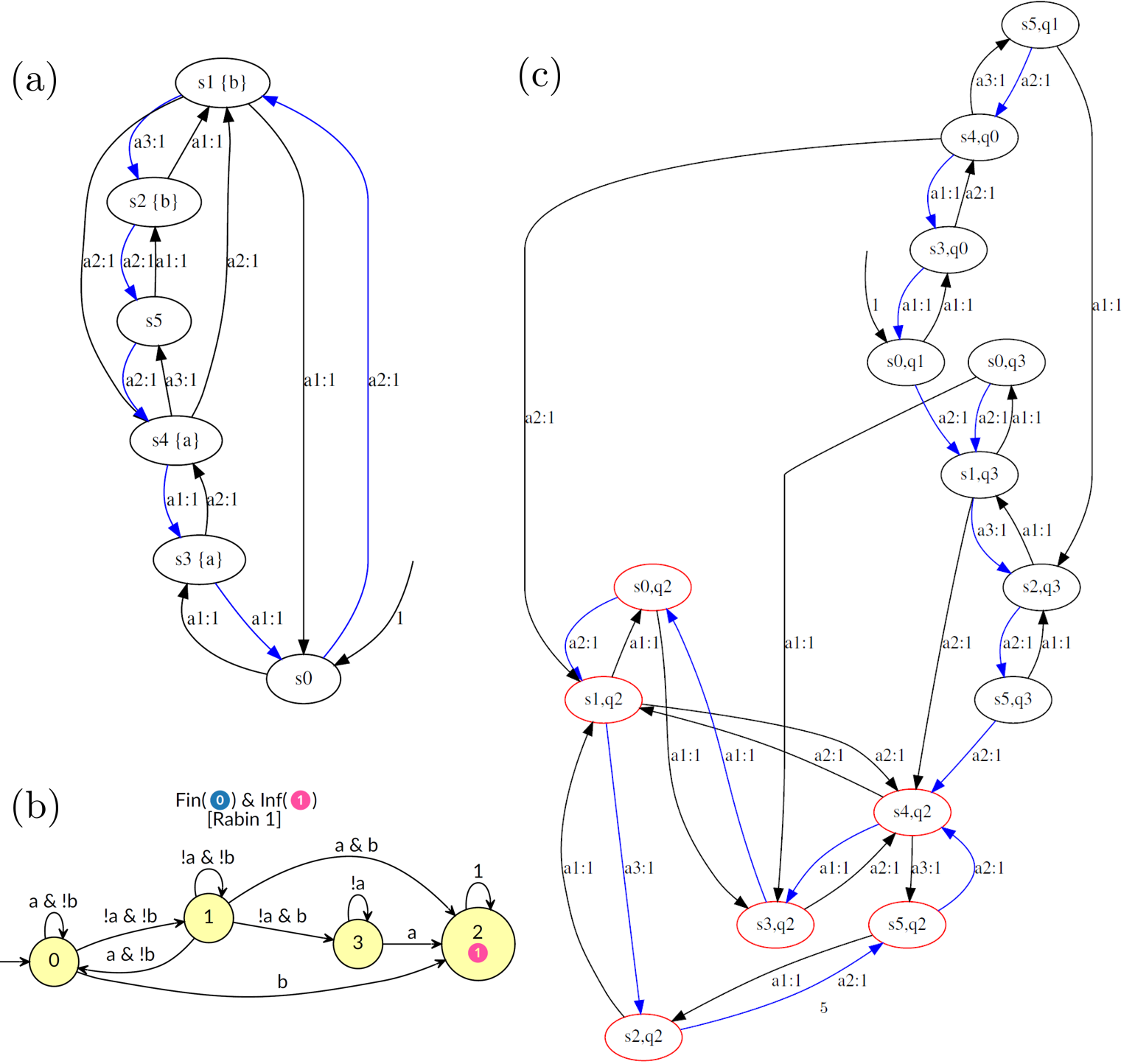
Figure 1: (a) LMDP $\mathcal{M}=(S,\beta,A,T,R=\emptyset,AP,L)$, where $S=\{s_{0},\dots,s_{5}\}$, $\beta(s_{0})=1$, $A=\{a_{1},a_{2},a_{3}\}$, $AP=\{a,b\}$, and $L(s_{1})=L(s_{2})=\{b\},L(s_{3})=L(s_{4})=\{a\}$. The transition function is deterministic (i.e. $T:S\times A\times S\mapsto\{0,1\}$) and shown in the figure by the transitions $a_{i}:1$ between states $s,s^{\prime}$ denoting that $T(s^{\prime}|s,a_{i})=1$. The blue transitions define a policy $\pi:S\times A\mapsto\{0,1\}$ which induces an LMC $\mathcal{M}_{\pi}$. (b) Given the LTL specification $(\textbf{F }a)\textbf{ U }b$, the LTL DRA $\mathcal{A}=(Q,q_{0},\Sigma,\delta,F=\{(J_{i},K_{i})\}_{i})$ is defined, where $Q=\{q_{0},q_{1},q_{2},q_{3}\}$, $\Sigma=2^{AP}$, $F=\{(\emptyset,\{q_{2}\})\}$, and the transition function is given by $\delta(q_{0},\{a\})=q_{0},\delta(q_{0},\emptyset)=q_{1},\delta(q_{0},\{b\})=q_{2},\delta(q_{1},\{a\})=q_{0},\delta(q_{1},\emptyset)=q_{1},\delta(q_{1},\{b\})=q_{3},\delta(q_{3},\{a\})=q_{2},\delta(q_{3},\{b\}),\delta(q_{3},\{a\})=q_{2},\delta(q_{2},\cdot)=q_{2}$. (c) Product LMDP $\mathcal{M}\times\mathcal{A}$, where red nodes represent states in the accepting MEC of $\mathcal{M}\times\mathcal{A}$. The blue transitions define the LMC $(\mathcal{M}\times\mathcal{A})_{\pi}$ induced by the policy $\pi$ given by the blue transitions in (a) for the LMDP $\mathcal{M}$. Note that this policy induces an LMC that has probability 1 of being trapped in the accepting MEC. Therefore, the probability of satisfying $(\textbf{F }a)\textbf{ U }b$ given that we start in state $s_{0}$ is 1.

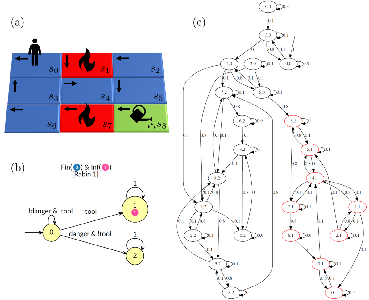
Figure 2: (a) LMDP $\mathcal{M}=(S,\beta,A,T,R=\emptyset,AP,L)$, where $S=\{s_{0},\dots,s_{8}\}$, $\beta(s_{0})=1$, $A=\{\leftarrow,\downarrow,\rightarrow,\uparrow\}$, $AP=\{home,danger,tool\}$, and $L(s_{0})=\{home\},L(s_{1})=L(s_{7})=\{danger\},L(s_{8})=\{tool\}$. the agent has a chance of slipping whenever it moves, causing a transition into one of three possible states. If the agent chooses to go right (left), there is an 80$\%$ chance that it will transition to the right (left), and the chance of transitioning to either of the states above or below it is 10$\%$. Similarly, if the agent chooses to up (down), it will end up in the states above (below) it with 80$\%$ chance, and in the states to the right and left of it with chance 10$\%$ each. In the corners of the map, the agent may stay in place with 90$\%$ probability by choosing to move against the boundary of the map (e.g. $T(s_{0}|s_{0},\leftarrow)=0.9$). (b) Given the SSTL specification $(!danger\textbf{U}tool)\wedge\textbf{SS}_{[0.75,1]}home$, the LTL DRA $\mathcal{A}=(Q,q_{0},\Sigma,\delta,F=\{(J_{i},K_{i})\}_{i})$ is defined, where $Q=\{q_{0},q_{1},q_{2}\}$, $\Sigma=2^{AP}$, $F=\{(\emptyset,\{q_{1}\})\}$, and the transition function is given by $\delta(q_{0},\{home\})=q_{0},\delta(q_{0},\{tool\})=q_{1},\delta(q_{0},\{danger\})=q_{2},\delta(q_{1},\cdot)=q_{1},\delta(q_{2},\cdot)=q_{2}$. The steady-state operator is not used in defining $\mathcal{A}$. (c) Product LMC $(\mathcal{M}\times\mathcal{A})_{\pi}$ induced by the policy $\pi$ given by the black arrows in (a) for the product LMDP $\mathcal{M}\times\mathcal{A}$, where red nodes represent states in the accepting BSCC of $(\mathcal{M}\times\mathcal{A})_{\pi}$. Note that this policy has non-zero probability of being trapped in the accepting BSCC. Furthermore, note that $\sum_{s\in\mathcal{L}_{home}}\text{Pr}^{\infty}_{\pi}(s)=\text{Pr}^{\infty}_{\pi}(s_{0})=0.76$, thereby satisfying the steady-state specification $\textbf{SS}_{[0.75,1]}home$.

Definition 11 (Maximal End Component).

Given the product LMDP $\mathcal{M}^{\times}=(S^{\times},\beta^{\times},A^{\times},$ $T^{\times},Q,L^{\times})$ of an LMDP $\mathcal{M}=(S,\beta,A,T,AP,L)$ and a DRA $\mathcal{A}=\left(Q,q_{0},\Sigma=2^{AP},\delta,\right.$ $\left.\{(J_{i},K_{i})\}_{i\in[m]}\right)$, an end component $E=(S^{E},A^{E}),S^{E}\subseteq S^{\times},A^{E}(s)\subseteq A^{\times}(s)$ is a sub-MDP of $\mathcal{M}$ such that the digraph formed by $E$ is strongly connected. An end component is said to be maximal if it is not contained in any other end component.

Definition 12 (Accepting Maximal End Component (principlesOfModelChecking)).

An accepting maximal end component $E=(S^{E},A^{E})$ is a maximal end component of $\mathcal{M}^{\times}$ such that $S^{E}\cap(S\times J_{i})=\emptyset$ and $S^{E}\cap(S\times K_{i})\neq\emptyset$ for some $i\in[m]$.

As with LMDPs and LMCs, any solution policy $\pi$ induces a product LMC in the underlying product LMDP. These LMCs have analogues to the maximal end components of LMDPs, known in this case as accepting bottom strongly connected components. See Figure 2 for an example.

Definition 13 (Product LMC).

Given an LMC $\mathcal{M}=(S,\beta,T,AP,L)$ and a DRA $\mathcal{A}=(Q,q_{0},\Sigma=2^{AP},\delta,{(J_{i},K_{i})}_{i\in[m]})$, the product Markov chain is given by $\mathcal{M}\times\mathcal{A}=(S^{\times},\beta^{\times},T^{\times},$ $Q,L^{\times})$, where $L^{\times}((s,q))=\{q\}$ and $\beta^{\times},T^{\times}$ are given by:

$$\begin{aligned} \beta^{\times}((s,q))=\begin{cases}\beta(s)&q=\delta(q_{0},L(s))\\ 0&\text{otherwise}\end{cases}\\ T^{\times}((s^{\prime},q^{\prime})|(s,q))=\begin{cases}T(s^{\prime}|s)&q^{\prime}=\delta(q,L(s^{\prime}))\\ 0&\text{otherwise}\end{cases}\\ \end{aligned}$$

Definition 14 (Bottom Strongly Connected Component).

Given an LMC $\mathcal{M}=(S,\beta,T,AP,$ $L)$, a Bottom Strongly Connected Component (BSCC) is a closed strongly connected component $S^{B}\subseteq S$. That is, one which, when entered, is never left.

Definition 15 (Accepting BSCC).

Given a product LMC $\mathcal{M}\times\mathcal{A}=(S^{\times},\beta^{\times},T^{\times},Q,L^{\times})$ of LMC $\mathcal{M}=(S,\beta,T,AP,L)$ and DRA $\mathcal{A}=(Q,q_{0},\Sigma=2^{AP},\delta,\{J_{i},K_{i}\}_{i\in[m]})$, an accepting BSCC $S^{B}\subseteq S^{\times}$ of $\mathcal{M}\times\mathcal{A}$ is a BSCC such that, for some $i\in[m]$, we have $S^{B}\cap(S\times J_{i})=\emptyset$ and $S^{B}\cap(S\times K_{i})\neq\emptyset$.

There is a one-to-one correspondence between the probability of an LMC $\mathcal{M}$ satisfying a given LTL specification $\phi$ and the probability of reaching some accepting BSCC in the product LMC $\mathcal{M}\times\mathcal{A}$, where $\mathcal{A}$ is the DRA corresponding to $\phi$.

Given an LMDP $\mathcal{M}=(S,\beta,A,T,R,\Sigma,L)$, the maximum probability of a state $s$ satisfying a given linear-time property $\phi$ can be reduced to the problem of determining the maximum probability of reaching an accepting MEC in the product MDP $\mathcal{M}^{\times}$ of $\mathcal{M}$ and the DRA corresponding to $\phi$. Indeed, it has been shown that, given an arbitrary LTL formula $\phi$ and LMDP $\mathcal{M}$, the policy which maximizes the probability of reaching an accepting MEC in $\mathcal{M}^{\times}$ also yields a policy which maximizes the probability of satisfying $\phi$ in $\mathcal{M}$ (maxProbs). Once an accepting MEC is reached, one must simply choose actions in the MEC infinitely often in order to ensure that all states within it are visited infinitely often. It is worth noting that the policy $\pi:S\times A\rightarrow\{0,1\}$ which maximizes the probability of satisfying $\phi$ for the original LMDP $\mathcal{M}$ can be trivially determined from $\pi^{\times}$ as it has been shown that $\pi(a|s)=\pi^{\times}(a|(s,q)),s\in S,q\in Q$  (CITE).

There is a crucial distinction to be made at this point. Whereas traditional LTL controller synthesis is agnostic to the actions taken when the agent reaches an AMEC, the addition of steady-state specifications makes such choice of actions critical as these can clearly affect the resulting steady-state probabilities of the Markov chain induced by the solution policy. For the remainder of this paper, we focus on the derivation of optimal policies which satisfy a logic fragment of SSTL, which we call SSTL_⟂, wherein the steady-state operator SS cannot be nested within path operators. That is, an SSTL_⟂ formula takes the form of $\theta=\phi_{\text{LTL}}\wedge\bigwedge_{i}\textbf{SS}_{l_{i},u_{i}}p_{i}$.

SSTL_⟂ Controller Synthesis

To preface the process of deriving policies which satisfy steady-state specifications, let us first consider an agent whose goal it is to maximize the expected reward in a product MDP. In the case of unichain MDPs, the program below suffices to compute the optimal policy such that the solution this program yields the identity $x_{sqa}=\pi(a|s)\text{Pr}^{\infty}(s,q)=\pi(a|s)\sum_{a}x_{sqa}$ and the stochastic policy can then be derived from this equation. Such approaches have been proposed for standard unichain MDPs CITE.

$$\begin{aligned} \max&\sum_{(s,q)\in S^{\times}}\sum_{a\in A(s)}x_{sqa}\sum_{s^{\prime}\in S}T(s^{\prime}|s,a)R(s,a,s^{\prime})\hskip 12.0pt\text{subject to}\\ (i)\text{ }&\sum_{(s,q)\in S^{\times}}\sum_{a\in A(s)}x_{sqa}T^{\times}((s^{\prime},q^{\prime})|(s,q),a)=\sum_{a\in A(s^{\prime})}x_{s^{\prime}q^{\prime}a}\\ &\hskip 168.0pt\forall(s^{\prime},q^{\prime})\in S^{\times}\\ (ii)\text{ }&\sum_{(s,q)\in S^{\times}}\sum_{a\in A(s)}x_{sqa}=1\\ \end{aligned}$$

However, consider the more general case where the given MDP may be multichain and we wish to derive an optimal deterministic policy. Two key problems arise. First, there is no assumption that every policy will yield a Markov chain with a single BSCC as per the unichain condition. As such, we must search for such a policy, if one exists, by enforcing the existence of such a BSCC through additional constraints. Second, we note the challenges of deriving the correct steady-state distributions for an agent using linear programming in the multichain setting. In particular, the seminal work of Kallenberg CITE demonstrated that there is not a one-to-one correspondence between the steady-state distribution derived from linear programming solutions to expected-reward MDPs and the true steady-state distribution of the agent enacting the resulting policy when the Markov chain is multichain (i.e. contains multiple BSCCs, and possibly some transient states). Though there has been recent progress on this front by focusing on restricted classes of policies CITE-IJCAI2020, this problem persists for general policies. On the other hand, unichains yield a one-to-one correspondence between the solution of the steady-state equations and the true steady-state behavior of the agent. Furthermore, the solution to these equations is unique in said setting. We thus focus on deriving an optimal solution policy which satisfies a given SSTL_⟂ in a (potentially) multichain LMDP such that the induced Markov chain is unichain. The interplay with a product LMDP and product Markov chain introduces some challenges in deriving such a policy. In particular, it may be the case that the product Markov chain induced by the solution policy is multichain and its corresponding original Markov chain is unichain. We present a novel solution which accounts for such settings by forcing all BSCCs in the product multichain to be isomorphic. This then establishes that the original Markov chain is a unichain. We further prove that the steady-state probabilities derived over the former yield a one-to-one correspondence with the true steady-state behavior of the agent in the latter.

First, let us consider the simpler case where the product LMC is a unichain. Note that the single BSCC may contain the same state $s\in S$ multiple times as $(s,q),(s,q^{\prime}),\dots$ We will show that the partition $[s]=\{(s,q)\}_{q}$ naturally defined over the product LMC to yield the original Markov chain is such that $\text{Pr}^{\infty}(s)=\sum_{(s,q)\in[s]}\text{Pr}^{\infty}(s,q)$. That is, we can compute the steady-state probabilities over the product LMC and use these to derive those in the original Markov chain over which the SSTL_⟂ specification is defined. This is enabled by the lumpability of the product Markov chain. Some definitions are in order.

Definition 16 (Lumpability).

((lumpability), Definition 1) Given an irreducible Markov chain $M=(S,T)$ and a partition $\bigcup_{s\in S}[s]$ of $S$, then $\bigcup_{s\in S}[s]$ is called ordinarily lumpable if and only if $(\mathbf{e}_{\alpha}-\mathbf{e}_{\beta})TV=\mathbf{0}$ for all $s_{\alpha},s_{\beta}\in[s],s\in S$, where $\mathbf{e}$ is the standard basis vector and $V$ is defined so that $v_{ik}=1$ if $s_{i}\in[s_{k}]$ and $v_{ik}=0$ otherwise.

Lemma 1.

Given an arbitrary BSCC $(\hat{S},\hat{T})$ of a product LMC $M^{\times}=(S^{\times},T^{\times}_{\pi})$, the partition $\bigcup_{s\in S}[s]$ given by $[s]=\{(s,q)|(s,q)\in\hat{S}\}$ is ordinarily lumpable.

Proof.

(Sketch) We must show that, for all $s\in\hat{S}$ and all $(s,q_{\alpha}),(s,q_{\beta})\in[s]$, we have $(e_{\alpha}-e_{\beta})\hat{T}V=0$. Let $V\in\{0,1\}^{|S|\times|Q|\times|S|}$ such that $v_{ijk}=1$ if $(s_{i},q_{j})\in[s_{k}]$ and $v_{ijk}=0$ otherwise.

$$(e_{\alpha}-e_{\beta})\hat{T}V=\left(\hat{T}((s,q_{k})|(s,q_{\alpha}))-\hat{T}((s,q_{k})|(s,q_{\beta}))\right)_{k}V$$ (5)

$$=\left(\sum_{ij}v_{ijk}[\hat{T}((s_{i},q_{j})|(s,q_{\alpha}))-\hat{T}((s_{i},q_{j})|(s,q_{\beta}))]\right)_{k}$$

Looking at the $k^{\text{th}}$ entry, we have:

$$\sum_{(s_{i},q_{j})\in[s_{k}]}\hat{T}((s_{i},q_{j})|(s,q_{\alpha}))-\hat{T}((s_{i},q_{j})|(s,q_{\beta}))$$ (6)

Two cases arise. First, let us consider the case where $s\neq s_{k}$. By definition of the quotient LMC, it follows that, for every transition $[s]\rightarrow[s_{k}]$, there are corresponding transitions $(s,q_{\alpha})\rightarrow(s_{k},q_{\alpha^{\prime}})$ and $(s,q_{\beta})\rightarrow(s_{k},q_{\beta^{\prime}})$ such that $\hat{T}((s_{k},q_{\alpha^{\prime}})|(s,q_{\alpha}))=\hat{T}((s_{k},q_{\beta^{\prime}})|(s,q_{\beta}))=T(s_{k}|s)$. Thus, the sum equates to 0 in this case.

Now, assume $s=s_{k}$. Two cases arise. First, let us consider the case where $[s]$ does not contain a self loop in the quotient LMC. Then all terms in the preceding sum (6) are $T(s|s)=0$. Now, let us consider the case where there is a self loop so that $T(s|s)>0$. Then, since the DRA is deterministic, there is exactly one successor $(s,q^{\prime})\in[s]$ for any given $(s,q)\in[s]$. Any trajectory of such product states resulting from the self loop must inevitably revisit some state (mention that this follows from the pumping lemma?), yielding a lollipop walk. For any two states, say $(s,q_{i})$ and $(s,q_{j})$, in this walk, there is exactly one successor yielding the term $T(s|s)$ for each of the two states. Thus, the sum in (6) equates to 0.

Since $s,\alpha,\beta$ were chosen arbitrarily, we have shown that $(e_{\alpha}-e_{\beta})\hat{T}V=0$. ∎

Theorem 1.

((lumpabilityOriginal), (lumpability), Theorem 4) Given a Markov chain $M^{\prime}=(S^{\prime},T^{\prime})$ and an ordinarily lumpable partition $\bigcup_{s^{\prime}\in S^{\prime}}[s^{\prime}]$ of $S^{\prime}$, the steady-state distribution of the aggregated Markov chain $M=(S,T)$ satisfies $\text{Pr}^{\infty}(s)=\sum_{s^{\prime}\in[s]}\text{Pr}^{\infty}(s^{\prime})$ for every $s\in S$. Furthermore, the transition function of the aggregated MC is given by $T(s^{\prime}|s)=\mathbf{e}_{i}T([s^{\prime}]|[s])\mathbf{e}^{T}$, where $i$ can be the index of any $(s,\cdot)\in S^{\times}$.

Corollary 1.

Given an irreducible product LMC, the original LMC is the aggregated MC resulting from the ordinarily lumpable partition.

Proof.

(Sketch) Easy to show that $T(s^{\prime}|s)=\mathbf{e}_{i}T([s^{\prime}]|[s])\mathbf{e}^{T}$.

$$T([s^{\prime}]|[s])=\left(\begin{smallmatrix}T^{\times}((s^{\prime},q_{1})|(s,q_{1}))&T^{\times}((s^{\prime},q_{2})|(s,q_{1}))&\cdots\\ T^{\times}((s^{\prime},q_{1})|(s,q_{2}))&T^{\times}((s^{\prime},q_{2})|(s,q_{2}))&\cdots\\ \vdots&\vdots&\ddots\end{smallmatrix}\right)$$ (7)

∎

The previous theorem and corollary establish the one-to-one correspondence between the steady-state probabilities derived for a unichain LMC and the steady-state distribution for the original LMC. Now, let us consider the case where the product LMC is a multichain. We establish sufficient conditions for establishing the same one-to-one correspondence of steady-state distributions.

Lemma 2.

Let $\pi$ denote a policy and $M_{\pi}=(S,T_{\pi})$ denote the Markov chain induced by this policy such that $M_{\pi}$ satisfies $\phi_{\text{LTL}}$. Let $(S^{k})_{k}$ denote the BSCCs in the product MC induced by $\pi$. Then $M_{\pi}$ is a unichain if and only if some state $(s,\cdot)\in S^{\times}$ shows up in every BSCC $S^{k}$ of the product LMC.

Proof.

(Sketch) ($\implies$) Assume $M_{\pi}$ is a unichain. From the one-to-one correspondence of paths between the LMC and product LMC, it follows that all BSCCs in the product LMC must be the same. ($\impliedby$) If some state is shared across all BSCCs in the product LMC, then, by the one-to-one correspondence between path in $M_{\pi}$ and paths in $M^{\times}_{\pi}$, it follows that $M_{\pi}$ is irreducible. Furthermore, its single BSCC $S^{\prime}$ is such that $S^{\prime}=S^{k}$ for all $k$. ∎

Lemma 3.

Given a multichain $M=(S,T)$ with $m$ identical BSCCs given by transition probability matrices $T_{1},\dots,T_{m}$ (That is, the graph structures of these components are all isomorphic) and an irreducible Markov chain $M^{*}=(S^{*},T^{*})$, where $S^{*}$ contains exactly the states in the first BSCC and $T^{*}=T_{1}$ (without loss of generality), the steady-state probability of an arbitrary state $(s,q)\in S^{*}$ is equivalent to the sum of steady-state probabilities of all states isomorphic to it in $S$.

Proof.

The transition probability matrix $T$ is given by the canonical form in equation (8) (puterman1994markov), where $W_{k}$ denotes transitions from transient states to the $k^{\text{th}}$ BSCC and $Z$ denotes transitions between transient states.

$$T=\begin{bmatrix}T_{1}&0&\ldots&0&0\\ 0&T_{2}&\dots&0&0\\ \vdots&\vdots&\ddots&\vdots&\vdots\\ 0&0&\ldots&T_{m}&0\\ W_{1}&W_{2}&\ldots&W_{m}&Z\end{bmatrix}$$ (8)

Recall the steady-state equations given below for the product LMC $M$.

$$(\text{Pr}^{\infty}(s_{0},q_{0}),\dots)T =(\text{Pr}^{\infty}(s_{0},q_{0}),\dots)$$

$$\sum_{(s,q)\in S^{\times}}\text{Pr}^{\infty}(s,q) =1$$

This yields the following system of linear equations for $M$:

$$\text{Pr}^{\infty}(s,q)=\sum_{(s^{\prime},q^{\prime})\in S^{*}}\text{Pr}^{\infty}(s^{\prime},q^{\prime})T(s,q|s^{\prime},q^{\prime})\hskip 12.0pt\forall(s,q)\in S^{*}$$

$$\sum_{(s,q)\in S^{*}}\!\!\!\!\text{Pr}^{\infty}(s,q)=1$$

Similarly, we have the following equations for $M^{*}$:

$$\text{Pr}^{\infty}(s,q)=\!\!\!\!\sum_{(s^{\prime},q^{\prime})\in S^{k}}\!\!\!\!\text{Pr}^{\infty}(s^{\prime},q^{\prime})T(s,q|s^{\prime},q^{\prime})\hskip 12.0pt\forall(s,q)\in S^{k},k$$

$$\sum_{k\in[m]}\sum_{(s,q)\in S^{k}}\!\!\!\!\text{Pr}^{\infty}(s,q)=1$$

Let $\langle s\rangle=\{(s,q)|(s,q)\text{ isomorphic in }T^{G}_{1},\dots,T^{G}_{m}\}$, where $T^{G}_{k}$ denotes the graph structure of $T_{k}$. It follows that

$$\sum_{(s,q)\in S^{*}}\!\!\!\!\text{Pr}^{\infty}(s,q)=$$

$$\sum_{(s,q)\in S^{*}}\sum_{(s^{\prime},q^{\prime})\in S^{*}}\text{Pr}^{\infty}(s^{\prime},q^{\prime})T(s,q|s^{\prime},q^{\prime})=1=$$

$$\sum_{k\in[m]}\sum_{(s,q)\in S^{k}}\!\!\!\!\text{Pr}^{\infty}(s,q)=$$

$$\sum_{k\in[m]}\sum_{(s,q)\in S^{k}}\sum_{(s^{\prime},q^{\prime})\in S^{k}}\!\!\!\!\text{Pr}^{\infty}(s^{\prime},q^{\prime})T(s,q|s^{\prime},q^{\prime})=$$

$$\sum_{(s,q)\in S^{1}}\sum_{(s^{\prime},q^{\prime})\in S^{1}}T(s,q|s^{\prime},q^{\prime})\sum_{(s^{\prime\prime},q^{\prime\prime})\in\langle s^{\prime}\rangle}\!\!\!\!\text{Pr}^{\infty}(s^{\prime\prime},q^{\prime\prime})$$

Note that the choice of $S^{1}$ in the last equation is arbitrary. Therefore, $\text{Pr}^{\infty}(s,q)=\sum_{(s^{\prime},q^{\prime})\in\langle s\rangle}\text{Pr}^{\infty}(s^{\prime},q^{\prime})$ for all $(s,q)\in S^{*}$. ∎

The preceding lemma and Theorems 1 and 2 establish necessary and sufficient conditions for a multichain product LMC to yield a unichain in the original LMDP such that there is a one-to-one correspondence between the sum of steady-state probabilities $\sum_{q}\text{Pr}^{\infty}(s,q)$ in the former and the steady-state distribution $\text{Pr}^{\infty}(s)$ in the latter.

We can now add constraints to ensure that the solution policy is deterministic and yields a unichain in the original LMDP even though the product LMC induced in the product LMDP may be multichain. Constraint (iii) ensures that a positive occupation measure implies that the action corresponding to it is selected as part of the solution policy.

$$\begin{aligned} (iii)\text{ }&x_{sqa}\leq\pi(a|s)&\forall(s,q)\in S^{\times},a\in A\\ (iv)\text{ }&\sum_{a\in A(s)}\pi\left(a|s\right)=1&\forall s\in S\\ \end{aligned}$$

Lemma 4.

Let $(x,\pi)$ denote a feasible solution to constraints $(i)$ through $(iv)$ and assume that the Markov chain $M_{\pi}$ induced by $\pi$ is unichain. Then $x_{sqa}=\pi(a|s)\text{Pr}^{\infty}_{\pi}(s,q)=\pi(a|s)\sum_{a}x_{sqa}$ for all recurrent states $(s,q)\in S^{\times}$.

Proof.

Since $\pi(a|s)\in\{0,1\}$ and $x_{sqa}$ must equal $\pi(a|s)\sum_{a}x_{sqa}$, we must show that $x_{sqa}\in\{0,\sum_{a}x_{sqa}\}$ such that $x_{sqa}=\sum_{a}x_{sqa}$ if and only if $\pi(a|s)=1$. By contrapositive, this also establishes that $x_{sa}=0$ if and only if $\pi(a|s)=0$. Note that $\sum_{a}x_{sqa}>0$ because $(s,q)$ is recurrent.

($\implies$) The contrapositive statement $\pi(a|s)=0$ implies $x_{sqa}=0$ follows directly from constraint $(iii)$.

($\impliedby$) Since $\pi(a|s)=1$, it follows from constraint $(iv)$ that $\sum_{a^{\prime}\in A\setminus\{a\}}\pi(a^{\prime}|s)=0$. From constraint $(iii)$, we then have $\sum_{a^{\prime}\in A\setminus\{a\}}x_{sqa^{\prime}}=0$. It follows that $x_{sqa}=\sum_{a}x_{sqa}$.

From the preceding arguments, we have $x_{sqa}=\pi(a|s)\text{Pr}^{\infty}_{\pi}(s,q)$. From the unichain condition, we further have that there is a unique solution to constraints $(i)$ and $(ii)$. Thus, $\pi$ is the policy which yields the steady-state distribution given by the solution to constraints $(i)$ through $(iv)$. ∎

We can now add additional constraints which utilize the policy $\pi$ in constraints $(iii)$ and $(iv)$ in order to establish that some accepting state within an accepting MEC is reached by this policy and visited infinitely often. This would, in turn, satisfy the path operators of the given SSTL_⟂ formula. In order to ensure that there is a path from the initial state $(s_{0},\delta(q_{0},L(s_{0})))\in S^{\times}$ to a recurrent component in $B^{\times}$ which contains nodes in $\bigcup_{i}K_{i}$ (i.e. nodes that are part of the deterministic Rabin automaton acceptance pairs), we will use flow transfer constraints. This notion of flow reflects the probability of transitioning between states given a policy. Constraint $(v)$ sets the flow capacities. Constraint $(vi)$ ensures that, for every state (except the starting state), if there is incoming flow, then it is strictly greater than the outgoing flow. Put differently, there cannot be outgoing flow unless there is incoming flow. If there is no incoming flow, then there is no outgoing flow and $\mathcal{I}_{sq}$ must necessarily be zero per constraint $(vi)$. Constraint $(vii)$ ensures that, if there is incoming flow into a state $(s,q)\in S^{\times}$, then $\mathcal{I}_{sq}=1$. Constraint $(viii)$ ensures that, whenever there is incoming flow, there must also be some arbitrary amount of outgoing flow. The choice of denominator 2 here is arbitrary.

$$\begin{aligned} (v)\text{ }&f_{sqs^{\prime}q^{\prime}}\leq\sum_{a\in A(s)}T((s^{\prime},q^{\prime})|(s,q),a)\pi(a|s)\\ &\hskip 128.0pt\forall((s,q),(s^{\prime},q^{\prime}))\in T^{G}\\ (vi)\text{ }&\sum_{((s^{\prime},q^{\prime}),(s,q))\in T^{G}}f_{s^{\prime}q^{\prime}sq}\geq\sum_{((s,q),(s^{\prime},q^{\prime}))\in T^{G}}f_{sqs^{\prime}q^{\prime}}+\epsilon\mathcal{I}_{sq}\\ &\hskip 88.0pt\forall(s,q)\in S^{\times}\setminus\{(s_{0},\delta(q_{0},L(s_{0})))\}\\ (vii)\text{ }&\sum_{((s^{\prime},q^{\prime}),(s,q))\in T^{G}}f_{s^{\prime}q^{\prime}sq}\leq\mathcal{I}_{sq}\hskip 48.0pt\forall(s,q)\in S^{\times}\\ (viii)\text{ }&\sum_{((s,q),(s^{\prime},q^{\prime}))\in T^{G}}f_{sqs^{\prime}q^{\prime}}\geq\sum_{((s^{\prime},q^{\prime}),(s,q))\in T^{G}}f_{s^{\prime}q^{\prime}sq}/2\\ &\hskip 168.0pt\forall(s,q)\in S^{\times}\\ \end{aligned}$$ (9)

Constraint $(ix)$ ensures that steady-state probabilities for states with no incoming flow (as determined by $\mathcal{I}_{sq}$ in constraint $(vi)$) is 0. This makes it so that isolated BSCCs do not contribute to the steady-state distribution. Constraint $(x)$ encodes the steady-state specifications given by operators SS and constraint and constraint $(xi)$ ensures that we visit some state in the acceptance pairs $\bigcup_{i}K_{i}$ infinitely often in order to satisfy the given LTL specification. We include constraint $(xi)$ for completeness, but note that $(xi)$ is itself a steady-state specification of the form $\mathbf{SS}_{(0,1]}\bigcup_{i}K_{i}$ (Not exactly true… need to change this) which could be subsumed by $(x)$.

$$\begin{aligned} (ix)\text{ }&\sum_{a\in A(s)}x_{sqa}\leq\mathcal{I}_{sq}&\forall(s,q)\in S^{\times}\\ (x)\text{ }&l\leq\sum_{s\in L^{-1}(\psi)}\sum_{q\in Q}\sum_{a\in A(s)}x_{sqa}\leq u&\forall\textbf{SS}_{[l,u]}\psi\in\theta\\ (xi)\text{ }&\sum_{s\in S}\sum_{q\in\bigcup_{i}K_{i}}\sum_{a\in A(s,q)}x_{sqa}>0\\ \end{aligned}$$ (10)

Recall that the steady-state equations in contraints $(i)$ and $(ii)$ yield the correct steady-state distribution only if there is a single BSCC or if all BSCCs are isomorphic. We must therefore ensure that, in the product LMC, all BSCCs are isomorphic. The one-to-one correspondence of paths between the LMC and the product LMC will then guarantee that the former is unichain even if the latter is not. To accomplish this, we define three indicator variables $\mathcal{I}_{s},\mathcal{I}^{k},\mathcal{I}^{k}_{s}\in\{0,1\}$ which are 1 iff $(s,\cdot)$ shows up in some BSCC of the product LMC, AMEC_k has some state with positive steady-state probability (meaning that it, or a subset of it, will show up as a BSCC in the product LMC), and $(s,\cdot)$ has positive steady-state probability in AMEC_k, respectively. Constraint $(xii)$ ensures that $\mathcal{I}^{k}$ is 1 if some state in AMEC_k has positive steady-state probability.

Constraint $(xiv)$ ensures that, for a given state $s\in S$ and AMEC $k$, if some indicator variable $\mathcal{I}_{sq}$ is 1, then $\mathcal{I}^{k}_{s}$ must be 1. Constraint $(xv)$ ensures that, if $\mathcal{I}_{s}$ is 1, then $(s,\cdot)$ shows up in every BSCC in the product LMC, thereby enforcing that all BSCCs in the solution LMC are isomorphic. Note that the sum $\sum_{k}(\mathcal{I}^{k}_{s}-\mathcal{I}^{k})$ is always non-positive and dividing by the number of AMECs bounds this result to be within $[-1,0]$. Finally, constraint $(xvi)$ ensures that some such state exists.

$$\begin{aligned} (xii)\text{ }&\sum_{(s,q)\in AMEC_{k}}\sum_{a}x_{sqa}\leq\mathcal{I}^{k}&\forall k\\ (xiii)\text{ }&\mathcal{I}^{k}_{s}\leq\sum_{(s,q)\in AMEC_{k}}\mathcal{I}_{sq}&\forall s\in S,k\\ (xiv)\text{ }&\sum_{(s,q)\in AMEC_{k}}\frac{\mathcal{I}_{sq}}{|Q|}\leq\mathcal{I}^{k}_{s}&\forall s\in S,k\\ (xv)\text{ }&\mathcal{I}_{s}-1\leq\frac{\sum_{k}\left(\mathcal{I}^{k}_{s}-\mathcal{I}^{k}\right)}{\#ofAMECs}&\forall s\in S\\ (xvi)\text{ }&\sum_{s}\mathcal{I}_{s}\geq 1\\ \end{aligned}$$ (11)

The program is summarized below and its full definition can be found in the Appendix.

$$\max\sum_{(s,q)\in S^{\times}}\sum_{a\in A(s)}x_{sqa}\sum_{s^{\prime}\in S} T(s^{\prime}|s,a)R(s,a,s^{\prime})$$ (12)

$$\text{subject to }(i)-(xvi)$$

$$x_{sqa},f_{sqs^{\prime}q^{\prime}}\in[0,1] \forall((s,q),a,(s^{\prime},q^{\prime}))\in S^{\times}\times A\times S^{\times}$$

$$\pi(a|s),\mathcal{I}_{sq},\mathcal{I}_{s},\mathcal{I}^{k},\mathcal{I}^{k}_{s}\in\{0,1\} \forall((s,q),a)\in S^{\times}\times A$$

Theorem 2.

Given an LMDP $\mathcal{M}=(S,\beta,A,T,R,AP,L)$ and an SSTL_⟂ objective $\theta=\phi_{\text{LTL}}\wedge\bigwedge_{i}\textbf{SS}_{[l_{i},u_{i}]}p_{i}$ (i.e. an SSTL specification where the SS cannot be nested within LTL operators), let $(x,f,\pi,\mathcal{I})$ denote an assignment to the variables in program (Experimental Results). Then $(x,f,\pi,\mathcal{I})$ is a feasible solution if and only if $\mathcal{M}_{\pi}=(S_{\pi},\beta,T_{\pi},AP,L)$ satisfies $\theta$ and is a unichain.

Proof.

($\implies$) Since the solution $(x,f,\pi,\mathcal{I})$ is feasible, there must be some $(s,q)\in S\times\bigcup_{i}K_{i}$ such that constraint $(xi)$ is satisfied. From constraint $(ix)$, note that this is only possible if $\mathcal{I}_{sq}=1$, which is only possible if there is incoming flow into $(s,q)$ per the flow variables $f_{s^{\prime}q^{\prime}sq}$ in constraint $(vi)$. This corresponds to the outgoing flow of some neighboring state $(s^{\prime},q^{\prime})$. Again, from constraint $(viii)$, it follows that $(s^{\prime},q^{\prime})$ must also have incoming flow. By induction, we see that this holds for all states leading from the initial state $(s_{0},\delta(q_{0},L(s_{0})))$ to $(s,q)$. Since positive flow is only enabled along edges corresponding to actions chosen by the solution policy $\pi$ (per constraint $(v)$), it follows that there is a path from $(s_{0},\delta(q_{0},L(s_{0})))$ to $(s,q)$ in the product LMC and, due to the one-to-one correspondence between paths in the product LMC the original LMC, there is also a path from $s_{0}$ to $s$ in the latter. Now, consider the policy defined at state $(s,q)$. Since there is incoming flow, it follows from constraint $(viii)$ that there must also be outgoing flow. This flow will continue from state to state until some state is revisited, creating a BSCC. Constraints $(xii)$ through $(xvi)$ ensure that all such BSCCs contain the same states. In particular, note that the satisfaction of constraint $(xi)$ yields $\mathcal{I}^{k}=1$ for the $k^{\text{th}}$ AMEC (without loss of generality) within which state $(s,q)$ resides per constraint $(xii)$. Similarly, since $\mathcal{I}_{sq}=1$, it follows from constraint $(xiv)$ that $\mathcal{I}^{k}_{s}=1$ for that same AMEC. Constraint $(xiii)$ ensures that $\mathcal{I}^{k}_{s}$ cannot be set to $1$ unless there is some $\mathcal{I}_{sq}=1$. Thus, for any state $s\in S$ and $k$, we have $\mathcal{I}^{k}_{s}\leq\mathcal{I}^{k}$ and this is only met with equality if state $s\in S$ shows up in BSCC $k$. It follows that the sum $\sum_{k}(\mathcal{I}^{k}_{s}-\mathcal{I}^{k})$ on the RHS of constraint $(xv)$ achieves its maximum value of $0$ if and only if state $s$ shows up in every BSCC of the product LMC. This must be the case per constraint $(xvi)$, which forces the LHS of constraint $(xv)$ to be $0$ for some state. From Lemma 2, this yields a unichain in the original LMDP. From Theorem 1 and Lemma 3, the satisfaction of constraint $(x)$ yields an LMC which satisfies the steady-state specifications in $\theta$.

($\impliedby$) Assume we have a policy $\pi$ and the unichain induced by $\pi$ is given by $\mathcal{M}_{\pi}=(S,T_{\pi})$ and satisfies the given SSTL_⟂ specification. We derive a feasible solution $(x,f,\pi,\mathcal{I})$ to program (Experimental Results) in the sequel. It follows from Lemma 2 that all BSCCs in $(\mathcal{M}\times A)_{\pi}$ must contain the same states in $S$. That is, $S^{k}=S^{k^{\prime}}$ for all BSCCs in the product LMC. Let $\mathcal{I}_{sq}=\mathcal{I}_{s}=\mathcal{I}^{k}=\mathcal{I}^{k}_{s}=1$ for all states $(s,q)$ in the BSCC corresponding to enabled AMEC $k$ (for all $k$). This satisfies constraints $(xii)$ through $(xvi)$. Note that the steady-state probabilities of such states must be positive and we can assign these values to $\sum_{a}x_{sqa}$ for every $(s,q)$ in the BSCCs. This satisfies $(i),(ii)$, and $(ix)$. Since the SSTL_⟂ specification is satisfied, it must be the case that some state $(s,q)\in S\times\bigcup_{i}K_{i}$ is visited infinitely often, so we can assign the steady-state probability of such states to the sum of variables $\sum_{a}x_{sqa}$, thereby satisfying $(xi)$. Furthermore, since the steady-state operators in the specification are satisfied, it follows from Theorem 1 that constraint $(x)$ is satisfied. Note that constraints $(v)$ through $(viii)$ can be satisfies by setting the flow values to be proportional to the policy values. ∎

Experimental Results

Simulations of program (Experimental Results) were performed using CPLEX version $12.8$ (CPLEX) on a machine with a $3.6$ GHz Intel Core i7-6850K processor and $128$ GB of RAM. There are four actions corresponding to the four cardinal directions and a deterministic transition function $T:S\times A\times S\mapsto\{0,1\}$ defined in the obvious manner. Each state-action pair observes a uniformly distributed random reward in $\{0,1\}$. There are four labels $a,b,c,d$, each allocated to one-fourth of the states chosen at random. See Table 1 for runtime results.

$$\begin{aligned} \theta_{1}&=(\mathbf{G}\neg b)\wedge(\mathbf{G}\mathbf{F}a)\wedge\textbf{SS}_{[0.01,0.5]}d\\ \theta_{2}&=(\mathbf{G}\mathbf{F}a)\vee(\mathbf{F}\mathbf{G}b)\wedge\textbf{SS}_{[0.01,0.5]}d\\ \theta_{3}&=(\mathbf{F}\mathbf{G}a)\mathbf{U}(b\vee\mathbf{X}(b\vee\mathbf{X}(b\vee\mathbf{X}b)))\wedge\textbf{SS}_{[0.01,0.5]}d\\ \theta_{4}&=(\mathbf{F}a)\mathbf{U}b\wedge\textbf{SS}_{[0.01,0.5]}d\\ \theta_{5}&=(\mathbf{F}a)\wedge\mathbf{F}(a\mathbf{U}b)\wedge\textbf{SS}_{[0.01,0.5]}d\\ \theta_{6}&=\mathbf{F}(a\wedge\mathbf{X}(a\wedge\mathbf{X}a))\wedge\textbf{SS}_{[0.01,0.5]}d\\ \theta_{7}&=(\mathbf{F}a\wedge\mathbf{F}b)\wedge((\mathbf{F}a\wedge\mathbf{F}b)\mathbf{U}(c\vee\mathbf{X}a))\wedge\textbf{SS}_{[0.01,0.5]}d\\ \theta_{8}&=\mathbf{F}a\wedge\mathbf{F}b\wedge\mathbf{F}c\wedge\textbf{SS}_{[0.01,0.5]}d\\ \end{aligned}$$

$\theta$	$4\times 4$	$8\times 8$	$16\times 16$
$\theta_{1}$	$0.45(0.42)$	$25.42(117.31)$	$53.36(120.11)$
$\theta_{2}$	$0.51(0.99)$	$0.15(0.06)$	$1.41(0.53)$
$\theta_{3}$	$0.65(1.61)$	$0.69(0.30)$	$48.54(60.20)$
$\theta_{4}$	$1.00(2.95)$	$1.12(0.50)$	$76.90(68.07)$
$\theta_{5}$	$0.50(1.37)$	$1.59(0.73)$	$139.25(96.10)$
$\theta_{6}$	$0.29(0.61)$	$1.04(0.30)$	$152.93(128.66)$
$\theta_{7}$	$0.55(2.00)$	$4.75(3.03)$	$219.39(158.18)$
$\theta_{8}$	$3.05(8.72)$	$11.06(4.96)$	$369.07(184.75)$

Table 1: Average runtimes and standard deviations for 25 random instances of program (Experimental Results) using CPLEX version $12.8$ for SSTL_⟂ formulas $\theta$ previously listed and for grids of sizes $4\times 4$, $8\times 8$, and $16\times 16$.

$$\begin{aligned} \max&\sum_{(s,q)\in S^{\times}}\sum_{a\in A(s)}x_{sqa}\sum_{s^{\prime}\in S}T(s^{\prime}|s,a)R(s,a,s^{\prime})\hskip 12.0pt\text{subject to}\\ (i)\text{ }&\sum_{(s,q)\in S^{\times}}\sum_{a\in A(s)}x_{sqa}T^{\times}((s^{\prime},q^{\prime})|(s,q),a)=\sum_{a\in A(s^{\prime})}x_{s^{\prime}q^{\prime}a}&\hskip 12.0pt\forall(s^{\prime},q^{\prime})\in S^{\times}\\ (ii)\text{ }&\sum_{(s,q)\in S^{\times}}\sum_{a\in A(s)}x_{sqa}=1\\ (iii)\text{ }&x_{sqa}\leq\pi(a|s)&\forall(s,q)\in S^{\times},a\in A\\ (iv)\text{ }&\sum_{a\in A(s)}\pi\left(a|s\right)=1&\forall s\in S\\ (v)\text{ }&f_{sqs^{\prime}q^{\prime}}\leq\sum_{a\in A(s)}T((s^{\prime},q^{\prime})|(s,q),a)\pi(a|s)&\hskip 12.0pt\forall((s,q),(s^{\prime},q^{\prime}))\in T^{G}\\ (vi)\text{ }&\sum_{((s^{\prime},q^{\prime}),(s,q))\in T^{G}}f_{s^{\prime}q^{\prime}sq}\geq\sum_{((s,q),(s^{\prime},q^{\prime}))\in T^{G}}f_{sqs^{\prime}q^{\prime}}+\epsilon\mathcal{I}_{sq}&\hskip 12.0pt\forall(s,q)\in S^{\times}\setminus\{(s_{0},\delta(q_{0},L(s_{0})))\}\\ (vii)\text{ }&\sum_{((s^{\prime},q^{\prime}),(s,q))\in T^{G}}f_{s^{\prime}q^{\prime}sq}\leq\mathcal{I}_{sq}&\hskip 12.0pt\forall(s,q)\in S^{\times}\\ (viii)\text{ }&\sum_{((s,q),(s^{\prime},q^{\prime}))\in T^{G}}f_{sqs^{\prime}q^{\prime}}\geq\sum_{((s^{\prime},q^{\prime}),(s,q))\in T^{G}}f_{s^{\prime}q^{\prime}sq}/2&\hskip 12.0pt\forall(s,q)\in S^{\times}\\ (ix)\text{ }&\sum_{a\in A(s)}x_{sqa}\leq\mathcal{I}_{sq}&\forall(s,q)\in S^{\times}\\ (x)\text{ }&l\leq\sum_{s\in L^{-1}(\psi)}\sum_{q\in Q}\sum_{a\in A(s)}x_{sqa}\leq u&\forall\textbf{SS}_{[l,u]}\psi\in\theta\\ (xi)\text{ }&\sum_{s\in S}\sum_{q\in\bigcup_{i}K_{i}}\sum_{a\in A(s,q)}x_{sqa}>0\\ (xii)\text{ }&\sum_{(s,q)\in AMEC_{k}}\sum_{a}x_{sqa}\leq\mathcal{I}^{k}&\forall k\\ (xiii)\text{ }&\mathcal{I}^{k}_{s}\leq\sum_{(s,q)\in AMEC_{k}}\mathcal{I}_{sq}&\forall s\in S,k\\ (xiv)\text{ }&\sum_{(s,q)\in AMEC_{k}}\frac{\mathcal{I}_{sq}}{|Q|}\leq\mathcal{I}^{k}_{s}&\forall s\in S,k\\ (xv)\text{ }&\mathcal{I}_{s}-1\leq\frac{\sum_{k}\left(\mathcal{I}^{k}_{s}-\mathcal{I}^{k}\right)}{\#ofAMECs}&\forall s\in S\\ (xvi)\text{ }&\sum_{s}\mathcal{I}_{s}\geq 1\\ &x_{sqa},f_{sqs^{\prime}q^{\prime}}\in[0,1]&\forall((s,q),a,(s^{\prime},q^{\prime}))\in S\times A\times S^{\times}\\ &\mathcal{I}_{sq},\mathcal{I}_{s},\mathcal{I}^{k},\mathcal{I}^{k}_{s}\in\{0,1\}&\forall((s,q),a)\in S^{\times}\times A\\ \end{aligned}$$

$$\begin{aligned} \max&\sum_{(s,q)\in S^{\times}}\sum_{a\in A(s)}x_{sqa}\sum_{s^{\prime}\in S}T(s^{\prime}|s,a)R(s,a,s^{\prime})\hskip 12.0pt\text{subject to}\\ (i)\text{ }&z_{s_{0},\delta(q_{0},L(s_{0}))}=1\\ (ii)\text{ }&z_{sq}=\sum_{(s^{\prime},q^{\prime})\in S^{\times}}\sum_{a\in A(s)}T^{\times}((s^{\prime},q^{\prime})|(s,q),a)w_{sas^{\prime}q^{\prime}}&\forall(s,q)\in S^{\times}\setminus(B^{\times}\cup C^{\times})\\ (iii)\text{ }&w_{sas^{\prime}q^{\prime}}\leq\pi(a|s)&\forall(s,a,(s^{\prime},q^{\prime}))\in S\times A\times S^{\times}\\ (iv)\text{ }&w_{sas^{\prime}q^{\prime}}\leq z_{s^{\prime}q^{\prime}}&\forall(s,a,(s^{\prime},q^{\prime}))\in S\times A\times S^{\times}\\ (v)\text{ }&w_{sas^{\prime}q^{\prime}}\geq z_{s^{\prime}q^{\prime}}+\pi(a|s)-1&\forall(s,a,(s^{\prime},q^{\prime}))\in S\times A\times S^{\times}\\ (vi)\text{ }&\sum_{(s,q)\in B^{\times}}z_{sq}=|B^{\times}|\\ (vii)\text{ }&\sum_{(s,q)\in C^{\times}}z_{sq}=0\\ (viii)\text{ }&\sum_{a\in A(s)}\pi\left(a|s\right)=1&\forall s\in S\\ (ix)\text{ }&\sum_{(s,q)\in S^{\times}}\sum_{a\in A(s)}x_{sqa}T^{\times}((s^{\prime},q^{\prime})|(s,q),a)=\sum_{a\in A(s^{\prime})}x_{s^{\prime}q^{\prime}a}&\hskip 12.0pt\forall(s^{\prime},q^{\prime})\in S^{\times}\\ (x)\text{ }&\sum_{(s,q)\in S^{\times}}\sum_{a\in A(s)}x_{sqa}=1\\ (xi)\text{ }&x_{sqa}\leq\pi(a|s)&\forall(s,q)\in S^{\times},a\in A\\ (xii)\text{ }&f_{sqs^{\prime}q^{\prime}}\leq\sum_{a\in A(s)}T((s^{\prime},q^{\prime})|(s,q),a)\pi(a|s)&\hskip 12.0pt\forall((s,q),(s^{\prime},q^{\prime}))\in T^{G}\\ (xiii)\text{ }&\sum_{((s^{\prime},q^{\prime}),(s,q))\in T^{G}}f_{s^{\prime}q^{\prime}sq}\geq\sum_{((s,q),(s^{\prime},q^{\prime}))\in T^{G}}f_{sqs^{\prime}q^{\prime}}+\epsilon\mathcal{I}_{sq}&\hskip 12.0pt\forall(s,q)\in S^{\times}\setminus\{(s_{0},\delta(q_{0},L(s_{0})))\}\\ (xiv)\text{ }&\sum_{((s^{\prime},q^{\prime}),(s,q))\in T^{G}}f_{s^{\prime}q^{\prime}sq}\leq\mathcal{I}_{sq}&\hskip 12.0pt\forall(s,q)\in S^{\times}\\ (xv)\text{ }&\sum_{((s,q),(s^{\prime},q^{\prime}))\in T^{G}}f_{sqs^{\prime}q^{\prime}}\geq\sum_{((s^{\prime},q^{\prime}),(s,q))\in T^{G}}f_{s^{\prime}q^{\prime}sq}/2&\hskip 12.0pt\forall(s,q)\in S^{\times}\\ (xvi)\text{ }&\sum_{a\in A(s)}x_{sqa}\leq\mathcal{I}_{sq}&\forall(s,q)\in S^{\times}\\ (xvii)\text{ }&l\leq\sum_{s\in L^{-1}(\psi)}\sum_{q\in Q}\sum_{a\in A(s)}x_{sqa}\leq u&\forall\textbf{SS}_{[l,u]}\psi\in\theta\\ (xviii)\text{ }&\sum_{s\in S}\sum_{q\in\bigcup_{i}K_{i}}\sum_{a\in A(s,q)}x_{sqa}>0\\ (xix)\text{ }&\sum_{(s,q)\in AMEC_{k}}\sum_{a}x_{sqa}\leq\mathcal{I}^{k}&\forall k\\ (xx)\text{ }&\sum_{(s,q)\in AMEC_{k}}\frac{\mathcal{I}_{sq}}{|Q|}\leq\mathcal{I}^{k}_{s}&\forall s\in S,k\\ (xxi)\text{ }&\mathcal{I}_{s}\leq\frac{\sum_{k}\left(\mathcal{I}^{k}_{s}-\mathcal{I}^{k}\right)}{\#ofAMECs}+1&\forall s\in S\\ (xxii)\text{ }&\sum_{s}\mathcal{I}_{s}\geq 1\\ &x_{sqa},f_{sqs^{\prime}q^{\prime}},z_{sq},w_{sas^{\prime}q^{\prime}}\in[0,1]&\forall((s,q),a,(s^{\prime},q^{\prime}))\in S\times A\times S^{\times}\\ &\pi(a|s),\mathcal{I}_{sq},\mathcal{I}_{s},\mathcal{I}^{k},\mathcal{I}^{k}_{s}\in\{0,1\}&\forall((s,q),a)\in S^{\times}\times A\\ \end{aligned}$$