Also at ]Department of Chemical Engineering,
Indian Institute of Technology, Bombay
A Statistical Analysis Towards Modelling the Fluctuating Torque on Particles in Particle-laden Turbulent Shear Flow
Abstract
Dynamics of the particle phase in a particle laden turbulent flow is highly influenced by the fluctuating velocity and vorticity field of the fluid phase. The present work mainly focuses on exploring the possibility of applying a Langevin type of random torque model to predict the rotational dynamics of the particle phase. Towards this objective, direct numerical simulations (DNS) have been carried out for particle laden turbulent shear flow with Reynolds number, in presence of sub-Kolmogorov sized inertial particles (Stokes number ). The inter-particle and wall-particle interactions have also been considered to be elastic. From the particle equation of rotational motion, we arrive at the expression where the fluctuating angular acceleration of the particle is expressed as the ratio of a linear combination of fluctuating rotational velocities of particle () and fluid angular velocity () to the particle rotational relaxation time . The analysis was done using p.d.f plots and Jensen-Shannon Divergence based method to assess the similarity of the particle net rotational acceleration distribution , with (i) the distributions of particle acceleration component arising from fluctuating fluid angular velocity computed in the particle-Largrangian frame , (ii) fluctuating particle angular velocity , and (iii) the fluid angular velocity computed in the fluid Eulerian grids. The analysis leads to the conclusion that can be modeled with a Gaussian white noise using a pre-estimated strength which can be calculated from the temporal correlation of .
I Introduction and Background
The intricacies of particle-laden turbulent flows arise due to the presence of multiple length and time-scales and also due to the coupling between the carrier phase and the dispersed-phase. Understanding and modelling the inter-phase coupling terms are important to accurately predict the two phase dynamics. It is reported in the earlier investigations that at low mass loading, the presence of particle phase does not alter the fluid phase turbulence but the dynamics of particles are strongly influenced by the turbulence fluctuation Soo, Ihrig Jr, and El Kouh (1960); Gore and Crowe (1989); Elghobashi and Truesdell (1993); Louge, Mastorakos, and Jenkins (1991). Therefore, a detail understanding of fluctuating force and fluctuating torque exerted on the particles is of utmost need to model the dynamics of the particle phase. Several investigations have been reported to characterize the fluid phase fluctuation through the analysis of probability density function (pdf) of velocity fluctuations. Majority of those studies are for isotropic homogeneous turbulence Andrés and Banerjee (2019); Bandi, Chumakov, and Connaughton (2009); Rani, Dhariwal, and Koch (2014); Perrin and Jonker (2015); Meyer, Byron, and Variano (2013); Pujara et al. (2018); Mathai et al. (2016). Pdf study of the velocity and pressure field to characterize the coherent structure in turbulent channel flow has been done using Direct Numerical Simulations (Lamballais, Lesieur, and Métais, 1997).
Non-Gaussian nature of probability density function of longitudinal velocity differences was observed in Couette-Taylor turbulence through a theoritical approach of unifying popular Castaining and Beck-Cohen methods through conditional PDFs. Inverse of granular temperature and dissipation rate were the intensive variables for the two methods respectively. Bandi, Chumakov, and Connaughton (2009) investigated power fluctuations in Homogeneous Isotropic Turbulence through joint PDF of velocity and gaussian forcing term. In 3D freely decaying homogeneous turbulence, PDF of velocity and vorticity field increments were computed using DNS (Andrés and Banerjee, 2019). The incremental velocity PDF was observed to develop exponential and stretched exponential tails with the increase in two-point distance.
In Particle-laden turbulent flow systems, various works have been done involving computations of particle phase PDF statistics as well. Joint distribution function of relative velocity and relative separation of inertial particles is studied in the context of particle caustics and clustering Gustavsson and Mehlig (2011, 2014); Bhatnagar et al. (2018). Power-law nature of the joint PDF was derived in various limits. The joint PDF for identical inertial particles in homogeneous isotropic turbulence was found to be independent on the Taylor-based Reynolds number (Perrin and Jonker, 2015). Rani, Dhariwal, and Koch (2014) proposed a closure form of diffusion tensor of heavy inertial particles in isotropic turbulence. From the evolution of the diffusion tensor through Langevin equation, the relative velocity PDF was observed to change its nature from gaussian, at separations of the order of the integral length, to exponential at smaller separations. Goswami and Kumaran (2010a), through DNS of particle laden turbulent channel-flow with low Reynolds’
Number and high Stokes number, found out that in presence of one-way coupling the
pdf of acceleration distribution of the particles can be reconstructed using fluid phase velocity
distribution. Furthermore, it was concluded that the effect of turbulent velocity fluctuation on the particle could be modelled as Gaussian Random White
Noise.
In the context of fluid-particle one-way coupling it is worth noting that the turbulent
fluid phase contributes to the rotation or spin of the rough particles through torque coupling (Andersson, Zhao, and Barri, 2012). Rotational statistics of inertial particles in turbulent flows are investigated in the context of non-spherical shaped particles as well. Stereoscopic PIV experiments of spherical and ellipsoidal particles in isotropic turbulence showed that rotational auto-correlation functions decayed exponentially. This decay carried signature of Ornstein-Uhlenbeck process of angular velocity fluctuations of the particles being controlled by the large scales of turbulence (Meyer, Byron, and Variano, 2013). Pujara,
Oehmke, Bordoloi, and Variano (2018), performed experiments of freely moving particles of various shapes in isotropic turbulence. It was observed that angular velocity PDF was log-normally distributed and dependent upon only the volume of the particles and not on their shapes. Experiments of large buoyant spheres in isotropic turbulence showed angular acceleration distribution with wide tails along all the directions (Mathai,
Neut, van der Poel, and Sun, 2016).
Marchioli and Soldati (2013) studied rotational statistics of fibers in turbulent channel-flow thorugh DNS. The fiber angular velocities, at the center of the channel, were observed to be Gaussian in nature with expoenetially decaying angular velocity auto-correlation function.
This article encompasses a detailed analysis of fluctuating particle statistics e.g. translational and rotational acceleration and velocity statistics, in the form of probability distribution functions, correlations and moments. All of these statistics are obtained for the particles with high Stokes number. The pdfs of velocity and acceleration are computed at different wall-normal locations of the channel. A Jensen-Shannon divergence based similarity analysis of the pdfs have also been performed to check whether the particle angular acceleration fluctuation can be represented as the ratio of fluid vorticity fluctuation to the angular relaxation time. Autocorrelation coefficient for the particle angular velocity, fluid angular velocity and particle angular acceleration have also been reported. Such a detail analysis helps to explore the possibility to develop a model in which torque exerted on the particle due to fluid vorticity field can be described by a Langevin type random force model. This article, in the subsequent sections, contains the simulation methodology and governing equations (Section-II), the detailed analysis of fluctuating velocity and acceleration statistics of the particle phase for both translational and rotational motion (Section-III), the Jensen-Shannon Divergence test based modelling of fluctuating torque on the particle-phase (section-IV) which is followed by conclusions in the last section (V).
II Governing Equations and Simulation Methodology
An Eulerian-Lagrangian method has been used for the simulation. Since the primary objective of the present work is to explore the possibility and demonstrate a random force based modelling of effect of turbulent fluctuation on the particle dynamics, one way coupled direct numerical simulation is used. Fluid phase is described by continuity and the Navier Stokes equations (equations 1 & 2). Both the equations are solved on Eulerian grids.
| (1) |
| (2) |
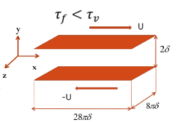
Here, represents three dimensional instantaneous fluid velocity field as function of position . denotes the instantaneous pressure field, and are the kinematic viscosity and the density of the fluid respectively. In our isothermal simulations fluid is considered to be incompressible. The flow-field is considered to be periodic along x and z direction, whereas along y-direction is bounded by walls and no-slip boundary condition is applied figure 1. The fluid flow field is solved using Direct Numerical Simulation (DNS) in a pseudo-spectral framework. Detail of the numerical scheme, interpolation method for fluid velocity at the particle location, and correction of the velocity field for the calculation of the drag on the particle has been described in detail by our earlier publications Goswami and Kumaran (2010a) and Muramulla et al. (2020).
The particle-phase is described using Newton’s equation of motion with Lagrangian particle tracking algorithm. Acceleration of the particle (p) between two successive collisions can be represented as
| (3) |
Similarly, rotational acceleration between two successive collisions, acting on the same particle is described as
| (4) |
In the above equations and denote the instantaneous translational and rotational acceleration of the ’p’th particle with translational velocity and rotational velocity . and denote the fluid phase linear and angular velocity interpolated at the particle position . is the viscous relaxation time for particle linear velocity and it is given by . For spherical particles relaxation time for angular velocity () is given by .
The inter-particle interaction is captured through standard molecular dynamics simulation algorithm (Goswami and Kumaran, 2010b, a). However, a generalized collision rule following the formulation by Lun (1991) is considered here to capture the effect of inelasticity and effect of roughness using coefficient restitution () and roughness factor () respectively.
Here, the generalised collision rule is presented briefly. Let us consider , , , be the mass, linear velocity, angular velocity, moment of inertia and diameter of the particle 1. The same symbols with a subscript 2 denote the same quantities for the second particle of the colliding pair. Vector represents the unit vector along the line joining centres from particle 1 to 2. The total relative velocity between two particles at the point of contact before and after the collision is expressed by and respectively in eq.5.
| (5) |
Where
| (6) |
and
| (7) |
For inelastic collision the coefficient of restitution is defined as,
| (8) |
For collisions between rough-particles a roughness parameter is introduced and it is defined as,
| (9) |
Roughness co-efficient can have a values between and . refers perfectly smooth collision while for indicates that the collisions are perfectly rough. In the range of spin reversal of the colliding particles takes place. To estimate the change in linear velocity and the angular velocity of the particle let us define some parameters as follows.
| (10) |
| (11) |
| (12) |
is non-dimensional moment of inertia. For a sphere having all the mass concentrated at the centre it has a value 0. For a uniform solid sphere it is . Here,
| (13) |
and
| (14) |
The change in linear and angular velocities are given by eq. 15 & eq. 16
| (15) |
| (16) |
In the present simulations, one-way coupled Direct Numerical Simulation is used because the particle volume loading () is such that there is no significant change in turbulence intensity due to the feed back force exerted by the particles Gore and Crowe (1989); Elghobashi and Truesdell (1993). All the simulations are performed using 44800 spherical particles of size 39 m which is less than the Komogorov scale Goswami and Kumaran (2010a). The investigation is conducted in the limit of high Stokes number using particle material density of .
Particle Stokes number based on integral fluid time scale is
1.7. Air at ambient condition is used as continuum fluid.
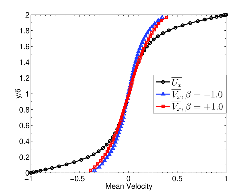
The dimension of the simulation box is where is the half-channel-width. Upper and the lower walls of the Couette move with positive and negative velocities respectively in the x-direction. The Reynolds’ Number based on half channel-width and wall-velocity is 750. The y-axis is along the cross-stream direction and z-axis indicates the span-wise or vorticity direction as shown figure 1. The number of grids used in x, y, and z directions are 340, 55, and 170 respectively. The grid resolution is 13.64 1.92 7.79 in viscous length scale. A detail description of the simulation method for smooth particle in turbulent shear flow is presented by Goswami and Kumaran (2010a). Here the statistics are presented for perfectly elastic collisions. Two limiting cases of roughness have been considered; for smooth collisions () and perfectly rough collisions ().
III Velocity and acceleration statistics for particle phase
The statistical analysis of the particle-phase translational and rotational acceleration and velocity fluctuations are presented here in the presence and absence of particle roughness. A detailed analysis of various factors governing the particle rotational acceleration distribution along with the rotational acceleration correlation and velocity auto-correlation functions is presented here. Jensen-Shannon Divergence test is applied to put the light on modelling the particle rotational acceleration distributions.
III.1 Particle statistics for smooth elastic collisions
III.1.1 Particle Acceleration Distribution
Particle acceleration distributions reflect the fluctuating statistics of the net force acting on the particles. Fluctuating acceleration originates from the fluid velocity fluctuation and also due to the particle velocity fluctuations over the local particle mean velocity as described in equation figure 17
| (17) |
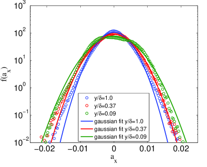
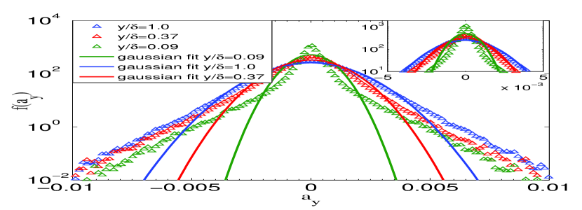
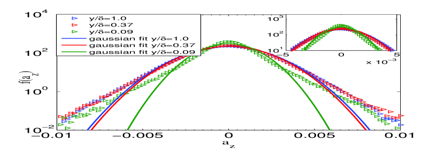
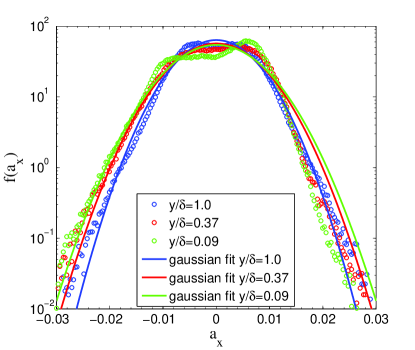
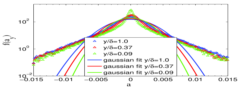
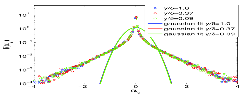
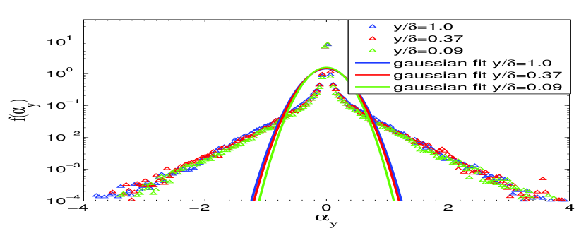
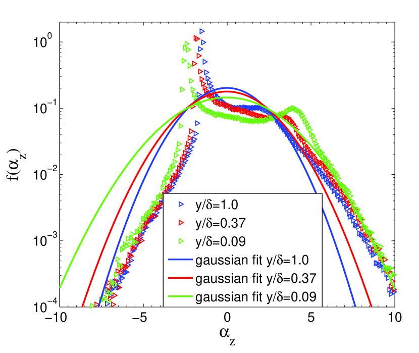
In this section, statistics of overall acceleration in three different directions at three different wall normal locations (=0.09. 0.37, and 1.0) is discussed. Hereafter we have omitted the ′ symbol in the superscript of the fluctuating quantities. Distribution functions for the streamwise, wall normal, and spanwise acceleration fluctuation are shown in figure 2 (a), (b) and (c) respectively. The variation of second, third, and fourth moments which are the mean square, Skewness, and Kurtosis along the wall normal locations are shown in figure 3. All the distribution functions have been compared with corresponding Gaussian distribution with same variance and zero mean. The traits of acceleration fluctuations are discussed here. Stream wise acceleration distribution function () can be approximated well with Gaussian distribution. Although, it deviates from the corresponding Gaussian fit at the tail of the distribution function, which is almost two orders of magnitude lower than the peak distribution (figure 2 (a)). Distribution function for wall normal () and spanwise accelerations () are shown in figures 2 (b) and (c). In both the cases distributions significantly deviate from their respective Gaussian distributions with sharper peaks and elongated exponential tails at higher values of acceleration fluctuations. deviates significantly from the Gaussian distribution at "near wall" region. Spanwise acceleration distribution also shows a similar trend of long exponential trend at the higher values of acceleration fluctuations. At the center of the Couette and intermediate locations, both the distributions and follow the Gaussian distributions more than one decade of peak distributions as shown in the insets of the figures. This is due to the fact that the second moment of the fluid velocity and particle velocity fluctuations are homogeneous at those zones.
The variance of is higher by one order of magnitude than and as shown in figure 3 (a). Streamwise mean square fluctuation is marginally higher near the wall. But for wall normal and spanwise fluctuations the variance is two times higher at the center as shown in figure 3 (a). Figure 3 (b) shows that the variation of skewness is anti-symmetric with respect to the channel-centre. is the least locally symmetric and is the most locally symmetric in nature although the values indicate that the acceleration distributions are very mildly skewed except at the center zone of the Couette. For a fluctuating variable the Skewness and excess Kurtosis is defined as:
| (18) |
| (19) |
The excess Kurtosis values for all the components of acceleration distribution functions at different wall normal locations are shown in figure 3 (c). It is observed that at the center of the Couette, tail of the distribution for all the components approximately follow Gaussian distribution. Distribution functions near the wall are far from the Gaussian for and and posses extreme outliers in the form of elongated tails as also shown in figures 2 (b) and (c).
III.1.2 Particle Velocity Distribution
In this section, distribution function and the moments of the linear velocity of the particles at different wall normal locations are reported. The distribution functions are shown in figures 4 (a) to (c) and the variation of second, third and fourth moments in the form of Mean Square, Skewness and Kurtosis along the channel-width are shown in figure 5.
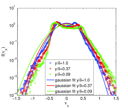
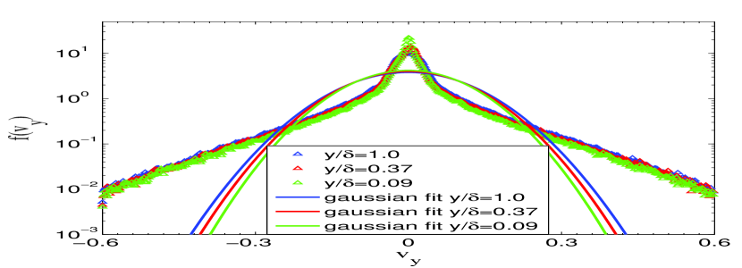
Streamwise particle velocity fluctuation can be well approximated by the Gaussian distribution except near the wall as shown in figure 4 (a). The Gaussian fits have the zero mean and same variance as that of the corresponding particle velocity distribution. In the near wall region deviates from the Gaussian distribution. At low negative velocity fluctuation the decay is slower but at higher velocity fluctuation it deacys faster that the Gaussian distribution, even though the peak distribution appears at the positive velocity fluctuation. Distribution of wall normal () and spanwise velocity field () significantly deviates from the Gaussian distribution as shown in figure 4 (b) and (c). Although there are longer exponential tails, the distribution functions can be approximated as Gaussian upto one decade of the peak frequency. Moments of the distribution functions are shown in figure 5.
The variance of is more than one order of magnitude higher than and as shown in figure 5 (a). Since local mean flow is in x direction, cross stream migration of the particles contributes to the stream wise velocity fluctuations. The variance of is higher near the walls and lower at the center of the Couette. An opposite trend is observed for and as shown in figure 5 (a). Figure 5 (b) shows that the variation of skewness is anti-symmetric with respect to the channel-centre. It is to be noted that the outward wall normal vector changes sign for both the walls. Although the magnitude shows the signature of mild asymmetry in the distribution function of wall normal velocity component, is the least locally symmetric but and is symmetric across the channel except very near the wall. Figure 3 (b) and 5 (b) show that the skewness values are of opposite signs along the channel denoting that the positive tailed particle acceleration fluctuations corresponds to negative tailed particle velocity fluctuations and vice versa. The excess Kurtosis values in figure 5 (c) shows that local can be approximated to Gaussian distribution but local and are far from the Gaussian with the existence of ’extreme outliers’ in the form of larger tails which are observed in figures 4 (a) to (c) as well.
III.1.3 Particle Rotational Acceleration Distribution
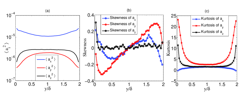
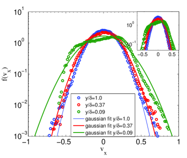
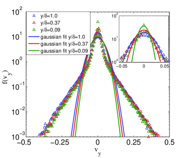
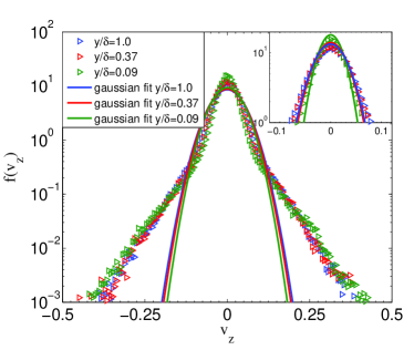
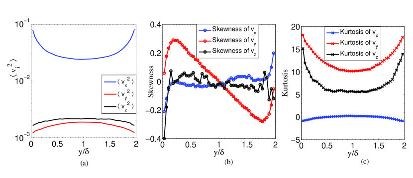
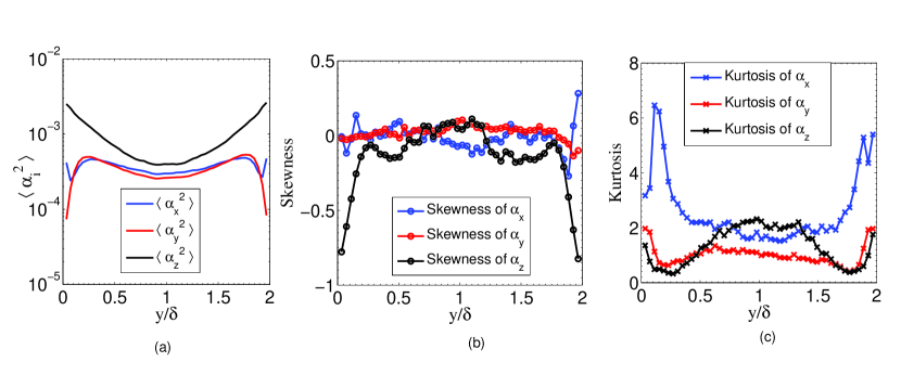
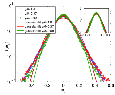
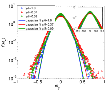
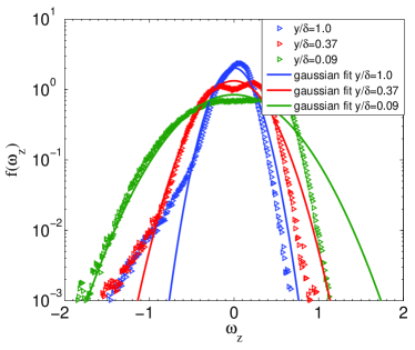
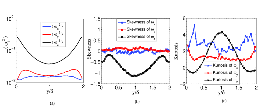
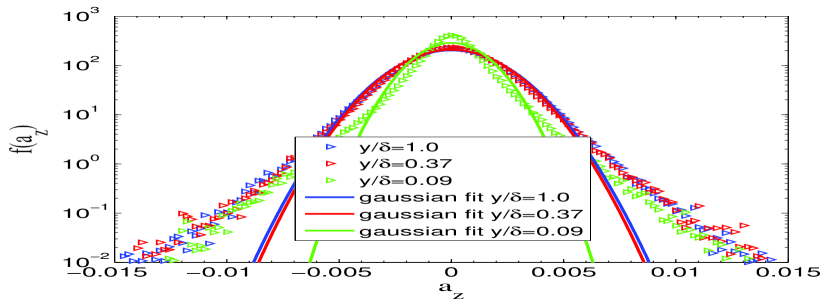
To model the dynamics of particles with surface roughness it is worth to analyze the angular acceleration and angular velocities of the particles. Here, we report the nature of rotational acceleration distribution of the particles in three directions at different wall normal locations as shown in figures 6 (a) to (c). Particle rotational acceleration statistics reflect the fluctuating statistics of the net torque acting on the particles. The variation of second, third and fourth moments in the form of Mean Square, Skewness and Kurtosis along the channel-width are shown in figure 7. The following traits of the rotational acceleration fluctuation statistics are observed.
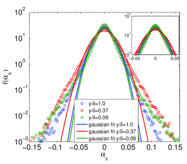
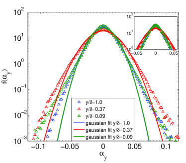
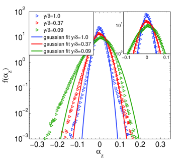
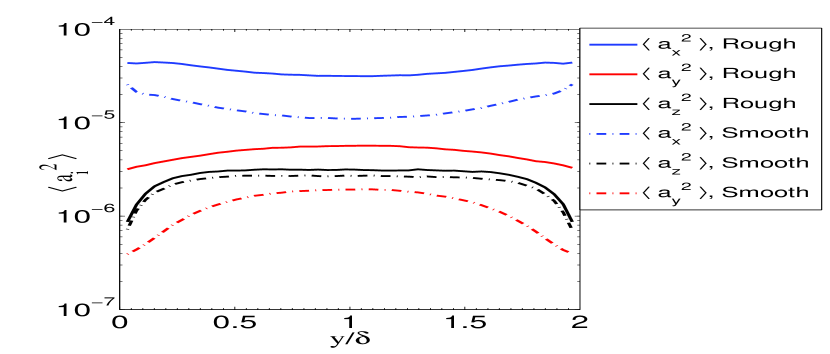
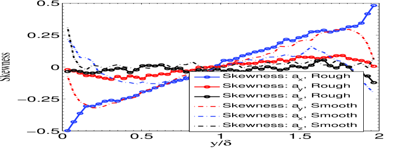
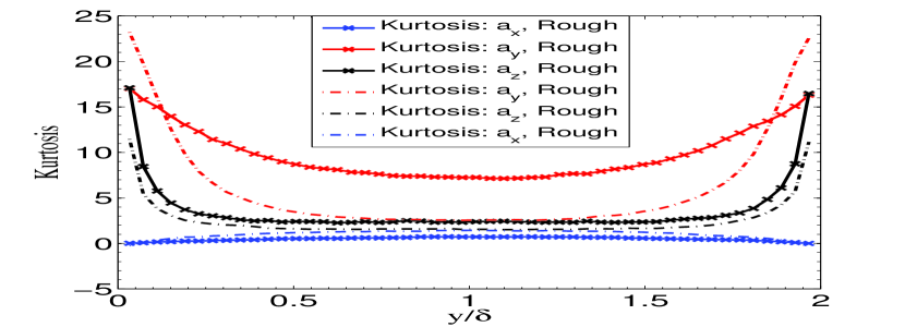
The principal component of the angular acceleration is . and deviate from their respective Gaussian fits only near the tail region with longer tails approximately exponential in nature (figures 6 (a) to (c). The tails deviate almost below two decades of the peak distribution. For both the distribution functions, an early deviation from the Gaussian distribution happens at near wall position. follows Gaussian distribution at the center of the channel where moments of the fluctuations are homogeneous. However, it deviates from the Gaussian at more than two decades below the peak frequency. This deviation happens earlier in case of distribution at the near wall region. From the plots in the insets of figures 6 (a) to (c) it is observed that upto one decade lower from the peak frequency all the components of and can be approximated by Gaussian function with the same mean and variance as that of the corresponding distribution. But for it is up to two decades. Other properties of e.g. the spread, the skewness, the flatness can be estimated from the higher moments of rotational acceleration statistics shown in figure 7. The variance of is approximately one order of magnitude higher than that of and as shown in figure 7 (a). is higher near the wall because of high fluid vorticity and decreases monotonically towards the center of the channel. In contrary and show a non-monotonic decay. and are symmetric in nature with almost zero skewness across the channel as shown in figure 7 (b). is negatively skewed near the wall with a longer negative tail observed in figure 6 (c) and also depicted by the skewness plot in figure 7 (b). Such a long tail in negative fluctuation appears due to the contribution of negative fluctuation at higher magnitude due to cross stream migration of the particle. It is worth to note that the the magnitudes of the skewness indicate that in all the cases distributions are mildly skewed. The positive excess Kurtosis values in figure 7(c) reflects deviation from corresponding normal distributions with more ’outliers’ reflected in the longer tails evident as also being reflected in figures 6 (a), (b) and (c).
III.1.4 Particle Rotational Velocity Distribution
This section describes the Particle Rotational Velocity Distribution in three different directions. All the distribution functions are plotted at three different wall normal locations in the channel as shown in figures 8 (a) to (c). Followings are the traits of fluctuating rotational velocity statistics.
Figures 8 (a), (b) show that and follow Gaussian distribution at all the wall normal locations at lower values. Deviation is observed at the tail of the distribution functions. There is a distinct deviation from the Gaussian distribution for the principal component of angular velocity . At the center of the channel there is a long tail with higher negative fluctuation, which is mainly induced by the cross stream motion of the particles from higher negative (clock wise) angular velocities. The distribution near the wall shows most probable distribution at the positive angular velocity fluctuation and also a very sharp decay at positive fluctuations. The properties of e.g. the spread, the skewness are presented by the higher moments of rotational velocity statistics shown in figure 9. is almost one order of magnitude higher than the and . Unlike , the variation of and across the channel-width is non-monotonic in nature. and are symmetric in nature with almost zero skewness across the channel as shown in figure 9 (b). shows mild negative skewness accross the channel. The positive excess Kurtosis values in figure 9(c) reflect significant deviation from corresponding normal distributions with longer tails evident in figures 8 (a) to (c). However, a small negative excess Kurtosis is observed for at the wall region (8 (c)), which corresponds to the sharper decay in the distribution at positive fluctuations.
III.2 Effect of Roughness on Particle Fluctuating Statistics
In order to understand the effect of roughness mechanistically, it is necessary to analyze the rotational and linear velocity and acceleration statistics. Therefore, this section encompasses the effect of roughness on the translational and rotational velocity and acceleration distribution functions as well as their moments in the form of Variance, Skewness and Kurtosis.
III.2.1 Particle Acceleration And Velocity Distribution
Roughness factor affect the translational acceleration and velocity distribution primarily through wall-particle collision. The average inter-particle collision times are 110 and 193 non-dimensional () units for rough and smooth particles respectively; thus indicating that in presence of roughness factor inter-particle collisions occur 1.74 times more often. The wall-particle collisions happen to be about 2.5 times more often in presence of roughness as the average wall-particle collision times are 32.25 and 80.65 units for rough and smooth particles respectively. It is observable that for both the cases wall-particle collision occur more frequently than inter-particle collision. A few pronounced effects are observed in the Particle Acceleration and Velocity fluctuations as shown in figures 11 - 18. It is to be noted that the following results are obtained at the limit of completely rough collisions i.e. . Therefore besides local fluid velocity (figure 10), particle-particle or particle-wall interactions play important role in controlling the dynamics of the particles.
The tails of an deviates slightly from the corresponding Gaussian fits at the channel center and at the intermediate location. But in case of distribution near the wall, the deviation is more prominent. Unlike smooth collisions, the high probability low magnitude zone of the fluctuations qualitatively differ from Gaussian nature with the existence of weakly bi-modal nearly symmetrical peaks (except very near the wall) at lower values of acceleration and velocity fluctuations as shown in figure 11 (a) and 15 (a). The flat distribution at the peak may originate due to increase is collision frequency and roughness induced change in tangential velocity at the contact point. Due to high frequency of collision and and high level of anisotropy in streamwise and other component of fluctuation, momentum transfer happens from streamwise to other components of fluctuations results in slowly decaying long tail in the distribution function of cross stream velocities and acceleration fluctuations as shown in figures 11 (b) , 11 (c), 15 (b), and 15 (c). The decay in is comparatively more slower than that in , which indicates that the probability of higher velocity fluctuation is more in case of , which originates because of the roughness induced momentum transfer from the moving wall. The effect of particle roughness on the second moment of acceleration and velocity fluctuations are shown in figures 14 and 18 respectively. Roughness increases the variance of velocity and acceleration distribution. There is a marginal increase in z-direction but in other two directions, variances increases significantly. The deviation of acceleration and velocity distribution form the Gaussian has been quantified in terms of skewness and kurtosis as shown in figures 14, 14, 18 and 18. A similar asymmetry is also reported in case of Granular Poiseuille Flow in presence of rough walls Vijayakumar and Alam (2007); Alam and Chikkadi (2010, 2010). The pdf deviates from Gaussian nature and the peak shifts from zero in the near wall region. In the present simulations skewness is observed at the positive fluctuation when the local mean velocity is in the negative direction and vice versa. The reason for weak bi-modality is as follows. When the particles move from the center towards the wall (we may consider the lower wall moving with -ve velocity) it induces a positive fluctuation and once it collides with the wall, due to rough collision particle will acquire more negative velocity and it will induce a negative fluctuation in the PDF. The peaks corresponds to the most probable distribution indicates the cross stream migration of the particles plays more important role in deciding the pdf of low velocity fluctuations. The trend in skewness is exactly opposite for the distribution of velocity and acceleration as shown in figures 14 and 18.


III.2.2 Particle Rotational Acceleration and Velocity Distribution
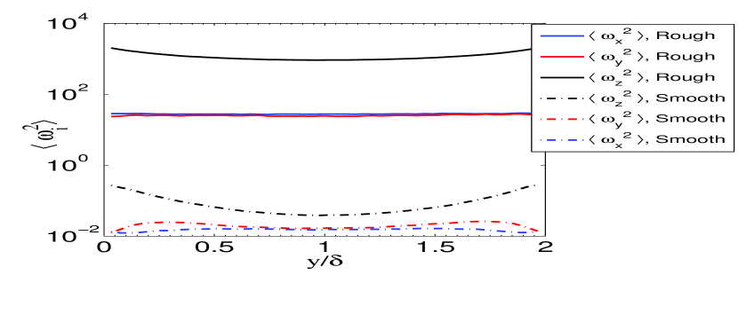
Surface roughness of the particle directly affect the angular acceleration and velocity statistics. Due to rough collisions, the mean-angular velocity gets distributed in all the directions increasing the angular acceleration and angular velocity fluctuations across the channel-width. Both the distribution functions, their skewness and flatness are presented in figures 19 to 26.
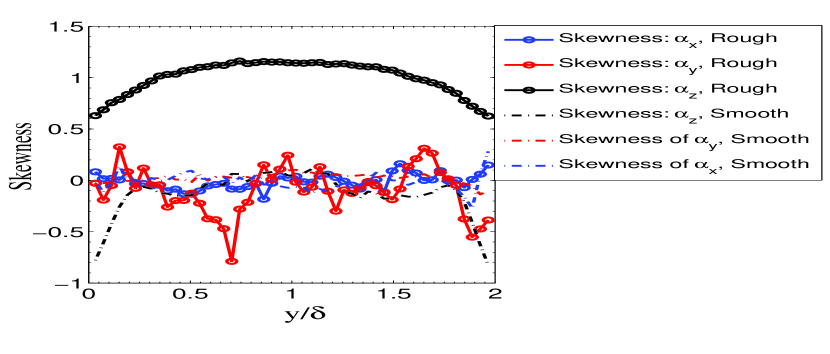
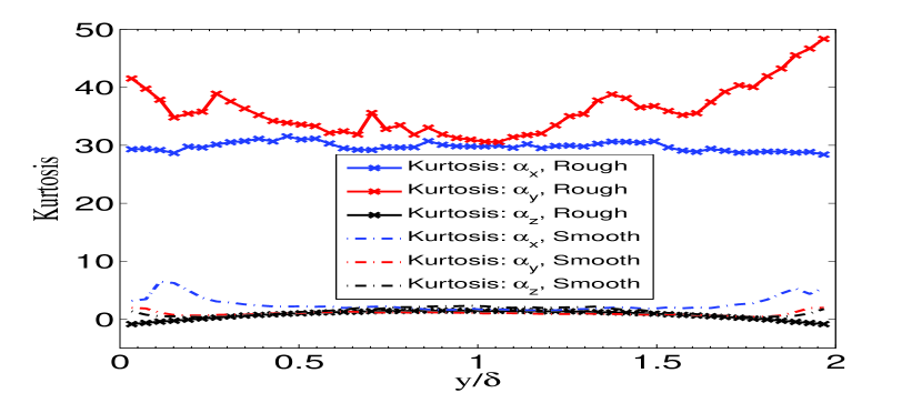
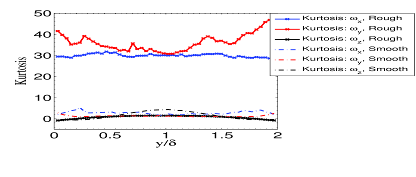
Angular acceleration and velocity distribution of stream wise and wall normal components show a significant deviation from the Gaussian distribution with slowly decaying tail for all the wall normal positions (figures 19 (a), (b), 23 (a), and (b)). Appearance of the long tail in the distribution functions is also reflected by the higher kurtosis values in figures 22 and 26.
The tails of and deviates from the corresponding Gaussian fits. Unlike smooth collisions, the high probability low magnitude zone of the fluctuations qualitatively differ from Gaussian nature. All these distributions have single sharp peaks with non-zero value accompanied with a valley about zero magnitude as shown in figures 19 (c) and 23 (c). In case of , the peaks appear at negative fluctuations with a probability almost one order of magnitude higher than the corresponding Gaussian peaks. There are also a longer positive tails at positive values of fluctuations.
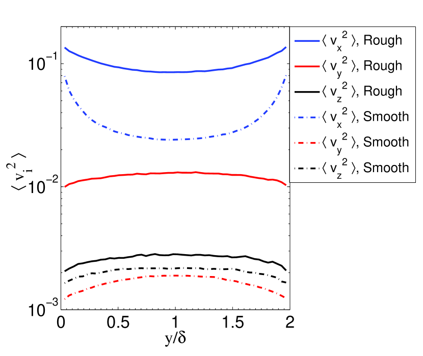
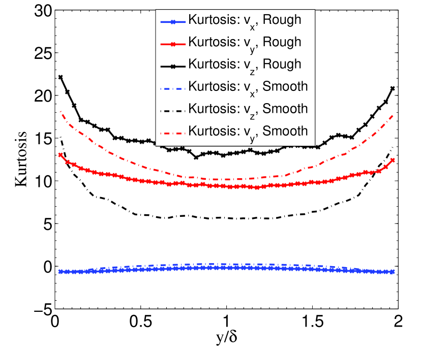
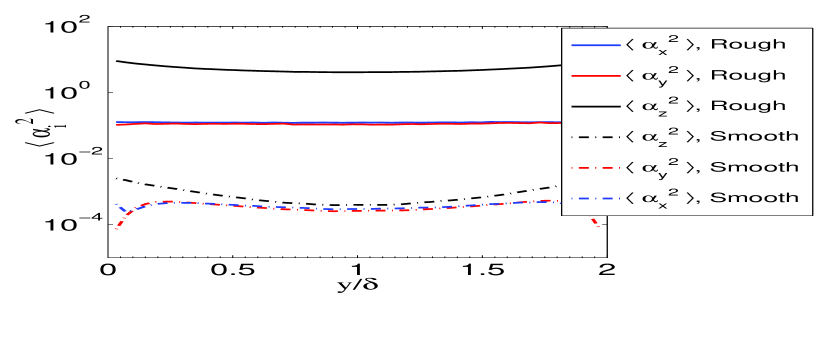
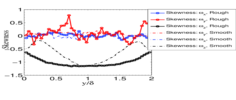
Plots of , show the peaks at positive fluctuations accompanied with longer negative tails. This is due to the fact that, in particle equation of motion net particle acceleration fluctuation and particle acceleration fluctuation originates due to particle rotational velocity fluctuation have opposite signs. Skewness of all the distribution functions are shown figures 22 and 26 at different wall normal location of the channel. Skewness is mainly observed in case of principal component of angular acceleration and angular velocity fluctuations. The increase in fluctuations due to particle surface roughness is observed through the increased variance of rotational acceleration and rotational velocities as shown in figures 22 and 26. This increase in variance for z-component is approximately four orders of magnitude but for the other two cases these are about two orders of magnitude higher than those originate from smooth particle-particle and particle-wall interactions.
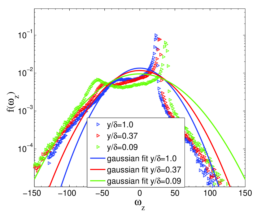
The asymmetry and sharp peak in the distribution function at the positive angular velocity fluctuation (figure 23) (c) happens as an outcome of the rough collisions between wall and the particles. Peak at the low positive fluctuation appears due to cross stream particle migration from the zone of lower angular velocity whereas negative fluctuations in the p.d.f. are mainly contributed by the particles migrates to the zone of interest after colliding with the rough wall. Distribution function for angular acceleration shows an exactly opposite trend to that of the angular velocity distribution function, which is shown in figure 19 (c). To summarize, roughness plays an important role on the variance of the particle linear and angular velocity fluctuations. Tail of the distribution functions decays more slowly in presence of rough interaction. It has been observed that in presence of roughness, frequency of inter-particle collision is 1.7 times and wall-particle collision is 2.5 times more than that occurs in the absence of roughness.
IV Modelling fluctuating torque on the particle
The particle phase equation of angular momentum can be represented by the equation 20. The net angular acceleration acting on a particle can be equated with particle rotational drag that arises due to the net slip between particle angular velocity and local fluid angular velocity, given by, . Local fluid angular velocity is computed at the particle center of mass position, . On decomposition of the rotational field variables in to a mean and a fluctuating part denoted by over-bar () and () respectively, we arrive at the expression where the fluctuating angular acceleration of the particle is expressed as a linear combination of fluid and particle rotational velocities and respectively.
| (20) |
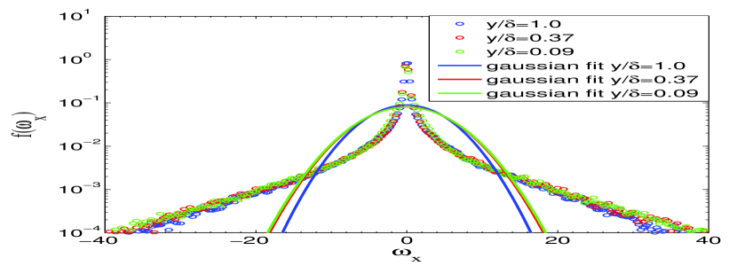
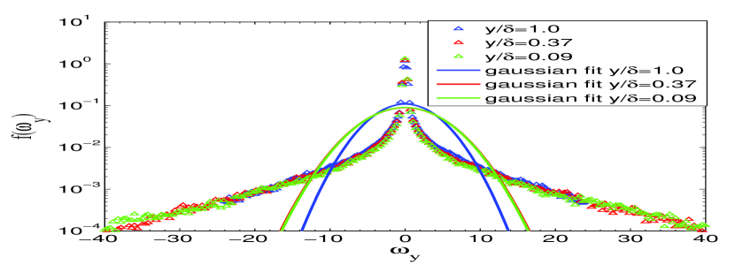
Here, represents the rotational viscous relaxation time of the particle. This section contains the comparative study of the particle rotational acceleration distribution and the particle acceleration component arising from (i) only fluctuating fluid angular velocity computed in the particle- Largrangian frame and (ii) only fluctuating particle angular velocity in three different directions at different positions of channel-width . All the results are shown in figures 27 (a) to 29 (c). In this comparison the fluid rotational acceleration computed in the fluid Eulerian grids are also shown. Hereafter, in all the figures (27 (a) to 29 (c)), we have omitted the symbol from all the fluctuating variables.
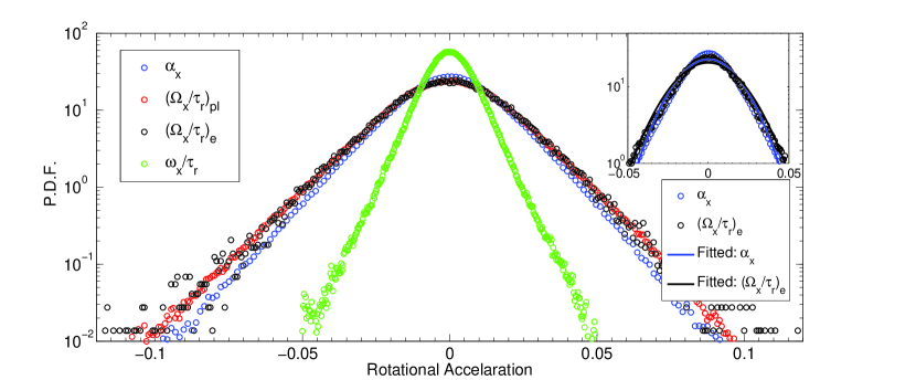
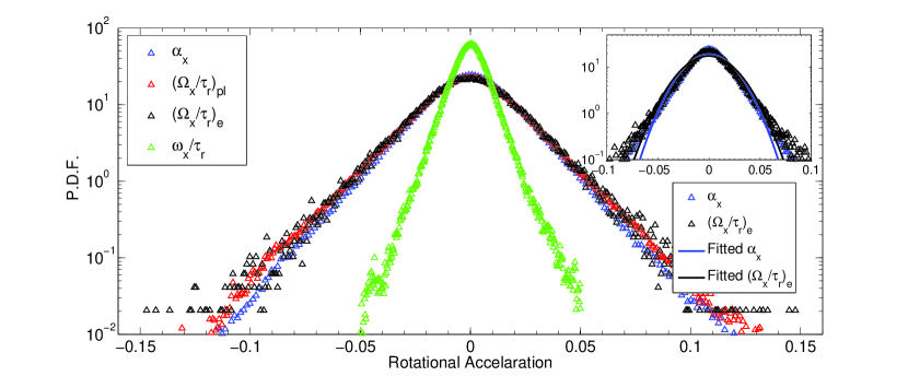
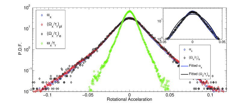
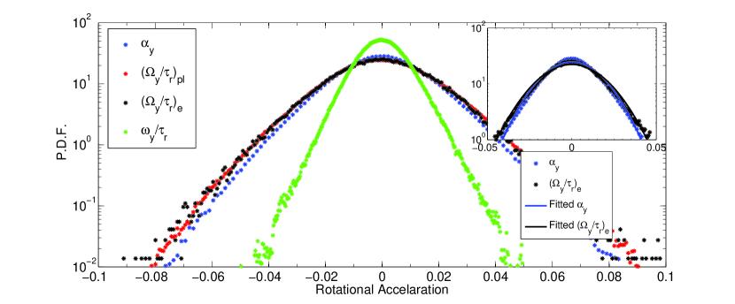
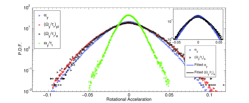
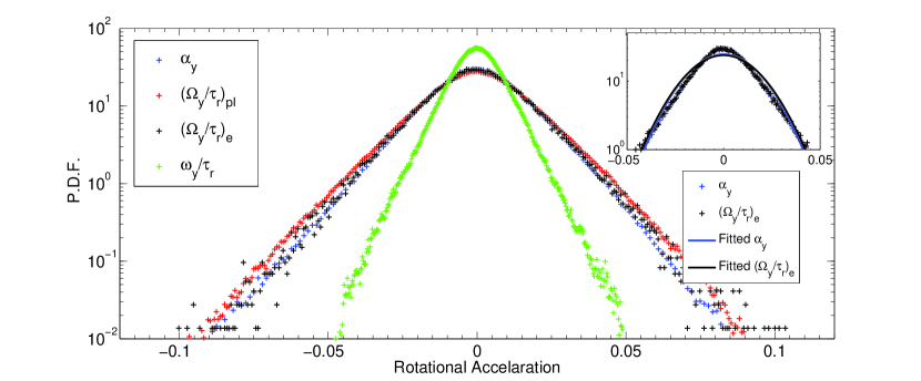
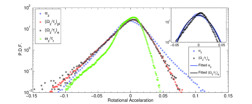
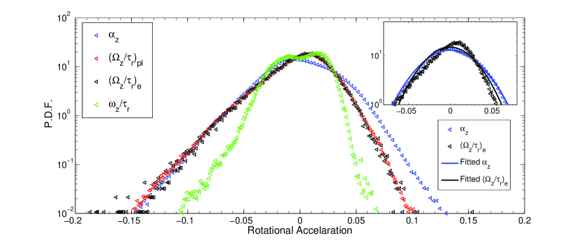
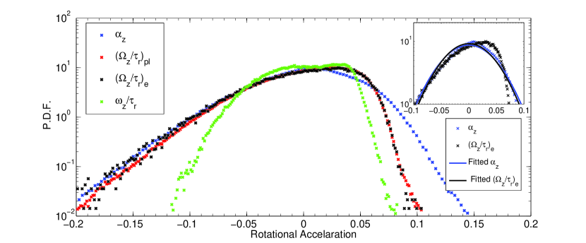
From figures 27 (a) to 29 (c) it is observed that the distribution function originates from the particle angular velocity fluctuation () does not resemble the distribution function of net particle angular acceleration fluctuation (). On the other hand, the distribution function of rotational accelerations arising out of fluid rotational velocity fluctuations computed in particle-Lagrangian frame quite resemble the net particle rotational acceleration distribution functions in all three directions. However, in case of acceleration fluctuation in z-direction, we observe a deviation at positive values of the fluctuations. In that zone pdf of particle acceleration fluctuation decays at a slower rate compared to the fluctuations originate from the fluid angular velocity fluctuations. The probability of particle acceleration originates from the fluid rotational angular velocity distribution computed in the Eulerian (fluid) Grids is similar in nature to and deviate only in the tail region. Gaussian fitting of and is performed and is shown up to one and a half to two decades lower from the peak frequency in the inset of each of the plots. The Guassian functions fit quite well for , , and . The Gaussian fits deviate marginally along the z direction especially in case of . A detailed quantification can be found in IV.1 table 4.
IV.1 The Jensen-Shannon divergence based similarity assessment
Jensen-Shannon Divergence (JSD) is a method of quantifying the similarity between two probability distribution functions. JSD is a modified symmetrized version of Kullback-Liebler (KL) divergence. The KL divergence quantifies the difference between two distribution functions and is expressed in terms of the relative Shannon-entropy of the two distributions Lin (1991).
Let and be two continuous probability distribution functions of the random variable x in probability space .
The Kullback-Liebler divergence of Q with respect to P is represented as is given by
| (21) |
Jensen-Shannon Divergence is obtained by symmetrized and smoothened KL divergence as follows:
| (22) |
where When 2 is used as the base of logarithm in KL divergence, the upper bound of JSD for two probabilities become 1. Hence, . When two distributions are identical, value becomes 0.
| Position | |||
|---|---|---|---|
| 0.09 | 0.0005 | 0.0013 | 0.1080 |
| 0.37 | 0.0016 | 0.0023 | 0.161 |
| 1.0 | 0.0034 | 0.0035 | 0.1173 |
| Position | |||
|---|---|---|---|
| 0.09 | 0.002 | 0.0005 | 0.082 |
| 0.37 | 0.005 | 0.004 | 0.1214 |
| 1.0 | 0.0038 | 0.0032 | 0.0944 |
| Position | |||
|---|---|---|---|
| 0.09 | 0.0158 | 0.0159 | 0.0674 |
| 0.37 | 0.0163 | 0.0189 | 0.0691 |
| 1.0 | 0.0105 | 0.0114 | 0.0573 |
From tables 1, 2 and 3 it is clear that the extent of similarity of to is quite lesser compared to that of and . In general is more similar to the fluid angular velocity distribution at particle Lagrangian point. But it is not feasible to assess the particle Lagrangian position during modelling the system. Therefore we have also computed JSD for the pdf of fluid angular velocity fluctuation at fluid Eulerian grid points. It is observed that the JSD values for is to . Therefore can be well approximated as .
Following the above discussion and our observation that principal component of fluid vorticity () is non-Gaussian in nature, it is tempting to perform a JSD analysis to comment on the probability of particle angular acceleration from the fluid vorticity as a Gaussian distribution function.
| Direction | Position | ||
|---|---|---|---|
| x | 0.09 | 0.0013 | 0.0191 |
| 0.37 | 0.0023 | 0.0145 | |
| 1.0 | 0.0035 | 0.0115 | |
| y | 0.09 | 0.0005 | 0.0082 |
| 0.37 | 0.0040 | 0.0068 | |
| 1.0 | 0.0032 | 0.0080 | |
| z | 0.09 | 0.0159 | 0.0072 |
| 0.37 | 0.0189 | 0.0071 | |
| 1.0 | 0.0114 | 0.0074 |
Table 4 gives a comparison of the JSD values of and its gaussian fit with respect to . It is observable that the guassian fit gives marginally lesser JSD values along z direction and greater JSD values along x direction with respect to the actual . Although overall the JSD values remain at a magnitude very near to zero O() in the interval of [0 1]. From the above plots and statistics, it is evident that can be approximated as the gaussian fit of . Hence the particle accelaration distribution function can be well approximated by a gaussian fit of the distribution function of the fluid phase angular velocity rescaled by computed in fluid-phase Eulerian grids.
IV.2 Rotational Acceleration and Velocity Correlations for Smooth Elastic Collisions
The analysis in the previous section suggests that the major constituent of the particle distribution function which originates from the fluid angular velocity can be well aproximated as a Gaussian distribution function in an Eulerian reference frame. To develop a fluid and particle phase decoupled model, it is also important to analyse the decorrelation pattern for particle angular accelaration, particle angular velocity and fluid angular velocity.
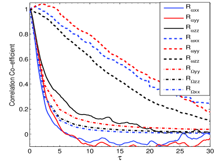
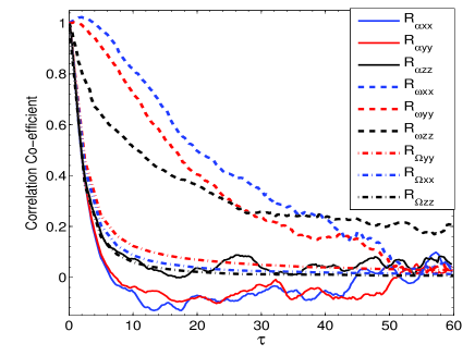
Figure 30 (a) and (b) show the temporal correlation of particle angular velocity, particle angular acceleration and fluid angular velocity at fluid Eulerian grid. It is to be noted that the last term is related to the decorrelation of particle angular acceleration which originates from fluid angular velocity and can be represented as the ratio of fluid angular velocity to the particle angular relaxation time (). In all the cases we have computed the decorrelation time by integrating the correlation coefficient up to a large time. The results are tabulated in Table5. It is observed that the particle angular acceleration decays similarly as the angular fluid velocity fluctuation; indicates that the fluctuating torque on the particle can be modeled by the particle angular acceleration fluctuation due to angular velocity fluctuation of the fluid.
| Direction | Statistics | Time-scale, y=0.6-1.0 | Time-scale, y=0.2-0.4 |
|---|---|---|---|
| x | 0.2823 | 0.6937 | |
| 24.9922 | 21.3135 | ||
| 6.6262 | 3.3033 | ||
| y | 0.8921 | 0.1774 | |
| 21.0774 | 21.573 | ||
| 11.8408 | 9.8230 | ||
| z | 3.7767 | 4.9558 | |
| 20.6116 | 14.603 | ||
| 4.5533 | 4.5524 |
Particle rotational correlations are calculated in particle-Lagrangian reference frame. So while computing the statistics in a sampling bin, particles from the bin do move out to the adjacent zones whereas particles from the neighbouring zones do move into the bin. This cross-stream movement induces noise in the correlation tails figure 30 (a) and (b). Consequently integrating over the entire domain of correlation length gives erroneous results. An approximation over the time-length cut-off is necessary. Here the rotational velocity auto-correlations are integrated over non-dimensional times and over non-dimensional times. For heavy inertial particles fluid phase rotational accelaration can be approximated as and hence the properties of covariance yields . From table 5 the following are observed:
-
•
Time-scale of particle rotational velocity de-correlation is magnitude higher than Time-scale of particle rotational acceleration de-correlation .
-
•
Fluid Eulerian rotational acceleration decorrelation time is in magnitude with respect to the particle rotational accelaration de-correlation time-scale , but quite less than particle rotational velocity decorrelation time-scale .
V Conclusion
In the present study we have analysed the translational and angular velocity and acceleration statistics of the particle phase in detail using Direct Numerical Simulation (DNS). The particles are considered to be with high Stokes number. The particle volume fraction is low such that presence of particle does not significantly modify the turbulence. Therefore one-way Direct Numerical Simulation has been performed for the present study. The inter-particle and wall-particle interactions were considered to be perfectly smooth and elastic. The fluctuating velocity, vorticity field, and mean velocity gradient of the turbulent fluid act as the primary source of particle velocity and angular velocity fluctuations rather than collisional transport. The important conclusions of the detail analysis of the velocity and acceleration distribution functions are as follows. The streamwise linear velocity fluctuation can be approximated as Gaussian distribution except very near the wall. Distribution in wall-normal and spanwise component of velocity fluctuations show exponentially decaying long tail, which originates mainly due to collisional exchange of momentum from the streamwise component. At the center of the Couette all the components of linear acceleration show a Gaussian distribution. The angular acceleration distributions are Gaussian upto two decades at the center of the Couette but asymmetry is observed near the wall. It is also observed that particle roughness plays a very important role on deciding the shape of the distribution function. From the particle equation of rotational motion, we arrive at the expression where the fluctuating angular acceleration of the particle is expressed as the ratio of a linear combination of fluctuating rotational velocities of particle () and fluid angular velocity () to the particle rotational relaxation time (for convenience all the primed superscript are dropped in the notations for fluctuations). The analysis was done using comparative study of the particle rotational acceleration distribution , with the distributions of particle acceleration component arising from (i) the fluctuating fluid angular velocity in the particle-Largrangian frame , (ii) fluctuating particle angular velocity , and (iii) the fluid rotational acceleration computed in the fluid Eulerian grids. Jensen-Shannon Divergence, which is a relative Shannon-entropy based statistic, was used to quantify the similarity of (i),(ii) and (iii) with . The rigourous statistical analysis led to the conclusion that can be well approximated by the gaussian fit of the distribution function of the ratio of fluid phase angular velocity to and computed in fluid Eulerian grids. From the sub-section IV.2 it can be substantiated that the time-scale of particle angular acceleration fluctuation and hence the net fluctuating torque is very small than that of particle rotational velocity fluctuation. Even if the particle rotational acceleration fluctuation is approximated with the ratio of Eulerian fluid phase rotational velocity to , the consequent time-scale remains substantially low. Under these circumstances the effect of fluid fluctuating torque on net particle rotational acceleration, in between two successive collisions, can be modelled as Gaussian Random White Noise. In section III.2 it is argued that the nature of distribution function changes in presence of roughness factor due to collisional re-distribution of mean translational and rotational kinetic energy along with the increase of fluctuations (mean-square values). As the change in the nature of the distribution functions is purely a collisional effect, the approximation of particle rotational acceleration, as mentioned above, in between two successive collisions, can be assumed to be unaffected by rough collisions. Hence, it is noteworthy to mention that the statistics reported in section IV and sub-section IV.2 are not required to be analysed in presence of rough collision before arriving at the applicability of the above Gaussian White-Noise approximation. The detail methodology of Langevin type modeling of the fluctuating torque due to fluid vorticity fluctuation and the resulting dynamics of the particle phase will be addressed in our future communication.
Acknowledgements.
We wish to acknowledge the financial support of SERB, DST, Government of INDIA.Data Availability Statement
The data that support the findings of this study are available from the corresponding author upon reasonable request.
References
- Soo, Ihrig Jr, and El Kouh (1960) S. Soo, H. Ihrig Jr, and A. El Kouh, “Experimental determination of statistical properties of two-phase turbulent motion,” (1960).
- Gore and Crowe (1989) R. Gore and C. T. Crowe, “Effect of particle size on modulating turbulent intensity,” International Journal of Multiphase Flow 15, 279–285 (1989).
- Elghobashi and Truesdell (1993) S. Elghobashi and G. Truesdell, “On the two-way interaction between homogeneous turbulence and dispersed solid particles. i: Turbulence modification,” Physics of Fluids A: Fluid Dynamics 5, 1790–1801 (1993).
- Louge, Mastorakos, and Jenkins (1991) M. Louge, E. Mastorakos, and J. Jenkins, “The role of particle collisions in pneumatic transport.” Journal of Fluid Mechanics 231, 345 (1991).
- Andrés and Banerjee (2019) N. Andrés and S. Banerjee, “Statistics of incompressible hydrodynamic turbulence: An alternative approach,” Physical Review Fluids 4, 024603 (2019).
- Bandi, Chumakov, and Connaughton (2009) M. Bandi, S. G. Chumakov, and C. Connaughton, “Probability distribution of power fluctuations in turbulence,” Physical Review E 79, 016309 (2009).
- Rani, Dhariwal, and Koch (2014) S. L. Rani, R. Dhariwal, and D. L. Koch, “A stochastic model for the relative motion of high stokes number particles in isotropic turbulence,” Journal of fluid mechanics 756, 870–902 (2014).
- Perrin and Jonker (2015) V. E. Perrin and H. J. Jonker, “Relative velocity distribution of inertial particles in turbulence: A numerical study,” Physical Review E 92, 043022 (2015).
- Meyer, Byron, and Variano (2013) C. R. Meyer, M. L. Byron, and E. A. Variano, “Rotational diffusion of particles in turbulence,” Limnology and Oceanography: Fluids and Environments 3, 89–102 (2013).
- Pujara et al. (2018) N. Pujara, T. B. Oehmke, A. D. Bordoloi, and E. A. Variano, “Rotations of large inertial cubes, cuboids, cones, and cylinders in turbulence,” Physical Review Fluids 3, 054605 (2018).
- Mathai et al. (2016) V. Mathai, M. W. Neut, E. P. van der Poel, and C. Sun, “Translational and rotational dynamics of a large buoyant sphere in turbulence,” Experiments in fluids 57, 51 (2016).
- Lamballais, Lesieur, and Métais (1997) E. Lamballais, M. Lesieur, and O. Métais, “Probability distribution functions and coherent structures in a turbulent channel,” Physical Review E 56, 6761 (1997).
- Gustavsson and Mehlig (2011) K. Gustavsson and B. Mehlig, “Distribution of relative velocities in turbulent aerosols,” Physical Review E 84, 045304 (2011).
- Gustavsson and Mehlig (2014) K. Gustavsson and B. Mehlig, “Relative velocities of inertial particles in turbulent aerosols,” Journal of Turbulence 15, 34–69 (2014).
- Bhatnagar et al. (2018) A. Bhatnagar, K. Gustavsson, B. Mehlig, and D. Mitra, “Relative velocities in bidisperse turbulent aerosols: Simulations and theory,” Physical Review E 98, 063107 (2018).
- Goswami and Kumaran (2010a) P. S. Goswami and V. Kumaran, “Particle dynamics in a turbulent particle–gas suspension at high stokes number. part 1. velocity and acceleration distributions,” Journal of Fluid Mechanics 646, 59–90 (2010a).
- Andersson, Zhao, and Barri (2012) H. I. Andersson, L. Zhao, and M. Barri, “Torque-coupling and particle–turbulence interactions,” Journal of Fluid Mechanics 696, 319–329 (2012).
- Marchioli and Soldati (2013) C. Marchioli and A. Soldati, “Rotation statistics of fibers in wall shear turbulence,” Acta Mechanica 224, 2311–2329 (2013).
- Muramulla et al. (2020) P. Muramulla, A. Tyagi, P. Goswami, and V. Kumaran, “Disruption of turbulence due to particle loading in a dilute gas–particle suspension,” Journal of Fluid Mechanics 889 (2020).
- Goswami and Kumaran (2010b) P. S. Goswami and V. Kumaran, “Particle dynamics in a turbulent particle–gas suspension at high stokes number. part 2. the fluctuating-force model,” Journal of Fluid Mechanics 646, 91–125 (2010b).
- Lun (1991) C. Lun, “Kinetic theory for granular flow of dense, slightly inelastic, slightly rough spheres,” Journal of fluid mechanics 233, 539–559 (1991).
- Vijayakumar and Alam (2007) K. Vijayakumar and M. Alam, “Velocity distribution and the effect of wall roughness in granular poiseuille flow,” Physical Review E 75, 051306 (2007).
- Alam and Chikkadi (2010) M. Alam and V. Chikkadi, “Velocity distribution function and correlations in a granular poiseuille flow,” Journal of fluid mechanics 653, 175 (2010).
- Lin (1991) J. Lin, “Divergence measures based on the shannon entropy,” IEEE Transactions on Information theory 37, 145–151 (1991).