Points2Polygons: Context-Based Segmentation from Weak Labels Using Adversarial Networks

Abstract

In applied image segmentation tasks, the ability to provide numerous and precise labels for training is paramount to the accuracy of the model at inference time. However, this overhead is often neglected, and recently proposed segmentation architectures rely heavily on the availability and fidelity of ground truth labels to achieve state-of-the-art accuracies. Failure to acknowledge the difficulty in creating adequate ground truths can lead to an over-reliance on pre-trained models or a lack of adoption in real-world applications. We introduce Points2Polygons (P2P), a model which makes use of contextual metric learning techniques that directly addresses this problem. Points2Polygons performs well against existing fully-supervised segmentation baselines with limited training data, despite using lightweight segmentation models (U-Net with a ResNet18 backbone) and having access to only weak labels in the form of object centroids and no pre-training. We demonstrate this on several different small but non-trivial datasets. We show that metric learning using contextual data provides key insights for self-supervised tasks in general, and allow segmentation models to easily generalize across traditionally label-intensive domains in computer vision.

1 Introduction

Segmentation tasks based on remotely-sensed imagery rely heavily on the availability of good quality semantic or polygon labels to be useful [28, 31]. Specifically, [1] notes that the performance of ConvNets for segmentation tasks is largely dependent on the amount of time spent creating training labels. These tasks can be as simple as instance counting [19, 21, 23, 30] or object identification [5, 13]. However, in practice these labels tend not to be readily available outside of established tasks such as building footprint extraction or vehicle detection, so it is often necessary to spend significant manual effort to digitize these polygons [28]. This drastically increases the cost to build segmentation models for practical applications, and presents a major barrier for smaller organizations.

Several approaches have been proposed in response to this issue such as weak-label learning [2, 16, 24, 28] and self-supervision via a contrastive objective in Siamese or Triplet networks [4, 10, 15, 17]. However, these approaches come with their own problems. Models based on weak labels for instance are challenging to evaluate since ground truth polygons are not necessarily meaningful labels. In the case of aerial imagery, a model which fixates on salient features of an object such as a chimney or a wind shield should not be penalized for having a non-intuitive interpretation of what best defines a building or a vehicle.

This paper contributes a novel approach to semantic segmentation with weak labels by incorporating constraints in the segmentation model $S$ through an adversarial objective, consisting of an object localization discriminator $D_{1}$ and a contextual discriminator $D_{2}$.

In our framework, $D_{1}$ discriminates between the true image $I_{R}$ and a fake image $I_{F_{1}}$, where $I_{F_{1}}$ is a spatially similar sample in the training set with the positive object superimposed to it. By treating the segmentation model as a generator, and implementing an additional discriminator, we propagate learnable gradients back to the generator. This allows the segmentation model to produce masks which when used to superimpose the original image into neighboring contexts, produce believable “generated” images. The full formulation of the discriminator and the superimpose function $f$ is discussed in Section 3.1. $D_{2}$ is an additional contextual discriminator which we introduce in order to constrain artifacts that arise from having only one discriminator.

We show that this method produces high quality segmentations without having to consider imagery gradients and uses only buffered object polygon centroids as inputs. The major contribution of this paper is a new form of semi-supervised segmentation model that can be applied to segment objects using weak labels, such as those provided by manual annotation or object detection models which only provide bounding boxes. Future extensions of this work will address the localization task, providing end-to-end instance segmentation from weak labels and low requirements for the number of annotations to reach acceptable performance.

2 Related Work

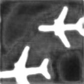
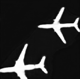
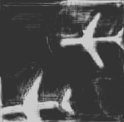
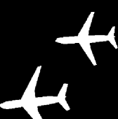
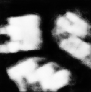
(a)	(b)	(c)	(d)	(e)	(f)	(g)

Figure 1: Predicted segmentation masks from the Aircraft and Woolsey datasets using fully-supervised UNet models with ResNet backbones (c-e) and our semi-supervised P2P model (f). All generated masks come from training with Dice loss, besides (e), which is trained with cross entropy loss for comparison. (a) Input image to each model. (b) Pseudo label $\tilde{y}$ used to train P2P. (c) Output from a UNet-101 baseline model. (d) Output from UNet-50. (e) Output from UNet-50 trained with cross-entropy. (f) Output from P2P (ours). (g) Ground Truth labels.

Points2Polygons shares ideas in common with four general types of segmentation models which we will discuss here:

Footprint extraction models

We make a reference to building footprint extraction models because these models aim to extract (either via semantic or instance segmentation) complex geometries that come from a much more complex distribution space - in terms of shape and texture variance - than features such as vehicles or trees [3, 6, 32]. Building footprints are also a class of features which are conditionally dependent on contextual information; a building is much more likely to be found in a suburban context next to trees or driveways as opposed to in the desert.

Existing approaches however rely heavily on segmentation labels [6, 32] and primarily focus on improving the accuracy from a supervised learning approach given large amounts of training data, such as in the SpaceNet [11] and WHU [29] datasets. This is unfortunately not readily available for many worthwhile segmentation tasks such as well pad extraction for localizing new fracking operations or airplane detection for civil and remote sensing applications.

Semi-supervised or unsupervised methods

Other methods such as [1, 2, 16, 24, 28] and [9] attempt to address the scarcity of existing ground truth labels by adopting a semi-supervised or unsupervised approach. These include methods which attempt to perform segmentation based on a single datapoint as demonstrated in [28]. However approaches such as these only factor in low-frequency information and are designed for landcover classification. Laradji et al. [16] utilizes point-based pseudo labels to segment objects of interest in imagery using a network with a localization branch and an embedding branch to generate full segmentation masks. While similar in nature to P2P, [16] optimizes a squared exponential distance metric between same-class pixels in embedding space to generate segmentation masks, whereas P2P frames the segmentation task as a simple image-to-image translation problem with localization constraints enforced by an adversarial objective. Our approach thus circumvents the need for pair-wise calculations from a similarity function with the additional benefit of a separately tunable constraint.

[7] attempts to solve segmentation problems in a completely unsupervised setting using an adversarial architecture to segment regions that can be clipped and redrawn using a generator network such that the generated images is aligned with the original. P2P goes further by using easy-to-obtain supervised labels that consist of points within individual instances.

An alternate approach to weak supervision for segmentation is to utilize image-level class labels in conjunction with class attention maps [2, 22]. Besides the low labeling cost, the benefit of this approach is that the class boundary for the object of interest is informed by contextual information in the rest of the image, in contrast to pixel-level supervision, where the model is encouraged to learn shape and color cues in the object of interest. P2P incorporates image-level information by learning characteristics of an object’s context via a second contextual discriminator, $D_{2}$, as described in Section 3.1.

Adversarial methods

One of the primary difficulties of learning segmentation from weak labels is that it is difficult to evaluate the quality of the segmentation model in the absence of ground-truth polygons. Traditional methods tackle this challenge by introducing priors or domain-specific constraints, such as in superpixel-based models [8, 12, 14, 26]. However this approach is difficult to generalize to cases where the landscape changes or in the presence of covariate shift introduced via a new dataset.

In these cases, it may be necessary to adjust model hyperparameters, such as is commonly done in experiments with production-level segmentation pipelines in order to compensate for these new domains which in itself can be very time-intensive.

We draw inspiration from works that leverage Generative Adversarial Networks (GANs) which aim to introduce a self-imposed learning objective via a discriminator $D$ which models and attempts to delineate the difference in distribution between a real and fake input set. In particular, Luc et al. [20] uses an adversarial network to enforce higher-order consistency in the segmentation model such that shape and size of label regions are considered, while Souly et al. [27] use GANs to create additional training data.

This is a form of self-supervision which we are able to incorporate into P2P. By introducing discriminators, we get past the need to impose strong human priors and instead allow the model to determine whether or not the segmentation output is “realistic”. In effect, our optimization objective enforces contextual consistency through a $\min\max$ formulation. We additionally modify the vanilla GAN objective in order to prevent high model bias, which we outline under Contextual Similarity in Section 3.2

3 Methodology

Figure 2: Our modified adversarial objective. Our segmentation model $S$ takes in pseudo label $\tilde{y}$ and $I_{R}$ and returns a predicted segmentation mask $\hat{y}$, which is then used to generate fake images $I_{F_{1}}$ and $I_{F_{2}}$, which are used to train the discriminators $D_{1}$ and $D_{2}$. See Section 3.1 for more details on this procedure.

3.1 Adversarial Objective

This is the vanilla GAN objective:

$$\min_{G}\max_{D}\operatorname{\mathcal{L}}(G,D)=\operatorname{\mathbb{E}}_{x\sim p_{data}}[\log D(x)]+\operatorname{\mathbb{E}}_{z\sim p(z)}[\log(1-D(G(z)))]$$ (1)

We modify the vanilla GAN objective by introducing an additional discriminator which forces the generator to include features which contribute more to the object of interest than its background. P2P uses an adversarial objective using two discriminators, $D_{1}$ and $D_{2}$. The first discriminator $D_{1}$, discriminates between the real input $I_{R}$ and a fake variant of the input, $I_{F_{1}}$, which consists of the object of interest superimposed to a spatially similar training sample, $I_{ctx}$. The second discriminator $D_{2}$ uses a similar approach, but with a different fake image, $I_{F_{2}}$. For this discriminator, the negative area around the object of interest is used to create the fake image.

Fake images used in our GAN formulation are generated by combining the predicted segmentation mask $\hat{y}$ with our original image $I_{R}$ and context image $I_{ctx}$ through a process equivalent to alpha blending [25].

Formally, the process to generate a fake sample is

$$f(I,I_{ctx},y)=y\odot I+y^{c}\odot I_{ctx}$$ (2)

where $I,I_{ctx}\in T$, $\odot$ is the Hadamard product and $y$ is a segmentation mask. Both $I$ and $I_{ctx}$ are samples from the training dataset $T$, where $I_{ctx}$ is found by iterating through adjacent tiles to $I$ until a tile without a training label appears, and is chosen to be $I_{ctx}$. Figure 3 describes the procedure to find $I_{ctx}$ in more detail.

In P2P’s case, $I\equiv I_{R}$ is the "real" input image fed into the discriminators and $\hat{y}$ is used in place of $y$ for generating $I_{F_{1}}$, while $\hat{y}^{c}=(1-\hat{y})$ is used for generating $I_{F_{2}}$. Therefore, the fake images are generated using

$$I_{F_{1}} =f(I_{R},I_{ctx},\hat{y})=\hat{y}\odot I_{R}+\hat{y}^{c}\odot I_{ctx}$$ (3)

$$I_{F_{2}} =f(I_{R},I_{ctx},\hat{y}^{c})=\hat{y}^{c}\odot I_{R}+\hat{y}\odot I_{ctx}$$ (4)

The operation $f(\cdot)$ used to generate the fake examples can be thought of as a superimpose operation that uses the predicted segmentation mask to crop the object of interest (or its background) and paste it in a nearby training sample.

Given the above definitions for our real and fake images for $D_{1}$ and $D_{2}$, we arrive at the following objective:

$$\min_{G}\max_{D}\operatorname{\mathcal{L}}(G,D) =\min_{G}\max_{D}\operatorname{\mathbb{E}}_{\chi\sim p_{data}}(2\log(1-D_{1}(G_{1}))+2\log(1-D_{2}(G_{2}))$$

$$+\log(D_{1}(I_{R}))+\log(D_{2}(I_{ctx}))+\operatorname{\mathcal{L}}_{loc})$$ (5)

where $\chi=(I_{R},I_{ctx})$, $D=(D_{1},D_{2})$ and $G=(G_{1},G_{2})$, $G_{1}=f(\hat{y},I_{R},I_{ctx})$, and $G_{2}=f(\hat{y}^{c},I_{R},I_{ctx})$. Note that $G_{1}$ and $G_{2}$ share weights; they are both functions of the segmentation model $S(I_{R},\tilde{y})=\hat{y}$, although $G_{2}$ uses the complement of $\hat{y}$, namely $\hat{y}^{c}$, to generate fake samples.

The loss function $\operatorname{\mathcal{L}}(G,D)$ for P2P is the sum of $D_{1}$ and $D_{2}$’s binary cross entropy loss, a generator loss $\operatorname{\mathcal{L}}_{G}$, and a localization loss $\operatorname{\mathcal{L}}_{loc}=\min(\tilde{y}\cdot\log(\hat{y})+(1-\tilde{y})\cdot\log(1-\hat{y}),\rho)$ that is included in $\operatorname{\mathcal{L}}_{G}$. The localization loss term is a thresholded version of binary cross entropy, where $\rho$ is the threshold parameter that controls the amount of influence that $\operatorname{\mathcal{L}}_{loc}$ has on the overall loss function. This parameter is chosen with a hyperparameter search, specifically ASHA [18]. For more details on how the objective function is derived, please see the Appendix.

3.2 Contexts

Figure 3: Contexts (blue tiles) are discovered by expanding out from an origin tile, denoted in violet. Origin tiles are tiles containing positive samples (orange) which are indexed during preprocessing then sampled at random during training. We first index the surrounding 8 tiles from the origin. Positive tiles $I_{R}$ are denoted in orange while contexts $I_{ctx}$ (negative tiles) are denoted in blue. If the number of contexts do not meet the minimum context number, we continuously expand the search space until a sufficient number of positive tiles are met.

To support the generator in producing realistic fake outputs without being overpowered by the discriminator, we need to place these outputs in contexts that are realistic and do not expose information which might signal to the discriminator that these outputs are fake. As an example we do not want to superimpose objects against a purely black or noisy background. However we do want to place these buildings in a suburban neighborhood with trees and roads. We define the term context as an image tile in close proximity to a tile in question which also does not contain a positive sample.

P2P requires each context to be extracted from a positive tile’s spatial neighborhood to maintain semantic similarity with the rest of the inputs. We provide users the flexibility to choose the number of contexts that are aggregated into each batch at training time. This ensures a diverse selection of background characteristics for the superimpose function. To facilitate dynamic tile fetching during training without heavy computational overheads, we map each positive tile to its neighboring contexts during a preprocessing step (see Figure 3). The output of this step is a dictionary that maps each positive tile to a set number of neighboring contexts which is then used by P2P to quickly access these tiles for training.

3.3 Object Localization

Since the discriminators do not actually care about whether or not the extracted features exhibit sufficient localization behavior, only that these outputs look “realistic”, we reinforce the generator with a localization objective. This objective makes use of the input point labels, which we term pseudo labels, and creates a buffer around these points against which the output segmentation masks are evaluated. In particular, we try to minimize the ratio between the amount of positive pixels in the output segmentation mask and this buffer. We also set a minimum threshold to how low this ratio can go to prevent the model from overweighting the localization objective.

4 Implementation

Figure 4: The general procedure for generating fake images from an input sample $I_{R}$ and predicted segmentation mask $\hat{y}$. The GAN training procedure is designed to generate segmentation masks $\hat{y}$ that create believable “fake” examples.

In preprocessing, we divide up the input rasters into multiple image chips. For each positive image chip, we search its 8 neighboring contexts in order to index any negative chips (chips which do not contain positive samples). If these cannot be found in the immediate contexts, we expand our search to the next 16 contexts and the next 32 contexts etc. For every positive chip we store a number of its negative neighbors (up to $k$ neighbors) in the context dictionary.

In the training step, we jointly train the segmentation model (generator) along with two discriminators. We sample a batch of positive chips and feed them to the generator to produce output masks. These are then used to “transplant” the positive features from the original positive context into neighboring negative contexts to produce fake positives. Both the real and fake positives are fed into $D_{1}$ to evaluate the positive transplants.

To prevent the generator from overpowering the discriminator using salient but ill-segmented features, we also produce negative contexts. The real negative contexts are the original neighbors while the fake negative contexts are created by transplanting features from the positive context to its neighboring negatives using the inverse of the output mask. These are fed to $D_{2}$.

Finally at inference time, we simply extract the raw outputs of the generator.

5 Experiments

Table 1: Fully-supervised benchmark comparison.

	Dice				Jaccard				Recall				Precision
Model	Well Pads	Airplanes	Woolsey	SpaceNet	Well Pads	Airplanes	Woolsey	SpaceNet	Well Pads	Airplanes	Woolsey	SpaceNet	Well Pads	Airplanes	Woolsey	SpaceNet
UNet-50	$0.33$	$0.65$	$0.46$	$0.47$	$0.20$	$0.49$	$0.31$	$0.31$	1.00	1.00	0.99	1.00	$0.20$	$0.49$	$0.31$	$0.31$
UNet-101	$0.21$	$0.46$	$0.57$	$0.47$	$0.12$	$0.30$	$0.41$	$0.32$	1.00	1.00	$0.85$	1.00	$0.12$	$0.30$	$0.44$	$0.32$
UNet-50 (CE)	0.80	0.90	0.81	0.90	0.68	0.82	0.70	0.82	$0.90$	$0.86$	$0.80$	$0.89$	0.75	0.94	0.85	0.92
P2P (ours)	$0.65$	$0.64$	$0.66$	$0.62$	$0.49$	$0.48$	$0.51$	$0.46$	$0.93$	$0.67$	$0.74$	$0.60$	$0.52$	$0.64$	$0.64$	$0.68$

5.1 Datasets

In our experiments, we make use of five datasets to train P2P and assess its performance. This includes two small datasets for well pads and airplanes as described in the Appendix, and one medium dataset for building footprint extraction which we sourced from USAA. We also train and benchmark our model against the SpaceNet Challenge AOI2 Las Vegas dataset [11]. Additionally, as part of our ablative studies we also create a smaller version of this dataset which we name Vegas Lite.

Well pad dataset

We construct a well pad dataset using NAIP: Natural Color imagery at 1.5m resolution. This dataset is created using ArcGIS Pro and contains 9 training rasters and 1 testing raster. There are 2909 training samples and 426 testing samples, which makes this a small-to-medium sized dataset. The labels are bounding geometries of visible well pads, which contain both active and disused examples.

Airplane dataset

We construct an airplane dataset using NAIP: Natural Color imagery at 0.5m resolution. This dataset is created using ArcGIS Pro and contains 2 training rasters and 1 testing raster. Given there are 335 training samples and 40 testing samples, this constitutes a small dataset and what can be realistically expected in a real-world proof-of-concept application. The labels incorporate a variety of plane sizes from 3 locations in the United States: Southern California Logistics Airport, Roswell International Air Center and Phoenix Goodyear Airport.

Woolsey Fire dataset

We make use of the DataWing imagery from USAA that was captured after the 2018 Woolsey Fires for damage assessment. These are 0.3m resolution rasters with 8682 training samples distributed across 6 training rasters and 572 samples on 1 testing raster. This is a medium sized dataset and contains a large number of negative samples (of damaged houses) in a variety of terrains.

SpaceNet Challenge: Las Vegas dataset

In order to benchmark our model against popular datasets for remote sensing, we make use of the SpaceNet Las Vegas (AOI2) dataset [11]. Both training and testing sets are publicly available however the testing set does not contain ground truth geometries. We therefore further split the training set into 2905 image tiles for training (tiles numbered 1325 and above) and 712 image tiles for testing (tiles up to, but not including, 1325).

Vegas Lite dataset

We further reduce the size of the Las Vegas dataset in order to perform ablative tests on a smaller set of samples. This we call the Vegas Lite dataset and is simply the full Las Vegas Dataset without any tiles numbered 3000 upwards in the training set and 500 upwards in the testing set. This dataset contains 970 tiles in the training set and 268 tiles in the testing set. These are roughly 33% and 38% the size of the original training and testing sets respectively, assuming samples are equally distributed across tiles.

We use the Vegas Lite dataset to understand the importance of contextual similarity between positive and negative chips. We do so by introducing a series of negative rasters with varying contextual similarities in our ablative tests.

5.2 Performance Study

We evaluate our model based on several real-world feature segmentation tasks in order show the efficacy of our proposed approach.

P2P vs Baseline Comparison

We compare P2P which uses weak labels $\tilde{y}$ against 3 fully supervised segmentation models which make use of ground truth polygon labels $y$. Among baselines trained with Dice loss, we find that UNet-50 produces the best results on all except the well pads dataset, where UNet-18 performs the best out of the baseline models. In the case of well pad extraction, an increase in the number of parameters in the model results in lower performance, suggesting that a low-complexity problem such as well pad extraction could be over-parameterized in this approach. A considerable improvement is made to the performance of baseline models with full labels when trained with cross-entropy loss, which produces better learnable gradients for these datasets. A survey of the visual outputs show that these baselines generally produce segmentation masks that are significantly larger than the object outlines which is not the case for P2P. We further clarify that these P2P results consider the optimal localization guidance parameters, however it is not difficult to select a uniform guidance parameter that would outperform all baselines (7000 for example).

5.3 Ablative Tests

Negative Discriminator

We explore the impact of a second negative discriminator on testing accuracy through all 4 datasets. We define this second discriminator $D_{2}$ as a UNet-50 (same as $D_{1}$) binary classifier which predicts the probability that its input comes from the distribution of real negatives. Negative samples associated with a specific positive sample are drawn from the positive sample’s neighboring contexts. This is done during preprocessing as discussed in Section 3.4. We then employ the context shift function $f$ to superimpose the positive sample $I_{R}$ to its context $I_{ctx}$ using the inverse of the labels. This creates our fake negative sample $I_{F_{2}}$, which we jointly feed to $D_{2}$ along with the real context $I_{ctx}$.

In experimentation, we find that implementing $D_{2}$ significantly improves model performance across all but one of the datasets. In the well pads dataset, we find that introducing $D_{2}$ incurs a small performance cost. This is possibly due to the simple nature of the segmentation task where having additional tunable parameters potentially lead to model overfitting.

By observing the quantitative and visual outputs we identify that the lack of $D_{2}$ generally leads to segmentation masks with much lower precision and higher recall.

Table 2: Negative Discriminator $D_{2}$ ablative study.

	Dice			Jaccard			Recall			Precision
Model	Well Pads	Airplanes	Woolsey	Well Pads	Airplanes	Woolsey	Well Pads	Airplanes	Woolsey	Well Pads	Airplanes	Woolsey
P2P w/o $D_{2}$	0.67	$0.23$	$0.43$	0.51	$0.13$	$0.28$	$0.92$	0.96	0.90	0.54	$0.13$	$0.30$
P2P w/ $D_{2}$	$0.65$	0.64	0.66	$0.49$	0.48	0.51	0.93	$0.67$	$0.74$	$0.52$	0.64	0.64

Localization Guidance

We show that a purely unsupervised approach without any guidance on object localization does not produce good results in practice. In order to guide the model during training, we create a buffer around object centroids at training time and incur a penalty on the generator whenever predicted masks do not cover these buffered pixels. We then threshold this loss to prevent this localization loss from overwhelming the generator. A failure case would be the model treating the buffered centroids as the ground truth labels under a fully supervised objective. By thresholding, we ensure that the model is only concerned with localization at a rough scale.

To qualify the optimal buffer size for a variety of datasets we trained P2P using a variety of preset buffer sizes. This is a variable we term centroid size multiplier (csm). The exact formulation for localization loss and additional visual results can be found in the Appendix.

We also recognize that a shortfall of this method is that it is less suitable for detecting objects that do not share the same size. This is of lesser concern for remote sensing use cases but should be taken into consideration when applying this model to general-purpose segmentation tasks.

Table 3: Localization Guidance ablative study for various csm values.

	Dice			Jaccard			Recall			Precision
Model (csm)	Well Pads	Airplanes	Woolsey	Well Pads	Airplanes	Woolsey	Well Pads	Airplanes	Woolsey	Well Pads	Airplanes	Woolsey
P2P ($6000$)	$0.27$	$0.15$	$0.04$	$0.16$	$0.09$	$0.02$	$0.72$	$0.17$	$0.02$	$0.17$	$0.18$	$0.17$
P2P ($7000$)	$0.55$	0.64	0.66	$0.39$	0.48	0.51	0.87	$0.67$	$0.74$	$0.42$	$0.64$	$0.64$
P2P ($8000$)	$0.64$	$0.54$	$0.54$	$0.48$	$0.38$	$0.38$	$0.84$	$0.78$	$0.49$	$0.54$	$0.42$	$0.64$
P2P ($9000$)	$0.07$	$0.56$	$0.64$	0.50	$0.39$	$0.48$	$0.78$	0.86	0.82	$0.60$	$0.43$	$0.55$
P2P ($10000$)	0.65	$0.51$	$0.65$	$0.49$	$0.35$	$0.50$	$0.52$	$0.37$	$0.62$	0.93	0.86	0.74

Contextual Similarity

In order to understand the importance of applying semantically coherent negative contexts to $f$, we try out different types of context images in training P2P on the Vegas Lite dataset. We compare the performance of the Original Context image (an image that is spatially similar to real image tiles) with transformed context rasters that consist of zero values (Blank Context), chromatic aberrations (Red Context) and random rasters drawn from a Gaussian distribution (Noise Context). We note that that the introduction of strong signals indicative of contexts such as in the case of Red Context results in poor model performance whereas spatially similar contexts produce the highest Dice/Jaccard scores. One outlier example is the Noise Context, which produces equivalently good Dice/Jaccard scores as the Original but instead has much lower precision and higher recall. This is indicative of high model bias. We further highlight the similarity between this and removing the contextual discriminator which also results in lower precision and higher recall. Noisy contexts can therefore be interpreted as effectively weakening the learning signal from the contextual discriminator.

Table 4: Contextual similarity ablative study using only the Vegas Lite dataset.

Transformation	Dice	Precision	Recall	Jaccard
Original Context	0.66	0.79	$0.58$	0.50
Blank Context	$0.60$	$0.56$	$0.70$	$0.44$
Red Context	$0.56$	$0.57$	$0.61$	$0.40$
Noise Context	0.66	$0.57$	0.84	0.50

6 Conclusion & Future Work

In this paper, we introduced Points2Polygons, a semantic segmentation model that uses an adversarial approach consisting of two discriminators to learn segmentation masks using weak labels. We show that a generative adversarial network can be used to perform segmentation tasks with good performance across a wide variety of small datasets where only weak point labels are provided by introducing the contextual superimpose function.

Future work includes evaluating our weak label approach to other forms of imagery outside of remote sensing. The remote sensing perspective on this problem is important since spatially neighboring tiles can be used to construct new contexts to improve the models robustness, but perhaps the same technique could be applied in different settings. While this approach is powerful by itself to produce segmentation using simple labels, it would be more powerful when combined in a object detection setting to provide instance segmentation with weak labels.

Appendix A Appendix

A.1 Derivation of the modified GAN objective function

Points2Polygons uses an objective function similar to that of a traditional generative adversarial network (GAN). In this section we show the connection between the traditional objective of a GAN with discriminator $D$ and generator $G$ and our modified GAN with discriminators $D_{1}$ and $D_{2}$ and generator $G$. Recall from Section 3.1 that our generator differs from a typical generator in that it is not a function of a latent variable $z$. Rather, it is a function of our segmentation mask $\hat{y}$, input image $I_{R}$, and context image $I_{ctx}$, where both $I_{R}$ and $I_{ctx}$ come from our training data $T$. We also show that our generator is an adaptive superimpose function that improves P2P’s segmentation masks by utilizing information from an image’s neighboring contexts.

The first difference between the traditional GAN formulation and ours is that rather than maximizing the loss of a single discriminator $D$, we maximize the loss of two discriminators, $D_{1}$ and $D_{2}$, with respect to their parameters. Given a real image $I_{R}$ and a generated positive image $I_{F_{1}}$, we have the following loss for $D_{1}$:

$$\operatorname{\mathcal{L}}_{D_{1}} =\operatorname{\mathbb{E}}_{I_{R},I_{ctx}\sim p_{data}}[\log(1-D_{1}(I_{F_{1}}))+\log(D_{1}(I_{R}))].$$ (6)

Some literature minimizes the negative loss, however we use the above form to remain consistent with the $\min\max$ formulation introduced in Section 3.1. Hence, when referring to the “loss” function of $D_{1}$ and $D_{2}$ in this section, it is implied that we are generally referring to a discriminator’s cost function.

Note that $I_{F_{1}}=f(\hat{y},I_{R},I_{ctx})$, where $f$ is the superimpose function covered in Section 3.2. Additionally, $\hat{y}=S(\tilde{y},I_{R})$ is the output of our segmentation model, which leads us to the following form of $\operatorname{\mathcal{L}}_{D_{1}}$:

$$\operatorname{\mathcal{L}}_{D_{1}} =\operatorname{\mathbb{E}}_{I_{R},I_{ctx}\sim p_{data}}[\log(1-D_{1}(f(\hat{y},I_{R},I_{ctx})))+\log(D_{1}(I_{R}))]$$

$$=\operatorname{\mathbb{E}}_{I_{R},I_{ctx}\sim p_{data}}[\log(1-D_{1}(f(S(\tilde{y},I_{R}),I_{R},I_{ctx})))+\log(D_{1}(I_{R}))].$$ (7)

Therefore, the objective of $D_{1}$ is to generate a set of model parameters that can discriminate between an object in its proper context (real) and that same object in a neighboring context (fake).

The second discriminator loss function $\operatorname{\mathcal{L}}_{D_{2}}$ follows the same pattern, except our “real” image is our neighboring context $I_{ctx}$ and our “fake” image relies on the complement of the segmentation mask $\hat{y}^{c}$:

$$\operatorname{\mathcal{L}}_{D_{2}} =\operatorname{\mathbb{E}}_{I_{R},I_{ctx}\sim p_{data}}[\log(1-D_{2}(I_{F_{2}}))+\log(D_{2}(I_{ctx}))]$$

$$=\operatorname{\mathbb{E}}_{I_{R},I_{ctx}\sim p_{data}}[\log(1-D_{2}(f(\hat{y}^{c},I_{R},I_{ctx})))+\log(D_{2}(I_{ctx}))]$$

$$=\operatorname{\mathbb{E}}_{I_{R},I_{ctx}\sim p_{data}}[\log(1-D_{2}(f(S(\tilde{y},I_{R})^{c},I_{R},I_{ctx})))+\log(D_{2}(I_{ctx}))].$$ (8)

Finally, P2P minimizes the generator loss function $L_{G}$ with the goal of generating segmentation masks that pastes the object of interest into its neighboring context in a realistic way:

$$\operatorname{\mathcal{L}}_{G}=\operatorname{\mathbb{E}}_{I_{R},I_{ctx}\sim p_{data}} [\log(1-D_{1}(I_{F_{1}}))+\log(1-D_{2}(I_{F_{2}}))+\operatorname{\mathcal{L}}_{loc}]$$

$$=\operatorname{\mathbb{E}}_{I_{R},I_{ctx}\sim p_{data}} [\log(1-D_{1}(f(\hat{y},I_{R},I_{ctx})))+\log(1-D_{2}(f(\hat{y}^{c},I_{R},I_{ctx})))+\operatorname{\mathcal{L}}_{loc}]$$

$$=\operatorname{\mathbb{E}}_{I_{R},I_{ctx}\sim p_{data}} [\log(1-D_{1}(f(S(\tilde{y},I_{R}),I_{R},I_{ctx})))$$

$$+\log(1-D_{2}(f(S(\tilde{y},I_{R})^{c},I_{R},I_{ctx})))+\operatorname{\mathcal{L}}_{loc}].$$ (9)

where

$$\operatorname{\mathcal{L}}_{loc}=\min(\tilde{y}\cdot\log(\hat{y})+(1-\tilde{y})\cdot\log(1-\hat{y}),\rho)$$ (10)

is a thresholded localization loss controlled by a scalar threshold parameter $\rho$.

Given Equations 7, 8 and 9, it is clear that the generator for our GAN is either $f(S(\tilde{y},I_{R}),I_{R},I_{ctx})$ or $f(S(\tilde{y},I_{R})^{c},I_{R},I_{ctx})$ for $D_{1}$ or $D_{2}$, respectively.

Therefore, we use the following notation for the rest of the derivation:

$$G_{1} =f(S(\tilde{y},I_{R}),I_{R},I_{ctx})$$ (11)

$$G_{2} =f(S(\tilde{y},I_{R})^{c},I_{R},I_{ctx}).$$ (12)

Since $f$ is a superimpose function that utilizes the ouput from a segmentation model $S$, we remark that $G_{1}$ and $G_{2}$ are adaptive superimpose functions that are optimized to produce high-quality fake examples with each backwards pass of $S$.

Finally, the losses above are combined in the following way:

$$\operatorname{\mathcal{L}}(G,D)=\operatorname{\mathcal{L}}_{G}+\operatorname{\mathcal{L}}_{D_{1}}+\operatorname{\mathcal{L}}_{D_{2}}.$$ (13)

If we plug in Equations 7, 8 and 9 into Equation 13, combine common terms, use the new notation for $G_{1}$ and $G_{2}$, and apply our $\min$ and $\max$ operations to both sides, we arrive at:

$$\min_{G}\max_{D}\operatorname{\mathcal{L}}(G,D) =\min_{G}\max_{D}\operatorname{\mathbb{E}}_{I_{R},I_{ctx}\sim p_{data}}[2\log(1-D_{1}(G_{1}))+2\log(1-D_{2}(G_{2}))$$

$$+\log(D_{1}(I_{R}))+\log(D_{2}(I_{ctx}))+\operatorname{\mathcal{L}}_{loc}]$$

which is our GAN’s objective function from Section 3.1. $\blacksquare$

Figure 5: Centroid rasters generated by creating a multivariate Gaussian for every point. The pseudo label $\tilde{y}$ is created from the centroid raster using a threshold constant. Please see Section A.2 for more details regarding how the centroid rasters are constructed.

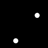
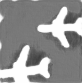
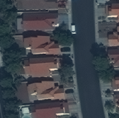
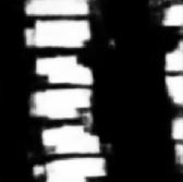
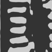
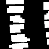
(a)	(b)	(c)	(d)	(e)	(f)	(g)

Figure 6: Extended results for predicted segmentation masks from the Aircraft (row 1), Woolsey (row 2), Well Pad (row 3), and SpaceNet (row 4) datasets using fully-supervised UNet models with ResNet backbones (c-e) and our semi-supervised P2P model (f). All generated masks come from training with Dice loss, besides (e), which is trained with cross entropy loss for comparison. (a) Input image to each model. (b) Pseudo label $\tilde{y}$ used to train P2P. (c) Output from a UNet-101 baseline model. (d) Output from UNet-50. (e) Output from UNet-50 trained with cross-entropy. (f) Output from P2P (ours). (g) Ground Truth labels.

A.2 Localization Guidance ablative study visual results

Input $I_{R}$	Context $I_{ctx}$	Pseudo label $\tilde{y}$	Output $\hat{y}$	Pos. Fake $I_{F_{1}}$	Neg. Fake $I_{F_{2}}$	Ground Truth $y$

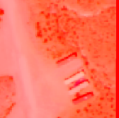
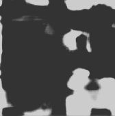
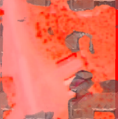
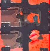
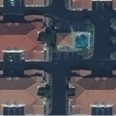
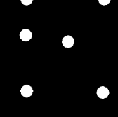
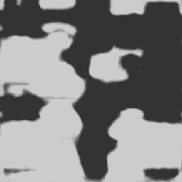
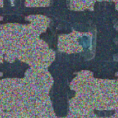
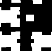
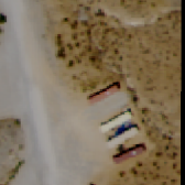
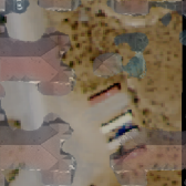
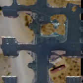
Figure 7: Effect of different transformations on the context image and resulting segmentation mask. Please see Section 5.3 for further details.

In this ablative study we observe the effect that changing the localization guidance buffer size has on the output prediction $\hat{y}$. This buffer size is determined by the centroid size multiplier (csm) variable which is factored into the localization loss for the generator. See Algorithm 1 for more details on the role of csm in the buffer size calculation and localization loss.

Input: constant csm, constant $\Sigma$, constant $\gamma$, constant $\rho$

canvas $\leftarrow$ zeros ;

$p_{geom}\leftarrow\textmd{label}(I_{R})$;

for point $p\in p_{geom}$ do

       $\mu\leftarrow(p_{x},p_{y})$;

       $\textmd{centroid\_raster}\sim MVN(\mu,\Sigma)$;

       $\textmd{canvas}\leftarrow\textmd{element-wise max}(\textmd{canvas},\textmd{centroid\_raster})$;

      

end for

$\textmd{canvas}^{*}\leftarrow\textmd{csm}\cdot\textmd{canvas}$;

$\tilde{y}\leftarrow\textmd{element-wise where}(\textmd{canvas}^{*}\geq\gamma,1,0)$;

$\operatorname{\mathcal{L}}_{loc}\leftarrow\min(\textmd{cross-entropy}(\hat{y},\tilde{y}),\rho)$;

return $\operatorname{\mathcal{L}}_{loc}$

Algorithm 1 Localization loss formulation per image sample $I_{R}$.

In the procedure for deriving $\tilde{y}$, we use a bivariate Gaussian with covariance matrix $\Sigma$ to generate a candidate buffer area around each point label $p$, whose coordinates define the mean. A hyperparameter $\gamma$ is used as a centroid threshold constant to binarize the candidate buffer areas. We employ a threshold parameter $\rho$ to control the influence of the localization loss on the overall generator loss. The csm variable then effectively determines the size of the buffered centroids.

Through experimentation we observe that having a smaller buffer (csm=$7000$) produces a better Dice score and better visual results for most datasets, with the notable exception of the well pads dataset, where having a larger buffer produces a higher Dice score. We argue that this is due to the fact that a larger buffer effectively overpowers the other loss terms in the generator and brings in contextual noise in cases where the buffer extends beyond the object’s bounding geometry, as is the case for planes or smaller buildings but not for well pads which tend to be larger.

A.3 Pre/Post Processing

We use the ArcGIS Pro geospatial software in order to perform input preprocessing on all datasets. Preprocessing consists of modifying image bit depth (we use uint8 for all datasets) as well as cell size adjustments which define the image resolution. We also use ArcGIS Pro to transform the labels (such as for data obtained from the SpaceNet dataset) from .geojson into ESRI .shp files using the JSON to Features geoprocessing (GP) tool. Preprocessing further consists of tiling input rasters into smaller, manageable chips using the Export Training Data for Deep Learning GP tool. Note the preprocessing steps are not needed when directly using our provided datasets.

To produce the actual polygonal outputs (i.e. the Polygons in Points2Polygons), we first apply a threshold of $0.5$ to convert the output $\hat{y}$ to a binary representation before converting the mask to a polygon geometry using the Feature to Polygon GP tool. For certain use cases such as building footprints and well pads we also use the Building Footprint Regularization GP tool to enhance our results.

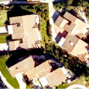
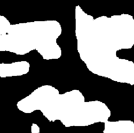
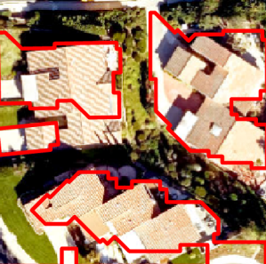
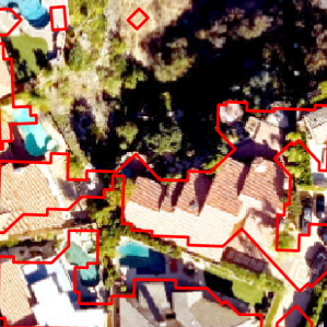
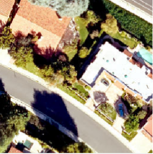
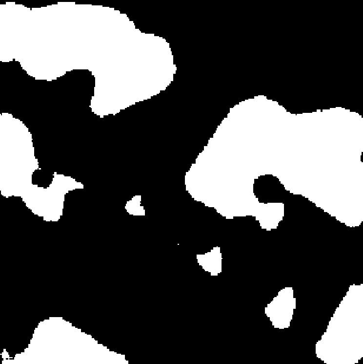
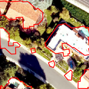
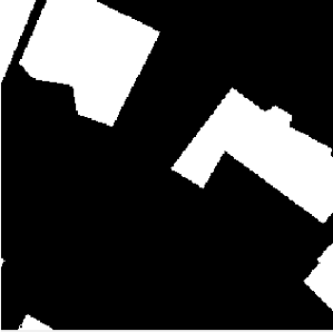
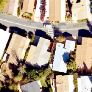
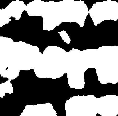
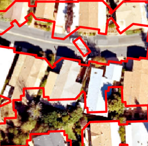
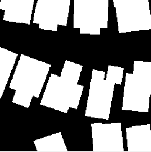
$I_{R}$	$\hat{y}_{bin}$	Regularized Footprint	$y$

Figure 8: Binarized output from the model $\hat{y}_{bin}$ and the output after being post-processed using the Building Footprint Regularization function. Please see Section A.3 for more details.

	$6000$	$7000$	$8000$	$9000$	$10000$
$\tilde{y}$
$\hat{y}$
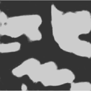
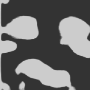
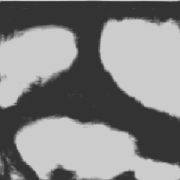
$I_{F_{1}}$
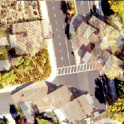
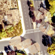
$I_{F_{2}}$

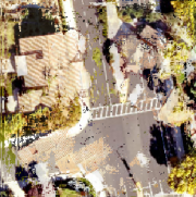
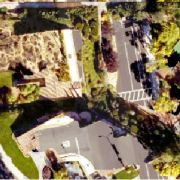
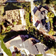
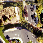
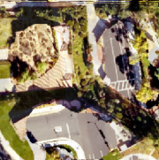
Figure 9: Visual results from the localization guidance ablative study for the Woolsey dataset, for different values of csm.

	$6000$	$7000$	$8000$	$9000$	$10000$
$\tilde{y}$
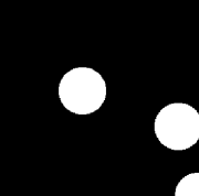
$\hat{y}$
$I_{F_{1}}$
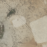
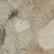
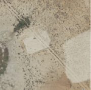
$I_{F_{2}}$

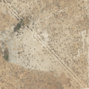
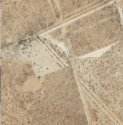
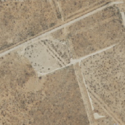
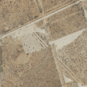
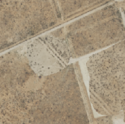
Figure 10: Visual results from the localization guidance ablative study for the Well Pads dataset, for different values of csm.

	$6000$	$7000$	$8000$	$9000$	$10000$
$\tilde{y}$
$\hat{y}$
$I_{F_{1}}$
$I_{F_{2}}$

Figure 11: Visual results from the localization guidance ablative study for the Aircraft dataset, for different values of csm.

	Input $I_{R}$	Pseudo label $\tilde{y}$	Output $\hat{y}$	Pos. Fake $I_{F_{1}}$	Neg. Fake $I_{F_{2}}$	Ground Truth $y$
Airplanes
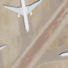
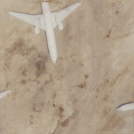
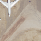
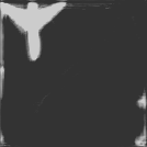
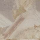
Well Pad
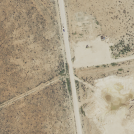
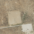
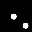
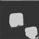
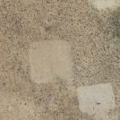
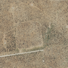
Woolsey
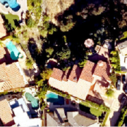
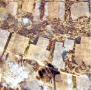
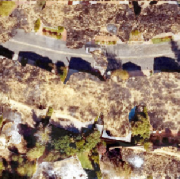
SpaceNet

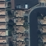
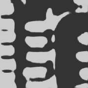
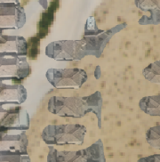
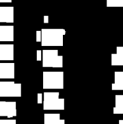
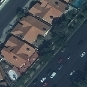
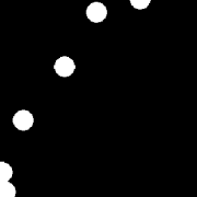
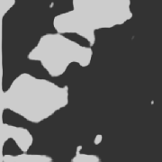
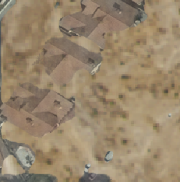
Figure 12: Example segmentation masks and training data for two samples in each dataset.

References

- Ahn and Kwak [2018] J. Ahn and S. Kwak. Learning pixel-level semantic affinity with image-level supervision for weakly supervised semantic segmentation. CoRR, abs/1803.10464, 2018. URL http://arxiv.org/abs/1803.10464.
- Ahn et al. [2019] J. Ahn, S. Cho, and S. Kwak. Weakly supervised learning of instance segmentation with inter-pixel relations. CoRR, abs/1904.05044, 2019. URL http://arxiv.org/abs/1904.05044.
- Bittner et al. [2016] K. Bittner, S. Cui, and P. Reinartz. Building footprint extraction from digital surface models using neural networks. page 100040J, 10 2016. doi: 10.1117/12.2240727.
- Caron et al. [2021] M. Caron, H. Touvron, I. Misra, H. Jégou, J. Mairal, P. Bojanowski, and A. Joulin. Emerging properties in self-supervised vision transformers, 2021.
- Cha et al. [2017] Y.-J. Cha, W. Choi, and O. Buyukozturk. Deep learning-based crack damage detection using convolutional neural networks. Computer-Aided Civil and Infrastructure Engineering, 32:361–378, 03 2017. doi: 10.1111/mice.12263.
- Chawda et al. [2018] C. Chawda, J. Aghav, and S. Udar. Extracting building footprints from satellite images using convolutional neural networks. pages 572–577, 09 2018. doi: 10.1109/ICACCI.2018.8554893.
- Chen et al. [2019] M. Chen, T. Artières, and L. Denoyer. Unsupervised object segmentation by redrawing. In H. Wallach, H. Larochelle, A. Beygelzimer, F. d'Alché-Buc, E. Fox, and R. Garnett, editors, Advances in Neural Information Processing Systems, volume 32. Curran Associates, Inc., 2019. URL https://proceedings.neurips.cc/paper/2019/file/32bbf7b2bc4ed14eb1e9c2580056a989-Paper.pdf.
- Csillik [2017] O. Csillik. Fast segmentation and classification of very high resolution remote sensing data using slic superpixels. Remote Sensing, 9:243, 03 2017. doi: 10.3390/rs9030243.
- Dai et al. [2015] J. Dai, K. He, and J. Sun. Boxsup: Exploiting bounding boxes to supervise convolutional networks for semantic segmentation. CoRR, abs/1503.01640, 2015. URL http://arxiv.org/abs/1503.01640.
- Dhere and Sivaswamy [2021] A. Dhere and J. Sivaswamy. Self-supervised learning for segmentation. CoRR, abs/2101.05456, 2021. URL https://arxiv.org/abs/2101.05456.
- Etten et al. [2018] A. V. Etten, D. Lindenbaum, and T. M. Bacastow. Spacenet: A remote sensing dataset and challenge series. CoRR, abs/1807.01232, 2018. URL http://arxiv.org/abs/1807.01232.
- Fiedler and Alpers [2020] M. Fiedler and A. Alpers. Power-slic: Diagram-based superpixel generation. CoRR, abs/2012.11772, 2020. URL https://arxiv.org/abs/2012.11772.
- Gulgec et al. [2017] N. Gulgec, M. Takáč, and S. Pakzad. Structural Damage Detection Using Convolutional Neural Networks, pages 331–337. 06 2017. ISBN 978-3-319-54857-9. doi: 10.1007/978-3-319-54858-6_33.
- Hartley et al. [2019] T. Hartley, K. A. Sidorov, C. Willis, and A. D. Marshall. Gradient weighted superpixels for interpretability in cnns. CoRR, abs/1908.08997, 2019. URL http://arxiv.org/abs/1908.08997.
- Jaiswal et al. [2020] A. Jaiswal, A. R. Babu, M. Z. Zadeh, D. Banerjee, and F. Makedon. A survey on contrastive self-supervised learning. CoRR, abs/2011.00362, 2020. URL https://arxiv.org/abs/2011.00362.
- Laradji et al. [2019] I. H. Laradji, N. Rostamzadeh, P. O. Pinheiro, D. Vázquez, and M. Schmidt. Instance segmentation with point supervision. CoRR, abs/1906.06392, 2019. URL http://arxiv.org/abs/1906.06392.
- Leyva-Vallina et al. [2021] M. Leyva-Vallina, N. Strisciuglio, and N. Petkov. Generalized contrastive optimization of siamese networks for place recognition. CoRR, abs/2103.06638, 2021. URL https://arxiv.org/abs/2103.06638.
- Li et al. [2018] L. Li, K. G. Jamieson, A. Rostamizadeh, E. Gonina, M. Hardt, B. Recht, and A. Talwalkar. Massively parallel hyperparameter tuning. CoRR, abs/1810.05934, 2018. URL http://arxiv.org/abs/1810.05934.
- Li et al. [2017] W. Li, H. Fu, L. Yu, and A. Cracknell. Deep learning based oil palm tree detection and counting for high-resolution remote sensing images. Remote Sensing, 9(1), 2017. ISSN 2072-4292. doi: 10.3390/rs9010022. URL https://www.mdpi.com/2072-4292/9/1/22.
- Luc et al. [2016] P. Luc, C. Couprie, S. Chintala, and J. Verbeek. Semantic segmentation using adversarial networks. CoRR, abs/1611.08408, 2016. URL http://arxiv.org/abs/1611.08408.
- Neupane et al. [2019] B. Neupane, T. Horanont, and N. Hung. Deep learning based banana plant detection and counting using high-resolution red-green-blue (rgb) images collected from unmanned aerial vehicle (uav). PLOS ONE, 14:e0223906, 10 2019. doi: 10.1371/journal.pone.0223906.
- Oquab et al. [2015] M. Oquab, L. Bottou, I. Laptev, and J. Sivic. Is object localization for free? - weakly-supervised learning with convolutional neural networks. In 2015 IEEE Conference on Computer Vision and Pattern Recognition (CVPR), pages 685–694, 2015. doi: 10.1109/CVPR.2015.7298668.
- Osco et al. [2020] L. Osco, M. dos Santos de Arruda, J. Junior, N. Silva, A. P. Ramos, E. Moriya, N. Imai, D. Pereira, J. Creste, E. Matsubara, J. Li, and W. Gonçalves. A convolutional neural network approach for counting and geolocating citrus-trees in uav multispectral imagery. ISPRS Journal of Photogrammetry and Remote Sensing, 160:97–106, 02 2020. doi: 10.1016/j.isprsjprs.2019.12.010.
- Paul et al. [2020] S. Paul, Y. Tsai, S. Schulter, A. K. Roy-Chowdhury, and M. Chandraker. Domain adaptive semantic segmentation using weak labels. CoRR, abs/2007.15176, 2020. URL https://arxiv.org/abs/2007.15176.
- Porter and Duff [1984] T. Porter and T. Duff. Compositing digital images. SIGGRAPH Comput. Graph., 18(3):253–259, Jan. 1984. ISSN 0097-8930. doi: 10.1145/964965.808606. URL https://doi.org/10.1145/964965.808606.
- Ren et al. [2015] C. Y. Ren, V. A. Prisacariu, and I. D. Reid. gslicr: SLIC superpixels at over 250hz. CoRR, abs/1509.04232, 2015. URL http://arxiv.org/abs/1509.04232.
- Souly et al. [2017] N. Souly, C. Spampinato, and M. Shah. Semi supervised semantic segmentation using generative adversarial network. In 2017 IEEE International Conference on Computer Vision (ICCV), pages 5689–5697, 2017. doi: 10.1109/ICCV.2017.606.
- Wang et al. [2020] S. Wang, W. Chen, S. M. Xie, G. Azzari, and D. B. Lobell. Weakly supervised deep learning for segmentation of remote sensing imagery. Remote Sensing, 12(2), 2020. ISSN 2072-4292. doi: 10.3390/rs12020207. URL https://www.mdpi.com/2072-4292/12/2/207.
- Xia et al. [2017] G. Xia, X. Bai, J. Ding, Z. Zhu, S. J. Belongie, J. Luo, M. Datcu, M. Pelillo, and L. Zhang. DOTA: A large-scale dataset for object detection in aerial images. CoRR, abs/1711.10398, 2017. URL http://arxiv.org/abs/1711.10398.
- Yao et al. [2021] L. Yao, T. Liu, J. Qin, N. Lu, and C. Zhou. Tree counting with high spatial-resolution satellite imagery based on deep neural networks. Ecological Indicators, 125:1–12, 03 2021. doi: 10.1016/j.ecolind.2021.107591.
- Zhu et al. [2019a] H. Zhu, J. Shi, and J. Wu. Pick-and-learn: Automatic quality evaluation for noisy-labeled image segmentation. CoRR, abs/1907.11835, 2019a. URL http://arxiv.org/abs/1907.11835.
- Zhu et al. [2019b] Q. Zhu, C. Liao, H. Hu, X. Mei, and H. Li. Map-net: Multi attending path neural network for building footprint extraction from remote sensed imagery. CoRR, abs/1910.12060, 2019b. URL http://arxiv.org/abs/1910.12060.