Principal Bit Analysis:
Autoencoding with Schur-Concave Loss

Sourbh Bhadane
Cornell University
snb62@cornell.edu
This research was supported by the US National Science Foundation under grants CCF-2008266, CCF-1934985, CCF-1617673, CCF-1846300, CCF-1815893 and the US Army Research Office under grant W911NF-18-1-0426.
   Aaron B. Wagner11footnotemark: 1
Cornell University
wagner@cornell.edu
   Jayadev Acharya11footnotemark: 1
Cornell University
acharya@cornell.edu
Abstract

We consider a linear autoencoder in which the latent variables are quantized, or corrupted by noise, and the constraint is Schur-concave in the set of latent variances. Although finding the optimal encoder/decoder pair for this setup is a nonconvex optimization problem, we show that decomposing the source into its principal components is optimal. If the constraint is strictly Schur-concave and the empirical covariance matrix has only simple eigenvalues, then any optimal encoder/decoder must decompose the source in this way. As one application, we consider a strictly Schur-concave constraint that estimates the number of bits needed to represent the latent variables under fixed-rate encoding, a setup that we call Principal Bit Analysis (PBA). This yields a practical, general-purpose, fixed-rate compressor that outperforms existing algorithms. As a second application, we show that a prototypical autoencoder-based variable-rate compressor is guaranteed to decompose the source into its principal components.

1 Introduction

Autoencoders are an effective method for representation learning and dimensionality reduction. Given a centered dataset 𝒙1,𝒙2,,𝒙ndsubscript𝒙1subscript𝒙2subscript𝒙𝑛superscript𝑑\bm{x}_{1},\bm{x}_{2},\ldots,\bm{x}_{n}\in\mathbb{R}^{d} (i.e., i𝒙i=0subscript𝑖subscript𝒙𝑖0\sum_{i}\bm{x}_{i}=0), an autoencoder (with latent dimension kd𝑘𝑑k\leq d) consists of an encoder f:dk:𝑓maps-tosuperscript𝑑superscript𝑘f:\mathbb{R}^{d}\mapsto\mathbb{R}^{k} and a decoder g:kd:𝑔maps-tosuperscript𝑘superscript𝑑g:\mathbb{R}^{k}\mapsto\mathbb{R}^{d}. The goal is to select f𝑓f and g𝑔g from prespecified classes 𝒞fsubscript𝒞𝑓\mathcal{C}_{f} and 𝒞gsubscript𝒞𝑔\mathcal{C}_{g} respectively such that if a random point 𝒙𝒙\bm{x} is picked from the data set then g(f(𝒙))𝑔𝑓𝒙g(f(\bm{x})) is close to 𝒙𝒙\bm{x} in some sense, for example in mean squared error. If 𝒞fsubscript𝒞𝑓\mathcal{C}_{f} and 𝒞gsubscript𝒞𝑔\mathcal{C}_{g} consist of linear mappings then the autoencoder is called a linear autoencoder.

Autoencoders have achieved striking successes when f𝑓f and g𝑔g are selected through training from the class of functions realized by multilayer perceptrons of a given architecture [HS06]. Yet, the canonical autoencoder formulation described above has a notable failing, namely that for linear autoencoders, optimal choices of f𝑓f and g𝑔g do not necessarily identify the principal components of the dataset; they merely identify the principal subspace [BK88, BH89]. That is, the components of f(𝒙)𝑓𝒙f(\bm{x}) are not necessarily proportional to projections of 𝒙𝒙\bm{x} against the eigenvectors of the covariance matrix

𝑲=def1ni=1n𝒙i𝒙i,superscriptdef𝑲1𝑛superscriptsubscript𝑖1𝑛subscript𝒙𝑖superscriptsubscript𝒙𝑖top\bm{K}\stackrel{{\scriptstyle\mathrm{def}}}{{=}}\frac{1}{n}\sum_{i=1}^{n}\bm{x}_{i}\cdot\bm{x}_{i}^{\top}, (1)

which we assume without loss of generality is full rank. Thus, linear autoencoders do not recover Principal Component Analysis (PCA). The reason for this is that both the objective (the distortion) and the constraint (the dimensionality of the latents) are invariant to an invertible transformation applied after the encoder with its inverse applied before the decoder. It is desirable for linear autoencoders to recover PCA for two reasons. First, from a representation learning standpoint, it guarantees that the autoencoder recovers uncorrelated features. Second, since a conventional linear autoencoder has a large number of globally optimal solutions corresponding to different bases of the principal subspace, it is preferable to eliminate this indeterminism.

Autoencoders are sometimes described as “compressing” the data [San12, BK88, LZW+21, Bis06], even though f𝑓f can be invertible even when k<d𝑘𝑑k<d. We show that by embracing this compression-view, one can obtain autoencoders that are able to recover PCA. Specifically, we consider linear autoencoders with quantized (or, equivalently, noisy) latent variables with a constraint on the estimated number of bits required to transmit the quantized latents under fixed-rate coding. We call this problem Principal Bit Analysis (PBA). The constraint turns out to be a strictly Schur-concave function of the set of variances of the latent variables (see the supplementary for a review of Schur-concavity). Although finding the optimal f𝑓f and g𝑔g for this loss function is a nonconvex optimization problem, we show that for any strictly Schur-concave loss function, an optimal f𝑓f must send projections of the data along the principal components, assuming that the empirical covariance matrix of the data has only simple eigenvalues. That is, imposing a strictly Schur-concave loss in place of a simple dimensionality constraint suffices to ensure recovery of PCA. The idea is that the strict concavity of the loss function eliminates the rotational invariance described above. As we show, even a slight amount of “curvature” in the constraint forces the autoencoder to spread the variances of the latents out as much as possible, resulting in recovery of PCA. If the loss function is merely Schur-concave, then projecting along the principal components is optimal, but not necessarily uniquely so.

Using this theorem, we can efficiently solve PBA. We validate the solution experimentally by using it to construct a fixed-rate compression algorithm for arbitrary vector-valued data sources. We find that the PBA-derived compressor beats existing linear, fixed-rate compressors both in terms of mean squared error, for which it is optimized, and in terms of the structural similarity index measure (SSIM) and downstream classification accuracy, for which it is not.

A number of variable-rate multimedia compressors have recently been proposed that are either related to, or directly inspired by, autoencoders [TAL18, TVJ+17, BLS16, TOH+16, TSCH17, RB17, HRTC19, AMT+17, BMS+18, ZCG+18, ATM+19, BCM+20]. As a second application of our result, we show that for Gaussian sources, a linear form of such a compressor is guaranteed to recover PCA. Thus we show that ideas from compression can be fruitfully fed back into the original autoencoder problem.

The contributions of the paper are

  • We propose a novel linear autoencoder formulation in which the constraint is Schur-concave. We show that this generalizes conventional linear autoencoding.

  • If the constraint is strictly Schur-concave and the covariance matrix of the data has only simple eigenvalues, then we show that the autoencoder provably recovers PCA, providing a new remedy for a known limitation of linear autoencoders.

  • We use the new linear autoencoder formulation to efficiently solve a fixed-rate compression problem that we call Principal Bit Analysis (PBA).

  • We demonstate experimentally that PBA outperforms existing fixed-rate compressors on a variety of data sets and metrics.

  • We show that a linear, variable-rate compressor that is representative of many autoencoder-based compressors in the literature effectively has a strictly Schur-concave loss, and therefore it recovers PCA.

Related Work. Several recent works have examined how linear autoencoders can be modified to guarantee recovery of PCA. Most solutions involve eliminating the invariant global optimal solutions by introducing regularization of some kind. [OSWS20] propose a loss function which adds k𝑘k penalties to recover the k𝑘k principal directions, each corresponding to recovering up to the first ik𝑖𝑘i\leq k principal directions. [KBGS19] show that 2subscript2\ell_{2} regularization helps reduce the symmetry group to the orthogonal group. [BLSG20] further break the symmetry by considering non-uniform 2subscript2\ell_{2} regularization and deterministic dropout. [LNP19] consider a nonlinear autoencoder with a covariance loss term to encourage finding orthogonal directions. Recovering PCA is an important problem even in the stochastic counterpart of autoencoders. [LTGN19] analyze linear variational autoencoders (VAEs) and show that the global optimum of its objective is identical to the global optimum of log marginal likelihood of probabilistic PCA (pPCA). [RZM19] analyze an approximation to the VAE loss function and show that the linear approximation to the decoder is orthogonal.

Our result on variable-rate compressors is connected to the sizable recent literature on compression using autoencoder-like architectures. Representative contributions to the literature were noted above. Those works focus mostly on the empirical performance of deep, nonlinear networks, with a particular emphasis on finding a differentiable proxy for quantization so as to train with stochastic gradient descent. In contrast, this work considers provable properties of the compressors when trained perfectly.

Notation. We denote matrices by bold capital letters e.g. 𝑴𝑴\bm{M}, and vectors by bold small, e.g. 𝒗𝒗\bm{v}. The jthsuperscript𝑗thj^{\text{th}} column of a matrix 𝑴𝑴\bm{M} is denoted by 𝒎jsubscript𝒎𝑗\bm{m}_{j} and the jthsuperscript𝑗thj^{\text{th}} entry of a vector 𝒗𝒗\bm{v} by [𝒗]jsubscriptdelimited-[]𝒗𝑗\left[\bm{v}\right]_{j}. We denote the set {1,2,d}12𝑑\left\{1,2,\cdots d\right\} by [d]delimited-[]𝑑\left[d\right]. A sequence a1,a2,ansubscript𝑎1subscript𝑎2subscript𝑎𝑛a_{1},a_{2},\cdots a_{n} is denoted by {ai}i=1nsuperscriptsubscriptsubscript𝑎𝑖𝑖1𝑛\{a_{i}\}_{i=1}^{n}. We denote the zero column by 𝟎0\bm{0}. Logarithms without specified bases denote natural logarithms.

Organization. The balance of the paper is organized as follows. We describe our constrained linear autoencoder framework in Section 2. This results in an optimization problem that we solve for any Schur-concave constraint in Section 2.1. In Section 3, we recover linear autoencoders and PBA under our framework. We apply the PBA solution to a problem in variable-rate compression of Gaussian sources in Section 4. Section 5 contains experiments comparing the performance of the PBA-based fixed-rate compressor against existing fixed-rate linear compressors on image and audio datasets.

2 Linear Autoencoding with a Schur-Concave Constraint

Throughout this paper we consider 𝒞fsubscript𝒞𝑓\mathcal{C}_{f} and 𝒞gsubscript𝒞𝑔\mathcal{C}_{g} to be the class of linear functions. The functions f𝒞f𝑓subscript𝒞𝑓f\in\mathcal{C}_{f} and g𝒞g𝑔subscript𝒞𝑔g\in\mathcal{C}_{g} can then be represented by d𝑑d-by-d𝑑d matrices, respectively, which we denote by 𝑾𝑾\bm{W} and 𝑻𝑻\bm{T}, respectively. Thus we have

f(𝒙)𝑓𝒙\displaystyle f(\bm{x}) =𝑾𝒙absentsuperscript𝑾top𝒙\displaystyle=\bm{W}^{\top}\bm{x} (2)
g(𝒙)𝑔𝒙\displaystyle g(\bm{x}) =𝑻𝒙.absent𝑻𝒙\displaystyle=\bm{T}\bm{x}. (3)

We wish to design 𝑾𝑾\bm{W} and 𝑻𝑻\bm{T} to minimize the mean squared error when the latent variables 𝑾𝒙superscript𝑾top𝒙\bm{W}^{\top}\bm{x} are quantized, subject to a constraint on the number of bits needed to represent the quantized latents. We accomplish this via two modifications of the canonical autoencoder. First, we perturb the d𝑑d latent variables with zero-mean additive noise with covariance matrix σ2𝑰superscript𝜎2𝑰\sigma^{2}\bm{I}, which we denote by 𝜺.𝜺\bm{\varepsilon}. Thus the input to the decoder is

𝑾𝒙+𝜺superscript𝑾top𝒙𝜺\bm{W}^{\top}\bm{x}+\bm{\varepsilon} (4)

and our objective is to minimize the mean squared error

1ni=1n𝔼𝜺[𝒙i𝑻(𝑾𝒙i+𝜺)22].1𝑛superscriptsubscript𝑖1𝑛subscript𝔼𝜺delimited-[]superscriptsubscriptdelimited-∥∥subscript𝒙𝑖𝑻superscript𝑾topsubscript𝒙𝑖𝜺22\frac{1}{n}\sum\limits_{i=1}^{n}\mathbb{E}_{\bm{\varepsilon}}\left[\left\lVert\bm{x}_{i}-\bm{T}\left(\bm{W}^{\top}\bm{x}_{i}+\bm{\varepsilon}\right)\right\rVert_{2}^{2}\right]. (5)

This is equivalent to quantizing the latents, in the following sense [ZF92]. Let Q()𝑄Q(\cdot) be the function that maps any real number to its nearest integer and ε𝜀\varepsilon be a random variable uniformly distributed over [1/2,1/2]1212[-1/2,1/2]. Then for X𝑋X independent of ε𝜀\varepsilon, the quantities Q(X+ε)ε𝑄𝑋𝜀𝜀Q(X+\varepsilon)-\varepsilon and X+ε𝑋𝜀X+\varepsilon have the same joint distribution with X𝑋X. Thus (5) is exactly the mean squared error if the latents are quantized to the nearest integer and σ2=112superscript𝜎2112\sigma^{2}=\frac{1}{12}, assuming that the quantization is dithered. The overall system is depicted in Fig. 1.

Linear Encoder (𝑾𝑾\bm{W}) Quantizer Linear Decoder (𝑻𝑻\bm{T}) 𝑻(𝑾𝒙i+𝜺)𝑻superscript𝑾topsubscript𝒙𝑖𝜺\bm{T}\left(\bm{W}^{\top}\bm{x}_{i}+\bm{\varepsilon}\right) 𝒙isubscript𝒙𝑖\bm{x}_{i} 𝑾𝒙isuperscript𝑾topsubscript𝒙𝑖\bm{W}^{\top}\bm{x}_{i} 𝑾𝒙i+𝜺superscript𝑾topsubscript𝒙𝑖𝜺\bm{W}^{\top}\bm{x}_{i}+\bm{\varepsilon}
Figure 1: Compression Block Diagram

We wish to constrain the number of bits needed to describe the latent variables. We assume that the j𝑗jth quantized latent is clipped to the interval

((2a)2𝒘j𝑲𝒘j+12,(2a)2𝒘j𝑲𝒘j+12],superscript2𝑎2superscriptsubscript𝒘𝑗top𝑲subscript𝒘𝑗12superscript2𝑎2superscriptsubscript𝒘𝑗top𝑲subscript𝒘𝑗12\left(-\frac{\sqrt{(2a)^{2}\bm{w}_{j}^{\top}\bm{K}\bm{w}_{j}+1}}{2},\frac{\sqrt{(2a)^{2}\bm{w}_{j}^{\top}\bm{K}\bm{w}_{j}+1}}{2}\right],

where a>0𝑎0a>0 is a hyperparameter and the covariance matrix 𝑲𝑲\bm{K} is as defined in (1). The idea is that for sufficiently large a𝑎a, the interval

(a𝒘j𝑲𝒘j,a𝒘j𝑲𝒘j]𝑎superscriptsubscript𝒘𝑗top𝑲subscript𝒘𝑗𝑎superscriptsubscript𝒘𝑗top𝑲subscript𝒘𝑗\left(-a\sqrt{\bm{w}_{j}^{\top}\bm{K}\bm{w}_{j}},a\sqrt{\bm{w}_{j}^{\top}\bm{K}\bm{w}_{j}}\right]

contains the latent with high probability, and adding 111 accounts for the expansion due to the dither. The number of bits needed for the j𝑗jth latent is then

log(4a2𝒘j𝑲𝒘j+1)=12log(4a2𝒘j𝑲𝒘j+1).4superscript𝑎2superscriptsubscript𝒘𝑗top𝑲subscript𝒘𝑗1124superscript𝑎2superscriptsubscript𝒘𝑗top𝑲subscript𝒘𝑗1\displaystyle\log\left(\sqrt{4a^{2}\bm{w}_{j}^{\top}\bm{K}\bm{w}_{j}+1}\right)=\frac{1}{2}\log\left(4a^{2}\bm{w}_{j}^{\top}\bm{K}\bm{w}_{j}+1\right). (6)

We arrive at our optimization problem:

inf𝑾,𝑻subscriptinfimum𝑾𝑻\displaystyle\inf\limits_{\bm{W},\bm{T}} 1ni=1n𝔼𝜺[𝒙i𝑻(𝑾𝒙i+𝜺)22]1𝑛superscriptsubscript𝑖1𝑛subscript𝔼𝜺delimited-[]superscriptsubscriptdelimited-∥∥subscript𝒙𝑖𝑻superscript𝑾topsubscript𝒙𝑖𝜺22\displaystyle\frac{1}{n}\sum\limits_{i=1}^{n}\mathbb{E}_{\bm{\varepsilon}}\left[\left\lVert\bm{x}_{i}-\bm{T}\left(\bm{W}^{\top}\bm{x}_{i}+\bm{\varepsilon}\right)\right\rVert_{2}^{2}\right] (7)
subject to Rj=1d12log(4a2𝒘i𝑲𝒘i+1).𝑅superscriptsubscript𝑗1𝑑124superscript𝑎2superscriptsubscript𝒘𝑖top𝑲subscript𝒘𝑖1\displaystyle R\geq\sum_{j=1}^{d}\frac{1}{2}\log\left(4a^{2}\bm{w}_{i}^{\top}\bm{K}\bm{w}_{i}+1\right).

Note that the function

{𝒘j𝑲𝒘j}j=1dj=1d12log(4a2𝒘i𝑲𝒘i+1)maps-tosuperscriptsubscriptsuperscriptsubscript𝒘𝑗top𝑲subscript𝒘𝑗𝑗1𝑑superscriptsubscript𝑗1𝑑124superscript𝑎2superscriptsubscript𝒘𝑖top𝑲subscript𝒘𝑖1\{\bm{w}_{j}^{\top}\bm{K}\bm{w}_{j}\}_{j=1}^{d}\mapsto\sum_{j=1}^{d}\frac{1}{2}\log\left(4a^{2}\bm{w}_{i}^{\top}\bm{K}\bm{w}_{i}+1\right)

is strictly Schur-concave (see Appendix A for a brief review of Schur-concavity). Our first result only requires that the constraint is Schur-concave in the set of latent variances, so we will consider the more general problem

inf𝑾,𝑻subscriptinfimum𝑾𝑻\displaystyle\inf\limits_{\bm{W},\bm{T}} 1ni=1n𝔼𝜺[𝒙i𝑻(𝑾𝒙i+𝜺)22]1𝑛superscriptsubscript𝑖1𝑛subscript𝔼𝜺delimited-[]superscriptsubscriptdelimited-∥∥subscript𝒙𝑖𝑻superscript𝑾topsubscript𝒙𝑖𝜺22\displaystyle\frac{1}{n}\sum\limits_{i=1}^{n}\mathbb{E}_{\bm{\varepsilon}}\left[\left\lVert\bm{x}_{i}-\bm{T}\left(\bm{W}^{\top}\bm{x}_{i}+\bm{\varepsilon}\right)\right\rVert_{2}^{2}\right] (8)
subject to Rρ({𝒘j𝑲𝒘j}j=1d)𝑅𝜌superscriptsubscriptsuperscriptsubscript𝒘𝑗top𝑲subscript𝒘𝑗𝑗1𝑑\displaystyle R\geq\rho\left(\left\{\bm{w}_{j}^{\top}\bm{K}\bm{w}_{j}\right\}_{j=1}^{d}\right)

where ρ()𝜌\rho(\cdot) is any Schur-concave function.

Expressing the objective in (8) in terms of 𝑲𝑲\bm{K}, the optimization problem reduces to

inf𝑾,𝑻subscriptinfimum𝑾𝑻\displaystyle\inf\limits_{\bm{W},\bm{T}} tr(𝑲)2tr(𝑲𝑾𝑻)+tr(𝑻(𝑾𝑲𝑾+σ2𝑰)𝑻)tr𝑲2tr𝑲𝑾superscript𝑻toptr𝑻superscript𝑾top𝑲𝑾superscript𝜎2𝑰superscript𝑻top\displaystyle\text{tr}\left(\bm{K}\right)-2\text{tr}\left(\bm{K}\bm{W}\bm{T}^{\top}\right)+\text{tr}\left(\bm{T}\left(\bm{W}^{\top}\bm{K}\bm{W}+\sigma^{2}\bm{I}\right)\bm{T}^{\top}\right) (9)
subject to Rρ({𝒘j𝑲𝒘j}j=1d).𝑅𝜌superscriptsubscriptsuperscriptsubscript𝒘𝑗top𝑲subscript𝒘𝑗𝑗1𝑑\displaystyle R\geq\rho\left(\left\{\bm{w}_{j}^{\top}\bm{K}\bm{w}_{j}\right\}_{j=1}^{d}\right).

Since 𝑻𝑻\bm{T} does not appear in the rate constraint, the optimal 𝑻𝑻\bm{T} can be viewed as the Linear Least Squares Estimate (LLSE) of a random 𝒙𝒙\bm{x} given 𝑾𝒙+𝜺superscript𝑾top𝒙𝜺\bm{W}^{\top}\bm{x}+\bm{\varepsilon}. Therefore, the optimal decoder, 𝑻superscript𝑻\bm{T}^{*} for a given encoder 𝑾𝑾\bm{W} is (e.g. [Kay98]):

𝑻=𝑲𝑾(𝑾𝑲𝑾+σ2𝑰)1.superscript𝑻𝑲𝑾superscriptsuperscript𝑾top𝑲𝑾superscript𝜎2𝑰1\bm{T}^{*}=\bm{K}\bm{W}(\bm{W}^{\top}\bm{K}\bm{W}+\sigma^{2}\bm{I})^{-1}. (10)

Substituting for 𝑻𝑻\bm{T} in (9) yields an optimization problem over only 𝑾𝑾\bm{W}

inf𝑾subscriptinfimum𝑾\displaystyle\inf\limits_{\bm{W}} tr(𝑲)tr(𝑲𝑾(𝑾𝑲𝑾+σ2𝑰)1𝑾𝑲)tr𝑲tr𝑲𝑾superscriptsuperscript𝑾top𝑲𝑾superscript𝜎2𝑰1superscript𝑾top𝑲\displaystyle\text{tr}(\bm{K})-\text{tr}(\bm{K}\bm{W}(\bm{W}^{\top}\bm{K}\bm{W}+\sigma^{2}\bm{I})^{-1}\bm{W}^{\top}\bm{K}) (11)
subject to Rρ({𝒘j𝑲𝒘j}j=1d).𝑅𝜌superscriptsubscriptsuperscriptsubscript𝒘𝑗top𝑲subscript𝒘𝑗𝑗1𝑑\displaystyle R\geq\rho\left(\left\{\bm{w}_{j}^{\top}\bm{K}\bm{w}_{j}\right\}_{j=1}^{d}\right).

This problem is nonconvex in general. In the following subsection, we prove a structural result about the problem for a Schur-concave ρ𝜌\rho. Namely, we show that the nonzero rows of 𝑾𝑾\bm{W} must be eigenvectors of 𝑲𝑲\bm{K}. In Section 3, we solve the problem for the specific choice of ρ𝜌\rho in (7). We also show how this generalizes conventional linear autoencoders.

2.1 Optimal Autoencoding with a Schur-Concave Constraint

The following is the main theoretical result of the paper.

Theorem 1.

For Schur-concave ρ:0d0:𝜌superscriptsubscriptabsent0𝑑subscriptabsent0\rho:\mathbb{R}_{\geq 0}^{d}\rightarrow\mathbb{R}_{\geq 0} and R>0𝑅0R>0, the set of matrices whose nonzero columns are eigenvectors of the covariance matrix 𝐊𝐊\bm{K} is optimal for (11). If ρ𝜌\rho is strictly Schur-concave and 𝐊𝐊\bm{K} contains distinct eigenvalues, this set contains all optimal solutions of (11).

Proof.

Let the eigenvalues of 𝑲𝑲\bm{K} be {σi2}i=1dsuperscriptsubscriptsuperscriptsubscript𝜎𝑖2𝑖1𝑑\{\sigma_{i}^{2}\}_{i=1}^{d} with σ12σ22σd2superscriptsubscript𝜎12superscriptsubscript𝜎22subscriptsuperscript𝜎2𝑑\sigma_{1}^{2}\geq\sigma_{2}^{2}\geq\ldots\geq\sigma^{2}_{d}. Let the eigendecomposition of 𝑲𝑲\bm{K} be given by 𝑲=𝑼𝚺𝑼𝑲𝑼𝚺superscript𝑼top\bm{K}=\bm{U}\bm{\Sigma}\bm{U}^{\top} where 𝑼𝑼\bm{U} is an orthogonal matrix whose columns are the eigenvectors of 𝑲𝑲\bm{K} and 𝚺𝚺\bm{\Sigma} is a diagonal matrix with entries {σi2}i=1dsuperscriptsubscriptsuperscriptsubscript𝜎𝑖2𝑖1𝑑\left\{\sigma_{i}^{2}\right\}_{i=1}^{d}.

We first prove that the optimal value of (11) can be achieved by a 𝑾𝑾\bm{W} such that 𝑾𝑲𝑾superscript𝑾top𝑲𝑾\bm{W}^{\top}\bm{K}\bm{W} is a diagonal matrix. Let 𝑾~=𝑾𝑸~𝑾𝑾𝑸\widetilde{\bm{W}}=\bm{W}\bm{Q} where 𝑸𝑸\bm{Q} is the orthogonal matrix obtained from the eigendecomposition of 𝑾𝑲𝑾superscript𝑾top𝑲𝑾\bm{W}^{\top}\bm{K}\bm{W} i.e.,

𝑾𝑲𝑾=𝑸𝚲𝑸,superscript𝑾top𝑲𝑾𝑸𝚲superscript𝑸top\bm{W}^{\top}\bm{K}\bm{W}=\bm{Q}\bm{\Lambda}\bm{Q}^{\top},

where 𝚲𝚲\bm{\Lambda} is a diagonal matrix formed from the eigenvalues of 𝑾𝑲𝑾superscript𝑾top𝑲𝑾\bm{W}^{\top}\bm{K}\bm{W}. Note that

tr(𝑲𝑾~(𝑾~𝑲𝑾~+σ2𝑰)1𝑾~𝑲)tr𝑲~𝑾superscriptsuperscript~𝑾top𝑲~𝑾superscript𝜎2𝑰1superscript~𝑾top𝑲\displaystyle\text{tr}\left(\bm{K}\widetilde{\bm{W}}\left(\widetilde{\bm{W}}^{\top}\bm{K}\widetilde{\bm{W}}+\sigma^{2}\bm{I}\right)^{-1}\widetilde{\bm{W}}^{\top}\bm{K}\right) =tr(𝑲𝑾𝑸(𝚲+σ2𝑰)1𝑸𝑾𝑲)absenttr𝑲𝑾𝑸superscript𝚲superscript𝜎2𝑰1superscript𝑸topsuperscript𝑾top𝑲\displaystyle=\text{tr}\left(\bm{K}\bm{W}\bm{Q}\left(\bm{\Lambda}+\sigma^{2}\bm{I}\right)^{-1}\bm{Q}^{\top}\bm{W}^{\top}\bm{K}\right)
=tr(𝑲𝑾(𝑸𝚲𝑸+σ2𝑸𝑸)1𝑾𝑲).absenttr𝑲𝑾superscript𝑸𝚲superscript𝑸topsuperscript𝜎2𝑸superscript𝑸top1superscript𝑾top𝑲\displaystyle=\text{tr}\left(\bm{K}\bm{W}\left(\bm{Q}\bm{\Lambda}\bm{Q}^{\top}+\sigma^{2}\bm{Q}\bm{Q}^{\top}\right)^{-1}\bm{W}^{\top}\bm{K}\right).

Since 𝑸𝚲𝑸=𝑾𝑲𝑾𝑸𝚲superscript𝑸topsuperscript𝑾top𝑲𝑾\bm{Q}\bm{\Lambda}\bm{Q}^{\top}=\bm{W}^{\top}\bm{K}\bm{W} and 𝑸𝑸=𝑰𝑸superscript𝑸top𝑰\bm{Q}\bm{Q}^{\top}=\bm{I}, the objective remains the same. We now show that the constraint is only improved. Denoting the eigenvalues of 𝑾𝑲𝑾superscript𝑾top𝑲𝑾\bm{W}^{\top}\bm{K}\bm{W} by {νj}j=1dsuperscriptsubscriptsubscript𝜈𝑗𝑗1𝑑\left\{\nu_{j}\right\}_{j=1}^{d}, we have

ρ({𝒘~j𝑲𝒘~j}j=1d)=ρ({𝒒j𝑾𝑲𝑾𝒒j}j=1d)=ρ({νj}j=1d).𝜌superscriptsubscriptsuperscriptsubscript~𝒘𝑗top𝑲subscript~𝒘𝑗𝑗1𝑑𝜌superscriptsubscriptsuperscriptsubscript𝒒𝑗topsuperscript𝑾top𝑲𝑾subscript𝒒𝑗𝑗1𝑑𝜌superscriptsubscriptsubscript𝜈𝑗𝑗1𝑑\rho\left(\left\{\widetilde{\bm{w}}_{j}^{\top}\bm{K}\widetilde{\bm{w}}_{j}\right\}_{j=1}^{d}\right)=\rho\left(\left\{\bm{q}_{j}^{\top}\bm{W}^{\top}\bm{K}\bm{W}\bm{q}_{j}\right\}_{j=1}^{d}\right)=\rho\left(\left\{\nu_{j}\right\}_{j=1}^{d}\right).

Now since the eigenvalues of a Hermitian matrix majorize its diagonal elements by the Schur-Horn theorem [HJ13, Theorem 4.3.45],

{𝒘j𝑲𝒘j}j=1d{νj}j=1d.precedessuperscriptsubscriptsuperscriptsubscript𝒘𝑗top𝑲subscript𝒘𝑗𝑗1𝑑superscriptsubscriptsubscript𝜈𝑗𝑗1𝑑\left\{\bm{w}_{j}^{\top}\bm{K}\bm{w}_{j}\right\}_{j=1}^{d}\prec\left\{\nu_{j}\right\}_{j=1}^{d}.

Since ρ𝜌\rho is Schur-concave, this implies

ρ({𝒘j𝑲𝒘j}j=1d)ρ({νj}j=1d)=ρ({𝒘~j𝑲𝒘~i}j=1d).𝜌superscriptsubscriptsuperscriptsubscript𝒘𝑗top𝑲subscript𝒘𝑗𝑗1𝑑𝜌superscriptsubscriptsubscript𝜈𝑗𝑗1𝑑𝜌superscriptsubscriptsuperscriptsubscript~𝒘𝑗top𝑲subscript~𝒘𝑖𝑗1𝑑\rho\left(\left\{\bm{w}_{j}^{\top}\bm{K}\bm{w}_{j}\right\}_{j=1}^{d}\right)\geq\rho\left(\left\{\nu_{j}\right\}_{j=1}^{d}\right)=\rho\left(\left\{\widetilde{\bm{w}}_{j}^{\top}\bm{K}\widetilde{\bm{w}}_{i}\right\}_{j=1}^{d}\right).

Therefore, if ρ𝜌\rho is Schur-concave, the rate constraint can only improve. This implies an optimal solution can be attained when 𝑾𝑾\bm{W} is such that 𝑾𝑲𝑾superscript𝑾top𝑲𝑾\bm{W}^{\top}\bm{K}\bm{W} is diagonal. If ρ𝜌\rho is strictly Schur-concave, the rate constraint strictly improves implying that the optimal 𝑾𝑾\bm{W} must be such that 𝑾𝑲𝑾superscript𝑾top𝑲𝑾\bm{W}^{\top}\bm{K}\bm{W} is diagonal. This implies that

tr(𝑲𝑾(𝑾𝑲𝑾+σ2𝑰)1𝑾𝑲)tr𝑲𝑾superscriptsuperscript𝑾top𝑲𝑾superscript𝜎2𝑰1superscript𝑾top𝑲\displaystyle\text{tr}\left(\bm{K}\bm{W}\left(\bm{W}^{\top}\bm{K}\bm{W}+\sigma^{2}\bm{I}\right)^{-1}\bm{W}^{\top}\bm{K}\right) =tr(𝑾𝑲2𝑾(𝑾𝑲𝑾+σ2𝑰)1)absenttrsuperscript𝑾topsuperscript𝑲2𝑾superscriptsuperscript𝑾top𝑲𝑾superscript𝜎2𝑰1\displaystyle=\text{tr}\left(\bm{W}^{\top}\bm{K}^{2}\bm{W}\left(\bm{W}^{\top}\bm{K}\bm{W}+\sigma^{2}\bm{I}\right)^{-1}\right)
=i=1d𝒘i𝑲2𝒘iσ2+𝒘i𝑲𝒘i.absentsuperscriptsubscript𝑖1𝑑superscriptsubscript𝒘𝑖topsuperscript𝑲2subscript𝒘𝑖superscript𝜎2superscriptsubscript𝒘𝑖top𝑲subscript𝒘𝑖\displaystyle=\sum\limits_{i=1}^{d}\frac{\bm{w}_{i}^{\top}\bm{K}^{2}\bm{w}_{i}}{\sigma^{2}+\bm{w}_{i}^{\top}\bm{K}\bm{w}_{i}}.

Note that minimizing the objective in (11) is equivalent to maximizing the above expression. Perform the change of variable

𝒘jsubscript𝒘𝑗\displaystyle\bm{w}_{j} {(𝑲1/2𝒘j𝑲1/2𝒘j,𝑲1/2𝒘j2)if 𝑲1/2𝒘j𝟎(𝟎,0)if 𝑲1/2𝒘j=𝟎maps-toabsentcasessuperscript𝑲12subscript𝒘𝑗normsuperscript𝑲12subscript𝒘𝑗superscriptnormsuperscript𝑲12subscript𝒘𝑗2if 𝑲1/2𝒘j𝟎00if 𝑲1/2𝒘j=𝟎\displaystyle\mapsto\begin{cases}\left(\frac{\bm{K}^{1/2}\bm{w}_{j}}{||\bm{K}^{1/2}\bm{w}_{j}||},||\bm{K}^{1/2}\bm{w}_{j}||^{2}\right)&\text{if $\bm{K}^{1/2}\bm{w}_{j}\neq\bm{0}$}\\ (\bm{0},0)&\text{if $\bm{K}^{1/2}\bm{w}_{j}=\bm{0}$}\end{cases}
=(𝒚j,yj).absentsubscript𝒚𝑗subscript𝑦𝑗\displaystyle=(\bm{y}_{j},y_{j}).

The assumption that 𝑾𝑲𝑾superscript𝑾top𝑲𝑾\bm{W}^{\top}\bm{K}\bm{W} is diagonal and the normalization in the definition of 𝒚jsubscript𝒚𝑗\bm{y}_{j} implies that

𝒀=[𝒚1𝒚2,,𝒚d]𝒀subscript𝒚1subscript𝒚2subscript𝒚𝑑\bm{Y}=[\bm{y}_{1}\bm{y}_{2},\cdots,\bm{y}_{d}]

is a matrix whose nonzero columns form an orthonormal set. Rewriting the objective in terms of the (𝒚j,yj)subscript𝒚𝑗subscript𝑦𝑗(\bm{y}_{j},y_{j}), we have

i=1d𝒘i𝑲2𝒘iσ2+𝒘i𝑲𝒘i=i=1d𝒚i𝑲𝒚iyiσ2+yi=i=1d𝒚i𝑲𝒚imi,superscriptsubscript𝑖1𝑑superscriptsubscript𝒘𝑖topsuperscript𝑲2subscript𝒘𝑖superscript𝜎2superscriptsubscript𝒘𝑖top𝑲subscript𝒘𝑖superscriptsubscript𝑖1𝑑superscriptsubscript𝒚𝑖top𝑲subscript𝒚𝑖subscript𝑦𝑖superscript𝜎2subscript𝑦𝑖superscriptsubscript𝑖1𝑑superscriptsubscript𝒚𝑖top𝑲subscript𝒚𝑖subscript𝑚𝑖\sum\limits_{i=1}^{d}\frac{\bm{w}_{i}^{\top}\bm{K}^{2}\bm{w}_{i}}{\sigma^{2}+\bm{w}_{i}^{\top}\bm{K}\bm{w}_{i}}=\sum\limits_{i=1}^{d}\bm{y}_{i}^{\top}\bm{K}\bm{y}_{i}\frac{y_{i}}{\sigma^{2}+y_{i}}=\sum\limits_{i=1}^{d}\bm{y}_{i}^{\top}\bm{K}\bm{y}_{i}m_{i}, (12)

where mi=yiσ2+yisubscript𝑚𝑖subscript𝑦𝑖superscript𝜎2subscript𝑦𝑖m_{i}=\frac{y_{i}}{\sigma^{2}+y_{i}}. Observe that under this new parametrization, the constraint only depends on {yi}i=1dsuperscriptsubscriptsubscript𝑦𝑖𝑖1𝑑\{y_{i}\}_{i=1}^{d}. Without loss of generality, we assume that y1y2ydsubscript𝑦1subscript𝑦2subscript𝑦𝑑y_{1}\geq y_{2}\geq\cdots\geq y_{d}, implying that m1m2mdsubscript𝑚1subscript𝑚2subscript𝑚𝑑m_{1}\geq m_{2}\geq\cdots\geq m_{d}. We now prove that for given {yi}i=1dsuperscriptsubscriptsubscript𝑦𝑖𝑖1𝑑\{y_{i}\}_{i=1}^{d}, choosing the 𝒚isubscript𝒚𝑖\bm{y}_{i} along the eigenvectors of 𝑲𝑲\bm{K} is optimal.

Denote the diagonal elements of 𝒀𝑲𝒀superscript𝒀top𝑲𝒀\bm{Y}^{\top}\bm{K}\bm{Y} by {λi2}i=1dsuperscriptsubscriptsuperscriptsubscript𝜆𝑖2𝑖1𝑑\{\lambda_{i}^{2}\}_{i=1}^{d} and let {λi,2}i=1dsuperscriptsubscriptsuperscriptsubscript𝜆𝑖2𝑖1𝑑\{\lambda_{i,\downarrow}^{2}\}_{i=1}^{d} denote the same diagonal elements arranged in descending order. Denote the eigenvalues of 𝒀𝑲𝒀superscript𝒀top𝑲𝒀\bm{Y}^{\top}\bm{K}\bm{Y} by {μi2}i=1dsuperscriptsubscriptsuperscriptsubscript𝜇𝑖2𝑖1𝑑\{\mu_{i}^{2}\}_{i=1}^{d} where μ1μ2μdsubscript𝜇1subscript𝜇2subscript𝜇𝑑\mu_{1}\geq\mu_{2}\geq\cdots\geq\mu_{d}. Again invoking the Schur-Horn theorem, the eigenvalues of 𝒀𝑲𝒀superscript𝒀top𝑲𝒀\bm{Y}^{\top}\bm{K}\bm{Y} majorize its diagonal entries

{λi2}i=1d{μi2}i=1d.precedessuperscriptsubscriptsuperscriptsubscript𝜆𝑖2𝑖1𝑑superscriptsubscriptsuperscriptsubscript𝜇𝑖2𝑖1𝑑\left\{\lambda_{i}^{2}\right\}_{i=1}^{d}\prec\left\{\mu_{i}^{2}\right\}_{i=1}^{d}. (13)

Substituting λi2=𝒚i𝑲𝒚isuperscriptsubscript𝜆𝑖2superscriptsubscript𝒚𝑖top𝑲subscript𝒚𝑖\lambda_{i}^{2}=\bm{y}_{i}^{\top}\bm{K}\bm{y}_{i} in (12), we have

i=1dλi2mi(a)i=1dλi,2misuperscript𝑎superscriptsubscript𝑖1𝑑superscriptsubscript𝜆𝑖2subscript𝑚𝑖superscriptsubscript𝑖1𝑑superscriptsubscript𝜆𝑖2subscript𝑚𝑖\displaystyle\sum\limits_{i=1}^{d}\lambda_{i}^{2}m_{i}\stackrel{{\scriptstyle(a)}}{{\leq}}\sum\limits_{i=1}^{d}\lambda_{i,\downarrow}^{2}m_{i} =λ1,2m1+i=2d(j=1iλj,2j=1i1λj,2)miabsentsuperscriptsubscript𝜆12subscript𝑚1superscriptsubscript𝑖2𝑑superscriptsubscript𝑗1𝑖superscriptsubscript𝜆𝑗2superscriptsubscript𝑗1𝑖1superscriptsubscript𝜆𝑗2subscript𝑚𝑖\displaystyle=\lambda_{1,\downarrow}^{2}m_{1}+\sum\limits_{i=2}^{d}\left(\sum\limits_{j=1}^{i}\lambda_{j,\downarrow}^{2}-\sum\limits_{j=1}^{i-1}\lambda_{j,\downarrow}^{2}\right)m_{i}
=λ1,2m1+i=2dmij=1iλj,2i=2dmij=1i1λj,2absentsuperscriptsubscript𝜆12subscript𝑚1superscriptsubscript𝑖2𝑑subscript𝑚𝑖superscriptsubscript𝑗1𝑖superscriptsubscript𝜆𝑗2superscriptsubscript𝑖2𝑑subscript𝑚𝑖superscriptsubscript𝑗1𝑖1superscriptsubscript𝜆𝑗2\displaystyle=\lambda_{1,\downarrow}^{2}m_{1}+\sum\limits_{i=2}^{d}m_{i}\sum\limits_{j=1}^{i}\lambda_{j,\downarrow}^{2}-\sum\limits_{i=2}^{d}m_{i}\sum\limits_{j=1}^{i-1}\lambda_{j,\downarrow}^{2}
=λ1,2(m1m2)+md(j=1dλj,2)+i=2d1(mimi+1)j=1iλj,2absentsuperscriptsubscript𝜆12subscript𝑚1subscript𝑚2subscript𝑚𝑑superscriptsubscript𝑗1𝑑superscriptsubscript𝜆𝑗2superscriptsubscript𝑖2𝑑1subscript𝑚𝑖subscript𝑚𝑖1superscriptsubscript𝑗1𝑖superscriptsubscript𝜆𝑗2\displaystyle=\lambda_{1,\downarrow}^{2}(m_{1}-m_{2})+m_{d}\left(\sum\limits_{j=1}^{d}\lambda_{j,\downarrow}^{2}\right)+\sum\limits_{i=2}^{d-1}\left(m_{i}-m_{i+1}\right)\sum\limits_{j=1}^{i}\lambda_{j,\downarrow}^{2}
(b)μ12(m1m2)+md(j=1dμj2)+i=2d1(mimi+1)j=1iμj2superscript𝑏absentsuperscriptsubscript𝜇12subscript𝑚1subscript𝑚2subscript𝑚𝑑superscriptsubscript𝑗1𝑑superscriptsubscript𝜇𝑗2superscriptsubscript𝑖2𝑑1subscript𝑚𝑖subscript𝑚𝑖1superscriptsubscript𝑗1𝑖superscriptsubscript𝜇𝑗2\displaystyle\stackrel{{\scriptstyle(b)}}{{\leq}}\mu_{1}^{2}(m_{1}-m_{2})+m_{d}\left(\sum\limits_{j=1}^{d}\mu_{j}^{2}\right)+\sum\limits_{i=2}^{d-1}(m_{i}-m_{i+1})\sum\limits_{j=1}^{i}\mu_{j}^{2}
(c)σ12(m1m2)+md(j=1dσj2)+i=2d1(mimi+1)j=1iσj2superscript𝑐absentsuperscriptsubscript𝜎12subscript𝑚1subscript𝑚2subscript𝑚𝑑superscriptsubscript𝑗1𝑑superscriptsubscript𝜎𝑗2superscriptsubscript𝑖2𝑑1subscript𝑚𝑖subscript𝑚𝑖1superscriptsubscript𝑗1𝑖superscriptsubscript𝜎𝑗2\displaystyle\stackrel{{\scriptstyle(c)}}{{\leq}}\sigma_{1}^{2}(m_{1}-m_{2})+m_{d}\left(\sum\limits_{j=1}^{d}\sigma_{j}^{2}\right)+\sum\limits_{i=2}^{d-1}(m_{i}-m_{i+1})\sum\limits_{j=1}^{i}\sigma_{j}^{2}
=i=1dσi2mi,absentsuperscriptsubscript𝑖1𝑑superscriptsubscript𝜎𝑖2subscript𝑚𝑖\displaystyle=\sum\limits_{i=1}^{d}\sigma_{i}^{2}m_{i},

where inequality (a)𝑎(a) follows from the assumption that m1m2mdsubscript𝑚1subscript𝑚2subscript𝑚𝑑m_{1}\geq m_{2}\geq\cdots\geq m_{d}, and (b)𝑏(b) from the definition in (13). Since 𝒀𝒀\bm{Y}’s nonzero columns form an orthonormal set, the eigenvalues of 𝒀𝑲𝒀superscript𝒀top𝑲𝒀\bm{Y}^{\top}\bm{K}\bm{Y}, when arranged in descending order, are at most the eigenvalues of 𝑲𝑲\bm{K} from Corollary 4.3.37 in [HJ13], and therefore (c)𝑐(c) follows.

This upper bound is attained when 𝒚i=𝒖isubscript𝒚𝑖subscript𝒖𝑖\bm{y}_{i}=\bm{u}_{i} for nonzero yisubscript𝑦𝑖y_{i}, where 𝒖isubscript𝒖𝑖\bm{u}_{i} is the normalized eigenvector of 𝑲𝑲\bm{K} corresponding to eigenvalue σi2superscriptsubscript𝜎𝑖2\sigma_{i}^{2}. To see this, note that when 𝒚i=𝒖isubscript𝒚𝑖subscript𝒖𝑖\bm{y}_{i}=\bm{u}_{i}, λi2=μi2=σi2superscriptsubscript𝜆𝑖2superscriptsubscript𝜇𝑖2superscriptsubscript𝜎𝑖2\lambda_{i}^{2}=\mu_{i}^{2}=\sigma_{i}^{2}. From the definition of 𝒚i,𝒘i=𝑲1/2𝒖iyi=𝒖iyiσisubscript𝒚𝑖subscript𝒘𝑖superscript𝑲12subscript𝒖𝑖subscript𝑦𝑖subscript𝒖𝑖subscript𝑦𝑖subscript𝜎𝑖\bm{y}_{i},\bm{w}_{i}=\bm{K}^{-1/2}\bm{u}_{i}\sqrt{y_{i}}=\bm{u}_{i}\frac{\sqrt{y_{i}}}{\sigma_{i}}. Therefore, for a Schur-concave ρ𝜌\rho, the set of matrices whose nonzero columns are eigenvectors of 𝑲𝑲\bm{K} is optimal. We now prove that for a strictly Schur-concave ρ𝜌\rho, if 𝑲𝑲\bm{K} has distinct eigenvalues, this set contains all of the optimal solutions 𝑾𝑾\bm{W}.

We know that for a fixed y1y2ydsubscript𝑦1subscript𝑦2subscript𝑦𝑑y_{1}\geq y_{2}\geq\cdots\geq y_{d}, (implying a fixed m1m2mdsubscript𝑚1subscript𝑚2subscript𝑚𝑑m_{1}\geq m_{2}\geq\cdots\geq m_{d}) the upper bound i=1dσi2misuperscriptsubscript𝑖1𝑑superscriptsubscript𝜎𝑖2subscript𝑚𝑖\sum\limits_{i=1}^{d}\sigma_{i}^{2}m_{i} is attained by the previous choice of 𝒚isubscript𝒚𝑖\bm{y}_{i}. Note that if all nonzero misubscript𝑚𝑖m_{i} are distinct, equality in (b)𝑏(b) and (c)𝑐(c) is attained if and only if the nonzero diagonal elements of 𝒀𝑲𝒀superscript𝒀top𝑲𝒀\bm{Y}^{\top}\bm{K}\bm{Y} equal the corresponding eigenvalues of 𝑲𝑲\bm{K}. This implies that, if all nonzero misubscript𝑚𝑖m_{i} are distinct, the upper bound is attained if and only if 𝒚i=𝒖isubscript𝒚𝑖subscript𝒖𝑖\bm{y}_{i}=\bm{u}_{i} for nonzero yisubscript𝑦𝑖y_{i}. Therefore, it is sufficient to prove that for the following optimization problem

sup{yi0}subscriptsupremumsubscript𝑦𝑖0\displaystyle\sup\limits_{\{y_{i}\geq 0\}} i=1dσi2yiσ2+yisuperscriptsubscript𝑖1𝑑superscriptsubscript𝜎𝑖2subscript𝑦𝑖superscript𝜎2subscript𝑦𝑖\displaystyle\sum\limits_{i=1}^{d}\sigma_{i}^{2}\frac{y_{i}}{\sigma^{2}+y_{i}} (14)
subject to Rρ({yi}i=1d),𝑅𝜌superscriptsubscriptsubscript𝑦𝑖𝑖1𝑑\displaystyle R\geq\rho\left(\left\{y_{i}\right\}_{i=1}^{d}\right),

any optimal {yi}subscript𝑦𝑖\{y_{i}\} must be such that the nonzero yisubscript𝑦𝑖y_{i} are distinct. Firstly, note that since σ12>σ22>>σd2superscriptsubscript𝜎12superscriptsubscript𝜎22superscriptsubscript𝜎𝑑2\sigma_{1}^{2}>\sigma_{2}^{2}>\cdots>\sigma_{d}^{2}, we must have y1y2ydsubscript𝑦1subscript𝑦2subscript𝑦𝑑y_{1}\geq y_{2}\geq\cdots\geq y_{d}. Assume to the contrary that for an optimal {yi}i=1dsuperscriptsubscriptsubscript𝑦𝑖𝑖1𝑑\{y_{i}\}_{i=1}^{d} there exists 1j,<dformulae-sequence1𝑗𝑑1\leq j,\ell<d such that yj1>yj=yj+1=yj+2==yj+>yj++10subscript𝑦𝑗1subscript𝑦𝑗subscript𝑦𝑗1subscript𝑦𝑗2subscript𝑦𝑗subscript𝑦𝑗10y_{j-1}>y_{j}=y_{j+1}=y_{j+2}=\cdots=y_{j+\ell}>y_{j+\ell+1}\geq 0, where y0subscript𝑦0y_{0} is chosen to be any real number strictly greater than y1subscript𝑦1y_{1} and yd+1=0subscript𝑦𝑑10y_{d+1}=0. Take δ>0𝛿0\delta>0 small. Denote a new sequence {yi}i=1dsuperscriptsubscriptsubscriptsuperscript𝑦𝑖𝑖1𝑑\{y^{\prime}_{i}\}_{i=1}^{d} where yj=yj+δ,yj+=yj+δformulae-sequencesubscriptsuperscript𝑦𝑗subscript𝑦𝑗𝛿subscriptsuperscript𝑦𝑗subscript𝑦𝑗𝛿y^{\prime}_{j}=y_{j}+\delta,y^{\prime}_{j+\ell}=y_{j+\ell}-\delta and yi=yisubscriptsuperscript𝑦𝑖subscript𝑦𝑖y^{\prime}_{i}=y_{i} for 1id1𝑖𝑑1\leq i\leq d with ij𝑖𝑗i\neq j and j+𝑗j+\ell. Since ρ𝜌\rho is strictly Schur-concave, the constraint is strictly improved,

ρ({yi}i=1d)<ρ({yi}i=1d).𝜌superscriptsubscriptsubscriptsuperscript𝑦𝑖𝑖1𝑑𝜌superscriptsubscriptsubscript𝑦𝑖𝑖1𝑑\rho\left(\{y^{\prime}_{i}\}_{i=1}^{d}\right)<\rho\left(\{y_{i}\}_{i=1}^{d}\right).

Since σj2>σj+2subscriptsuperscript𝜎2𝑗subscriptsuperscript𝜎2𝑗\sigma^{2}_{j}>\sigma^{2}_{j+\ell}, the objective is strictly improved for sufficiently small δ𝛿\delta,

i=1dσi2yiσ2+yi<i=1dσi2yiσ2+yi,superscriptsubscript𝑖1𝑑superscriptsubscript𝜎𝑖2subscript𝑦𝑖superscript𝜎2subscript𝑦𝑖superscriptsubscript𝑖1𝑑superscriptsubscript𝜎𝑖2subscriptsuperscript𝑦𝑖superscript𝜎2subscriptsuperscript𝑦𝑖\sum\limits_{i=1}^{d}\sigma_{i}^{2}\frac{y_{i}}{\sigma^{2}+y_{i}}<\sum\limits_{i=1}^{d}\sigma_{i}^{2}\frac{y^{\prime}_{i}}{\sigma^{2}+y^{\prime}_{i}},

as desired. ∎

As a consequence of Theorem 1, encoding via an optimal 𝑾𝑾\bm{W} can be viewed as a projection along the eigenvectors of 𝑲𝑲\bm{K}, followed by different scalings applied to each component, i.e. 𝑾=𝑼𝑺𝑾𝑼𝑺\bm{W}=\bm{U}\bm{S} where 𝑺𝑺\bm{S} is a diagonal matrix with entries si0subscript𝑠𝑖0s_{i}\geq 0 and 𝑼𝑼\bm{U} is the normalized eigenvector matrix. Only 𝑺𝑺\bm{S} remains to be determined, and to this end, we may assume that 𝑲𝑲\bm{K} is diagonal with nonincreasing diagonal entries, implying 𝑼=𝑰𝑼𝑰\bm{U}=\bm{I}. In subsequent sections, our choice of ρ𝜌\rho will be of the form i=1dρslsuperscriptsubscript𝑖1𝑑subscript𝜌𝑠𝑙\sum\limits_{i=1}^{d}\rho_{sl}, where ρsl:00:subscript𝜌𝑠𝑙subscriptabsent0subscriptabsent0\rho_{sl}:\mathbb{R}_{\geq 0}\rightarrow\mathbb{R}_{\geq 0}111“sl” stands for single-letter is (strictly) concave, making ρ𝜌\rho (strictly) Schur-concave (see Proposition 9 in Appendix A). Therefore, (11) reduces to

inf𝑺subscriptinfimum𝑺\displaystyle\inf\limits_{\bm{S}} tr(𝑲)tr(𝑲𝑺(𝑺𝑲𝑺+σ2𝑰)1𝑺𝑲)tr𝑲tr𝑲𝑺superscriptsuperscript𝑺top𝑲𝑺superscript𝜎2𝑰1superscript𝑺top𝑲\displaystyle\text{tr}(\bm{K})-\text{tr}(\bm{K}\bm{S}(\bm{S}^{\top}\bm{K}\bm{S}+\sigma^{2}\bm{I})^{-1}\bm{S}^{\top}\bm{K}) (15)
subject to Rρsl({si2σi2}),𝑅subscript𝜌𝑠𝑙superscriptsubscript𝑠𝑖2subscriptsuperscript𝜎2𝑖\displaystyle R\geq\rho_{sl}\left(\{s_{i}^{2}\sigma^{2}_{i}\}\right),

where the infimum is over diagonal matrices 𝑺𝑺\bm{S}. To handle situations for which

limsρsl(s)<,subscript𝑠subscript𝜌𝑠𝑙𝑠\lim_{s\rightarrow\infty}\rho_{sl}(s)<\infty, (16)

we allow the diagonal entries of 𝑺𝑺\bm{S} to be \infty, with the objective for such cases defined via its continuous extension.

In the next section, we will solve (15) for several specific choices of ρslsubscript𝜌𝑠𝑙\rho_{sl}.

3 Explicit Solutions: Conventional Linear Autoencoders and PBA

3.1 Conventional Linear Autoencoders

Given a centered dataset 𝒙1,𝒙2,,𝒙ndsubscript𝒙1subscript𝒙2subscript𝒙𝑛superscript𝑑\bm{x}_{1},\bm{x}_{2},\cdots,\bm{x}_{n}\in\mathbb{R}^{d}, consider a linear autoencoder optimization problem where the encoder and decoder, 𝑾𝑾\bm{W} and 𝑻𝑻\bm{T}, respectively, are d𝑑d-by-k𝑘k matrices where kd𝑘𝑑k\leq d is a parameter. The goal is to minimize the mean squared error as given by (5). PCA corresponds to the global optimal solution of this optimization problem, where 𝑾=𝑻=𝑼k𝑾𝑻subscript𝑼𝑘\bm{W}=\bm{T}=\bm{U}_{k}, where 𝑼kd×ksubscript𝑼𝑘superscript𝑑𝑘\bm{U}_{k}\in\mathbb{R}^{d\times k} is a matrix whose columns are the k𝑘k eigenvectors corresponding to the k𝑘k largest eigenvalues of 𝑲𝑲\bm{K}. However, there are multiple global optimal solutions, given by any encoder-decoder pair of the form (𝑼k𝑽,𝑼k𝑽)subscript𝑼𝑘𝑽subscript𝑼𝑘𝑽\left(\bm{U}_{k}\bm{V},\bm{U}_{k}\bm{V}\right), where 𝑽𝑽\bm{V} is an orthogonal matrix [BH89].

We now recover linear autoencoders through our framework in Section 2. Consider the optimization problem in (15) where ρsl:0{0,1}:subscript𝜌𝑠𝑙subscriptabsent001\rho_{sl}:\mathbb{R}_{\geq 0}\rightarrow\{0,1\} is a concave function defined as

ρsl(x)=𝟏[x>0].subscript𝜌𝑠𝑙𝑥1delimited-[]𝑥0\rho_{sl}(x)=\bm{1}\left[x>0\right]. (17)

Note that this penalizes the dimension of the latents, as desired. Note also that this cost is Schur-concave but not strictly so. The fact that PCA solves conventional linear autoencoding, but is not necessarily the unique solution, follows immediately from Theorem 1.

Theorem 2.

If ρsl()subscript𝜌𝑠𝑙\rho_{sl}(\cdot) is given by (17), then an optimal solution for (15) is given by a diagonal matrix 𝐒𝐒\bm{S} whose top min(R,d)𝑅𝑑\min(\lfloor R\rfloor,d) diagonal entries are equal to \infty and the remaining entries are 00.

Proof.

Let =def{i[d]:si>0}superscriptdefconditional-set𝑖delimited-[]𝑑subscript𝑠𝑖0{\cal F}\stackrel{{\scriptstyle\mathrm{def}}}{{=}}\left\{i\in\left[d\right]:s_{i}>0\right\}, implying ||R𝑅\left\lvert{\cal F}\right\rvert\leq R. Since 𝑲𝑲\bm{K} and 𝑺𝑺\bm{S} are diagonal, the optimization problem in (15) can be written as

inf{s}subscriptinfimumsubscript𝑠\displaystyle\inf\limits_{\left\{s_{\ell}\right\}} j[d]\σj2+σ2σ2σ2+σ2s2subscript𝑗\delimited-[]𝑑superscriptsubscript𝜎𝑗2subscriptsuperscript𝜎2superscriptsubscript𝜎2superscript𝜎2superscriptsubscript𝜎2superscriptsubscript𝑠2\displaystyle\sum\limits_{j\in\left[d\right]\backslash{\cal F}}\sigma_{j}^{2}+\sum\limits_{\ell\in{\cal F}}\frac{\sigma^{2}\sigma_{\ell}^{2}}{\sigma^{2}+\sigma_{\ell}^{2}s_{\ell}^{2}} (18)
subject to Ri=1d𝟏[si>0].𝑅superscriptsubscript𝑖1𝑑1delimited-[]subscript𝑠𝑖0\displaystyle R\geq\sum\limits_{i=1}^{d}\bm{1}\left[s_{i}>0\right].

Since the value of s,subscript𝑠s_{\ell},\ell\in{\cal F} does not affect the rate constraint, each of the ssubscript𝑠s_{\ell} can be made as large as possible without changing the rate constraint. Therefore, the infimum value of the objective is j[d]\σj2subscript𝑗\delimited-[]𝑑subscriptsuperscript𝜎2𝑗\sum\limits_{j\in\left[d\right]\backslash{\cal F}}\sigma^{2}_{j}. Since we seek to minimize the distortion, the optimal {\cal F} is the set of indices with the largest ||\left\lvert{\cal F}\right\rvert eigenvalues. Since the number of these eigenvalues cannot exceed R𝑅R, we choose ||=min(R,d)𝑅𝑑\left\lvert{\cal F}\right\rvert=\min(\lfloor R\rfloor,d). ∎

Unlike the conventional linear autoencoder framework, in Section 2, the latent variables 𝑾𝒙superscript𝑾top𝒙\bm{W}^{\top}\bm{x} are quantized, which we model with additive white noise of fixed variance. Therefore, an infinite value of sisubscript𝑠𝑖s_{i} indicates sending 𝒖i𝒙superscriptsubscript𝒖𝑖top𝒙\bm{u}_{i}^{\top}\bm{x} with full precision where 𝒖isubscript𝒖𝑖\bm{u}_{i} is the eigenvector corresponding to the ithsuperscript𝑖𝑡i^{th} largest eigenvalue. This implies that PCA with parameter k𝑘k corresponds to 𝑾=𝑼𝑺𝑾𝑼𝑺\bm{W}=\bm{U}\bm{S}, where 𝑺𝑺\bm{S} is a diagonal matrix whose top k𝑘k diagonal entries are equal to \infty and the dk𝑑𝑘d-k remaining diagonal entries are 00. Therefore, for any R𝑅R such that R=k𝑅𝑘\lfloor R\rfloor=k, an optimal solution to (15) corresponds to linearly projecting the data along the top k𝑘k eigenvectors, which is the same as PCA. Note that, like [BH89], we only prove that projecting along the eigenvectors is one of possibly other optimal solutions. However, even a slight amount of curvature in ρ𝜌\rho would make it strictly Schur-concave, thus recovering the principal directions. We next turn to a specific cost function with curvature, namely the PBA cost function that was our original motivation.

3.2 Principal Bit Analysis (PBA)

Consider the choice of ρsl:00:subscript𝜌𝑠𝑙subscriptabsent0subscriptabsent0\rho_{sl}:\mathbb{R}_{\geq 0}\rightarrow\mathbb{R}_{\geq 0} that provided the original impetus for Theorem 1. For γ>2σ2𝛾2superscript𝜎2\gamma>\frac{2}{\sigma^{2}},

ρsl(x)=12log(γx+1).subscript𝜌𝑠𝑙𝑥12𝛾𝑥1\rho_{sl}(x)=\frac{1}{2}\log(\gamma x+1). (19)

The nature of the optimization problem depends on the value of γ𝛾\gamma. For 1γσ221𝛾superscript𝜎221\leq\gamma\sigma^{2}\leq 2, the problem can be made convex with a simple change of variable. For γσ2=1𝛾superscript𝜎21\gamma\sigma^{2}=1, the problem coincides with the classical waterfilling procedure in rate-distortion theory, in fact. For γσ2>2𝛾superscript𝜎22\gamma\sigma^{2}>2, the problem is significantly more challenging. Since we are interested in relatively large values of γ𝛾\gamma for our compression application (see Section 5 to follow), we focus on the case γ>2/σ2𝛾2superscript𝜎2\gamma>2/\sigma^{2}.

Algorithm 1 Principal Bit Analysis (PBA)
1:λ>0𝜆0\lambda>0, α>2𝛼2\alpha>2,
𝑲=[σ12000σ22000σd2]0,𝑲delimited-[]subscriptsuperscript𝜎21000subscriptsuperscript𝜎22000subscriptsuperscript𝜎2𝑑succeeds0\bm{K}=\left[\begin{array}[]{cccc}\sigma^{2}_{1}&0&\cdots&0\\ 0&\sigma^{2}_{2}&\cdots&0\\ \vdots&\vdots&\ddots&\vdots\\ 0&0&\cdots&\sigma^{2}_{d}\\ \end{array}\right]\succ 0, (20)
such that σ12σ22σd2subscriptsuperscript𝜎21subscriptsuperscript𝜎22subscriptsuperscript𝜎2𝑑\sigma^{2}_{1}\geq\sigma^{2}_{2}\geq\cdots\geq\sigma^{2}_{d}.
2:If λσ12/(4(α1))𝜆subscriptsuperscript𝜎214𝛼1\lambda\geq\sigma^{2}_{1}/(4(\alpha-1)), Output R¯opt=0,D¯opt=i=1dσi2formulae-sequencesubscript¯𝑅opt0subscript¯𝐷optsuperscriptsubscript𝑖1𝑑subscriptsuperscript𝜎2𝑖\bar{R}_{\text{opt}}=0,\bar{D}_{\text{opt}}=\sum_{i=1}^{d}\sigma^{2}_{i}.
3:Set d¯=max{i:λ<σi2/4(α1)}¯𝑑:𝑖𝜆superscriptsubscript𝜎𝑖24𝛼1\bar{d}=\max\left\{i:\lambda<\sigma_{i}^{2}/4(\alpha-1)\right\}.
4:Set R¯¯𝑅\bar{R}, D¯¯𝐷\bar{D} to zero arrays of size 2d¯2¯𝑑2\bar{d}.
5:for r{1,2,d¯}𝑟12¯𝑑r\in\left\{1,2,\cdots\bar{d}\right\} do
6:     D¯(2r1)=i=1rσi22(α1)(114λ(α1)σi2)+i=r+1dσi2α¯𝐷2𝑟1superscriptsubscript𝑖1𝑟superscriptsubscript𝜎𝑖22𝛼1114𝜆𝛼1superscriptsubscript𝜎𝑖2superscriptsubscript𝑖𝑟1𝑑superscriptsubscript𝜎𝑖2𝛼\bar{D}(2r-1)=\sum\limits_{i=1}^{r}\frac{\sigma_{i}^{2}}{2(\alpha-1)}\left(1-\sqrt{1-\frac{4\lambda(\alpha-1)}{\sigma_{i}^{2}}}\right)+\sum\limits_{i=r+1}^{d}\frac{\sigma_{i}^{2}}{\alpha},
7:     R¯(2r1)=i=1r12log(σi24λ)+log(1+14λ(α1)σi2)¯𝑅2𝑟1superscriptsubscript𝑖1𝑟12superscriptsubscript𝜎𝑖24𝜆114𝜆𝛼1superscriptsubscript𝜎𝑖2\bar{R}(2r-1)=\sum\limits_{i=1}^{r}\frac{1}{2}\log\left(\frac{\sigma_{i}^{2}}{4\lambda}\right)+\log\left(1+\sqrt{1-\frac{4\lambda(\alpha-1)}{\sigma_{i}^{2}}}\right).
8:     D¯(2r)=(i=1r1σi22(α1)(114λ(α1)σi2)+σr22(α1)(1+14λ(α1)σr2)+i=r+1dσi2α)¯𝐷2𝑟superscriptsubscript𝑖1𝑟1superscriptsubscript𝜎𝑖22𝛼1114𝜆𝛼1superscriptsubscript𝜎𝑖2superscriptsubscript𝜎𝑟22𝛼1114𝜆𝛼1superscriptsubscript𝜎𝑟2superscriptsubscript𝑖𝑟1𝑑superscriptsubscript𝜎𝑖2𝛼\bar{D}(2r)=\left(\sum\limits_{i=1}^{r-1}\frac{\sigma_{i}^{2}}{2(\alpha-1)}\left(1-\sqrt{1-\frac{4\lambda(\alpha-1)}{\sigma_{i}^{2}}}\right)+\frac{\sigma_{r}^{2}}{2(\alpha-1)}\left(1+\sqrt{1-\frac{4\lambda(\alpha-1)}{\sigma_{r}^{2}}}\right)+\sum\limits_{i=r+1}^{d}\frac{\sigma_{i}^{2}}{\alpha}\right).
9:     R¯(2r)=i=1r12log(σi24λ)+i=1r1log(1+14λ(α1)σi2)+log(114λ(α1)σr2)¯𝑅2𝑟superscriptsubscript𝑖1𝑟12superscriptsubscript𝜎𝑖24𝜆superscriptsubscript𝑖1𝑟1114𝜆𝛼1superscriptsubscript𝜎𝑖2114𝜆𝛼1superscriptsubscript𝜎𝑟2\bar{R}(2r)=\sum\limits_{i=1}^{r}\frac{1}{2}\log\left(\frac{\sigma_{i}^{2}}{4\lambda}\right)+\sum\limits_{i=1}^{r-1}\log\left(1+\sqrt{1-\frac{4\lambda(\alpha-1)}{\sigma_{i}^{2}}}\right)+\log\left(1-\sqrt{1-\frac{4\lambda(\alpha-1)}{\sigma_{r}^{2}}}\right).
10:end for
11:rargminj[2d¯]D¯(j)+λR¯(j).superscript𝑟subscriptargmin𝑗delimited-[]2¯𝑑¯𝐷𝑗𝜆¯𝑅𝑗r^{*}\leftarrow\operatorname*{arg\,min}_{j\in\left[2\bar{d}\right]}\bar{D}(j)+\lambda\bar{R}(j).
12:Output R¯opt=R¯(r),D¯opt=D¯(r)formulae-sequencesubscript¯𝑅opt¯𝑅superscript𝑟subscript¯𝐷opt¯𝐷superscript𝑟\bar{R}_{\text{opt}}=\bar{R}(r^{*}),\bar{D}_{\text{opt}}=\bar{D}(r^{*}).
Theorem 3.

If ρsl()subscript𝜌𝑠𝑙\rho_{sl}(\cdot) is given by (19) for γ>2σ2𝛾2superscript𝜎2\gamma>\frac{2}{\sigma^{2}}, then for any λ>0𝜆0\lambda>0, the pair R¯opt,D¯optsubscript¯𝑅optsubscript¯𝐷opt\bar{R}_{\text{opt}},\bar{D}_{\text{opt}} obtained from the output of Algorithm 1 satisfies

D¯opt+λR¯opt=inf𝑺tr(𝑲)tr(𝑲𝑺(𝑺𝑲𝑺+σ2𝑰)1𝑺𝑲)+λi=1dρsl({si2σi2}),subscript¯𝐷opt𝜆subscript¯𝑅optsubscriptinfimum𝑺tr𝑲tr𝑲𝑺superscriptsuperscript𝑺top𝑲𝑺superscript𝜎2𝑰1superscript𝑺top𝑲𝜆superscriptsubscript𝑖1𝑑subscript𝜌𝑠𝑙superscriptsubscript𝑠𝑖2subscriptsuperscript𝜎2𝑖\bar{D}_{\text{opt}}+\lambda\bar{R}_{\text{opt}}=\inf\limits_{\bm{S}}\quad\text{tr}(\bm{K})-\text{tr}(\bm{K}\bm{S}(\bm{S}^{\top}\bm{K}\bm{S}+\sigma^{2}\bm{I})^{-1}\bm{S}^{\top}\bm{K})+\lambda\sum_{i=1}^{d}\rho_{sl}\left(\{s_{i}^{2}\sigma^{2}_{i}\}\right), (21)
Proof.

Since 𝑲𝑲\bm{K} and 𝑺𝑺\bm{S} are diagonal, the optimization problem in (21) can be written as

inf{si}subscriptinfimumsubscript𝑠𝑖\displaystyle\inf\limits_{\left\{s_{i}\right\}} i=1dσ2σi2σ2+si2σi2+λ12i=1dlog(1+γsi2σi2).superscriptsubscript𝑖1𝑑superscript𝜎2superscriptsubscript𝜎𝑖2superscript𝜎2superscriptsubscript𝑠𝑖2superscriptsubscript𝜎𝑖2𝜆12superscriptsubscript𝑖1𝑑1𝛾superscriptsubscript𝑠𝑖2superscriptsubscript𝜎𝑖2\displaystyle\sum\limits_{i=1}^{d}\frac{\sigma^{2}\sigma_{i}^{2}}{\sigma^{2}+s_{i}^{2}\sigma_{i}^{2}}+\lambda\cdot\frac{1}{2}\sum\limits_{i=1}^{d}\log\left(1+\gamma s_{i}^{2}\sigma_{i}^{2}\right). (22)

With the following change of variables α=γσ2𝛼𝛾superscript𝜎2\alpha=\gamma\sigma^{2}, sisi2=αsi2σ2maps-tosubscript𝑠𝑖superscriptsubscript𝑠𝑖2𝛼superscriptsubscript𝑠𝑖2superscript𝜎2s_{i}\mapsto s_{i}^{\prime 2}=\alpha\frac{s_{i}^{\prime 2}}{\sigma^{2}}, we obtain

inf{si}subscriptinfimumsuperscriptsubscript𝑠𝑖\displaystyle\inf\limits_{\left\{s_{i}^{\prime}\right\}} i=1dασi2α+si2σi2+λ12i=1dlog(1+si2σi2).\displaystyle\sum\limits_{i=1}^{d}\alpha\frac{\sigma_{i}^{2}}{\alpha+s_{i}^{{}^{\prime}2}\sigma_{i}^{2}}+\lambda\cdot\frac{1}{2}\sum\limits_{i=1}^{d}\log\left(1+s_{i}^{\prime 2}\sigma_{i}^{2}\right). (23)

Ignoring the constant factor in the objective, perform the change of variable siDi=σi2α+si2σi2maps-tosubscriptsuperscript𝑠𝑖subscript𝐷𝑖superscriptsubscript𝜎𝑖2𝛼superscriptsubscript𝑠𝑖2superscriptsubscript𝜎𝑖2s^{\prime}_{i}\mapsto D_{i}=\frac{\sigma_{i}^{2}}{\alpha+s_{i}^{\prime 2}\sigma_{i}^{2}} to obtain

inf{Di}subscriptinfimumsubscript𝐷𝑖\displaystyle\inf\limits_{\left\{D_{i}\right\}} i=1dDi+λ2i=1dlog(σi2Di(α1)),superscriptsubscript𝑖1𝑑subscript𝐷𝑖𝜆2superscriptsubscript𝑖1𝑑superscriptsubscript𝜎𝑖2subscript𝐷𝑖𝛼1\displaystyle\sum\limits_{i=1}^{d}D_{i}+\frac{\lambda}{2}\sum\limits_{i=1}^{d}\log\left(\frac{\sigma_{i}^{2}}{D_{i}}-(\alpha-1)\right), (24)
subject to Diσi2α for all i[d].formulae-sequencesubscript𝐷𝑖superscriptsubscript𝜎𝑖2𝛼 for all 𝑖delimited-[]𝑑\displaystyle D_{i}\leq\frac{\sigma_{i}^{2}}{\alpha}\hskip 14.22636pt\text{ for all }i\in\left[d\right].

This optimization problem is nonconvex since the function log(σi2Di(α1))superscriptsubscript𝜎𝑖2subscript𝐷𝑖𝛼1\log\left(\frac{\sigma_{i}^{2}}{D_{i}}-(\alpha-1)\right) is convex for 0Diσi22(α1)0subscript𝐷𝑖superscriptsubscript𝜎𝑖22𝛼10\leq D_{i}\leq\frac{\sigma_{i}^{2}}{2(\alpha-1)} but concave for σi22(α1)<Diσi2αsuperscriptsubscript𝜎𝑖22𝛼1subscript𝐷𝑖superscriptsubscript𝜎𝑖2𝛼\frac{\sigma_{i}^{2}}{2(\alpha-1)}<D_{i}\leq\frac{\sigma_{i}^{2}}{\alpha} and the latter interval is nonempty since α>2𝛼2\alpha>2.

Any optimizing {Di}subscript𝐷𝑖\{D_{i}\} must be a stationary point of

({Di}i=1d,λ,{μi}i=1d)=i=1dDi+λ(i=1dlog(σi2Di(α1)))+i=1dμi(Diσi2α).superscriptsubscriptsubscript𝐷𝑖𝑖1𝑑𝜆superscriptsubscriptsubscript𝜇𝑖𝑖1𝑑superscriptsubscript𝑖1𝑑subscript𝐷𝑖𝜆superscriptsubscript𝑖1𝑑superscriptsubscript𝜎𝑖2subscript𝐷𝑖𝛼1superscriptsubscript𝑖1𝑑subscript𝜇𝑖subscript𝐷𝑖superscriptsubscript𝜎𝑖2𝛼{\cal L}\left(\left\{D_{i}\right\}_{i=1}^{d},\lambda,\left\{\mu_{i}\right\}_{i=1}^{d}\right)=\sum\limits_{i=1}^{d}D_{i}+\lambda\left(\sum\limits_{i=1}^{d}\log\left(\frac{\sigma_{i}^{2}}{D_{i}}-(\alpha-1)\right)\right)+\sum\limits_{i=1}^{d}\mu_{i}\left(D_{i}-\frac{\sigma_{i}^{2}}{\alpha}\right). (25)

for some {μi}i=1dsuperscriptsubscriptsubscript𝜇𝑖𝑖1𝑑\{\mu_{i}\}_{i=1}^{d} with μi0subscript𝜇𝑖0\mu_{i}\geq 0 for all i[d]𝑖delimited-[]𝑑i\in\left[d\right] and satisfying the complementary slackness condition [Ber99, Prop. 3.3.1]. The stationary points satisfy, for each i𝑖i

Di=1λ(σi2Di2(σi2Di(α1)))+μi=0.subscript𝐷𝑖1𝜆superscriptsubscript𝜎𝑖2superscriptsubscript𝐷𝑖2superscriptsubscript𝜎𝑖2subscript𝐷𝑖𝛼1subscript𝜇𝑖0\frac{\partial{\cal L}}{\partial D_{i}}=1-\lambda\left(\frac{\frac{\sigma_{i}^{2}}{D_{i}^{2}}}{\left(\frac{\sigma_{i}^{2}}{D_{i}}-(\alpha-1)\right)}\right)+\mu_{i}=0. (26)

Let ={i:Di<σi2α}conditional-set𝑖subscript𝐷𝑖superscriptsubscript𝜎𝑖2𝛼{\cal F}=\left\{i:D_{i}<\frac{\sigma_{i}^{2}}{\alpha}\right\}. For i𝑖i\in{\cal F}, μi=0subscript𝜇𝑖0\mu_{i}=0 due to complementary slackness. Substituting in (26) we obtain a quadratic equation in Disubscript𝐷𝑖D_{i}

(α1)Di2σi2Di+λσi2=0.𝛼1superscriptsubscript𝐷𝑖2superscriptsubscript𝜎𝑖2subscript𝐷𝑖𝜆superscriptsubscript𝜎𝑖20(\alpha-1)D_{i}^{2}-\sigma_{i}^{2}D_{i}+\lambda\sigma_{i}^{2}=0.

which gives

Di=σi22(α1)(1±14λ(α1)σi2).subscript𝐷𝑖superscriptsubscript𝜎𝑖22𝛼1plus-or-minus114𝜆𝛼1superscriptsubscript𝜎𝑖2D_{i}=\frac{\sigma_{i}^{2}}{2(\alpha-1)}\left(1\pm\sqrt{1-\frac{4\lambda(\alpha-1)}{\sigma_{i}^{2}}}\right).

Let ci=14λ(α1)σi2subscript𝑐𝑖14𝜆𝛼1superscriptsubscript𝜎𝑖2c_{i}=\sqrt{1-\frac{4\lambda(\alpha-1)}{\sigma_{i}^{2}}}. Note that σi22(α1)(1+ci)superscriptsubscript𝜎𝑖22𝛼11subscript𝑐𝑖\frac{\sigma_{i}^{2}}{2(\alpha-1)}\left(1+c_{i}\right) is always in the concave region and σi22(α1)(1ci)superscriptsubscript𝜎𝑖22𝛼11subscript𝑐𝑖\frac{\sigma_{i}^{2}}{2(\alpha-1)}\left(1-c_{i}\right) is always in the convex region for a λ𝜆\lambda chosen such that Disubscript𝐷𝑖D_{i} is a real number strictly less than σi2αsuperscriptsubscript𝜎𝑖2𝛼\frac{\sigma_{i}^{2}}{\alpha}.

Therefore the optimal set of distortions are contained in the following set of 3dsuperscript3𝑑3^{d} points

i=1d{σi22(α1)(1+14λ(α1)σi2),σi22(α1)(114λ(α1)σi2),σi2α}.superscriptsubscriptproduct𝑖1𝑑superscriptsubscript𝜎𝑖22𝛼1114𝜆𝛼1superscriptsubscript𝜎𝑖2superscriptsubscript𝜎𝑖22𝛼1114𝜆𝛼1superscriptsubscript𝜎𝑖2superscriptsubscript𝜎𝑖2𝛼\prod_{i=1}^{d}\left\{\frac{\sigma_{i}^{2}}{2(\alpha-1)}\left(1+\sqrt{1-\frac{4\lambda(\alpha-1)}{\sigma_{i}^{2}}}\right),\frac{\sigma_{i}^{2}}{2(\alpha-1)}\left(1-\sqrt{1-\frac{4\lambda(\alpha-1)}{\sigma_{i}^{2}}}\right),\frac{\sigma_{i}^{2}}{\alpha}\right\}.

We now reduce the size of the above set by making a two observations:

(1). {\cal F} is contiguous.

Lemma 4.

There exists an optimal {Di}i=1dsuperscriptsubscriptsuperscriptsubscript𝐷𝑖𝑖1𝑑\left\{D_{i}^{*}\right\}_{i=1}^{d} for (24) such that (a) σi2Disuperscriptsubscript𝜎𝑖2superscriptsubscript𝐷𝑖\frac{\sigma_{i}^{2}}{D_{i}^{*}} is a nonincreasing sequence and (b) ={1,2,||}12{\cal F}=\{1,2,\cdots\left\lvert{\cal F}\right\rvert\}.

Proof.

Substitute xi=σi2Disubscript𝑥𝑖superscriptsubscript𝜎𝑖2subscript𝐷𝑖x_{i}=\frac{\sigma_{i}^{2}}{D_{i}} in (24). This gives us

inf{xi}subscriptinfimumsubscript𝑥𝑖\displaystyle\inf\limits_{\left\{x_{i}\right\}} i=1dσi2xi+λ2i=1dlog(xi(α1)),superscriptsubscript𝑖1𝑑superscriptsubscript𝜎𝑖2subscript𝑥𝑖𝜆2superscriptsubscript𝑖1𝑑subscript𝑥𝑖𝛼1\displaystyle\sum\limits_{i=1}^{d}\frac{\sigma_{i}^{2}}{x_{i}}+\frac{\lambda}{2}\sum\limits_{i=1}^{d}\log\left(x_{i}-(\alpha-1)\right), (27)
subject to xiα for all i[d].formulae-sequencesubscript𝑥𝑖𝛼 for all 𝑖delimited-[]𝑑\displaystyle x_{i}\geq\alpha\hskip 14.22636pt\text{ for all }i\in\left[d\right].

Let {xi}i=1dsuperscriptsubscriptsuperscriptsubscript𝑥𝑖𝑖1𝑑\{x_{i}^{*}\}_{i=1}^{d} be an optimal solution for (27). If, for i>j𝑖𝑗i>j, xi>xjαsuperscriptsubscript𝑥𝑖superscriptsubscript𝑥𝑗𝛼x_{i}^{*}>x_{j}^{*}\geq\alpha, then exchanging the values provides a solution that has the same rate and lower distortion since σi2xi+σj2xjσi2xj+σj2xisuperscriptsubscript𝜎𝑖2superscriptsubscript𝑥𝑖superscriptsubscript𝜎𝑗2superscriptsubscript𝑥𝑗superscriptsubscript𝜎𝑖2superscriptsubscript𝑥𝑗superscriptsubscript𝜎𝑗2superscriptsubscript𝑥𝑖\frac{\sigma_{i}^{2}}{x_{i}^{*}}+\frac{\sigma_{j}^{2}}{x_{j}^{*}}\geq\frac{\sigma_{i}^{2}}{x_{j}^{*}}+\frac{\sigma_{j}^{2}}{x_{i}^{*}}. This proves (a). Part (b) follows immediately. ∎

(2). No two solutions are concave.

Lemma 5.

For R>0𝑅0R>0, let {Di}i=1dsuperscriptsubscriptsuperscriptsubscript𝐷𝑖𝑖1𝑑\left\{D_{i}^{*}\right\}_{i=1}^{d} be an optimal solution for (24). There exists at most one Disuperscriptsubscript𝐷𝑖D_{i}^{*} such that σi22(α1)<Di<σi2αsuperscriptsubscript𝜎𝑖22𝛼1superscriptsubscript𝐷𝑖superscriptsubscript𝜎𝑖2𝛼\frac{\sigma_{i}^{2}}{2(\alpha-1)}<D_{i}^{*}<\frac{\sigma_{i}^{2}}{\alpha}.

Proof.

Let Di,Djsuperscriptsubscript𝐷𝑖superscriptsubscript𝐷𝑗D_{i}^{*},D_{j}^{*} be such that σi22(α1)<Di<σi2αsuperscriptsubscript𝜎𝑖22𝛼1superscriptsubscript𝐷𝑖superscriptsubscript𝜎𝑖2𝛼\frac{\sigma_{i}^{2}}{2(\alpha-1)}<D_{i}^{*}<\frac{\sigma_{i}^{2}}{\alpha} and σj22(α1)<Dj<σj2αsuperscriptsubscript𝜎𝑗22𝛼1superscriptsubscript𝐷𝑗superscriptsubscript𝜎𝑗2𝛼\frac{\sigma_{j}^{2}}{2(\alpha-1)}<D_{j}^{*}<\frac{\sigma_{j}^{2}}{\alpha} . Without loss of generality, assume Di<Djsuperscriptsubscript𝐷𝑖superscriptsubscript𝐷𝑗D_{i}^{*}<D_{j}^{*}. Denote the individual rate constraint function by r(Di)log(σi2Di(α1))𝑟subscript𝐷𝑖superscriptsubscript𝜎𝑖2subscript𝐷𝑖𝛼1r\left(D_{i}\right)\triangleq\log\left(\frac{\sigma_{i}^{2}}{D_{i}}-(\alpha-1)\right). Since r𝑟r is concave in (σi22(a1),σi2α)superscriptsubscript𝜎𝑖22𝑎1superscriptsubscript𝜎𝑖2𝛼\left(\frac{\sigma_{i}^{2}}{2(a-1)},\frac{\sigma_{i}^{2}}{\alpha}\right), there exist an ε>0𝜀0\varepsilon>0 such that

r(Diε)+r(Dj+ε)𝑟superscriptsubscript𝐷𝑖𝜀𝑟superscriptsubscript𝐷𝑗𝜀\displaystyle r\left(D_{i}^{*}-\varepsilon\right)+r\left(D_{j}^{*}+\varepsilon\right) =r(Di)εr(Di)+O(ε2)+r(Dj)+εr(Dj)+O(ε2)absent𝑟superscriptsubscript𝐷𝑖𝜀superscript𝑟superscriptsubscript𝐷𝑖𝑂superscript𝜀2𝑟superscriptsubscript𝐷𝑗𝜀superscript𝑟superscriptsubscript𝐷𝑗𝑂superscript𝜀2\displaystyle=r\left(D_{i}^{*}\right)-\varepsilon r^{\prime}\left(D_{i}^{*}\right)+O(\varepsilon^{2})+r\left(D_{j}^{*}\right)+\varepsilon r^{\prime}\left(D_{j}^{*}\right)+O(\varepsilon^{2}) (28)
<r(Di)+r(Dj)absent𝑟superscriptsubscript𝐷𝑖𝑟superscriptsubscript𝐷𝑗\displaystyle<r\left(D_{i}^{*}\right)+r\left(D_{j}^{*}\right) (29)

The last inequality follows from concavity of r𝑟r. Therefore, replacing (Di,Dj)superscriptsubscript𝐷𝑖superscriptsubscript𝐷𝑗\left(D_{i}^{*},D_{j}^{*}\right) with (Diε,Dj+ε)superscriptsubscript𝐷𝑖𝜀superscriptsubscript𝐷𝑗𝜀\left(D_{i}^{*}-\varepsilon,D_{j}^{*}+\varepsilon\right), the rate constraint can be improved while keeping the objective in (24) constant, contradicting the optimality assumption of {Di}superscriptsubscript𝐷𝑖\left\{D_{i}^{*}\right\}. ∎

There is at most one Disuperscriptsubscript𝐷𝑖D_{i}^{*} such that Di=σi22(α1)(1+ci)superscriptsubscript𝐷𝑖superscriptsubscript𝜎𝑖22𝛼11subscript𝑐𝑖D_{i}^{*}=\frac{\sigma_{i}^{2}}{2(\alpha-1)}\left(1+c_{i}\right). Assuming such an i𝑖i exists, xi=2(α1)1+ci<2(α1)subscript𝑥𝑖2𝛼11subscript𝑐𝑖2𝛼1x_{i}=\frac{2(\alpha-1)}{1+c_{i}}<2(\alpha-1). For the convex roots, xi=2(α1)1ci>2(a1)subscript𝑥𝑖2𝛼11subscript𝑐𝑖2𝑎1x_{i}=\frac{2(\alpha-1)}{1-c_{i}}>2(a-1). Therefore from Lemma 4, all the convex roots are contiguous. Therefore, the set of potentially optimal solutions reduces to cardinality 2d2𝑑2d, where each solution is characterized by the number of components that send non-zero rate and whether or not a concave root is sent. PBA, detailed in Algorithm 1 finds the minimum value of the Lagrangian across these 2d2𝑑2d solutions for a fixed λ𝜆\lambda. ∎

Note that by sweeping λ>0𝜆0\lambda>0, one can compute the lower convex envelope of the (D,R)𝐷𝑅(D,R) curve. Since every Pareto optimal (D,R)𝐷𝑅(D,R) must be a stationary point of (21), one can also use Algorithm 1 to compute the (D,R)𝐷𝑅(D,R) curve itself by sweeping λ𝜆\lambda and retaining all those stationary points that are not Pareto dominated.

4 Application to Variable-Rate Compression

We have seen that an autoencoder formulation inspired by data compression succeeds in providing guaranteed recovery the principal source components. Conversely, a number of successful multimedia compressors have recently been proposed that are either related to, or directly inspired by, autoencoders [TAL18, TVJ+17, BLS16, TOH+16, TSCH17, RB17, HRTC19, AMT+17, BMS+18, ZCG+18, ATM+19, BCM+20]. In particular, Ballé et al. [BMS+18] show that the objective minimized by their compressor coincides with that of variational autoencoders. Following [BCM+20], we refer to this objective as nonlinear transform coding (NTC). We next use Theorem 1 to show that any minimizer of the NTC objective is guaranteed to recover the principal source components if (1) the source is Gaussian, (2) the transforms are restricted to be linear, and (3) the entropy model is factorized, as explained below.

Let 𝒙𝒩(0,𝑲)similar-to𝒙𝒩0𝑲\bm{x}\sim{\cal N}\left(0,\bm{K}\right), where 𝑲𝑲\bm{K} is a positive semidefinite covariance matrix. As before, we consider an autoencoder defined by its encoder-decoder pair (f,g)𝑓𝑔(f,g), where for kd𝑘𝑑k\leq d, f:dk:𝑓superscript𝑑superscript𝑘f:\mathbb{R}^{d}\rightarrow\mathbb{R}^{k} and g:kd:𝑔superscript𝑘superscript𝑑g:\mathbb{R}^{k}\rightarrow\mathbb{R}^{d} are chosen from prespecified classes 𝒞fsubscript𝒞𝑓{\cal C}_{f} and 𝒞gsubscript𝒞𝑔{\cal C}_{g}. The NTC framework assumes dithered quantization during training, as in Section 2 and [AT20, CEKL19], and seeks to minimize the Lagrangian

inff𝒞f,g𝒞g𝔼𝒙,𝜺[𝒙g(Q(f(𝒙)+𝜺)𝜺)22]+λH(Q(f(𝒙)+𝜺)𝜺|𝜺).subscriptinfimumformulae-sequence𝑓subscript𝒞𝑓𝑔subscript𝒞𝑔subscript𝔼𝒙𝜺delimited-[]superscriptsubscriptdelimited-∥∥𝒙𝑔𝑄𝑓𝒙𝜺𝜺22𝜆𝐻𝑄𝑓𝒙𝜺conditional𝜺𝜺\inf_{f\in{\cal C}_{f},g\in{\cal C}_{g}}\mathbb{E}_{\bm{x},\bm{\varepsilon}}\left[\left\lVert\bm{x}-g\left(Q\left(f(\bm{x})+\bm{\varepsilon}\right)-\bm{\varepsilon}\right)\right\rVert_{2}^{2}\right]+\lambda H\left(Q\left(f(\bm{x})+\bm{\varepsilon}\right)-\bm{\varepsilon}|\bm{\varepsilon}\right). (30)

where λ>0𝜆0\lambda>0 and 𝜺𝜺\bm{\varepsilon} has i.i.d.  Unif[0.5,0.5]Unif0.50.5\text{Unif}\left[-0.5,0.5\right] components. NTC assumes variable-length compression, and the quantity

H(Q(f(𝒙)+𝜺)𝜺|𝜺)𝐻𝑄𝑓𝒙𝜺conditional𝜺𝜺H\left(Q\left(f(\bm{x})+\bm{\varepsilon}\right)-\bm{\varepsilon}|\bm{\varepsilon}\right)

is an accurate estimate of minimum expected codelength length for the discrete random vector Q(f(𝒙)+𝜺)𝑄𝑓𝒙𝜺Q\left(f(\bm{x})+\bm{\varepsilon}\right). As we noted in Section 2, [ZF92] showed that for any random variable 𝒙𝒙\bm{x}, Q(𝒙+𝜺)𝜺𝑄𝒙𝜺𝜺Q\left(\bm{x}+\bm{\varepsilon}\right)-\bm{\varepsilon} and 𝒙+𝜺𝒙𝜺\bm{x}+\bm{\varepsilon} have the same joint distribution with 𝒙𝒙\bm{x}. They also showed that H(Q(𝒙+𝜺)𝜺|𝜺)=I(𝒙+𝜺;𝒙)=h(𝒙+𝜺)𝐻𝑄𝒙𝜺conditional𝜺𝜺𝐼𝒙𝜺𝒙𝒙𝜺H\left(Q\left(\bm{x}+\bm{\varepsilon}\right)-\bm{\varepsilon}|\bm{\varepsilon}\right)=I\left(\bm{x}+\bm{\varepsilon};\bm{x}\right)=h(\bm{x}+\bm{\varepsilon}), where h()h(\cdot) denotes differential entropy. Therefore, the objective can be written as

inff𝒞f,g𝒞g𝔼𝒙,𝜺[𝒙g(f(𝒙)+𝜺)22]+λh(f(𝒙)+𝜺).subscriptinfimumformulae-sequence𝑓subscript𝒞𝑓𝑔subscript𝒞𝑔subscript𝔼𝒙𝜺delimited-[]superscriptsubscriptdelimited-∥∥𝒙𝑔𝑓𝒙𝜺22𝜆𝑓𝒙𝜺\inf_{f\in{\cal C}_{f},g\in{\cal C}_{g}}\mathbb{E}_{\bm{x},\bm{\varepsilon}}\left[\left\lVert\bm{x}-g\left(f\left(\bm{x}\right)+\bm{\varepsilon}\right)\right\rVert_{2}^{2}\right]+\lambda h\left(f\left(\bm{x}\right)+\bm{\varepsilon}\right). (31)

(Compare eq.(13) in [BCM+20]).

We consider the case in which 𝒞f,𝒞gsubscript𝒞𝑓subscript𝒞𝑔{\cal C}_{f},{\cal C}_{g} are the class of linear functions. Let 𝑾,𝑻𝑾𝑻\bm{W},\bm{T} be d𝑑d-by-d𝑑d matrices. Define f(𝒙)=𝑾𝒙𝑓𝒙superscript𝑾top𝒙f\left(\bm{x}\right)=\bm{W}^{\top}\bm{x}, g(𝒙)=𝑻𝒙𝑔𝒙𝑻𝒙g\left(\bm{x}\right)=\bm{T}\bm{x}. Substituting this in the above equation, we obtain

inf𝑾,𝑻𝔼𝒙,𝜺[𝒙𝑻(𝑾𝒙+𝜺)22]+λh(𝑾𝒙+𝜺).subscriptinfimum𝑾𝑻subscript𝔼𝒙𝜺delimited-[]superscriptsubscriptdelimited-∥∥𝒙𝑻superscript𝑾top𝒙𝜺22𝜆superscript𝑾top𝒙𝜺\inf\limits_{\bm{W},\bm{T}}\mathbb{E}_{\bm{x},\bm{\varepsilon}}\left[\left\lVert\bm{x}-\bm{T}\left(\bm{W}^{\top}\bm{x}+\bm{\varepsilon}\right)\right\rVert_{2}^{2}\right]\\ +\lambda h\left(\bm{W}^{\top}\bm{x}+\bm{\varepsilon}\right). (32)

Since 𝑻𝑻\bm{T} does not appear in the rate constraint, the optimal 𝑻𝑻\bm{T} can be chosen to be the minimum mean squared error estimator of 𝒙𝒩(0,𝑲)similar-to𝒙𝒩0𝑲\bm{x}\sim{\cal N}\left(0,\bm{K}\right) given 𝑾𝒙+𝜺superscript𝑾top𝒙𝜺\bm{W}^{\top}\bm{x}+\bm{\varepsilon}, as in Section 2. This gives

inf𝑾tr(𝑲)tr(𝑲𝑾(𝑾𝑲𝑾+𝑰12)1𝑾𝑲)+λh(𝑾𝒙+𝜺).subscriptinfimum𝑾tr𝑲tr𝑲𝑾superscriptsuperscript𝑾top𝑲𝑾𝑰121superscript𝑾top𝑲𝜆superscript𝑾top𝒙𝜺\inf\limits_{\bm{W}}\text{tr}(\bm{K})-\text{tr}(\bm{K}\bm{W}\left(\bm{W}^{\top}\bm{K}\bm{W}+\frac{\bm{I}}{12}\right)^{-1}\bm{W}^{\top}\bm{K})+\lambda h\left(\bm{W}^{\top}\bm{x}+\bm{\varepsilon}\right). (33)

As noted earlier, the rate term h(𝑾𝒙+𝜺)superscript𝑾top𝒙𝜺h\left(\bm{W}^{\top}\bm{x}+\bm{\varepsilon}\right) is an accurate estimate for the minimum expected length of the compressed representation of Q(𝑾𝒙+𝜺)𝑄superscript𝑾top𝒙𝜺Q\left(\bm{W}^{\top}\bm{x}+\bm{\varepsilon}\right). This assumes that the different components of this vector are encoded jointly, however. In practice, one often encodes them separately, relying on the transform 𝑾𝑾\bm{W} to eliminate redundancy among the components. Accordingly, we replace the rate term with

i=1dh(𝒘i𝒙+[𝜺]i),superscriptsubscript𝑖1𝑑superscriptsubscript𝒘𝑖top𝒙subscriptdelimited-[]𝜺𝑖\sum_{i=1}^{d}h\left(\bm{w}_{i}^{\top}\bm{x}+[\bm{\varepsilon}]_{i}\right),

to arrive at the optimization problem

inf𝑾tr(𝑲)tr(𝑲𝑾(𝑾𝑲𝑾+𝑰12)1𝑾𝑲)+λi=1dh(𝒘i𝒙+[𝜺]i).subscriptinfimum𝑾tr𝑲tr𝑲𝑾superscriptsuperscript𝑾top𝑲𝑾𝑰121superscript𝑾top𝑲𝜆superscriptsubscript𝑖1𝑑superscriptsubscript𝒘𝑖top𝒙subscriptdelimited-[]𝜺𝑖\inf\limits_{\bm{W}}\text{tr}(\bm{K})-\text{tr}(\bm{K}\bm{W}\left(\bm{W}^{\top}\bm{K}\bm{W}+\frac{\bm{I}}{12}\right)^{-1}\bm{W}^{\top}\bm{K})+\lambda\cdot\sum_{i=1}^{d}h\left(\bm{w}_{i}^{\top}\bm{x}+[\bm{\varepsilon}]_{i}\right). (34)
Theorem 6.

Suppose 𝐊𝐊\bm{K} has distinct eigenvalues. Then any 𝐖𝐖\bm{W} that achieves the infimum in (34) has the property that all of its nonzero rows are eigenvectors of 𝐊𝐊\bm{K}.

Proof.

Since the distribution of 𝜺𝜺\bm{\varepsilon} is fixed, by the Gaussian assumption on 𝒙𝒙\bm{x}, h(𝒘j𝒙+[𝜺]j)superscriptsubscript𝒘𝑗top𝒙subscriptdelimited-[]𝜺𝑗h\left(\bm{w}_{j}^{\top}\bm{x}+[\bm{\varepsilon}]_{j}\right) only depends on 𝒘jsubscript𝒘𝑗\bm{w}_{j} through 𝒘j𝑲𝒘jsubscriptsuperscript𝒘top𝑗𝑲subscript𝒘𝑗\bm{w}^{\top}_{j}\bm{K}\bm{w}_{j}. Thus we may write

h(𝒘j𝒙+ϵ)=ρsl(𝒘j𝑲𝒘j).superscriptsubscript𝒘𝑗top𝒙italic-ϵsubscript𝜌𝑠𝑙superscriptsubscript𝒘𝑗top𝑲subscript𝒘𝑗h(\bm{w}_{j}^{\top}\bm{x}+\epsilon)=\rho_{sl}(\bm{w}_{j}^{\top}\bm{K}\bm{w}_{j}). (35)

By Theorem 1, it suffices to show that ρsl()subscript𝜌𝑠𝑙\rho_{sl}(\cdot) is strictly concave. Let Z𝑍Z be a standard Normal random variable and let ϵitalic-ϵ\epsilon be uniformly distributed over [1/2,1/2]1212[-1/2,1/2], independent of Z𝑍Z. Then we have

ρsl(s)subscript𝜌𝑠𝑙𝑠\displaystyle\rho_{sl}(s) =h(sZ+ϵ).absent𝑠𝑍italic-ϵ\displaystyle=h(\sqrt{s}\cdot Z+\epsilon). (36)

Thus by de Bruijn’s identity [CT06],

ρsl(s)=12J(ϵ+sZ),subscriptsuperscript𝜌𝑠𝑙𝑠12𝐽italic-ϵ𝑠𝑍\rho^{\prime}_{sl}(s)=\frac{1}{2}J(\epsilon+\sqrt{s}\cdot Z), (37)

where J()𝐽J(\cdot) is the Fisher information. To show that ρsl()subscriptsuperscript𝜌𝑠𝑙\rho^{\prime}_{sl}(\cdot) is strictly concave, it suffices to show that J(ϵ+sZ)𝐽italic-ϵ𝑠𝑍J(\epsilon+\sqrt{s}\cdot Z) is strictly decreasing in s𝑠s.222If g()superscript𝑔g^{\prime}(\cdot) is strictly decreasing then for all t>s𝑡𝑠t>s, g(t)=g(s)+stg(u)𝑑u<g(s)+g(s)(ts)𝑔𝑡𝑔𝑠superscriptsubscript𝑠𝑡superscript𝑔𝑢differential-d𝑢𝑔𝑠superscript𝑔𝑠𝑡𝑠g(t)=g(s)+\int_{s}^{t}g^{\prime}(u)du<g(s)+g^{\prime}(s)(t-s) and likewise for t<s𝑡𝑠t<s. That g()𝑔g(\cdot) is strictly concave then follows from the standard first-order test for concavity [BV04]. To this end, let t>s>0𝑡𝑠0t>s>0 and let Z1subscript𝑍1Z_{1} and Z2subscript𝑍2Z_{2} be i.i.d. standard Normal random variables, independent of ϵitalic-ϵ\epsilon. Then

J(ϵ+tZ)=J(ϵ+sZ1+tsZ2)𝐽italic-ϵ𝑡𝑍𝐽italic-ϵ𝑠subscript𝑍1𝑡𝑠subscript𝑍2J(\epsilon+\sqrt{t}\cdot Z)=J(\epsilon+\sqrt{s}\cdot Z_{1}+\sqrt{t-s}\cdot Z_{2}) (38)

and by the convolution inequality for Fisher information [Bla65],

1J(ϵ+sZ1+tsZ2)>1J(ϵ+sZ1)+1J(tsZ2)>1J(ϵ+sZ1),1𝐽italic-ϵ𝑠subscript𝑍1𝑡𝑠subscript𝑍21𝐽italic-ϵ𝑠subscript𝑍11𝐽𝑡𝑠subscript𝑍21𝐽italic-ϵ𝑠subscript𝑍1\displaystyle\frac{1}{J(\epsilon+\sqrt{s}\cdot Z_{1}+\sqrt{t-s}\cdot Z_{2})}>\frac{1}{J(\epsilon+\sqrt{s}\cdot Z_{1})}+\frac{1}{J(\sqrt{t-s}\cdot Z_{2})}>\frac{1}{J(\epsilon+\sqrt{s}\cdot Z_{1})}, (39)

where the first inequality is strict because ϵ+sZ1italic-ϵ𝑠subscript𝑍1\epsilon+\sqrt{s}\cdot Z_{1} is not Gaussian distributed. ∎

5 Compression Experiments

We validate the PBA algorithm experimentally by comparing the performance of a PBA-derived fixed-rate compressor against the performance of baseline fixed-rate compressors. The code of our implementation can be found at https://github.com/SourbhBh/PBA. As we noted in the previous section, although variable-rate codes are more commonplace in practice, fixed-rate codes do offer some advantages over their more general counterparts:

  1. 1.

    In applications where a train of source realizations are compressed sequentially, fixed-rated coding allows for simple concatenation of the compressed representations. Maintaining synchrony between the encoder and decoder is simpler than with variable-rate codes.

  2. 2.

    In applications where a dataset of source realizations are individually compressed, fixed-rate coding allows for random access of data points from the compressed representation.

  3. 3.

    In streaming in which a sequence of realizations will be streamed, bandwidth provisioning is simplified when the bit-rate is constant over time.

Fixed-rate compressors exist for specialized sources such as speech [MB95, SA85] and audio more generally [Vor]. We consider a general-purpose, learned, fixed-rate compressor derived from PBA and the following two quantization operations. The first, QCD(a,σ2,U,x)subscript𝑄𝐶𝐷𝑎superscript𝜎2𝑈𝑥Q_{CD}(a,\sigma^{2},U,x)333“CD” stands for “clamped dithered.” accepts the hyperparameter a𝑎a, a variance estimate σ2superscript𝜎2\sigma^{2}, a dither realization U𝑈U, and the scalar source realization to be compressed, x𝑥x, and outputs (a binary representation of) the nearest point to x𝑥x in the set

{i+U:iandi+U(Γ2,Γ2]},conditional-set𝑖𝑈𝑖and𝑖𝑈Γ2Γ2\left\{i+U:i\in\mathbb{Z}\ \text{and}\ i+U\in\left(-\frac{\Gamma}{2},\frac{\Gamma}{2}\right]\right\}{\color[rgb]{1,.5,0}\definecolor[named]{pgfstrokecolor}{rgb}{1,.5,0}{,}} (40)

where

Γ=212log2(4a2σ2+1).Γsuperscript212subscript24superscript𝑎2superscript𝜎21\Gamma=2^{\lfloor\frac{1}{2}\log_{2}(4a^{2}\sigma^{2}+1)\rfloor}. (41)

This evidently requires log2Γsubscript2Γ\log_{2}\Gamma bits. The second function, QCD(a2,σ2,U,b)superscriptsubscript𝑄𝐶𝐷superscript𝑎2superscript𝜎2𝑈𝑏Q_{CD}^{\prime}(a^{2},\sigma^{2},U,b), where b𝑏b is a binary string of length log2Γsubscript2Γ\log_{2}\Gamma, maps the binary representation b𝑏b to the point in (40). These quantization routines are applied separately to each latent component. The σ2superscript𝜎2\sigma^{2} parameters are determined during training. The dither U𝑈U is chosen uniformly over the set [1/2,1/2]1212[-1/2,1/2], independently for each component. We assume that U𝑈U is chosen pseudorandomly from a fixed seed that is known to both the encoder and the decoder. As such, it does not need to be explicitly communicated. For our experiments, we fix the a𝑎a parameter at 151515 and hard code this both at the encoder and at the decoder. We found that this choice balances the dual goals of minimizing the excess distortion due to the clamping quantized points to the interval (Γ/2,Γ/2]Γ2Γ2(\Gamma/2,\Gamma/2] and minimizing the rate.

PBA compression proceeds by applying Algorithm 1 to a training set to determine the matrices 𝑾𝑾\bm{W} and 𝑻𝑻\bm{T}. The variance estimates σ12,,σd2superscriptsubscript𝜎12superscriptsubscript𝜎𝑑2\sigma_{1}^{2},\ldots,\sigma_{d}^{2} for the d𝑑d latent variances are chosen as the empirical variances on the training set and are hard-coded in the encoder and decoder. Given a data point 𝒙𝒙\bm{x}, the encoded representation is the concatenation of the bit strings b1,,bdsubscript𝑏1subscript𝑏𝑑b_{1},\ldots,b_{d}, where

bi=QCD(a2,σi2,Ui,𝒘ix),subscript𝑏𝑖subscript𝑄𝐶𝐷superscript𝑎2subscriptsuperscript𝜎2𝑖subscript𝑈𝑖superscriptsubscript𝒘𝑖top𝑥b_{i}=Q_{CD}(a^{2},\sigma^{2}_{i},U_{i},\bm{w}_{i}^{\top}x),

The decoder parses the received bits into b1,,bdsubscript𝑏1subscript𝑏𝑑b_{1},\ldots,b_{d}. and computes the latent reconstruction 𝒚^^𝒚\hat{\bm{y}}, where

𝒚^i=QCD(a2,σi2,Ui,bi),subscript^𝒚𝑖superscriptsubscript𝑄𝐶𝐷superscript𝑎2subscriptsuperscript𝜎2𝑖subscript𝑈𝑖subscript𝑏𝑖\hat{\bm{y}}_{i}=Q_{CD}^{\prime}(a^{2},\sigma^{2}_{i},U_{i},b_{i}),

The reconstruction is then 𝑻𝒚^𝑻^𝒚\bm{T}\hat{\bm{y}}.

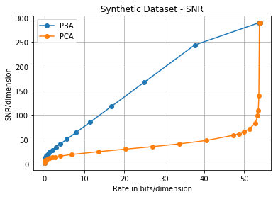
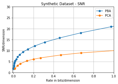
We evaluate the PBA compressor on MNIST [LBBH98], CIFAR-10 [Kri09], MIT Faces Dataset, Free Spoken Digit Dataset (FSDD) [Jac] and a synthetic Gaussian dataset. The synthetic Gaussian dataset is generated from a diagonal covariance matrix obtained from the eigenvalues of the Faces Dataset. We compare our algorithms primarily using mean-squared error since our theoretical analysis uses mean squared error as the distortion metric. Our plots display Signal-to-Noise ratios (SNRs) for ease of interpretation. For image datasets, we also compare our algorithms using the Structural Similarity (SSIM) or the Multi-scale Strctural Similarity (MS-SSIM) metrics when applicable [WBSS04]. We also consider errors on downstream tasks, specifically classification, as a distortion measure.

For all datasets, we compare the performance of the PBA compressor against baseline scheme derived from PCA that uses QCDsubscript𝑄𝐶𝐷Q_{CD} and QCDsuperscriptsubscript𝑄𝐶𝐷Q_{CD}^{\prime}. The PCA-based scheme sends some of the principal components essentially losslessly, and no information about the others. Specifically, in the context of our framework, for any given k𝑘k, we choose the first k𝑘k columns of 𝑾𝑾\bm{W} to be aligned with the first k𝑘k principal components of the dataset; the remaining columns are zero. Each nonzero column is scaled such that its Euclidean length multiplied by the eigenvalue has all the significant digits. This is done so that at high rates, the quantization procedure sends the k𝑘k principal components losslessly. The quantization and decoder operations are as in the PBA-based scheme; in particular the a2superscript𝑎2a^{2} parameter is as specified above. By varying k𝑘k, we trade off rate and distortion.

5.1 SNR Performance
Refer to caption
Refer to caption
Refer to caption
Refer to caption
Refer to caption
Refer to caption
Refer to caption
Refer to caption
Refer to caption
Refer to caption
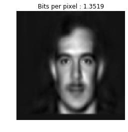
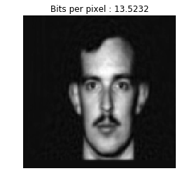
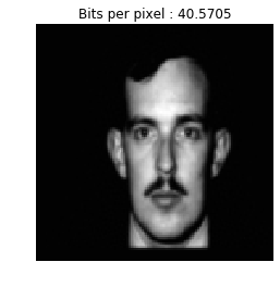
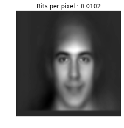
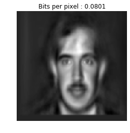
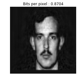
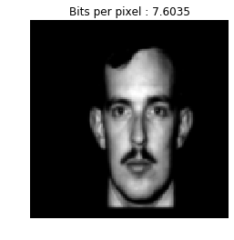
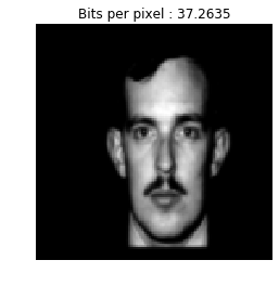
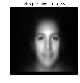
Figure 2: Reconstructions at different bits/pixel values for PCA (top) and PBA (bottom)
Refer to caption
Refer to caption
Refer to caption
Refer to caption
Refer to caption
Refer to caption
Refer to caption
Refer to caption
Figure 3: SNR/pixel vs Rate (bits/pixel) for MNIST, CIFAR-10, Faces, FSDD datasets. Figures in the bottom row are zoomed-in.
Refer to caption
Refer to caption
Refer to caption
Refer to caption
Refer to caption
Refer to caption
Refer to caption
Refer to caption
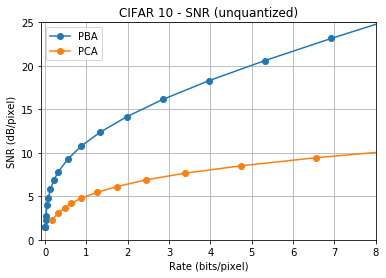
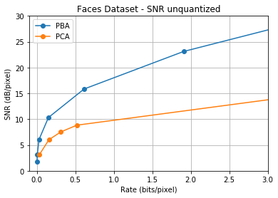
Figure 4: SNR/pixel vs Rate (bits/pixel) for MNIST, CIFAR-10, Faces and Synthetic dataset. Reconstructions are not rounded to integers from 00 to 255255255. The bottom four plots are zoomed-in versions of the top four plots.
Refer to caption
Refer to caption
Refer to caption
Refer to caption
Refer to caption
Refer to caption
Refer to caption
Refer to caption
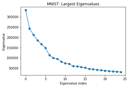
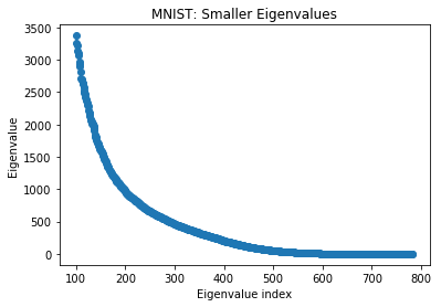
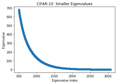
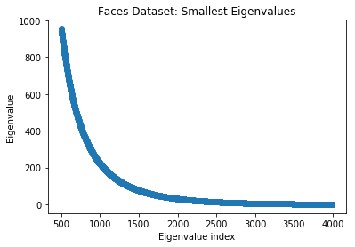
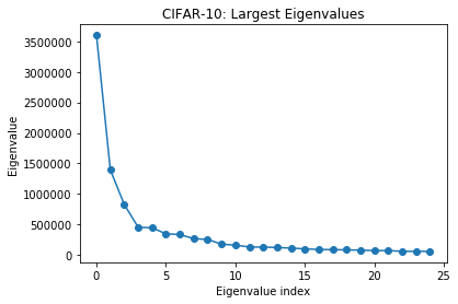
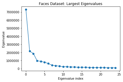
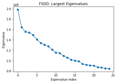
Figure 5: Eigenvalue distribution of the datasets. The top three plots are the largest 25 eigenvalues for MNIST, CIFAR-10, Faces and FSDD dataset. The bottom four figures plot the remaining eigenvalues except the largest 500.
Refer to caption
Refer to caption
Refer to caption
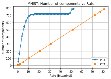
Figure 6: Plots of number of components sent vs rate (bits/pixel) for PBA and PCA.

We begin by examining compression performance under mean squared error, or equivalently, the SNR, defined as

SNR=10log10(PMSE).SNR10subscript10𝑃MSE\text{SNR}=10\cdot\log_{10}\left(\frac{P}{\text{MSE}}\right).

where P𝑃P is the empirical second moment of the dataset. This was the objective that PBA (and PCA) is designed to minimize.

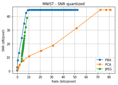
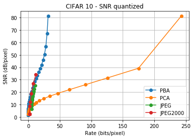
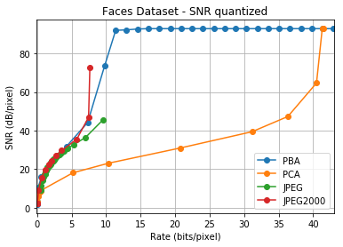
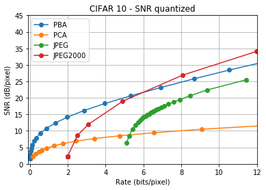
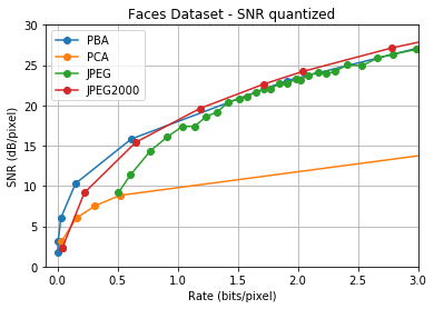
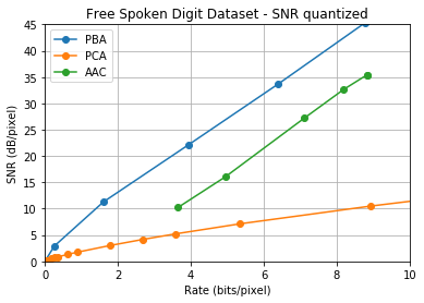
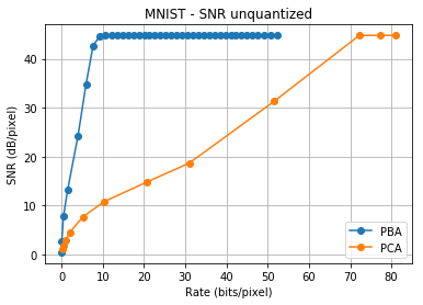
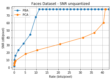
In Figure 2, we display reconstructions for a particular image in the Faces Dataset under PBA and PCA. Figure 3 shows the tradeoff for PBA and PCA against JPEG and JPEG2000 (for the image datasets) and AAC (for the audio dataset). All of the image datasets have integer pixel values between 0 and 255. Accordingly, we round the reconstuctions of PBA and PCA to the nearest integer in this range. Figure 4 shows the same tradeoff for PBA and PCA when reconstructions are not rounded off to the nearest integer. We see that PBA consistently outperforms PCA and JPEG, and is competitive with JPEG2000, even though the JPEG and JPEG2000 are variable-rate. 444It should be noted, however, that JPEG and JPEG2000 aim to minimize subjective distortion, not MSE, and they do not allow for training on sample images, as PBA and PCA do. A similar caveat applies to AAC. We estimate the size of the JPEG header by compressing an empty image and subtract this estimate from all the compression sizes produced by JPEG. We do not plot JPEG2000 performance for MNIST since it requires at least a 32x32 image. For audio data, we observe that PBA consistently outperforms PCA and AAC. Since the image data all use 888 bits per pixel, one can obtain infinite SNR at this rate via the trivial encoding that communicates the raw bits. PCA and PBA do not find this solution because they quantize in the transform domain, where the lattice-nature of the pixel distribution is not apparent. Determining how to leverage lattice structure in the source distribution for purposes of compression is an interesting question that transcends the PBA and PCA algorithms and that we will not pursue here.

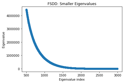
The reason that PCA performs poorly is that it favors sending the less significant bits of the most significant components over the most significant bits of less significant components, when the latter are more valuable for reconstructing the source. Arguably, it does not identify the “principal bits.” Figure 5 shows the eigenvalue distribution of the different datasets, and Figure 6 shows the number of distinct components about which information is sent as a function of rate for both PBA and PCA. We see that PBA sends information about many more components for a given rate than does PCA. We discuss the ramifications of this for downstream tasks, such as classification, in Section 5.3.

5.2 SSIM Performance
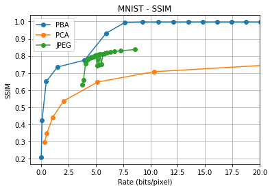
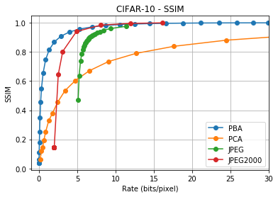
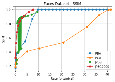
Structural similarity (SSIM) and Multi-Scale Structural similarity (MS-SSIM) are metrics that are tuned to perceptual similarity. Given two images, the SSIM metric outputs a real value between 00 and 111 where a higher value indicates more similarity between the images. We evaluate the performance of our algorithms on these metrics as well in Figure 7. We see that PBA consistently dominates PCA, and although it was not optimized for this metric, beats JPEG at low rates as well.

Refer to caption
Refer to caption
Refer to caption
Figure 7: SSIM vs Rate (bits/pixel) for MNIST, CIFAR-10, Faces Dataset

5.3 Performance on Downstream tasks
Lastly, we compare the impact of using PBA and PCA on an important downstream task, namely classification. We evaluate the algorithms on MNIST and CIFAR-10 datasets and use neural networks for classification. Our hyperparameter and architecture choices are given in Table 1. We divide the dataset into three parts. From the first part, we obain the covariance matrix that we use for PCA and to obtain the PBA compressor. The second and third part are used as training and testing data for the purpose of classification. For a fixed rate, reconstructions are passed to the neural networks for training and testing respectively. Since our goal is to compare classification accuracy across the compressors, we fix both the architecture and hyperparameters, and do not perform any additional tuning for the separate algorithms.

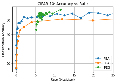
Figure 8 shows that PBA outperforms PCA in terms of accuracy. The difference is especially significant for low rates; all algorithms attain roughly the same performance at higher rates.
Hyperparameter MNIST CIFAR-10
Architecture 2-layer fully connected NN Convolutional Neural Network
with 2 convolutional layers, pooling and
three fully connected layers
# Hidden Neurons 100 NA
Optimization Algorithm Adam SGD with momentum
Loss Cross-entropy Cross-entropy
Learning Rate 0.0005 0.01
Table 1: Hyperparameter Choices and Architecture for Classification
Refer to caption
Refer to caption
Figure 8: Accuracy vs Rate (bits/pixel) for MNIST, CIFAR-10

References

  • [AMT+17] Eirikur Agustsson, Fabian Mentzer, Michael Tschannen, Lukas Cavigelli, Radu Timofte, Luca Benini, and Luc V Gool. Soft-to-hard vector quantization for end-to-end learning compressible representations. In Advances in Neural Information Processing Systems 30, pages 1141–1151, 2017.
  • [AT20] Eirikur Agustsson and Lucas Theis. Universally quantized neural compression. In Advances in Neural Information Processing Systems 33, pages 12367–12376, 2020.
  • [ATM+19] Eirikur Agustsson, Michael Tschannen, Fabian Mentzer, Radu Timofte, and Luc Van Gool. Generative adversarial networks for extreme learned image compression. In Proceedings of the IEEE International Conference on Computer Vision, pages 221–231, 2019.
  • [BCM+20] Johannes Ballé, Philip A Chou, David Minnen, Saurabh Singh, Nick Johnston, Eirikur Agustsson, Sung Jin Hwang, and George Toderici. Nonlinear transform coding. arXiv:2007.03034, 2020.
  • [Ber99] Dimitri P. Bertsekas. Nonlinear Programming. Athena Scientific, 1999.
  • [BH89] Pierre Baldi and Kurt Hornik. Neural networks and principal component analysis: Learning from examples without local minima. Neural Networks, 2(1):53 – 58, 1989.
  • [Bis06] Christopher M. Bishop. Pattern Recognition and Machine Learning (Information Science and Statistics). Springer-Verlag, Berlin, Heidelberg, 2006.
  • [BK88] Herve Bourlard and Y. Kamp. Auto-association by multilayer perceptrons and singular value decomposition. Biological Cybernetics, 59:291–294, 1988.
  • [Bla65] Nelson M. Blachman. The convolution inequality for entropy powers. IEEE Trans. Inf. Theory, 11(2):267–271, April 1965.
  • [BLS16] Johannes Ballé, Valero Laparra, and Eero Simoncelli. End-to-end optimization of nonlinear transform codes for perceptual quality. In 2016 Picture Coding Symposium (PCS), 2016.
  • [BLSG20] Xuchan Bao, James Lucas, Sushant Sachdeva, and Roger Grosse. Regularized linear autoencoders recover the principal components, eventually. arXiv:2007.06731, 2020.
  • [BMS+18] Johannes Ballé, David Minnen, Saurabh Singh, Sung Jin Hwang, and Nick Johnston. Variational image compression with a scale hyperprior. In International Conference on Learning Representations, 2018.
  • [BV04] Stephen Boyd and Lieven Vandenberghe. Convex Optimization. Cambridge, 2004.
  • [CEKL19] Yoojin Choi, Mostafa El-Khamy, and Jungwon Lee. Variable rate deep image compression with a conditional autoencoder. In Proceedings of the IEEE/CVF International Conference on Computer Vision (ICCV), October 2019.
  • [CT06] Thomas M. Cover and Joy A. Thomas. Elements of Information Theory. Wiley, 2006.
  • [HJ13] Roger A. Horn and Charles R. Johnson, editors. Matrix Analysis. Cambridge University Press, USA, 2013.
  • [HRTC19] Amirhossein Habibian, Ties van Rozendaal, Jakub M Tomczak, and Taco S Cohen. Video compression with rate-distortion autoencoders. In Proceedings of the IEEE International Conference on Computer Vision, pages 7033–7042, 2019.
  • [HS06] Geoffrey E Hinton and Ruslan R Salakhutdinov. Reducing the dimensionality of data with neural networks. Science, 313(5786):504–507, 2006.
  • [Jac] Zohar Jackson. Free spoken digit dataset (fsdd). https://github.com/Jakobovski/free-spoken-digit-dataset.
  • [Kay98] Steven M Kay. Estimation Theory. Prentice Hall PTR, 1998.
  • [KBGS19] Daniel Kunin, Jonathan Bloom, Aleksandrina Goeva, and Cotton Seed. Loss landscapes of regularized linear autoencoders. In International Conference on Machine Learning, volume 97, pages 3560–3569, 2019.
  • [Kri09] Alex Krizhevsky. Learning multiple layers of features from tiny images. Master’s Thesis, Department of Computer Science, University of Toronto, 2009.
  • [LBBH98] Yann LeCun, Léon Bottou, Yoshua Bengio, and Patrick Haffner. Gradient-based learning applied to document recognition. Proceedings of the IEEE, 86(11):2278–2324, 1998.
  • [LNP19] Saïd Ladjal, Alasdair Newson, and Chi-Hieu Pham. A pca-like autoencoder. abs/1904.01277, 2019.
  • [LTGN19] James Lucas, George Tucker, Roger B Grosse, and Mohammad Norouzi. Don’t blame the elbo! a linear vae perspective on posterior collapse. In Advances in Neural Information Processing Systems, volume 32, pages 9408–9418, 2019.
  • [LZW+21] Liang Liao, Xuechun Zhang, Xinqiang Wang, Sen Lin, and Xin Liu. Generalized image reconstruction over t-algebra. arXiv:2101.06650, 2021.
  • [MB95] Alan V. McCree and Thomas P. Barnwell. A mixed excitation lpc vocoder model for low bit rate speech coding. IEEE Transactions on Speech and Audio Processing, 3(4):242–250, 1995.
  • [MOA11] Albert W. Marshall, Ingram Olkin, and Barry C. Arnold. Inequalities: Theory of Majorization and its Applications, volume 143. Springer, 2011.
  • [OSWS20] Reza Oftadeh, Jiayi Shen, Zhangyang Wang, and Dylan Shell. Eliminating the invariance on the loss landscape of linear autoencoders. In International Conference on Machine Learning, pages 7405–7413, 2020.
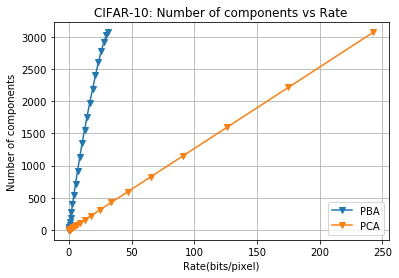
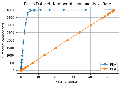
  • [RB17] Oren Rippel and Lubomir Bourdev. Real-time adaptive image compression. In International Conference on Machine Learning, pages 2922–2930, 2017.
  • [RZM19] Michal Rolínek, Dominik Zietlow, and Georg Martius. Variational autoencoders pursue pca directions (by accident). In Proceedings of the IEEE/CVF Conference on Computer Vision and Pattern Recognition (CVPR), June 2019.
  • [SA85] M. Schroeder and B. Atal. Code-excited linear prediction(celp): High-quality speech at very low bit rates. In IEEE International Conference on Acoustics, Speech, and Signal Processing, volume 10, pages 937–940, 1985.
  • [San12] Rafael do EspArito Santo. Principal Component Analysis Applied to Digital Image Compression. Einstein (Sáo Paulo), 10:135 – 139, 06 2012.
  • [TAL18] Michael Tschannen, Eirikur Agustsson, and Mario Lucic. Deep generative models for distribution-preserving lossy compression. In Advances in Neural Information Processing Systems 31, pages 5929–5940. 2018.
  • [TOH+16] George Toderici, Sean M O’Malley, Sung Jin Hwang, Damien Vincent, David Minnen, Shumeet Baluja, Michele Covell, and Rahul Sukthankar. Variable rate image compression with recurrent neural networks. In International Conference on Learning Representations, 2016.
  • [TSCH17] Lucas Theis, Wenzhe Shi, Andrew Cunningham, and Ferenc Huszár. Lossy image compression with compressive autoencoders. In International Conference on Learning Reperesentations, 2017.
  • [TVJ+17] George Toderici, Damien Vincent, Nick Johnston, Sung Jin Hwang, David Minnen, Joel Shor, and Michele Covell. Full resolution image compression with recurrent neural networks. In IEEE Conference on Computer Vision and Pattern Recognition, pages 5435–5443, 2017.
  • [Vor] Vorbis audio compression. https://xiph.org/vorbis/. Accessed: 2021-01-26.
  • [WBSS04] Zhou Wang, A. C Bovik, H. R. Sheikh, and E. P. Simoncelli. Image quality assessment: From error visibility to structural similarity. IEEE Transactions on Image Processing, 13(4):600–612, 2004.
  • [ZCG+18] Lei Zhou, Chunlei Cai, Yue Gao, Sanbao Su, and Junmin Wu. Variational autoencoder for low bit-rate image compression. In Proceedings of the IEEE Conference on Computer Vision and Pattern Recognition Workshops, pages 2617–2620, 2018.
  • [ZF92] Ram Zamir and Meir Feder. On universal quantization by randomized uniform/lattice quantizers. IEEE Trans. Inf. Theory, 38:428–436, 1992.

Appendix A Review of Schur-Convexity

In this section, we review the key definitions and theorems related to Schur-convexity that we use in the proof of Theorem 1.

Definition 7.

(Majorization)[HJ13] For a vector 𝐯d𝐯superscript𝑑\bm{v}\in\mathbb{R}^{d}, let 𝐯superscript𝐯\bm{v}^{\downarrow} denote the vector with the same components arranged in descending order. Given vectors 𝐚,𝐛d𝐚𝐛superscript𝑑\bm{a},\bm{b}\in\mathbb{R}^{d}, we say 𝐚𝐚\bm{a} majorizes 𝐛𝐛\bm{b} and denote 𝐚𝐛succeeds𝐚𝐛\bm{a}\succ\bm{b}, if

i=1d[𝒂]i=i=1d[𝒃]i,superscriptsubscript𝑖1𝑑subscriptdelimited-[]𝒂𝑖superscriptsubscript𝑖1𝑑subscriptdelimited-[]𝒃𝑖\sum\limits_{i=1}^{d}\left[\bm{a}\right]_{i}=\sum\limits_{i=1}^{d}\left[\bm{b}\right]_{i},

and for all k[d1]𝑘delimited-[]𝑑1k\in\left[d-1\right],

i=1k[𝒂]ii=1k[𝒃]i.superscriptsubscript𝑖1𝑘subscriptdelimited-[]superscript𝒂𝑖superscriptsubscript𝑖1𝑘subscriptdelimited-[]superscript𝒃𝑖\sum\limits_{i=1}^{k}\left[\bm{a}^{\downarrow}\right]_{i}\geq\sum\limits_{i=1}^{k}\left[\bm{b}^{\downarrow}\right]_{i}.
Definition 8.

(Schur-convexity) A function f:d:𝑓superscript𝑑f:\mathbb{R}^{d}\rightarrow\mathbb{R} is Schur-convex if for any vectors 𝐚,𝐛d𝐚𝐛superscript𝑑\bm{a},\bm{b}\in\mathbb{R}^{d}, such that 𝐚𝐛succeeds𝐚𝐛\bm{a}\succ\bm{b},

f(𝒂)f(𝒃).𝑓𝒂𝑓𝒃f\left(\bm{a}\right)\geq f\left(\bm{b}\right).

f𝑓f is strictly Schur-convex if the above inequality is a strict inequality for any 𝐚𝐛succeeds𝐚𝐛\bm{a}\succ\bm{b} that are not permutations of each other. f𝑓f is Schur-concave if the direction of the inequality is reversed and is strictly Schur concave if the direction of the inequality is reversed and it is a strict inequality for any 𝐚𝐛succeeds𝐚𝐛\bm{a}\succ\bm{b} that are not permutations of each other.

Proposition 9.

[MOA11] If f::𝑓f:\mathbb{R}\rightarrow\mathbb{R} is convex, then ϕ:d:italic-ϕsuperscript𝑑\phi:\mathbb{R}^{d}\rightarrow\mathbb{R} given by

ϕ(𝒗)=i=1df([v]i)italic-ϕ𝒗superscriptsubscript𝑖1𝑑𝑓subscriptdelimited-[]𝑣𝑖\phi\left(\bm{v}\right)=\sum\limits_{i=1}^{d}f\left(\left[v\right]_{i}\right)

is Schur-convex. If f𝑓f is concave, then ϕitalic-ϕ\phi is Schur-concave. Likewise if f𝑓f is strictly convex, ϕitalic-ϕ\phi is strictly Schur-convex and if f𝑓f is strictly concave, ϕitalic-ϕ\phi is strictly Schur-concave.