Heuristic-Guided Reinforcement Learning

Abstract

We provide a framework for accelerating reinforcement learning (RL) algorithms by heuristics constructed from domain knowledge or offline data. Tabula rasa RL algorithms require environment interactions or computation that scales with the horizon of the sequential decision-making task. Using our framework, we show how heuristic-guided RL induces a much shorter-horizon subproblem that provably solves the original task. Our framework can be viewed as a horizon-based regularization for controlling bias and variance in RL under a finite interaction budget. On the theoretical side, we characterize properties of a good heuristic and its impact on RL acceleration. In particular, we introduce the novel concept of an improvable heuristic, a heuristic that allows an RL agent to extrapolate beyond its prior knowledge. On the empirical side, we instantiate our framework to accelerate several state-of-the-art algorithms in simulated robotic control tasks and procedurally generated games. Our framework complements the rich literature on warm-starting RL with expert demonstrations or exploratory datasets, and introduces a principled method for injecting prior knowledge into RL.

1 Introduction

Many recent empirical successes of reinforcement learning (RL) require solving problems with very long decision-making horizons. OpenAI Five [1] used episodes that were $20000$ timesteps on average, while AlphaStar [2] used roughly $5000$ timesteps. Long-term credit assignment is a very challenging statistical problem, with the sample complexity growing quadratically (or worse) with the horizon [3]. Long horizons (or, equivalently, large discount factors) also increase RL’s computational burden, leading to slow optimization convergence [4]. This makes RL algorithms require prohibitively large amounts of interactions and compute: even with tuned hyperparameters, AlphaStar needed over $10^{8}$ samples and OpenAI Five needed over $10^{7}$ PFLOPS of compute.

A popular approach to mitigate the statistical and computational issues of tabula rasa RL methods is to warm-start or regularize learning with prior knowledge [5, 6, 7, 8, 2, 1, 9, 10]. For instance, AlphaStar learned a policy and value function from human demonstrations and regularized the RL agent using imitation learning (IL). AWAC [9] warm-started a policy using batch policy optimization on exploratory datasets. While these approaches have been effective in different domains, none of them explicitly address RL’s complexity dependence on horizon.

In this paper, we propose a complementary regularization technique that relies on heuristic value functions, or heuristics for short, to effectively shorten the problem horizon faced by an online RL agent for fast learning. We call this approach Heuristic-Guided Reinforcement Learning (HuRL). The core idea is simple: given a Markov decision process (MDP) $\mathcal{M}=(\SS,\mathcal{A},P,r,\gamma)$ and a heuristic $h:\SS\to\mathbb{R}$, we select a mixing coefficient $\lambda\in[0,1]$ and have the agent solve a new MDP $\widetilde{\mathcal{M}}=(\SS,\mathcal{A},P,\widetilde{r},\widetilde{\gamma})$ with a reshaped reward and a smaller discount (i.e. a shorter horizon):

$$\widetilde{r}(s,a)\coloneqq r(s,a)+(1-\lambda)\gamma\mathbb{E}_{s^{\prime}\sim P(\cdot|s,a)}[h(s^{\prime})]\quad\text{and}\quad\widetilde{\gamma}\coloneqq\lambda\gamma.$$ (1)

HuRL effectively introduces horizon-based regularization that determines whether long-term value information should come from collected experiences or the heuristic. By modulating the effective horizon via $\lambda$, we trade off the bias and the complexity of solving the reshaped MDP. HuRL with $\lambda=1$ recovers the original problem and with $\lambda=0$ creates an easier contextual bandit problem [12].

A heuristic $h$ in HuRL represents a prior guess of the desired long-term return of states, which ideally is the optimal value function $V^{*}$ of the unknown MDP $\mathcal{M}$. When the heuristic $h$ captures the state ordering of $V^{*}$ well, conceptually, it becomes possible to make good long-term decisions by short-horizon planning or even acting greedily. How do we construct a good heuristic? In the planning literature, this is typically achieved by solving a relaxation of the original problem [13, 14, 15]. Alternatively, one can learn it from batch data collected by exploratory behavioral policies (as in offline RL [16]) or from expert policies (as in IL [17]). For some dense reward problems, a zero heuristic can be effective in reducing RL complexity, as exploited by the guidance discount framework [18, 19, 20, 21, 22, 23]. In this paper, we view heuristics as a unified representation of various forms of prior knowledge, such as expert demonstrations, exploratory datasets, and engineered guidance.

Although the use of heuristics to accelerate search has been popular in planning and control algorithms, e.g., A* [24], MCTS [25], and MPC [26, 7, 27, 28], its theory is less developed for settings where the MDP is unknown. The closest work in RL is potential-based reward shaping (PBRS) [29], which reshapes the reward into $\bar{r}(s,a)=r(s,a)+\gamma\mathbb{E}_{s^{\prime}|s,a}[h(s^{\prime})]-h(s)$ while keeping the original discount. PBRS can use any heuristic to reshape the reward while preserving the ordering of policies. However, giving PBRS rewards to an RL algorithm does not necessarily lead to faster learning, because the base RL algorithm would still seek to explore to resolve long-term credit assignment. HuRL allows common RL algorithms to leverage the short-horizon potential provided by a heuristic to learn faster.

In this work, we provide a theoretical foundation of HuRL to enable adopting heuristics and horizon reduction for accelerating RL, combining advances from the PBRS and the guidance discount literatures. On the theoretical side, we derive a bias-variance decomposition of HuRL’s horizon-based regularization in order to characterize the solution quality as a function of $\lambda$ and $h$. Using this insight, we provide sufficient conditions for achieving an effective trade-off, including properties required of a base RL algorithm that solves the reshaped MDP $\widetilde{\mathcal{M}}_{\lambda}$. Furthermore, we define the novel concept of an improvable heuristic and prove that good heuristics for HuRL can be constructed from data using existing pessimistic offline RL algorithms (such as pessimistic value iteration [30, 31]).

The effectiveness of HuRL depends on the heuristic quality, so we design HuRL to employ a sequence of mixing coefficients (i.e. $\lambda$s) that increases as the agent gathers more data from the environment. Such a strategy induces a learning curriculum that enables HuRL to remain robust to non-ideal heuristics. HuRL starts off by guiding the agent’s search direction with a heuristic. As the agent becomes more experienced, it gradually removes the guidance and lets the agent directly optimize the true long-term return. We empirically validate HuRL in MuJoCo [32] robotics control problems and Procgen games [33] with various heuristics and base RL algorithms. The experimental results demonstrate the versatility and effectiveness of HuRL in accelerating RL algorithms.

2 Preliminaries

2.1 Notation

We focus on discounted infinite-horizon Markov Decision Processes (MDPs) for ease of exposition. The technique proposed here can be extended to other MDP settings. A discounted infinite-horizon MDP is denoted as a 5-tuple $\mathcal{M}=(\SS,\mathcal{A},P,r,\gamma)$, where $\SS$ is the state space, $\mathcal{A}$ is the action space, $P(s^{\prime}|s,a)$ is the transition dynamics, $r(s,a)$ is the reward function, and $\gamma\in[0,1)$ is the discount factor. Without loss of generality, we assume $r:\SS\times\mathcal{A}\to[0,1]$. We allow the state and action spaces $\SS$ and $\mathcal{A}$ to be either discrete or continuous. Let $\Delta(\cdot)$ denote the space of probability distributions. A decision-making policy $\pi$ is a conditional distribution $\pi:\SS\to\Delta(\mathcal{A})$, which can be deterministic. We define some shorthand for writing expectations: For a state distribution $d\in\Delta(\SS)$ and a function ${V:\SS\to\mathbb{R}}$, we define $V(d)\coloneqq\mathbb{E}_{s\sim d}[V(s)]$; similarly, for a policy $\pi$ and a function $Q:\SS\times\mathcal{A}\to\mathbb{R}$, we define ${Q(s,\pi)\coloneqq\mathbb{E}_{a\sim\pi(\cdot|s)}[Q(s,a)]}$. Lastly, we define $\mathbb{E}_{s^{\prime}|s,a}\coloneqq\mathbb{E}_{s^{\prime}\sim P(\cdot|s,a)}$.

Central to solving MDPs are the concepts of value functions and average distributions. For a policy $\pi$, we define its state value function $V^{\pi}$ as $V^{\pi}(s)\coloneqq\mathbb{E}_{\rho_{s}^{\pi}}\left[\sum_{t=0}^{\infty}\gamma^{t}r(s_{t},a_{t})\right],$ where $\rho_{s}^{\pi}$ denotes the trajectory distribution of $s_{0},a_{0},s_{1},\dots$ induced by running $\pi$ starting from $s_{0}=s$. We define the state-action value function (or the Q-function) as $Q^{\pi}(s,a)\coloneqq r(s,a)+\gamma\mathbb{E}_{s^{\prime}|s,a}[V^{\pi}(s^{\prime})]$. We denote the optimal policy as $\pi^{*}$ and its state value function as $V^{*}\coloneqq V^{\pi^{*}}$. Under the assumption that rewards are in $[0,1]$, we have $V^{\pi}(s),Q^{\pi}(s,a)\in[0,\frac{1}{1-\gamma}]$ for all $\pi$, $s\in\SS$, and $a\in\mathcal{A}$. We denote the initial state distribution of interest as $d_{0}\in\Delta(\SS)$ and the state distribution of policy $\pi$ at time $t$ as $d_{t}^{\pi}$, with $d_{0}^{\pi}=d_{0}$. Given $d_{0}$, we define the average state distribution of a policy $\pi$ as $d^{\pi}\coloneqq(1-\gamma)\sum_{t=0}^{\infty}\gamma^{t}d_{t}^{\pi}$. With a slight abuse of notation, we also write $d^{\pi}(s,a)\coloneqq d^{\pi}(s)\pi(a|s)$.

2.2 Setup: Reinforcement Learning with Heuristics

We consider RL with prior knowledge expressed in the form of a heuristic value function. The goal is to find a policy $\pi$ that has high return through interactions with an unknown MDP $\mathcal{M}$, i.e., $\max_{\pi}V^{\pi}(d_{0})$. While the agent here does not fully know $\mathcal{M}$, we suppose that, before interactions start the agent is provided with a heuristic $h:\SS\to\mathbb{R}$ which the agent can query throughout learning.

The heuristic $h$ represents a prior guess of the optimal value function $V^{*}$ of $\mathcal{M}$. Common sources of heuristics are domain knowledge as typically employed in planning, and logged data collected by exploratory or by expert behavioral policies. In the latter, a heuristic guess of $V^{*}$ can be computed from the data by offline RL algorithms. For instance, when we have trajectories of an expert behavioral policy, Monte-Carlo regression estimate of the observed returns may be a good guess of $V^{*}$.

Using heuristics to solve MDP problems has been popular in planning and control, but its usage is rather limited in RL. The closest provable technique in RL is PBRS [29], where the reward is modified into $\overline{r}(s,a)\coloneqq r(s,a)+\gamma\mathbb{E}_{s^{\prime}|s,a}[h(s^{\prime})]-h(s)$. It can be shown that this transformation does not introduce bias into the policy ordering, and therefore solving the new MDP $\overline{\mathcal{M}}\coloneqq(\SS,\mathcal{A},P,\overline{r},\gamma)$ would yield the same optimal policy $\pi^{*}$ of $\mathcal{M}$.

Conceptually when the heuristic is the optimal value function $h=V^{*}$, the agent should be able to find the optimal policy $\pi^{*}$ of $\mathcal{M}$ by acting myopically, as $V^{*}$ already contains all necessary long-term information for good decision making. However, running an RL algorithm with the PBRS reward (i.e. solving $\overline{\mathcal{M}}\coloneqq(\SS,\mathcal{A},P,\overline{r},\gamma)$) does not take advantage of this shortcut. To make learning efficient, we need to also let the base RL algorithm know that acting greedily (i.e., using a smaller discount) with the shaped reward can yield good policies. An intuitive idea is to run the RL algorithm to maximize $\overline{V}^{\pi}_{\lambda}(d_{0})$, where $\overline{V}^{\pi}_{\lambda}$ denotes the value function of $\pi$ in an MDP $\overline{\mathcal{M}}_{\lambda}\coloneqq(\SS,\mathcal{A},P,\overline{r},\lambda\gamma)$ for some $\lambda\in[0,1]$. However this does not always work. For example, when $\lambda=0$, $\max_{\pi}\overline{V}^{\pi}_{\lambda}(d_{0})$ only optimizes for the initial states $d_{0}$, but obviously the agent is going to encounter other states in $\mathcal{M}$. We next propose a provably correct version, HuRL, to leverage this short-horizon insight.

3 Heuristic-Guided Reinforcement Learning

We propose a general framework, HuRL, for leveraging heuristics to accelerate RL. In contrast to tabula rasa RL algorithms that attempt to directly solve the long-horizon MDP $\mathcal{M}$, HuRL uses a heuristic to guide the agent in solving a sequence of short-horizon MDPs so as to amortize the complexity of long-term credit assignment. In effect, HuRL creates a heuristic-based learning curriculum to help the agent learn faster.

3.1 Algorithm

HuRL takes a reduction-based approach to realize the idea of heuristic guidance. As summarized in Algorithm 1, HuRL takes a heuristic $h:\SS\to\mathbb{R}$ and a base RL algorithm $\mathcal{L}$ as input, and outputs an approximately optimal policy for the original MDP $\mathcal{M}$. During training, HuRL iteratively runs the base algorithm $\mathcal{L}$ to collect data from the MDP $\mathcal{M}$ and then uses the heuristic $h$ to modify the agent’s collected experiences. Namely, in iteration $n$, the agent interacts with the original MDP $\mathcal{M}$ and saves the raw transition tuples $\mathcal{D}_{n}=\{(s,a,r,s^{\prime})\}$ (line 2). HuRL then defines a reshaped MDP $\widetilde{\mathcal{M}}_{n}\coloneqq(\SS,\mathcal{A},P,\widetilde{r}_{n},\widetilde{\gamma}_{n})$ (line 3) by changing the rewards and lowering the discount factor:

$$\widetilde{r}_{n}(s,a)\coloneqq r(s,a)+(1-\lambda_{n})\gamma\mathbb{E}_{s^{\prime}|s,a}[h(s^{\prime})]\qquad\text{and}\qquad\widetilde{\gamma}_{n}\coloneqq\lambda_{n}\gamma,$$ (2)

where $\lambda_{n}\in[0,1]$ is the mixing coefficient. The new discount $\widetilde{\gamma}_{n}$ effectively gives $\widetilde{\mathcal{M}}_{n}$ a shorter horizon than $\mathcal{M}$’s, while the heuristic $h$ is blended into the new reward in (2) to account for the missing long-term information. We call $\widetilde{\gamma}_{n}=\lambda_{n}\gamma$ in (2) the guidance discount to be consistent with prior literature [20], which can be viewed in terms of our framework as using a zero heuristic. In the last step (line 4), HuRL calls the base algorithm $\mathcal{L}$ to perform updates with respect to the reshaped MDP $\widetilde{\mathcal{M}}_{n}$. This is realized by 1) setting the discount factor used in $\mathcal{L}$ to $\widetilde{\gamma}_{n}$, and 2) setting the sampled reward to $r+(\gamma-\widetilde{\gamma}_{n})h(s^{\prime})$ for every transition tuple $(s,a,r,s^{\prime})$ collected from $\mathcal{M}$. We remark that the base algorithm $\mathcal{L}$ in line 2 always collects trajectories of lengths proportional to the original discount $\gamma$, while internally the optimization is done with a lower discount $\widetilde{\gamma}_{n}$ in line 4.

Over the course of training, HuRL repeats the above steps with a sequence of increasing mixing coefficients $\{\lambda_{n}\}$. From (2) we see that as the agent interacts with the environment, the effects of the heuristic in MDP reshaping decrease and the effective horizon of the reshaped MDP increases.

Algorithm 1 Heuristic-Guided Reinforcement Learning (HuRL)

0:  MDP $\mathcal{M}=(\SS,\mathcal{A},P,r,\gamma)$, RL algorithm $\mathcal{L}$, heuristic $h$, mixing coefficients $\{\lambda_{n}\}$.

1:  for $n=1,\dots,N$ do

2:     $\mathcal{D}_{n}\leftarrow\mathcal{L}$.CollectData($\mathcal{M}$)

3:     Get $\lambda_{n}$ from $\{\lambda_{n}\}$ and construct $\widetilde{\mathcal{M}}_{n}=(\SS,\mathcal{A},P,\widetilde{r}_{n},\widetilde{\gamma}_{n})$ according to (2) using $h$ and $\lambda_{n}$

4:     $\pi_{n}\leftarrow\mathcal{L}$.Train($\mathcal{D}_{n}$, $\widetilde{\mathcal{M}}_{n}$)

5:  end for

6:  return  $\pi_{N}$

3.2 HuRL as Horizon-based Regularization

We can think of HuRL as introducing a horizon-based regularization for RL, where the regularization center is defined by the heuristic and its strength diminishes as the mixing coefficient increases. As the agent collects more experiences, HuRL gradually removes the effects of regularization and the agent eventually optimizes for the original MDP.

HuRL’s regularization is designed to reduce learning variance, similar to the role of regularization in supervised learning. Unlike the typical weight decay imposed on function approximators (such as the agent’s policy or value networks), our proposed regularization leverages the structure of MDPs to regulate the complexity of the MDP the agent faces, which scales with the MDP’s discount factor (or, equivalently, the horizon). When the guidance discount $\widetilde{\gamma}_{n}$ is lower than the original discount $\gamma$ (i.e. $\lambda_{n}<1$), the reshaped MDP $\widetilde{\mathcal{M}}_{n}$ given by (2) has a shorter horizon and requires fewer samples to solve. However, the reduced complexity comes at the cost of bias, because the agent is now incentivized toward maximizing the performance with respect to the heuristic rather than the original long-term returns of $\mathcal{M}$. In the extreme case of $\lambda_{n}=0$, HuRL would solve a zero-horizon contextual bandit problem with contexts (i.e. states) sampled from $d^{\pi}$ of $\mathcal{M}$.

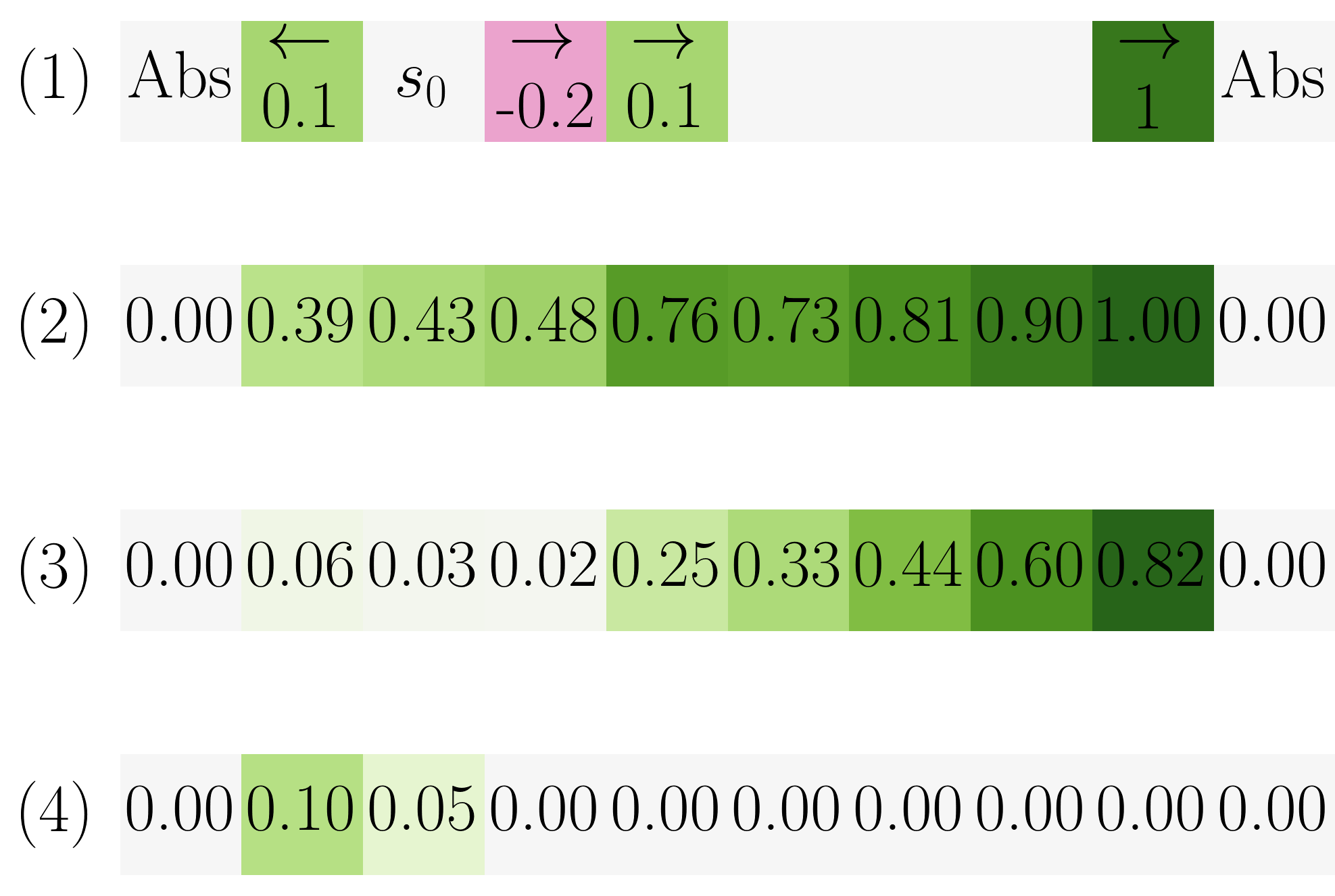
(a) Heatmap of different values.

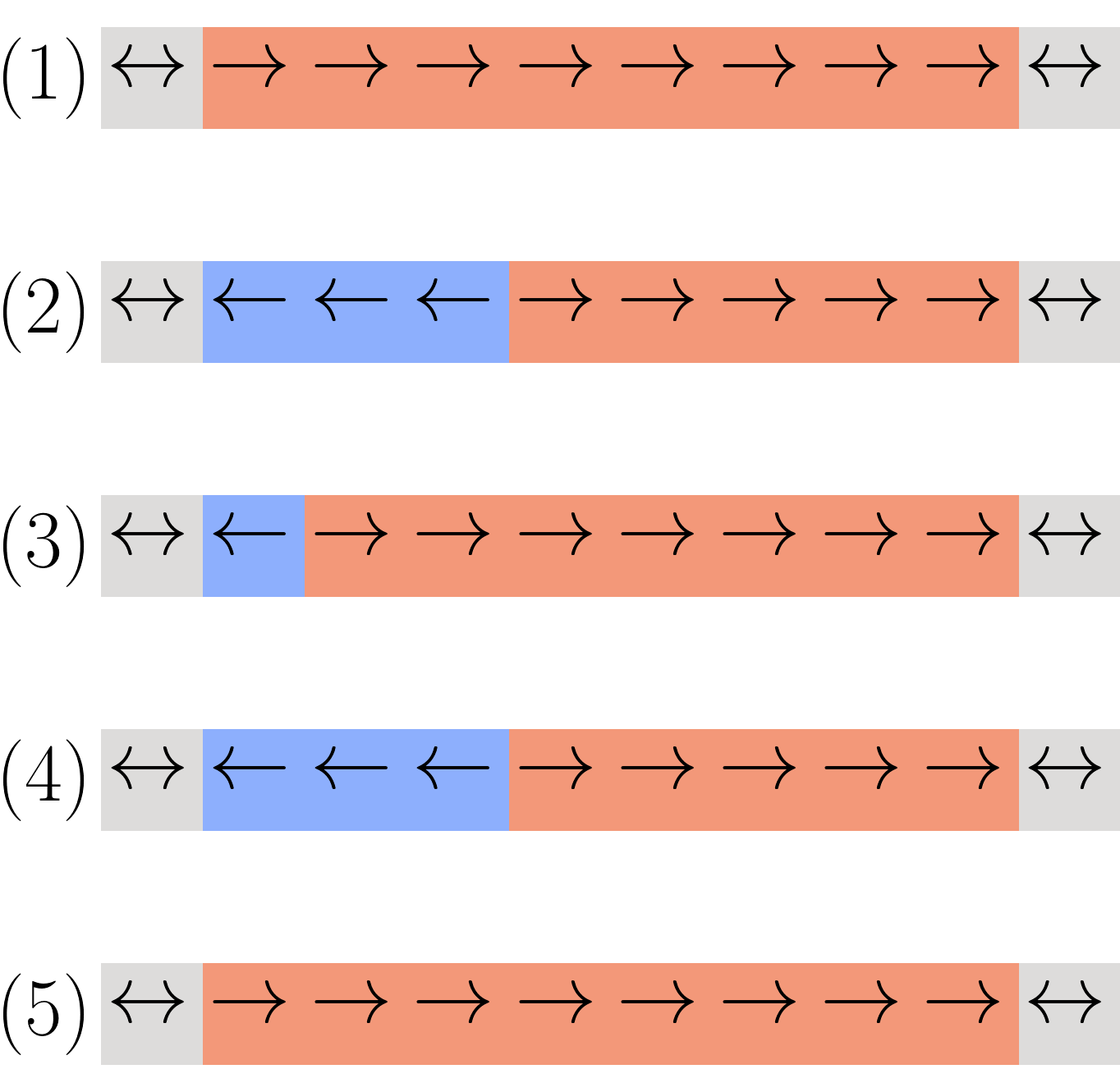
(b) Different policy behaviors.

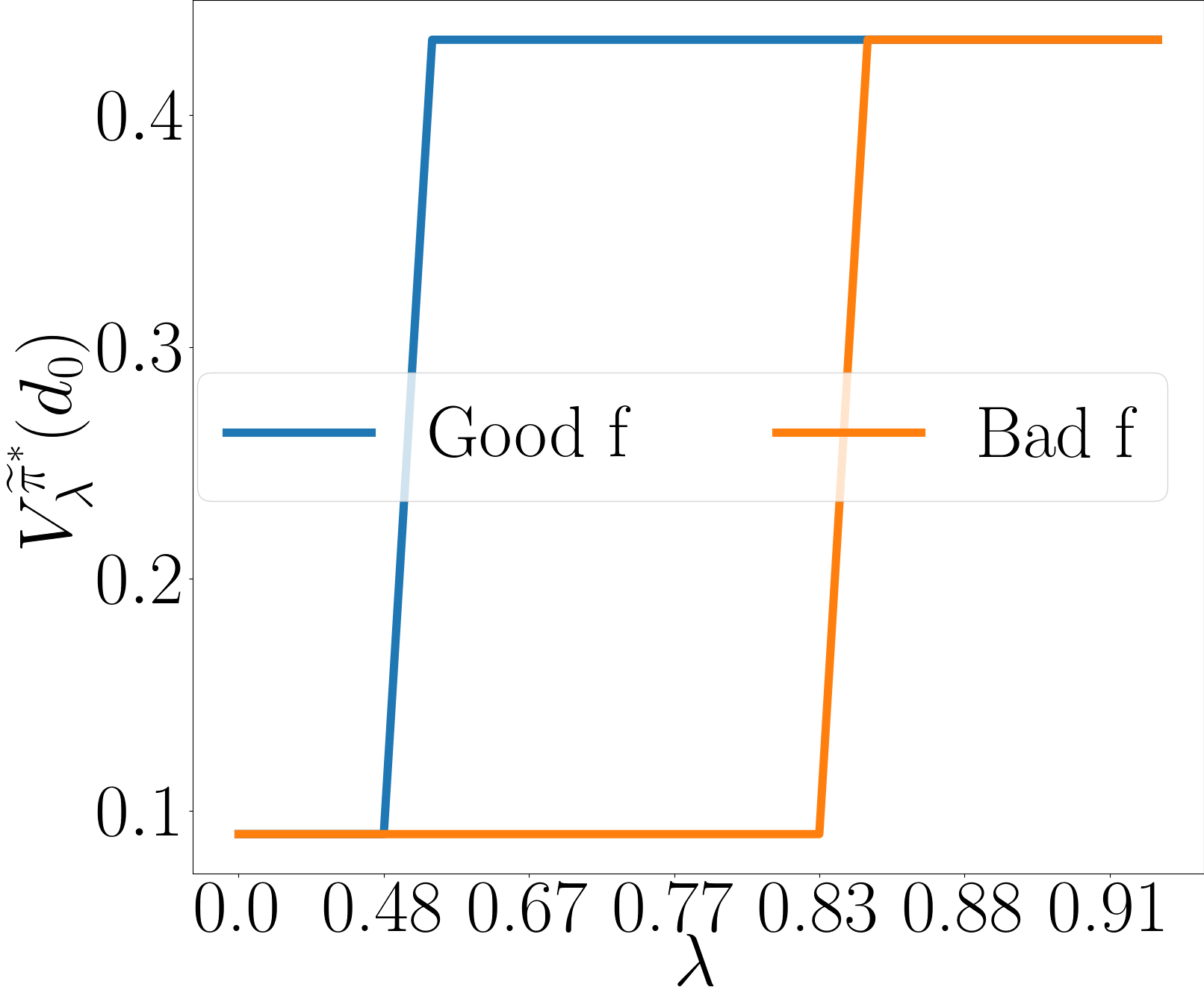
(c) HuRL with different $h$ and $\lambda$.

Figure 1: Example of HuRL in a chain MDP. Each cell in a row in each diagram represents a state from $\SS=\{1,\dots,10\}$. The agent starts at state $3$ ($s_{0}$), and states $1$ and $10$ are absorbing ($Abs$ in subfigure a-(1)). Actions $\mathcal{A}=\{\leftarrow,\rightarrow\}$ move the agent left or right in the chain unless the agent is in an absorbing state. Subfig. a-(1) shows the reward function: $r(2,\leftarrow)=0.1,r(4,\rightarrow)=-0.2,r(5,\rightarrow)=0.1$, and all state-action pairs not shown in a-(1) yield $r=0$. Subfig. a-(2) shows $V^{*}$ for $\gamma=0.9$. Subfig. a-(3) shows a good heuristic $h$ — $V(\text{random }\pi)$. Subfig. a-(4) shows a bad heuristic $h$ — $V(\text{myopic }\pi)$. Subfig. b-(1): $\pi^{*}$ for $V^{*}$ from a-(2). Subfig. b-(2): $\tilde{\pi}^{*}$ from HuRL with $h=0,\lambda=0.5$. Subfig. b-(3): $\tilde{\pi}^{*}$ from HuRL with the good $h$ from (a).(3) and $\lambda=0.5$. Subfig. b-(4): $\tilde{\pi}^{*}$ from the bad $h$ from a-(4), $\lambda=0.5$. Subfig. b-(5): $\tilde{\pi}^{*}$ from the bad $h$ and $\lambda=1$. Subfig. (c) illustrates the takeaway message: using HuRL with a good $h$ can find $\pi^{*}$ from $s_{0}$ even with a small $\lambda$ (see the $x$-axis), while HuRL with a bad $h$ requires a much higher $\lambda$ to discover $\pi^{*}$.

3.3 A Toy Example

We illustrate this idea in a chain MDP environment in Fig. 1. The optimal policy $\pi^{*}$ for this MDP’s original $\gamma=0.9$ always picks action $\rightarrow$, as shown in Fig. 1(b)-(1), giving the optimal value $V^{*}$ in Fig. 1(a)-(2). Suppose we used a smaller guidance discount $\widetilde{\gamma}=0.5\gamma$ to accelerate learning. This is equivalent to HuRL with a zero heuristic $h=0$ and $\lambda=0.5$. Solving this reshaped MDP yields a policy $\widetilde{\pi}^{*}$ that acts very myopically in the original MDP, as shown in Fig. 1(b)-(2); the value function of $\widetilde{\pi}^{*}$ in the original MDP is visualized in Fig. 1(a)-(4).

Now, suppose we use Fig. 1(a)-(4) as a heuristic in HuRL instead of $h=0$. This is a bad choice of heuristic (Bad $h$) as it introduces a large bias with respect to $V^{*}$ (cf. Fig. 1(a)-(2)). On the other hand, we can roll out a random policy in the original MDP and use its value function as the heuristic (Good $h$), shown in Fig. 1(a)-(3). Though the random policy has an even lower return at the initial state $s=3$, it gives a better heuristic because this heuristic shares the same trend as $V^{*}$ in Fig. 1(a)-(1). HuRL run with Good $h$ and Bad $h$ yields policies in Fig. 1(b)-(3,4), and the quality of the resulting solutions in the original MDP, $V_{\lambda}^{\widetilde{\pi}^{*}}(d_{0})$, is reported in Fig. 1(c) for different $\lambda$. Observe that HuRL with a good heuristic can achieve $V^{*}(d_{0})$ with a much smaller horizon $\lambda\leq 0.5$. Using a bad $h$ does not lead to $\pi^{*}$ at all when $\lambda=0.5$ (Fig. 1(b)-(4)) but is guaranteed to do so when $\lambda$ converges to $1$. (Fig. 1(b)-(5)).

4 Theoretical Analysis

When can HuRL accelerate learning? Similar to typical regularization techniques, the horizon-based regularization of HuRL leads to a bias-variance decomposition that can be optimized for better finite-sample performance compared to directly solving the original MDP. However, a non-trivial trade-off is possible only when the regularization can bias the learning toward a good direction. In HuRL’s case this is determined by the heuristic, which resembles a prior we encode into learning.

In this section we provide HuRL’s theoretical foundation. We first describe the bias-variance trade-off induced by HuRL. Then we show how suboptimality in solving the reshaped MDP translates into performance in the original MDP, and identify the assumptions HuRL needs the base RL algorithm to satisfy. In addition, we explain how HuRL relates to PBRS, and characterize the quality of heuristics and sufficient conditions for constructing good heuristics from batch data using offline RL.

For clarity, we will focus on the reshaped MDP $\widetilde{\mathcal{M}}=(\SS,\mathcal{A},P,\widetilde{r},\widetilde{\gamma})$ for a fixed $\lambda\in[0,1]$, where $\widetilde{r},\widetilde{\gamma}$ are defined in (1). We can view this MDP as the one in a single iteration of HuRL. For a policy $\pi$, we denote its state value function in $\widetilde{\mathcal{M}}$ as $\widetilde{V}^{\pi}$, and the optimal policy and value function of $\widetilde{\mathcal{M}}$ as $\widetilde{\pi}^{*}$ and $\widetilde{V}^{*}$, respectively. The missing proofs of the results from this section can be found in Appendix A.

4.1 Short-Horizon Reduction: Performance Decomposition

Our main result is a performance decomposition, which characterizes how a heuristic $h$ and suboptimality in solving the reshaped MDP $\widetilde{\mathcal{M}}$ relate to performance in the original MDP $\mathcal{M}$.

Theorem 4.1.

For any policy $\pi$, heuristic $f:\SS\to\mathbb{R}$, and mixing coefficient $\lambda\in[0,1]$,

$$V^{*}(d_{0})-V^{\pi}(d_{0}) =\mathrm{Regret}(h,\lambda,\pi)+\mathrm{Bias}(h,\lambda,\pi)$$

where we define

$$\mathrm{Regret}(h,\lambda,\pi) \coloneqq\lambda\left(\widetilde{V}^{*}(d_{0})-\widetilde{V}^{\pi}(d_{0})\right)+\frac{1-\lambda}{1-\gamma}\left(\widetilde{V}^{*}(d^{\pi})-\widetilde{V}^{\pi}(d^{\pi})\right)$$ (3)

$$\mathrm{Bias}(h,\lambda,\pi) \coloneqq\left(V^{*}(d_{0})-\widetilde{V}^{*}(d_{0})\right)+\frac{\gamma(1-\lambda)}{1-\gamma}\mathbb{E}_{s,a\sim d^{\pi}}\mathbb{E}_{s^{\prime}|s,a}\left[h(s^{\prime})-\widetilde{V}^{*}(s^{\prime})\right]$$ (4)

Furthermore, $\forall b\in\mathbb{R}$, $\mathrm{Bias}(h,\lambda,\pi)=\mathrm{Bias}(h+b,\lambda,\pi)$ and $\mathrm{Regret}(h,\lambda,\pi)=\mathrm{Regret}(h+b,\lambda,\pi)$.

The theorem shows that suboptimality of a policy $\pi$ in the original MDP $\mathcal{M}$ can be decomposed into 1) a bias term due to solving a reshaped MDP $\widetilde{\mathcal{M}}$ instead of the original MDP $\mathcal{M}$, and 2) a regret term (i.e. the learning variance) due to $\pi$ being suboptimal in the reshaped MDP $\widetilde{\mathcal{M}}$. Moreover, it shows that heuristics are equivalent up to constant offsets. In other words, only the relative ordering between states that a heuristic induces matters in learning, not the absolute values.

Balancing the two terms trades off bias and variance in learning. Using a smaller $\lambda$ replaces the long-term information with the heuristic and make the horizon of the reshaped MDP $\widetilde{\mathcal{M}}$ shorter. Therefore, given a finite interaction budget, the regret term in (3) can be more easily minimized, though the bias term in (4) can potentially be large if the heuristic is bad. On the contrary, with $\lambda=1$, the bias is completely removed, as the agent solves the original MDP $\mathcal{M}$ directly.

4.2 Regret, Algorithm Requirement, and Relationship with PBRS

The regret term in (3) characterizes the performance gap due to $\pi$ being suboptimal in the reshaped MDP $\widetilde{\mathcal{M}}$, because $\mathrm{Regret}(h,\lambda,\widetilde{\pi}^{*})=0$ for any $h$ and $\lambda$. For learning, we need the base RL algorithm $\mathcal{L}$ to find a policy $\pi$ such that the regret term in (3) is small. By the definition in (3), the base RL algorithm $\mathcal{L}$ is required not only to find a policy $\pi$ such that $\widetilde{V}^{*}(s)-\widetilde{V}^{\pi}(s)$ is small for states from $d_{0}$, but also for states $\pi$ visits when rolling out in the original MDP $\mathcal{M}$. In other words, it is insufficient for the base RL algorithm to only optimize for $\widetilde{V}^{\pi}(d_{0})$ (the performance in the reshaped MDP with respect to the initial state distribution; see Section 2.2). For example, suppose $\lambda=0$ and $d_{0}$ concentrates on a single state $s_{0}$. Then maximizing $\widetilde{V}^{\pi}(d_{0})$ alone would only optimize $\pi(\cdot|s_{0})$ and the policy $\pi$ need not know how to act in other parts of the state space.

To use HuRL, we need the base algorithm to learn a policy $\pi$ that has small action gaps in the reshaped MDP $\widetilde{\mathcal{M}}$ but along trajectories in the original MDP $\mathcal{M}$, as we show below. This property is satisfied by off-policy RL algorithms such as Q-learning [34].

Proposition 4.1.

For any policy $\pi$, heuristic $f:\SS\to\mathbb{R}$ and mixing coefficient $\lambda\in[0,1]$,

$$\textstyle\mathrm{Regret}(h,\lambda,\pi)=-\mathbb{E}_{\rho^{\pi}(d_{0})}\left[\sum_{t=0}^{\infty}\gamma^{t}\widetilde{A}^{*}(s_{t},a_{t})\right]$$

where $\rho^{\pi}(d_{0})$ denotes the trajectory distribution of running $\pi$ from $d_{0}$, and $\widetilde{A}^{*}(s,a)=\widetilde{r}(s,a)+\widetilde{\gamma}\mathbb{E}_{s^{\prime}|s,a}[\widetilde{V}^{*}(s^{\prime})]-\widetilde{V}^{*}(s)\leq 0$ is the action gap with respect to the optimal policy $\widetilde{\pi}^{*}$ of $\widetilde{\mathcal{M}}$.

Another way to comprehend the regret term is through studying its dependency on $\lambda$. When $\lambda=1$, $\mathrm{Regret}(h,0,\pi)=V^{*}(d_{0})-V^{\pi}(d_{0})$, which is identical to the policy regret in $\mathcal{M}$ for a fixed initial distribution $d_{0}$. On the other hand, when $\lambda=0$, $\mathrm{Regret}(h,0,\pi)=\max_{\pi^{\prime}}\frac{1}{1-\gamma}\mathbb{E}_{s\sim d^{\pi}}[\widetilde{r}(s,\pi^{\prime})-\widetilde{r}(s,\pi)]$, which is the regret of a non-stationary contextual bandit problem where the context distribution is $d^{\pi}$ (the average state distribution of $\pi$). In general, for $\lambda\in(0,1)$, the regret notion mixes a short-horizon non-stationary problem and a long-horizon stationary problem.

One natural question is whether the reshaped MDP $\widetilde{\mathcal{M}}$ has a more complicated and larger value landscape than the original MDP $\mathcal{M}$, because these characteristics may affect the regret rate of a base algorithm. We show that $\widetilde{\mathcal{M}}$ preserves the value bounds and linearity of the original MDP.

Proposition 4.2.

Reshaping the MDP as in (1) preserves the following characteristics: 1) If $h(s)\in[0,\frac{1}{1-\gamma}]$, then $\widetilde{V}^{\pi}(s)\in[0,\frac{1}{1-\gamma}]$ for all $\pi$ and $s\in\SS$. 2) If $\widetilde{\mathcal{M}}$ is a linear MDP with feature vector $\phi(s,a)$ (i.e. $r(s,a)$ and $\mathbb{E}_{s^{\prime}|s,a}[g(s^{\prime})]$ for any $g$ can be linearly parametrized in $\phi(s,a)$), then $\widetilde{\mathcal{M}}$ is also a linear MDP with feature vector $\phi(s,a)$.

On the contrary, the MDP $\overline{\mathcal{M}}_{\lambda}\coloneqq(\SS,\mathcal{A},P,\overline{r},\lambda\gamma)$ in Section 2.2 does not have these properties. We can show that $\overline{\mathcal{M}}_{\lambda}$ is equivalent to $\widetilde{\mathcal{M}}$ up to a PBRS transformation (i.e., $\bar{r}(s,a)=\tilde{r}(s,a)+\tilde{\gamma}\mathbb{E}_{s^{\prime}|s,a}[h(s^{\prime})]-h(s)$). Thus, HuRL incorporates guidance discount into PBRS with nicer properties.

4.3 Bias and Heuristic Quality

The bias term in (4) characterizes suboptimality due to using a heuristic $h$ in place of long-term state values in $\mathcal{M}$. What is the best heuristic in this case? From the definition of the bias term in (4), we see that the ideal heuristic is the optimal value $V^{*}$, as $\mathrm{Bias}(V^{*},\lambda,\pi)=0$ for all $\lambda\in[0,1]$. By continuity, we can expect that if $h$ deviates from $V^{*}$ a little, then the bias is small.

Corollary 4.1.

If $\inf_{b\in\mathbb{R}}\|h+b-V^{*}\|_{\infty}\leq\epsilon$, then $\mathrm{Bias}(h,\lambda,\pi)\leq\frac{(1-\lambda\gamma)^{2}}{(1-\gamma)^{2}}\epsilon$.

To better understand how the heuristic $h$ affects the bias, we derive an upper bound on the bias by replacing the first term in (4) with an upper bound that depends only on $\pi^{*}$.

Proposition 4.3.

For $g:\SS\to\mathbb{R}$ and $\eta\in[0,1]$, define $\mathcal{C}(\pi,g,\eta)\coloneqq\mathbb{E}_{\rho^{\pi}(d_{0})}\left[\sum_{t=1}^{\infty}\eta^{t-1}g(s_{t})\right]$. Then $\mathrm{Bias}(h,\lambda,\pi)\leq(1-\lambda)\gamma(\mathcal{C}(\pi^{*},V^{*}-h,\lambda\gamma)+\mathcal{C}(\pi,h-\widetilde{V}^{*},\gamma))$.

In Proposition 4.3, the term $(1-\lambda)\gamma\mathcal{C}(\pi^{*},V^{*}-h,\lambda\gamma)$ is the underestimation error of the heuristic $h$ under the states visited by the optimal policy $\pi^{*}$ in the original MDP $\mathcal{M}$. Therefore, to minimize the first term in the bias, we would want the heuristic $h$ to be large along the paths that $\pi^{*}$ generates.

However, Proposition 4.3 also discourages the heuristic from being arbitrarily large, because the second term in the bias in (4) (or, equivalently, the second term in Proposition 4.3) incentivizes the heuristic to underestimate the optimal value of the reshaped MDP $\widetilde{V}^{*}$. More precisely, the second term requires the heuristic to obey some form of spatial consistency. A quick intuition is the observation that if $h(s)=V^{\pi^{\prime}}(s)$ for some $\pi^{\prime}$ or $h(s)=0$, then $h(s)\leq\widetilde{V}^{*}(s)$ for all $s\in\SS$. More generally, we show that if the heuristic is improvable with respect to the original MDP $\mathcal{M}$ (i.e. the heuristic value is lower than that of the max of Bellman backup), then $h(s)\leq\widetilde{V}^{*}(s)$. By Proposition 4.3, learning with an improvable heuristic in HuRL has a much smaller bias.

Definition 4.1.

Define the Bellman operator $(\mathcal{B}h)(s,a)\coloneqq r(s,a)+\gamma\mathbb{E}_{s^{\prime}|s,a}[h(s^{\prime})]$. A heuristic function $h:\SS\to\mathbb{R}$ is said to be improvable with respect to an MDP $\mathcal{M}$ if $\max_{a}(\mathcal{B}h)(s,a)\geq h(s)$.

Proposition 4.4.

If $h$ is improvable with respect to $\mathcal{M}$, then $\widetilde{V}^{*}(s)\geq h(s)$, for all $\lambda\in[0,1]$.

4.4 Pessimistic Heuristics are Good Heuristics

While Corollary 4.1 shows that HuRL can handle an imperfect heuristic, this result is not ideal. The corollary depends on the $\ell_{\infty}$ approximation error, which can be difficult to control in large state spaces. Here we provide a more refined sufficient condition of good heuristics. We show that the concept of pessimism in the face of uncertainty provides a finer mechanism for controlling the approximation error of a heuristic and would allow us to remove the $\ell_{\infty}$-type error. This result is useful for constructing heuristics from data that does not have sufficient support.

From Proposition 4.3 we see that the source of the $\ell_{\infty}$ error is the second term in the bias upper bound, as it depends on the states that the agent’s policy visits which can change during learning. To remove this dependency, we can use improvable heuristics (see Proposition 4.4), as they satisfy $h(s)\leq\widetilde{V}^{*}(s)$. Below we show that Bellman-consistent pessimism yields improvable heuristics.

Proposition 4.5.

Suppose $h(s)=Q(s,\pi^{\prime})$ for some policy $\pi^{\prime}$ and function $Q:\SS\times\mathcal{A}\to\mathbb{R}$ such that $Q(s,a)\leq(\mathcal{B}h)(s,a)$, $\forall s\in\SS$, $a\in\mathcal{A}$. Then $h$ is improvable and $f(s)\leq V^{\pi^{\prime}}(s)$ for all $s\in\SS$.

The Bellman-consistent pessimism in Proposition 4.5 essentially says that $h$ is pessimistic with respect to the Bellman backup. This condition has been used as the foundation for designing pessimistic off-policy RL algorithms, such as pessimistic value iteration [30] and algorithms based on pessimistic absorbing MDPs [31]. In other words, these pessimistic algorithms can be used to construct good heuristics with small bias in Proposition 4.3 from offline data. With such a heuristic, the bias upper bound would be simply $\mathrm{Bias}(h,\lambda,\pi)\leq(1-\lambda)\gamma\mathcal{C}(\pi^{*},V^{*}-h,\lambda\gamma)$. Therefore, as long as enough batch data are sampled from a distribution that covers states that $\pi^{*}$ visits, these pessimistic algorithms can construct good heuristics with nearly zero bias for HuRL with high probability.

5 Experiments

We validate our framework HuRL experimentally in MuJoCo (commercial license) [32] robotics control problems and Procgen games (MIT License) [33], where soft actor critic (SAC) [35] and proximal policy optimization (PPO) [36] were used as the base RL algorithms, respectively. The goal is to study whether HuRL can accelerate learning by shortening the horizon with heuristics. In particular, we conduct studies to investigate the effects of different heuristics and mixing coefficients. Since the main focus here is on the possibility of leveraging a given heuristic to accelerate RL algorithms, in these experiments we used vanilla techniques to construct heuristics for HuRL. Experimentally studying the design of heuristics for a domain or a batch of data is beyond the scope of the current paper but are important future research directions. For space limitation, here we report only the results of the MuJoCo experiments. The results on Procgen games along with other experimental details can also be found in Appendix C.

5.1 Setup

We consider four MuJoCo environments with dense rewards (Hopper-v2, HalfCheetah-v2, Humanoid-v2, and Swimmer-v2) and a sparse reward version of Reacher-v2 (denoted as Sparse-Reacher-v2). We design the experiments to simulate two learning scenarios. First, we use Sparse-Reacher-v2 to simulate the setting where an engineered heuristic based on domain knowledge is available; since this is a goal reaching task, we designed a heuristic $h(s)=r(s,a)-100\|e(s)-g(s)\|$, where $e(s)$ and $g(s)$ denote the robot’s end-effector position and the goal position, respectively. Second, we use the dense reward environments to model scenarios where a batch of data collected by multiple behavioral policies is available before learning, and a heuristic is constructed by an offline policy evaluation algorithm from the batch data (see Appendix C.1 for details). In brief, we generated these behavioral policies by running SAC from scratch and saved the intermediate policies generated in training. We then use least-squares regression to fit a neural network to predict empirical Monte-Carlo returns of the trajectories in the sampled batch of data. We also use behavior cloning (BC) to warm-start all RL agents based on the same batch dataset in the dense reward experiments.

The base RL algorithm here, SAC, is based on the standard implementation in Garage (MIT License) [37]. The policy and value networks are fully connected independent neural networks. The policy is Tanh-Gaussian and the value network has a linear head.

Algorithms.

We compare the performance of different algorithms below. 1) BC 2) SAC 3) SAC with BC warm start (SAC w/ BC) 4) HuRL with the engineered heuristic (HuRL) 5) HuRL with a zero heuristic and BC warm start (HuRL-zero) 6) HuRL with the Monte-Carlo heuristic and BC warm start (HuRL-MC) 7) SAC with PBRS reward (and BC warm start, if applicable) (PBRS). For the HuRL algorithms, the mixing coefficient was scheduled as $\lambda_{n}=\lambda_{0}+(1-\lambda_{0})c_{\omega}\tanh(\omega(n-1))$, for $n=1,\dots,N$, where $\lambda_{0}\in[0,1]$, $\omega>0$ controls the increasing rate, and $c_{\omega}$ is a normalization constant such that $\lambda_{\infty}=1$ and $\lambda_{n}\in[0,1]$. We chose these algorithms to study the effect of each additional warm-start component (BC and heuristics) added on top of vanilla SAC. HuRL-zero is SAC w/ BC but with an extra $\lambda$ schedule above that further lowers the discount, whereas SAC and SAC w/ BC keep a constant discount factor.

Evaluation and Hyperparameters.

In each iteration, the RL agent has a fixed sample budget for environment interactions, and its performance is measured in terms of undiscounted cumulative returns of the deterministic mean policy extracted from SAC. The hyperparameters used in the algorithms above were selected as follows. First, the learning rates and the discount factor of the base RL algorithm, SAC, were tuned for each environment. The tuned discount factor was used as the discount factor $\gamma$ of the original MDP $\mathcal{M}$. Fixing the hyperparameters above, we additionally tune $\lambda_{0}$ and $\omega$ for the $\lambda$ schedule of HuRL for each environment and each heuristic. Finally, after all these hyperparameters were fixed, we conducted additional testing runs with 30 different random seeds and report their statistics here. Sources of randomness included the data collection process of the behavioral policies, training the heuristics from batch data, BC, and online RL. However, the behavioral policies were fixed across all testing runs. We chose this hyperparameter tuning procedure to make sure that the baselines (i.e. SAC) compared in these experiments are their best versions.

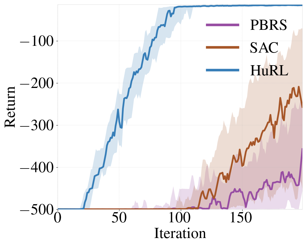
(a) Sparse-Reacher-v2

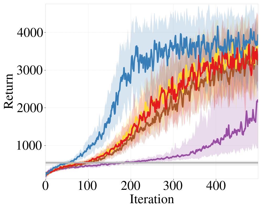
(b) Humanoid-v2

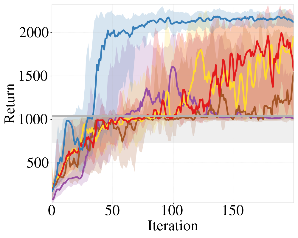
(c) Hopper-v2

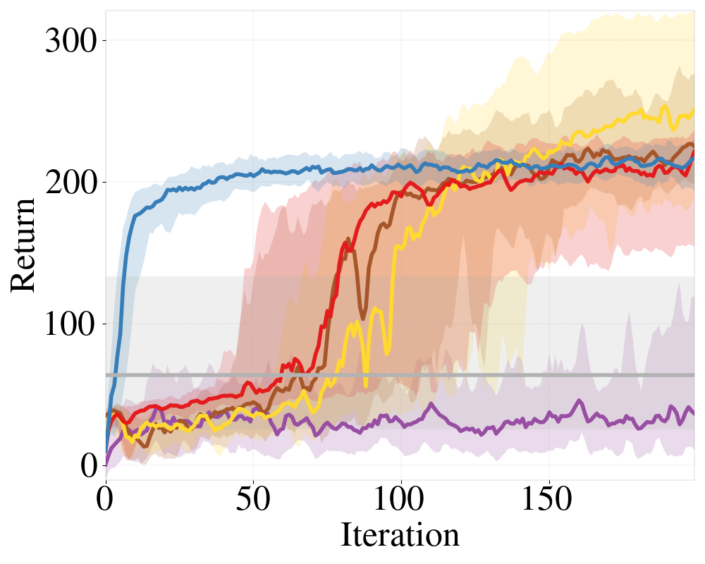
(d) Swimmer-v2

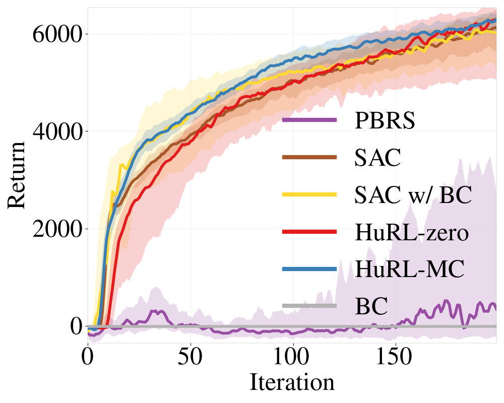
(e) HalfCheetah-v2

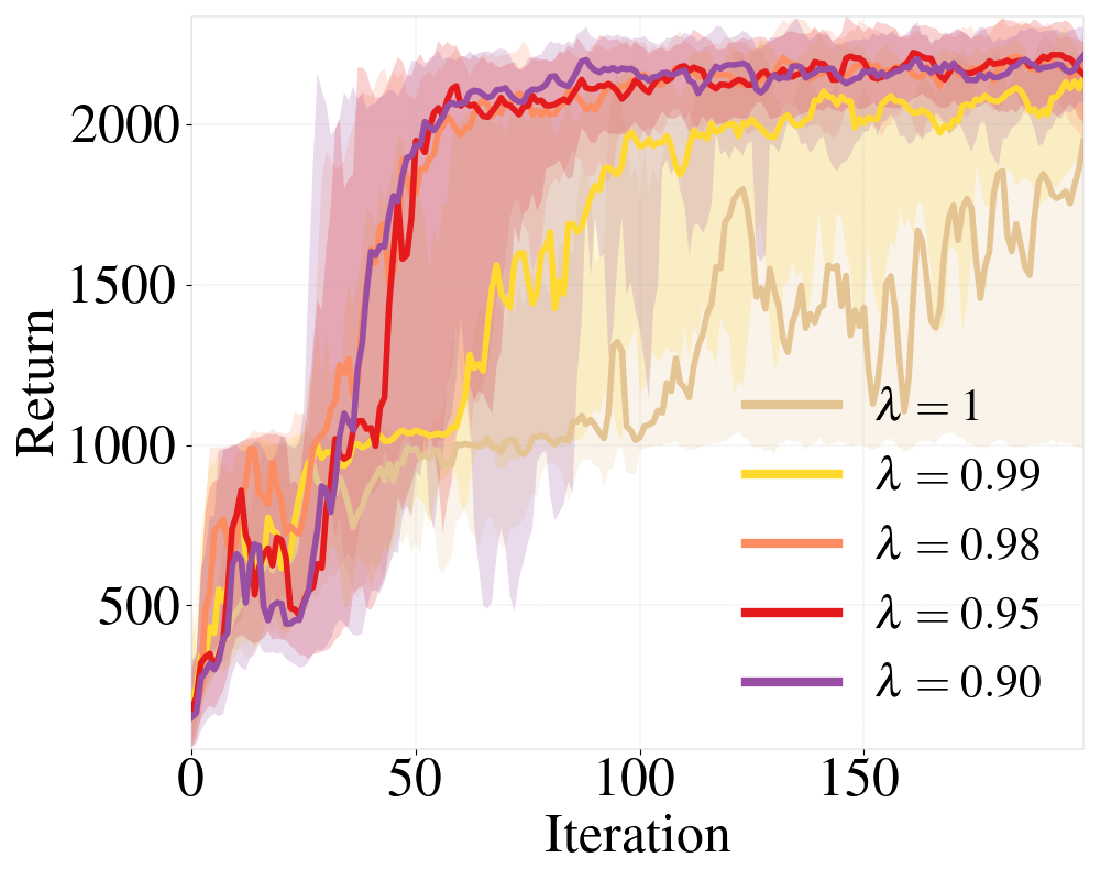
(f) $\lambda_{0}$ ablation.

Figure 2: Experimental results. (a) uses an engineered heuristic for a sparse reward problem; (b)-(e) use heuristics learned from offline data and share the same legend; (e) shows ablation results of different initial $\lambda_{0}$ in Hopper-v2. The plots show the $25$th, $50$th, $75$th percentiles of algorithm performance over 30 random seeds.

5.2 Results Summary

Fig. 2 shows the results on the MuJoCo environments. Overall, we see that HuRL is able to leverage engineered and learned heuristics to significantly improve the learning efficiency. This trend is consistent across all environments that we tested on.

For the sparse-reward experiments, we see that SAC and PBRS struggle to learn, while HuRL is able to converge to the optimal performance much faster. For the dense reward experiments, similarly HuRL-MC converges much faster, though the gain in HalfCheetah-v2 is minor and it might have converged to a worse local maximum in Swimmer-v2. In addition, we see that warm-starting SAC using BC (i.e. SAC w/ BC) can improve the learning efficiency compared with the vanilla SAC, but using BC alone does not result in a good policy. Lastly, we see that using the zero heuristic (HuRL-zero) with extra $\lambda$-scheduling does not further improve the performance of SAC w/ BC. This comparison verifies that the learned Monte-Carlo heuristic provides non-trivial information.

Interestingly, we see that applying PBRS to SAC leads to even worse performance than running SAC with the original reward. There are two reasons why SAC+PBRS is less desirable than SAC+HuRL as we discussed before: 1) PBRS changes the reward/value scales in the induced MDP, and popular RL algorithms like SAC are very sensitive to such changes. In contrast, HuRL induces values on the same scale as we show in Proposition 4.2. 2) In HuRL, we are effectively providing the algorithm some more side-information to let SAC shorten the horizon when the heuristic is good.

The results in Fig. 2 also have another notable aspect. Because the datasets used in the dense reward experiments contain trajectories collected by a range of policies, it is likely that BC suffers from disagreement in action selection among different policies. Nonetheless, training a heuristic using a basic Monte-Carlo regression seems to be less sensitive to these conflicts and still results in a helpful heuristic for HuRL. One explanation can be that heuristics are only functions of states, not of states and actions, and therefore the conflicts are minor. Another plausible explanation is that HuRL only uses the heuristic to guide learning, and does not completely rely on it to make decisions Thus, HuRL can be more robust to the heuristic quality, or, equivalently, to the quality of prior knowledge.

5.3 Ablation: Effects of Horizon Shortening

To further verify that the acceleration in Fig. 2 is indeed due to horizon shortening, we conducted an ablation study for HuRL-MC on Hopper-v2, whose results are presented in Fig. 2(f). HuRL-MC’s best $\lambda$-schedule hyperparameters on Hopper-v2, which are reflected in its performance in the aforementioned Fig. 2(c), induced a near-constant schedule at $\lambda=0.95$; to obtain the curves in Fig. 2(f), we ran HuRL-MC with constant-$\lambda$ schedules for several more $\lambda$ values. Fig. 2(f) shows that increasing $\lambda$ above $0.98$ leads to a performance drop. Since using a large $\lambda$ decreases bias and makes the reshaped MDP more similar to the original MDP, we conclude that the increased learning speed on Hopper-v2 is due to HuRL’s horizon shortening (coupled with the guidance provided by its heuristic).

6 Related Work

Discount regularization.

The horizon-truncation idea can be traced back to Blackwell optimality in the known MDP setting [18]. Reducing the discount factor amounts to running HuRL with a zero heuristic. Petrik and Scherrer [19], Jiang et al. [20, 21] study the MDP setting; Chen et al. [22] study POMDPs. Amit et al. [23] focus on discount regularization for Temporal Difference (TD) methods, while Van Seijen et al. [6] use a logarithmic mapping to lower the discount for online RL.

Reward shaping.

Reward shaping has a long history in RL, from the seminal PBRS work [29] to recent bilevel-optimization approaches [38]. Tessler and Mannor [5] consider a complementary problem to HuRL: given a discount $\gamma^{\prime}$, they find a reward $r^{\prime}$ that preserves trajectory ordering in the original MDP. Meanwhile there is a vast literature on bias-variance trade-off for online RL with horizon truncation. TD($\lambda$) [39, 40] and Generalized Advantage Estimates [41] blend value estimates across discount factors, while Sherstan et al. [42] use the discount factor as an input to the value function estimator. TD($\Delta$) [43] computes differences between value functions across discount factors.

Heuristics in model-based methods.

Classic uses of heuristics include A* [24], Monte-Carlo Tree Search (MCTS) [25], and Model Predictive Control (MPC) [44]. Zhong et al. [26] shorten the horizon in MPC using a value function approximator. Hoeller et al. [27] additionally use an estimate for the running cost to trade off solution quality and amount of computation. Bejjani et al. [28] show heuristic-accelerated truncated-horizon MPC on actual robots and tune the value function throughout learning. Bhardwaj et al. [7] augment MPC with a terminal value heuristic, which can be viewed as an instance of HuRL where the base algorithm is MPC. Asai and Muise [45] learn an MDP expressible in the STRIPS formalism that can benefit from relaxation-based planning heuristics. But HuRL is more general, as it does not assume model knowledge and can work in unknown environments.

Pessimistic extrapolation.

Offline RL techniques employ pessimistic extrapolation for robustness [30], and their learned value functions can be used as heuristics in HuRL. Kumar et al. [46] penalize out-of-distribution actions in off-policy optimization while Liu et al. [31] additionally use a variational auto-encoder (VAE) to detect out-of-distribution states. We experimented with VAE-filtered pessimistic heuristics in Appendix C. Even pessimistic offline evaluation techniques [16] can be useful in HuRL, since function approximation often induces extrapolation errors [47].

Heuristic pessimism vs. admissibility.

Our concept of heuristic pessimism can be easily confused for the well-established notion of admissibility [48], but in fact they are opposites. Namely, an admissible heuristic never underestimates $V^{*}$ (in the return-maximization setting), while a pessimistic one never overestimates $V^{*}$. Similarly, our notion of improvability is distinct from consistency: they express related ideas, but with regards to pessimistic and admissible value functions, respectively. Thus, counter-intuitively from the planning perspective, our work shows that for policy learning, inadmissible heuristics are desirable. Pearl [49] is one of the few works that has analyzed desirable implications of heuristic inadmissibility in planning.

Other warm-starting techniques.

HuRL is a new way to warm-start online RL methods. Bianchi et al. [50] use a heuristic policy to initialize agents’ policies. Hester et al. [10], Vinyals et al. [2] train a value function and policy using batch IL and then used them as regularization in online RL. Nair et al. [9] use off-policy RL on batch data and fine-tune the learned policy. Recent approaches of hybrid IL-RL have strong connections to HuRL [51, 17, 52]. In particular, Cheng et al. [17] is a special case of HuRL with a max-aggregation heuristic. Farahmand et al. [8] use several related tasks to learn a task-dependent heuristic and perform shorter-horizon planning or RL. Knowledge distillation approaches [53] can also be used to warm-start learning, but in contrast to them, HuRL expects prior knowledge in the form of state value estimates, not features, and doesn’t attempt to make the agent internalize this knowledge. A HuRL agent learns from its own environment interactions, using prior knowledge only as guidance. Reverse Curriculum approaches [54] create short horizon RL problems by initializing the agent close to the goal, and moving it further away as the agent improves. This gradual increase in the horizon inspires the HuRL approach. However, HuRL does not require the agent to be initialized on expert states and can work with many different base RL algorithms.

7 Discussion and Limitations

This work is an early step towards theoretically understanding the role and potential of heuristics in guiding RL algorithms. We propose a framework, HuRL, that can accelerate RL when an informative heuristic is provided. HuRL induces a horizon-based regularization of RL, complementary to existing warm-starting schemes, and we provide theoretical and empirical analyses to support its effectiveness. While this is a conceptual work without foreseeable societal impacts yet, we hope that it will help counter some of AI’s risks by making RL more predictable via incorporating prior into learning.

We remark nonetheless that the effectiveness of HuRL depends on the available heuristic. While HuRL can eventually solve the original RL problem even with a non-ideal heuristic, using a bad heuristic can slow down learning. Therefore, an important future research direction is to adaptively tune the mixing coefficient based on the heuristic quality with curriculum or meta-learning techniques. In addition, while our theoretical analysis points out a strong connection between good heuristics for HuRL and pessimistic offline RL, techniques for the latter are not yet scalable and robust enough for high-dimensional problems. Further research on offline RL can unlock the full potential of HuRL.

Checklist

1. For all authors…

   1. Do the main claims made in the abstract and introduction accurately reflect the paper’s contributions and scope? [Yes]

   2. Did you describe the limitations of your work? [Yes] Section 7.

   3. Did you discuss any potential negative societal impacts of your work? [Yes] Section 7. It is a conceptual work that doesn’t have foreseeable societal impacts yet.

   4. Have you read the ethics review guidelines and ensured that your paper conforms to them? [Yes]

2. If you are including theoretical results…

   1. Did you state the full set of assumptions of all theoretical results? [Yes] The assumptions are in the theorem, proposition, and lemma statements throughout the paper.

   2. Did you include complete proofs of all theoretical results? [Yes] Appendix A and Appendix B.

3. If you ran experiments…

   1. Did you include the code, data, and instructions needed to reproduce the main experimental results (either in the supplemental material or as a URL)? [Yes] In the supplemental material.

   2. Did you specify all the training details (e.g., data splits, hyperparameters, how they were chosen)? [Yes] Appendix C.

   3. Did you report error bars (e.g., with respect to the random seed after running experiments multiple times)? [Yes] Section 5 and Appendix C.

   4. Did you include the total amount of compute and the type of resources used (e.g., type of GPUs, internal cluster, or cloud provider)? [Yes] Appendix C.

4. If you are using existing assets (e.g., code, data, models) or curating/releasing new assets…

   1. If your work uses existing assets, did you cite the creators? [Yes] References [37], [32], and [33] in Section 5.1.

   2. Did you mention the license of the assets? [Yes] In Section 5.1.

   3. Did you include any new assets either in the supplemental material or as a URL? [Yes] Heuristic computation and scripts to run training.

   4. Did you discuss whether and how consent was obtained from people whose data you’re using/curating? [N/A]

   5. Did you discuss whether the data you are using/curating contains personally identifiable information or offensive content? [N/A]

5. If you used crowdsourcing or conducted research with human subjects…

   1. Did you include the full text of instructions given to participants and screenshots, if applicable? [N/A]

   2. Did you describe any potential participant risks, with links to Institutional Review Board (IRB) approvals, if applicable? [N/A]

   3. Did you include the estimated hourly wage paid to participants and the total amount spent on participant compensation? [N/A]

Appendix A Missing Proofs

We provide the complete proofs of the theorems stated in the main paper. We defer the proofs of the technical results to Appendix B.

A.1 Proof of Theorem 4.1

See 4.1

First we prove the equality using a new performance difference lemma that we will prove in Appendix B. This result may be of independent interest.

Lemma A.1 (General Performance Difference Lemma).

Consider the reshaped MDP $\widetilde{\mathcal{M}}$ defined by some $f:\SS\to\mathbb{R}$ and $\lambda\in[0,1]$. For any policy $\pi$, any state distribution $d_{0}$ and any $V:\SS\to\mathbb{R}$, it holds that

$$V(d_{0})-V^{\pi}(d_{0}) =\frac{\gamma(1-\lambda)}{1-\gamma}\mathbb{E}_{s,a\sim d^{\pi}}\mathbb{E}_{s^{\prime}|s,a}\left[h(s^{\prime})-V(s^{\prime})\right]$$

$$\quad+\lambda\left(V(d_{0})-\widetilde{V}^{\pi}(d_{0})\right)+\frac{1-\lambda}{1-\gamma}\left(V(d^{\pi})-\widetilde{V}^{\pi}(d^{\pi})\right)$$

Now take $V$ as $\widetilde{V}^{*}$ in the equality above. Then we can write

$$V^{*}(d_{0})-V^{\pi}(d_{0}) =\left(V^{*}(d_{0})-\widetilde{V}^{*}(d_{0})\right)+\frac{\gamma(1-\lambda)}{1-\gamma}\mathbb{E}_{s,a\sim d^{\pi}}\mathbb{E}_{s^{\prime}|s,a}\left[h(s^{\prime})-\widetilde{V}^{*}(s^{\prime})\right]$$

$$\quad+\lambda\left(\widetilde{V}^{*}(d_{0})-\widetilde{V}^{\pi}(d_{0})\right)+\frac{1-\lambda}{1-\gamma}\left(\widetilde{V}^{*}(d^{\pi})-\widetilde{V}^{\pi}(d^{\pi})\right)$$

which is the regret-bias decomposition.

Next we prove that these two terms are independent of constant offsets. For the regret term, this is obvious because shifting the heuristic by a constant would merely shift the reward by a constant. For the bias term, we prove the invariance below.

Proposition A.1.

$\mathrm{Bias}(h,\lambda,\pi)=\mathrm{Bias}(h+b,\lambda,\pi)$ for any $b\in\mathbb{R}$.

Proof.

Notice that any $b\in\mathbb{R}$ and $\pi$, $\widetilde{V}^{\pi}(s;f+b)-\widetilde{V}^{\pi}(s;f)=\sum_{t=0}^{\infty}(\lambda\gamma)^{t}(1-\lambda)\gamma b=\frac{(1-\lambda)\gamma}{1-\lambda\gamma}b$. Therefore, we can derive

$$\mathrm{Bias}(h+b,\lambda,\pi)-\mathrm{Bias}(h,\lambda,\pi) =-\frac{(1-\lambda)\gamma}{1-\gamma\lambda}b+\frac{\gamma(1-\lambda)}{1-\gamma}\mathbb{E}_{s,a\sim d^{\pi}}\mathbb{E}_{s^{\prime}|s,a}\left[b-\frac{(1-\lambda)\gamma}{1-\gamma\lambda}b\right]$$

$$=\frac{\gamma(1-\lambda)}{1-\gamma}b-\left(1+\frac{\gamma(1-\lambda)}{1-\gamma}\right)\frac{(1-\lambda)\gamma}{1-\gamma\lambda}b$$

Since

$$\left(1+\frac{\gamma(1-\lambda)}{1-\gamma}\right)\frac{(1-\lambda)\gamma}{1-\gamma\lambda}b=\frac{1-\gamma+\gamma(1-\lambda)}{1-\gamma}\frac{(1-\lambda)\gamma}{1-\gamma\lambda}b=\frac{1-\gamma\lambda}{1-\gamma}\frac{(1-\lambda)\gamma}{1-\gamma\lambda}b=\frac{(1-\lambda)\gamma}{1-\gamma}b$$

we have $\mathrm{Bias}(h+b,\lambda,\pi)-\mathrm{Bias}(h,\lambda,\pi)=0$. ∎

A.2 Proof of Proposition 4.1

See 4.1

Define the Bellman backup for the reshaped MDP:

$$(\widetilde{\mathcal{B}}V)(s,a)\coloneqq\widetilde{r}(s,a)+\widetilde{\gamma}\mathbb{E}_{s^{\prime}|s,a}[V(s^{\prime})]$$

Then by Lemma B.6 in Appendix B, we can rewrite the regret as

$$\lambda\left(\widetilde{V}^{*}(d_{0})-\widetilde{V}^{\pi}(d_{0})\right)+\frac{1-\lambda}{1-\gamma}\left(\widetilde{V}^{*}(d^{\pi})-\widetilde{V}^{\pi}(d^{\pi})\right)=\mathbb{E}_{\rho^{\pi}(d_{0})}\left[\sum_{t=0}^{\infty}\gamma^{t}\left(\widetilde{V}^{*}(s_{t})-(\widetilde{\mathcal{B}}\widetilde{V}^{*})(s_{t},a_{t})\right)\right]$$

Notice the equivalence $\widetilde{V}^{*}(s)-(\widetilde{\mathcal{B}}\widetilde{V}^{*})(s,a)=-\widetilde{A}^{*}(s,a)$. This concludes the proof.

A.3 Proof of Proposition 4.2

See 4.2

For the first statement, notice $\widetilde{r}(s,a)\in[0,1+\frac{(1-\lambda)\gamma}{1-\gamma}]$. Therefore, we have $\widetilde{V}^{\pi}(s)\geq 0$ as well as

$$\widetilde{V}^{\pi}(s) \leq\frac{1}{1-\lambda\gamma}\left(1+\frac{(1-\lambda)\gamma}{1-\gamma}\right)$$

$$=\frac{1}{1-\lambda\gamma}\frac{1-\gamma+(1-\lambda)\gamma}{1-\gamma}=\frac{1}{1-\gamma}$$

For the second statement, we just need to show the reshaped reward $\widetilde{r}(s,a)$ is linear in $\phi(s,a)$. This is straightforward because $\mathbb{E}_{s^{\prime}|s,a}[h(s^{\prime})]$ is linear in $\phi(s,a)$.

A.4 Proof of Corollary 4.1

See 4.1

By Theorem 4.1, we know that $\mathrm{Bias}(h,\lambda,\pi)=\mathrm{Bias}(h+b,\lambda,\pi)$ for any $b\in\mathbb{R}$. Now consider $b^{*}\in\mathbb{R}$ such that $\|h+b^{*}-V^{*}\|_{\infty}\leq\epsilon$. Then by Lemma B.5, we have also $\|h+b^{*}-\widetilde{V}^{\pi^{*}}\|_{\infty}\leq\epsilon+\frac{(1-\lambda)\gamma\epsilon}{1-\lambda\gamma}$.

Therefore, by Proposition 4.3, we can derive with definition of the bias,

$$\mathrm{Bias}(h,\lambda,\pi) =\mathrm{Bias}(h+b^{*},\lambda,\pi)$$

$$\leq(1-\lambda)\gamma\left(\mathcal{C}(\pi^{*},V^{*}-h-b^{*},\lambda\gamma)+\mathcal{C}(\pi,h+b^{*}-\widetilde{V}^{*},\gamma)\right)$$

$$\leq(1-\lambda)\gamma\left(\mathcal{C}(\pi^{*},V^{*}-h-b^{*},\lambda\gamma)+\mathcal{C}(\pi,h+b^{*}-\widetilde{V}^{\pi^{*}},\gamma)\right)$$

$$\leq(1-\lambda)\gamma\left(\frac{\epsilon}{1-\lambda\gamma}+\frac{1}{1-\gamma}(\epsilon+\frac{(1-\lambda)\gamma\epsilon}{1-\lambda\gamma})\right)$$

$$\leq(1-\lambda)\gamma\left(\frac{\epsilon}{1-\gamma}+\frac{1}{1-\gamma}(\epsilon+\frac{(1-\lambda)\gamma\epsilon}{1-\gamma})\right)$$

$$=\frac{2(1-\lambda)\gamma\epsilon}{1-\gamma}+\frac{(1-\lambda)^{2}\gamma^{2}\epsilon}{(1-\gamma)^{2}}\leq\frac{(1-\lambda\gamma)^{2}}{(1-\gamma)^{2}}\epsilon$$

A.5 Proof of Proposition 4.3

See 4.3 Recall the definition of bias:

$$\mathrm{Bias}(h,\lambda,\pi)=\left(V^{*}(d_{0})-\widetilde{V}^{*}(d_{0})\right)+\frac{\gamma(1-\lambda)}{1-\gamma}\mathbb{E}_{s,a\sim d^{\pi}}\mathbb{E}_{s^{\prime}|s,a}\left[h(s^{\prime})-\widetilde{V}^{*}(s^{\prime})\right]$$

For the first term, we can derive by performance difference lemma (Lemma B.1) and Lemma B.4

$$V^{*}(d_{0})-\widetilde{V}^{*}(d_{0}) \leq V^{*}(d_{0})-\widetilde{V}^{\pi^{*}}(d_{0})$$

$$=(1-\lambda)\gamma\mathbb{E}_{\rho^{\pi^{*}}(d_{0})}\left[\sum_{t=1}^{\infty}(\lambda\gamma)^{t-1}(V^{*}(s_{t})-h(s_{t}))\right]=(1-\lambda)\gamma\mathcal{C}(\pi,V^{*}-f,\lambda\gamma)$$

For the second term, we can rewrite it as

$$\frac{\gamma(1-\lambda)}{1-\gamma}\mathbb{E}_{s,a\sim d^{\pi}}\mathbb{E}_{s^{\prime}|s,a}\left[h(s^{\prime})-\widetilde{V}^{*}(s^{\prime})\right] =\gamma(1-\lambda)\mathbb{E}_{\rho^{\pi}(d_{0})}\left[\sum_{t=1}^{\infty}\gamma^{t-1}(h(s_{t})-\widetilde{V}^{*}(s_{t}))\right]$$

$$=(1-\lambda)\gamma\mathcal{C}(\pi^{*},f-\widetilde{V}^{*},\gamma)$$

A.6 Proof of Proposition 4.4

See 4.4

Let $d_{t}^{\pi}(s;s_{0})$ denote the state distribution at the $t$th step after running $\pi$ starting from $s_{0}\in\SS$ in $\mathcal{M}$ (i.e. $d_{0}^{\pi}(s;s_{0})={\mathbbm{1}}\{s=s_{0}\}$). Define the mixture

$$\widetilde{d}_{s_{0}}^{\pi}(s)\coloneqq(1-\widetilde{\gamma})\sum_{t=0}^{\infty}\widetilde{\gamma}^{t}d_{t}^{\pi}(s;s_{0})$$ (5)

where we recall the new discount $\widetilde{\gamma}=\gamma\lambda$ By performance difference lemma (Lemma B.1), we can write for any policy $\pi$ and any $s_{0}\in\smash{}$

$$\widetilde{V}^{\pi}(s_{0})-h(s_{0})=\frac{1}{1-\lambda\gamma}\mathbb{E}_{\widetilde{d}_{s_{0}}^{\pi}}[(\widetilde{\mathcal{B}}h)(s,a)-h(s)]$$

Notice that

$$(\widetilde{\mathcal{B}}h)(s,a) =\widetilde{r}(s,a)+\widetilde{\gamma}\mathbb{E}_{s^{\prime}|s,a}[h(s^{\prime})]$$

$$=r(s,a)+(1-\lambda)\gamma\mathbb{E}_{s^{\prime}|s,a}[h(s^{\prime})]+\lambda\gamma\mathbb{E}_{s^{\prime}|s,a}[h(s^{\prime})]$$

$$=r(s,a)+\gamma\mathbb{E}_{s^{\prime}|s,a}[h(s^{\prime})]=(\mathcal{B}h)(s,a)$$

Let $\pi$ denote the greedy policy of $\operatorname*{arg\,max}_{a}(\mathcal{B}h)(s,a)$. Then we have, by the improvability assumption we have $(\mathcal{B}h)(s,\pi)-h(s)\geq 0$ and therefore,

$$\widetilde{V}^{*}(s_{0})\geq\widetilde{V}^{\pi}(s_{0}) =h(s_{0})+\frac{1}{1-\lambda\gamma}\mathbb{E}_{\widetilde{d}_{s_{0}}^{\pi}}[(\widetilde{\mathcal{B}}h)(s,a)-h(s)]$$

$$=h(s_{0})+\frac{1}{1-\lambda\gamma}\mathbb{E}_{\widetilde{d}_{s_{0}}^{\pi}}[(\mathcal{B}h)(s,a)-h(s)]$$

$$\geq h(s_{0})$$

Since $s_{0}$ is arbitrary above, we have the desired statement.

A.7 Proof of Proposition 4.5

See 4.5

The proof is straightforward: We have $\max_{a}(\mathcal{B}h)(s,a)\geq(\mathcal{B}h)(s,\pi)\geq Q(s,\pi)=h(s)$, which is the definition of $h$ being improvable. For the argument of uniform lower bound, we chain the assumption $Q(s,a)\leq(\mathcal{B}h)(s,a)$:

$$h(s)=Q(s,\pi^{\prime}) =r(s,\pi^{\prime})+\gamma\mathbb{E}_{s^{\prime}|s,\pi^{\prime}}[h(s^{\prime})]$$

$$\leq r(s,\pi^{\prime})+\gamma\left(r(s^{\prime},\pi^{\prime}),+\gamma\mathbb{E}_{s^{\prime\prime}|s^{\prime},\pi^{\prime}}[h(s^{\prime\prime})]\right)$$

$$\leq V^{\pi^{\prime}}(s)$$

Appendix B Technical Lemmas

B.1 Lemmas of Performance Difference

Here we prove a general performance difference for the $\lambda$-weighting used in the reshaped MDPs. See A.1 Our new lemma includes the two below performance difference lemmas in the literature as special cases. Lemma B.2 can be obtained by setting $V=f$; Lemma B.1 can be obtained by further setting $\lambda=0$ (that is, Lemma B.1 is a special case of Lemma B.2 with $\lambda=0$; and Lemma A.1 generalizes both). The proofs of these existing performance difference lemmas do not depend on the new generalization in Lemma A.1, please refer to [55, 17] for details.

Lemma B.1 (Performance Difference Lemma [55, 17] ).

For any policy $\pi$, any state distribution $d_{0}$ and any $V:S\to\mathbb{R}$, it holds that

$$V(d_{0})-V^{\pi}(d_{0})=\frac{1}{1-\gamma}\mathbb{E}_{d^{\pi}}[V(s)-(\mathcal{B}V)(s,a)]$$

Lemma B.2 ($\lambda$-weighted Performance Difference Lemma [17]).

For any policy $\pi$, $\lambda\in[0,1]$, and $f:\SS\to\mathbb{R}$, it holds that

$$f(d_{0})-V^{\pi}(d_{0}) =\lambda\left(f(d_{0})-\widetilde{V}^{\pi}(d_{0})\right)+\frac{1-\lambda}{1-\gamma}\left(f(d^{\pi})-\widetilde{V}^{\pi}(d^{\pi})\right)$$

B.1.1 Proof of Lemma A.1

First, we use the standard performance difference lemma (Lemma B.1) in the original MDP and Lemma B.3 for the first and the last steps below,

$$V(d_{0})-V^{\pi}(d_{0}) =\frac{1}{1-\gamma}\mathbb{E}_{d^{\pi}}\left[V(s)-(\mathcal{B}V)(s,a)\right]$$

$$=\frac{1}{1-\gamma}\mathbb{E}_{d^{\pi}}\left[(\widetilde{\mathcal{B}}V)(s,a)-(\mathcal{B}V)(s,a)\right]+\frac{1}{1-\gamma}\mathbb{E}_{d^{\pi}}\left[V(s)-(\widetilde{\mathcal{B}}V)(s,a)\right]$$

$$=\frac{\gamma(1-\lambda)}{1-\gamma}\mathbb{E}_{s,a\sim d^{\pi}}\mathbb{E}_{s^{\prime}|s,a}\left[h(s^{\prime})-V(s^{\prime})\right]+\frac{1}{1-\gamma}\mathbb{E}_{s,a\sim d^{\pi}}\left[V(s)-(\widetilde{\mathcal{B}}V)(s,a)\right]$$

Finally, substituting the equality in Lemma B.6 into the above equality concludes the proof.

B.2 Properties of reshaped MDP

The first lemma is the difference of Bellman backups.

Lemma B.3.

For any $V:\SS\to\mathbb{R}$,

$$(\mathcal{B}V)(s,a)-(\widetilde{\mathcal{B}}V)(s,a) =(1-\lambda)\gamma\mathbb{E}_{s^{\prime}|s,a}[V(s^{\prime})-h(s^{\prime})]$$

Proof.

The proof follows from the definition of the reshaped MDP:

$$(\mathcal{B}V)(s,a)-(\widetilde{\mathcal{B}}V)(s,a)$$

$$=r(s,a)+\gamma\mathbb{E}_{s^{\prime}|s,a}[V(s^{\prime})]-r(s,a)-(1-\lambda)\gamma\mathbb{E}_{s^{\prime}|s,a}[h(s^{\prime})]-\gamma\lambda\mathbb{E}_{s^{\prime}|s,a}[V(s^{\prime})]$$

$$=(1-\lambda)\gamma\mathbb{E}_{s^{\prime}|s,a}[V(s^{\prime})-h(s^{\prime})]$$

∎

This lemma characterizes, for a policy, the difference in returns.

Lemma B.4.

For any policy $\pi$ and $h:\SS\to\mathbb{R}$,

$$V^{\pi}(s)-\widetilde{V}^{\pi}(s) =(1-\lambda)\gamma\mathbb{E}_{\rho^{\pi}(s)}\left[\sum_{t=1}^{\infty}(\lambda\gamma)^{t-1}(V^{\pi}(s_{t})-h(s_{t}))\right]$$

Proof.

The proof is based on performance difference lemma (Lemma B.1) applied in the reshaped MDP and Lemma B.3. Recall the definition $\widetilde{d}_{s_{0}}^{\pi}(s)$ in (5) and define $\widetilde{d}_{s_{0}}^{\pi}(s,a)=\widetilde{d}_{s_{0}}^{\pi}(s)\pi(a|s)$. For any $s_{0}\in\SS$,

$$V^{\pi}(s_{0})-\widetilde{V}^{\pi}(s_{0}) =\frac{1}{1-\gamma\lambda}\mathbb{E}_{s,a\sim\widetilde{d}_{s_{0}}^{\pi}}[V^{\pi}(s)-\widetilde{\mathcal{B}}V^{\pi}(s,a)]$$

$$=\frac{1}{1-\gamma\lambda}\mathbb{E}_{s,a\sim\widetilde{d}_{s_{0}}^{\pi}}[(\mathcal{B}V^{\pi})(s,a)-(\widetilde{\mathcal{B}}V^{\pi})(s,a)]$$

$$=\frac{(1-\lambda)\gamma}{1-\gamma\lambda}\mathbb{E}_{s,a\sim\widetilde{d}_{s_{0}}^{\pi}}\mathbb{E}_{s^{\prime}|s,a}[V^{\pi}(s^{\prime})-h(s^{\prime})]$$

Finally, substituting the definition of $\widetilde{d}_{s_{0}}^{\pi}$ finishes the proof. ∎

A consequent lemma shows that $h$ and $\widetilde{V}^{\pi}$ are close, when $h$ and $V^{\pi}$ are.

Lemma B.5.

For a policy $\pi$, suppose $-\epsilon_{l}\leq h(s)-V^{\pi}(s)\leq\epsilon_{u}$. It holds

$$-\epsilon_{l}-\frac{(1-\lambda)\gamma\epsilon_{u}}{1-\lambda\gamma}\leq h(s)-\widetilde{V}^{\pi}(s)\leq\epsilon_{u}+\frac{(1-\lambda)\gamma\epsilon_{l}}{1-\lambda\gamma}$$

Proof.

We prove the upper bound by Lemma B.4; the lower bound can be shown by symmetry.

$$h(s)-\widetilde{V}^{\pi}(s) \leq\epsilon_{u}+V^{\pi}(s)-\widetilde{V}^{\pi}(s)$$

$$=\epsilon_{u}+(1-\lambda)\gamma\mathbb{E}_{\rho^{\pi}(s)}\left[\sum_{t=1}^{\infty}(\lambda\gamma)^{t-1}(V^{\pi}(s_{t})-h(s_{t}))\right]$$

$$\leq\epsilon_{u}+\frac{(1-\lambda)\gamma\epsilon_{l}}{1-\lambda\gamma}$$

∎

The next lemma relates online Bellman error to value gaps.

Lemma B.6.

For any $\pi$ and $V:\SS\to\mathbb{R}$,

$$\frac{1}{1-\gamma}\left(\mathbb{E}_{d^{\pi}}\left[V(s)-(\widetilde{\mathcal{B}}V)(s,a)\right]\right)=\lambda\left(V(d_{0})-\widetilde{V}^{\pi}(d_{0})\right)+\frac{1-\lambda}{1-\gamma}\left(V(d^{\pi})-\widetilde{V}^{\pi}(d^{\pi})\right)$$

Proof.

We use Lemma B.3 in the third step below.

$$\mathbb{E}_{d^{\pi}}\left[V(s)-(\widetilde{\mathcal{B}}V)(s,a)\right]$$

$$=\mathbb{E}_{d^{\pi}}\left[V(s)-(\widetilde{\mathcal{B}}\widetilde{V}^{\pi})(s,a)\right]+\mathbb{E}_{d^{\pi}}\left[\widetilde{\mathcal{B}}\widetilde{V}^{\pi}(s,a)-(\widetilde{\mathcal{B}}V)(s,a)\right]$$

$$=\mathbb{E}_{d^{\pi}}\left[V(s)-\widetilde{V}^{\pi}(s)\right]+\mathbb{E}_{d^{\pi}}\left[(\widetilde{\mathcal{B}}\widetilde{V}^{\pi})(s,a)-(\widetilde{\mathcal{B}}V)(s)\right]$$

$$=\mathbb{E}_{d^{\pi}}\left[V(s)-\widetilde{V}^{\pi}(s)\right]-\lambda\gamma\mathbb{E}_{s,a\sim d^{\pi}}\mathbb{E}_{s^{\prime}|s,a}\left[\widetilde{V}^{\pi}(s^{\prime})-V(s^{\prime})\right]$$

$$=(1-\gamma)\mathbb{E}_{\rho^{\pi}(d_{0})}\left[\sum_{t=0}^{\infty}\gamma^{t}(V(s_{t})-\widetilde{V}^{\pi}(s_{t}))-\lambda\gamma^{t+1}(\widetilde{V}^{\pi}(s_{t+1})-V(s_{t+1}))\right]$$

$$=(1-\gamma)\lambda(V(d_{0})-\widetilde{V}^{\pi}(d_{0}))+(1-\gamma)(1-\lambda)\mathbb{E}_{\rho_{\pi}(d_{0})}\left[\sum_{t=0}^{\infty}\gamma^{t}(V(s_{t})-\widetilde{V}^{\pi}(s_{t}))\right]$$

∎

Appendix C Experiments

C.1 Details of the MuJoCo Experiments

We consider four dense reward MuJoCo environments (Hopper-v2, HalfCheetah-v2, Humanoid-v2, and Swimmer-v2) and a sparse reward version of Reacher-v2.

In the sparse reward Reacher-v2, the agent receives a reward of $0$ at the goal state (defined as $\|g(s)-e(s)\|\leq 0.01$ and $-1$ elsewhere, where $g(s)$ and $e(s)$ denote the goal state and the robot’s end-effector positions, respectively. We designed a heuristic $h(s)=r(s,a)-100\|e(s)-g(s)\|$, as this is a goal reaching task. Here the policy is randomly initialized, as no prior batch data is available before interactions.

In the dense reward experiments, we suppose that a batch of data collected by multiple behavioral policies are available before learning, and a heuristic is constructed by an offline policy evaluation algorithm from the batch data; in the experiments, we generated these behavioral policies by running SAC from scratch and saved the intermediate policies generated in training. We designed this heuristic generation experiment to simulate the typical scenario where offline data collected by multiple policies of various qualities is available before learning. In this case, a common method for inferring what values a good policy could get is to inspect the realized accumulated rewards in the dataset. For simplicity, we use basic Monte Carlo regression to construct heuristics, where a least squares regression problem was used to fit a fully connected neural network to predict the empirical returns on the trajectories in the sampled batch of data.

Specifically, for each dense reward Mujoco experiment, we ran SAC for 200 iterations and logged the intermediate policies for every 4 iterations, resulting in a total of 50 behavior policies. In each random seed of the experiment, we performed the following: We used each behavior policy to collect trajectories of at most 10,000 transition tuples, which gave about 500,000 offline data points over these 50 policies. These data were used to construct the Monte-Carlo regression data, which was done by computing the accumulated discounted rewards along sampled trajectories. Then we generated the heuristic used in the experiment by fitting a fully connected NN with (256,256)-hidden layers using default ADAM with step size 0.001 and minibatch size 128 for 30 epochs over this randomly generated dataset of 50 behavior policies.

For the dense reward Mujoco experiments, we also use behavior cloning (BC) with $\ell_{2}$ loss to warm start RL agents based on the same batch dataset of 500,000 offline data points. The base RL algorithm here is SAC, which is based on the standard implementation of Garage (MIT License) [37]. The policy and the value networks are fully connected neural networks, independent of each other. The policy is Tanh-Gaussian and the value network has a linear head.

Algorithms.

We compare the performance of different algorithms below. 1) BC 2) SAC 3) SAC with BC warm start (SAC w/ BC) 4) HuRL with a zero heuristic and BC warm start (HuRL-zero) 5) HuRL with the Monte-Carlo heuristic and BC warm start (HuRL-MC). For the HuRL algorithms, the mixing coefficient $\lambda_{n}$ is scheduled as

$$\lambda_{n} =\lambda_{0}+(1-\lambda_{0})\tanh\left(\frac{n-1}{\alpha N-1}\times\arctan(0.99)\right)/0.99$$

$$\eqqcolon\lambda_{0}+(1-\lambda_{0})c_{\omega}\tanh(\omega(n-1))$$

for $n=1,\dots,N$, where $\lambda_{0}\in[0,1]$ is the initial $\lambda$ and $\alpha>0$ controls the increasing rate. This schedule ensures that $\lambda_{N}=1$ when $\alpha=1$. Increasing $\alpha$ from $1$ makes $\lambda_{n}$ converge to $1$ slower.

We chose these algorithms to illustrate the effect of each additional warm-start component (BC and heuristics) added on top of the base algorithm SAC. HuRL-zero is SAC w/ BC but with an extra $\lambda$ schedule described above that further lowers the discount, whereas SAC and SAC w/ BC keep a constant discount factor.

Evaluation and Hyperparameters.

In each iteration, the RL agent has a fixed sample budget for environment interactions, and its performance is measured in terms of the undiscounted accumulated rewards (estimated by 10 rollouts) of the deterministic mean policy extracted from SAC. The hyperparameters used in the algorithms above were selected as follows. The selection was done by uniformly random grid search over the range of hyperparameters in Table 1 to maximize the AUC of the training curve.

Polcy step size	[0.00025, 0.0005, 0.001, 0.002]
Value step size	[0.00025, 0.0005, 0.001, 0.002]
Target step size	[0.005, 0.01, 0.02, 0.04]
$\gamma$	[0.9, 0.99, 0.999]
$\lambda_{0}$	[0.90, 0.95, 0.98, 0.99]
$\alpha$	[$10^{-5}$, 1.0, $10^{5}$]

Table 1: HuRL’s hyperparameter value grid for the MuJoCo experiments.

First, the learning rates (policy step size, value step size, target step size) and the discount factor of the base RL algorithm, SAC, were tuned for each environment to maximize the performance. This tuned discount factor is used as the de facto discount factor $\gamma$ of the original MDP $\mathcal{M}$. Fixing the hyperparameters above, $\lambda_{0}$ and $\alpha$ for the $\lambda$ schedule of HuRL were tuned for each environment and each heuristic. The tuned hyperparameters and the environment specifications are given in Tables 2 and 3 below. (The other hyperparameters, in addition to the ones tuned above, were selected manually and fixed throughout all the experiments).

Environment	Sparse-Reacher-v2
Obs. Dim	11
Action Dim	2
Evaluation horizon	500
$\gamma$	0.9
Batch Size	10000
Policy NN Architecture	(64,64)
Value NN Architecture	(256,256)
Polcy step size	0.00025
Value step size	0.00025
Target step size	0.02
Minibatch Size	128
Num. of Grad. Step per Iter.	1024
HuRL $\lambda_{0}$	0.5
HuRL-MC $\alpha$	$10^{5}$

Table 2: Sparse reward MuJoCo experiment configuration details. All the values other than $\lambda$-scheduler’s (i.e. those used in SAC) are shared across different algorithms in the comparison. All the neural networks here fully connected and have $\tanh$ activation; the numbers of hidden nodes are documented above. Note that when $\alpha=10^{5}$, effectively $\lambda_{n}=\lambda_{0}$ in the training iterations; when $\alpha=10^{-5}$, $\lambda_{n}\approx 1$ throughout.

Environment	Hopper-v2	HalfCheetah-v2	Swimmer-v2	Humanoid-v2
Obs. Dim	11	17	8	376
Action Dim	3	6	2	17
Evaluation horizon	1000	1000	1000	1000
$\gamma$	0.999	0.99	0.999	0.99
Batch Size	4000	4000	4000	10000
Policy NN Architecture	(64,64)	(64,64)	(64,64)	(256,256)
Value NN Architecture	(256,256)	(256,256)	(256,256)	(256,256)
Polcy step size	0.00025	0.00025	0.0005	0.002
Value step size	0.0005	0.0005	0.0005	0.00025
Target step size	0.02	0.04	0.0100	0.02
Num. of Behavioral Policies	50	50	50	50
Minibatch Size	128	128	128	128
Num. of Grad. Step per Iter.	1024	1024	1024	1024
HuRL-MC $\lambda_{0}$	0.95	0.99	0.95	0.9
HuRL-MC $\alpha$	$10^{5}$	$10^{5}$	1.0	1.0
HuRL-zero $\lambda_{0}$	0.98	0.99	0.99	0.95
HuRL-zero $\alpha$	$10^{-5}$	$10^{5}$	1.0	$10^{-5}$

Table 3: Dense reward MuJoCo experiment configuration details. All the values other than $\lambda$-scheduler’s (i.e. those used in SAC) are shared across different algorithms in the comparison. All the neural networks here fully connected and have $\tanh$ activation; the numbers of hidden nodes are documented above. Note that when $\alpha=10^{5}$, effectively $\lambda_{n}=\lambda_{0}$ in the training iterations; when $\alpha=10^{-5}$, $\lambda_{n}\approx 1$ throughout.

Finally, after all these hyperparameters were decided, we conducted additional testing runs with 30 different random seeds and report their statistics here. The randomness include the data collection process of the behavioral policies, training the heuristics from batch data, BC, and online RL, but the behavioral policies are fixed.

While this procedure takes more compute (the computation resources are reported below; tuning the base SAC takes the most compute), it produces more reliable results without (luckily or unluckily) using some hand-specified hyperparameters or a particular way of aggregating scores when tuning hyperparameters across environments. Empirically, we also found using constant $\lambda$ around $0.95\sim 0.98$ leads to good performance, though it may not be the best environment-specific choice.

Resources.

Each run of the experiment was done using an Azure Standard_H8 machine (8 Intel Xeon E5 2667 CPUs; memory 56 GB; base frequency 3.2 GHz; all cores peak frequency 3.3 GHz; single core peak frequency 3.6 GHz). The Hopper-v2, HalfCheetah-v2, Swimmer-v2 experiments took about an hour per run. The Humanoid-v2 experiments took about 4 hours. No GPU was used.

Extra Experiments with VAE-based Heuristics.

We conduct additional experiments of HuRL using a VAE-filtered pessimistic heuristic. This heuristic is essentially the same as the Monte-Carlo regression-based heuristic we discussed, except that an extra VAE (variational auto-encoder) is used to classify states into known and unknown states in view of the batch dataset, and then the predicted values of unknown states are set to be the lowest empirical return seen in the dataset. In implementation, this is done by training a state VAE (with a latent dimension of 32) to model the states in the batch data, and then a new state classified as unknown if its VAE loss is higher than 99-th percentile of the VAE losses seen on the batch data. The implementation and hyperparameters are based on the code from Liu et al. [31]. We note, however, that this basic VAE-based heuristic does not satisfy the assumption of Proposition 4.5.

These results are shown in Fig. 3, where HuRL-VAEMC denotes HuRL using this VAE-based heuristic. Overall, we see that such a basic pessimistic estimate does not improve the performance from the pure Monte-Carlo version (HuRL-MC); while it does improve the results slightly in HalfCheetah-v2, it gets worse results in Humanoid-v2 and Swimmer-v2 compared with HuRL-MC. Nonetheless, HuRL-VAEMC is still better than the base SAC.

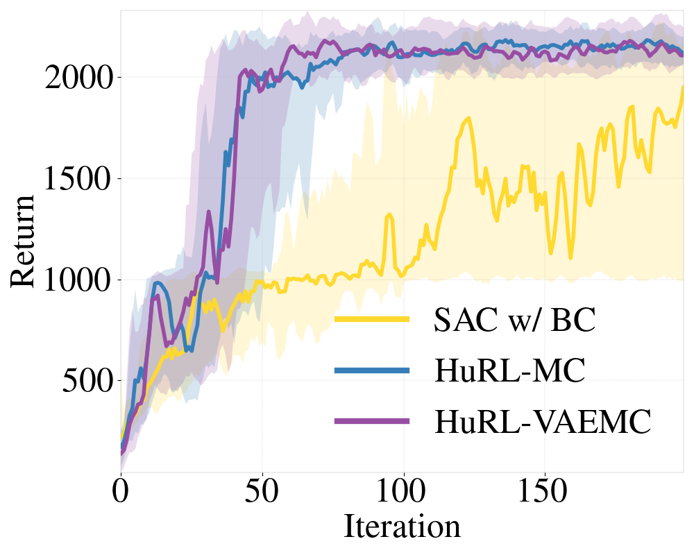
(a) Hopper-v2

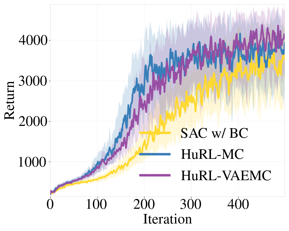
(b) Humanoid-v2

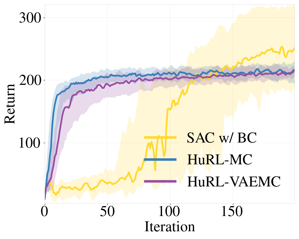
(c) Swimmer-v2

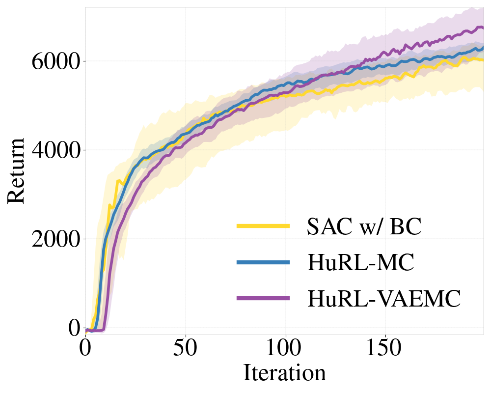
(d) HalfCheetah-v2

Figure 3: Extra experimental results of different MuJoCo environments. The plots show the $25$th, $50$th, $75$th percentiles of each algorithm’s performance over 30 random seeds.

C.2 Procgen Experiments

In addition to MuJoCo environments, where the agent has direct access to the true low-dimensional system state, we conducted experiments on the Procgen benchmark suite [56, 33]. The Procgen suite consists of 16 procedurally generated Atari-like game environments, whose main conceptual differences from MuJoCo environments are partial observability and much higher dimensionality of agents’ observations (RGB images). The 16 games are very distinct structurally, but each game has an unlimited number of levels that share common characteristics. All levels of a given game are situated in the same underlying state space and have the same transition function but differ in terms of the regions of the state space reachable within each level and in their observation spaces. We focus on the sample efficiency Procgen mode [33]: in each RL episode the agent faces a new game level, and is expected to eventually learn a single policy that performs well across all levels of the given game.

Besides the differences in environment characteristics between MuJoCo and Procgen, the Procgen experiments are also dissimilar in their design:

• In contrast to the MuJoCo experiments, where we assumed to be given a batch of data from which we constructed a heuristic and a warm-start policy, in the Procgen experiments we simulate a scenario where we are given only the heuristic function itself. Thus, we don’t warm-start the base algorithm with a BC policy when running HuRL.

• In the Procgen experiments, we share a single set of all hyperparameters’ values – those of the base algorithm, those of HuRL’s $\lambda$-scheduling, and those used for generating heuristics – across all 16 games. This is meant to simulate a scenario where HuRL is applied across a diverse set of problems using good but problem-independent hyperparameters.

Algorithms.

We used PPO [36] implemented in RLlib (Apache License 2.0) [57] as the base algorithm. We generated a heuristic for each game as follows:

• We ran PPO for $8M$ environment interaction steps and saved the policy after every $500K$ steps, for a total of 16 checkpoint policies.

• We ran the policies in a random order by executing 12000 environment interaction steps using each policy. For each rollout trajectory, we computed the discounted return for each observation in that trajectory, forming $\langle observation,return\rangle$ training pairs.

• We used this data to learn a heuristic via regression. We mixed the data, divided it into batches of 5000 training pairs and took a gradient step w.r.t. MSE computed over each batch. The learning rate was $10^{-4}$.

Our main algorithm, a HuRL flavor denoted as PPO-HuRL, is identical to the base PPO but uses the Monte-Carlo heuristic computed as above.

Hyperparameters and evaluation

The base PPO’s hyperparameters in RLlib were chosen to match PPO’s performance reported in the original Procgen paper [56] for the "easy" mode as closely as possible across all 16 games (Cobbe et al. [56] used a different PPO implementation with a different set of hyperparameters). As in that work, our agent used the IMPALA-CNN$\times 4$ network architecture [58, 56] without the LSTM. The heuristics employed the same architecture as well. We used a single set of hyperparameter values, listed in Table 4, for all Procgen games, both for policy learning and for generating the checkpoints for computing the heuristics.

Impala layer sizes	16, 32, 32
Rollout fragment length	256
Number of workers	0 (in RLlib, this means 1 rollout worker)
Number of environments per worker	64
Number of CPUs per worker	5
Number of GPUs per worker	0
Number of training GPUs	1
$\gamma$	0.99
SGD minibatch size	2048
Train batch size	4000
Number of SGD iterations	3
SGD learning rate	0.0005
Framestacking	off
Batch mode	truncate_episodes
Value function clip parameter	10.0
Value function loss coefficient	0.5
Value function share layers	true
KL coefficient	0.2
KL target	0.01
Entropy coefficient	0.01
Clip parameter	0.1
Gradient clip	null
Soft horizon	False
No done at end:	False
Normalize actions	False
Simple optimizer	False
Clip rewards	False
GAE $\lambda$	0.95
PPO-HuRL  $\lambda_{0}$	0.99
PPO-HuRL  $\alpha$	0.5

Table 4: Procgen experiment configuration details: RLlib PPO’s and HuRL’s hyperparameter values. All the values were shared across all 16 Procgen games.

$\lambda_{0}$	[0.95, 0.97, 0.985, 0.98, 0.99]
$\alpha$	[0.5, 0.75, 1.0, 3.0, 5.0]

Table 5: HuRL’s hyperparameter value grid for the Procgen experiments.

In order to choose values for PPO-HuRL’s hyperparameters $\alpha$ and $\lambda_{0}$, we fixed all of PPO’s hyperparameters, took the pre-computed heuristic for each game, and did a grid search over $\alpha$ and $\lambda_{0}$’s values listed in Table 5 to maximize the normalized average AUC across all games. To evaluate each hyperparameter value combination, we used 4 runs per game, each run using a random seed and lasting 8M environment interaction steps. The resulting values are listed in Table 4. Like PPO’s hyperparameters, they were kept fixed for all Procgen environments.

To obtain experimental results, we ran PPO and PPO-HuRL  with the aforementioned hyperparameters on each of 16 games 20 times, each run using a random seed and lasting 8M steps as in Mohanty et al. [33]. We report the 25th, 50th, and 75th-percentile training curves. Each of the reported training curves was computed by smoothing policy performance in terms of unnormalized game scores over the preceding 100 episodes.

Resources.

Each policy learning run used a single Azure ND6s machine (6 Intel Xeon E5-2690 v4 CPUs with 112 GB memory and base core frequency of 2.6 GHz; 1 P40 GPU with 24 GB memory). A single PPO run took approximately 1.5 hours on average. A single PPO-HuRL  run took approximately 1.75 hours.

Results.

The results are shown in Fig. 4. They indicate that, HuRL helps despite the highly challenging setup of this experiment: a) environments with a high-dimensional observation space; a) the chosen hyperparameter values being likely suboptimal for individual environments; c) the heuristics naively generated using Monte-Carlo samples from a mixture of policies of wildly varying quality; and d) the lack of policy warm-starting. We hypothesize that PPO-HuRL’s performance can be improved further with environment-specific hyperparameter tuning and a scheme for heuristic-quality-dependent adjustment of HuRL’s $\lambda$-schedules on the fly.

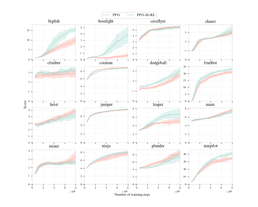
Figure 4: PPO-HuRL’s results on Procgen games. PPO-HuRL yields gains on half of the games and performs at par with PPO on most of the rest. Thus, on balance, PPO-HuRL helps despite the highly challenging setup of this experiment, but tuning HuRL’s $\lambda$-schedule on the fly depending on the quality of the heuristic can potentially make HuRL’s performance more robust in settings like this.

References

- Berner et al. [2019] Christopher Berner, Greg Brockman, Brooke Chan, Vicki Cheung, Przemysław Dębiak, Christy Dennison, David Farhi, Quirin Fischer, Shariq Hashme, Chris Hesse, et al. Dota 2 with large scale deep reinforcement learning. arXiv preprint arXiv:1912.06680, 2019.
- Vinyals et al. [2019] Oriol Vinyals, Igor Babuschkin, Wojciech M Czarnecki, Michaël Mathieu, Andrew Dudzik, Junyoung Chung, David H Choi, Richard Powell, Timo Ewalds, Petko Georgiev, et al. Grandmaster level in Starcraft II using multi-agent reinforcement learning. Nature, 575(7782):350–354, 2019.
- Dann and Brunskill [2015] Christoph Dann and Emma Brunskill. Sample complexity of episodic fixed-horizon reinforcement learning. In NIPS, 2015.
- Sidford et al. [2018] Aaron Sidford, Mengdi Wang, Xian Wu, Lin F Yang, and Yinyu Ye. Near-optimal time and sample complexities for solving Markov decision processes with a generative model. In NeurIPS, 2018.
- Tessler and Mannor [2020] Chen Tessler and Shie Mannor. Maximizing the total reward via reward tweaking. arXiv preprint arXiv:2002.03327, 2020.
- Van Seijen et al. [2019] Harm Van Seijen, Mehdi Fatemi, and Arash Tavakoli. Using a logarithmic mapping to enable lower discount factors in reinforcement learning. In NeurIPS, 2019.
- Bhardwaj et al. [2021] Mohak Bhardwaj, Sanjiban Choudhury, and Byron Boots. Blending mpc & value function approximation for efficient reinforcement learning. In ICLR, 2021.
- Farahmand et al. [2016] Amir-massoud Farahmand, Daniel N Nikovski, Yuji Igarashi, and Hiroki Konaka. Truncated approximate dynamic programming with task-dependent terminal value. In AAAI, 2016.
- Nair et al. [2020] Ashvin Nair, Murtaza Dalal, Abhishek Gupta, and Sergey Levine. Accelerating online reinforcement learning with offline datasets. arXiv preprint arXiv:2006.09359, 2020.
- Hester et al. [2018] Todd Hester, Matej Vecerik, Olivier Pietquin, Marc Lanctot, Tom Schaul, Bilal Piot, Dan Horgan, John Quan, Andrew Sendonaris, Ian Osband, et al. Deep Q-learning from demonstrations. In AAAI, 2018.
- Mausam and Kolobov [2012] Mausam and Andrey Kolobov. Planning with Markov decision processes: An AI perspective. Synthesis Lectures on Artificial Intelligence and Machine Learning, 6:1–210, 2012.
- Foster and Rakhlin [2020] Dylan Foster and Alexander Rakhlin. Beyond UCB: Optimal and efficient contextual bandits with regression oracles. In ICML, 2020.
- Hoffmann and Nebel [2001] J. Hoffmann and B. Nebel. The FF planning system: Fast plan generation through heuristic search. Journal of Artificial Intelligence Research, 14:253–302, 2001.
- Richter and Westphal [2010] S. Richter and M. Westphal. The LAMA planner: Guiding cost-based anytime planning with landmarks. Journal of Artificial Intelligence Research, 39:127–177, 2010.
- Kolobov et al. [2010] Andrey Kolobov, Mausam, and Daniel S. Weld. Classical planning in MDP heuristics: With a little help from generalization. In AAAI, 2010.
- Gulcehre et al. [2021] Caglar Gulcehre, Sergio Gómez Colmenarejo, Ziyu Wang, Jakub Sygnowski, Thomas Paine, Konrad Zolna, Yutian Chen, Matthew Hoffman, Razvan Pascanu, and Nando de Freitas. Regularized behavior value estimation. arXiv preprint arXiv:2103.09575, 2021.
- Cheng et al. [2020] Ching-An Cheng, Andrey Kolobov, and Alekh Agarwal. Policy improvement via imitation of multiple oracles. In NeurIPS, 2020.
- Blackwell [1962] David Blackwell. Discrete dynamic programming. The Annals of Mathematical Statistics, pages 719–726, 1962.
- Petrik and Scherrer [2008] Marek Petrik and Bruno Scherrer. Biasing approximate dynamic programming with a lower discount factor. In NIPS, 2008.
- Jiang et al. [2015] Nan Jiang, Alex Kulesza, Satinder Singh, and Richard Lewis. The dependence of effective planning horizon on model accuracy. In AAMAS, 2015.
- Jiang et al. [2016] Nan Jiang, Satinder Singh, and Ambuj Tewari. On structural properties of mdps that bound loss due to shallow planning. In IJCAI, 2016.
- Chen et al. [2018] Yi-Chun Chen, Mykel J Kochenderfer, and Matthijs TJ Spaan. Improving offline value-function approximations for pomdps by reducing discount factors. In IROS, 2018.
- Amit et al. [2020] Ron Amit, Ron Meir, and Kamil Ciosek. Discount factor as a regularizer in reinforcement learning. In ICML, 2020.
- Hart et al. [1968] Peter E Hart, Nils J Nilsson, and Bertram Raphael. A formal basis for the heuristic determination of minimum cost paths. IEEE Transactions on Systems Science and Cybernetics, 4(2):100–107, 1968.
- Browne et al. [2012] Cameron B Browne, Edward Powley, Daniel Whitehouse, Simon M Lucas, Peter I Cowling, Philipp Rohlfshagen, Stephen Tavener, Diego Perez, Spyridon Samothrakis, and Simon Colton. A survey of monte carlo tree search methods. IEEE Transactions on Computational Intelligence and AI in games, 4(1):1–43, 2012.
- Zhong et al. [2013] Mingyuan Zhong, Mikala Johnson, Yuval Tassa, Tom Erez, and Emanuel Todorov. Value function approximation and model predictive control. In IEEE International Symposium on Adaptive Dynamic Programming and Reinforcement Learning, pages 100–107, 2013.
- Hoeller et al. [2020] David Hoeller, Farbod Farshidian, and Marco Hutter. Deep value model predictive control. In CoRL, 2020.
- Bejjani et al. [2018] Wissam Bejjani, Rafael Papallas, Matteo Leonetti, and Mehmet R Dogar. Planning with a receding horizon for manipulation in clutter using a learned value function. In Humanoids, pages 1–9, 2018.
- Ng et al. [1999] Andrew Y Ng, Daishi Harada, and Stuart Russell. Policy invariance under reward transformations: Theory and application to reward shaping. In ICML, 1999.
- Jin et al. [2020] Ying Jin, Zhuoran Yang, and Zhaoran Wang. Is pessimism provably efficient for offline RL? arXiv preprint arXiv:2012.15085, 2020.
- Liu et al. [2020] Yao Liu, Adith Swaminathan, Alekh Agarwal, and Emma Brunskill. Provably good batch off-policy reinforcement learning without great exploration. In NeurIPS, 2020.
- Todorov et al. [2012] Emanuel Todorov, Tom Erez, and Yuval Tassa. Mujoco: A physics engine for model-based control. In IROS, 2012.
- Mohanty et al. [2021] Sharada Mohanty, Jyotish Poonganam, Adrien Gaidon, Andrey Kolobov, Blake Wulfe, Dipam Chakraborty, Gražvydas Šemetulskis, João Schapke, Jonas Kubilius, Jurgis Pašukonis, Linas Klimas, Matthew Hausknecht, Patrick MacAlpine, Quang Nhat Tran, Thomas Tumiel, Xiaocheng Tang, Xinwei Chen, Christopher Hesse, Jacob Hilton, William Hebgen Guss, Sahika Genc, John Schulman, and Karl Cobbe. Measuring sample efficiency and generalization in reinforcement learning benchmarks: NeurIPS 2020 Procgen benchmark. arXiv preprint arXiv:2103.15332, 2021.
- Jin et al. [2018] Chi Jin, Zeyuan Allen-Zhu, Sebastien Bubeck, and Michael I Jordan. Is Q-learning provably efficient? In NeurIPS, 2018.
- Haarnoja et al. [2018] Tuomas Haarnoja, Aurick Zhou, Pieter Abbeel, and Sergey Levine. Soft actor-critic: Off-policy maximum entropy deep reinforcement learning with a stochastic actor. In ICML, 2018.
- Schulman et al. [2017] John Schulman, Filip Wolski, Prafulla Dhariwal, Alec Radford, and Oleg Klimov. Proximal policy optimization algorithms. arXiv preprint arXiv:1707.06347, 2017.
- garage contributors [2019] The garage contributors. Garage: A toolkit for reproducible reinforcement learning research. https://github.com/rlworkgroup/garage, 2019.
- Hu et al. [2020] Yujing Hu, Weixun Wang, Hangtian Jia, Yixiang Wang, Yingfeng Chen, Jianye Hao, Feng Wu, and Changjie Fan. Learning to utilize shaping rewards: A new approach of reward shaping. In NeurIPS, 2020.
- Seijen and Sutton [2014] Harm Seijen and Rich Sutton. True online td (lambda). In ICML, 2014.
- Efroni et al. [2018] Yonathan Efroni, Gal Dalal, Bruno Scherrer, and Shie Mannor. Beyond the one-step greedy approach in reinforcement learning. In ICML, 2018.
- Schulman et al. [2016] John Schulman, Philipp Moritz, Sergey Levine, Michael Jordan, and Pieter Abbeel. High-dimensional continuous control using generalized advantage estimation. In ICLR, 2016.
- Sherstan et al. [2020] Craig Sherstan, Shibhansh Dohare, James MacGlashan, Johannes Günther, and Patrick M Pilarski. Gamma-nets: Generalizing value estimation over timescale. In AAAI, 2020.
- Romoff et al. [2019] Joshua Romoff, Peter Henderson, Ahmed Touati, Emma Brunskill, Joelle Pineau, and Yann Ollivier. Separating value functions across time-scales. In ICML, 2019.
- Richalet et al. [1978] Jacques Richalet, André Rault, JL Testud, and J Papon. Model predictive heuristic control. Automatica, 14(5):413–428, 1978.
- Asai and Muise [2020] Masataro Asai and Christian Muise. Learning neural-symbolic descriptive planning models via cube-space priors: The voyage home (to strips). In IJCAI, 2020.
- Kumar et al. [2020] Aviral Kumar, Aurick Zhou, George Tucker, and Sergey Levine. Conservative q-learning for offline reinforcement learning. In NeurIPS, 2020.
- Lu et al. [2018] Tyler Lu, Dale Schuurmans, and Craig Boutilier. Non-delusional q-learning and value iteration. In NeurIPS, 2018.
- Russell and Norvig [2020] Stuart J. Russell and Peter Norvig. Artificial Intelligence: A Modern Approach. Pearson, 4th edition, 2020.
- Pearl [1981] Judea Pearl. Heuristic search theory: Survey of recent results. In IJCAI, 1981.
- Bianchi et al. [2013] Reinaldo AC Bianchi, Murilo F Martins, Carlos HC Ribeiro, and Anna HR Costa. Heuristically-accelerated multiagent reinforcement learning. IEEE transactions on cybernetics, 44(2):252–265, 2013.
- Sun et al. [2017] Wen Sun, Arun Venkatraman, Geoffrey J Gordon, Byron Boots, and J Andrew Bagnell. Deeply aggrevated: Differentiable imitation learning for sequential prediction. In ICML, 2017.
- Sun et al. [2018] Wen Sun, J Andrew Bagnell, and Byron Boots. Truncated horizon policy search: Combining reinforcement learning & imitation learning. In ICLR, 2018.
- Hinton et al. [2015] Geoffrey Hinton, Oriol Vinyals, and Jeff Dean. Distilling the knowledge in a neural network. arXiv preprint arXiv:1503.02531, 2015.
- Florensa et al. [2017] Carlos Florensa, David Held, Markus Wulfmeier, Michael Zhang, and Pieter Abbeel. Reverse curriculum generation for reinforcement learning. In CoRL, 2017.
- Kakade and Langford [2002] Sham Kakade and John Langford. Approximately optimal approximate reinforcement learning. In ICML, 2002.
- Cobbe et al. [2020] Karl Cobbe, Christopher Hesse, Jacob Hilton, and John Schulman. Leveraging procedural generation to benchmark reinforcement learning. In ICML, 2020.
- Liang et al. [2018] Eric Liang, Richard Liaw, Robert Nishihara, Philipp Moritz, Roy Fox, Ken Goldberg, Joseph Gonzalez, Michael Jordan, and Ion Stoica. RLlib: Abstractions for distributed reinforcement learning. In ICML, 2018.
- Espeholt et al. [2018] Lasse Espeholt, Hubert Soyer, Remi Munos, Karen Simonyan, Vlad Mnih, Tom Ward, Yotam Doron, Vlad Firoiu, Tim Harley, Iain Dunning, Shane Legg, and Koray Kavukcuoglu. IMPALA: Scalable distributed deep-RL with importance weighted actor-learner architectures. In ICML, 2018.