Semiparametric inference on Gini indices of two semicontinuous populations under density ratio models

Meng Yuan,  Pengfei Li  and  Changbao Wu

 

The Gini index is a popular inequality measure with many applications in social and economic studies. This paper studies semiparametric inference on the Gini indices of two semicontinuous populations. We characterize the distribution of each semicontinuous population by a mixture of a discrete point mass at zero and a continuous skewed positive component. A semiparametric density ratio model is then employed to link the positive components of the two distributions. We propose the maximum empirical likelihood estimators of the two Gini indices and their difference, and further investigate the asymptotic properties of the proposed estimators. The asymptotic results enable us to construct confidence intervals and perform hypothesis tests for the two Gini indices and their difference. We show that the proposed estimators are more efficient than the existing fully nonparametric estimators. The proposed estimators and the asymptotic results are also applicable to cases without excessive zero values. Simulation studies show the superiority of our proposed method over existing methods. Two real-data applications are presented using the proposed methods.

Keywords: Density ratio model, zero-excessive data, empirical likelihood, equality test.

 

1 Introduction

The Gini index, first proposed by Gini (1912), has been widely used to measure population inequality. In economic studies, it is an important measure of income or wealth inequality among individuals or households in a particular population (Wang et al., 2016; Peng, 2011). In life expectancy studies, it is used to describe the concentration of survival times and to evaluate inequality among people in the target population (Bonetti et al., 2009; Lv et al., 2017). The index is closely related to the Lorenz curve (Lorenz, 1905), a widely used measure for the size distribution of income or wealth. It is the ratio of the area between the Lorenz curve and the 45-degree line to the area under the 45-degree line. Hence, the Gini index ranges from 0 to 1, with 0 indicating perfect equality and 1 for extreme inequality.

Study variables such as income and survival time are often modelled by using a positive continuous distribution. One important scenario in applications is that there are two related populations, each containing a sizeable zero values for the study variable. The inferential problems can be on the Gini index for each population separately or the difference of the two Gini indices. The scenario is quite common in practice but efficient inferential procedures are not available in the existing literature.

In this paper, we propose new semiparametric inference procedures for the Gini indices of two semicontinuous populations. Specifically, suppose that we have two independent samples from two related populations with values of the study variable $X$ generated from the following mixture models:

$$(X_{i1},\cdots,X_{in_{i}})\sim F_{i}(x)=\nu_{i}I(x\geq 0)+(1-\nu_{i})I(x>0)G_{i}(x),\leavevmode\nobreak\ \leavevmode\nobreak\ \leavevmode\nobreak\ \mbox{for\leavevmode\nobreak\ }\leavevmode\nobreak\ i=0,1,$$ (1)

where $\nu_{i}$ is the zero proportion in population $i$, $n_{i}$ is the sample size for sample $i$, $I(\cdot)$ is an indicator function, and $G_{i}(\cdot)$ is the cumulative distribution function (CDF) of the positive observations in sample $i$. For population $i=0,1$, the Gini index can be equivalently defined (David, 1968) as

$$\mathcal{G}_{i}=\frac{D_{i}}{2\mu_{i}},$$ (2)

where $D_{i}=E(|X_{i1}-X_{i2}|)$ is the expected absolute difference of $X$ for two randomly selected units from population $i$ and $\mu_{i}=E(X_{i1})$ is the expectation of population $i$. Our discussions in this paper focus on statistical inferences on $\mathcal{G}_{0}$, $\mathcal{G}_{1}$, and $\mathcal{G}_{0}-\mathcal{G}_{1}$. It is worth mentioning that although our results are presented for cases where the two populations contain excess zeros for the study variable, the proposed methods and the theoretical results are also applicable to cases without excess zeros, i.e., $\nu_{i}=0$ in model (1). In addition, inferences on a general function of $\mathcal{G}_{0}$ and $\mathcal{G}_{1}$ can also be conducted. See Section 2 for further discussion.

Samples with positive outcomes only, i.e., $\nu_{i}=0$ in model (1), are common in studies of family income or wealth or a country’s gross domestic products (Gastwirth, 1972; Cowell, 2011). For instance, all the household incomes are positive in the 1997 Family and Income and Expenditure Survey conducted by the Philippine Statistics Authority. More details can be found in Section 4. Samples with a mixture of excess zero values and skewed positive outcomes, i.e., $\nu_{i}>0$ in model (1), naturally arise in studies of expenditure data and health cost data (Zhou & Tu, 1999; Zhou & Tu, 2000; Zhou & Cheng, 2008). For example, Zhou & Cheng (2008) presented a dataset from the assessment of inpatient charges (see Section 4), and most patients with uncomplicated hypertension had no hospitalization and therefore zero costs. This paper systematically studies both cases ($\nu_{i}=0$ and $\nu_{i}>0$) in a unified framework via model (1).

Many studies of the Gini index have applied nonparametric methods. For example, point estimators of $\mathcal{G}_{0}$, $\mathcal{G}_{1}$, and $\mathcal{G}_{0}-\mathcal{G}_{1}$ and their asymptotic variance estimation have been discussed in Hoeffding (1948), Anand (1983), Ogwang (2000), Giles (2004), Modarres & Gastwirth (2006), Yitzhaki (1991), Karagiannis & Kovacevic (2000), and Davidson (2009). See Wang & Zhao (2016) for a detailed review. Qin et al. (2010) and Peng (2011) used the empirical likelihood (EL) method (Owen, 2001) to construct confidence intervals (CIs) for the index. More recently, Wang et al. (2016) derived the jackknife EL (JEL). Peng (2011) and Wang & Zhao (2016) compared two Gini indices of independent or correlated populations using the EL method and the JEL method, respectively.

Fully nonparametric methods are robust to potential model misspecifications on the $F_{i}$’s. However, these methods ignore the characteristics common to the two samples and/or the relation between the two populations, which have been shown to be useful for more efficient statistical inferences; see, for instance, the studies on the strengths of lumber produced in Canada in different years (Chen & Liu, 2013; Cai et al., 2017; Cai & Chen, 2018) and biomarkers for the diagnosis of disease in case and control groups (Yuan et al., 2020, 2021).

To combine the information from the two samples without making risky parametric distributional assumptions, we model the CDFs of the positive observations $G_{0}$ and $G_{1}$ in model (1) via a density ratio model (DRM) (Anderson, 1979; Qin, 2017). Let $dG_{i}$ be the probability density function of $G_{i}$, $i=0,1$. The DRM postulates that

$$dG_{1}(x)=\exp\{\alpha+\boldsymbol{\beta}^{\top}\boldsymbol{q}(x)\}dG_{0}(x)=\exp\{\boldsymbol{\theta}^{\top}\boldsymbol{Q}(x)\}dG_{0}(x)\,,$$ (3)

where $\boldsymbol{\theta}=(\alpha,\boldsymbol{\beta}^{\top})^{\top}$ is the vector of unknown parameters and $\boldsymbol{Q}(x)=(1,\boldsymbol{q}(x)^{\top})^{\top}$ with $\boldsymbol{q}(x)$ being a $d$-dimensional, prespecified, nontrivial basis function. Note that the baseline distribution $G_{0}$ is completely unspecified, which allows the DRM to embrace many distributions that are commonly used in the study of the Gini index (Moothathu, 1985, 1989, 1990). For example, when $\boldsymbol{q}(x)=\log(x)$, the DRM includes two log-normal distributions with the same variance with respect to the log-scale, two Pareto distributions with the same scale parameter, and two chi-square distributions with different degrees of freedom; when $\boldsymbol{q}(x)=x$, the DRM includes two exponential distributions with different rates. The DRM is closely related to the well-studied logistic regression (Qin & Zhang, 1997) and is broader than the Cox proportional hazard model (Jiang & Tu, 2012).

The DRM has served as a useful and flexible inferential platform for many statistical problems, including quantile and quantile-function estimation (Chen & Liu, 2013; Yuan et al., 2021; Chen et al., 2021), receiver operating characteristic analysis (Qin & Zhang, 2003; Chen et al., 2016; Yuan et al., 2021), hypothesis-testing problems (Fokianos et al., 2001; Cai et al., 2017), and data integration (Qin et al., 2015; Yuan et al., 2021). Recently, the DRM has been used for semicontinuous data. For example, Wang et al. (2017) and Wang et al. (2018) developed EL ratio (ELR) statistics for testing the homogeneity of distributions and the equality of population means, respectively. Yuan et al. (2020) proposed estimators of linear functionals of two semicontinuous populations. To the best of our knowledge, inferential procedures for two Gini indices $\mathcal{G}_{0}$, $\mathcal{G}_{1}$ and their difference $\mathcal{G}_{0}-\mathcal{G}_{1}$ have not been explored under the mixture model (1) and the DRM (3). This paper aims to fill this void.

Our contributions can be summarized as follows. We first propose the maximum EL estimators (MELEs) of $\mathcal{G}_{0}$, $\mathcal{G}_{1}$, and $\mathcal{G}_{0}-\mathcal{G}_{1}$ under models (1) and (3). Using techniques from U-statistics and V-statistics, we derive the asymptotic normality of the MELEs of $\mathcal{G}_{0}$, $\mathcal{G}_{1}$, and $\mathcal{G}_{0}-\mathcal{G}_{1}$ and show that their asymptotic variances are smaller than those of nonparametric estimators. These asymptotic results are used to construct Wald-type CIs for $\mathcal{G}_{0}$, $\mathcal{G}_{1}$, and $\mathcal{G}_{0}-\mathcal{G}_{1}$ and obtain a Wald-type statistic for testing $H_{0}:\mathcal{G}_{0}=\mathcal{G}_{1}$. The proposed methods and asymptotic results are applicable to both $\nu_{i}=0$ and $\nu_{i}>0$ in model (1). Extensive simulation studies and applications to two real datasets demonstrate the advantages of our proposed methods over existing ones. Software for implementing the proposed methods and Qin & Zhang (1997)’s goodness-of-fit test for the DRM assumption in (3) has been developed in R and is available from the authors upon request.

The rest of the paper is organized as follows. In Section 2, we propose the MELEs of $\mathcal{G}_{0}$, $\mathcal{G}_{1}$, and $\mathcal{G}_{0}-\mathcal{G}_{1}$ and study their asymptotic properties under the assumed semiparametric density ratio model. We construct CIs and conduct hypothesis tests on $\mathcal{G}_{0}$, $\mathcal{G}_{1}$, and $\mathcal{G}_{0}-\mathcal{G}_{1}$ based on the theoretical results. Results from simulation studies are presented in Section 3, and applications to two real-world datasets are given in Section 4. We conclude the paper with a discussion in Section 5. Proofs and technical details and additional simulation results are provided in the Supplementary Material.

2 Main Results

Let $n_{i0}$ and $n_{i1}$ be the (random) numbers of zero observations and positive observations, respectively, in each sample $i=0,1$. It follows that $n_{i}=n_{i0}+n_{i1}$ for $i=0,1$. Without loss of generality, we assume that the first $n_{i1}$ observations in group $i$, $X_{i1},\cdots,X_{in_{i1}}$, are positive, and the remaining $n_{i0}$ observations are 0. Let $n$ be the total (fixed) sample size, i.e., $n=n_{0}+n_{1}$.

2.1 The MELEs of $\mathcal{G}_{0}$ and $\mathcal{G}_{1}$

In this section, we develop the EL function and present the MELEs of $\mathcal{G}_{0}$ and $\mathcal{G}_{1}$. Based on the two samples from model (1), the full likelihood function is given by

$$L_{n} = \prod_{i=0}^{1}\left[\left\{v_{i}^{n_{i0}}\left(1-v_{i}\right)^{n_{i1}}\right\}\prod_{j=1}^{n_{i1}}dG_{i}\left(X_{ij}\right)\right],$$ (4)

which is the product of two likelihood components: one from the number of zero observations and the other from the positive observations.

Following the EL principle (Owen, 2001) and with the help of the DRM (3), we use the combined sample to model $G_{0}$ via

$$G_{0}(x)=\sum_{i=0}^{1}\sum_{j=1}^{n_{i1}}p_{ij}I(X_{ij}\leq x),$$ (5)

where $p_{ij}=dG_{0}(X_{ij})$ for $i=0,1$ and $j=1,\ldots,n_{i1}$. The model for $G_{0}$ in (5) and the DRM (3) together imply that

$$G_{1}(x)=\sum_{i=0}^{1}\sum_{j=1}^{n_{i1}}p_{ij}\exp\{\boldsymbol{\theta}^{\top}\boldsymbol{Q}(X_{ij})\}I(X_{ij}\leq x).$$ (6)

To ensure that both $G_{0}$ and $G_{1}$ are CDFs, the feasible $p_{ij}$’s must satisfy the following set of constraints:

$$\mathcal{C}=\left\{(\boldsymbol{\theta},\boldsymbol{P}):p_{ij}>0,\leavevmode\nobreak\ \sum_{i=0}^{1}\sum_{j=1}^{n_{i1}}p_{ij}=1,\leavevmode\nobreak\ \sum_{i=0}^{1}\sum_{j=1}^{n_{i1}}p_{ij}\exp\{\boldsymbol{\theta}^{\top}\boldsymbol{Q}(X_{ij})\}=1\right\},$$ (7)

where $\boldsymbol{P}=\{p_{ij}:j=1,\ldots,n_{i1},i=0,1\}$.

Let $\boldsymbol{\nu}=(\nu_{0},\nu_{1})^{\top}$. Substituting (5) and (6) into (4) and taking the logarithm, we obtain the empirical log-likelihood function of $(\boldsymbol{\nu},\boldsymbol{\theta},\boldsymbol{P})$ as

$$\tilde{\ell}(\boldsymbol{\nu},\boldsymbol{\theta},\boldsymbol{P})=\ell_{0}\left(\boldsymbol{\nu}\right)+\tilde{\ell}_{1}\left(\boldsymbol{\theta},\boldsymbol{P}\right),$$ (8)

where

$$\ell_{0}\left(\boldsymbol{\nu}\right)=\sum_{i=0}^{1}\log\left\{v_{i}^{n_{i0}}\left(1-v_{i}\right)^{n_{i1}}\right\}\;\;\;\leavevmode\nobreak\ \text{and}\leavevmode\nobreak\ \;\;\;\tilde{\ell}_{1}\left(\boldsymbol{\theta},\boldsymbol{P}\right)=\sum_{i=0}^{1}\sum_{j=1}^{n_{i1}}\log p_{ij}+\sum_{j=1}^{n_{11}}\left\{\boldsymbol{\theta}^{\top}\boldsymbol{Q}(X_{1j})\right\}.$$

Here $\ell_{0}\left(\boldsymbol{\nu}\right)$ is the binomial log-likelihood function corresponding to the zero observations, and $\tilde{\ell}_{1}\left(\boldsymbol{\theta},\boldsymbol{P}\right)$ represents the empirical log-likelihood function associated with the positive observations. The MELE of $(\boldsymbol{\nu},\boldsymbol{\theta},\boldsymbol{P})$ is then defined as

$$(\hat{\boldsymbol{\nu}},\hat{\boldsymbol{\theta}},\hat{\boldsymbol{P}})=\arg\max_{\boldsymbol{\nu},\boldsymbol{\theta},\boldsymbol{P}}\tilde{\ell}(\boldsymbol{\nu},\boldsymbol{\theta},\boldsymbol{P})$$

subject to the constraints in $\mathcal{C}$.

With the form of $\tilde{\ell}$ given in (8), it can be checked that the MELE of $\boldsymbol{\nu}$ has a closed form expression given by

$$\hat{\boldsymbol{\nu}}=\arg\max_{\boldsymbol{\nu}}\ell_{0}(\boldsymbol{\nu})=(n_{00}/n_{0},n_{10}/n_{1})^{\top}\,,$$

and the MELE of $(\boldsymbol{\theta},\boldsymbol{P})$ is then denoted as

$$(\hat{\boldsymbol{\theta}},\hat{\boldsymbol{P}})=\arg\max_{(\boldsymbol{\theta},\boldsymbol{P})\in\mathcal{C}}\tilde{\ell}_{1}(\boldsymbol{\theta},\boldsymbol{P}).$$ (9)

Following Cai et al. (2017), the estimator $\hat{\boldsymbol{\theta}}$ can be obtained by maximizing the following dual empirical log-likelihood function without any constraints:

$$\ell_{1}(\boldsymbol{\theta})=-\sum_{i=0}^{1}\sum_{j=1}^{n_{i1}}\log\left\{1+\hat{\rho}[\exp\{\boldsymbol{\theta}^{\top}\boldsymbol{Q}(X_{ij})\}-1]\right\}+\sum_{j=1}^{n_{11}}\{\boldsymbol{\theta}^{\top}\boldsymbol{Q}(X_{1j})\},$$ (10)

where $\hat{\rho}=n_{11}(n_{01}+n_{11})^{-1}$ is a random variable. That is, $\hat{\boldsymbol{\theta}}=\arg\max_{\boldsymbol{\theta}}\ell_{1}(\boldsymbol{\theta})$. Once the $\hat{\boldsymbol{\theta}}$ is obtained, the MELEs of the $p_{ij}$’s are computed as

$$\hat{p}_{ij}=\frac{1}{n_{01}+n_{11}}\left\{1+\hat{\rho}[\exp\{\hat{\boldsymbol{\theta}}^{\top}\boldsymbol{Q}(X_{ij})\}-1]\right\}^{-1}.$$ (11)

With the MELEs $\hat{\boldsymbol{\theta}}$ and $\hat{p}_{ij}$, the MELE of $G_{0}(x)$ and $G_{1}(x)$ for $x>0$ as specified in (5)–(6) can be computed as

$$\hat{G}_{0}(x)=\sum_{i=0}^{1}\sum_{j=1}^{n_{i1}}\hat{p}_{ij}I(X_{ij}\leq x)\leavevmode\nobreak\ \leavevmode\nobreak\ \mbox{ and }\leavevmode\nobreak\ \leavevmode\nobreak\ \hat{G}_{1}(x)=\sum_{i=0}^{1}\sum_{j=1}^{n_{i1}}\hat{p}_{ij}\exp\{\hat{\boldsymbol{\theta}}^{\top}\boldsymbol{Q}(x)\}I(X_{ij}\leq x).$$ (12)

We now move to the point estimation of the Gini indices $\mathcal{G}_{0}$ and $\mathcal{G}_{1}$. In Section 1.1 of the Supplementary Material, we show that $\mathcal{G}_{i}$ in (2) can be equivalently expressed as

$$\mathcal{G}_{i}=(2\nu_{i}-1)+(1-\nu_{i}){\psi_{i}}/{m_{i}},$$ (13)

where $m_{i}=\int_{0}^{\infty}xdG_{i}(x)$ and $\psi_{i}=\int_{0}^{\infty}\{2xG_{i}(x)\}dG_{i}(x)$. Using the alternative form given in (13), the MELE of the two Gini indices are given by

$$\hat{\mathcal{G}}_{i}=(2\hat{\nu}_{i}-1)+(1-\hat{\nu}_{i}){\hat{\psi}_{i}}/{\hat{m}_{i}},\leavevmode\nobreak\ \leavevmode\nobreak\ i=0,1,$$ (14)

where

$$\hat{m}_{i}=\int_{0}^{\infty}xd\hat{G}_{i}(x)\leavevmode\nobreak\ \leavevmode\nobreak\ \mbox{and}\leavevmode\nobreak\ \leavevmode\nobreak\ \hat{\psi}_{i}=\int_{0}^{\infty}\big{\{}2x\hat{G}_{i}(x)\big{\}}d\hat{G}_{i}(x).$$

Remark.

We comment that the MELEs of the two Gini indices in (14) are also applicable to the case where there is no excess of zero values, i.e., $\boldsymbol{\nu}=(0,0)$ and $n_{i1}=n_{i}$. We need to set $\hat{\nu}_{i}=0$ and obtain $\boldsymbol{\theta}$ by maximizing $\ell_{1}(\boldsymbol{\theta})$ in (10) with $\hat{\rho}=n_{1}(n_{0}+n_{1})^{-1}$; then the MELEs in (11)–(14) can be directly applied.

2.2 Asymptotic properties of MELEs

In this section, we study the asymptotic properties of the MELEs $(\hat{\mathcal{G}}_{0},\hat{\mathcal{G}}_{1})$. We use $\boldsymbol{\nu}^{*}$, $\boldsymbol{\theta}^{*}$, and $(\mathcal{G}_{0}^{*},\mathcal{G}_{1}^{*})$ to denote the true values of $\boldsymbol{\nu}$, $\boldsymbol{\theta}$, and $(\mathcal{G}_{0},\mathcal{G}_{1})$, respectively. Let $w_{i}=n_{i}/n$ and

$$\Delta^{*}=\sum_{i=0}^{1}w_{i}(1-\nu_{i}^{*}),\leavevmode\nobreak\ \rho^{*}=\frac{w_{1}(1-\nu_{1}^{*})}{\Delta^{*}},\leavevmode\nobreak\ \omega(x)=\exp\{\boldsymbol{\theta}^{*\top}\boldsymbol{Q}(x)\},$$

$$h(x)=1+\rho^{*}\{\omega(x)-1\},\leavevmode\nobreak\ \leavevmode\nobreak\ \leavevmode\nobreak\ \leavevmode\nobreak\ h_{1}(x)=\rho^{*}\omega(x)/h(x),\leavevmode\nobreak\ \leavevmode\nobreak\ \leavevmode\nobreak\ \leavevmode\nobreak\ \leavevmode\nobreak\ \leavevmode\nobreak\ \leavevmode\nobreak\ \leavevmode\nobreak\ \leavevmode\nobreak\ \leavevmode\nobreak\ \leavevmode\nobreak\ \leavevmode\nobreak\ \leavevmode\nobreak\ \leavevmode\nobreak\ \leavevmode\nobreak\ \leavevmode\nobreak\ \leavevmode\nobreak\ \leavevmode\nobreak\ \leavevmode\nobreak\$$

$$u_{0}(x)=(2\nu_{0}^{*}-1)x+(1-\nu_{0}^{*})\left[2\left\{xG_{0}(x)+\int_{x}^{\infty}ydG_{0}(y)\right\}-\psi_{0}\right],$$

$$u_{1}(x)=(2\nu_{1}^{*}-1)x+(1-\nu_{1}^{*})\left[2\left\{xG_{1}(x)+\int_{x}^{\infty}ydG_{1}(y)\right\}-\psi_{1}\right],$$

$$\boldsymbol{J}=\left(\begin{array}[]{cccc}-\frac{\mathcal{G}_{0}^{*}}{m_{0}}&\frac{1}{m_{0}}&0&0\\ 0&0&-\frac{\mathcal{G}_{1}^{*}}{m_{1}}&\frac{1}{m_{1}}\end{array}\right),\leavevmode\nobreak\ \boldsymbol{A}_{\mbox{\scriptsize\boldmath$\theta$}}=\Delta^{*}(1-\rho^{*})E_{0}\left\{h_{1}(X)\boldsymbol{Q}(X)\boldsymbol{Q}(X)^{\top}\right\},$$

where $E_{0}(\cdot)$ denotes the expectation operator with respect to $G_{0}$, and $X$ refers to a random variable from the distribution $G_{0}$.

The asymptotic results in this section are developed under the following regularity conditions.

• As the total sample size $n$ goes to infinity, $n_{0}/n\rightarrow w_{0}$ for some constant $w_{0}\in(0,1)$.

• The two CDFs $G_{0}$ and $G_{1}$ satisfy the DRM (3) with the true parameter $\boldsymbol{\theta}^{*}$, and $\int_{0}^{\infty}\exp\{\boldsymbol{\theta}^{\top}\boldsymbol{Q}(x)\}dG_{0}(x)<\infty$ for all $\boldsymbol{\theta}$ in a neighborhood of the true value $\boldsymbol{\theta}^{*}$.

• The components of $\boldsymbol{Q}(x)$ are continuous and stochastically linearly independent.

• The moments $\int_{0}^{\infty}x^{2}dG_{0}(x)$ and $\int_{0}^{\infty}x^{2}\exp\{\boldsymbol{\theta}^{\top}\boldsymbol{Q}(x)\}dG_{0}(x)$ exist for all $\boldsymbol{\theta}$ in a neighborhood of the true value $\boldsymbol{\theta}^{*}$.

Condition C1 indicates that both $n_{0}$ and $n_{1}$ go to infinity at the same rate. For simplicity, and convenience of presentation, we write $w_{0}=n_{0}/n$ and assume that it is a constant. This does not affect our technical development. Condition C2 guarantees the existence of the moment generating function of $\boldsymbol{Q}(X)$ in a neighborhood of $\boldsymbol{\theta}^{*}$ and therefore all its finite moments. Condition C3 is an identifiability condition. Conditions C2 and C3 together imply that $\boldsymbol{A}_{\mbox{\scriptsize\boldmath$\theta$}}$ is positive definite and the quadratic approximation of the dual empirical log-likelihood function $\ell_{1}(\boldsymbol{\theta})$ is applicable. Conditions C1–C4 guarantee that the linear approximations of $\hat{\mathcal{G}}_{0}$ and $\hat{\mathcal{G}}_{1}$ can be used.

The following theorem establishes the asymptotic normality of the MELEs $(\hat{\mathcal{G}}_{0},\hat{\mathcal{G}}_{1})$.

Theorem 1.

Assume that $\nu_{i}^{*}\in(0,1)$ for $i=0,1$ and Conditions C1–C4 are satisfied. As the total sample size $n\to\infty$,

$$n^{1/2}\left(\begin{array}[]{c}\hat{\mathcal{G}}_{0}-\mathcal{G}_{0}^{*}\\ \hat{\mathcal{G}}_{1}-\mathcal{G}_{1}^{*}\end{array}\right)\to N\left({\bf 0},\boldsymbol{\Sigma}\right)$$

in distribution with the asymptotic variance-covariance matrix

$$\boldsymbol{\Sigma}=\frac{1}{\Delta^{*}}\boldsymbol{J}\Bigg{[}E_{0}\left\{\frac{\boldsymbol{u}(X)\boldsymbol{u}(X)^{\top}}{h(X)}\right\}+\frac{1}{(\rho^{*})^{2}}\boldsymbol{B}\Bigg{]}\boldsymbol{J}^{\top}+{\rm\rm\mbox{diag}}\left\{\frac{\nu_{0}^{*}(1-\mathcal{G}_{0}^{*})^{2}}{\Delta^{*}(1-\rho^{*})},\frac{\nu_{1}^{*}(1-\mathcal{G}_{1}^{*})^{2}}{\Delta^{*}\rho^{*}}\right\},$$ (15)

where

$$\boldsymbol{u}(x)=\left(x,u_{0}(x),\omega(x)x,\omega(x)u_{0}(x)\right)^{\top},\leavevmode\nobreak\ \tilde{\boldsymbol{u}}_{0}(x)=-\rho^{*}\left(x,u_{0}(x)\right)^{\top},$$

$$\tilde{\boldsymbol{u}}_{1}(x)=(1-\rho^{*})\left(x,u_{1}(x)\right)^{\top},\leavevmode\nobreak\ \tilde{\boldsymbol{u}}(x)=\left(\tilde{\boldsymbol{u}}_{0}(x)^{\top},\tilde{\boldsymbol{u}}_{1}(x)^{\top}\right)^{\top},$$

$$\boldsymbol{B}=E_{0}\{h_{1}(X)\tilde{\boldsymbol{u}}(X)\boldsymbol{Q}(X)^{\top}\}\boldsymbol{A}_{\boldsymbol{\theta}}^{-1}E_{0}\{h_{1}(X)\boldsymbol{Q}(X)\tilde{\boldsymbol{u}}(X)^{\top}\}.$$

Note that the condition $\nu^{*}_{i}\in(0,1)$ for $i=0,1$ ensures that the binomial log-likelihood function $\ell_{0}(\boldsymbol{\nu})$ has regular properties and the quadratic approximation is applicable. Repeating all the steps in the proof of Theorem 1, we obtain a similar result for cases where $\nu^{*}_{i}=0$ for $i=0,1$ in the following theorem.

Theorem 2.

Assume that Conditions C1–C4 are satisfied. When there is no excess of zeros, i.e., $\nu_{i}^{*}=0$ for $i=0,1$, the joint distribution of $\sqrt{n}(\hat{\mathcal{G}}_{0}-\mathcal{G}_{0}^{*})$ and $\sqrt{n}(\hat{\mathcal{G}}_{1}-\mathcal{G}_{1}^{*})$ asymptotically follows a bivariate normal distribution with mean zero and variance in (15) with $\nu_{i}^{*}$ being replaced by 0.

Since the proposed method utilizes more information to obtain the MELEs of Gini indices, we expect that the proposed MELEs are more efficient than fully nonparametric estimators. With the alternative form of the Gini index in (13), the fully nonparametric estimators of the two Gini indices for sample $i=0,1$ are

$$\tilde{\mathcal{G}}_{i}=(2\hat{\nu}_{i}-1)+(1-\hat{\nu}_{i}){\tilde{\psi}_{i}}/{\tilde{m}_{i}},\leavevmode\nobreak\ \leavevmode\nobreak\ i=0,1,$$ (16)

where

$$\tilde{m}_{i}={n_{i1}}^{-1}\sum_{j=1}^{n_{i1}}X_{ij},\leavevmode\nobreak\ \leavevmode\nobreak\ \tilde{\psi}_{i}=\int_{0}^{\infty}\{2x\tilde{G}_{i}(x)\}d\tilde{G}_{i}(x),$$

and $\tilde{G}_{i}(x)={n_{i1}}^{-1}\sum_{j=1}^{n_{i1}}I(X_{ij}\leq x)$ is the empirical CDF of the positive observations in sample $i$. The following theorem compares the proposed estimators MELEs $\hat{\mathcal{G}}_{i}$ and the nonparametric estimators $\tilde{\mathcal{G}}_{i}$ in terms of their asymptotic variance-covariance matrices. Note that $\boldsymbol{\Sigma}$ is the asymptotic variance-covariance matrix of the MELEs given in Theorem 1.

Theorem 3.

Assume that Conditions C1–C4 are satisfied.

• For the nonparametric estimators $(\tilde{\mathcal{G}}_{0},\tilde{\mathcal{G}}_{1})$ and as $n\to\infty$, we have

  $$\sqrt{n}\left(\begin{array}[]{c}\tilde{\mathcal{G}}_{0}-\mathcal{G}_{0}^{*}\\ \tilde{\mathcal{G}}_{1}-\mathcal{G}_{1}^{*}\\ \end{array}\right)\to N({\bf 0},\boldsymbol{\Sigma}_{non})$$

  in distribution, where the variance-covariance matrix

  $$\boldsymbol{\Sigma}_{non} = \boldsymbol{J}\rm\mbox{diag}\left\{\frac{E_{0}\{\tilde{\boldsymbol{u}}_{0}(X)\tilde{\boldsymbol{u}}_{0}(X)^{\top}\}}{\Delta^{*}(\rho^{*})^{2}(1-\rho)},\frac{E_{0}\{\omega(X)\tilde{\boldsymbol{u}}_{1}(X)\tilde{\boldsymbol{u}}_{1}(X)^{\top}\}}{\Delta^{*}\rho^{*}(1-\rho)^{2}}\right\}\boldsymbol{J}^{\top}$$

  $$+\rm\mbox{diag}\left\{\frac{\nu_{0}^{*}(1-\mathcal{G}_{0}^{*})^{2}}{\Delta^{*}(1-\rho^{*})},\frac{\nu_{1}^{*}(1-\mathcal{G}_{1}^{*})^{2}}{\Delta^{*}\rho^{*}}\right\}.$$

• The two asymptotic variance-covariance matrices $\boldsymbol{\Sigma}_{non}$ and $\boldsymbol{\Sigma}$ satisfy

  $$\boldsymbol{\Sigma}_{non}-\boldsymbol{\Sigma}=\frac{1}{\Delta^{*}(\rho^{*})^{2}(1-\rho^{*})}\boldsymbol{J}E_{0}\{h_{1}(X)\boldsymbol{D}(X)\boldsymbol{D}(X)^{\top}\}\boldsymbol{J}^{\top}\geq{\bf 0},$$

  where $\boldsymbol{D}(x)=\left(\boldsymbol{D}_{0}(x)^{\top},\boldsymbol{D}_{1}(x)^{\top}\right)^{\top}$ for $x>0$ and

  $$\boldsymbol{D}_{i}(x)=\tilde{\boldsymbol{u}}_{i}(x)-\Delta^{*}(1-\rho^{*})E_{0}\left\{h_{1}(X)\tilde{\boldsymbol{u}}_{i}(X)\boldsymbol{Q}(X)^{\top}\right\}\boldsymbol{A}_{\mbox{\scriptsize\boldmath$\theta$}}^{-1}\boldsymbol{Q}(x),\leavevmode\nobreak\ i=0,1.$$

Note that $\boldsymbol{\Sigma}_{non}-\boldsymbol{\Sigma}$ is a positive semidefinite matrix, which implies that the proposed MELEs for the Gini index are at least as efficient as the nonparametric estimators. Our simulation results reported in Section 3 confirm this result. It is worth mentioning that the theorem is applicable whether or not there are excess zero values.

2.3 Inference on functions of Gini indices

Under the current setting of two samples, we may be interested in performing inference on the Gini index for only one of the samples or other functions of the two Gini indices, such as their difference. The results of Theorems 1 and 2 can be used to develop the following theorem for parameters which are a general function of the two Gini indices.

Theorem 4.

Assume the conditions of Theorem 3 hold. Let $\phi(\cdot,\cdot)$ be a bivariate smooth function. As $n\to\infty$, we have $\sqrt{n}\{\phi(\hat{\mathcal{G}}_{0},\hat{\mathcal{G}}_{1})-\phi(\mathcal{G}_{0}^{*},\mathcal{G}_{1}^{*})\}\to N(0,\sigma^{2}_{\phi})$ in distribution with

$$\sigma^{2}_{\phi}=\left(\frac{\partial\phi(\mathcal{G}_{0}^{*},\mathcal{G}_{1}^{*})}{\partial\mathcal{G}_{0}},\frac{\partial\phi(\mathcal{G}_{0}^{*},\mathcal{G}_{1}^{*})}{\partial\mathcal{G}_{1}}\right)\boldsymbol{\Sigma}\left(\frac{\partial\phi(\mathcal{G}_{0}^{*},\mathcal{G}_{1}^{*})}{\partial\mathcal{G}_{0}},\frac{\partial\phi(\mathcal{G}_{0}^{*},\mathcal{G}_{1}^{*})}{\partial\mathcal{G}_{1}}\right)^{\top}.$$

With the results in Theorems 3 and 4, we can easily show that $\sigma^{2}_{\phi}$ is no larger than the asymptotic variance of the fully nonparametric estimator $\phi(\tilde{\mathcal{G}}_{0},\tilde{\mathcal{G}}_{1})$. That is, utilizing the information from both samples via the DRM (3) improves the estimation of $\phi(\mathcal{G}_{0},\mathcal{G}_{1})$.

The general form $\phi(\cdot,\cdot)$ covers many interesting functions of $\mathcal{G}_{0}$ and $\mathcal{G}_{1}$. For example, when $\phi(x_{1},x_{2})=\mbox{logit}(x_{1})=\log\{x_{1}/(1-x_{1})\}$, the parameter $\phi(\mathcal{G}_{0},\mathcal{G}_{1})$ represents the logit transformation of the Gini index $\mathcal{G}_{0}$; when $\phi(x_{1},x_{2})=x_{1}-x_{2}$, the parameter $\phi(\mathcal{G}_{0},\mathcal{G}_{1})$ refers to the difference of two Gini indices.

The variance $\sigma^{2}_{\phi}$ may depend on $\mathcal{G}_{0}^{*}$, $\mathcal{G}_{1}^{*}$, and $(\boldsymbol{\nu},\boldsymbol{\theta},\boldsymbol{P})$. Replacing these unknown quantities by their MELEs leads to a consistent estimator $\hat{\sigma}^{2}_{\phi}$ of $\sigma_{\phi}^{2}$. Together with the result in Theorem 4, we have

$$\sqrt{n}\{\phi(\hat{\mathcal{G}}_{0},\hat{\mathcal{G}}_{1})-\phi(\mathcal{G}_{0}^{*},\mathcal{G}_{1}^{*})\}/\hat{\sigma}_{\phi}\to N(0,1)$$

in distribution. Hence, $\sqrt{n}\{\phi(\hat{\mathcal{G}}_{0},\hat{\mathcal{G}}_{1})-\phi(\mathcal{G}_{0}^{*},\mathcal{G}_{1}^{*})\}/\hat{\sigma}_{\phi}$ is asymptotically pivotal and can be used to construct CIs and to conduct hypothesis tests on $\phi(\mathcal{G}_{0},\mathcal{G}_{1})$.

For ease of presentation, we use $\hat{\phi}$ and $\phi$ to denote $\phi(\hat{\mathcal{G}}_{0},\hat{\mathcal{G}}_{1})$ and $\phi(\mathcal{G}_{0},\mathcal{G}_{1})$. Then the $100(1-\tau)\%$ Wald-type CI for $\phi$ is given by

$$[\hat{\phi}-z_{\tau/2}\hat{\sigma}_{\phi}/\sqrt{n},\hat{\phi}+z_{\tau/2}\hat{\sigma}_{\phi}/\sqrt{n}],$$

where $z_{\tau/2}$ is the $(1-\tau/2)$ quantile of the standard normal distribution. When testing $H_{0}:\phi=0$, we reject the null hypothesis if $|\sqrt{n}\hat{\phi}/\hat{\sigma}_{\phi}|>z_{\tau/2}$ at the significance level $\tau$.

3 Simulation Studies

In this section, we compare the finite-sample performance of our semiparametric methods with existing methods of inferences on the Gini indices through simulation studies. We focus on three inferential problems:

• Point estimation for $\mathcal{G}_{0}$, $\mathcal{G}_{1}$, and $\mathcal{G}_{0}-\mathcal{G}_{1}$;

• Confidence intervals on $\mathcal{G}_{0}$, $\mathcal{G}_{1}$, and $\mathcal{G}_{0}-\mathcal{G}_{1}$;

• Hypothesis testing on $H_{0}:\mathcal{G}_{0}=\mathcal{G}_{1}$.

We conduct the simulation studies under two distributional settings: (i) $G_{0}$ and $G_{1}$ are the CDFs of $\chi^{2}_{3}$ and $\chi^{2}_{4}$; and (ii) $G_{0}$ and $G_{1}$ are the CDFs of $Exp(0.5)$ and $Exp(1)$. Here $\chi^{2}_{k}$ represents the chi-square distribution with $k$ degrees of freedom, and $Exp(k)$ refers to the exponential distribution with the rate parameter $k$. The proposed inference procedures under the DRM are implemented with the correctly specified $\boldsymbol{q}(x)$, where $\boldsymbol{q}(x)=\log(x)$ in the $\chi^{2}$ setting and $\boldsymbol{q}(x)=x$ in the exponential setting. For each scenario, we consider two combinations of sample sizes, $(n_{0},n_{1})=(100,100)$, $(300,300)$, and the results are based on 2,000 Monte Carlo simulation runs.

3.1 Performance of point estimators

We start by exploring the performance of the point estimators. We consider the following three estimators:

• EMP: $\tilde{\mathcal{G}}_{0}$, $\tilde{\mathcal{G}}_{1}$, and $\tilde{\mathcal{G}}_{0}-\tilde{\mathcal{G}}_{1}$, where $\tilde{\mathcal{G}}_{i}$ is the nonparametric estimator given in (16) for $i=0,1$;

• JEL: $\bar{\mathcal{G}}_{0}$, $\bar{\mathcal{G}}_{1}$, and $\bar{\mathcal{G}}_{0}-\bar{\mathcal{G}}_{1}$, which are the jackknife empirical likelihood (JEL) estimators defined in Wang et al. (2016), where

  $$\bar{\mathcal{G}}_{i}=(2\tilde{\mu}_{i})^{-1}\binom{n}{2}^{-1}\sum_{1\leq j_{1}<j_{2}\leq n_{i}}|X_{ij_{1}}-X_{ij_{2}}|$$

  with $\tilde{\mu}_{i}=\sum_{j=1}^{n_{i}}X_{ij}/n_{i}$ for $i=0,1$;

• DRM: $\hat{\mathcal{G}}_{0}$, $\hat{\mathcal{G}}_{1}$, and $\hat{\mathcal{G}}_{0}-\hat{\mathcal{G}}_{1}$, where $\hat{\mathcal{G}}_{i}$ is the MELE given in (14) for $i=0,1$.

Three combinations of $\boldsymbol{\nu}$ are considered for the zero population proportions: $(0,0)$, $(0.3,0.3)$, $(0.7,0.7)$. We evaluate the performance of a point estimator in terms of the bias and the mean squared error (MSE). Tables 1 and 2 present the simulated results for different settings.

Table 1: Bias ($\times 1000$) and MSE ($\times 1000$) for point estimators ($\chi^{2}$).

			$\mathcal{G}_{0}$		$\mathcal{G}_{1}$		$\mathcal{G}_{0}-\mathcal{G}_{1}$
$(n_{0},n_{1})$	$\boldsymbol{\nu}$		Bias	MSE	Bias	MSE	Bias	MSE
(100,100)	(0,0)	EMP	5.37	0.74	7.80	0.62	-2.43	1.29
		JEL	-0.39	0.73	1.57	0.57	-1.96	1.31
		DRM	2.06	0.37	4.18	0.40	-2.13	0.31
	(0.3,0.3)	EMP	6.17	1.19	6.19	1.21	-0.02	2.35
		JEL	2.16	1.18	1.83	1.20	0.33	2.40
		DRM	2.60	0.95	3.04	1.06	-0.44	1.71
	(0.7,0.7)	EMP	6.56	0.91	6.01	1.01	0.54	1.86
		JEL	4.88	0.91	4.18	1.01	0.70	1.89
		DRM	2.70	0.79	2.97	0.91	-0.28	1.56
(300,300)	(0,0)	EMP	1.70	0.23	2.31	0.19	-0.61	0.40
		JEL	-0.22	0.23	0.23	0.19	-0.45	0.40
		DRM	0.66	0.13	1.12	0.14	-0.46	0.11
	(0.3,0.3)	EMP	2.52	0.39	1.75	0.41	0.78	0.79
		JEL	1.18	0.39	0.29	0.41	0.90	0.80
		DRM	0.94	0.32	0.89	0.37	0.06	0.57
	(0.7,0.7)	EMP	2.84	0.31	2.40	0.34	0.44	0.67
		JEL	2.28	0.31	1.78	0.34	0.49	0.67
		DRM	1.30	0.27	1.50	0.31	-0.20	0.55

Table 2: Bias ($\times 1000$) and MSE ($\times 1000$) for point estimators ($Exp$).

			$\mathcal{G}_{0}$		$\mathcal{G}_{1}$		$\mathcal{G}_{0}-\mathcal{G}_{1}$
$(n_{0},n_{1})$	$\boldsymbol{\nu}$		Bias	MSE	Bias	MSE	Bias	MSE
(100,100)	(0,0)	EMP	4.59	0.81	5.94	0.86	-1.35	1.59
		JEL	-0.42	0.81	0.95	0.84	-1.37	1.63
		DRM	1.55	0.66	2.82	0.41	-1.27	0.58
	(0.3,0.3)	EMP	4.85	1.09	3.53	1.10	1.31	2.14
		JEL	1.36	1.09	0.03	1.11	1.33	2.19
		DRM	1.64	0.96	0.73	0.82	0.91	1.46
	(0.7,0.7)	EMP	5.17	0.81	3.62	0.80	1.55	1.55
		JEL	3.71	0.81	2.14	0.80	1.57	1.58
		DRM	1.81	0.73	1.24	0.65	0.56	1.20
(300,300)	(0,0)	EMP	1.78	0.28	1.97	0.27	-0.18	0.57
		JEL	0.11	0.28	0.30	0.27	-0.19	0.58
		DRM	0.76	0.22	0.96	0.13	-0.20	0.21
	(0.3,0.3)	EMP	1.80	0.37	1.48	0.36	0.32	0.73
		JEL	0.63	0.37	0.31	0.36	0.32	0.74
		DRM	0.74	0.34	0.73	0.27	0.01	0.51
	(0.7,0.7)	EMP	1.81	0.26	1.98	0.26	-0.16	0.53
		JEL	1.32	0.26	1.48	0.26	-0.16	0.54
		DRM	0.80	0.24	0.90	0.22	-0.10	0.43

We observe from Tables 1 and 2 that the biases of the estimators of $\mathcal{G}_{0}$ and $\mathcal{G}_{1}$ are acceptable for all three methods under all scenarios. The EMP estimators $\tilde{\mathcal{G}}_{0}$ and $\tilde{\mathcal{G}}_{1}$ always give the largest biases. When the proportions of zero values are small, i.e., $\boldsymbol{\nu}=(0,0)$ or $(0.3,0.3)$, the biases of the JEL estimators $\bar{\mathcal{G}}_{0}$ and $\bar{\mathcal{G}}_{1}$ are the smallest. The DRM estimators $\hat{\mathcal{G}}_{0}$ and $\hat{\mathcal{G}}_{1}$ have a clear advantage in terms of bias when $\boldsymbol{\nu}=(0.7,0.7)$. The performance of the EMP estimators $\tilde{\mathcal{G}}_{0}$ and $\tilde{\mathcal{G}}_{1}$ and the JEL estimators $\bar{\mathcal{G}_{0}}$ and $\bar{\mathcal{G}_{1}}$ is similar in terms of the MSE. The DRM estimators $\hat{\mathcal{G}}_{0}$ and $\hat{\mathcal{G}}_{1}$ give the smallest MSEs in all cases; this agrees with the result in Theorem 3. The MSEs of all the estimators decrease as $\boldsymbol{\nu}$ moves toward $(0,0)$ or the sample size increases.

For the estimators of the difference $\mathcal{G}_{0}-\mathcal{G}_{1}$, we find that the biases of all the estimators are relatively small in all cases. The biases of the DRM estimator $\hat{\mathcal{G}}_{0}-\hat{\mathcal{G}}_{1}$ are usually the smallest. The MSEs of the EMP estimator for ${\mathcal{G}}_{0}-{\mathcal{G}}_{1}$ and JEL estimator for ${\mathcal{G}}_{0}-{\mathcal{G}}_{1}$ are very close, whereas the MSEs of the DRM estimator are significantly smaller than those of the other two estimators. For instance, the MSE of $\hat{\mathcal{G}}_{0}-\hat{\mathcal{G}}_{1}$ is less than 25% of the MSEs of $\tilde{\mathcal{G}}_{0}-\tilde{\mathcal{G}}_{1}$ and $\bar{\mathcal{G}}_{0}-\bar{\mathcal{G}}_{1}$ when the simulated samples come from $\chi^{2}$ distributions with $(n_{0},n_{1})=(100,100)$ and $\boldsymbol{\nu}=(0,0)$.

We conducted additional simulations with $\boldsymbol{\nu}=(0.1,0.3)$ and $(0.6,0.4)$; the results show similar patterns and are presented in the Supplementary Material.

3.2 Performance of confidence intervals

We examine and compare the performance of the following confidence intervals for the Gini indices in the simulation studies:

• NA-EMP: Wald-type CIs based on the normal approximation (Qin et al., 2010);

• BT-EMP: bootstrap-t CIs (Qin et al., 2010);

• EL: ELR-based CIs (Qin et al., 2010);

• BT-EL: bootstrap ELR-based CIs (Qin et al., 2010);

• JEL: jackknife ELR-based CIs (Wang et al., 2016; Wang & Zhao, 2016);

• AJEL: adjusted jackknife ELR-based CIs (Wang et al., 2016; Wang & Zhao, 2016);

• NA-DRM: Wald-type CIs based on the normal approximation under the DRM;

• BT-DRM: bootstrap-t CIs under the DRM.

The EL method, to our best knowledge, has not been used to construct CIs for the difference of two Gini indices in the existing literature. Hence, we consider all the methods, except for EL and BT-EL, in our comparisons of the CIs for the parameter $\mathcal{G}_{0}-\mathcal{G}_{1}$. For those calibrated by the bootstrap method, we used 1,000 nonparametric bootstrap samples drawn from the original sample with replacement.

Three combinations of $\boldsymbol{\nu}$ are considered for the zero population proportions: $(0,0)$, $(0.3,0.3)$, $(0.7,0.7)$. We evaluate the performance of a CI in terms of the coverage probability (CP) and the average length (AL). Tables 3 and 4 contain the simulated results for the CIs of $\mathcal{G}_{0}$ and $\mathcal{G}_{1}$ under different settings. The simulated results for the CIs of $\mathcal{G}_{0}-\mathcal{G}_{1}$ are shown in Table 5.

Table 3: Coverage probability (CP%) and average length (AL) of CIs ($\chi^{2}$).

		(100,100)				(300,300)
		$\mathcal{G}_{0}$		$\mathcal{G}_{1}$		$\mathcal{G}_{0}$		$\mathcal{G}_{1}$
$\boldsymbol{\nu}$		CP	AL	CP	AL	CP	AL	CP	AL
(0,0)	NA-EMP	93.85	0.100	94.20	0.092	94.60	0.059	94.80	0.054
	BT-EMP	94.10	0.103	94.75	0.094	94.85	0.059	95.05	0.054
	EL	93.85	0.100	94.20	0.091	94.55	0.059	94.80	0.054
	BT-EL	94.45	0.103	95.10	0.095	94.90	0.059	94.95	0.054
	JEL	94.45	0.102	94.85	0.094	94.70	0.059	95.15	0.054
	AJEL	94.80	0.105	95.50	0.096	94.90	0.060	95.30	0.055
	NA-DRM	95.25	0.074	94.65	0.078	94.70	0.043	94.70	0.045
	BT-DRM	95.55	0.075	95.00	0.079	94.55	0.043	94.55	0.046
(0.3,0.3)	NA-EMP	93.80	0.132	93.65	0.134	94.60	0.077	94.05	0.079
	BT-EMP	95.30	0.135	94.55	0.137	95.20	0.077	94.40	0.079
	EL	93.75	0.131	93.65	0.134	94.60	0.077	94.00	0.078
	BT-EL	94.50	0.136	94.85	0.139	94.65	0.078	94.55	0.079
	JEL	94.45	0.137	93.80	0.141	94.50	0.078	94.55	0.080
	AJEL	95.35	0.141	94.20	0.144	94.80	0.079	94.80	0.081
	NA-DRM	95.10	0.120	94.35	0.130	95.45	0.070	94.90	0.076
	BT-DRM	95.75	0.121	94.65	0.130	95.25	0.070	94.65	0.075
(0.7,0.7)	NA-EMP	92.20	0.113	92.95	0.119	94.90	0.067	93.90	0.070
	BT-EMP	96.75	0.122	96.55	0.128	96.30	0.068	95.40	0.072
	EL	92.35	0.111	92.90	0.117	95.15	0.067	93.75	0.070
	BT-EL	94.70	0.120	95.30	0.127	95.75	0.069	94.55	0.072
	JEL	90.75	0.123	90.80	0.129	94.00	0.069	93.00	0.072
	AJEL	91.35	0.127	91.55	0.133	94.25	0.070	93.10	0.073
	NA-DRM	94.50	0.111	94.85	0.121	95.10	0.065	95.20	0.071
	BT-DRM	95.40	0.113	95.90	0.123	95.45	0.064	95.60	0.070

Table 4: Coverage probability (CP%) and average length (AL) of CIs ($Exp$).

		(100,100)				(300,300)
		$\mathcal{G}_{0}$		$\mathcal{G}_{1}$		$\mathcal{G}_{0}$		$\mathcal{G}_{1}$
$\boldsymbol{\nu}$		CP	AL	CP	AL	CP	AL	CP	AL
(0,0)	NA-EMP	93.85	0.110	93.50	0.111	94.65	0.065	94.45	0.065
	BT-EMP	94.35	0.115	94.05	0.115	94.75	0.065	94.75	0.065
	EL	93.90	0.110	93.50	0.110	94.65	0.065	94.55	0.065
	BT-EL	94.50	0.113	94.00	0.113	94.80	0.065	94.60	0.065
	JEL	94.35	0.113	93.90	0.113	94.90	0.065	94.55	0.065
	AJEL	94.95	0.115	94.35	0.116	95.10	0.066	94.75	0.066
	NA-DRM	94.80	0.100	94.05	0.079	93.95	0.059	95.20	0.045
	BT-DRM	94.45	0.104	94.75	0.079	93.65	0.060	94.95	0.045
(0.3,0.3)	NA-EMP	93.55	0.127	94.25	0.128	94.55	0.075	93.45	0.075
	BT-EMP	95.35	0.132	94.90	0.132	94.70	0.075	93.80	0.075
	EL	93.60	0.126	94.10	0.127	94.70	0.075	93.30	0.075
	BT-EL	94.75	0.131	94.85	0.132	95.05	0.076	93.70	0.076
	JEL	93.80	0.132	94.55	0.133	94.65	0.076	93.65	0.076
	AJEL	94.50	0.136	95.15	0.136	95.00	0.076	93.80	0.076
	NA-DRM	95.55	0.124	94.95	0.112	95.15	0.073	94.60	0.065
	BT-DRM	95.45	0.125	95.30	0.112	94.60	0.072	94.60	0.064
(0.7,0.7)	NA-EMP	91.40	0.104	92.15	0.105	94.60	0.062	94.55	0.062
	BT-EMP	96.30	0.114	95.70	0.115	95.85	0.064	95.50	0.064
	EL	92.05	0.102	92.35	0.102	94.70	0.062	94.55	0.062
	BT-EL	95.00	0.110	94.20	0.111	95.40	0.064	95.25	0.064
	JEL	90.40	0.114	91.00	0.114	94.30	0.064	93.95	0.064
	AJEL	90.85	0.117	91.60	0.118	94.40	0.064	94.05	0.064
	NA-DRM	94.65	0.109	93.90	0.101	96.10	0.064	95.40	0.059
	BT-DRM	95.80	0.109	95.55	0.102	95.65	0.062	95.95	0.058

When the sample sizes are $(100,100)$, we can see from Tables 3 and 4 that the NA-EMP and EL CIs for $\mathcal{G}_{0}$ and $\mathcal{G}_{1}$ tend to be narrow and have lower CPs, especially when the proportions of zero values are large, i.e., $\boldsymbol{\nu}=(0.7,0,7)$. With the help of bootstrap calibration, the BT-EMP and BT-EL CIs achieve better performance in terms of CP. However, when $\boldsymbol{\nu}=(0.7,0.7)$, the BT-EMP CIs have slight overcoverage with inflated ALs. The AJEL CIs always have the longest ALs, and the JEL CIs are only slightly shorter. Moreover, when $\boldsymbol{\nu}=(0,0)$ and $(0.3,0.3)$, the CPs of the JEL and AJEL CIs are close to the nominal level of 95%. The JEL and AJEL CIs suffer from undercoverage when $\boldsymbol{\nu}=(0.7,0.7)$. The NA-DRM CIs have the shortest ALs, and their CPs are very close to the 95% nominal level in all cases. This is strong evidence that using DRMs improves the performance of the CIs. The bootstrap calibration does little to improve the CIs: the performances of the NA-DRM and BT-DRM CIs are similar.

When the sample sizes increase to $(300,300)$, the performance of all the CIs becomes satisfactory in terms of CP. The NA-DRM and BT-DRM CIs always have the shortest ALs, and there is little variation among the ALs of the other CIs.

Since the Gini index ranges from 0 to 1, a logit transformation may improve the performance of the CIs for $\mathcal{G}_{0}$ and $\mathcal{G}_{1}$ under the DRM. However, the results (reported in the Supplementary Material) show that the transformation does not provide any significant improvement.

Table 5: Coverage probability (CP%) and average length (AL) of CIs for $\mathcal{G}_{0}-\mathcal{G}_{1}$.

		(100,100)				(300,300)
		$\chi^{2}$		$Exp$		$\chi^{2}$		$Exp$
		CP	AL	CP	AL	CP	AL	CP	AL
(0,0)	NA-EMP	92.69	0.137	94.90	0.157	94.65	0.079	95.15	0.092
	BT-EMP	92.89	0.139	94.80	0.161	94.35	0.080	95.15	0.092
	JEL	93.84	0.142	95.80	0.164	95.00	0.081	95.55	0.093
	AJEL	94.54	0.144	96.05	0.166	95.20	0.081	95.75	0.094
	NA-DRM	94.44	0.070	94.95	0.092	94.65	0.041	94.70	0.055
	BT-DRM	92.94	0.069	94.95	0.092	93.80	0.041	94.65	0.054
(0.3,0.3)	NA-EMP	94.19	0.188	93.05	0.181	95.00	0.110	94.65	0.106
	BT-EMP	94.54	0.191	93.45	0.184	95.00	0.110	94.65	0.106
	JEL	95.45	0.202	94.75	0.195	95.55	0.113	95.35	0.108
	AJEL	95.70	0.205	95.10	0.198	95.55	0.113	95.55	0.109
	NA-DRM	94.24	0.165	94.30	0.149	95.00	0.096	95.05	0.087
	BT-DRM	93.34	0.161	93.45	0.146	94.35	0.094	94.60	0.086
(0.7,0.7)	NA-EMP	93.20	0.164	94.29	0.148	94.05	0.097	94.90	0.088
	BT-EMP	93.65	0.170	94.14	0.153	94.05	0.098	94.90	0.089
	JEL	96.65	0.188	97.65	0.175	95.20	0.101	95.95	0.092
	AJEL	96.90	0.192	98.00	0.179	95.50	0.102	96.05	0.093
	NA-DRM	95.55	0.162	96.19	0.138	95.60	0.094	95.70	0.080
	BT-DRM	93.40	0.153	94.49	0.133	94.60	0.090	95.10	0.078

We now discuss the simulation results for the CIs of the difference $\mathcal{G}_{0}-\mathcal{G}_{1}$ presented in Table 5. We observe that the NA-EMP and BT-EMP CIs have similar performance; their performance is acceptable except when the simulated samples are from $\chi^{2}$ distributions with $(n_{0},n_{1})=(100,100)$ and $\boldsymbol{\nu}=(0,0)$. In this case, the CPs of the NA-EMP and BT-EMP CIs are below the 95% nominal level. The JEL and AJEL CIs always have the longest ALs. They experience overcoverage in some cases, especially when the proportions of zero values are high. The BT-DRM CIs have the shortest ALs, which leads to undercoverage in some cases. The performance of the NA-DRM CIs is consistently satisfactory in terms of CP and AL.

We also conduct additional simulations with $\boldsymbol{\nu}=(0.1,0.3)$ and $(0.6,0.4)$; the results display similar patterns and are presented in the Supplementary Material.

3.3 Performance of tests on the equality of two Gini indices

In this section, we examine the performance of our proposed semiparametric test for testing the equality of the two Gini indices, i.e., $H_{0}:\mathcal{G}_{0}=\mathcal{G}_{1}$, with comparisons to other existing methods. We consider the following tests:

• NA-EMP: Wald-type test based on the normal approximation of $\tilde{\mathcal{G}}_{0}-\tilde{\mathcal{G}}_{1}$ (Qin et al., 2010);

• NL-EMP: Wald-type test based on the normal approximation of $\mbox{logit}(\tilde{\mathcal{G}}_{0})-\mbox{logit}(\tilde{\mathcal{G}}_{1})$;

• JEL: jackknife ELR test (Wang & Zhao, 2016);

• AJEL: adjusted jackknife ELR test (Wang & Zhao, 2016);

• NA-DRM: Wald-type test based on the normal approximation of $\hat{\mathcal{G}}_{0}-\hat{\mathcal{G}}_{1}$ under the DRM;

• NL-DRM: Wald-type test based on the normal approximation of $\mbox{logit}(\hat{\mathcal{G}}_{0})-\mbox{logit}(\hat{\mathcal{G}}_{1})$ under the DRM.

Several combinations of $\boldsymbol{\nu}$ are chosen to satisfy the null hypothesis $H_{0}$ or the alternative hypothesis $H_{a}$. The details are presented in Table 6. Tables 7 and 8 give the simulated type I error rate and simulated power of each test at the 5% significance level.

Table 6: Choices of $\boldsymbol{\nu}$ in simulations of testing the equality of the two Gini indices.

	Null hypothesis $H_{0}$
	$\chi^{2}$			$Exp$
$\boldsymbol{\nu}$	(0,0.079)	(0.3,0.355)	(0.7,0.724)	(0,0)	(0.3,0.3)	(0.7,0.7)
	Alternative hypothesis $H_{a}$
	$\chi^{2}$			$Exp$
$\boldsymbol{\nu}$	(0,0)	(0.1,0.3)	(0.4,0.65)	(0.1,0.3)	(0.3,0.45)	(0.5,0.4)
$\mathcal{G}_{0}-\mathcal{G}_{1}$	0.049	-0.081	-0.127	-0.100	-0.075	0.050
$\mbox{logit}(\mathcal{G}_{0})-\mbox{logit}(\mathcal{G}_{1})$	0.206	-0.323	-0.633	-0.418	-0.350	0.251

Table 7: Type I error rate (%) for testing $H_{0}:\mathcal{G}_{0}=\mathcal{G}_{1}$ at the 5% significance level.

		$\chi^{2}$			$Exp$
	$\boldsymbol{\nu}$	(0,0.079)	(0.3,0.355)	(0.7,0.724)	(0,0)	(0.3,0.3)	(0.7,0.7)
(100,100)	NA-EMP	5.50	5.00	7.10	5.55	4.85	6.90
	NL-EMP	5.45	4.85	6.40	5.50	4.70	6.30
	JEL	4.55	4.05	3.70	4.85	3.10	2.70
	AJEL	4.15	3.85	3.45	4.45	2.70	2.40
	NA-DRM	4.90	5.15	5.15	5.05	4.70	5.20
	NL-DRM	4.85	4.80	4.75	4.95	4.65	4.95
(300,300)	NA-EMP	5.10	5.70	5.70	6.15	5.35	5.55
	NL-EMP	5.10	5.70	5.70	6.15	5.35	5.55
	JEL	4.90	5.35	5.10	5.70	4.85	4.20
	AJEL	4.80	5.20	4.80	5.55	4.80	4.00
	NA-DRM	5.05	4.90	4.90	5.25	5.30	5.15
	NL-DRM	5.05	4.85	4.95	5.25	5.25	5.05

From Table 7, we observe that the type I error rates for NA-DRM are stable and close to the 5% significance level in all cases. The type I error rates for NL-DRM are similar to those for NA-DRM when the sample sizes are $(300,300)$ and smaller when $(n_{0},n_{1})=(100,100)$. This implies that the logit transformation of the Gini indices is unnecessary for the equality test. The type I error rates for NA-EMP and NL-EMP show similar trends. When the sample sizes are $(100,100)$ and the proportions of zero values are high, NA-EMP, NL-EMP, JEL, and AJEL have either inflated or conservative type I error rates. Large sample sizes seem to improve their performance.

Table 8: Simulated testing power (%) of rejecting $H_{0}:\mathcal{G}_{0}=\mathcal{G}_{1}$ at the 5% significance level.

		$\chi^{2}$			$Exp$
	$\boldsymbol{\nu}$	(0,0)	(0.1,0.3)	(0.4,0.65)	(0.1,0.3)	(0.3,0.45)	(0.5,0.4)
(100,100)	NA-EMP	30.15	43.45	78.05	59.65	38.20	18.50
	NL-EMP	30.00	42.95	76.95	59.10	37.40	18.15
	JEL	28.85	42.90	75.70	58.00	33.75	14.90
	AJEL	28.00	42.05	74.85	56.95	32.75	14.00
	NA-DRM	82.60	58.35	83.20	80.75	50.05	23.20
	NL-DRM	82.45	58.05	82.25	80.45	49.95	22.05
(300,300)	NA-EMP	67.30	85.80	99.75	97.00	79.85	45.90
	NL-EMP	67.30	85.70	99.70	96.90	79.50	45.50
	JEL	66.90	86.10	99.65	97.10	79.05	44.70
	AJEL	66.50	85.85	99.65	96.85	78.60	44.05
	NA-DRM	99.95	95.70	99.85	99.90	90.75	56.90
	NL-DRM	99.95	95.70	99.80	99.90	90.80	55.75

We observe from Table 8 that NA-DRM always gives the largest testing powers. The performance of NL-DRM is comparable to NA-DRM. When the true difference of the Gini indices is large, the testing powers of NA-DRM and NL-DRM are significantly larger than those of the other methods. For example, when the simulated samples are from the $\chi^{2}$ distributions with $(n_{0},n_{1})=(100,100)$ and $\boldsymbol{\nu}=(0,0)$, the testing powers of NA-DRM and NL-DRM are more than twice the others.

4 Real-Data Applications

In this section, we apply our proposed methods to analyze two real datasets. Each dataset can be viewed as consisting of two samples from two different populations, and we are interested in computing the point estimates as well as the construction of $95\%$ confidence intervals for the Gini indices and their difference. The populations for the first dataset contain a large proportions of zeros and the study variables for the second dataset are strictly positive.

The first dataset (Zhou & Cheng, 2008) is from a clinical drug utilization study of patients with uncomplicated hypertension, originally conducted by Murray et al. (2004). It consists of the inpatient charges of 483 patients by gender. We label the charges of the 282 male patients as sample 0 and those of the 201 female patients as sample 1. In most cases, uncomplicated hypertension can be controlled if the patients follow guidelines and take antihypertensive drugs regularly. If they do not need inpatient treatment, the corresponding charges are zero. There are 253 zero values (89.7%) im sample 0 and 171 (85.0%) in sample 1.

To analyze the dataset with our proposed method, we need to choose an appropriate $\boldsymbol{q}(x)$ in the DRM (3). The dataset is highly skewed to the right because of the high proportions of zero values and extra skewness in the positive inpatient charges. To balance model fit and model complexity, we choose $\boldsymbol{q}(x)=\log(x)$. The goodness-of-fit test of Qin & Zhang (1997) gives a p-value of 0.563, which indicates that this is a suitable choice. Figure 1(a) shows the fitted population distribution functions $\hat{F}_{0}$ and $\hat{F}_{1}$ under the DRM with $\boldsymbol{q}(x)=\log(x)$ together with the empirical CDFs $\tilde{F}_{0}$ and $\tilde{F}_{1}$. Clearly, the fit is adequate.

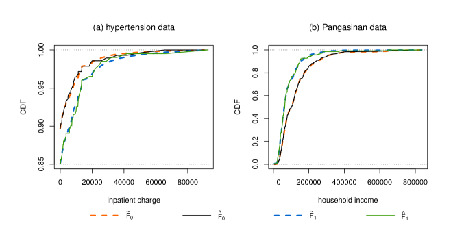
Figure 1: Fitted population distributions for real datasets. $\hat{F}_{0}$ and $\hat{F}_{1}$: fitted CDFs under the DRM; $\tilde{F}_{0}$ and $\tilde{F}_{1}$: empirical CDFs.

We apply the methods discussed in Sections 3.1 and 3.2 to this dataset. Table 9 presents the point estimates, and Table 10 shows the lower bound (LB), upper bound (UB), and length of the 95% CIs. The estimates of $\mathcal{G}_{0}$, $\mathcal{G}_{1}$, and $\mathcal{G}_{0}-\mathcal{G}_{1}$ for all three methods are very close. In particular, the EMP and JEL estimates are almost the same. The estimates of $\mathcal{G}_{0}$ and $\mathcal{G}_{1}$ are greater than 0.93, indicating the large inequality of the inpatient charge for patients with uncomplicated hypertension; the high proportion of zero values contributes to this. All the methods give similar 95% CIs for $\mathcal{G}_{0}$. The 95% CIs for $\mathcal{G}_{1}$ and $\mathcal{G}_{0}-\mathcal{G}_{1}$ for NA-DRM and BT-DRM are the shortest. All the CIs for $\mathcal{G}_{0}-\mathcal{G}_{1}$ contain 0, which suggests no significant difference between the inequality of the inpatient charge for female and male patients at the 95% confidence level.

Table 9: Point estimates of Gini indices and their difference (hypertension data).

	$\mathcal{G}_{0}$ (male)	$\mathcal{G}_{1}$ (female)	$\mathcal{G}_{0}-\mathcal{G}_{1}$
EMP	0.959	0.933	0.026
JEL	0.959	0.933	0.026
DRM	0.956	0.934	0.022

Table 10: 95% CIs for the two Gini indices and their difference (hypertension data).

	$\mathcal{G}_{0}$ (male)			$\mathcal{G}_{1}$ (female)			$\mathcal{G}_{0}-\mathcal{G}_{1}$
	LB	UB	Length	LB	UB	Length	LB	UB	Length
NA-EMP	0.942	0.977	0.035	0.902	0.964	0.062	-0.009	0.062	0.071
BT-EMP	0.936	0.974	0.039	0.888	0.959	0.071	-0.013	0.066	0.078
EL	0.941	0.975	0.034	0.903	0.961	0.058	–	–	–
BT-EL	0.938	0.976	0.038	0.897	0.966	0.068	–	–	–
JEL	0.942	0.980	0.038	0.904	0.967	0.063	-0.017	0.069	0.086
AJEL	0.942	0.981	0.039	0.904	0.967	0.064	-0.018	0.069	0.087
NA-DRM	0.938	0.974	0.036	0.906	0.961	0.056	-0.009	0.054	0.063
BT-DRM	0.934	0.972	0.038	0.901	0.957	0.056	-0.007	0.048	0.055

The second dataset comes from the 1997 Family and Income and Expenditure Survey conducted by the Philippine Statistics Authority; the metadata is available in the R package ineq. The province of Pangasinan is located in the Ilocos Region of Luzon. The dataset contains household incomes from different areas of Pangasinan: urban (Sample 0) and rural (Sample 1). Sample 0 has 245 observations and sample 1 has 138 observations. All the incomes are positive.

The skewness of the dataset suggests setting $\boldsymbol{q}(x)=\log(x)$ in the DRM (3). The goodness-of-fit test of Qin & Zhang (1997) gives a p-value 0.607. Hence, there is no strong evidence to reject the choice of $\boldsymbol{q}(x)=\log(x)$. Figure 1(b) also shows that the DRM with $\boldsymbol{q}(x)=\log(x)$ fits the data well.

We use all the methods of Sections 3.1 and 3.2 to analyze the dataset and summarize the results in Tables 11 and 12. The EMP and JEL methods give similar estimates of $\mathcal{G}_{0}$, $\mathcal{G}_{1}$, and $\mathcal{G}_{0}-\mathcal{G}_{1}$. The DRM estimate of $\mathcal{G}_{0}$ is comparable to the other estimates, while the DRM estimate of $\mathcal{G}_{1}$ is smaller than the others. Hence, the DRM estimate of $\mathcal{G}_{0}-\mathcal{G}_{1}$ is larger. All the methods give similar results for the 95% CIs for $\mathcal{G}_{0}$. The 95% CIs for $\mathcal{G}_{1}$ and $\mathcal{G}_{0}-\mathcal{G}_{1}$ by NA-DRM and BT-DRM are significantly shorter than the other CIs. This is strong evidence that our method helps to utilize information across the two samples and effectively improves inference when sample sizes are small or moderate. We do not reject the hypothesis that the income inequalities of urban and rural households are the same, since all the 95% CIs for $\mathcal{G}_{0}-\mathcal{G}_{1}$ contain 0.

Table 11: Point estimates of Gini indices and their difference (Pangasinan data).

	$\mathcal{G}_{0}$ (urban)	$\mathcal{G}_{1}$ (rural)	$\mathcal{G}_{0}-\mathcal{G}_{1}$
EMP	0.393	0.394	-0.001
JEL	0.391	0.389	0.002
DRM	0.399	0.371	0.028

Table 12: 95% CIs for the two Gini indices and their difference (Pangasinan data).

	$\mathcal{G}_{0}$ (urban)			$\mathcal{G}_{1}$ (rural)			$\mathcal{G}_{0}-\mathcal{G}_{1}$
	LB	UB	Length	LB	UB	Length	LB	UB	Length
NA-EMP	0.354	0.433	0.079	0.332	0.455	0.123	-0.074	0.073	0.146
BT-EMP	0.356	0.441	0.085	0.338	0.481	0.143	-0.085	0.068	0.153
EL	0.354	0.433	0.079	0.333	0.456	0.123	–	–	–
BT-EL	0.353	0.434	0.080	0.335	0.455	0.120	–	–	–
JEL	0.356	0.436	0.081	0.339	0.466	0.127	-0.083	0.070	0.153
AJEL	0.355	0.437	0.081	0.338	0.467	0.129	-0.084	0.071	0.154
NA-DRM	0.361	0.436	0.075	0.343	0.399	0.055	-0.003	0.059	0.062
BT-DRM	0.359	0.443	0.084	0.343	0.403	0.060	-0.006	0.057	0.063

5 Concluding Remarks

We have proposed new semiparametric inference procedures for the Gini indices of two semicontinuous populations. Under the mixture model (1) and the DRM (3), we proposed the MELEs of the Gini indices $\mathcal{G}_{0}$ and $\mathcal{G}_{1}$ and established the asymptotic normality of the MELEs. Our methods are applicable whether or not there are excess zero values. We showed numerically and theoretically that our MELEs are more efficient than fully nonparametric estimators. We also explored the asymptotic properties of a general function of two Gini indices, and used the difference of the two Gini indices as an illustrating example. We used the asymptotic results to construct CIs and perform hypothesis tests for $\mathcal{G}_{0}$, $\mathcal{G}_{1}$, and $\mathcal{G}_{0}-\mathcal{G}_{1}$. Simulation studies demonstrated that the CIs under the DRM have superior performance in terms of coverage accuracy and average length. Moreover, our method has a higher testing power than existing methods.

ELR-based CIs are range-preserving. It would be interesting to construct ELR-based CIs for Gini indices under the DRM, but the theoretical development may be technically challenging. Qin et al. (2010) investigated inference on the Gini index of a population under stratified random sampling. We could use the DRM to link the distributions of the subpopulations in all strata and then develop an inference procedure for the Gini index of the whole population. Correlated data is also of interest: Peng (2011) and Wang & Zhao (2016) compared the Gini indices of paired data. The DRM would be useful for modeling the marginal distributions of paired data and improving the efficiency of the estimation of the Gini indices. We leave these topics to future research.

Supplementary material for
“Semiparametric inference on Gini indices of two semicontinuous populations under density ratio models”

This document of supplementary material provides further details for the paper entitled “Semiparametric inference on Gini indices of two semicontinuous populations under density ratio models”. It contains the proofs of Theorems 1–4 in the main paper and additional simulation results. The basic setting and some useful lemmas are presented in Section 1. The proofs and technical details for Theorems 1–4 are given in Sections 2–5. Section 6 contains some additional simulation results.

1 The basic setting and useful lemmas

Recall that

$$(X_{i1},\cdots,X_{in_{i}})\sim F_{i}(x)=\nu_{i}I(x\geq 0)+(1-\nu_{i})I(x>0)G_{i}(x),\leavevmode\nobreak\ \leavevmode\nobreak\ \mbox{for\leavevmode\nobreak\ }\leavevmode\nobreak\ i=0,1,$$ (S.1)

where $\nu_{i}$ is the proportion of zeros in sample $i$, $n_{i}$ is the sample size for sample $i$, $I(\cdot)$ is an indicator function, and $G_{i}(\cdot)$ is the cumulative distribution function (CDF) of the positive observations in sample $i$. We link $G_{0}(x)$ and $G_{1}(x)$ via a density ratio model (DRM):

$$dG_{1}(x)=\exp\{\alpha+\boldsymbol{\beta}^{\top}\boldsymbol{q}(x)\}dG_{0}(x)=\exp\{\boldsymbol{\theta}^{\top}\boldsymbol{Q}(x)\}dG_{0}(x)$$ (S.2)

for the unknown parameter $\boldsymbol{\theta}=(\alpha,\boldsymbol{\beta}^{\top})^{\top}$ and $\boldsymbol{Q}(x)=(1,\boldsymbol{q}(x)^{\top})^{\top}$ with $\boldsymbol{q}(x)$ a $d$-dimensional, prespecified, nontrivial basis function.

Recall that $n_{i0}$ and $n_{i1}$ are the (random) numbers of zero observations and positive observations, respectively, in sample $i=0,1$. Clearly, $n_{i}=n_{i0}+n_{i1}$, for $i=0,1$. Without loss of generality, we assume that the first $n_{i1}$ observations in group $i$, $X_{i1},\cdots,X_{in_{i1}}$, are positive, and the remaining $n_{i0}$ observations are 0. Let $n$ be the total (fixed) sample size, i.e., $n=n_{0}+n_{1}$.

We further let $\boldsymbol{\nu}=(\nu_{0},\nu_{1})^{\top}$. The maximum empirical likelihood estimators (MELEs) of $\boldsymbol{\nu}$ and $\boldsymbol{\theta}$ respectively maximize $\ell_{0}\left(\boldsymbol{\nu}\right)$ and $\ell_{1}(\boldsymbol{\theta})$, where

$$\ell_{0}\left(\boldsymbol{\nu}\right)=\sum_{i=0}^{1}\log\left\{\nu_{i}^{n_{i0}}\left(1-\nu_{i}\right)^{n_{i1}}\right\}$$

and

$$\ell_{1}(\boldsymbol{\theta})=-\sum_{i=0}^{1}\sum_{j=1}^{n_{i1}}\log\left\{1+\hat{\rho}[\exp\{\boldsymbol{\theta}^{\top}\boldsymbol{Q}(X_{ij})\}-1]\right\}+\sum_{j=1}^{n_{11}}\{\boldsymbol{\theta}^{\top}\boldsymbol{Q}(X_{1j})\}$$

with $\hat{\rho}={n_{11}}/{(n_{01}+n_{11})}$ being a random variable. That is,

$$\hat{\boldsymbol{\nu}}=\arg\max_{\mbox{\scriptsize\boldmath$\nu$}}\ell_{0}\left(\boldsymbol{\nu}\right)\leavevmode\nobreak\ \leavevmode\nobreak\ \mbox{ and }\leavevmode\nobreak\ \leavevmode\nobreak\ \hat{\boldsymbol{\theta}}=\arg\max_{\mbox{\scriptsize\boldmath$\theta$}}\ell_{1}(\boldsymbol{\theta}).$$ (S.3)

Once $\hat{\boldsymbol{\theta}}$ is obtained, we have

$$\hat{p}_{ij}=(n_{01}+n_{11})^{-1}\left\{1+\hat{\rho}[\exp\{\hat{\boldsymbol{\theta}}^{\top}\boldsymbol{Q}(X_{ij})\}-1]\right\}^{-1}.$$

Note that $\sum_{i=0}^{1}\sum_{j=1}^{n_{i1}}\hat{p}_{ij}=1$, which ensures that the MELE of $G_{0}(x)$ is a CDF. The MELEs of $G_{0}(x)$ and $G_{1}(x)$ for $x>0$ are

$$\hat{G}_{0}(x)=\sum_{i=0}^{1}\sum_{j=1}^{n_{i1}}\hat{p}_{ij}I(X_{ij}\leq x)\leavevmode\nobreak\ \leavevmode\nobreak\ \mbox{and}\leavevmode\nobreak\ \leavevmode\nobreak\ \hat{G}_{1}(x)=\sum_{i=0}^{1}\sum_{j=1}^{n_{i1}}\hat{p}_{ij}\exp\{\hat{\boldsymbol{\theta}}^{\top}\boldsymbol{Q}(X_{ij})\}I(X_{ij}\leq x).$$ (S.4)

For convenience of presentation, we recall and introduce some notation. We use $\boldsymbol{\nu}^{*}$ and $\boldsymbol{\theta}^{*}$ to denote the true values of $\boldsymbol{\nu}$ and $\boldsymbol{\theta}$. Let $\boldsymbol{\eta}=(\boldsymbol{\nu}^{\top},\rho,\boldsymbol{\theta}^{\top})^{\top}$, $w_{i}=n_{i}/n$ for $i=0,1$, and

$$\Delta^{*}=\sum_{i=0}^{1}w_{i}(1-\nu_{i}^{*}),\leavevmode\nobreak\ \rho^{*}=\frac{w_{1}(1-\nu_{1}^{*})}{\Delta^{*}},\leavevmode\nobreak\ \omega(x;\boldsymbol{\theta})=\exp\{\boldsymbol{\theta}^{\top}\boldsymbol{Q}(x)\},\leavevmode\nobreak\ \omega(x)=\omega(x;\boldsymbol{\theta}^{*}),$$

$$h(x)=1+\rho^{*}\{\omega(x)-1\},\leavevmode\nobreak\ h_{1}(x)=\rho^{*}\omega(x)/h(x),\leavevmode\nobreak\ h_{0}(x)=(1-\rho^{*})/h(x).$$

Note that $\omega(\cdot)$, $h(\cdot)$, $h_{0}(\cdot)$, and $h_{1}(\cdot)$ depend on $\boldsymbol{\theta}^{*}$ and/or $\rho^{*}$ and $h_{0}(x)+h_{1}(x)=1$. Henceforth, we use $\sum_{ij}$ and $\sum_{ls}$ to denote summation over the full range of data.

1.1 Alternative form of Gini index

According to David (1968), the Gini’s mean difference for sample $i$ can be equivalently expressed by

$$D_{i}=E|X_{i1}-X_{i2}|=2\int_{-\infty}^{\infty}\left\{2xF_{i}(x)-x\right\}dF_{i}(x).$$

Under model (S.1), $F_{i}(x)=\nu_{i}I(x\geq 0)+(1-\nu_{i})I(x>0)G_{i}(x)$. Then $D_{i}$ can be further written as

$$D_{i} = 2(1-\nu_{i})\int_{0}^{\infty}[2x\{\nu_{i}+(1-\nu_{i})G_{i}(x)\}-x]dG_{i}(x)$$

$$= 2(1-\nu_{i})\int_{0}^{\infty}x\{(2\nu_{i}-1)+(1-\nu_{i})2G_{i}(x)\}dG_{i}(x)$$

$$= 2(2\nu_{i}-1)\int_{0}^{\infty}x(1-\nu_{i})dG_{i}(x)+2(1-\nu_{i})^{2}\int_{0}^{\infty}\{2xG_{i}(x)\}dG_{i}(x)$$

$$= 2(2\nu_{i}-1)\mu_{i}+2(1-\nu_{i})^{2}\int_{0}^{\infty}\{2xG_{i}(x)\}dG_{i}(x).$$

Let $m_{i}=\int_{0}^{\infty}xdG_{i}(x)$ and $\psi_{i}=\int_{0}^{\infty}\{2xG_{i}(x)\}dG_{i}(x)$. We then have $\mu_{i}=(1-\nu_{i})m_{i}$ and

$$\mathcal{G}_{i}=\frac{D_{i}}{2\mu_{i}}=(2\nu_{i}-1)+(1-\nu_{i})\frac{\psi_{i}}{m_{i}}.$$

With the definition of $m_{i}$ and $\psi_{i}$, and the MELEs of CDFs $G_{i}$’s in (S.4), the MELEs of $m_{i}$ and $\psi_{i}$ are as follows:

$$\hat{m}_{0} = \sum_{i=0}^{1}\sum_{j=1}^{n_{i1}}\hat{p}_{ij}X_{ij},\leavevmode\nobreak\ \leavevmode\nobreak\ \leavevmode\nobreak\ \hat{m}_{1}=\sum_{i=0}^{1}\sum_{j=1}^{n_{i1}}\hat{p}_{ij}\omega(X_{ij};\hat{\boldsymbol{\theta}})X_{ij},$$

$$\hat{\psi}_{0} = \sum_{i=0}^{1}\sum_{j=1}^{n_{i1}}\hat{p}_{ij}\{2X_{ij}\hat{G}_{0}(X_{ij})\}=\sum_{i=0}^{1}\sum_{j=1}^{n_{i1}}\hat{p}_{ij}X_{ij}\left\{2\sum_{l=0}^{1}\sum_{s=1}^{n_{l1}}\hat{p}_{ls}I(X_{ls}\leq X_{ij})\right\},$$

$$\hat{\psi}_{1} = \sum_{i=0}^{1}\sum_{j=1}^{n_{i1}}\hat{p}_{ij}\omega(X_{ij};\hat{\boldsymbol{\theta}})\{2X_{ij}\hat{G}_{1}(X_{ij})\}$$

$$=\sum_{i=0}^{1}\sum_{j=1}^{n_{i1}}\hat{p}_{ij}\omega(X_{ij};\hat{\boldsymbol{\theta}})X_{ij}\left\{2\sum_{l=0}^{1}\sum_{s=1}^{n_{l1}}\hat{p}_{ls}\omega(X_{ls};\hat{\boldsymbol{\theta}})I(X_{ls}\leq X_{ij})\right\}.$$

The MELEs of the two Gini indices are given by

$$\hat{\mathcal{G}}_{i}=(2\hat{\nu}_{i}-1)+(1-\hat{\nu}_{i})\frac{\hat{\psi}_{i}}{\hat{m}_{i}}\leavevmode\nobreak\ \leavevmode\nobreak\ \leavevmode\nobreak\ \text{for}\leavevmode\nobreak\ i=0,1.$$ (S.5)

1.2 Some useful lemmas

We present several useful lemmas in preparation for the proofs in Sections 2–5. The first lemma considers the expectation of summations.

Lemma 1.

Suppose that $g(x)$ is an arbitrary vector-valued function. Let $E_{0}(\cdot)$ represent the expectation operator with respect to $G_{0}$ and $X$ be a random variable from $G$. Then

$$E\left\{\sum_{ij}g(X_{ij})I(X_{ij}>0)\right\}=\sum_{i=0}^{1}n_{i}{E}\{g(X_{i1})I(X_{i1}>0)\}=n\Delta^{*}E_{0}\{h(X)g(X)\}.$$

Proof.

Under the DRM ( S.2),

$$\sum_{i=0}^{1}n_{i}{E}\{g(X_{i1})I(X_{i1}>0)\}=n_{0}(1-\nu_{0}^{*})E_{0}\{g(X)\}+n_{1}(1-\nu_{1}^{*})E_{0}\{\omega(X)g(X)\}.$$

Since $w_{i}=n_{i}/n$ and using the definitions of $\Delta^{*}$ and $\rho^{*}$, we further have

$$E\left\{\sum_{ij}g(X_{ij})I(X_{ij}>0)\right\} = nw_{0}(1-\nu_{0}^{*})E_{0}\{g(X)\}+nw_{1}(1-\nu_{1}^{*})E_{0}\{\omega(X)g(X)\}$$

$$= n\Delta^{*}E_{0}\{(1-\rho^{*})g(X)\}+n\Delta^{*}E_{0}[\rho^{*}\omega(X)g(X)].$$

Recalling that $h(x)=1+\rho^{*}\{\omega(x)-1\}=(1-\rho^{*})+\rho^{*}\omega(x)$, we have

$$E\left\{\sum_{ij}g(X_{ij})I(X_{ij}>0)\right\}=n\Delta^{*}E_{0}\{h(X)g(X)\}.$$

This completes the proof. $\hfill\square$

Yuan et al. (2020) define a general parameter vector $\boldsymbol{\gamma}$ of length $p$:

$$\boldsymbol{\gamma}=\int_{0}^{\infty}\boldsymbol{u}(x;\boldsymbol{\nu},\boldsymbol{\theta})dG_{0}(x),$$ (S.6)

where $\boldsymbol{u}(x;\boldsymbol{\nu},\boldsymbol{\theta})=\left(u_{1}(x;\boldsymbol{\nu},\boldsymbol{\theta}),\ldots,u_{p}(x;\boldsymbol{\nu},\boldsymbol{\theta})\right)^{\top}$ is a given $p\times 1$ dimensional function. The MELE of $\boldsymbol{\gamma}$ is given by

$$\hat{\boldsymbol{\gamma}}=\sum_{i=0}^{1}\sum_{j=1}^{n_{i1}}\hat{p}_{ij}\boldsymbol{u}(X_{ij};\hat{\boldsymbol{\nu}},\hat{\boldsymbol{\theta}}).$$ (S.7)

The following lemmas provide the approximation of the MELE $\hat{\boldsymbol{\gamma}}$ and its asymptotic property. These lemmas help to develop the asymptotic property of the MELEs of the Gini indices.

Lemma 2.

Assume that Conditions C1–C3 are satisfied and the true value $\nu_{i}^{*}\in(0,1)$ for $i=0,1$. Let $\boldsymbol{\gamma}^{*}$ be the true value of $\boldsymbol{\gamma}$ and $\boldsymbol{\eta}^{*}=(\boldsymbol{\nu}^{*\top},\rho^{*},\boldsymbol{\theta}^{*\top})^{\top}$. Then

$$\hat{\boldsymbol{\gamma}} = \frac{1}{n\Delta^{*}}\sum_{ij}\frac{\boldsymbol{u}(x;\boldsymbol{\nu}^{*},\boldsymbol{\theta}^{*})}{h(X_{ij})}I(X_{ij}>0)+\boldsymbol{C}(\hat{\boldsymbol{\eta}}-\boldsymbol{\eta}^{*})+o_{p}(n^{-1/2}),$$ (S.8)

where $\boldsymbol{C}=(\boldsymbol{C}_{\mbox{\scriptsize\boldmath$\nu$}},C_{\rho},\boldsymbol{C}_{\mbox{\scriptsize\boldmath$\theta$}})$ with

$$\boldsymbol{C}_{\mbox{\scriptsize\boldmath$\nu$}} = E_{0}\left\{\frac{\partial\boldsymbol{u}(X;\boldsymbol{\nu}^{*},\boldsymbol{\theta}^{*})}{\partial\boldsymbol{\nu}}\right\}+\left(\frac{w_{0}\boldsymbol{\gamma}^{*}}{\Delta^{*}},\frac{w_{1}\boldsymbol{\gamma}^{*}}{\Delta^{*}}\right),$$

$$\boldsymbol{C}_{\rho} = -E_{0}\left\{\frac{\boldsymbol{u}(X;\boldsymbol{\nu}^{*},\boldsymbol{\theta}^{*})\{\omega(X)-1\}}{h(X)}\right\},$$

$$\boldsymbol{C}_{\mbox{\scriptsize\boldmath$\theta$}} = E_{0}\left\{\frac{\partial\boldsymbol{u}(X;\boldsymbol{\nu}^{*},\boldsymbol{\theta}^{*})}{\partial\boldsymbol{\theta}}\right\}-E_{0}\left\{h_{1}(X)\boldsymbol{u}(X;\boldsymbol{\nu}^{*},\boldsymbol{\theta}^{*})\boldsymbol{Q}(X)^{\top}\right\}.$$

Lemma 3.

Under the conditions of Lemma 2, as $n\to\infty$, $\sqrt{n}(\hat{\boldsymbol{\gamma}}-\boldsymbol{\gamma}^{*})\to N({\bf 0},\boldsymbol{\Gamma})$ in distribution, where

$$\boldsymbol{\Gamma} = \frac{1}{\Delta^{*}}E_{0}\left\{\frac{\boldsymbol{u}(X;\boldsymbol{\nu}^{*},\boldsymbol{\theta}^{*})\boldsymbol{u}(X;\boldsymbol{\nu}^{*},\boldsymbol{\theta}^{*})^{\top}}{h(X)}\right\}-\frac{\boldsymbol{\gamma}^{*}\boldsymbol{\gamma}^{*\top}}{\Delta^{*}}$$

$$+\mathcal{M}_{1}\boldsymbol{A}_{\mbox{\scriptsize\boldmath$\nu$}}^{-1}\mathcal{M}_{1}^{\top}-\frac{\mathcal{M}_{2}\mathcal{M}_{2}^{\top}}{\Delta^{*}\rho^{*}(1-\rho^{*})}+\mathcal{M}_{3}\boldsymbol{A}_{\mbox{\scriptsize\boldmath$\theta$}}^{-1}\mathcal{M}_{3}^{\top},$$

with $\boldsymbol{A}_{\mbox{\scriptsize\boldmath$\nu$}}=\rm\mbox{diag}\left\{\frac{w_{0}}{\nu_{0}^{*}(1-\nu_{0}^{*})},\frac{w_{1}}{\nu_{1}^{*}(1-\nu_{1}^{*})}\right\},\leavevmode\nobreak\ \boldsymbol{A}_{\mbox{\scriptsize\boldmath$\theta$}}=\Delta^{*}(1-\rho^{*})E_{0}\left\{h_{1}(X)\boldsymbol{Q}(X)\boldsymbol{Q}(X)^{\top}\right\}$, and

$$\mathcal{M}_{1} = E_{0}\left\{\frac{\partial\boldsymbol{u}(X;\boldsymbol{\nu}^{*},\boldsymbol{\theta}^{*})}{\partial\boldsymbol{\nu}}\right\},$$

$$\mathcal{M}_{2} = E_{0}\left[\left\{\partial\boldsymbol{u}(X;\boldsymbol{\nu}^{*},\boldsymbol{\theta}^{*})/\partial\boldsymbol{\theta}\right\}\boldsymbol{e}\right]-\rho^{*}\boldsymbol{\gamma}^{*},$$

$$\mathcal{M}_{3} = E_{0}\left\{\partial\boldsymbol{u}(X;\boldsymbol{\nu}^{*},\boldsymbol{\theta}^{*})/\partial\boldsymbol{\theta}-h_{1}(X)\boldsymbol{u}(X;\boldsymbol{\nu}^{*},\boldsymbol{\theta}^{*})\boldsymbol{Q}(X)^{\top}\right\}.$$

Proof.

The proofs of Lemmas 2 and 3 can be found in the supplementary material of Yuan et al. (2020). $\hfill\square$

2 Proof of Theorem 1

2.1 Approximations of $\hat{\psi}_{0}$ and $\hat{\psi}_{1}$

To develop the asymptotic properties of $(\hat{\mathcal{G}}_{0},\hat{\mathcal{G}}_{1})$, we first find the linear approximations of $\hat{\psi}_{0}$ and $\hat{\psi}_{1}$. We start with $\hat{\psi}_{0}$.

Recall that

$$\hat{p}_{ij} = \frac{1}{n_{01}+n_{11}}\left\{1+\hat{\rho}[\exp\{\hat{\boldsymbol{\theta}}^{\top}\boldsymbol{Q}(X_{ij})\}-1]\right\}^{-1}$$

$$= \frac{1}{nw_{0}(1-\hat{\nu}_{0})+nw_{1}(1-\hat{\nu}_{1})}\left\{1+\hat{\rho}[\exp\{\hat{\boldsymbol{\theta}}^{\top}\boldsymbol{Q}(X_{ij})\}-1]\right\}^{-1}.$$

The MELE $\hat{\psi}_{0}$ is then given by

$$\hat{\psi}_{0} = \{nw_{0}(1-\hat{\nu}_{0})+nw_{1}(1-\hat{\nu}_{1})\}^{-2}\times$$

$$\sum_{ij}\sum_{ls}\frac{2I(X_{ls}\leq X_{ij})X_{ij}\cdot I(X_{ij}>0)I(X_{ls}>0)}{\left\{1+\hat{\rho}[\exp\{\hat{\boldsymbol{\theta}}^{\top}\boldsymbol{Q}(X_{ij})\}-1]\right\}\left\{1+\hat{\rho}[\exp\{\hat{\boldsymbol{\theta}}^{\top}\boldsymbol{Q}(X_{ls})\}-1]\right\}}.$$

Note that $\hat{\psi}_{0}$ is a function of $\boldsymbol{\eta}$, and hence we define

$$\psi_{0}(\boldsymbol{\eta}) = \{nw_{0}(1-\nu_{0})+nw_{1}(1-\nu_{1})\}^{-2}\times$$

$$\sum_{ij}\sum_{ls}\frac{2I(X_{ls}\leq X_{ij})X_{ij}\cdot I(X_{ij}>0)I(X_{ls}>0)}{\left\{1+{\rho}[\exp\{\boldsymbol{\theta}^{\top}\boldsymbol{Q}(X_{ij})\}-1]\right\}\left\{1+{\rho}[\exp\{\boldsymbol{\theta}^{\top}\boldsymbol{Q}(X_{ls})\}-1]\right\}}.$$

We then have $\hat{\psi}_{0}=\psi_{0}(\hat{\boldsymbol{\eta}})$. With the definition of $\Delta^{*}$ and $h(x)$, we have

$$\psi_{0}(\boldsymbol{\eta}^{*})=\frac{1}{(n\Delta^{*})^{2}}\sum_{ij}\sum_{ls}\frac{2I(X_{ls}\leq X_{ij})X_{ij}}{h(X_{ij})h(X_{ls})}I(X_{ij}>0)I(X_{ls}>0)$$

and $E_{0}\{\psi_{0}(\boldsymbol{\eta}^{*})\}=\psi_{0}$.

By Theorem 1 of Yuan et al. (2020), we have $\hat{\boldsymbol{\eta}}=\boldsymbol{\eta}^{*}+O_{p}(n^{-1/2})$. Applying the first-order Taylor expansion gives

$$\psi_{0}(\hat{\boldsymbol{\eta}})=\psi_{0}(\boldsymbol{\eta}^{*})+\left\{\frac{\partial\psi_{0}(\boldsymbol{\eta}^{*})}{\partial\boldsymbol{\eta}}\right\}^{\top}(\hat{\boldsymbol{\eta}}-\boldsymbol{\eta}^{*})+o_{p}(n^{-1/2}).$$ (S.9)

Define

$$U(a,b) = \frac{I(b\leq a)a}{h(a)h(b)}I(a>0)I(b>0),\leavevmode\nobreak\ \leavevmode\nobreak\ \leavevmode\nobreak\ V_{nil}=\frac{1}{n_{i}}\frac{1}{n_{l}}\sum_{j=1}^{n_{i}}\sum_{s=1}^{n_{l}}U(X_{ij},X_{ls}),$$

$$V_{ni} = \frac{1}{n_{i}^{2}}\sum_{j=1}^{n_{i}}\sum_{s=1}^{n_{i}}2U(X_{ij},X_{is})=\frac{1}{n_{i}^{2}}\sum_{j=1}^{n_{i}}\sum_{s=1}^{n_{i}}\left\{U(X_{ij},X_{is})+U(X_{is},X_{ij})\right\},$$

for $i,l\in\{0,1\}$ and $i\neq l$. We then rewrite $\psi_{0}(\boldsymbol{\eta}^{*})$ as

$$\psi_{0}(\boldsymbol{\eta}^{*}) = \frac{1}{(\Delta^{*})^{2}}\sum_{i=0}^{1}\sum_{l=0}^{1}w_{i}w_{l}\frac{1}{n_{i}}\frac{1}{n_{l}}\sum_{j=1}^{n_{i}}\sum_{s=1}^{n_{l}}2U(X_{ij},X_{ls})$$

$$= \frac{1}{(\Delta^{*})^{2}}\left\{\sum_{i=0}^{1}w_{i}^{2}V_{ni}+\sum_{i=0}^{1}\sum_{l\neq i}w_{i}w_{l}2V_{nil}\right\}.$$

Note that $V_{ni}$ is a von Mises statistic (Mises, 1947). We denote the associated U-statistic by

$$U_{ni}=\binom{n_{i}}{2}^{-1}\sum_{1\leq j<s\leq n_{i}}\left\{U(X_{ij},X_{is})+U(X_{is},X_{ij})\right\}.$$

According to Serfling (1980), the projection of $U_{ni}$ is defined as

$$\hat{U}_{ni}=E\{U_{i}(X_{i1})\}+\frac{2}{n_{i}}\sum_{j=1}^{n_{i}}\left[U_{i}(X_{ij})-E\{U_{i}(X_{i1})\}\right],$$

where $U_{i}(a)=E\{U(a,X_{i1})+U(X_{i1},a)\}$. It follows from Serfling (1980, p. 190  &  p. 206) that under Condition C4,

$$\sqrt{n_{i}}(\hat{U}_{ni}-U_{ni})=o_{p}(1)\leavevmode\nobreak\ \leavevmode\nobreak\ \mbox{and}\sqrt{n_{i}}(V_{ni}-U_{ni})=o_{p}(1).$$

This leads to

$$V_{ni}=E\{U_{i}(X_{i1})\}+\frac{2}{n_{i}}\sum_{j=1}^{n_{i}}\left[U_{i}(X_{ij})-E\{U_{i}(X_{i1})\}\right]+o_{p}(n^{-1/2}).$$

When $l\neq i$, $V_{nil}$ is a two-sample U-statistic. Define $U_{il}=E\{U(X_{i1},X_{l1})\}$, $U_{il10}(a)=E\{U(a,X_{l1})\}-U_{il}$, and $U_{il01}(a)=E\{U(X_{i1},a)\}-U_{il}$. From Theorem 12.6 in Van der Vaart (2000), we have

$$V_{nil}=U_{il}+\frac{1}{n_{i}}\sum_{j=1}^{n_{i}}U_{il10}(X_{ij})+\frac{1}{n_{l}}\sum_{s=1}^{n_{l}}U_{il01}(X_{ls})+o_{p}(n^{-1/2}).$$

Since

$$E\{U_{i}(X_{i1})\}=2E\{U(X_{i1},X_{i1})\}=2U_{ii}$$

$$U_{i}(a)-E\{U_{i}(X_{i1})\}=U_{ii10}(a)+U_{ii01}(a),$$

we have

$$V_{ni}=2\left\{U_{ii}+\frac{1}{n_{i}}\sum_{j=1}^{n_{i}}U_{ii10}(X_{ij})+\frac{1}{n_{i}}\sum_{j=1}^{n_{i}}U_{ii01}(X_{ij})\right\}+o_{p}(n^{-1/2}).$$

Hence,

$$\psi_{0}(\boldsymbol{\eta}^{*}) = \frac{2}{(\Delta^{*})^{2}}\sum_{i=0}^{1}\sum_{l=0}^{1}w_{i}w_{l}U_{il}+\frac{2}{(\Delta^{*})^{2}}\sum_{i=0}^{1}\sum_{l=0}^{1}w_{i}w_{l}\frac{1}{n_{i}}\sum_{j=1}^{n_{i}}U_{il10}(X_{ij})$$ (S.10)

$$+\frac{2}{(\Delta^{*})^{2}}\sum_{i=0}^{1}\sum_{l=0}^{1}w_{i}w_{l}\frac{1}{n_{l}}\sum_{s=1}^{n_{l}}U_{il01}(X_{ls})+o_{p}(n^{-1/2})$$

$$= \frac{2}{(n\Delta^{*})^{2}}\sum_{i=0}^{1}\sum_{l=0}^{1}n_{i}n_{l}U_{il}+\frac{2}{(n\Delta^{*})^{2}}\sum_{i=0}^{1}\sum_{l=0}^{1}n_{l}\sum_{j=1}^{n_{i}}U_{il10}(X_{ij})$$

$$+\frac{2}{(n\Delta^{*})^{2}}\sum_{i=0}^{1}\sum_{l=0}^{1}n_{i}\sum_{s=1}^{n_{l}}U_{il01}(X_{ls})+o_{p}(n^{-1/2}).$$

We now simplify each term in (S.10). With Lemma 1 and the definition of $U_{il}$, we have

$$\sum_{l=0}^{1}n_{l}E\{U(X_{i1},X_{l1})|X_{i1}\} = \sum_{l=0}^{1}n_{l}E\left\{\frac{I(X_{l1}\leq X_{i1})X_{i1}}{h(X_{i1})h(X_{l1})}I(X_{i1}>0)I(X_{l1}>0)|X_{i1}\right\}$$

$$= n\Delta^{*}\frac{X_{i1}}{h(X_{i1})}I(X_{i1}>0)E_{0}\left\{I(X\leq X_{i1})\right\}$$

$$= n\Delta^{*}\frac{X_{i1}G_{0}(X_{i1})}{h(X_{i1})}I(X_{i1}>0).$$

Hence,

$$\frac{2}{(n\Delta^{*})^{2}}\sum_{i=0}^{1}\sum_{l=0}^{1}n_{i}n_{l}U_{il} = \frac{2}{(n\Delta^{*})^{2}}\sum_{i=0}^{1}n_{i}E\left[\sum_{l=0}^{1}n_{l}E\{U(X_{i1},X_{l1})|X_{i}\}\right]$$

$$= \frac{2}{n\Delta^{*}}\sum_{i=0}^{1}n_{i}E\left\{\frac{X_{i1}G_{0}(X_{i1})}{h(X_{i1})}I(X_{i1}>0)\right\}.$$

Using the result in Lemma 1, we have

$$\frac{2}{(n\Delta^{*})^{2}}\sum_{i=0}^{1}\sum_{l=0}^{1}n_{i}n_{l}U_{il}=2E_{0}\{XG_{0}(X)\}=\psi_{0}.$$

We move to the second term of $\psi_{0}(\boldsymbol{\eta}^{*})$ in (S.10). Recall that

$$U_{il10}(a)=E\{U(a,X_{l1})\}-E\{U(X_{i1},X_{l1})\}.$$

We then have

$$\sum_{l=0}^{1}n_{l}U_{il10}(X_{ij}) = \sum_{l=0}^{1}n_{l}\left\{E\{U(X_{ij},X_{l1})|X_{ij}\}-E[E\{U(X_{ij},X_{l1})|X_{ij}\}]\right\}$$

$$= n\Delta^{*}\left[\frac{X_{ij}G_{0}(X_{ij})}{h(X_{ij})}I(X_{ij}>0)-E\left\{\frac{X_{ij}G_{0}(X_{ij})}{h(X_{ij})}I(X_{ij}>0)\right\}\right].$$

This leads to

$$\frac{2}{(n\Delta^{*})^{2}}\sum_{i=0}^{1}\sum_{l=0}^{1}n_{l}\sum_{j=1}^{n_{i}}U_{il10}(X_{ij})$$

$$= \frac{2}{n\Delta^{*}}\sum_{ij}\left[\frac{X_{ij}G_{0}(X_{ij})}{h(X_{ij})}I(X_{ij}>0)-E\left\{\frac{X_{ij}G_{0}(X_{ij})}{h(X_{ij})}I(X_{ij}>0)\right\}\right]$$

$$= \frac{2}{n\Delta^{*}}\sum_{ij}\frac{I(X_{ij}>0)}{h(X_{ij})}X_{ij}G_{0}(X_{ij})-\psi_{0}.$$

Similarly, with the definition of $U_{il01}(a)$, we have

$$\sum_{i=0}^{1}n_{i}U_{il01}(X_{ls}) = \sum_{i=0}^{1}n_{i}\left\{E\{U(X_{i1},X_{ls})|X_{ls}\}-E[E\{U(X_{i1},X_{ls})|X_{ls}\}]\right\}.$$

Note that

$$\sum_{i=0}^{1}n_{i}E\{U(X_{i1},X_{ls})|X_{ls}\} = \sum_{i=0}^{1}n_{i}E\left\{\frac{I(X_{ls}\leq X_{i1})X_{i1}}{h(X_{i1})h(X_{ls})}I(X_{i1}>0)I(X_{ls}>0)|X_{ls}\right\}$$

$$= n\Delta^{*}\frac{I(X_{ls}>0)}{h(X_{ls})}E\left\{XI(X_{ls}\leq X)\right\}$$

$$= n\Delta^{*}\frac{I(X_{ls}>0)}{h(X_{ls})}\int_{X_{ls}}^{\infty}xdG_{0}(x).$$

Together with the result of Lemma 1, we have

$$\frac{2}{(n\Delta^{*})^{2}}\sum_{i=0}^{1}\sum_{l=0}^{1}n_{i}\sum_{s=1}^{n_{l}}U_{il01}(X_{ls})$$

$$= \frac{2}{n\Delta^{*}}\sum_{ls}\left[\frac{I(X_{ls}>0)}{h(X_{ls})}\int_{X_{ls}}^{\infty}xdG_{0}(x)-E\left\{\frac{I(X_{ls}>0)}{h(X_{ls})}\int_{X_{ls}}^{\infty}xdG_{0}(x)\right\}\right]$$

$$= \frac{2}{n\Delta^{*}}\sum_{ls}\frac{I(X_{ls}>0)}{h(X_{ls})}\int_{X_{ls}}^{\infty}xdG_{0}(x)-\psi_{0}.$$

For $a>0$, we define the function

$$H_{0}(a)=\left\{aG_{0}(a)+\int_{a}^{\infty}xdG_{0}(x)\right\}.$$

The approximation of $\psi_{0}(\boldsymbol{\eta}^{*})$ is then given by

$$\psi_{0}(\boldsymbol{\eta}^{*})=\frac{1}{n\Delta^{*}}\sum_{ij}\frac{I(X_{ij}>0)}{h(X_{ij})}\cdot\{2H_{0}(X_{ij})\}-\psi_{0}+o_{p}(n^{-1/2}).$$

We also need the first derivative of $\psi_{0}(\boldsymbol{\eta})$ when finding the approximation of $\psi_{0}(\hat{\boldsymbol{\eta}})$. We take the first derivative of $\psi_{0}(\boldsymbol{\eta})$ with respect to $\boldsymbol{\eta}$ and evaluate the derivative at the true value $\boldsymbol{\eta}^{*}$. This leads to

$$\frac{\partial\psi_{0}(\boldsymbol{\eta}^{*})}{\partial\boldsymbol{\nu}} = \frac{2}{\Delta^{*}}\psi_{0}(\boldsymbol{\eta}^{*})\left(\begin{array}[]{c}w_{0}\\ w_{1}\end{array}\right),$$

$$\frac{\partial\psi_{0}(\boldsymbol{\eta}^{*})}{\partial\rho} = -\frac{2}{(n\Delta^{*})^{2}}\sum_{ij}\sum_{ls}\left\{\frac{\omega(X_{ij})-1}{h(X_{ij})^{2}h(X_{ls})}+\frac{\omega(X_{ls})-1}{h(X_{ij})h(X_{ls})^{2}}\right\}$$

$$\times I(X_{ls}\leq X_{ij})X_{ij}I(X_{ij}>0)I(X_{ls}>0),$$

$$\frac{\partial\psi_{0}(\boldsymbol{\eta}^{*})}{\partial\boldsymbol{\theta}} = -\frac{2}{(n\Delta^{*})^{2}}\sum_{ij}\sum_{ls}\left\{\frac{\rho^{*}\omega(X_{ij})\boldsymbol{Q}(X_{ij})}{h(X_{ij})^{2}h(X_{ls})}+\frac{\rho^{*}\omega(X_{ls})\boldsymbol{Q}(X_{ls})}{h(X_{ij})h(X_{ls})^{2}}\right\}$$

$$\times I(X_{ls}\leq X_{ij})X_{ij}I(X_{ij}>0)I(X_{ls}>0),$$

$$= -\frac{2}{(n\Delta^{*})^{2}}\sum_{ij}\sum_{ls}\left\{h_{1}(X_{ij})\boldsymbol{Q}(X_{ij})+h_{1}(X_{ls})\boldsymbol{Q}(X_{ls})\right\}$$

$$\times\frac{I(X_{ls}\leq X_{ij})X_{ij}I(X_{ij}>0)I(X_{ls}>0)}{h(X_{ij})h(X_{ls})}.$$

By the law of large numbers, we have

$$\frac{\partial\psi_{0}(\boldsymbol{\eta}^{*})}{\partial\boldsymbol{\eta}}=E\left\{\frac{\partial\psi_{0}(\boldsymbol{\eta}^{*})}{\partial\boldsymbol{\eta}}\right\}+o_{p}(1)=\boldsymbol{C}_{0}+o_{p}(1),$$

with $\boldsymbol{C}_{0}=(\boldsymbol{C}_{0\mbox{\scriptsize\boldmath$\nu$}}^{\top},\boldsymbol{C}_{0\rho},\boldsymbol{C}_{0\mbox{\scriptsize\boldmath$\theta$}}^{\top})^{\top}$.

Since $E\{\psi_{0}(\boldsymbol{\eta}^{*})\}=\psi_{0}$, we have

$$\boldsymbol{C}_{0\mbox{\scriptsize\boldmath$\nu$}}=\frac{2\psi_{0}}{\Delta^{*}}(w_{0},w_{1})^{\top}.$$

For $\boldsymbol{C}_{0\rho}$,

$$\boldsymbol{C}_{0\rho} = E\left\{\frac{\partial\psi_{0}(\boldsymbol{\eta}^{*})}{\partial\rho}\right\}$$

$$= -\frac{2}{(n\Delta^{*})^{2}}E\left[\sum_{ij}E\left\{\sum_{ls}\frac{\omega(X_{ij})-1}{h(X_{ij})^{2}h(X_{ls})}I(X_{ls}\leq X_{ij})X_{ij}I(X_{ij}>0)I(X_{ls}>0)|X_{ij}\right\}\right]$$

$$-\frac{2}{(n\Delta^{*})^{2}}E\left[\sum_{ls}E\left\{\sum_{ij}\frac{\omega(X_{ls})-1}{h(X_{ij})h(X_{ls})^{2}}I(X_{ls}\leq X_{ij})X_{ij}I(X_{ij}>0)I(X_{ls}>0)|X_{ls}\right\}\right]$$

$$= -\frac{2}{n\Delta^{*}}E\left[\sum_{ij}\frac{\omega(X_{ij})-1}{h(X_{ij})^{2}}X_{ij}I(X_{ij}>0)G_{0}(x)\right]$$

$$-\frac{2}{n\Delta^{*}}E\left[\sum_{ls}\frac{\omega(X_{ls})-1}{h(X_{ls})^{2}}I(X_{ls}>0)E_{0}\left\{I(X_{ls}\leq X)X\right\}\right]$$

$$= -\frac{2}{n\Delta^{*}}E\left[\sum_{ij}\frac{\omega(X_{ij})-1}{h(X_{ij})^{2}}I(X_{ij}>0)H_{0}(X_{ij})\right]$$

$$= -2E_{0}\left\{\frac{H_{0}(X)\{\omega(X)-1\}}{h(X)}\right\}.$$

The expression for $\boldsymbol{C}_{0\mbox{\scriptsize\boldmath$\theta$}}$ can be found in a similar manner:

$$\boldsymbol{C}_{0\mbox{\scriptsize\boldmath$\theta$}}=-2E_{0}\left\{h_{1}(X)H_{0}(X)\boldsymbol{Q}(X)\right\}.$$

The details are omitted here.

It can be verified that the matrix $\boldsymbol{C}_{0}^{\top}$ is the same as the matrix $\boldsymbol{C}$ in (S.8) when we set $\boldsymbol{u}(x;\boldsymbol{\nu},\boldsymbol{\theta})=2H_{0}(x)$ in (S.6). According to Lemma 2, the expression in (S.9) can be further written as

$$\hat{\psi}_{0} = \frac{1}{n\Delta^{*}}\sum_{ij}\frac{I(X_{ij}>0)}{h(X_{ij})}\cdot\{2H_{0}(X_{ij})\}-\psi_{0}+\boldsymbol{C}_{0}^{\top}(\hat{\boldsymbol{\eta}}-\boldsymbol{\eta}^{*})+o_{p}(n^{-1/2})$$ (S.12)

$$= \sum_{i=0}^{1}\sum_{j=1}^{n_{i1}}\hat{p}_{ij}\{2H_{0}(X_{ij})\}-\psi_{0}+o_{p}(n^{-1/2}).$$

The remaining term $o_{p}(n^{-1/2})$ is introduced by the projection of the von Mises statistic and the U-statistic when approximating $\psi_{0}(\boldsymbol{\eta}^{*})$.

Define

$$\mathcal{H}_{0}(a)=2H_{0}(a)-\psi_{0}.$$

With the natural constraint $\sum_{i=0}^{1}\sum_{j=1}^{n_{i1}}p_{ij}=1$, Equation (S.12) implies

$$\hat{\psi}_{0}=\sum_{i=0}^{1}\sum_{j=1}^{n_{i1}}\hat{p}_{ij}\mathcal{H}_{0}(X_{ij})+o_{p}(n^{-1/2}).$$ (S.13)

Next, we consider the approximation of MELE $\hat{\psi}_{1}$. Recall that

$$\hat{\psi}_{1}=\sum_{i=0}^{1}\sum_{j=1}^{n_{i1}}\hat{p}_{ij}\omega(X_{ij};\hat{\boldsymbol{\theta}})X_{ij}\left\{2\sum_{l=0}^{1}\sum_{s=1}^{n_{l1}}\hat{p}_{ls}\omega(X_{ls};\hat{\boldsymbol{\theta}})I(X_{ls}\leq X_{ij})\right\}.$$

With the definition of $\hat{p}_{ij}$, the MELE $\hat{\psi}_{i}$ can be written as

$$\hat{\psi}_{1} = \{nw_{0}(1-\hat{\nu}_{0})+nw_{1}(1-\hat{\nu}_{1})\}^{-2}$$ (S.14)

$$\times\sum_{ij}\sum_{ls}\frac{2I(X_{ls}\leq X_{ij})X_{ij}\omega(X_{ij};\hat{\boldsymbol{\theta}})\omega(X_{ls};\hat{\boldsymbol{\theta}})I(X_{ij}>0)I(X_{ls}>0)}{\left\{1+\hat{\rho}[\exp\{\hat{\boldsymbol{\theta}}^{\top}\boldsymbol{Q}(X_{ij})\}-1]\right\}\left\{1+\hat{\rho}[\exp\{\hat{\boldsymbol{\theta}}^{\top}\boldsymbol{Q}(X_{ls})\}-1]\right\}}.$$

Define

$$\tilde{U}(a,b) = \frac{I(b\leq a)a}{h(a)h(b)}\omega(a)\omega(b)I(a>0)I(b>0),\leavevmode\nobreak\ \leavevmode\nobreak\ \leavevmode\nobreak\ \tilde{V}_{nil}=\frac{1}{n_{i}}\frac{1}{n_{l}}\sum_{j=1}^{n_{i}}\sum_{s=1}^{n_{l}}\tilde{U}(X_{ij},X_{ls}),$$

$$\tilde{V}_{ni} = \frac{1}{n_{i}^{2}}\sum_{j=1}^{n_{i}}\sum_{s=1}^{n_{i}}2\tilde{U}(X_{ij},X_{is})=\frac{1}{n_{i}^{2}}\sum_{j=1}^{n_{i}}\sum_{s=1}^{n_{i}}\left\{\tilde{U}(X_{ij},X_{is})+\tilde{U}(X_{is},X_{ij})\right\},$$

for $i,l\in\{0,1\}$. We use $\psi_{1}(\hat{\boldsymbol{\eta}})$ to denote $\hat{\psi}_{1}$ and have

$$\psi_{1}(\boldsymbol{\eta}^{*}) = \frac{1}{(n\Delta^{*})^{2}}\sum_{ij}\sum_{ls}2\tilde{U}(X_{ij},X_{ls})$$

$$= \frac{1}{(\Delta^{*})^{2}}\sum_{i=0}^{1}\sum_{l=0}^{1}w_{i}w_{l}\frac{1}{n_{i}}\frac{1}{n_{l}}\sum_{j=1}^{n_{i}}\sum_{s=1}^{n_{l}}2\tilde{U}(X_{ij},X_{ls})$$

$$= \frac{1}{(\Delta^{*})^{2}}\left\{\sum_{i=0}^{1}w_{i}^{2}\tilde{V}_{ni}+\sum_{i=0}^{1}\sum_{l\neq i}w_{i}w_{l}2\tilde{V}_{nil}\right\}.$$

Note that $\tilde{V}_{ni}$ is a von Mises statistic and $\tilde{V}_{nil}$ is a two-sample U-statistic. Using the technique used to obtain the approximation of $\psi_{0}(\boldsymbol{\eta}^{*})$ in (S.10), we have

$$\psi_{1}(\boldsymbol{\eta}^{*}) = \frac{2}{(n\Delta^{*})^{2}}\sum_{i=0}^{1}\sum_{l=0}^{1}n_{i}n_{l}\tilde{U}_{il}+\frac{2}{(n\Delta^{*})^{2}}\sum_{i=0}^{1}\sum_{l=0}^{1}n_{l}\sum_{j=1}^{n_{i}}\tilde{U}_{il10}(X_{ij})$$

$$+\frac{2}{(n\Delta^{*})^{2}}\sum_{i=0}^{1}\sum_{l=0}^{1}n_{i}\sum_{s=1}^{n_{l}}\tilde{U}_{il01}(X_{ls})+o_{p}(n^{-1/2}),$$

where $\tilde{U}_{il}=E\{\tilde{U}(X_{i1},X_{l1})\}$, $\tilde{U}_{il10}(a)=E\{\tilde{U}(a,X_{l1})\}-\tilde{U}_{il}$, and $\tilde{U}_{il01}(a)=E\{\tilde{U}(X_{i1},a)\}-\tilde{U}_{il}$.

With Lemma 1 and the definition of $\tilde{U}(a,b)$, we have

$$\sum_{l=0}^{1}n_{l}E\{\tilde{U}(X_{ij},X_{l1})|X_{ij}\}$$

$$= \sum_{l=0}^{1}n_{l}E\left\{\frac{I(X_{l1}\leq X_{ij})X_{ij}}{h(X_{ij})h(X_{l1})}\omega(X_{ij})\omega(X_{l1})I(X_{ij}>0)I(X_{l1}>0)|X_{ij}\right\}$$

$$= n\Delta^{*}\frac{X_{ij}\omega(X_{ij})}{h(X_{ij})}I(X_{ij}>0)E_{0}\left\{\omega(X)I(X\leq X_{ij})\right\}$$

$$= n\Delta^{*}\frac{X_{ij}\omega(X_{ij})G_{1}(X_{ij})}{h(X_{ij})}I(X_{ij}>0)$$

and

$$\sum_{i=0}^{1}n_{i}E\{\tilde{U}(X_{i1},X_{ls})|X_{ls}\}$$

$$= \sum_{i=0}^{1}n_{i}E\left\{\frac{I(X_{ls}\leq X_{i1})X_{i1}}{h(X_{i1})h(X_{ls})}\omega(X_{i1})\omega(X_{ls})I(X_{i1}>0)I(X_{ls}>0)|X_{ls}\right\}$$

$$= n\Delta^{*}\frac{\omega(X_{ls})I(X_{ls}>0)}{h(X_{ls})}E_{0}\left\{X\omega(X)I(X_{ls}\leq X)\right\}$$

$$= n\Delta^{*}\frac{\omega(X_{ls})I(X_{ls}>0)}{h(X_{ls})}\int_{X_{ls}}^{\infty}xdG_{1}(x).$$

It follows that

$$\frac{2}{(n\Delta^{*})^{2}}\sum_{i=0}^{1}\sum_{l=0}^{1}n_{i}n_{l}\tilde{U}_{il} = \frac{2}{n\Delta^{*}}\sum_{i=0}^{1}n_{i}E\left\{\frac{X_{i1}\omega(X_{i1})G_{1}(X_{i1})}{h(X_{i1})}I(X_{i1}>0)\right\}$$

$$= 2E_{0}\{X\omega(X)G_{1}(X)\}$$

$$= \psi_{1},$$

$$\frac{2}{(n\Delta^{*})^{2}}\sum_{i=0}^{1}\sum_{l=0}^{1}n_{l}\sum_{j=1}^{n_{i}}\tilde{U}_{il10}(X_{ij}) = \frac{2}{n\Delta^{*}}\sum_{ij}\frac{\omega(X_{ij})I(X_{ij}>0)}{h(X_{ij})}X_{ij}G_{1}(X_{ij})-\psi_{1},$$

$$\frac{2}{(n\Delta^{*})^{2}}\sum_{i=0}^{1}\sum_{l=0}^{1}n_{i}\sum_{s=1}^{n_{l}}\tilde{U}_{il01}(X_{ls}) = \frac{2}{n\Delta^{*}}\sum_{ls}\frac{\omega(X_{ls})I(X_{ls}>0)}{h(X_{ls})}\int_{X_{ls}}^{\infty}xdG_{1}(x)-\psi_{1}.$$

Hence, $\psi_{1}(\boldsymbol{\eta}^{*})$ is given by

$$\psi_{1}(\boldsymbol{\eta}^{*})=\frac{1}{n\Delta^{*}}\sum_{ij}\frac{\omega(X_{ij})I(X_{ij}>0)}{h(X_{ij})}\cdot\{2H_{1}(X_{ij})\}-\psi_{1}+o_{p}(n^{-1/2}),$$

where $H_{1}(a)=aG_{1}(a)+\int_{a}^{\infty}xdG_{1}(x)$ for $a>0$.

Applying the first-order Taylor expansion to $\hat{\psi}_{1}$ in (S.14) yields

$$\psi_{1}(\hat{\boldsymbol{\eta}})=\psi_{1}(\boldsymbol{\eta}^{*})+\left\{\frac{\partial\psi_{0}(\boldsymbol{\eta}^{*})}{\partial\boldsymbol{\eta}}\right\}^{\top}(\hat{\boldsymbol{\eta}}-\boldsymbol{\eta}^{*})+o_{p}(n^{-1/2}).$$

With the law of large numbers, we have

$$\frac{\partial\psi_{1}(\boldsymbol{\eta}^{*})}{\partial\boldsymbol{\eta}}=E\left\{\frac{\partial\psi_{1}(\boldsymbol{\eta}^{*})}{\partial\boldsymbol{\eta}}\right\}+o_{p}(1)=\boldsymbol{C}_{1}+o_{p}(1)$$

with $\boldsymbol{C}_{1}=(\boldsymbol{C}_{1\mbox{\scriptsize\boldmath$\nu$}}^{\top},\boldsymbol{C}_{1\rho},\boldsymbol{C}_{1\mbox{\scriptsize\boldmath$\theta$}}^{\top})^{\top}$ and

$$\boldsymbol{C}_{1\mbox{\scriptsize\boldmath$\nu$}}=\frac{2\psi_{1}}{\Delta^{*}}\left(\begin{array}[]{c}w_{0}\\ w_{1}\end{array}\right),\boldsymbol{C}_{1\rho}=-2E_{0}\left\{\frac{H_{1}(X)\{\omega(X)-1\}}{h(X)}\right\},\boldsymbol{C}_{1\mbox{\scriptsize\boldmath$\theta$}}=2E_{0}\left\{h_{0}(X)H_{1}(X)\boldsymbol{Q}(X)\right\}.$$

The expression of each element in $\boldsymbol{C}_{1}$ can be found similarly to the derivation of $\boldsymbol{C}_{0}$; we omit the details. By setting $\boldsymbol{u}(x;\boldsymbol{\nu},\boldsymbol{\theta})=2\omega(x;\boldsymbol{\theta})H_{1}(x)$ in (S.6), we can verify that the matrix $\boldsymbol{C}_{1}^{\top}$ is the same as the matrix $\boldsymbol{C}$ in (S.8). Hence, the approximation is given by

$$\psi_{1}(\hat{\boldsymbol{\eta}})=\frac{1}{n\Delta^{*}}\sum_{ij}\frac{\omega(X_{ij})I(X_{ij}>0)}{h(X_{ij})}\cdot\{2H_{1}(X_{ij})\}-\psi_{1}+\boldsymbol{C}_{1}^{\top}(\hat{\boldsymbol{\eta}}-\boldsymbol{\eta}^{*})+o_{p}(n^{-1/2}).$$

With Lemma 2 and the natural constraint $\sum_{i=0}^{1}\sum_{j=1}^{n_{i}}\hat{p}_{ij}\omega(X_{ij};\hat{\boldsymbol{\theta}})=1$, the above approximation equation implies

$$\hat{\psi}_{1}=\sum_{i=0}^{1}\sum_{j=1}^{n_{i1}}\hat{p}_{ij}\omega(X_{ij};\hat{\boldsymbol{\theta}})\mathcal{H}_{1}(X_{ij})+o_{p}(n^{-1/2}),$$ (S.15)

where we define $\mathcal{H}_{1}(a)=2H_{1}(a)-\psi_{1}$ for $a>0$.

2.2 Asymptotic properties of $\hat{\mathcal{G}}_{0}$ and $\hat{\mathcal{G}}_{1}$

In this section, we use the approximations of $\hat{\psi}_{0}$ and $\hat{\psi}_{1}$ developed in Section 2.1 and the results in Lemmas 2 and 3 to derive the asymptotic properties of $\hat{\mathcal{G}}_{0}$ and $\hat{\mathcal{G}}_{1}$.

Recall that

$$\hat{\mathcal{G}}_{0}=(2\hat{\nu}_{0}-1)+(1-\hat{\nu}_{0})\frac{\hat{\psi}_{0}}{\hat{m}_{0}},$$

where $\hat{m}_{0}=\sum_{i=0}^{1}\sum_{j=1}^{n_{i1}}\hat{p}_{ij}X_{ij}$ and the approximation of $\hat{\psi}_{0}$ is in (S.13). Then

$$\hat{\mathcal{G}}_{0} = \frac{(2\hat{\nu}_{0}-1)\hat{m}_{0}+(1-\hat{\nu}_{0})\hat{\psi}_{0}}{\hat{m}_{0}}$$ (S.16)

$$= \frac{\sum_{i=0}^{1}\sum_{j=1}^{n_{i1}}\hat{p}_{ij}\left\{(2\hat{\nu}_{0}-1)X_{ij}+(1-\hat{\nu}_{0})\mathcal{H}_{0}(X_{ij})\right\}}{\sum_{i=0}^{1}\sum_{j=1}^{n_{i1}}\hat{p}_{ij}X_{ij}}+o_{p}(n^{-1/2}).$$

Similarly,

$$\hat{\mathcal{G}}_{1} = \frac{\sum_{i=0}^{1}\sum_{j=1}^{n_{i1}}\hat{p}_{ij}\left\{(2\hat{\nu}_{1}-1)\omega(X_{ij};\hat{\boldsymbol{\theta}})X_{ij}+(1-\hat{\nu}_{1})\mathcal{H}_{1}(X_{ij};\hat{\boldsymbol{\theta}})\right\}}{\sum_{i=0}^{1}\sum_{j=1}^{n_{i1}}\hat{p}_{ij}\omega(X_{ij};\hat{\boldsymbol{\theta}})X_{ij}}+o_{p}(n^{-1/2}).$$ (S.17)

Note that the numerators and denominators of the leading terms in (S.16) and (S.17) all have the forms in (S.7) with $\boldsymbol{u}(\cdot;\cdot)$ taking some specific forms. We define these specific $\boldsymbol{u}(x;\boldsymbol{\nu},\boldsymbol{\theta})$ as

$$\boldsymbol{u}(x;\boldsymbol{\nu},\boldsymbol{\theta}) = \left(x,u_{0}(x;\boldsymbol{\nu}),\omega(x;\boldsymbol{\theta})x,\omega(x;\boldsymbol{\theta})u_{1}(x;\boldsymbol{\nu})\right)^{\top}$$ (S.18)

with

$$u_{0}(x;\boldsymbol{\nu})=(2\nu_{0}-1)x+(1-\nu_{0})\mathcal{H}_{0}(x)\leavevmode\nobreak\ \leavevmode\nobreak\ \mbox{and}\leavevmode\nobreak\ \leavevmode\nobreak\ u_{1}(x;\boldsymbol{\nu})=(2\nu_{1}-1)x+(1-\nu_{1})\mathcal{H}_{1}(x).$$ (S.19)

Further, we define

$$\boldsymbol{\gamma}=\int_{0}^{\infty}\boldsymbol{u}(x;\boldsymbol{\nu},\boldsymbol{\theta})dG_{0}(x)=(\gamma_{1},\gamma_{2},\gamma_{3},\gamma_{4})^{\top}$$ (S.20)

and

$$\hat{\boldsymbol{\gamma}}=\int_{0}^{\infty}\boldsymbol{u}(x;\hat{\boldsymbol{\nu}},\hat{\boldsymbol{\theta}})d\hat{G}_{0}(x)=(\hat{\gamma}_{1},\hat{\gamma}_{2},\hat{\gamma}_{3},\hat{\gamma}_{4})^{\top}.$$ (S.21)

Then we have

$$\hat{\mathcal{G}}_{0}=\hat{\gamma}_{1}/\hat{\gamma}_{2}+o_{p}(n^{-1/2})\leavevmode\nobreak\ \leavevmode\nobreak\ \mbox{ and }\leavevmode\nobreak\ \leavevmode\nobreak\ \hat{\mathcal{G}}_{1}=\hat{\gamma}_{3}/\hat{\gamma}_{4}+o_{p}(n^{-1/2}).$$ (S.22)

Hence, the joint limiting distribution of $\sqrt{n}(\hat{\mathcal{G}}_{0}-\mathcal{G}_{0}^{*},\hat{\mathcal{G}}_{1}-\mathcal{G}_{1}^{*})$ is determined by that of $\sqrt{n}(\hat{\boldsymbol{\gamma}}-\boldsymbol{\gamma}^{*})$, where the $\mathcal{G}_{i}^{*}$ are the true values of $\mathcal{G}_{i}$ for $i=0,1$, and

$$\boldsymbol{\gamma}^{*} = \int_{0}^{\infty}\boldsymbol{u}(x;\boldsymbol{\nu}^{*},\boldsymbol{\theta}^{*})dG_{0}(x)=(m_{0},m_{0}\mathcal{G}_{0}^{*},m_{1},m_{1}\mathcal{G}_{1}^{*})^{\top}$$

is the true value of $\boldsymbol{\gamma}$.

Let

$$\tilde{\boldsymbol{u}}(x)=(\tilde{\boldsymbol{u}}_{0}(x)^{\top},\tilde{\boldsymbol{u}}_{1}(x)^{\top})^{\top}=(-\rho^{*}(x,u_{0}(x;\boldsymbol{\nu}^{*})),(1-\rho^{*})(x,u_{1}(x;\boldsymbol{\nu}^{*})))^{\top}.$$

Applying Lemma 3, we have, as $n$ goes to infinity,

$$\sqrt{n}(\hat{\boldsymbol{\gamma}}-\boldsymbol{\gamma}^{*})\to N({\bf 0},\boldsymbol{\Gamma})$$

in distribution with

$$\boldsymbol{\Gamma}=\frac{1}{\Delta^{*}}E_{0}\left\{\frac{\boldsymbol{u}(X;\boldsymbol{\nu}^{*},\boldsymbol{\theta}^{*})\boldsymbol{u}(X;\boldsymbol{\nu}^{*},\boldsymbol{\theta}^{*})^{\top}}{h(X)}\right\}-\frac{\boldsymbol{\gamma}^{*}\boldsymbol{\gamma}^{*\top}}{\Delta^{*}}+\mathcal{M}_{1}\boldsymbol{A}_{\mbox{\scriptsize\boldmath$\nu$}}^{-1}\mathcal{M}_{1}^{\top}-\frac{\mathcal{M}_{2}\mathcal{M}_{2}^{\top}}{\Delta^{*}\rho^{*}(1-\rho^{*})}+\mathcal{M}_{3}\boldsymbol{A}_{\mbox{\scriptsize\boldmath$\theta$}}^{-1}\mathcal{M}_{3}^{\top},$$ (S.23)

where $\boldsymbol{A}_{\mbox{\scriptsize\boldmath$\nu$}}$ and $\boldsymbol{A}_{\mbox{\scriptsize\boldmath$\theta$}}$ are provided in Lemma 3, and

$$\mathcal{M}_{1}=\left(\begin{array}[]{cc}0&0\\ 2m_{0}-\psi_{0}&0\\ 0&0\\ 0&2m_{1}-\psi_{1}\end{array}\right),\leavevmode\nobreak\ \leavevmode\nobreak\ \leavevmode\nobreak\ \mathcal{M}_{2}=\left(\begin{array}[]{c}-\rho^{*}m_{0}\\ -\rho^{*}(m_{0}\mathcal{G}_{0}^{*})\\ (1-\rho^{*})m_{1}\\ (1-\rho^{*})(m_{1}\mathcal{G}_{1}^{*})\end{array}\right)=E_{0}\{\tilde{\boldsymbol{u}}(X)\},$$

$$\mathcal{M}_{3}=\left(\begin{array}[]{c}-E_{0}\{h_{1}(X)X\boldsymbol{Q}(X)^{\top}\}\\ -E_{0}\{h_{1}(X)u_{0}(X;\boldsymbol{\nu}^{*})\boldsymbol{Q}(X)^{\top}\}\\ E_{0}\{h_{0}(X)\omega(X)X\boldsymbol{Q}(X)^{\top}\}\\ E_{0}\{h_{0}(X)\omega(X)u_{1}(X;\boldsymbol{\nu}^{*})\boldsymbol{Q}(X)^{\top}\}\end{array}\right)\\ =\frac{1}{\rho^{*}}E_{0}\{h_{1}(X)\tilde{\boldsymbol{u}}(X)\boldsymbol{Q}(X)^{\top}\}.$$

Note that we have used the form of $\boldsymbol{u}(x;\boldsymbol{\nu},\boldsymbol{\theta})$ in (S.18) to obtain the simplified forms of $\mathcal{M}_{1}$, $\mathcal{M}_{2}$, and $\mathcal{M}_{3}$.

Let $\boldsymbol{g}(\boldsymbol{\gamma})=(\gamma_{2}/\gamma_{1},\gamma_{4}/\gamma_{3})^{\top}=(\mathcal{G}_{0},\mathcal{G}_{1})^{\top}$. Then $\boldsymbol{g}(\hat{\boldsymbol{\gamma}})=(\hat{\mathcal{G}}_{0},\hat{\mathcal{G}}_{1})^{\top}$ and $\boldsymbol{g}(\boldsymbol{\gamma}^{*})=(\mathcal{G}_{0}^{*},\mathcal{G}_{1}^{*})^{\top}$. Using the Delta method, we have, as $n\to\infty$,

$$\sqrt{n}\left(\hat{\mathcal{G}}_{0}-\mathcal{G}_{0}^{*}\right)\to N({\bf 0},\boldsymbol{\Sigma})$$

in distribution, where $\boldsymbol{\Sigma}=\boldsymbol{J}\boldsymbol{\Gamma}\boldsymbol{J}^{\top}$ and

$$\boldsymbol{J}=\frac{\partial\boldsymbol{g}(\boldsymbol{\gamma}^{*})}{\partial\boldsymbol{\gamma}}=\left(\begin{array}[]{cc}\boldsymbol{J}_{0}^{\top}&{\bf 0}\\ {\bf 0}&\boldsymbol{J}_{1}^{\top}\end{array}\right)=\left(\begin{array}[]{cccc}-\frac{\mathcal{G}_{0}^{*}}{m_{0}}&\frac{1}{m_{0}}&0&0\\ 0&0&-\frac{\mathcal{G}_{1}^{*}}{m_{1}}&\frac{1}{m_{1}}\end{array}\right).$$ (S.24)

To finish the proof of Theorem 1, we use the forms of $\boldsymbol{\Gamma}$ in (S.23) and $\boldsymbol{J}$ in (S.24) to simplify $\boldsymbol{\Sigma}$. Note that

$$\boldsymbol{J}_{0}^{\top}\left(\begin{array}[]{c}m_{0}\\ m_{0}\mathcal{G}_{0}^{*}\end{array}\right)=-\frac{\mathcal{G}_{0}^{*}}{m_{0}}\cdot m_{0}+\frac{1}{m_{0}}\cdot(m_{0}\mathcal{G}_{0}^{*})=0,$$

$$\boldsymbol{J}_{1}^{\top}\left(\begin{array}[]{c}m_{1}\\ m_{1}\mathcal{G}_{1}^{*}\end{array}\right)=-\frac{\mathcal{G}_{1}^{*}}{m_{1}}\cdot m_{1}+\frac{1}{m_{1}}\cdot(m_{1}\mathcal{G}_{1}^{*})=0.$$

This leads to

$$\boldsymbol{J}\left\{\frac{\boldsymbol{\gamma}^{*}\boldsymbol{\gamma}^{*\top}}{\Delta^{*}}\right\}\boldsymbol{J}^{\top}=\boldsymbol{J}\left\{-\frac{\mathcal{M}_{2}\mathcal{M}_{2}^{\top}}{\Delta^{*}\rho^{*}(1-\rho^{*})}\right\}\boldsymbol{J}^{\top}={\bf 0}.$$ (S.27)

With the fact that

$$\boldsymbol{J}_{0}^{\top}\left(\begin{array}[]{c}0\\ 2m_{0}-\psi_{0}\end{array}\right)=\frac{1-\mathcal{G}_{0}^{*}}{1-\nu_{0}}\leavevmode\nobreak\ \leavevmode\nobreak\ \text{and}\leavevmode\nobreak\ \leavevmode\nobreak\ \boldsymbol{J}_{1}^{\top}\left(\begin{array}[]{c}0\\ 2m_{1}-\psi_{1}\end{array}\right)=\frac{1-\mathcal{G}_{1}^{*}}{1-\nu_{1}},$$

we have

$$\boldsymbol{J}\mathcal{M}_{1}=\rm\mbox{diag}\left\{\frac{1-\mathcal{G}_{0}^{*}}{1-\nu_{0}},\frac{1-\mathcal{G}_{1}^{*}}{1-\nu_{1}}\right\}.$$

Hence,

$$\boldsymbol{J}(\mathcal{M}_{1}\boldsymbol{A}_{\mbox{\scriptsize\boldmath$\nu$}}^{-1}\mathcal{M}_{1})\boldsymbol{J}^{\top}=\rm\mbox{diag}\left\{\frac{\nu_{0}^{*}(1-\mathcal{G}_{0}^{*})^{2}}{\Delta^{*}(1-\rho^{*})},\frac{\nu_{1}^{*}(1-\mathcal{G}_{1}^{*})^{2}}{\Delta^{*}\rho^{*}}\right\}.$$ (S.29)

Substituting (S.23) and (S.24) into $\boldsymbol{\Sigma}$ and using (S.27)– (S.29), $\boldsymbol{\Sigma}$ has the following simplified form:

$$\boldsymbol{\Sigma} = \frac{1}{\Delta^{*}}\boldsymbol{J}\Bigg{[}E_{0}\left\{\frac{\boldsymbol{u}(X;\boldsymbol{\nu}^{*},\boldsymbol{\theta}^{*})\boldsymbol{u}(X;\boldsymbol{\nu}^{*},\boldsymbol{\theta}^{*})^{\top}}{h(X)}\right\}+\frac{1}{(\rho^{*})^{2}}\boldsymbol{B}\Bigg{]}\boldsymbol{J}^{\top}$$

$$+\rm\mbox{diag}\left\{\frac{\nu_{0}^{*}(1-\mathcal{G}_{0}^{*})^{2}}{\Delta^{*}(1-\rho^{*})},\frac{\nu_{1}^{*}(1-\mathcal{G}_{1}^{*})^{2}}{\Delta^{*}\rho^{*}}\right\},$$ (S.30)

where

$$\boldsymbol{B}=E_{0}\{h_{1}(X)\tilde{\boldsymbol{u}}(X)\boldsymbol{Q}(X)^{\top}\}\boldsymbol{A}_{\boldsymbol{\theta}}^{-1}E_{0}\{h_{1}(X)\boldsymbol{Q}(X)\tilde{\boldsymbol{u}}(X)^{\top}\},$$

as claimed in Theorem 1. This completes the proof.

3 Proof of Theorem 2

The proof of Theorem 2 is similar to that of Theorem 1. The results of Li et al. (2018) are helpful for this proof.

4 Proof of Theorem 3

We start with (a). Recall that the nonparametric estimator of the Gini index for sample $i=0,1$ is defined as

$$\tilde{\mathcal{G}}_{i}=(2\hat{\nu}_{i}-1)+(1-\hat{\nu}_{i}){\tilde{\psi}_{i}}/{\tilde{m}_{i}},$$

where

$$\tilde{m}_{i}={n_{i1}}^{-1}\sum_{j=1}^{n_{i1}}X_{ij}\leavevmode\nobreak\ \leavevmode\nobreak\ \mbox{and}\leavevmode\nobreak\ \leavevmode\nobreak\ \tilde{\psi}_{i}=\int_{0}^{\infty}\{2x\tilde{G}_{i}(x)\}d\tilde{G}_{i}(x).$$

After some algebra, we have

$$\tilde{\mathcal{G}}_{i}=\frac{n_{i}^{-1}\sum_{j=1}^{n_{i}}\{2\tilde{F}_{i}(X_{ij})-1\}X_{ij}}{\tilde{\mu}_{i}},$$ (S.31)

where $\tilde{\mu}_{i}={n_{i}}^{-1}\sum_{j=1}^{n_{i}}X_{ij}$ and $\tilde{F}_{i}(x)={n_{i}}^{-1}\sum_{j=1}^{n_{i}}I(X_{ij}\leq x)$ are the sample mean and the empirical CDF based on sample $i$.

Applying Theorem 1 of Qin et al. (2010), we have

$$\sqrt{n}\left(\begin{array}[]{c}\tilde{\mathcal{G}}_{0}-\mathcal{G}_{0}^{*}\\ \tilde{\mathcal{G}}_{1}-\mathcal{G}_{1}^{*}\end{array}\right)\to N({\bf 0},\boldsymbol{\Sigma}_{non})$$

in distribution with

$$\boldsymbol{\Sigma}_{non}=\left(\begin{array}[]{cc}\sigma_{0}^{2}&0\\ 0&\sigma_{1}^{2}\end{array}\right),$$ (S.32)

where

$$\sigma_{i}^{2}=\frac{Var_{F_{i}}\{u_{i}(X)-\mathcal{G}_{i}^{*}X\}}{w_{i}\mu_{i}^{2}},$$ (S.33)

where $Var_{F_{i}}$ means the variance is taken with respect to $F_{i}$ and $u_{i}(x)=u_{i}(x;\boldsymbol{\nu}^{*})$ with $u_{i}(x;\boldsymbol{\nu})$ defined in (S.19).

We now show that $\boldsymbol{\Sigma}_{non}$ has the form claimed in (a). Note that

$$Var_{F_{i}}\{u_{i}(X)-\mathcal{G}_{i}^{*}X\} = E_{F_{i}}[\{u_{i}(X)-\mathcal{G}_{i}^{*}X\}^{2}]-[E_{F_{i}}\{u_{i}(X)-\mathcal{G}_{i}^{*}X\}]^{2},$$ (S.34)

where $E_{F_{i}}$ indicates that the expectation is taken with respect to $F_{i}$. After some calculus work, we can show that

$$E_{F_{i}}\{u_{i}(X)-\mathcal{G}_{i}^{*}X\}=\nu_{i}^{*}(1-\nu_{i}^{*})(2m_{i}-\psi_{i}).$$ (S.35)

For $E_{F_{i}}[\{u_{i}(X)-\mathcal{G}_{i}^{*}X\}^{2}]$, we have under model (S.1)

$$E_{F_{i}}[\{u_{i}(X)-\mathcal{G}_{i}^{*}X\}^{2}] = \nu_{i}^{*}u_{i}^{2}(0)+(1-\nu_{i}^{*})E_{G_{i}}[\{u_{i}(X)-\mathcal{G}_{i}^{*}X\}^{2}],$$

where $E_{G_{i}}$ indicates that the expectation is taken with respect to $G_{i}$. Then

$$E_{F_{i}}[\{u_{i}(X)-\mathcal{G}_{i}^{*}X\}^{2}] = \nu_{i}^{*}u_{i}^{2}(0)+(1-\nu_{i}^{*})E_{G_{i}}\{u_{i}^{2}(X)-2\mathcal{G}_{i}^{*}Xu_{i}(X)+\mathcal{G}_{i}^{*2}X^{2}\}.$$ (S.36)

With the form of $u_{i}(x;\boldsymbol{\nu})$ in (S.19), we have

$$u_{i}(0) = u_{i}(0;\boldsymbol{\nu}^{*})=2(1-\nu_{i}^{*})m_{i}-(1-\nu^{*}_{i})\psi_{i}.$$ (S.37)

Combining (S.34)– (S.37) gives

$$Var_{F_{i}}\{u_{i}(X)-\mathcal{G}_{i}X\}$$ (S.38)

$$= \nu_{i}^{*}(1-\nu_{i}^{*})^{3}(2m_{i}-\psi_{i})^{2}+(1-\nu_{i}^{*})E_{G_{i}}\{u_{i}^{2}(X)-2\mathcal{G}_{i}^{*}Xu_{i}(X)+\mathcal{G}_{i}^{*2}X^{2}\}.$$

The fact that $\mu_{i}=(1-\nu_{i}^{*})m_{i}$ and (S.38) together imply that $\sigma_{i}^{2}$ in (S.33) has the following form:

$$\sigma_{i}^{2} = \frac{\nu_{i}^{*}(1-\nu_{i}^{*})^{3}(2m_{i}-\psi_{i})^{2}+(1-\nu_{i}^{*})E_{G_{i}}\{u_{i}^{2}(X)-2\mathcal{G}_{i}^{*}Xu_{i}(X)+\mathcal{G}_{i}^{*2}X^{2}\}}{w_{i}(1-\nu_{i}^{*})^{2}m_{i}^{2}}$$

$$= \frac{\nu_{i}^{*}(1-\nu_{i}^{*})^{3}(2m_{i}-\psi_{i})^{2}+(1-\nu_{i}^{*})E_{G_{i}}\{u_{i}^{2}(X)-2\mathcal{G}_{i}^{*}Xu_{i}(X)+\mathcal{G}_{i}^{*2}X^{2}\}}{w_{i}(1-\nu_{i}^{*})^{2}m_{i}^{2}}$$

$$= \frac{E_{G_{i}}\{u_{i}^{2}(X)-2\mathcal{G}_{i}^{*}Xu_{i}(X)+\mathcal{G}_{i}^{*2}X^{2}\}}{w_{i}(1-\nu_{i}^{*})m_{i}^{2}}+\frac{\nu_{i}^{*}(1-\mathcal{G}_{i}^{*})^{2}}{w_{i}(1-\nu_{i}^{*})},$$

where in the last step, we have used the fact that $\mathcal{G}_{i}^{*}=(2\nu_{i}^{*}-1)+(1-\nu_{i}^{*}){\psi_{i}}/{m_{i}}$.

Under the DRM (S.2) and since $\Delta^{*}\rho^{*}=w_{1}(1-\nu_{1}^{*})$ and $\Delta^{*}(1-\rho^{*})=w_{0}(1-\nu_{0}^{*})$, we further have

$$\sigma_{0}^{2} = \frac{E_{0}\{u_{0}^{2}(X)-2\mathcal{G}_{0}^{*}Xu_{0}(X)+\mathcal{G}_{0}^{*2}X^{2}\}}{\Delta^{*}(1-\rho^{*})m_{0}^{2}}+\frac{\nu_{0}^{*}(1-\mathcal{G}_{0}^{*})^{2}}{\Delta^{*}(1-\rho^{*})}$$

and

$$\sigma_{1}^{2} = \frac{E_{0}[\omega(X)\{u_{1}^{2}(X)-2\mathcal{G}_{1}^{*}Xu_{1}(X)+\mathcal{G}_{1}^{*2}X^{2}\}]}{\Delta^{*}\rho^{*}m_{1}^{2}}+\frac{\nu_{1}^{*}(1-\mathcal{G}_{1}^{*})^{2}}{\Delta^{*}\rho^{*}}.$$

Recall that

$$\boldsymbol{J}_{0}=\left(-\frac{\mathcal{G}_{0}^{*}}{m_{0}},\frac{1}{m_{0}}\right)^{\top},\leavevmode\nobreak\ \leavevmode\nobreak\ \boldsymbol{J}_{1}=\left(-\frac{\mathcal{G}_{1}^{*}}{m_{1}},\frac{1}{m_{1}}\right)^{\top}$$

and

$$\tilde{\boldsymbol{u}}_{0}(x)=-\rho^{*}\big{(}x,u_{0}(x)\big{)}^{\top},\leavevmode\nobreak\ \leavevmode\nobreak\ \tilde{\boldsymbol{u}}_{1}(x)=(1-\rho^{*})\big{(}x,u_{1}(x)\big{)}^{\top}.$$

After some algebra work, we get

$$\sigma_{0}^{2}=\frac{1}{\Delta^{*}(\rho^{*})^{2}(1-\rho^{*})}\boldsymbol{J}_{0}^{\top}E_{0}\{\tilde{\boldsymbol{u}}_{0}(X)\tilde{\boldsymbol{u}}_{0}(X)^{\top}\}\boldsymbol{J}_{0}+\frac{\nu_{0}^{*}(\mathcal{G}_{0}^{*}-1)^{2}}{\Delta^{*}(1-\rho^{*})}$$ (S.39)

and

$$\sigma_{1}^{2}=\frac{1}{\Delta^{*}\rho^{*}(1-\rho^{*})^{2}}\boldsymbol{J}_{1}^{\top}E_{0}\{\omega(X)\tilde{\boldsymbol{u}}_{1}(X)\tilde{\boldsymbol{u}}_{1}(X)^{\top}\}\boldsymbol{J}_{1}+\frac{\nu_{1}^{*}(\mathcal{G}_{1}^{*}-1)^{2}}{\Delta^{*}\rho^{*}}.$$ (S.40)

Substituting (S.39) and (S.40) into (S.32) gives the asymptotic variance $\boldsymbol{\Sigma}_{non}$ as

$$\boldsymbol{\Sigma}_{non}=\boldsymbol{J}\boldsymbol{\Sigma}_{np1}\boldsymbol{J}^{\top}+\rm\mbox{diag}\left\{\frac{\nu_{0}^{*}(1-\mathcal{G}_{0}^{*})^{2}}{\Delta^{*}(1-\rho^{*})},\frac{\nu_{1}^{*}(1-\mathcal{G}_{1}^{*})^{2}}{\Delta^{*}\rho^{*}}\right\},$$ (S.41)

with

$$\boldsymbol{\Sigma}_{np1}=\frac{1}{\Delta^{*}\rho^{*}(1-\rho)}\rm\mbox{diag}\left\{\frac{E_{0}\{\tilde{\boldsymbol{u}}_{0}(X)\tilde{\boldsymbol{u}}_{0}(X)^{\top}\}}{\rho^{*}},\frac{E_{0}\{\omega(X)\tilde{\boldsymbol{u}}_{1}(X)\tilde{\boldsymbol{u}}_{1}(X)^{\top}\}}{1-\rho^{*}}\right\}.$$

Hence, $\boldsymbol{\Sigma}_{non}$ has the form claimed in (a).

We now move to (b). Since $\boldsymbol{u}(x;\boldsymbol{\nu}^{*},\boldsymbol{\theta}^{*})=(-(\rho^{*})^{-1}\tilde{\boldsymbol{u}}_{0}(x)^{\top},(1-\rho^{*})^{-1}\tilde{\boldsymbol{u}}_{1}(x)^{\top})^{\top}$, after some algebra, we find that

$$\frac{1}{\Delta^{*}}E_{0}\left\{\frac{\boldsymbol{u}(X;\boldsymbol{\nu}^{*},\boldsymbol{\theta}^{*})\boldsymbol{u}(X;\boldsymbol{\nu}^{*},\boldsymbol{\theta}^{*})^{\top}}{h(X)}\right\}$$

$$= \frac{1}{\Delta^{*}(\rho^{*})^{2}(1-\rho^{*})}\left(\begin{array}[]{cc}E_{0}\{h_{0}(X)\tilde{\boldsymbol{u}}_{0}(X)\tilde{\boldsymbol{u}}_{0}(X)^{\top}\}&-E_{0}\{h_{1}\tilde{\boldsymbol{u}}_{0}(X)\tilde{\boldsymbol{u}}_{1}(X)^{\top}\}\\ -E_{0}\{h_{1}(X)\tilde{\boldsymbol{u}}_{1}(X)\tilde{\boldsymbol{u}}_{0}(X)^{\top}\}&\frac{\rho^{*}}{1-\rho^{*}}E_{0}\{h_{1}(X)\omega(X)\tilde{\boldsymbol{u}}_{1}(X)\tilde{\boldsymbol{u}}_{1}(X)^{\top}\}\end{array}\right)$$

$$= \boldsymbol{\Sigma}_{np1}-\frac{1}{\Delta^{*}(\rho^{*})^{2}(1-\rho)}E_{0}\{h_{1}(X)\tilde{\boldsymbol{u}}(X)\tilde{\boldsymbol{u}}(X)^{\top}\}.$$

Together with the expression for $\boldsymbol{\Sigma}$ in (S.30), it follows that

$$\boldsymbol{\Sigma}_{non}-\boldsymbol{\Sigma}=\frac{1}{\Delta^{*}(\rho^{*})^{2}(1-\rho^{*})}\boldsymbol{J}\Bigg{[}E_{0}\{h_{1}(X)\tilde{\boldsymbol{u}}(X)\tilde{\boldsymbol{u}}(X)^{\top}\}-\Delta^{*}(1-\rho^{*})\boldsymbol{B}\Bigg{]}\boldsymbol{J}^{\top},$$

where

$$\boldsymbol{B}=E_{0}\{h_{1}(X)\tilde{\boldsymbol{u}}(X)\boldsymbol{Q}(X)^{\top}\}\boldsymbol{A}_{\boldsymbol{\theta}}^{-1}E_{0}\{h_{1}(X)\boldsymbol{Q}(X)\tilde{\boldsymbol{u}}(X)^{\top}\}.$$ (S.43)

Let $\boldsymbol{D}(a)=\left(\boldsymbol{D}_{0}(a)^{\top},\boldsymbol{D}_{1}(a)^{\top}\right)^{\top}$ for $a>0$ with

$$\boldsymbol{D}_{i}(a)=\tilde{\boldsymbol{u}}_{i}(x)-\Delta^{*}(1-\rho^{*})E_{0}\left\{h_{1}(X)\tilde{\boldsymbol{u}}_{i}(X)\boldsymbol{Q}(X)^{\top}\right\}\boldsymbol{A}_{\mbox{\scriptsize\boldmath$\theta$}}^{-1}\boldsymbol{Q}(a),\leavevmode\nobreak\ i=0,1.$$

Recall that

$$\boldsymbol{A}_{\mbox{\scriptsize\boldmath$\theta$}}=\Delta^{*}(1-\rho^{*})E_{0}\left[h_{1}(X)\boldsymbol{Q}(X)\boldsymbol{Q}^{\top}(X)\right].$$

It can be verified that for $i,j\in\{0,1\}$,

$$E_{0}\{h_{1}(X)\boldsymbol{D}_{i}(X)\boldsymbol{D}_{j}(X)^{\top}\}$$

$$= E_{0}\{h_{1}(X)\tilde{\boldsymbol{u}}_{i}(X)\tilde{\boldsymbol{u}}_{j}(X)^{\top}\}$$

$$-\Delta^{*}(1-\rho^{*})E_{0}\{h_{1}(X)\tilde{\boldsymbol{u}}_{i}(X)\boldsymbol{Q}(X)^{\top}\}\boldsymbol{A}_{\mbox{\scriptsize\boldmath$\theta$}}^{-1}E_{0}\{h_{1}(X)\boldsymbol{Q}(X)\tilde{\boldsymbol{u}}_{j}(X)^{\top}\}.$$

Recall that

$$\tilde{\boldsymbol{u}}(X)=(\tilde{\boldsymbol{u}}_{0}(X)^{\top},\tilde{\boldsymbol{u}}_{1}(X)^{\top})^{\top}$$

and $\boldsymbol{B}$ is given in (S.43). Then,

$$\boldsymbol{\Sigma}_{non}-\boldsymbol{\Sigma}=\frac{1}{\Delta^{*}(\rho^{*})^{2}(1-\rho^{*})}\boldsymbol{J}E_{0}\{h_{1}(X)\boldsymbol{D}(X)\boldsymbol{D}(X)^{\top}\}\boldsymbol{J}^{\top},$$

as claimed in (b). This completes the proof.

5 Proof of Theorem 4

The result in Theorem 4 is a direct consequence of applying the Delta method and the results in Theorems 1 and 2.

6 Additional simulation results

6.1 Results for point estimator

Tables 1 and 2 present the additional simulated results for the point estimators of the Gini indices $\mathcal{G}_{0}$, $\mathcal{G}_{1}$, and their difference $\mathcal{G}_{0}-\mathcal{G}_{1}$ under different distributional settings. The general trends are similar to those in the main paper. The DRM method always gives the smallest mean square errors (MSEs).

Table 1: Bias ($\times 1000$) and MSE ($\times 1000$) for point estimators ($\chi^{2}$ distributions).

			$\mathcal{G}_{0}$		$\mathcal{G}_{1}$		$\mathcal{G}_{0}-\mathcal{G}_{1}$
$(n_{0},n_{1})$	$\boldsymbol{\nu}$		Bias	MSE	Bias	MSE	Bias	MSE
(100,100)	(0.1,0.3)	EMP	6.13	0.98	7.43	1.30	-1.30	2.23
		JEL	0.96	0.96	3.08	1.28	-2.13	2.28
		DRM	2.51	0.67	3.79	1.10	-1.28	1.40
	(0.6,0.4)	EMP	7.15	1.14	6.00	1.27	1.15	2.44
		JEL	4.90	1.14	2.27	1.27	2.63	2.49
		DRM	2.71	0.94	3.48	1.18	-0.77	1.98
(300,300)	(0.1,0.3)	EMP	1.40	0.31	2.96	0.41	-1.56	0.72
		JEL	-0.33	0.31	1.51	0.40	-1.83	0.72
		DRM	0.75	0.23	1.38	0.35	-0.63	0.46
	(0.6,0.4)	EMP	2.63	0.38	1.58	0.43	1.05	0.80
		JEL	1.87	0.38	0.33	0.43	1.54	0.81
		DRM	1.02	0.32	0.78	0.41	0.25	0.66

Table 2: Bias ($\times 1000$) and MSE ($\times 1000$) for point estimators (exponential distributions).

			$\mathcal{G}_{0}$		$\mathcal{G}_{1}$		$\mathcal{G}_{0}-\mathcal{G}_{1}$
$(n_{0},n_{1})$	$\boldsymbol{\nu}$		Bias	MSE	Bias	MSE	Bias	MSE
(100,100)	(0.1,0.3)	EMP	4.83	0.99	4.12	1.08	0.70	1.95
		JEL	0.33	0.99	0.63	1.09	-0.30	1.98
		DRM	1.63	0.88	1.61	0.77	0.02	1.22
	(0.6,0.4)	EMP	6.12	0.95	3.94	1.12	2.19	2.04
		JEL	4.17	0.95	0.95	1.13	3.22	2.09
		DRM	2.34	0.83	2.09	0.92	0.25	1.51
(300,300)	(0.1,0.3)	EMP	1.52	0.33	2.26	0.37	-0.75	0.66
		JEL	0.02	0.33	1.10	0.36	-1.08	0.67
		DRM	0.70	0.29	0.96	0.25	-0.25	0.40
	(0.6,0.4)	EMP	2.03	0.31	1.26	0.38	0.77	0.69
		JEL	1.37	0.31	0.27	0.38	1.11	0.70
		DRM	0.83	0.29	0.45	0.30	0.39	0.51

6.2 Results for confidence intervals

Tables 3 and 4 contain the the complete results for the confidence intervals (CIs) of $\mathcal{G}_{0}$ and $\mathcal{G}_{1}$ under different distributional settings. NL-DRM and BL-DRM refer to the Wald-type CIs for $\mathcal{G}_{0}$ or $\mathcal{G}_{1}$ using the logit transformation under the DRM and the corresponding bootstrap-t CIs. The additional results for the CIs of $\mathcal{G}_{0}-\mathcal{G}_{1}$ are shown in Table  5. Again, the general patterns are similar to those in the main paper. The NA-DRM CIs provide accurate coverage probabilities (CPs) in all situations and have shorter average lengths (ALs) than the existing nonparametric methods. Further, the bootstrap method and logit transformation do not help to improve the coverage accuracy. Hence, we recommend using the NA-DRM CI.

Table 3: Coverage probability (CP%) and average length (AL) of CIs ($\chi^{2}$ distributions).

		(100,100)				(300,300)
		$\mathcal{G}_{0}$		$\mathcal{G}_{1}$		$\mathcal{G}_{0}$		$\mathcal{G}_{1}$
$\boldsymbol{\nu}$		CP	AL	CP	AL	CP	AL	CP	AL
(0,0)	NA-EMP	93.85	0.100	94.20	0.092	94.60	0.059	94.80	0.054
	BT-EMP	94.10	0.103	94.75	0.094	94.85	0.059	95.05	0.054
	EL	93.85	0.100	94.20	0.091	94.55	0.059	94.80	0.054
	BT-EL	94.45	0.103	95.10	0.095	94.90	0.059	94.95	0.054
	JEL	94.45	0.102	94.85	0.094	94.70	0.059	95.15	0.054
	AJEL	94.80	0.105	95.50	0.096	94.90	0.060	95.30	0.055
	NA-DRM	95.25	0.074	94.65	0.078	94.70	0.043	94.70	0.045
	BT-DRM	95.55	0.075	95.00	0.079	94.55	0.043	94.55	0.046
	NL-DRM	95.35	0.074	94.50	0.077	94.75	0.043	94.75	0.045
	BL-DRM	95.45	0.075	94.80	0.079	94.50	0.043	94.55	0.045
(0.1,0.3)	NA-EMP	94.00	0.116	93.85	0.134	95.00	0.068	95.10	0.079
	BT-EMP	94.80	0.119	95.05	0.137	95.35	0.068	95.10	0.079
	EL	93.90	0.116	93.95	0.133	95.00	0.068	95.05	0.078
	BT-EL	95.25	0.119	94.65	0.139	95.20	0.068	95.10	0.080
	JEL	94.70	0.120	94.00	0.140	95.25	0.069	94.65	0.080
	AJEL	95.25	0.123	94.60	0.144	95.40	0.069	94.80	0.081
	NA-DRM	93.60	0.099	94.80	0.128	94.60	0.058	95.25	0.075
	BT-DRM	93.95	0.100	95.25	0.129	94.55	0.058	94.95	0.074
	NL-DRM	93.85	0.099	95.00	0.128	94.65	0.058	95.20	0.075
	BL-DRM	93.65	0.099	94.95	0.127	94.55	0.058	94.85	0.074
(0.3,0.3)	NA-EMP	93.80	0.132	93.65	0.134	94.60	0.077	94.05	0.079
	BT-EMP	95.30	0.135	94.55	0.137	95.20	0.077	94.40	0.079
	EL	93.75	0.131	93.65	0.134	94.60	0.077	94.00	0.078
	BT-EL	94.50	0.136	94.85	0.139	94.65	0.078	94.55	0.079
	JEL	94.45	0.137	93.80	0.141	94.50	0.078	94.55	0.080
	AJEL	95.35	0.141	94.20	0.144	94.80	0.079	94.80	0.081
	NA-DRM	95.10	0.120	94.35	0.130	95.45	0.070	94.90	0.076
	BT-DRM	95.75	0.121	94.65	0.130	95.25	0.070	94.65	0.075
	NL-DRM	95.60	0.120	94.70	0.129	95.50	0.070	95.00	0.076
	BL-DRM	95.30	0.119	94.60	0.128	95.10	0.069	94.60	0.075
(0.6,0.4)	NA-EMP	93.45	0.124	94.10	0.138	94.30	0.073	95.10	0.080
	BT-EMP	95.85	0.131	95.00	0.142	95.55	0.074	95.10	0.081
	EL	94.00	0.123	94.10	0.137	94.45	0.073	95.05	0.080
	BT-EL	95.35	0.130	94.95	0.143	94.90	0.075	95.30	0.082
	JEL	92.90	0.133	94.15	0.145	93.35	0.075	94.90	0.082
	AJEL	93.40	0.137	94.90	0.149	93.60	0.075	95.05	0.083
	NA-DRM	94.60	0.119	95.05	0.137	95.30	0.069	95.15	0.080
	BT-DRM	94.95	0.120	95.45	0.137	95.55	0.069	94.95	0.078
	NL-DRM	95.00	0.119	95.25	0.136	95.60	0.069	95.15	0.080
	BL-DRM	94.45	0.116	94.85	0.134	95.10	0.068	94.80	0.078
(0.7,0.7)	NA-EMP	92.20	0.113	92.95	0.119	94.90	0.067	93.90	0.070
	BT-EMP	96.75	0.122	96.55	0.128	96.30	0.068	95.40	0.072
	EL	92.35	0.111	92.90	0.117	95.15	0.067	93.75	0.070
	BT-EL	94.70	0.120	95.30	0.127	95.75	0.069	94.55	0.072
	JEL	90.75	0.123	90.80	0.129	94.00	0.069	93.00	0.072
	AJEL	91.35	0.127	91.55	0.133	94.25	0.070	93.10	0.073
	NA-DRM	94.50	0.111	94.85	0.121	95.10	0.065	95.20	0.071
	BT-DRM	95.40	0.113	95.90	0.123	95.45	0.064	95.60	0.070
	NL-DRM	95.70	0.111	96.05	0.121	96.05	0.065	96.10	0.071
	BL-DRM	94.60	0.108	95.05	0.118	95.30	0.063	95.20	0.069

Table 4: Coverage probability (CP%) and average length (AL) of CIs (exponential distributions).

		(100,100)				(300,300)
		$\mathcal{G}_{0}$		$\mathcal{G}_{1}$		$\mathcal{G}_{0}$		$\mathcal{G}_{1}$
$\boldsymbol{\nu}$		CP	AL	CP	AL	CP	AL	CP	AL
(0,0)	NA-EMP	93.85	0.110	93.50	0.111	94.65	0.065	94.45	0.065
	BT-EMP	94.35	0.115	94.05	0.115	94.75	0.065	94.75	0.065
	EL	93.90	0.110	93.50	0.110	94.65	0.065	94.55	0.065
	BT-EL	94.50	0.113	94.00	0.113	94.80	0.065	94.60	0.065
	JEL	94.35	0.113	93.90	0.113	94.90	0.065	94.55	0.065
	AJEL	94.95	0.115	94.35	0.116	95.10	0.066	94.75	0.066
	NA-DRM	94.80	0.100	94.05	0.079	93.95	0.059	95.20	0.045
	BT-DRM	94.45	0.104	94.75	0.079	93.65	0.060	94.95	0.045
	NL-DRM	94.90	0.100	94.10	0.078	93.95	0.059	95.25	0.045
	BL-DRM	94.20	0.103	94.50	0.079	93.55	0.059	94.85	0.045
(0.1,0.3)	NA-EMP	93.45	0.119	94.30	0.128	95.25	0.070	94.50	0.075
	BT-EMP	94.25	0.123	95.50	0.132	95.00	0.071	94.80	0.075
	EL	93.45	0.119	94.45	0.127	95.25	0.070	94.40	0.075
	BT-EL	94.40	0.122	95.20	0.131	95.35	0.071	94.60	0.076
	JEL	94.30	0.122	94.85	0.133	95.35	0.071	94.75	0.076
	AJEL	94.80	0.126	95.20	0.136	95.40	0.071	95.05	0.076
	NA-DRM	94.70	0.114	94.75	0.109	95.35	0.067	94.95	0.063
	BT-DRM	94.35	0.116	95.15	0.109	95.10	0.066	94.85	0.063
	NL-DRM	94.90	0.113	95.10	0.108	95.45	0.067	95.10	0.063
	BL-DRM	93.90	0.114	94.70	0.108	94.85	0.066	94.85	0.062
(0.3,0.3)	NA-EMP	93.55	0.127	94.25	0.128	94.55	0.075	93.45	0.075
	BT-EMP	95.35	0.132	94.90	0.132	94.70	0.075	93.80	0.075
	EL	93.60	0.126	94.10	0.127	94.70	0.075	93.30	0.075
	BT-EL	94.75	0.131	94.85	0.132	95.05	0.076	93.70	0.076
	JEL	93.80	0.132	94.55	0.133	94.65	0.076	93.65	0.076
	AJEL	94.50	0.136	95.15	0.136	95.00	0.076	93.80	0.076
	NA-DRM	95.55	0.124	94.95	0.112	95.15	0.073	94.60	0.065
	BT-DRM	95.45	0.125	95.30	0.112	94.60	0.072	94.60	0.064
	NL-DRM	95.65	0.123	95.00	0.111	95.25	0.073	94.90	0.064
	BL-DRM	95.25	0.122	95.15	0.110	94.45	0.071	94.55	0.064
(0.6,0.4)	NA-EMP	92.70	0.115	94.05	0.127	93.65	0.068	94.30	0.075
	BT-EMP	95.50	0.123	95.35	0.132	94.90	0.070	94.80	0.075
	EL	93.10	0.113	94.05	0.126	93.75	0.068	94.40	0.074
	BT-EL	94.30	0.121	95.20	0.132	94.15	0.070	94.75	0.075
	JEL	92.45	0.124	94.55	0.133	93.45	0.070	94.50	0.076
	AJEL	92.75	0.127	95.15	0.137	93.85	0.070	94.50	0.076
	NA-DRM	94.95	0.116	95.30	0.118	94.70	0.068	94.60	0.068
	BT-DRM	95.45	0.116	95.50	0.118	94.30	0.066	94.50	0.067
	NL-DRM	96.05	0.116	95.80	0.118	95.10	0.068	94.85	0.068
	BL-DRM	94.75	0.112	95.05	0.116	94.05	0.066	94.35	0.067
(0.7,0.7)	NA-EMP	91.40	0.104	92.15	0.105	94.60	0.062	94.55	0.062
	BT-EMP	96.30	0.114	95.70	0.115	95.85	0.064	95.50	0.064
	EL	92.05	0.102	92.35	0.102	94.70	0.062	94.55	0.062
	BT-EL	95.00	0.110	94.20	0.111	95.40	0.064	95.25	0.064
	JEL	90.40	0.114	91.00	0.114	94.30	0.064	93.95	0.064
	AJEL	90.85	0.117	91.60	0.118	94.40	0.064	94.05	0.064
	NA-DRM	94.65	0.109	93.90	0.101	96.10	0.064	95.40	0.059
	BT-DRM	95.80	0.109	95.55	0.102	95.65	0.062	95.95	0.058
	NL-DRM	97.05	0.109	95.75	0.102	96.75	0.065	95.95	0.059
	BL-DRM	94.40	0.104	94.50	0.098	95.35	0.061	95.50	0.057

Table 5: Coverage probability (CP%) and average length (AL) of CIs for the difference $\mathcal{G}_{0}-\mathcal{G}_{1}$.

		(100,100)				(300,300)
		$\chi^{2}$		$Exp$		$\chi^{2}$		$Exp$
		CP	AL	CP	AL	CP	AL	CP	AL
(0.1,0.3)	NA-EMP	94.45	0.178	94.55	0.104	95.20	0.175	94.69	0.103
	BT-EMP	95.10	0.181	94.55	0.104	95.15	0.179	94.74	0.103
	JEL	95.45	0.190	95.15	0.106	96.40	0.187	95.15	0.105
	AJEL	95.60	0.193	95.25	0.107	96.60	0.190	95.25	0.106
	NA-DRM	94.40	0.146	95.65	0.085	94.85	0.138	94.89	0.080
	BT-DRM	93.45	0.143	95.10	0.083	93.80	0.135	94.34	0.080
(0.6,0.4)	NA-EMP	94.60	0.186	94.30	0.109	93.84	0.172	95.00	0.101
	BT-EMP	94.90	0.190	94.70	0.109	94.39	0.177	95.10	0.102
	JEL	96.25	0.205	94.90	0.112	96.85	0.192	96.30	0.105
	AJEL	96.40	0.208	95.00	0.113	97.10	0.196	96.40	0.105
	NA-DRM	95.35	0.175	95.25	0.102	95.40	0.150	95.10	0.088
	BT-DRM	93.95	0.168	94.05	0.098	94.59	0.147	94.75	0.086

References

• Anand (1983) Anand, S. (1983). Inequality and poverty in Malaysia: Measurement and decomposition. Report 9268, The World Bank.
• Anderson (1979) Anderson, J. A. (1979). Multivariate logistic compounds. Biometrika, 66, 17–26.
• Bonetti et al. (2009) Bonetti, M., Gigliarano, C., & Muliere, P. (2009). The Gini concentration test for survival data. Lifetime Data Analysis, 15, 493–518.
• Cai & Chen (2018) Cai, S. & Chen, J. (2018). Empirical likelihood inference for multiple censored samples. The Canadian Journal of Statistics, 46, 212–232.
• Cai et al. (2017) Cai, S., Chen, J., & Zidek, J. V. (2017). Hypothesis testing in the presence of multiple samples under density ratio models. Statistica Sinica, 27, 761–783.
• Chen et al. (2016) Chen, B., Li, P., Qin, J., & Yu, T. (2016). Using a monotonic density ratio model to find the asymptotically optimal combination of multiple diagnostic tests. Journal of the American Statistical Association, 111, 861–874.
• Chen et al. (2021) Chen, J., Li, P., Liu, Y., & Zidek, J. V. (2021). Composite empirical likelihood for multisample clustered data. Journal of Nonparametric Statistics, 33, 60–81.
• Chen & Liu (2013) Chen, J. & Liu, Y. (2013). Quantile and quantile-function estimations under density ratio model. The Annals of Statistics, 41, 1669–1692.
• Cowell (2011) Cowell, F. (2011). Measuring Inequality. Oxford: Oxford University Press.
• David (1968) David, H. (1968). Miscellanea: Gini’s mean difference rediscovered. Biometrika, 55, 573–575.
• Davidson (2009) Davidson, R. (2009). Reliable inference for the Gini index. Journal of Econometrics, 150, 30–40.
• Fokianos et al. (2001) Fokianos, K., Kedem, B., Qin, J., & Short, D. A. (2001). A semiparametric approach to the one-way layout. Technometrics, 43, 56–65.
• Gastwirth (1972) Gastwirth, J. L. (1972). The estimation of the Lorenz curve and Gini index. The Review of Economics and Statistics, 54, 306–316.
• Giles (2004) Giles, D. E. (2004). Calculating a standard error for the Gini coefficient: Some further results. Oxford Bulletin of Economics and Statistics, 66, 425–433.
• Gini (1912) Gini, C. (1912). Variabilità e mutabilità: contributo allo studio delle distribuzioni e delle relazioni statistiche. Bologna: Tipogr. di P. Cuppini.
• Hoeffding (1948) Hoeffding, W. (1948). A class of statistics with asymptotically normal distribution. The Annals of Mathematical Statistics, 19, 293–325.
• Jiang & Tu (2012) Jiang, S. & Tu, D. (2012). Inference on the probability $P(T_{1}<T_{2})$ as a measurement of treatment effect under a density ratio model and random censoring. Computational Statistics & Data Analysis, 56, 1069–1078.
• Karagiannis & Kovacevic (2000) Karagiannis, E. & Kovacevic, M. (2000). A method to calculate the jackknife variance estimator for the Gini coefficient. Oxford Bulletin of Economics and Statistics, 62, 119–122.
• Lorenz (1905) Lorenz, M. O. (1905). Methods of measuring the concentration of wealth. Publications of the American Statistical Association, 9, 209–219.
• Lv et al. (2017) Lv, X., Zhang, G., & Ren, G. (2017). Gini index estimation for lifetime data. Lifetime Data Analysis, 23, 275–304.
• Modarres & Gastwirth (2006) Modarres, R. & Gastwirth, J. L. (2006). A cautionary note on estimating the standard error of the Gini index of inequality. Oxford Bulletin of Economics and Statistics, 68, 385–390.
• Moothathu (1985) Moothathu, T. (1985). Distributions of maximum likelihood estimators of Lorenz curve and Gini index of exponential distribution. Annals of the Institute of Statistical Mathematics, 37, 473–479.
• Moothathu (1989) Moothathu, T. (1989). On unbiased estimation of Gini index and Yntema-Pietra index of lognormal distribution and their variances. Communications in Statistics - Theory and Methods, 18, 661–672.
• Moothathu (1990) Moothathu, T. (1990). The best estimator and a strongly consistent asymptotically normal unbiased estimator of Lorenz curve Gini index and Theil entropy index of Pareto distribution. Sankhyā: The Indian Journal of Statistics, Series B, 52, 115–127.
• Murray et al. (2004) Murray, M. D., Harris, L. E., Overhage, J. M., Zhou, X.-H., Eckert, G. J., Smith, F. E., Buchanan, N. N., Wolinsky, F. D., McDonald, C. J., & Tierney, W. M. (2004). Failure of computerized treatment suggestions to improve health outcomes of outpatients with uncomplicated hypertension: Results of a randomized controlled trial. Pharmacotherapy: The Journal of Human Pharmacology and Drug Therapy, 24, 324–337.
• Ogwang (2000) Ogwang, T. (2000). A convenient method of computing the Gini index and its standard error. Oxford Bulletin of Economics and Statistics, 62, 123–129.
• Owen (2001) Owen, A. (2001). Empirical Likelihood. New York: CRC Press.
• Peng (2011) Peng, L. (2011). Empirical likelihood methods for the Gini index. Australian & New Zealand Journal of Statistics, 53, 131–139.
• Qin (2017) Qin, J. (2017). Biased Sampling, Over-identified Parameter Problems and Beyond. Singapore: Springer.
• Qin & Zhang (1997) Qin, J. & Zhang, B. (1997). A goodness-of-fit test for logistic regression models based on case-control data. Biometrika, 84, 609–618.
• Qin & Zhang (2003) Qin, J. & Zhang, B. (2003). Using logistic regression procedures for estimating receiver operating characteristic curves. Biometrika, 90, 585–596.
• Qin et al. (2015) Qin, J., Zhang, H., Li, P., Albanes, D., & Yu, K. (2015). Using covariate-specific disease prevalence information to increase the power of case-control studies. Biometrika, 102, 169–180.
• Qin et al. (2010) Qin, Y., Rao, J., & Wu, C. (2010). Empirical likelihood confidence intervals for the Gini measure of income inequality. Economic Modelling, 27, 1429–1435.
• Wang et al. (2017) Wang, C., Marriott, P., & Li, P. (2017). Testing homogeneity for multiple nonnegative distributions with excess zero observations. Computational Statistics & Data Analysis, 114, 146–157.
• Wang et al. (2018) Wang, C., Marriott, P., & Li, P. (2018). Semiparametric inference on the means of multiple nonnegative distributions with excess zero observations. Journal of Multivariate Analysis, 166, 182–197.
• Wang & Zhao (2016) Wang, D. & Zhao, Y. (2016). Jackknife empirical likelihood for comparing two Gini indices. The Canadian Journal of Statistics, 44, 102–119.
• Wang et al. (2016) Wang, D., Zhao, Y., & Gilmore, D. W. (2016). Jackknife empirical likelihood confidence interval for the Gini index. Statistics & Probability Letters, 110, 289–295.
• Yitzhaki (1991) Yitzhaki, S. (1991). Calculating jackknife variance estimators for parameters of the Gini method. Journal of Business & Economic Statistics, 9, 235–239.
• Yuan et al. (2021) Yuan, M., Li, P., & Wu, C. (2021). Semiparametric inference of the Youden index and the optimal cut-off point under density ratio models. The Canadian Journal of Statistics. DOI 10.1002/cjs.11600.
• Yuan et al. (2020) Yuan, M., Wang, C., Lin, B., & Li, P. (2020). Semiparametric inference on general functionals of two semicontinuous populations. arXiv:2012.07092.
• Zhou & Cheng (2008) Zhou, X.-H. & Cheng, H. (2008). A computer program for estimating the re-transformed mean in heteroscedastic two-part models. Computer Methods and Programs in Biomedicine, 90, 210–216.
• Zhou & Tu (1999) Zhou, X.-H. & Tu, W. (1999). Comparison of several independent population means when their samples contain log-normal and possibly zero observations. Biometrics, 55, 645–651.
• Zhou & Tu (2000) Zhou, X.-H. & Tu, W. (2000). Interval estimation for the ratio in means of log-normally distributed medical costs with zero values. Computational Statistics & Data Analysis, 35, 201–210.

References

• David (1968) David, H. (1968). Miscellanea: Gini’s mean difference rediscovered. Biometrika, 55, 573–575.
• Li et al. (2018) Li, H., Liu, Y., Liu, Y., & Zhang, R. (2018). Comparison of empirical likelihood and its dual likelihood under density ratio model. Journal of Nonparametric Statistics, 30, 581–597.
• Mises (1947) Mises, R. v. (1947). On the asymptotic distribution of differentiable statistical functions. The Annals of Mathematical Statistics, 18, 309–348.
• Qin et al. (2010) Qin, Y., Rao, J., & Wu, C. (2010). Empirical likelihood confidence intervals for the Gini measure of income inequality. Economic Modelling, 27, 1429–1435.
• Serfling (1980) Serfling, R. J. (1980). Approximation Theorems of Mathematical Statistics. New York: John Wiley & Sons.
• Van der Vaart (2000) Van der Vaart, A. W. (2000). Asymptotic Statistics. New York: Cambridge University Press.
• Yuan et al. (2020) Yuan, M., Wang, C., Lin, B., & Li, P. (2020). Semiparametric inference on general functionals of two semicontinuous populations. arXiv:2012.07092.