Revisiting Hilbert-Schmidt Information Bottleneck for Adversarial Robustness

Abstract

We investigate the HSIC (Hilbert-Schmidt independence criterion) bottleneck as a regularizer for learning an adversarially robust deep neural network classifier. In addition to the usual cross-entropy loss, we add regularization terms for every intermediate layer to ensure that the latent representations retain useful information for output prediction while reducing redundant information. We show that the HSIC bottleneck enhances robustness to adversarial attacks both theoretically and experimentally. In particular, we prove that the HSIC bottleneck regularizer reduces the sensitivity of the classifier to adversarial examples. Our experiments on multiple benchmark datasets and architectures demonstrate that incorporating an HSIC bottleneck regularizer attains competitive natural accuracy and improves adversarial robustness, both with and without adversarial examples during training. Our code and adversarially robust models are publicly available.

1 Introduction

Adversarial attacks [9, 18, 19, 3, 6] to deep neural networks (DNNs) have received considerable attention recently. Such attacks are intentionally crafted to change prediction outcomes, e.g, by adding visually imperceptible perturbations to the original, natural examples [26]. Adversarial robustness, i.e., the ability of a trained model to maintain its predictive power under such attacks, is an important property for many safety-critical applications [5, 7, 27]. The most common approach to construct adversarially robust models is via adversarial training [35, 37, 31], i.e., training the model over adversarially constructed samples.

Alemi et al. [1] propose using the so-called Information Bottleneck (IB) [28, 29] to ehnance adversarial robustness. Proposed by Tishby and Zaslavsky [29], the information bottleneck expresses a tradeoff between (a) the mutual information of the input and latent layers vs. (b) the mutual information between latent layers and the output. Alemi et al. show empirically that using IB as a learning objective for DNNs indeed leads to better adversarial robustness. Intuitively, the IB objective increases the entropy between input and latent layers; in turn, this also increases the model’s robustness, as it makes latent layers less sensitive to input perturbations.

Nevertheless, mutual information is notoriously expensive to compute. The Hilbert-Schmidt independence criterion (HSIC) has been used as a tractable, efficient substitute in a variety of machine learning tasks [32, 33, 34]. Recently, Ma et al. [17] also exploited this relationship to propose an HSIC bottleneck (HB), as a variant to the more classic (mutual-information based) information bottleneck, though not in the context of adversarial robustness.

We revisit the HSIC bottleneck, studying its adversarial robustness properties. In contrast to both Alemi et al. [1] and Ma et al. [17], we use the HSIC bottleneck as a regularizer in addition to commonly used losses for DNNs (e.g., cross-entropy). Our proposed approach, HSIC-Bottleneck-as-Regularizer (HBaR) can be used in conjunction with adversarial examples; even without adversarial training, it is able to improve a classifier’s robustness. It also significantly outperforms previous IB-based methods for robustness, as well as the method proposed by Ma et al.

Overall, we make the following contributions:

• We apply the HSIC bottleneck as a regularizer for the purpose of adversarial robustness.

• We provide a theoretical motivation for the constituent terms of the HBaR penalty, proving that it indeed constrains the output perturbation produced by adversarial attacks.

• We show that HBaR can be naturally combined with a broad array of state of the art adversarial training methods, consistently improving their robustness.

• We empirically show that this phenomenon persists even for weaker methods. In particular, HBaR can even enhance the adversarial robustness of plain SGD, without access to adversarial examples.

The remainder of this paper is structured as follows. We review related work in Sec. 2. In Sec. 3, we discuss the standard setting of adversarial robustness and HSIC. In Sec. 4, we provide a theoretical justification that HBaR reduces the sensitivity of the classifier to adversarial examples. Sec. 5 includes our experiments; we conclude in Sec. 6.

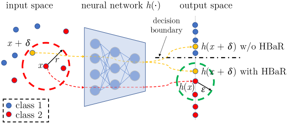
Figure 1: Illustration of HBaR for adversarial robustness. A neural network trained with HBaR gives a more constrained prediction w.r.t. perturbed inputs. Thus, it is less sensitive to adversarial examples.

2 Related Work

Adversarial Attacks. Adversarial attacks often add a constrained perturbation to natural inputs with the goal of maximizing classification loss. Szegedy et al. [26] learn a perturbation via box-constrained L-BFGS that misleads the classifier but minimally distort the input. FGSM, proposed by Goodfellow et al. [9], is a one step adversarial attack perturbing the input based on the sign of the gradient of the loss. PGD [14, 18] generates adversarial examples through multi-step projected gradient descent optimization. DeepFool [19] is an iterative attack strategy, which perturbs the input towards the direction of the decision boundaries. CW [3] applies a rectifier function regularizer to generate adversarial examples near the original input. AutoAttack (AA) [6] is an ensemble of parameter-free attacks, that also deals with common issues like gradient masking [20] and fixed step sizes [18].

Adversarial Robustness. A common approach to obtaining robust models is adversarial training, i.e., training models over adversarial examples generated via the aforementioned attacks. For example, Madry et al. [18] show that training with adversarial examples generated by PGD achieves good robustness under different attacks. DeepDefense [35] penalizes the norm of adversarial perturbations. TRADES [37] minimizes the difference between the predictions of natural and adversarial examples to get a smooth decision boundary. MART [31] pays more attention to adversarial examples from misclassified natural examples and adds a KL-divergence term between natural and adversarial samples to the cross-entropy loss. We show that our proposed method HBaR can be combined with several such state-of-the-art defense methods and boost their performance.

Information Bottleneck. The information bottleneck (IB) [28, 29] expresses a tradeoff in latent representations between information useful for output prediction and information retained about the input. IB has been employed to explore the training dynamics in deep learning models [24, 23] as well as a learning objective [1, 2]. Fischer [8] proposes a conditional entropy bottleneck (CEB) based on IB and observes its robust generalization ability empirically. Closer to us, Alemi et al. [1] propose a variational information bottleneck (VIB) for supervised learning. They empirically show that training VIB on natural examples provides good generalization and adversarial robustness. We show that HBaR can be combined with various adversarial defense methods enhancing their robustness, but also outperforms VIB [1] when given access only to natural samples. Moreover, we provide theoretical guarantees on how HBaR bounds the output perturbation induced by adversarial attacks.

Mutual Information vs. HSIC. Mutual information is difficult to compute in practice. To address this, Alemi et al. [1] estimate IB via variational inference. Ma et al. [17] replaced mutual information by the Hilbert Schmidt Independence Criterion (HSIC) and named this the HSIC Bottleneck (HB). Like Ma et al. [17], we utilize HSIC to estimate IB. However, our method is different from Ma et al. [17] in several aspects. First, they use HB to train the neural network stage-wise, layer-by-layer, without backpropagation, while we use HSIC bottleneck as a regularization in addition to cross-entropy and optimize the parameters jointly by backpropagation. Second, they only evaluate the model performance on classification accuracy, while we demonstrate adversarial robustness. Finally, we show that HBaR further enhances robustness to adversarial examples both theoretically and experimentally. Greenfeld et al. [10] use HSIC between the residual of the prediction and the input data as a learning objective for model robustness on covariate distribution shifts. Their focus is on robustness to distribution shifts, whereas our work focuses on robustness to adversarial examples, on which HBaR outperforms their proposed objective.

3 Background

3.1 Adversarial Robustness

In standard $k$-ary classification, we are given a dataset $\mathcal{D}=\{(x_{i},y_{i})\}_{i=1}^{n}$, where $x_{i}\in\mathbb{R}^{d_{X}},y_{i}\in\{0,1\}^{k}$ are i.i.d. samples drawn from joint distribution $P_{XY}$. A learner trains a neural network $h_{\theta}:\mathbb{R}^{d_{X}}\to\mathbb{R}^{k}$ parameterized by weights $\theta\in\mathbb{R}^{d_{\theta}}$ to predict $Y$ from $X$ by minimizing

$$\mathcal{L}(\theta)=\mathbb{E}_{XY}[\ell(h_{\theta}(X),Y)]\approx\frac{1}{n}\sum_{i=1}^{n}\ell(h_{\theta}(x_{i}),y_{i}),$$ (1)

where $\ell:\mathbb{R}^{k}\times\mathbb{R}^{k}\to\mathbb{R}$ is a loss function, e.g., cross-entropy. We aim to find a model $h_{\theta}$ that has high prediction accuracy but is also adversarially robust: the model should maintain high prediction accuracy against a constrained adversary, that can perturb input samples in a restricted fashion. Formally, prior to submitting a sample $x\in\mathbb{R}^{d_{X}}$ to the classifier, an adversary may perturb $x$ by an arbitrary $\delta\in\mathcal{S}_{r}$, where $\mathcal{S}_{r}\subseteq\mathbb{R}^{d_{X}}$ is the $\ell_{\infty}$-ball of radius $r$, i.e.,

$$\mathcal{S}_{r}=B(0,r)=\{\delta\in\mathbb{R}^{d_{X}}:\|\delta\|_{\infty}\leq r\}.$$ (2)

The adversarial robustness [18] of a model $h_{\theta}$ is measured by the expected loss attained by such adversarial examples, i.e.,

$$\begin{split}\mathcal{L}_{r}(\theta)=\mathbb{E}_{XY}\left[\max_{\delta\in\mathcal{S}_{r}}\ell\left(h_{\theta}(X+\delta),Y\right)\right]\approx\frac{1}{n}\sum_{i=1}^{n}\max_{\delta\in\mathcal{S}_{r}}\ell(h_{\theta}(x_{i}+\delta),y_{i}).\end{split}$$ (3)

An adversarially robust neural network $h_{\theta}$ can be obtained via adversarial training, i.e., by minimizing the adversarial robustness loss in (3) empirically over the training set $\mathcal{D}$. In practice, this amounts to training via stochastic gradient descent (SGD) over adversarial examples $x_{i}+\delta$ (see, e.g., [18]). In each epoch, $\delta$ is generated on a per sample basis via an inner optimization over $\mathcal{S}_{r}$, e.g., via projected gradient descent (PGD) on $-\mathcal{L}$.

3.2 Hilbert-Schmidt Independence Criterion (HSIC)

The Hilbert-Schmidt Independence Criterion (HSIC) is a statistical dependency measure introduced by Gretton et al. [11]. HSIC is the Hilbert-Schmidt norm of the cross-covariance operator between the distributions in Reproducing Kernel Hilbert Space (RKHS). Similar to Mutual Information (MI), HSIC captures non-linear dependencies between random variables. $\mathop{\mathrm{HSIC}}(X,Y)$ is defined as:

$$\begin{split}\mathop{\mathrm{HSIC}}(X,Y&)=\mathbb{E}_{XYX^{\prime}Y^{\prime}}\left[k_{X}\left(X,X^{\prime}\right)k_{Y^{\prime}}\left(Y,Y^{\prime}\right)\right]\\ &+\mathbb{E}_{XX^{\prime}}\left[k_{X}\left(X,X^{\prime}\right)\right]\mathbb{E}_{YY^{\prime}}\left[k_{Y}\left(Y,Y^{\prime}\right)\right]\\ &-2\mathbb{E}_{XY}\left[\mathbb{E}_{X^{\prime}}\left[k_{X}\left(X,X^{\prime}\right)\right]\mathbb{E}_{Y^{\prime}}\left[k_{Y}\left(Y,Y^{\prime}\right)\right]\right],\end{split}$$ (4)

where $X^{\prime}$, $Y^{\prime}$ are independent copies of $X$, $Y$, respectively, and $k_{X}$, $k_{Y}$ are kernels.

In practice, we often approximate HSIC empirically. Given $n$ i.i.d. samples $\{(x_{i},y_{i})\}_{i=1}^{n}$ drawn from $P_{XY}$, we estimate HSIC via:

$$\widehat{\mathop{\mathrm{HSIC}}}(X,Y)={(n-1)^{-2}}\operatorname{tr}\left(K_{X}HK_{Y}H\right),$$ (5)

where $K_{X}$ and $K_{Y}$ are kernel matrices with entries $K_{X_{ij}}=k_{X}(x_{i},x_{j})$ and $K_{Y_{ij}}=k_{Y}(y_{i},y_{j})$, respectively, and $H=\mathbf{I}-\frac{1}{n}\mathbf{1}\mathbf{1}^{\top}$ is a centering matrix.

4 Methodology

In this section, we present our method, HSIC bottleneck as regularizer (HBaR) as a means to enhance a classifier’s robustness. The effect of HBaR for adversarial robustness is illustrated in Figure 1; the HSIC bottleneck penalty reduces the sensitivity of the classifier to adversarial examples. We provide a theoretical justification for this below, in Theorems 1 and 2, but also validate the efficacy of the HSIC bottleneck extensively with experiments in Section 5.

4.1 HSIC Bottleneck as Regularizer for Robustness

Given a feedforward neural network $h_{\theta}:\mathbb{R}^{d_{X}}\to\mathbb{R}^{k}$ parameterized by $\theta$ with $M$ layers, and an input r.v. $X$, we denote by $Z_{j}\in\mathbb{R}^{d_{Z_{j}}}$, $j\in\{1,\ldots,M\}$, the output of the $j$-th layer under input $X$ (i.e., the $j$-th latent representation). We define our HBaR  learning objective as follows:

$$\begin{split}\tilde{\mathcal{L}}(\theta)=\mathcal{L}(\theta)+\lambda_{x}&\sum_{j=1}^{M}\mathop{\mathrm{HSIC}}(X,Z_{j})-\lambda_{y}\sum_{j=1}^{M}\mathop{\mathrm{HSIC}}(Y,Z_{j}),\end{split}$$ (6)

where $\mathcal{L}$ is the standard loss given by Eq. (1) and $\lambda_{x},\lambda_{y}\in\mathbb{R}_{+}$ are balancing hyperparameters.

Together, the second and third terms in Eq. (6) form the HSIC bottleneck penalty. As HSIC measures dependence between two random variables, minimizing $\mathop{\mathrm{HSIC}}(X,Z_{i})$ corresponds to removing redundant or noisy information contained in $X$. Hence, this term also naturally reduces the influence of an adversarial attack, i.e., a perturbation added on the input data. This is intuitive, but we also provide theoretical justification in the next subsection. Meanwhile, maximizing $\mathop{\mathrm{HSIC}}(Y,Z_{i})$ encourages this lack of sensitivity to the input to happen while retaining the discriminative nature of the classifier, captured by dependence to useful information w.r.t. the output label $Y$. Note that minimizing $\mathop{\mathrm{HSIC}}(X,Z_{i})$ alone would also lead to the loss of useful information, so it is necessary to keep the $\mathop{\mathrm{HSIC}}(Y,Z_{i})$ term to make sure $Z_{i}$ is informative enough of $Y$.

The overall algorithm is described in Alg. 1. In practice, we perform Stochastic Gradient Descent (SGD) over $\tilde{\mathcal{L}}$: both $\mathcal{L}$ and HSIC can be evaluated empirically over batches. For the latter, we use the estimator (5), restricted over the current batch. As we have $m$ samples in a mini-batch, the complexity of calculating the empirical HSIC (5) is $O(m^{2}d_{\bar{Z}})$ [25] for a single layer, where $d_{\bar{Z}}=\max_{j}d_{Z_{j}}$. Thus, the overall complexity for (6) is $O(Mm^{2}d_{\bar{Z}})$. This computation is highly parallelizable, thus, the additional computation time of HBaR is small when compared to training a neural network via cross-entropy only.

4.2 Combining HBaR with Adversarial Examples

HBaR can also be naturally applied in combination with adversarial training. For $r>0$ the magnitude of the perturbations introduced in adversarial examples, one can optimize the following objective instead of $\tilde{\mathcal{L}}(\theta)$ in Eq. (6):

$$\begin{split}\tilde{\mathcal{L}}_{r}(\theta)=\mathcal{L}_{r}(\theta)+\lambda_{x}\sum_{j=1}^{M}\mathop{\mathrm{HSIC}}(X,Z_{j})-\lambda_{y}\sum_{j=1}^{M}\mathop{\mathrm{HSIC}}(Y,Z_{j}),\end{split}$$ (7)

where $\mathcal{L}_{r}$ is the adversarial loss given by Eq. (3). This can be used instead of $\mathcal{L}$ in Alg. 1. Adversarial examples need to be used in the computation of the gradient of the loss $\mathcal{L}_{r}$ in each minibatch; these need to be computed on a per sample basis, e.g., via PGD over $\mathcal{S}_{r}$, at additional computational cost. Note that the natural samples $(x_{i},y_{i})$ in a batch are used to compute the HSIC bottleneck regularizer.

The HBaR penalty can similarly be combined with other adversarial learning methods and/or used with different means for selecting adversarial examples, other than PGD. We illustrate this in Section 5, where we combine HBaR with state-of-the-art adversarial learning methods TRADES [37] and MART [31].

Input: input sample tuples $\{(x_{i},y_{i})\}_{i=1}^{n}$, kernel function $k_{x},k_{y},k_{z}$, a neural network $h_{\theta}$ parameterized by $\theta$, mini-batch size $m$, learning rate $\alpha$.

Output: parameter of classifier $\theta$

while $\theta$ has not converged do

       Sample a mini-batch of size $m$ from input samples.

       Forward Propagation: calculate $z_{i}$ and $h_{\theta}(x)$.

       Compute kernel matrices for $X$, $Y$ and $Z_{i}$ using $k_{x},k_{y},k_{z}$ respectively inside mini-batch.

       Compute $\tilde{\mathcal{L}}(\theta)$ via (6), where $\mathop{\mathrm{HSIC}}$ is evaluated empirically via (5).

       Backward Propagation: $\theta\leftarrow\theta-\alpha\nabla\tilde{\mathcal{L}}(\theta)$.

end while

Algorithm 1 Robust Learning with HBaR

4.3 HBaR Robustness Guarantees

We provide here a formal justification for the use of HBaR to enhance robustness: we prove that regularization terms $\mathop{\mathrm{HSIC}}(X,Z_{j})$, $j=1,\ldots,M$ lead to classifiers which are less sensitive to input perturbations. For simplicity, we focus on the case where $k=1$ (i.e., binary classification). Let $Z\in\mathbb{R}^{d_{Z}}$ be the latent representation at some arbitrary intermediate layer of the network. That is, $Z=Z_{j}$, for some $j\in\{1,\ldots,M\}$; we omit the subscript $j$ to further reduce notation clutter. Then $h_{\theta}=(g\circ f)$, where $f:\mathbb{R}^{d_{X}}\rightarrow\mathbb{R}^{d_{Z}}$ maps the inputs to this intermediate layer, and $g:\mathbb{R}^{d_{Z}}\rightarrow\mathbb{R}$ maps the intermediate layer to the final layer. Then, $Z=f(X)$ and $g(Z)=h_{\theta}(X)\in\mathbb{R}$ are the latent and final outputs, respectively. Recall that, in HBaR, $\mathop{\mathrm{HSIC}}(X,Z)$ is associated with kernels $k_{X}$, $k_{Z}$. We make the following technical assumptions:

Assumption 1.

Let $\mathcal{X}\subseteq\mathbb{R}^{d_{X}}$, $\mathcal{Z}\subseteq\mathbb{R}^{d_{Z}}$ be the supports of random variables $X$, $Z$, respectively. We assume that both $h_{\theta}$ and $g$ are continuous and bounded functions in $\mathcal{X}$, $\mathcal{Z}$, respectively, i.e.:

$$h_{\theta}\in C(\mathcal{X}),g\in C(\mathcal{Z}).$$ (8)

Moreover, we assume that all functions $h_{\theta}$ and $g$ we consider are uniformly bounded, i.e., there exist $0<M_{\mathcal{X}},M_{\mathcal{Z}}<\infty$ such that:

$$M_{\mathcal{X}}=\max_{h_{\theta}\in C(\mathcal{X})}\|h_{\theta}\|_{\infty}\quad\text{and}\quad M_{\mathcal{Z}}=\max_{g\in C(\mathcal{Z})}\|g\|_{\infty}.$$ (9)

The continuity stated in Assumption 1 is natural, if all activation functions are continuous. Boundedness follows if, e.g., $\mathcal{X}$, $\mathcal{Z}$ are closed and bounded (i.e., compact), or if activation functions are bounded (e.g., softmax, sigmoid, etc.).

Assumption 2.

We assume kernels $k_{X}$, $k_{Z}$ are universal with respect to functions $h_{\theta}$ and $g$ that satisfy Assumption 1, i.e., if $\mathcal{F}$ and $\mathcal{G}$ are the induced RKHSs for kernels $k_{X}$ and $k_{Z}$, respectively, then for any $h_{\theta},g$ that satisfy Assumption 1 and any $\varepsilon>0$ there exist functions $h^{\prime}\in\mathcal{F}$ and $g^{\prime}\in\mathcal{G}$ such that $||h_{\theta}-h^{\prime}||_{\infty}\leq\varepsilon$ and $||g-g^{\prime}||_{\infty}\leq\varepsilon$. Moreover, functions in $\mathcal{F}$ and $\mathcal{G}$ are uniformly bounded, i.e., there exist $0<M_{\mathcal{F}},M_{\mathcal{G}}<\infty$ such that for all $h^{\prime}\in\mathcal{F}$ and all $g^{\prime}\in\mathcal{G}$:

$$M_{\mathcal{F}}=\max_{f^{\prime}\in\mathcal{F}}\|f^{\prime}\|_{\infty}\quad\text{and}\quad M_{\mathcal{G}}=\max_{g^{\prime}\in\mathcal{G}}\|g^{\prime}\|_{\infty}.$$ (10)

We note that several kernels used in practice are universal, including, e.g., the Gaussian and Laplace kernels. Moreover, given that functions that satisfy Assumption 1 are uniformly bounded by (9), such kernels can indeed remain universal while satisfying (10) via an appropriate rescaling.

Our first result shows that $\mathop{\mathrm{HSIC}}(X,Z)$ at any intermediate layer $Z$ bounds the output variance:

Theorem 1.

Under Assumptions 1 and 2, we have:

$$\operatorname{HSIC}(X,Z)\geq\frac{M_{\mathcal{F}}M_{\mathcal{G}}}{M_{\mathcal{X}}M_{\mathcal{Z}}}\sup_{\theta}\operatorname{Var}(h_{\theta}(X)).$$ (11)

The proof of Theorem 1 is in Appendix B in the supplement. We use a result by Greenfeld and Shalit [10] that links $\operatorname{HSIC}(X,Z)$ to the supremum of the covariance of bounded continuous functionals over $\mathcal{X}$ and $\mathcal{Z}$. Theorem 1 indicates that the regularizer $\mathop{\mathrm{HSIC}}(X,Z)$ at any intermediate layer naturally suppresses the variability of the output, i.e., the classifier prediction $h_{\theta}(X)$. To see this, observe that by Chebyshev’s inequality [21] the distribution of $h_{\theta}(X)$ concentrates around its mean when $\operatorname{Var}(h_{\theta}(X))$ approaches $0$. As a result, bounding $\mathop{\mathrm{HSIC}}(X,Z)$ inherently also bounds the (global) variability of the classifier (across all parameters $\theta$). This observation motivates us to also maximize $\operatorname{HSIC}(Y,Z)$ to recover essential information useful for classification: if we want to achieve good adversarial robustness as well as good predictive accuracy, we have to strike a balance between $\operatorname{HSIC}(X,Z)$ and $\operatorname{HSIC}(Y,Z)$. This perfectly aligns with the intuition behind the information bottleneck [29] and the well-known accuracy-robustness trade off [18, 37, 30, 22]. We also confirm this experimentally: we observe that both additional terms (the standard loss and $\mathop{\mathrm{HSIC}}(Y,Z)$) are necessary for ensuring good prediction performance in practice (see Table 3).

Most importantly, by further assuming that features are normal, we can show that HSIC bounds the power of an arbitrary adversary, as defined in Eq. (3):

Theorem 2.

Assume that $X\sim\mathcal{N}(0,\sigma^{2}\mathbf{I})$. Then, under Assumptions 1 and 2, we have:

$$\frac{r\sqrt{-2\log o(1)}d_{X}M_{\mathcal{Z}}}{\sigma M_{\mathcal{F}}M_{\mathcal{G}}}\operatorname{HSIC}(X,Z)+o(r)\geq\mathbb{E}[|h_{\theta}(X+\delta)-h_{\theta}(X)|],\quad\text{for all}~{}\delta\in\mathcal{S}_{r}.$$ (12)

The proof of Theorem 2 can also be found in Appendix C in the supplement. We again use the result by Greenfeld and Shalit [10] along with Stein’s Lemma [16], that relates covariances of Gaussian r.v.s and their functions to expected gradients. In particular, we apply Stein’s Lemma to the bounded functionals considered by Greenfeld and Shalit by using a truncation argument. Theorem 2 implies that $\mathop{\mathrm{HSIC}}(X,Z)$ indeed bounds the output perturbation produced by an arbitrary adversary: suppressing HSIC sufficiently can ensure that the adversary cannot alter the output significantly, in expectation. In particular, if $\operatorname{HSIC}(X,Z)=o\left(\frac{\sigma M_{\mathcal{F}}M_{\mathcal{G}}}{\sqrt{-2{\color[rgb]{0,0,0}\log o(1)}}d_{X}M_{\mathcal{Z}}}\right),$ then $\lim_{r\to 0}\sup_{\delta\in\mathcal{S}_{r}}{\mathbb{E}[|h_{\theta}(X+\delta)-h_{\theta}(X)|]}/{r}=0,$ i.e., the output is almost constant under small input perturbations.

5 Experiments

5.1 Experimental Setting

We experiment with three standard datasets, MNIST [15], CIFAR-10 [13] and CIFAR-100 [13]. We use a 4-layer LeNet [18] for MNIST, ResNet-18 [12] and WideResNet-28-10 [36] for CIFAR-10, and WideResNet-28-10 [36] for CIFAR-100. We use cross-entropy as loss $\mathcal{L}(\theta)$. Licensing information for all existing assets can be found in Appendix D in the supplement.

Algorithms. We compare HBaR to the following non-adversarial learning algorithms: Cross-Entropy (CE), Stage-Wise HSIC Bottleneck (SWHB) [17], XIC [10], and Variational Information Bottleneck (VIB) [1]. We also incorporate HBaR to several adversarial learning algorithms, as described in Section 4.2, and compare against the original methods, without the HBaR penalty. The adversarial methods we use are: Projected Gradient Descent (PGD) [18], TRADES [37], and MART [31]. Further details and parameters can be found in Appendix E in the supplement.

Performance Metrics. For all methods, we evaluate the obtained model $h_{\theta}$ via the following metrics: (a) Natural (i.e., clean test data) accuracy, and adversarial robustness via test accuracy under (b) FGSM, the fast gradient sign attack [9], (c) PGD^m, the PGD attack with $m$ steps used for the internal PGD optimization [18], (d) CW, the CW-loss within the PGD framework [4], and (e) AA, AutoAttack [6]. All five metrics are reported in percent (%) accuracy. Following prior literature, we set step size to 0.01 and radius $r=0.3$ for MNIST, and step size as $2/255$ and $r=8/255$ for CIFAR-10 and CIFAR-100. All attacks happen during the test phase and have full access to model parameters (i.e., are white-box attacks). All experiments are carried out on a Tesla V100 GPU with 32 GB memory and 5120 cores.

5.2 Results

Table 1: Natural test accuracy (in %), adversarial robustness ((in %) on FGSM, PGD, CW, and AA attacked test examples) on MNIST and CIFAR-100 of [row i, iii, v] adversarial learning baselines and [row ii, iv, vi] combining HBaR with each correspondingly. Each result is the average of five runs.

Methods	MNIST by LeNet						CIFAR-100 by WideResNet-28-10
	Natural	FGSM	PGD20	PGD40	CW	AA	Natural	FGSM	PGD10	PGD20	CW	AA
PGD	98.40	93.44	94.56	89.63	91.20	86.62	59.91	29.85	26.05	25.38	22.28	20.91
HBaR + PGD	98.66	96.02	96.44	94.35	95.10	91.57	63.84	31.59	27.90	27.21	23.23	21.61
TRADES	97.64	94.73	95.05	93.27	93.05	89.66	60.29	34.19	31.32	30.96	28.20	26.91
HBaR + TRADES	97.64	95.23	95.17	93.49	93.47	89.99	60.55	34.57	31.96	31.57	28.72	27.46
MART	98.29	95.57	95.23	93.55	93.45	88.36	58.42	32.94	29.17	28.19	27.31	25.09
HBaR + MART	98.23	96.09	96.08	94.64	94.62	89.99	58.93	33.49	30.72	30.16	28.89	25.21

Table 2: Natural test accuracy (in %), adversarial robustness ((in %) on FGSM, PGD, CW, and AA attacked test examples) on CIFAR-10 by ResNet-18 and WideResNet-28-10 of [row i, iii, v] adversarial learning baselines and [row ii, iv, vi] combining HBaR with each correspondingly. Each result is the average of five runs.

Methods	CIFAR-10 by ResNet-18						CIFAR-10 by WideResNet-28-10
	Natural	FGSM	PGD10	PGD20	CW	AA	Natural	FGSM	PGD10	PGD20	CW	AA
PGD	84.71	55.95	49.37	47.54	41.17	43.42	86.63	58.53	52.21	50.59	49.32	47.25
HBaR + PGD	85.73	57.13	49.63	48.32	41.80	44.46	87.91	59.69	52.72	51.17	49.52	47.60
TRADES	84.07	58.63	53.21	52.36	50.07	49.38	85.66	61.55	56.62	55.67	54.02	52.71
HBaR + TRADES	84.10	58.97	53.76	52.92	51.00	49.43	85.61	62.20	57.30	56.51	54.89	53.53
MART	82.15	59.85	54.75	53.67	50.12	47.97	85.94	59.39	51.30	49.46	47.94	45.48
HBaR + MART	82.44	59.86	54.84	53.89	50.53	48.21	85.52	60.54	53.42	51.81	49.32	46.99

Combining HBaR with Adversarial Examples. We show how HBaR can be used to improve robustness when used as a regularizer, as described in Section 4.2, along with state-of-the-art adversarial learning methods. We run each experiment by five times and report the mean natural test accuracy and adversarial robustness of all models on MNIST, CIFAR-10, and CIFAR-100 datasets by four architectures in Table 1 and Table 2. Combined with all adversarial training baselines, HBaR consistently improves adversarial robustness against all types of attacks on all datasets. The resulting improvements are larger than 2 standard deviations (that range between 0.05-0.2) in most cases; we report the results with standard deviations in Appendix G in the supplement. Although natural accuracy is generally restricted by the trade-off between robustness and accuracy [37], we observe that incorporating HBaR comes with an actual improvement over natural accuracy in most cases.

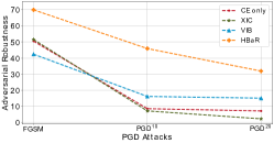
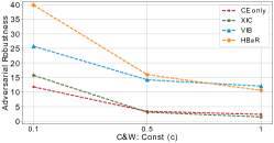
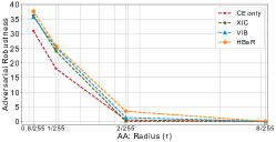
(a) PGD attacks	(b) CW attack	(c) AA using different radius

Figure 2: CIFAR-10 by ResNet-18: Adversarial robustness of IB-based baselines and proposed HBaR under (a) PGD attacks, (b) CW attack by various of constant $c$, and (c) AA using different radius. Interestingly, while achieving the highest adversarial robustness under almost all cases, HBaR achieves natural accuracy (95.27%) comparable to CE (95.32%) which is much higher than VIB (92.35%), XIC (92.93%) and SWHB (59.18%).

Adversarial Robustness Analysis without Adversarial Training. Next, we show that HBaR can achieve modest robustness even without adversarial examples during training. We evaluate the robustness of HBaR on CIFAR-10 by ResNet-18 against various adversarial attacks, and compare HBaR with other information bottleneck penalties without adversarial training in Figure 2. Specifically, we compare the robustness of HBaR with other IB-based methods under various attacks and hyperparameters. Our proposed HBaR achieves the best overall robustness against all three types of attacks while attaining competitive natural test accuracy. Interestingly, HBaR achieves natural accuracy (95.27%) comparable to CE (95.32%) which is much higher than VIB (92.35%), XIC (92.93%) and SWHB (59.18%). We observe SWHB underperforms HBaR on CIFAR-10 for both natural accuracy and robustness. One possible explanation may be that when the model is deep, minimizing HSIC without backpropagation, as in SWHB, does not suffice to transmit the learned information across layers. Compared to SWHB, HBaR backpropagates over the HSIC objective through each intermediate layer and computes gradients only once in each batch, improving accuracy and robustness while reducing computational cost significantly.

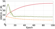
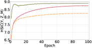
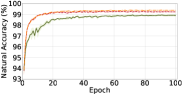
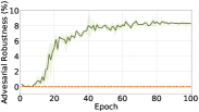
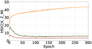
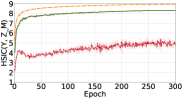
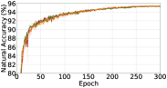
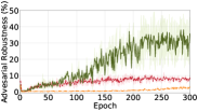
(a) HSIC$(X,Z_{M})$	(b) HSIC$(Y,Z_{M})$	(c) Natural Accuracy	(d) Adv. Robustness

Figure 3: Visualization of the HBaR quantities (a) HSIC$(X,Z_{M})$, (b) HSIC$(X,Z_{M})$, (c) natural test accuracy, and (d) adversarial robustness against PGD attack (PGD⁴⁰ and PGD²⁰ on MNIST and CIFAR-10, respectively) as a function of training epochs, on MNIST by LeNet (top) and CIFAR-10 by ResNet (bottom). Different colored lines correspond to CE, HBaR-high (HBaR with high weights $\lambda$), and HBaR-low (HBaR method small weighs $\lambda$). HBaR-low parameters are selected so that the values of the loss $\mathcal{L}$ and each of the $\mathop{\mathrm{HSIC}}$ terms are close after the first epoch.

(a) MNIST by LeNet

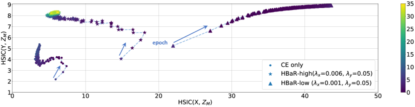
(b) CIFAR-10 by ResNet-18

Figure 4: HSIC plane dynamics versus adversarial robustness. The x-axis plots HSIC between the last intermediate layer $Z_{M}$ and the input $X$, while the y-axis plots HSIC between $Z_{M}$ and the output $Y$. The color scale indicates adversarial robustness against PGD attack (PGD⁴⁰ and PGD²⁰ on MNIST and CIFAR-10, respectively). The arrows indicate dynamic direction w.r.t. training epochs. Each marker in the figures represents a different setting: dots, stars, and triangles represent CE-only, HBaR-high, and HBaR-low, respectively, compatible with the definition in Figure 3.

Synergy between HSIC Terms. Focusing on $Z_{M}$, the last latent layer, Figure 3 shows the evolution per epoch of: (a) $\operatorname{HSIC}(X,Z_{M})$, (b) $\operatorname{HSIC}(Y,Z_{M})$, (c) natural accuracy (in %), and (d) adversarial robustness (in %) under PGD attack on MNIST and CIFAR-10. Different lines correspond to CE, HBaR-high (HBaR with high weights $\lambda$), and HBaR-low (HBaR method small weighs $\lambda$). HBaR-low parameters are selected so that the values of the loss $\mathcal{L}$ and each of the $\mathop{\mathrm{HSIC}}$ terms are close after the first epoch. Figure 3(c) illustrates that all three settings achieve good natural accuracy on both datasets. However, in Figure 3(d), only HBaR-high, that puts sufficient weight on $\mathop{\mathrm{HSIC}}$ terms, attains relatively high adversarial robustness. In Figure 3(a), we see that CE leads to high $\mathop{\mathrm{HSIC}}(X,Z_{M})$ for the shallow LeNet, but low in the (much deeper) ResNet-18, even lower than HBaR-low. Moreover, we also see that the best performer in terms of adversarial robustness, HBaR-high, lies in between the other two w.r.t. $\operatorname{HSIC}(X,Z_{M})$. Both of these observations indicate the importance of the $\operatorname{HSIC}(Y,Z_{M})$ penalty: minimizing $\operatorname{HSIC}(X,Z_{M})$ appropriately leads to good adversarial robustness, but coupling learning to labels via the third term is integral to maintaining useful label-related information in latent layers, thus resulting in good adversarial robustness. Figure 3(b) confirms this, as HBaR-high achieves relatively high $\operatorname{HSIC}(Y,Z_{M})$ on both datasets.

Figure 4 provides another perspective of the same experiments via the learning dynamics on the HSIC plane. We again observe that the best performer in terms of robustness HBaR-high lies in between the other two methods, crucially attaining a much higher $\operatorname{HSIC}(Y,Z_{M})$ than HBaR-low. Moreover, for both HBaR methods, we clearly observe the two distinct optimization phases first observed by Shwartz-Ziv and Tishby [24] in the context of the mutual information bottleneck: the fast empirical risk minimization phase, where the neural network tries to learn a meaningful representation by increasing $\operatorname{HSIC}(Y,Z_{M})$ regardless of information redundancy ($\operatorname{HSIC}(X,Z_{M})$ increasing), and the representation compression phase, where the neural network turns its focus onto compressing the latent representation by minimizing $\operatorname{HSIC}(X,Z_{M})$, while maintaining highly label-related information. Interestingly, the HBaR penalty produces the two-phase behavior even though our networks use ReLU activation functions; Shwartz et al. [24] only observed these two optimization phases on neural networks with tanh activation functions, a phenomenon further confirmed by Saxe et al. [23].

Table 3: Ablation study on HBaR. Rows [i-iv] indicate the effect of removing each component of the learning objective defined in Eq.(6) (row [v]). We evaluate each objective over $\operatorname{HSIC}(X,Z_{M})$, $\operatorname{HSIC}(Y,Z_{M})$, natural test accuracy (in %), and adversarial robustness (in %) against PGD⁴⁰ and PGD²⁰ on MNIST and CIFAR-10 respectively. We set $\lambda_{x}$ as 1 and 0.006, $\lambda_{y}$ as 50 and 0.05, for MNIST and CIFAR-10 respectively.

Rows	Objectives	MNIST by LeNet				CIFAR-10 by ResNet-18
		HSIC		Natural	PGD40	HSIC		Natural	PGD20
		$(X,Z_{M})$	$(Y,Z_{M})$			$(X,Z_{M})$	$(Y,Z_{M})$
[i]	$\mathcal{L}(\theta)$	45.29	8.73	99.23	0.00	3.45	4.76	95.32	8.57
[ii]	$\lambda_{x}\sum_{j}\operatorname{HSIC}(X,Z_{j})-\lambda_{y}\sum_{j}\operatorname{HSIC}(Y,Z_{j})$	16.45	8.65	30.08	9.47	44.37	8.72	19.30	8.58
[iii]	$\mathcal{L}(\theta)+\lambda_{x}\sum_{j}\operatorname{HSIC}(X,Z_{j})$	0.00	0.00	11.38	10.00	0.00	0.00	10.03	10.10
[iv]	$\mathcal{L}(\theta)-\lambda_{y}\sum_{j}\operatorname{HSIC}(Y,Z_{j})$	56.38	9.00	99.33	0.00	43.71	8.93	95.50	1.90
[v]	$\mathcal{L}(\theta)+\lambda_{x}\sum_{j}\operatorname{HSIC}(X,Z_{j})-\lambda_{y}\sum_{j}\operatorname{HSIC}(Y,Z_{j})$	15.68	8.89	98.90	8.33	6.07	8.30	95.35	34.85

Ablation Study. Motivated by the above observations, we turn our attention to how the three terms in the loss function in Eq. (6) affect HBaR. As illustrated in Table 3, removing any part leads to either a significant natural accuracy or robustness degradation. Specifically, using $\mathcal{L}(\theta)$ only (row [i]) lacks adversarial robustness; removing $\mathcal{L}(\theta)$ (row [ii]) or the penalty on $Y$ (row [iii]) degrades natural accuracy significantly (a similar result was also observed in [2]); finally, removing the penalty on $X$ improves the natural accuracy while degrading adversarial robustness. The three terms combined together by proper hyperparameters $\lambda_{x}$ and $\lambda_{y}$ (row [v]) achieve both high natural accuracy and adversarial robustness. We provide a comprehensive ablation study on the sensitivity of $\lambda_{x}$ and $\lambda_{y}$ and draw conclusions in Appendix F in the supplement (Tables 7 and 8).

6 Conclusions

We investigate the HSIC bottleneck as regularizer (HBaR) as a means to enhance adversarial robustness. We theoretically prove that HBaR suppresses the sensitivity of the classifier to adversarial examples while retaining its discriminative nature. One limitation of our method is that the robustness gain is modest when training with only natural examples. Moreover, a possible negative societal impact is overconfidence in adversarial robustness: over-confidence in the adversarially-robust models produced by HBaR as well as other defense methods may lead to overlooking their potential failure on newly-invented attack methods; this should be taken into account in safety-critical applications like healthcare [7] or security [27]. We extend the discussion on the limitations and potential negative societal impacts of our work in Appendix H and I, respectively, in the supplement.

7 Acknowledgements

The authors gratefully acknowledge support by the National Science Foundation under grants CCF-1937500 and CNS-2112471, and the National Institutes of Health under grant NHLBI U01HL089856.

Appendix A Checklist

1. For all authors…

   1. Do the main claims made in the abstract and introduction accurately reflect the paper’s contributions and scope? [Yes]

   2. Did you describe the limitations of your work? [Yes] See Section 6 and Appendix H in the supplement.

   3. Did you discuss any potential negative societal impacts of your work? [Yes] See Section 6 and Appendix I in the supplement.

   4. Have you read the ethics review guidelines and ensured that your paper conforms to them? [Yes]

2. If you are including theoretical results…

   1. Did you state the full set of assumptions of all theoretical results? [Yes] See Section 4.3, Assumption 1 and 2.

   2. Did you include complete proofs of all theoretical results? [Yes] See Appendix B and C in the supplement.

3. If you ran experiments…

   1. Did you include the code, data, and instructions needed to reproduce the main experimental results (either in the supplemental material or as a URL)? [Yes] See Section 5.1. We provide code and instructions to reproduce the main experimental results for our proposed method in the supplement.

   2. Did you specify all the training details (e.g., data splits, hyperparameters, how they were chosen)? [Yes] See Section 5.1 and Appendix E in the supplement.

   3. Did you report error bars (e.g., with respect to the random seed after running experiments multiple times)? [Yes] See Figure 3 in the main text and Figure 5 in the supplement.

   4. Did you include the total amount of compute and the type of resources used (e.g., type of GPUs, internal cluster, or cloud provider)? [Yes] See Section 5.1.

4. If you are using existing assets (e.g., code, data, models) or curating/releasing new assets…

   1. If your work uses existing assets, did you cite the creators? [Yes] See Section 5.1.

   2. Did you mention the license of the assets? [Yes] See Section 5.1 and Appendix D in the supplement.

   3. Did you include any new assets either in the supplemental material or as a URL? [Yes] We provide code for our proposed method in the supplement.

   4. Did you discuss whether and how consent was obtained from people whose data you’re using/curating? [N/A]

   5. Did you discuss whether the data you are using/curating contains personally identifiable information or offensive content? [N/A]

5. If you used crowdsourcing or conducted research with human subjects…

   1. Did you include the full text of instructions given to participants and screenshots, if applicable? [N/A]

   2. Did you describe any potential participant risks, with links to Institutional Review Board (IRB) approvals, if applicable? [N/A]

   3. Did you include the estimated hourly wage paid to participants and the total amount spent on participant compensation? [N/A]

Appendix B Proof of Theorem 1

Proof.

The following lemma holds:

Lemma 3.

[11, 10] Let $X$, $Z$ be random variables residing in metric spaces $\mathcal{X}$, $\mathcal{Z}$, respectively. Let also $\mathcal{F},\mathcal{G}$ be the two separable RKHSs on $\mathcal{X},\mathcal{Z}$ induced by $k_{X}$ and $k_{Z}$, respectively. Then, the following inequality holds:

$$\operatorname{HSIC}(X,Z)\geq\sup_{s\in\mathcal{F},t\in\mathcal{G}}\operatorname{Cov}[s(X),t(Z)].$$ (13)

Lemma 3 shows that HSIC bounds the supremum of the covariance between any pair of functions in the RKHS, $\mathcal{F},\mathcal{G}$. Assumption 2 states that functions in $\mathcal{F}$ and $\mathcal{G}$ are uniformly bounded by $M_{\mathcal{F}}>0$ and $M_{\mathcal{G}}>0$, respectively. Let $\mathcal{\tilde{F}}$ and $\mathcal{\tilde{G}}$ be the restriction of $\mathcal{F}$ and $\mathcal{G}$ to functions in the unit ball of the respective RKHSs through rescaling, i.e.:

$$\begin{split}\mathcal{\tilde{F}}=\left\{\frac{h}{M_{\mathcal{F}}}:h\in\mathcal{F}\right\}\quad\text{and}\quad\mathcal{\tilde{G}}=\left\{\frac{g}{M_{\mathcal{G}}}:g\in\mathcal{G}\right\}.\end{split}$$ (14)

The following lemma links the covariance of the functions in the original RKHSs to their normalized version:

Lemma 4.

[10] Suppose $\mathcal{F}$ and $\mathcal{G}$ are RKHSs over $\mathcal{X}$ and $\mathcal{Z}$, s.t. $\|s\|_{\infty}\leq M_{\mathcal{F}}$ for all $s\in\mathcal{F}$ and $\|t\|_{\infty}\leq M_{\mathcal{G}}$ for all $t\in\mathcal{G}$. Then the following holds:

$$\begin{split}\sup_{s\in\mathcal{F},t\in\mathcal{G}}\operatorname{Cov}[s(X),&t(Z)]=M_{\mathcal{F}}M_{\mathcal{G}}\sup_{s\in\tilde{\mathcal{F}},t\in\tilde{\mathcal{G}}}\operatorname{Cov}[s(X),t(Z)].\end{split}$$ (15)

For simplicity in notation, we define the following sets containing functions that satisfy Assumption 1:

$$\begin{split}C_{b}(\mathcal{X})=\left\{h\in C(\mathcal{X}):||h||_{\infty}\leq M_{\mathcal{X}}\right\}\quad\text{and}\quad C_{b}(\mathcal{Z})=\left\{g\in C(\mathcal{Z}):||g||_{\infty}\leq M_{\mathcal{Z}}\right\}.\end{split}$$ (16)

In Assumption 2, we mention that functions in $\mathcal{F}$ and $\mathcal{G}$ may require appropriate rescaling to keep the universality of corresponding kernels. To make the rescaling explicit, we define the following rescaled RKHSs:

$$\begin{split}\mathcal{\hat{F}}=\left\{\frac{M_{\mathcal{X}}}{M_{\mathcal{F}}}\cdot h:h\in\mathcal{F}\right\}\quad\text{and}\quad\mathcal{\hat{G}}=\left\{\frac{M_{\mathcal{Z}}}{M_{\mathcal{G}}}\cdot g:g\in\mathcal{G}\right\}.\end{split}$$ (17)

This rescaling ensures that $||\hat{h}||_{\infty}\leq M_{\mathcal{X}}$ for every $\hat{h}\in\mathcal{\hat{F}}$. Similarly, $||\hat{g}||_{\infty}\leq M_{\mathcal{Z}}$ for every $\hat{g}\in\mathcal{\hat{G}}$.

We also want to prove $\mathcal{F}$ is convex. Given $f,g\in\mathcal{F}$, we need to show for all $0\leq\alpha\leq 1$, the function $\alpha f+(1-\alpha)g\in\mathcal{F}$. As linear summation of RKHS functions is in the RKHS, we just need to check that $||\alpha f+(1-\alpha)g||_{\infty}\leq M_{\mathcal{F}}$; indeed:

$$||\alpha f+(1-\alpha)g||_{\infty}\leq\alpha||f||_{\infty}+(1-\alpha)||g||_{\infty}\leq\alpha M_{\mathcal{F}}+(1-\alpha)M_{\mathcal{F}}$$ (18)

We thus conclude that the bounded RKHS $\mathcal{F}$ is indeed convex. Hence any rescaling of the function, as long as it has a norm less than $M_{\mathcal{F}}$, remains inside $\mathcal{F}$.

Indeed, the following lemma holds:

Lemma 5.

If $\mathcal{F},\mathcal{G}$ are universal with respect to $C_{b}(\mathcal{X}),C_{b}(\mathcal{Z})$, then:

$$\mathcal{\hat{F}}=C_{b}(\mathcal{X})\quad\text{and}\quad\mathcal{\hat{G}}=C_{b}(\mathcal{Z}).$$ (19)

Proof.

We prove this by first showing $C_{b}(\mathcal{X})\subseteq\mathcal{\hat{F}}$ and then $\mathcal{\hat{F}}\subseteq C_{b}(\mathcal{X})$, which leads to equality of the sets.

• $C_{b}(\mathcal{X})\subseteq\mathcal{\hat{F}}$: For all $h\in C_{b}(\mathcal{X})$, we show $h\in\mathcal{\hat{F}}$. Based on the definition of $C_{b}(\mathcal{X})$ in (16), we know $\|h\|_{\infty}\leq M_{\mathcal{X}}$. From universality stated in Assumption 2, $h\in\mathcal{F}$. Let $g=\frac{M_{\mathcal{F}}}{M_{\mathcal{X}}}h$. Then $\|g\|_{\infty}=\|\frac{M_{\mathcal{F}}}{M_{\mathcal{X}}}h\|_{\infty}=\frac{M_{\mathcal{F}}}{M_{\mathcal{X}}}||h||_{\infty}\leq M_{\mathcal{F}}$. Based on the convexity of $\mathcal{F}$, $g\in\mathcal{F}$. We rescale every function in $\mathcal{F}$ by $\frac{M_{\mathcal{X}}}{M_{\mathcal{F}}}$ to form $\mathcal{\hat{F}}$, so $\frac{M_{\mathcal{X}}}{M_{\mathcal{F}}}g=\frac{M_{\mathcal{X}}}{M_{\mathcal{F}}}\frac{M_{\mathcal{F}}}{M_{\mathcal{X}}}h=h\in\mathcal{\hat{F}}$.

• $\mathcal{\hat{F}}\subseteq C_{b}(\mathcal{X})$: On the other hand, for all $h\in\mathcal{\hat{F}}$, $h$ is continuous and bounded by $M_{\mathcal{X}}$. So based on the definition of $C_{b}(\mathcal{X})$ in (16), $h\in C_{b}(\mathcal{X})$. Thus, $\mathcal{\hat{F}}\subseteq C_{b}(\mathcal{X})$.
  

Having both side of the inclusion we conclude that $\mathcal{\hat{F}}=C_{b}(\mathcal{X})$. One can prove $\mathcal{\hat{G}}=C_{b}(\mathcal{Z})$ similarly.

∎

Applying the universality of kernels from Assumption 2 we can prove the following lemma:

Lemma 6.

Let $X$, $Z$ be random variables residing in metric spaces $\mathcal{X}$, $\mathcal{Z}$ with separable RKHSs $\mathcal{F}$, $\mathcal{G}$ induced by kernel functions $k_{X}$ and $k_{Z}$, respectively, for which Assumption 2 holds. Let $\mathcal{\hat{F}}$ and $\mathcal{\hat{G}}$ be the rescaled RKHSs defined in (17). Then:

$$\frac{M_{\mathcal{X}}M_{\mathcal{Z}}}{M_{\mathcal{F}}M_{\mathcal{G}}}\sup_{s\in\mathcal{F},t\in\mathcal{G}}\operatorname{Cov}[s(X),t(Z)]=\sup_{s\in\mathcal{\hat{F}},t\in\mathcal{\hat{G}}}\operatorname{Cov}[s(X),t(Z)]=\sup_{s\in C_{b}(\mathcal{X}),t\in C_{b}(\mathcal{Z})}\operatorname{Cov}[s(X),t(Z)],$$ (20)

where $C_{b}(\mathcal{X}),C_{b}(\mathcal{Z})$ are defined in (16).

Proof.

The right equality of Lemma 6 immediately follows by Lemma 5:

$$\sup_{s\in\mathcal{\hat{F}},t\in\mathcal{\hat{G}}}\operatorname{Cov}[s(X),t(Z)]=\sup_{s\in C_{b}(\mathcal{X}),t\in C_{b}(\mathcal{Z})}\operatorname{Cov}[s(X),t(Z)].$$ (21)

Applying Lemma 4 on $\mathcal{F},\mathcal{G},\mathcal{\tilde{F}},\mathcal{\tilde{G}}$, we have:

$$\sup_{s\in\mathcal{F},t\in\mathcal{G}}\operatorname{Cov}[s(X),t(Z)]=M_{\mathcal{F}}M_{\mathcal{G}}\sup_{s\in\tilde{\mathcal{F}},t\in\tilde{\mathcal{G}}}\operatorname{Cov}[s(X),t(Z)].$$ (22)

Note that from (17) and (14), we have that the corresponding normalized space for $\mathcal{\hat{F}}$ is:

$$\begin{split}\left\{\frac{h}{M_{\mathcal{X}}}:h\in\mathcal{\hat{F}}\right\}=\left\{\frac{M_{\mathcal{X}}}{M_{\mathcal{F}}}\frac{h}{M_{\mathcal{X}}}:h\in\mathcal{{F}}\right\}=\left\{\frac{h}{M_{\mathcal{F}}}:h\in\mathcal{F}\right\}=\mathcal{\tilde{F}}.\end{split}$$ (23)

Similarly, the normalized space for $\mathcal{\hat{G}}$ is:

$$\begin{split}\left\{\frac{g}{M_{\mathcal{Z}}}:g\in\mathcal{\hat{G}}\right\}=\left\{\frac{g}{M_{\mathcal{G}}}:g\in\mathcal{G}\right\}=\mathcal{\tilde{G}}.\end{split}$$ (24)

Equation (23) implies that the normalized space induced from $\mathcal{\hat{F}}$ coincides with the normalized space induced from $\mathcal{{F}}$. Similarly, Equation (24) implies the normalized spaces for $\mathcal{G}$ and $\mathcal{\hat{G}}$ also coincide. Moreover, for all $\hat{h}\in\mathcal{\hat{F}}$, $||\hat{h}||_{\infty}\leq M_{\mathcal{X}}$ and for all $\hat{g}\in\mathcal{\hat{G}}$, $||\hat{g}||_{\infty}\leq M_{\mathcal{Z}}$. Hence, applying Lemma 4 on $\mathcal{\hat{F}},\mathcal{\hat{G}},\mathcal{\tilde{F}},\mathcal{\tilde{G}}$, we have:

$$\sup_{s\in\mathcal{\hat{F}},t\in\mathcal{\hat{G}}}\operatorname{Cov}[s(X),t(Z)]=M_{\mathcal{X}}M_{\mathcal{Z}}\sup_{s\in\tilde{\mathcal{F}},t\in\tilde{\mathcal{G}}}\operatorname{Cov}[s(X),t(Z)].$$ (25)

By dividing Equation (22) and (25), we prove the left part of Lemma 6:

$$\frac{M_{\mathcal{X}}M_{\mathcal{Z}}}{M_{\mathcal{F}}M_{\mathcal{G}}}\sup_{s\in\mathcal{F},t\in\mathcal{G}}\operatorname{Cov}[s(X),t(Z)]=\sup_{s\in\mathcal{\hat{F}},t\in\mathcal{\hat{G}}}\operatorname{Cov}[s(X),t(Z)].$$ (26)

∎

By combining Theorem 3 and Lemma 6, we have the following result:

$$\begin{split}\frac{M_{\mathcal{X}}M_{\mathcal{Z}}}{M_{\mathcal{F}}M_{\mathcal{G}}}\operatorname{HSIC}(X,Z)\geq\sup_{s\in C_{b}(\mathcal{X}),t\in C_{b}(\mathcal{Z})}\operatorname{Cov}[s(X),t(Z)].\end{split}$$ (27)

Recall that $h_{\theta}$ is a neural network from $\mathcal{X}$ to $\mathcal{Y}$, such that it can be written as composition of $g\circ f$, where $f:\mathcal{X}\to\mathcal{Z}$ and $g:\mathcal{Z}\to\mathcal{Y}$. Moreover, $h_{\theta}\in C_{b}(\mathcal{X})$ and $g\in C_{b}(\mathcal{Z})$. Using the fact that the supremum on a subset of a set is smaller or equal than the supremum on the whole set, we conclude that:

$$\begin{split}\frac{M_{\mathcal{X}}M_{\mathcal{Z}}}{M_{\mathcal{F}}M_{\mathcal{G}}}\operatorname{HSIC}(X,Z)&\geq\sup_{\theta}\operatorname{Cov}[h_{\theta}(X),g(Z))]\\ &=\sup_{\theta}\operatorname{Cov}[h_{\theta}(X),g\circ f(X)]\\ &=\sup_{\theta}\operatorname{Var}[h_{\theta}(X)].\end{split}$$ (28)

∎

Appendix C Proof of Theorem 2

Proof.

Let $t_{i}:\mathbb{R}^{d_{X}}\to\mathbb{R}$, $i=1,2,...,d_{X}$ be the following truncation functions:

$$\begin{split}t_{i}(X)=\begin{cases}-R,&\text{if}~{}X_{i}<-R,\\ X_{i},&\text{if}~{}-R\leq X_{i}\leq R,\\ R,&\text{if}~{}X_{i}>R.\end{cases}\end{split}$$ (29)

where $0<R<\infty$ and $X_{i}$ is the $i$-th dimension of $X$. Functions $t_{i}$ are continous and bounded in $\mathcal{X}$, and

$$t_{i}\in C_{b^{\prime}}(\mathcal{X}),\quad\text{where}\quad C_{b^{\prime}}(\mathcal{X})=\{t\in C(\mathcal{X}):\|t\|_{\infty}\leq R\}$$ (30)

Moreover, $g$ satisfies Assumptions 1 and 2. Similar to the proof of Theorem 1, by combining Theorem 3 and Lemma 6, we have that:

$$\begin{split}\frac{RM_{\mathcal{Z}}}{M_{\mathcal{F}}M_{\mathcal{G}}}\operatorname{HSIC}(X,Z)&\geq\sup_{t\in C_{b^{\prime}(\mathcal{X})},\ g\in C_{b}(\mathcal{Z})}\operatorname{Cov}[t(X),g(Z)]\\ &\geq\operatorname{Cov}[t_{i}(X),h_{\theta}(X)],\quad i=1,\ldots,d_{X}.\end{split}$$ (31)

Moreover, the following lemma holds:

Lemma 7.

Let $X\sim\mathcal{N}(0,\sigma^{2}\mathbf{I})$ and $t_{i}(X)$ defined by (29). For all $h_{\theta}$ that satisfy Assumption 1, we have:

$$\operatorname{Cov}[X_{i},h_{\theta}(X)]-\operatorname{Cov}[t_{i}(X),h_{\theta}(X)]\leq\frac{2M_{\mathcal{X}}\sigma}{\sqrt{2\pi}}\exp(-\frac{R^{2}}{2\sigma^{2}}),\quad\text{for all}~{}i=1,2,\ldots,d_{X}.$$ (32)

Proof.

LHS $$=\int_{-\infty}^{\infty}(x_{i}-t_{i}(x))h_{\theta}(x)\frac{1}{\sqrt{2\pi\sigma^{2}}}\exp(-\frac{x_{i}^{2}}{2\sigma^{2}})dx_{i}$$ (33a)

$$=\frac{1}{\sqrt{2\pi\sigma^{2}}}\left(\int_{-\infty}^{-R}(x_{i}+R)h_{\theta}(x)\exp(-\frac{x_{i}^{2}}{2\sigma^{2}})dx_{i}+\int_{R}^{\infty}(x_{i}-R)h_{\theta}(x)\exp(-\frac{x_{i}^{2}}{2\sigma^{2}})dx_{i}\right)$$ (33b)

$$\leq\frac{2M_{\mathcal{X}}}{\sqrt{2\pi\sigma^{2}}}\int_{R}^{\infty}(x_{i}-R)\exp(-\frac{x_{i}^{2}}{2\sigma^{2}})dx_{i}$$ (33c)

$$=\frac{2M_{\mathcal{X}}}{\sqrt{2\pi\sigma^{2}}}\int_{R}^{\infty}x_{i}\exp(-\frac{x_{i}^{2}}{2\sigma^{2}})dx_{i}-\frac{2M_{\mathcal{X}}R}{\sqrt{2\pi\sigma^{2}}}\int_{R}^{\infty}\exp(-\frac{x_{i}^{2}}{2\sigma^{2}})dx_{i}$$ (33d)

$$\leq\frac{2M_{\mathcal{X}}}{\sqrt{2\pi\sigma^{2}}}\int_{R}^{\infty}x_{i}\exp(-\frac{x_{i}^{2}}{2\sigma^{2}})dx_{i}$$ (33e)

$$=\frac{2M_{\mathcal{X}}\sigma}{\sqrt{2\pi}}\exp(-\frac{R^{2}}{2\sigma^{2}}),$$ (33f)

where (33a), (33b), (33d), (33f) are direct results from definition or simple calculation, (33c) comes from the fact that $$M_{\mathcal{X}}=\max\|h_{\theta}(X)\|_{\infty}$$ and the symmetry of two integrals, and (33e) is due to the non-negativity of the probability density function.

∎

Combining Lemma 7 with (31), we have the following result:

$$\frac{RM_{\mathcal{Z}}}{M_{\mathcal{F}}M_{\mathcal{G}}}\operatorname{HSIC}(X,Z)+\frac{2M_{\mathcal{X}}\sigma}{\sqrt{2\pi}}\exp(-\frac{R^{2}}{2\sigma^{2}})\geq\operatorname{Cov}[X_{i},h_{\theta}(X)],\quad\text{for all}~{}i=1,\ldots,d_{X}.$$ (34)

We can further bridge HSIC to adversarial robustness directly by taking advantage of the following lemma:

Lemma 8 (Stein’s Identity [16]).

Let $X=(X_{1},X_{2},\ldots X_{d_{X}})$ be multivariate normally distributed with arbitrary mean vector $\mu$ and covariance matrix $\Sigma$. For any function $h(x_{1},\ldots,x_{d_{X}})$ such that $\frac{\partial h}{\partial x_{i}}$ exists almost everywhere and $\mathbb{E}|\frac{\partial}{\partial x_{i}}|<\infty$, $i=1,\ldots,d_{X}$, we write $\nabla h(X)=(\frac{\partial h(X)}{\partial x_{1}},\ldots,\frac{\partial h(X)}{\partial x_{d_{X}}})^{\top}$. Then the following identity is true:

$$\operatorname{Cov}[X,h(X)]=\Sigma E[\nabla h(X)].$$ (35)

Specifically,

$$\operatorname{Cov}\left[X_{1},h\left(X_{1},\ldots,X_{d_{X}}\right)\right]=\sum_{i=1}^{d_{X}}\operatorname{Cov}\left(X_{1},X_{i}\right)E\left[\frac{\partial}{\partial x_{i}}h\left(X_{1},\ldots,X_{d_{X}}\right)\right]$$ (36)

Given that $X\sim\mathcal{N}(0,\sigma^{2}\mathbf{I})$, Lemma 8 implies:

$$\operatorname{Cov}\left[X_{i},h_{\theta}\left(X\right)\right]=\sigma^{2}\mathbb{E}\left[\frac{\partial}{\partial x_{i}}h_{\theta}\left(X\right)\right].$$ (37)

Combining (34) and (37), we have:

$$\frac{RM_{\mathcal{Z}}}{M_{\mathcal{F}}M_{\mathcal{G}}}\operatorname{HSIC}(X,Z)+\frac{2M_{\mathcal{X}}\sigma}{\sqrt{2\pi}}\exp(-\frac{R^{2}}{2\sigma^{2}}) \geq\sigma^{2}\mathbb{E}\left[\frac{\partial}{\partial x_{k}}h_{\theta}\left(X\right)\right].$$ (38)

Note that a similar derivation could be repeated exactly by replacing $h_{\theta}(X)$ with $-h_{\theta}(X)$. Thus, for every $i=1,2,\ldots,d_{X}$, we have:

$$\frac{RM_{\mathcal{Z}}}{M_{\mathcal{F}}M_{\mathcal{G}}}\operatorname{HSIC}(X,Z)+\frac{2M_{\mathcal{X}}\sigma}{\sqrt{2\pi}}\exp(-\frac{R^{2}}{2\sigma^{2}}) \geq\sigma^{2}\mathbb{E}\left[\left|\frac{\partial}{\partial x_{i}}h_{\theta}\left(X\right)\right|\right].$$ (39)

Summing up both sides in (39) for $i=1,2,\ldots,d_{X}$, we have:

$$\frac{d_{X}RM_{\mathcal{Z}}}{M_{\mathcal{F}}M_{\mathcal{G}}}\operatorname{HSIC}(X,Z)+\frac{2d_{X}M_{\mathcal{X}}\sigma}{\sqrt{2\pi}}\exp(-\frac{R^{2}}{2\sigma^{2}}) \geq\sigma^{2}\mathbb{E}\left[\sum_{i=1}^{d_{X}}\left|\frac{\partial}{\partial x_{i}}h_{\theta}\left(X\right)\right|\right].$$ (40)

On the other hand, for $\delta\in\mathcal{S}_{r}$, by Taylor’s theorem:

$$\mathbb{E}[|h_{\theta}(X+\delta)-h_{\theta}(X)|] \leq\mathbb{E}[|\delta^{\top}\nabla_{X}h_{\theta}(X)|]+o(r)$$ (41a)

$$\leq\mathbb{E}\left[\|\delta\|_{\infty}\|\nabla_{X}h_{\theta}(X)\|_{1}\right]+o(r)$$ (41b)

$$\leq r\mathbb{E}\left[\sum_{i=1}^{d_{X}}\left|\frac{\partial}{\partial x_{i}}h_{\theta}\left(X\right)\right|\right]+o(r),$$ (41c)

where (41b) is implied by Hölder’s inequality, and (41c) is implied by the triangle inequality.

Combining (40) and (41), we have:

$$\frac{rd_{X}RM_{\mathcal{Z}}}{\sigma^{2}M_{\mathcal{F}}M_{\mathcal{G}}}\operatorname{HSIC}(X,Z)+\frac{2rd_{X}M_{\mathcal{X}}}{\sqrt{2\pi}\sigma}\exp(-\frac{R^{2}}{2\sigma^{2}})+o(r)\geq\mathbb{E}[|h_{\theta}(X+\delta)-h_{\theta}(X)|].$$ (42)

Let $R=\sigma\sqrt{-2\log o(1)}$ where, here, $o(1)$ stands for an arbitrary function $w:\mathbb{R}\to\mathbb{R}$ s.t.

$$\lim_{r\to 0}w(r)=0.$$ (43)

Then, we have $\frac{2rd_{X}M_{\mathcal{X}}}{\sqrt{2\pi}\sigma}\exp(-\frac{R^{2}}{2\sigma^{2}})=o(r)$, because:

$$\begin{split}\lim_{r\to 0}\frac{2rd_{X}M_{\mathcal{X}}}{\sqrt{2\pi}\sigma}\exp(-\frac{R^{2}}{2\sigma^{2}})/r&=\lim_{r\to 0}\frac{2d_{X}M_{\mathcal{X}}}{\sqrt{2\pi}\sigma}\exp(\log o(1))\\ &=\lim_{r\to 0}\frac{2d_{X}M_{\mathcal{X}}}{\sqrt{2\pi}\sigma}o(1)\\ &=0\end{split}$$ (44)

Thus, we conclude that:

$$\frac{r\sqrt{-2\log o(1)}d_{X}M_{\mathcal{Z}}}{\sigma M_{\mathcal{F}}M_{\mathcal{G}}}\operatorname{HSIC}(X,Z)+o(r)\geq\mathbb{E}[|h_{\theta}(X+\delta)-h_{\theta}(X)|].$$ (45)

∎

Appendix D Licensing of Existing Assets

We provide the licensing information of each existing asset below:

Datasets.

• MNIST mnist is licensed under the Creative Commons Attribution-Share Alike 3.0 license.

• CIFAR-10 and CIFAR-100 [13] are licensed under the MIT license.

Models.

• The implementations of LeNet [18] and ResNet-18 [12] in our paper are licensed under BSD 3-Clause License.

• The implementation of WideResNet-28-10 [36] is licensed under the MIT license.

Algorithms.

• The implementations of SWHB [17], PGD [18], TRADES [37] are licensed under the MIT license.

• The implementation of VIB [1] is licensed under the Apache License 2.0.

• There are no licenses for MART [31] and XIC [10].

Adversarial Attacks. The implementations of FGSM [9], PGD [18], CW [4] and AutoAttack [6] are all licensed under the MIT license.

Appendix E Algorithm Details and Hyperparameter Tuning

Non-adversarial learning, information bottleneck based methds:

• Cross-Entropy (CE), which includes only loss $\mathcal{L}$.

• Stage-Wise HSIC Bottleneck (SWHB) [17]: This is the original HSIC bottleneck. It does not include full backpropagation over the HSIC objective: early layers are fixed stage-wise, and gradients are computed only for the current layer.

• XIC [10]: To enhance generalization over distributional shifts, this penalty includes inputs and residuals (i.e., $\mathop{\mathrm{HSIC}}(X,Y-h(X))$).

• Variational Information Bottleneck (VIB) [1]: this is a variational autoencoder that includes a mutual information bottleneck penalty.

Adversarial learning methods:

• Projected Gradient Descent (PGD) [18]: This optimizes $\mathcal{L}_{r}$, given by (3) via projected gradient ascent over $\mathcal{S}_{r}$ .

• TRADES [37]: This uses a regularization term that minimizes the difference between the predictions of natural and adversarial examples to get a smooth decision boundary.

• MART [31]: Compared to TRADES, MART pays more attention to adversarial examples from misclassified natural examples and add a KL-divergence term between natural and adversarial examples to the binary cross-entropy loss.

We use code provided by authors, including the recommended hyperparameter settings and tuning strategies. In both SWHB and HBaR, we apply Gaussian kernels for $X$ and $Z$ and a linear kernel for $Y$. For Gaussian kernels, we set $\sigma=5\sqrt{d}$, where $d$ is the dimension of the corresponding random variable.

We report all tuning parameters in Table 4. In particular, we report the parameter settings on the 4-layer LeNet [18] for MNIST, ResNet-18 [12] and WideResNet-28-10 [36] for CIFAR-10, and WideResNet-28-10 [36] for CIFAR-100 with the basic HBaR and when combining HBaR with state-of-the-art (i.e., PGD, TRADES, MART) adversarial learning.

For HBaR, to make a fair comparison with SWHB [17], we build our code, along with the implementation of PGD and PGD+HBaR, upon their framework. When combining HBaR with other state-of-the-art adversarial learning (i.e., TRADES and MART), we add our HBaR implemention to the MART framework and use recommended hyperparameter settings/tuning strategies from MART and TRADES. To make a fair comparison, we use the same network architectures among all methods with the same random weight initialization and report last epoch results.

Table 4: Parameter Summary for MNIST, CIFAR-10, and CIFAR-100. $\lambda_{x}$ and $\lambda_{y}$ are balancing hyperparameters for HBaR; $\lambda$ is balancing hyperparameter for TRADES and MART.

Dataset	param.	HBaR	PGD	PGD+HBaR	TRADES	TRADES+HBaR	MART	MART+HBaR
MNIST	$\lambda_{x}$	1	-	0.003	-	0.001	-	0.001
	$\lambda_{y}$	50	-	0.001	-	0.005	-	0.005
	$\lambda$	-			5	5	5	5
	batch size	256			256
	optimizer	adam			sgd
	learning rate	0.0001			0.01
	lr scheduler	divided by 2 at the 65-th and 90-th epoch			divided by 10 at the 20-th and 40-th epoch
	# epochs	100			50
CIFAR-10/100	$\lambda_{x}$	0.006	-	0.0005	-	0.0001	-	0.0001
	$\lambda_{y}$	0.05	-	0.005	-	0.0005	-	0.0005
	$\lambda$	-			5	5	5	5
	batch size	128			128
	optimizer	adam			sgd
	learning rate	0.01			0.01
	lr scheduler	cosine annealing			divided by 10 at the 75-th and 90-th epoch
	# epochs	300	95		95

Appendix F Sensitivity of Regularization Hyperparameters $\lambda_{x}$ and $\lambda_{y}$

We provide a comprehensive ablation study on the sensitivity of $\lambda_{x}$ and $\lambda_{y}$ on MNIST and CIFAR-10 dataset with (Table 5 and 6) and without (Table 7 and 8) adversarial training. As a conclusion, (a) we set the weight of cross-entropy loss as $1$, and empirically set $\lambda_{x}$ and $\lambda_{y}$ according to the performance on a validation set. (b) For MNIST with adversarial training, we empirically discover that $\lambda_{x}:\lambda_{y}$ ranging around $5:1$ provides better performance; for MNIST without adversarial training, $\lambda_{x}=1$ and $\lambda_{y}=50$, inspired by SWHB (Ma et al., 2020), provide the best performance. (c) for CIFAR-10 (and CIFAR-100), with and without adversarial training, $\lambda_{x}:\lambda_{y}$ ranging from $1:5$ to $1:10$ provides better performance.

Table 5: MNIST by LeNet with adversarial training: Ablation study on HBaR regularization hyperparameters $\lambda_{x}$ and $\lambda_{y}$ trained by HBaR +TRADES over the metric of natural test accuracy (%) and adversarial test robustness (PGD⁴⁰ and AA, %).

$\lambda_{x}$	$\lambda_{y}$	Natural	PGD40	AA
0.003	0.001	98.66	94.35	91.57
0.003	0	98.92	93.05	90.95
0	0.001	98.86	91.77	88.21
0.0025	0.0005	98.96	94.52	91.42
0.002	0.0005	98.92	94.13	91.33
0.0015	0.0005	98.93	94.06	91.43
0.001	0.0005	98.95	93.76	91.14
0.001	0.0002	98.92	94.61	91.37
0.0008	0.0002	98.94	94.15	91.07
0.0006	0.0002	98.91	94.13	90.72
0.0004	0.0002	98.90	93.96	90.56

Table 6: CIFAR-10 by WideResNet-28-10 with adversarial training: Ablation study on HBaR regularization hyperparameters $\lambda_{x}$ and $\lambda_{y}$ trained by HBaR +TRADES over the metric of natural test accuracy (%), and adversarial test robustness (PGD²⁰ and AA, %).

$\lambda_{x}$	$\lambda_{y}$	Natural	PGD20	AA
0.0001	0.0005	85.61	56.51	53.53
0.0001	0	80.19	49.49	45.33
0	0.0005	84.74	55.00	51.50
0.001	0.005	85.70	55.74	52.78
0.0005	0.005	84.42	55.95	52.66
0.00005	0.0005	85.37	56.43	53.40

Table 7: MNIST by LeNet without adversarial training: Ablation study on HBaR regularization hyperparameters $\lambda_{x}$ and $\lambda_{y}$ over the metric of $\operatorname{HSIC}(X,Z_{M})$, $\operatorname{HSIC}(Y,Z_{M})$, natural test accuracy (%), and adversarial test robustness (PGD⁴⁰, %).

$\lambda_{x}$	$\lambda_{y}$	HSIC		Natural	PGD40
		$(X,Z_{M})$	$(Y,Z_{M})$
CE only		45.29	8.73	99.23	0.00
0.0001	0	21.71	8.01	99.28	0.00
0.001	0	5.82	6.57	99.36	0.00
0.01	0	3.22	4.28	99.13	0.00
0	1	56.45	9.00	98.92	0.00
0.001	0.05	53.70	8.99	99.13	0.03
0.001	0.01	10.44	8.51	99.37	0.00
0.001	0.005	8.86	8.24	99.38	0.00
0.01	0.5	16.13	8.90	99.14	5.00
0.1	5	15.81	8.90	98.96	7.72
1	50	15.68	8.89	98.90	8.33
1.1	55	15.90	8.88	98.88	6.99
1.2	60	15.76	8.89	98.95	7.24
1.5	75	15.62	8.89	98.94	8.23
2	100	15.41	8.89	98.91	7.00

Table 8: CIFAR-10 by ResNet-18 without adversarial training: Ablation study on HBaR regularization hyperparameters $\lambda_{x}$ and $\lambda_{y}$ over the metric of $\operatorname{HSIC}(X,Z_{M})$, $\operatorname{HSIC}(Y,Z_{M})$, natural test accuracy (%), and adversarial test robustness (PGD²⁰, %).

$\lambda_{x}$	$\lambda_{y}$	HSIC		Natural	PGD20
		$(X,Z_{L})$	$(Y,Z_{L})$
CE only		3.45	4.76	95.32	8.57
0.001	0.05	43.48	8.93	95.36	2.91
0.002	0.05	43.15	8.92	95.55	2.29
0.003	0.05	41.95	8.90	95.51	3.98
0.004	0.05	30.12	8.77	95.45	5.23
0.005	0.05	11.56	8.45	95.44	23.73
0.006	0.05	6.07	8.30	95.35	34.85
0.007	0.05	4.81	8.24	95.13	15.80
0.008	0.05	4.44	8.21	95.13	8.43
0.009	0.05	3.96	8.14	94.70	10.83
0.01	0.05	4.09	7.87	92.33	2.90

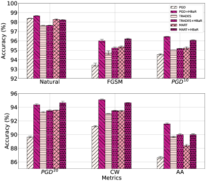
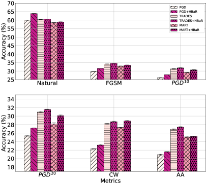
(a) MNIST by LeNet	(b) CIFAR-100 by WideResNet-28-10
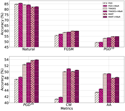
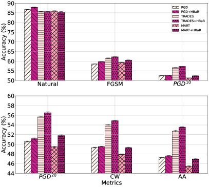
(c) CIFAR-10 by ResNet-18	(d) CIFAR-10 by WideResNet-28-10

Figure 5: Error bar of natural test accuracy (in %) and adversarial robustness ((in %) on FGSM, PGD, CW, and AA attacked test examples) on MNIST by LeNet, CIFAR-100 by WideResNet-28-10, CIFAR-10 by ResNet-18 and WideResNet-28-10 of adversarial learning baselines and combining HBaR with each correspondingly.

Table 9: MNIST by LeNet: Mean and Standard deviation of natural test accuracy (in %) and adversarial robustness ((in %) on FGSM, PGD, CW, and AA attacked test examples) of adversarial learning baselines and combining HBaR with each correspondingly.

Methods	MNIST by LeNet
	Natural	FGSM	PGD20	PGD40	CW	AA
PGD	98.40 $\pm$ 0.018	93.44 $\pm$ 0.177	94.56 $\pm$ 0.079	89.63 $\pm$ 0.117	91.20 $\pm$ 0.097	86.62 $\pm$ 0.166
HBaR + PGD	98.66 $\pm$ 0.026	96.02 $\pm$ 0.161	96.44$\pm$0.030	94.35$\pm$0.130	95.10$\pm$0.106	91.57$\pm 0.123$
TRADES	97.64$\pm$0.017	94.73$\pm$0.196	95.05$\pm$0.006	93.27$\pm$0.088	93.05$\pm$0.025	89.66$\pm$0.085
HBaR + TRADES	97.64$\pm$0.030	95.23$\pm$0.106	95.17$\pm$0.023	93.49$\pm$0.147	93.47$\pm$0.089	89.99$\pm$0.155
MART	98.29$\pm$0.059	95.57$\pm$0.113	95.23$\pm$0.144	93.55$\pm$0.018	93.45$\pm$0.077	88.36$\pm$0.179
HBaR + MART	98.23$\pm$0.054	96.09$\pm$0.074	96.08$\pm$0.035	94.64$\pm$0.125	94.62$\pm$0.06	89.99$\pm$0.13

Table 10: CIFAR-10 by ResNet-18: Mean and Standard deviation of natural test accuracy (in %) and adversarial robustness ((in %) on FGSM, PGD, CW, and AA attacked test examples) of adversarial learning baselines and combining HBaR with each correspondingly.

Methods	CIFAR-10 by ResNet-18
	Natural	FGSM	PGD10	PGD20	CW	AA
PGD	84.71$\pm$0.16	55.95$\pm$0.097	49.37$\pm$0.075	47.54$\pm$0.080	41.17$\pm$0.086	43.42$\pm$0.064
HBaR + PGD	85.73$\pm$0.166	57.13$\pm$0.099	49.63$\pm$0.058	48.32$\pm$0.103	41.80$\pm$0.116	44.46$\pm$0.169
TRADES	84.07$\pm$0.201	58.63$\pm$0.167	53.21$\pm$0.118	52.36$\pm$0.189	50.07$\pm$0.106	49.38$\pm$0.069
HBaR + TRADES	84.10$\pm$0.104	58.97$\pm$0.093	53.76$\pm$0.080	52.92$\pm$0.175	51.00$\pm$0.085	49.43$\pm$0.064
MART	82.15$\pm$0.117	59.85$\pm$0.154	54.75$\pm$0.089	53.67$\pm$0.088	50.12$\pm$0.106	47.97$\pm$0.156
HBaR + MART	82.44$\pm$0.156	59.86$\pm$0.132	54.84$\pm$0.051	53.89$\pm$0.135	50.53$\pm$0.069	48.21$\pm$0.100

Table 11: CIFAR-10 by WideResNet-28-10: Mean and Standard deviation of natural test accuracy (in %) and adversarial robustness ((in %) on FGSM, PGD, CW, and AA attacked test examples) of adversarial learning baselines and combining HBaR with each correspondingly.

Methods	CIFAR-10 by WideResNet-28-10
	Natural	FGSM	PGD10	PGD20	CW	AA
PGD	86.63$\pm$0.186	58.53$\pm$0.073	52.21$\pm$0.084	50.59$\pm$0.096	49.32$\pm$0.089	47.25$\pm$0.124
HBaR + PGD	87.91$\pm$0.102	59.69$\pm$0.097	52.72$\pm$0.081	51.17$\pm$0.152	49.52$\pm$0.174	47.60$\pm$0.131
TRADES	85.66$\pm$0.103	61.55$\pm$0.134	56.62$\pm$0.097	55.67$\pm$0.098	54.02$\pm$0.106	52.71$\pm$0.169
HBaR + TRADES	85.61$\pm$0.0133	62.20$\pm$0.102	57.30$\pm$0.059	56.51$\pm$0.136	54.89$\pm$0.098	53.53$\pm$0.127
MART	85.94$\pm$0.156	59.39$\pm$0.109	51.30$\pm$0.052	49.46$\pm$0.136	47.94$\pm$0.098	45.48$\pm$0.100
HBaR + MART	85.52$\pm$0.136	60.54$\pm$0.071	53.42$\pm$0.142	51.81$\pm$0.177	49.32$\pm$0.131	46.99$\pm$0.137

Table 12: CIFAR-100 by WideResNet-28-10: Mean and Standard deviation of natural test accuracy (in %) and adversarial robustness ((in %) on FGSM, PGD, CW, and AA attacked test examples) of adversarial learning baselines and combining HBaR with each correspondingly.

Methods	CIFAR-100 by WideResNet-28-10
	Natural	FGSM	PGD20	PGD40	CW	AA
PGD	59.91$\pm$0.116	29.85$\pm$0.117	26.05$\pm$0.106	25.38$\pm$0.129	22.28$\pm$0.079	20.91$\pm$0.133
HBaR + PGD	63.84$\pm$0.105	31.59$\pm$0.054	27.90$\pm$0.030	27.21$\pm$0.025	23.23$\pm$0.088	21.61$\pm$0.061
TRADES	60.29$\pm$0.122	34.19$\pm$0.132	31.32$\pm$0.134	30.96$\pm$0.135	28.20$\pm$0.097	26.91$\pm$0.172
HBaR + TRADES	60.55$\pm$0.065	34.57$\pm$0.068	31.96$\pm$0.067	31.57$\pm$0.079	28.72$\pm$0.071	27.46$\pm$0.098
MART	58.42$\pm$0.164	32.94$\pm$0.160	29.17$\pm$0.166	28.19$\pm$0.252	27.31$\pm$0.096	25.09$\pm$0.179
HBaR + MART	58.93$\pm$0.102	33.49$\pm$0.144	30.72$\pm$0.130	30.16$\pm$0.133	28.89$\pm$0.118	25.21$\pm$0.111

Appendix G Error Bar for Combining HBaR with Adversarial Examples

We show how HBaR can be used to improve robustness when used as a regularizer, as described in Section 4.2, along with state-of-the-art adversarial learning methods. We run each experiment by five times. Figure 5 illustrates mean and standard deviation of the natural test accuracy and adversarial robustness against various attacks on CIFAR-10 by ResNet-18 and WideResNet-28-10. Table 9, 10, 11, and 12 show the detailed standard deviation. Combined with the adversarial training baselines, HBaR consistently improves adversarial robustness against all types of attacks with small variance.

Appendix H Limitations

One limitation of our method is that the robustness gain, though beating other IB-based methods, is modest when training with only natural examples. However, the potential of getting adversarial robustness without adversarial training is interesting and worth further exploration in the future. Another limitation of our method, as well as many proposed adversarial defense methods, is the uncertain performance to new attack methods. Although we have established concrete theories and conducted comprehensive experiments, there is no guarantee that our method is able to handle novel, well-designed attacks. Finally, in our theoretical analysis in Section 4.3, we have made several assumptions for Theorem 2. While Assumptions 1 and 2 hold in practice, the distribution of input feature is not guaranteed to be standard Gaussian. Although the empirical evaluation supports the correctness of the theorem, we admit that the claim is not general enough. We aim to proof a more general version of Theorem 2 in the future, hopefully agnostic to input distributions. We will keep track of the advances in the adversarial robustness field and further improve our work correspondingly.

Appendix I Potential Societal Negative Impact

Although HBaR has great potential as a general strategy to enhance the robustness for various machine learning systems, we still need to be aware of the potential negative societal impacts it might result in. For example, over-confidence in the adversarially-robust models produced by HBaR as well as other defense methods may lead to overlooking their potential failure on newly-invented attack methods; this should be taken into account in safety-critical applications like healthcare [7] or security [27]. Another example is that, one might get insights from the theoretical analysis of our method to design stronger adversarial attacks. These attacks, if fall into the wrong hands, might cause severe societal problems. Thus, we encourage our machine learning community to further explore this field and be judicious to avoid misunderstanding or misusing of our method. Moreover, we propose to establish more reliable adversarial robustness checking routines for machine learning models deployed in safety-critical applications. For example, we should test these models with the latest adversarial attacks and make corresponding updates to them annually.

References

- [1] Alexander A Alemi, Ian Fischer, Joshua V Dillon, and Kevin Murphy. Deep variational information bottleneck. In ICLR, 2017.
- [2] Rana Ali Amjad and Bernhard C Geiger. How (not) to train your neural network using the information bottleneck principle. arXiv preprint arXiv:1802.09766, 2018.
- [3] Nicholas Carlini and David Wagner. Towards evaluating the robustness of neural networks. In 2017 ieee symposium on security and privacy (sp), pages 39–57. IEEE, 2017.
- [4] Nicholas Carlini and David A. Wagner. Towards evaluating the robustness of neural networks. In 2017 IEEE Symposium on Security and Privacy, SP 2017, San Jose, CA, USA, May 22-26, 2017, pages 39–57. IEEE Computer Society, 2017.
- [5] Alesia Chernikova, Alina Oprea, Cristina Nita-Rotaru, and BaekGyu Kim. Are self-driving cars secure? evasion attacks against deep neural networks for steering angle prediction. In 2019 IEEE Security and Privacy Workshops (SPW), pages 132–137. IEEE, 2019.
- [6] Francesco Croce and Matthias Hein. Reliable evaluation of adversarial robustness with an ensemble of diverse parameter-free attacks. In Proceedings of the 37th International Conference on Machine Learning, ICML 2020, 13-18 July 2020, Virtual Event, volume 119 of Proceedings of Machine Learning Research, pages 2206–2216, 2020.
- [7] Samuel G Finlayson, John D Bowers, Joichi Ito, Jonathan L Zittrain, Andrew L Beam, and Isaac S Kohane. Adversarial attacks on medical machine learning. Science, 363(6433):1287–1289, 2019.
- [8] Ian Fischer. The conditional entropy bottleneck. Entropy, 22(9):999, 2020.
- [9] Ian J Goodfellow, Jonathon Shlens, and Christian Szegedy. Explaining and harnessing adversarial examples. In ICLR, 2015.
- [10] Daniel Greenfeld and Uri Shalit. Robust learning with the hilbert-schmidt independence criterion. In International Conference on Machine Learning, pages 3759–3768. PMLR, 2020.
- [11] Arthur Gretton, Olivier Bousquet, Alex Smola, and Bernhard Schölkopf. Measuring statistical dependence with hilbert-schmidt norms. In International conference on algorithmic learning theory, pages 63–77. Springer, 2005.
- [12] Kaiming He, Xiangyu Zhang, Shaoqing Ren, and Jian Sun. Deep residual learning for image recognition. In CVPR, pages 770–778, 2016.
- [13] Alex Krizhevsky. Learning multiple layers of features from tiny images. Technical report, 2009.
- [14] Alexey Kurakin, Ian Goodfellow, and Samy Bengio. Adversarial machine learning at scale. In International Conference on Learning Representations, 2017.
- [15] Y. Lecun, L. Bottou, Y. Bengio, and P. Haffner. Gradient-based learning applied to document recognition. Proceedings of the IEEE, 86(11):2278–2324, 1998.
- [16] Jun S Liu. Siegel’s formula via stein’s identities. Statistics & Probability Letters, 21(3):247–251, 1994.
- [17] Wan-Duo Kurt Ma, JP Lewis, and W Bastiaan Kleijn. The hsic bottleneck: Deep learning without back-propagation. In Proceedings of the AAAI Conference on Artificial Intelligence, volume 34, pages 5085–5092, 2020.
- [18] Aleksander Madry, Aleksandar Makelov, Ludwig Schmidt, Dimitris Tsipras, and Adrian Vladu. Towards deep learning models resistant to adversarial attacks. In ICLR, 2018.
- [19] Seyed-Mohsen Moosavi-Dezfooli, Alhussein Fawzi, and Pascal Frossard. Deepfool: a simple and accurate method to fool deep neural networks. In Proceedings of the IEEE conference on computer vision and pattern recognition, pages 2574–2582, 2016.
- [20] Nicolas Papernot, Patrick McDaniel, Ian Goodfellow, Somesh Jha, Z Berkay Celik, and Ananthram Swami. Practical black-box attacks against machine learning. In Proceedings of the 2017 ACM on Asia conference on computer and communications security, pages 506–519, 2017.
- [21] Athanasios Papoulis and H Saunders. Probability, random variables and stochastic processes. 1989.
- [22] Aditi Raghunathan, Sang Michael Xie, Fanny Yang, John Duchi, and Percy Liang. Understanding and mitigating the tradeoff between robustness and accuracy. arXiv preprint arXiv:2002.10716, 2020.
- [23] Andrew M Saxe, Yamini Bansal, Joel Dapello, Madhu Advani, Artemy Kolchinsky, Brendan D Tracey, and David D Cox. On the information bottleneck theory of deep learning. Journal of Statistical Mechanics: Theory and Experiment, 2019(12):124020, 2019.
- [24] Ravid Shwartz-Ziv and Naftali Tishby. Opening the black box of deep neural networks via information. arXiv preprint arXiv:1703.00810, 2017.
- [25] Le Song, Alex Smola, Arthur Gretton, Justin Bedo, and Karsten Borgwardt. Feature selection via dependence maximization. Journal of Machine Learning Research, 13(5), 2012.
- [26] Christian Szegedy, Wojciech Zaremba, Ilya Sutskever, Joan Bruna, Dumitru Erhan, Ian Goodfellow, and Rob Fergus. Intriguing properties of neural networks. In ICLR, 2014.
- [27] Simen Thys, Wiebe Van Ranst, and Toon Goedemé. Fooling automated surveillance cameras: adversarial patches to attack person detection. In Proceedings of the IEEE/CVF Conference on Computer Vision and Pattern Recognition Workshops, pages 0–0, 2019.
- [28] Naftali Tishby, Fernando C Pereira, and William Bialek. The information bottleneck method. arXiv preprint physics/0004057, 2000.
- [29] Naftali Tishby and Noga Zaslavsky. Deep learning and the information bottleneck principle. In 2015 IEEE Information Theory Workshop (ITW), pages 1–5. IEEE, 2015.
- [30] Dimitris Tsipras, Shibani Santurkar, Logan Engstrom, Alexander Turner, and Aleksander Madry. Robustness may be at odds with accuracy. In International Conference on Learning Representations, 2019.
- [31] Yisen Wang, Difan Zou, Jinfeng Yi, James Bailey, Xingjun Ma, and Quanquan Gu. Improving adversarial robustness requires revisiting misclassified examples. In International Conference on Learning Representations, 2019.
- [32] Zifeng Wang, Batool Salehi, Andrey Gritsenko, Kaushik Chowdhury, Stratis Ioannidis, and Jennifer Dy. Open-world class discovery with kernel networks. In 2020 IEEE International Conference on Data Mining (ICDM), pages 631–640, 2020.
- [33] Chieh Wu, Zulqarnain Khan, Stratis Ioannidis, and Jennifer G Dy. Deep kernel learning for clustering. In Proceedings of the 2020 SIAM International Conference on Data Mining, pages 640–648. SIAM, 2020.
- [34] Chieh Wu, Jared Miller, Mario Sznaier, and Jennifer Dy. Solving interpretable kernel dimensionality reduction. Advances in Neural Information Processing Systems 32 (NIPS 2019), 32, 2019.
- [35] Ziang Yan, Yiwen Guo, and Changshui Zhang. Deep defense: Training dnns with improved adversarial robustness. In NeurIPS, 2018.
- [36] Sergey Zagoruyko and Nikos Komodakis. Wide residual networks. In Proceedings of the British Machine Vision Conference 2016, BMVC 2016, York, UK, September 19-22, 2016. BMVA Press, 2016.
- [37] Hongyang Zhang, Yaodong Yu, Jiantao Jiao, Eric Xing, Laurent El Ghaoui, and Michael Jordan. Theoretically principled trade-off between robustness and accuracy. In International Conference on Machine Learning, pages 7472–7482. PMLR, 2019.