Scalable semidefinite programming approach to
variational embedding for quantum many-body problems

Abstract

In quantum embedding theories, a quantum many-body system is divided into localized clusters of sites which are treated with an accurate ‘high-level’ theory and glued together self-consistently by a less accurate ‘low-level’ theory at the global scale. The recently introduced variational embedding approach for quantum many-body problems combines the insights of semidefinite relaxation and quantum embedding theory to provide a lower bound on the ground-state energy that improves as the cluster size is increased. The variational embedding method is formulated as a semidefinite program (SDP), which can suffer from poor computational scaling when treated with black-box solvers. We exploit the interpretation of this SDP as an embedding method to develop an algorithm which alternates parallelizable local updates of the high-level quantities with updates that enforce the low-level global constraints. Moreover, we show how translation invariance in lattice systems can be exploited to reduce the complexity of projecting a key matrix to the positive semidefinite cone.

1 Introduction

The problem of determining the ground state of a quantum many-body system has wide-ranging applications in physics, chemistry, and materials science. This problem can be viewed as the problem of determinining the lowest eigenvalue of a Hermitian operator on a Hilbert space whose dimension grows exponentially with the size of the system or the number of particles, such as electrons in the case of electronic structure. Here we highlight two relevant categories of approaches to taming this curse of dimensionality.

The first category is that of semidefinite relaxations, which rephrase the aforementioned energy minimization problem as an optimization problem in terms of a reduced set of physical observables, almost always a semidefinite program (SDP). In principle these observables satisfy representability constraints, i.e., constraints that ensure that they can be recovered from a bona fide quantum many-body state. However, only a subset of representability constraints can be efficiently enforced, yielding tractable optimization problems that provide lower bounds on the ground-state energy. Such approaches include the 2-RDM theories [24, 22, 4, 23, 34, 20, 1, 25, 7], as well as methods that may be classified as quantum marginal relaxations such as [19, 26, 9, 13].

Meanwhile, quantum embedding theories take the perspective of dividing a system into local clusters, small enough to be treated with a highly accurate or exact method referred to as the ‘high-level’ method. Local problems are then stitched together via a reduced set of global quantities or a less-accurate ‘low-level’ method that operates on the global scale, and the local and global perspectives are constrained to be compatible via some self-consistency condition. Such approaches include dynamical mean-field theory (DMFT) [12, 18] and density matrix embedding theory (DMET) [16, 17], as well as variants such as the energy-weighted DMET (EwDMET) [10, 11] which in a certain sense interpolates between DMFT and DMET [28].

Recently, variational embedding [21] was introduced as a semidefinite relaxation which is also a quantum embedding method. Like other relaxations such as [19, 26, 9, 13], the key optimization variables are quantum marginals for local clusters, but variational embedding additionally includes global constraints which tighten the relaxation and accommodate the treatment of, e.g., long-range interactions.

1.1 Contribution

As an SDP, variational embedding can be solved with black-box methods, as is done in [21], but scalability calls for a solver that is specially adapted to the problem. In this work, we introduce a scalable solver for this SDP which takes advantage of the embedding interpretation of the approach. The aforementioned global constraint is dualized to reduce the problem to a simpler relaxation (similar to those of [19, 26, 9, 13]) in which the global constraints have been exchanged for effective contributions to relevant Hamiltonian operators at the local scale. This problem can then be solved in a fashion in which effective problems for the key variables (the two-cluster marginals) are completely decoupled and can be solved in parallel, with dual variable optimization enforcing the self-consistency of these problems. Furthermore, translation invariance of a lattice system can be used to significantly speed up the running time.

Our approach is based on augmented Lagrangian methods (see for example [3, 29, 30]), which have been used for solving large-scale SDP problems. In particular, ADMM-type approaches can allow for sub-problems to be solved in parallel. Approaches such as [29] apply ADMM to the dual problem, whereas in [33] the primal problem is solved. Our approach differs in that the local constraints are kept in their primal form while the global positive semidefinite constraint that couples the local variables is taken into account via the introduction a dual variable. Consequently, each iteration involves the solution of many decoupled effective problems, preserving the flavor of a quantum embedding theory.

1.2 Outline

In Section 2 we provide relevant background on the ground-state eigenvalue problem, examples of interest, and the two-marginal relaxation for variational embedding introduced in [21]. (In Appendix A, additional background is provided for the context of fermionic systems.) In Section 3, we describe our optimization approach to this problem, which is an SDP. The section begins with an idealized scheme of projected gradient ascent on the dual variable to the aforementioned global constraint. In order to implement such a scheme, it is necessary to solve an effective problem in terms of the primal variables. In Section 3.1, we introduce an ADMM-type approach to this problem, and in Section 3.2 we integrate this approach with dual ascent to define our practical scheme. In Section 3.3 we explain how translation-invariance can be exploited, and in Section 3.4 we include a detailed discussion of the computational scaling. Finally in Section 4 we present numerical experiments on several model systems of quantum spins and fermions.

Acknowledgments

This work was partially supported by the National Science Foundation under Award No. 1903031 (M.L.). We thank Lin Lin for helpful discussions.

2 Preliminaries

In this section we review the formulation of variational embedding for quantum spins, following [21]. In Appendix A, we review the case of fermions (also following [21]), which requires a bit more care but nonetheless yields a semidefinite program of identical form after suitable manipulations.

2.1 The ground-state eigenvalue problem

We consider a model with $M$ sites, indexed $i=1,\ldots,M$, each endowed with a classical local state space $X_{i}$ (which shall be discrete). These in turn yields local quantum state spaces $Q_{i}=\mathbb{C}^{|X_{i}|}$. The global quantum state space (i.e., the space of wavefunctions) is then given by

$$\mathcal{Q}:=\bigotimes_{i=1}^{M}Q_{i}\simeq\mathbb{C}^{|\mathcal{X}|},$$

where $\mathcal{X}:=\prod_{i=1}^{M}X_{i}$ is the global classical state space, so quantum states (wavefunctions) correspond to complex-valued functions on the classical state space. Let $H_{i}$ (resp. $H_{ij}$) denote Hermitian operators $Q_{i}\rightarrow Q_{i}$ (resp. $Q_{ij}\rightarrow Q_{ij}$), and let $\hat{H}_{i}$ (resp. $\hat{H}_{ij}$) denote the corresponding operators $\mathcal{Q}\rightarrow\mathcal{Q}$ obtained by tensoring $H_{i}$ by the identity operator on all sites $k\neq i$ (resp. $k\neq i,j$). We consider pairwise Hamiltonian $\hat{H}:\mathcal{Q}\rightarrow\mathcal{Q}$ of the form

$$\hat{H}=\sum_{i}\hat{H}_{i}+\sum_{i<j}\hat{H}_{ij},$$

and our interest is in determining the ground-state energy, i.e., the lowest eigenvalue, of $\hat{H}$. We denote this eigenvalue by $E_{0}$, which is defined variationally by

$$E_{0}=\inf\left\{\Phi^{*}\hat{H}\Phi\,:\,\Phi\in\mathcal{Q},\>\Phi^{*}\Phi=1\right\}.$$ (2.1)

Now we review some examples of interest. First consider the case of quantum spin-$\frac{1}{2}$ systems, i.e., the case $X_{i}=\{-1,1\}$. To construct operators on $\mathcal{Q}$, one first starts with the Pauli matrices

$$\sigma^{x}=\left(\begin{array}[]{cc}0&1\\ 1&0\end{array}\right),\quad\sigma^{y}=\left(\begin{array}[]{cc}0&-i\\ i&0\end{array}\right),\quad\sigma^{z}=\left(\begin{array}[]{cc}1&0\\ 0&-1\end{array}\right),$$

which (together with the identity $I_{2}$) form a basis for the real vector space of Hermitian operators on $\mathbb{C}^{2}$. We let $\sigma_{i}^{x/y/z}$ denote the operator $\mathcal{Q}\rightarrow\mathcal{Q}$ obtained by tensoring $\sigma^{x/y/z}$ on the $i$-th site with $I_{2}$ on all other sites. Then in terms of these operators we can define the transverse-field Ising (TFI) Hamiltonian and the anti-ferromagnetic Heisenberg (AFH) Hamiltonian by

$$\hat{H}_{\mathrm{TFI}}=-h\sum_{i}\sigma_{i}^{x}-\sum_{i\sim j}\sigma_{i}^{z}\sigma_{j}^{z}$$ (2.2)

$$\hat{H}_{\mathrm{AFH}}=\sum_{i\sim j}\left[\sigma_{i}^{x}\sigma_{j}^{x}+\sigma_{i}^{y}\sigma_{j}^{y}+\sigma_{i}^{z}\sigma_{j}^{z}\right],$$ (2.3)

$h$ is a scalar paramater and summation over $i\sim j$ indicates summation over pairs of indices that are adjacent within some graph defined on the index set $\{1,\ldots,M\}$, often a rectangular lattice in some dimension. These problems have been considered as prototypical quantum many-body problems, e.g., in [5], as well as models for the study of quantum phase transitions, as in [27].

2.2 The two-marginal relaxation

In [21], the optimization problem (2.1) is reformulated as an optimization over the density operator $\rho$, which (for nondegenerate ground states) corresponds at optmality to $\Phi_{0}\Phi_{0}^{*}$ where $\Phi_{0}$ is the ground state eigenvector, i.e., the optimizer of (2.1). This optimization is in turn relaxed as a computationally tractable optimization over the quantum two-marginals

$$\rho_{ij}=\mathrm{Tr}_{\{i,j\}^{c}}[\rho],\quad i<j,$$

which are defined as partial traces of $\rho$, analogous to classical marginals. Indeed, recall [21] that for any subset $S\subset\{1,\ldots,M\}$, the partial trace $\rho_{S}=\mathrm{Tr}_{S^{c}}[\rho]$ may be defined as the unique operator on $\bigotimes_{i\in S}Q_{i}$ such that $\mathrm{Tr}[A\rho_{S}]=\mathrm{Tr}[\hat{A}\rho]$ for all operators $A$ on $\bigotimes_{i\in S}Q_{i}$ (lifted to operators $\hat{A}$ on $\mathcal{Q}$ by tensoring with the identity on $S^{c}$). In particular, $\rho_{ij}$ is an operator on $Q_{i}\otimes Q_{j}$, and moreover it is positive semidefinite with unit trace (following from the same properties for $\rho$).

Then the two-marginal relaxation of [21] reads in terms of the two marginals (and the analogously-defined one-marginals, which can be obtained from the two-marginals by further partial trace) as the following semidefinite program, whose optimal value we denote by $E_{0}^{(2)}$:

$$\underset{\{\rho_{i}\},\,\{\rho_{ij}\}_{i<j}}{\mbox{minimize}} \sum_{i}\mathrm{Tr}\left[H_{i}\rho_{i}\right]+\sum_{i<j}\mathrm{Tr}\left[H_{ij}\rho_{ij}\right]$$ (2.4)

subject to $$\rho_{ij}\succeq 0,\quad 1\leq i<j\leq M,$$ (2.8)

$$\rho_{i}=\mathrm{Tr}_{\{2\}}[\rho_{ij}],\ \rho_{j}=\mathrm{Tr}_{\{1\}}[\rho_{ij}],\quad 1\leq i<j\leq M,$$

$$\mathrm{Tr}[\rho_{i}]=1,\quad i=1,\ldots,M,$$

$$G[\{\rho_{i}\},\{\rho_{ij}\}_{i\leq j}]\succeq 0.$$

Here $G=G[\{\rho_{i}\},\{\rho_{ij}\}_{i\leq j}]$ is an operator defined linearly in terms of the one- and two-marginals, subordinate to the specification of an arbitrary collection $\{O_{i,\alpha}\,:\,\alpha=1,\ldots,n_{i}\}$ of linear operators $Q_{i}\rightarrow Q_{i}$ at each site $i=1,\ldots,M$. In specific, $G$ is specified blockwise, with blocks $G_{ij}$ for $1\leq i,j,\leq M$ of size $n_{i}\times n_{j}$ defined by

$$\left(G_{ij}\right)_{\alpha\beta}=\begin{cases}\mathrm{Tr}\left[O_{i,\alpha}^{\dagger}O_{i,\beta}\,\rho_{i}\right]&i=j\\ \mathrm{Tr}\left[\left(O_{i,\alpha}^{\dagger}\otimes O_{j,\beta}\right)\rho_{ij}\right]&i\neq j.\end{cases}$$

The choice of operators only matters up to $\mathrm{span}\{O_{i,\alpha}\,:\,\alpha=1,\ldots,n_{i}\}$, and in our numerical experiments we shall consider the complete operator collection spanning all linear maps $Q_{i}\rightarrow Q_{i}$. The last constraint (2.8) is called the global semidefinite constraint.

2.2.1 Classical marginal relaxation

To motivate the relaxation (2.4) further, we examine the problem of finding the lowest energy state of a classical energy function of a pairwise form. (This can be viewed as a special case of the more general quantum ground-state problem by taking the $H_{ij}$ to be diagonal operators.) More concretely, for $x_{i}\in X_{i},\,i=1,\ldots,M$, define an energy function

$$E(x_{1},\ldots,x_{M})=\sum_{i<j}E_{ij}(x_{i},x_{j}),$$ (2.9)

and observe that the minimizer of $E$ can be determined via the linear program

$$\underset{\mu\in\Pi(\mathcal{X})}{\arg\min}\ \sum_{(x_{1},\ldots,x_{M})\in\mathcal{X}}E(x_{1},\ldots,x_{M})\,\mu(x_{1},\ldots,x_{M}),$$ (2.10)

where $\Pi(\mathcal{X})$ is the space of probability measures on $\mathcal{X}$. Indeed, the optimizer is a $\delta$-function supported on the minimizer of $E$ (provided that it is unique). Exploiting the pairwise structure of $E$, we have

$$\underset{\{\mu_{ij}\}_{i<j}\,\mathrm{repr.}}{\arg\min}\ \sum_{i<j}\sum_{x_{i},x_{j}\in\mathcal{X}}E_{ij}(x_{i},x_{j})\,\mu_{ij}(x_{i},x_{j})$$ (2.11)

where the two-marginal variables $\{\mu_{ij}\}_{i<j}$ are constrained to be jointly representable, i.e., to be derivable as the two-marginals of a high-dimensional measure $\mu$. Enforcing this constraint demands exponential complexity, so various convex relaxation approaches have been proposed, where only certain necessary conditions for the $\{\mu_{ij}\}_{i<j}$ are kept; see, for instance, [32] for a review. In particular, the analogous convex relaxation to (2.4) is

$$\underset{\{\mu_{i}\},\,\{\mu_{ij}\}_{i<j}}{\mbox{minimize}} \sum_{i<j}\mathrm{Tr}\left[E_{ij}\mu_{ij}\right]$$ (2.12)

subject to $$\mu_{ij}\geq 0,\quad 1\leq i<j\leq M,$$ (2.16)

$$\mu_{i}=\mu_{ij}\mathbf{1},\ \mu_{j}=\mu_{ij}^{\top}\mathbf{1},\quad 1\leq i<j\leq M,$$

$$\mu_{i}^{\top}\mathbf{1}=1,\quad i=1,\ldots,M,$$

$$\begin{bmatrix}\text{diag}(\mu_{1})&\mu_{12}&\cdots&\mu_{1M}\\ \mu_{21}&&&\\ \vdots&&\ddots&\vdots\\ \mu_{M1}&\cdots&&\text{diag}(\mu_{M})\end{bmatrix}\succeq 0,$$

where $\mathbf{1}$ is an all-one vector of appropriate size. Here (2.16) and (2.16) are standard constraints for any discrete probability distributions, and (2.16) are constraints that enforces ‘local consistency’ [32] among the $\{\mu_{ij}\}_{i<j}$. The global semidefinite constraint (2.16) is discussed in [15] and [6] in the contexts of multi-marginal optimal transport and energy minimization, respectively.

2.3 Cluster relaxation

Given a quantum spin model as above and a decomposition of the sites $\{1,\ldots,M\}$ as a disjoint union $\bigcup_{i^{\prime}=1}^{M^{\prime}}C_{i^{\prime}}$ of clusters $C_{i^{\prime}}$, we may define $X_{i^{\prime}}^{\prime}:=\prod_{i\in C_{i^{\prime}}}C_{i^{\prime}}$ to be the classical state space for the $i^{\prime}$-th cluster. One see that any Hamiltonian that is pairwise with respect to sites is pairwise with respect to clusters, so by viewing our clusters as sites and applying the above formalism, we obtain a tighter relaxation [21].

2.4 Partial duality

In [21] it was shown that (2.4) admits the minimax formalization (obtained via dualization of the global semidefinite constraint (2.8))

$$E_{0}^{(2)}=\sup_{X\succeq 0}\ \mathcal{F}[X],$$ (2.17)

where

$$\mathcal{F}[X]:=\inf\left\{\sum_{i}\mathrm{Tr}\left(H_{i}[X_{ii}]\rho_{i}\right)+\sum_{i<j}\mathrm{Tr}\left(H_{ij}[X_{ij}]\rho_{ij}\right)\,:\,\{\rho_{i}\},\,\{\rho_{ij}\}_{i<j}\ \mbox{satisfy}\ \mbox{\eqref{eq:sdpC1}-\eqref{eq:sdpC3}}\right\}.$$ (2.18)

Here $X_{ij}$ denote the blocks of $X$, and the ‘effective’ Hamiltonian terms $H_{i}[X_{ii}]$ and $H_{ij}[X_{ij}]$ are defined linearly in terms of $X$ via

$$H_{i}[X_{ii}]:=H_{i}-\sum_{\alpha,\beta=1}^{n_{i}}(\overline{X}_{ii})_{\alpha\beta}O_{i,\alpha}^{\dagger}O_{i,\beta},\quad H_{ij}[X_{ij}]:=H_{i}-\left[\sum_{\alpha=1}^{n_{i}}\sum_{\beta=1}^{n_{j}}(\overline{X}_{ij})_{\alpha\beta}\left(O_{i,\alpha}^{\dagger}\otimes O_{i,\beta}\right)+\mathrm{h.c.}\right],$$ (2.19)

where ‘h.c.’ denotes the Hermitian conjugate term.

This partial dual formulation can be obtained from (2.4) by exchanging the global semidefinite constraint (2.8) for an extra term

$$-\mathrm{Tr}[X\,G[\{\rho_{i}\},\{\rho_{ij}\}_{i\leq j}]]$$

in the Lagrangian, where $X\succeq 0$ is a dual variable with respect to which the Lagrangian is to be maximized. Then (2.19) is recovered by breaking this additional term into a blockwise sum, collecting terms, and minimizing over the primal variables, subject to the remaining constraints.

Since $X$ and $G$ are dual variables [21] we have that

$$\nabla_{X}\mathcal{F}[X]=-G[\{\rho_{i}\},\{\rho_{ij}\}_{i<j}],$$ (2.20)

where $\{\rho_{i}\},\{\rho_{ij}\}_{i<j}$ are the minimizers of the infimum in (2.18).

3 Optimization approach

In order to solve the two-marginal relaxation (2.4), our point of departure is the partial dual formulation (2.17). For simplicity we consider the case in which the Hamiltonian and all variables are purely real, and we let $\Pi_{\succeq 0}$ be defined by

$$\Pi_{\succeq 0}(C):=\min_{S\succeq 0}\|S-C\|_{F}^{2},$$ (3.1)

for a symmetric matrix $A$, i.e. the Euclidean projection (in Frobenius norm) of a symmetric matrix onto the set of real symmetric positive semidefinite matrices (equivalent to setting all negative eigenvalues of the argument to zero). As an idealized scheme, we can imagine performing projected gradient ascent on (2.17), which is implemented by Algorithm 1.

Algorithm 1 Exact projected gradient ascent

1:$\varepsilon>0,\ X\succeq 0$

2:while not converged do

3:     Set $\left(\{\rho_{i}\},\{\rho_{ij}\}_{i<j}\right)$ to be the minimizer in (2.18), holding $X$ fixed

4:     $X\leftarrow\Pi_{\succeq 0}\left(X+\varepsilon G[\{\rho_{i}\},\{\rho_{ij}\}_{i<j}]\right)$

5:end while

The focus of this section is in the development of algorithm for step 3 for a general Hamiltonian, and we also study the case in the presence of translational invariance. In practice, we will not fully converge a solution to step 3 of Algorithm 1, resulting in an inexact projected gradient ascent scheme. However, in order to motivate our practical scheme, we will first discuss how to solve step 3 exactly for fixed $X$.

3.1 Details for step 2 in algorithm 1

We rephrase step 3 as the following optimization problem:

$$\underset{\{\rho_{i}\},\,\{\rho_{ij}\}_{i<j}}{\mbox{minimize}} \sum_{i}\mathrm{Tr}\left[H_{i}^{\prime}\rho_{i}\right]+\sum_{i<j}\mathrm{Tr}\left[H_{ij}^{\prime}\rho_{ij}\right]$$ (3.2)

subject to $$\rho_{ij}\succeq 0,\quad 1\leq i<j\leq M,$$

$$\rho_{i}=A_{1}[\rho_{ij}],\ \rho_{j}=A_{2}[\rho_{ij}],\quad 1\leq i<j\leq M,$$

$$\mathrm{Tr}[\rho_{i}]=1,\quad i=1,\ldots,M,$$

where $H_{i}^{\prime}:=H_{i}[X_{ii}]$, $H_{ij}^{\prime}:=H_{ij}[X_{ij}]$, and $X$ is fixed for the duration of this subsection. Moreover, for simplicity we have assumed that $m:=|X_{i}|$ is constant, and $A_{1},A_{2}$ are defined to be the linear operators $\mathrm{Tr}_{\{2\}}$ and $\mathrm{Tr}_{\{1\}}$, respectively. Hence $A_{1},A_{2}$ can be realized as sparse matrices of size $m^{2}\times m^{4}$ We then formulate an equivalent optimization problem via the introduction of dummy variables $\tilde{\rho}_{ij}$ and the inclusion of augmented Lagrangian terms in the objective:

$$\underset{\{\rho_{i}\},\,\{\rho_{ij},\tilde{\rho}_{ij}\}_{i<j}}{\mbox{minimize}} \sum_{i}\mathrm{Tr}\left[H_{i}^{\prime}\rho_{i}\right]+\sum_{i<j}\mathrm{Tr}\left[H_{ij}^{\prime}\rho_{ij}\right]$$ (3.3)

$$\quad+\ \sum_{i<j}\left(\frac{\mu}{2}\|\rho_{ij}-\tilde{\rho}_{ij}\|_{\mathrm{F}}^{2}+\frac{\nu}{2}\|\rho_{i}-A_{1}[\rho_{ij}]\|_{\mathrm{F}}^{2}+\frac{\nu}{2}\|\rho_{j}-A_{2}[\rho_{ij}]\|_{\mathrm{F}}^{2}\right)$$

subject to $$\tilde{\rho}_{ij}\succeq 0,\quad 1\leq i<j\leq M,$$

$$\Lambda_{ij}\ :\ \rho_{ij}=\tilde{\rho}_{ij},\quad 1\leq i<j\leq M,$$

$$\Lambda_{ij}^{(1)}:\ \rho_{i}=A_{1}[\rho_{ij}],\ \Lambda_{ij}^{(2)}:\ \rho_{j}=A_{2}[\rho_{ij}],\quad 1\leq i<j\leq M,$$

$$\mathrm{Tr}[\rho_{i}]=1,\quad i=1,\ldots,M,$$

where $\mu,\nu>0$ are constant parameters, and $\Lambda_{ij},\Lambda_{ij}^{(1)},\Lambda_{ij}^{(2)}\in\mathrm{End}(Q_{i}\otimes Q_{j})$ are the dual variables for the associated constraints in (3.1) and (3.1). Let $f[\{\rho_{i}\},\,\{\rho_{ij},\tilde{\rho}_{ij}\}_{i<j}]$ denote the objective function (3.3), yielding the Lagrangian

$$\mathcal{L}\left(\{\rho_{i}\},\,\{\rho_{ij},\tilde{\rho}_{ij}\}_{i<j};\,\{\Lambda_{ij},\Lambda_{ij}^{(1)},\Lambda_{ij}^{(2)}\}_{i<j}\right)$$ (3.6)

$$\ \ :=\ f[\{\rho_{i}\},\,\{\rho_{ij},\tilde{\rho}_{ij}\}_{i<j}]+\sum_{i<j}\left(\left\langle\Lambda_{ij},\tilde{\rho}_{ij}-\rho_{ij}\right\rangle_{\mathrm{F}}+\left\langle\Lambda_{ij}^{(1)},A_{1}[\rho_{ij}]-\rho_{i}\right\rangle_{\mathrm{F}}+\left\langle\Lambda_{ij}^{(2)},A_{2}[\rho_{ij}]-\rho_{j}\right\rangle_{\mathrm{F}}\right),$$

with domain specified by the (undualized) primal constraints $\tilde{\rho}_{ij}\succeq 0$ and $\mathrm{Tr}[\rho_{i}]=1$. Here $\left\langle\,\cdot\,,\,\cdot\,\right\rangle_{\mathrm{F}}$ indicates the Frobenius inner product. Then the Augmented Lagrangian method [2] for (3.2) is implemented by Algorithm 2.

Algorithm 2 Augmented Lagrangian method for (3.2)

1:$\mu,\nu>0,\ \{H^{\prime}_{i}\},\ \{H^{\prime}_{ij},\Lambda_{ij},\Lambda_{ij}^{(1)},\Lambda_{ij}^{(2)}\}_{i<j}$

2:while not converged do

3:     $\{\rho_{i}\},\{\rho_{ij},\tilde{\rho}_{ij}\}_{i<j}\leftarrow\underset{{\{\rho_{i}\},\{\rho_{ij},\tilde{\rho}_{ij}\}_{i<j}}}{\arg\min}\mathcal{L}\left(\{\rho_{i}\},\,\{\rho_{ij},\tilde{\rho}_{ij}\}_{i<j};\,\{\Lambda_{ij},\Lambda_{ij}^{(1)},\Lambda_{ij}^{(2)}\}_{i<j}\right)$

4:     for each pair $i<j$ do

5:         $\Lambda_{ij}\leftarrow\Lambda_{ij}+\mu\left(\tilde{\rho}_{ij}-\rho_{ij}\right)$

6:         $\Lambda_{ij}^{(1)}\leftarrow\Lambda_{ij}^{(1)}+\nu(A_{1}[\rho_{ij}]-\rho_{i})$

7:         $\Lambda_{ij}^{(2)}\leftarrow\Lambda_{ij}^{(2)}+\nu(A_{2}[\rho_{ij}]-\rho_{j})$

8:     end for

9:end while

In practice, it is difficult to solve step 3 of Algorithm 2 exactly. Therefore, instead of optimizing $\{\rho_{i}\},\{\rho_{ij},\tilde{\rho}_{ij}\}_{i<j}$ jointly, we consider an ADMM-type [3] substitute, namely Algorithm 3.

Algorithm 3 Pseudo-code for ADMM-type method for (3.2)

1:$\mu,\nu>0,\ \{H^{\prime}_{i},\rho_{i}\},\ \{H^{\prime}_{ij},\tilde{\rho}_{ij},\Lambda_{ij},\Lambda_{ij}^{(1)},\Lambda_{ij}^{(2)}\}_{i<j}$

2:while not converged do

3:     $\{\rho_{ij}\}_{i<j}\leftarrow\underset{{\{\rho_{ij}\}_{i<j}}}{\arg\min}\ \mathcal{L}\left(\{\rho_{i}\},\,\{\rho_{ij},\tilde{\rho}_{ij}\}_{i<j};\,\{\Lambda_{ij},\Lambda_{ij}^{(1)},\Lambda_{ij}^{(2)}\}_{i<j}\right)$

4:     $\{\rho_{i}\},\{\tilde{\rho}_{ij}\}_{i<j}\leftarrow\underset{{\{\rho_{i}\},\{\tilde{\rho}_{ij}\}_{i<j}}}{\arg\min}\mathcal{L}\left(\{\rho_{i}\},\,\{\rho_{ij},\tilde{\rho}_{ij}\}_{i<j};\,\{\Lambda_{ij},\Lambda_{ij}^{(1)},\Lambda_{ij}^{(2)}\}_{i<j}\right)$

5:     for each pair $i<j$ do

6:         $\Lambda_{ij}\leftarrow\Lambda_{ij}+\mu\left(\tilde{\rho}_{ij}-\rho_{ij}\right)$

7:         $\Lambda_{ij}^{(1)}\leftarrow\Lambda_{ij}^{(1)}+\nu(A_{1}[\rho_{ij}]-\rho_{i})$

8:         $\Lambda_{ij}^{(2)}\leftarrow\Lambda_{ij}^{(2)}+\nu(A_{2}[\rho_{ij}]-\rho_{j})$

9:     end for

10:end while

Notice that in step 3 of Algorithm 3 , the $\rho_{ij}$ are all determined independently as the solutions of decoupled optimization problems

$$\rho_{ij} \leftarrow \underset{\rho_{ij}}{\mbox{argmin}}\Bigg{\{}\left\langle H_{ij}^{\prime},\rho_{ij}\right\rangle_{\mathrm{F}}+\frac{\mu}{2}\|\rho_{ij}-\tilde{\rho}_{ij}\|_{\mathrm{F}}^{2}+\frac{\nu}{2}\|A_{1}[\rho_{ij}]-\rho_{i}\|_{\mathrm{F}}^{2}+\frac{\nu}{2}\|A_{2}[\rho_{ij}]-\rho_{j}\|_{\mathrm{F}}^{2}$$

$$\quad\quad\quad\quad\quad-\ \left\langle\Lambda_{ij},\rho_{ij}\right\rangle_{\mathrm{F}}+\left\langle\Lambda_{ij}^{(1)},A_{1}[\rho_{ij}]\right\rangle_{\mathrm{F}}+\left\langle\Lambda_{ij}^{(2)},A_{2}[\rho_{ij}]\right\rangle_{\mathrm{F}}\Bigg{\}}.$$

After suitable manipulation of the objective (neglecting constant terms), we obtain

$$\frac{1}{2}\left\langle\rho_{ij},\left(\mu+\nu A_{1}^{*}A_{1}+\nu A_{2}^{*}A_{2}\right)\rho_{ij}\right\rangle_{\mathrm{F}}-\left\langle\mu\tilde{\rho}_{ij}+A_{1}^{*}\left[\nu\rho_{i}-\Lambda_{ij}^{(1)}\right]+A_{2}^{*}\left[\nu\rho_{j}-\Lambda_{ij}^{(2)}\right]+\Lambda_{ij}-H_{ij}^{\prime},\rho_{ij}\right\rangle_{\mathrm{F}},$$

which can be exactly optimized via the update

$$\rho_{ij}\leftarrow\left(\mu+\nu A_{1}^{*}A_{1}+\nu A_{2}^{*}A_{2}\right)^{-1}\left(\mu\tilde{\rho}_{ij}+A_{1}^{*}\left[\nu\rho_{i}-\Lambda_{ij}^{(1)}\right]+A_{2}^{*}\left[\nu\rho_{j}-\Lambda_{ij}^{(2)}\right]+\Lambda_{ij}-H_{ij}^{\prime}\right).$$ (3.7)

Meanwhile, in step 4, the $\rho_{i}$ and the $\tilde{\rho}_{ij}$ can all be updated via decoupled optimization problems. In particular, we find that

$$\tilde{\rho}_{ij}\leftarrow\underset{\tilde{\rho}_{ij}\succeq 0}{\mbox{argmin}}\left\{\|\tilde{\rho}_{ij}-(\rho_{ij}-\mu^{-1}\Lambda_{ij})\|^{2}\right\}=\Pi_{\succeq 0}\left(\rho_{ij}-\mu^{-1}\Lambda_{ij}\right).$$ (3.8)

Finally we turn to the $\rho_{i}$ update. Collecting the relevant terms we have that

$$\rho_{i}\leftarrow\underset{\rho_{i}\,:\,\mathrm{Tr}[\rho_{i}]=1}{\mbox{argmin}}\left\{\left\langle H_{i}^{\prime},\rho_{i}\right\rangle_{\mathrm{F}}+\sum_{j>i}\left(\frac{\nu}{2}\|\rho_{i}-A_{1}[\rho_{ij}]\|_{\mathrm{F}}^{2}-\left\langle\Lambda_{ij}^{(1)},\rho_{i}\right\rangle_{\mathrm{F}}\right)+\sum_{j<i}\left(\frac{\nu}{2}\|\rho_{i}-A_{2}[\rho_{ji}]\|_{\mathrm{F}}^{2}-\left\langle\Lambda_{ji}^{(2)},\rho_{i}\right\rangle_{\mathrm{F}}\right)\right\}.$$

Observe that the objective may be rewritten as

$$\frac{(M-1)\nu}{2}\|\rho_{i}\|_{\mathrm{F}}^{2}-\left\langle\sum_{j>i}\left(\nu A_{1}[\rho_{ij}]+\Lambda_{ij}^{(1)}\right)+\sum_{j<i}\left(\nu A_{2}[\rho_{ji}]+\Lambda_{ji}^{(2)}\right)-H_{i}^{\prime},\rho_{i}\right\rangle_{\mathrm{F}},$$

which we must minimize subject to $\mathrm{Tr}\left[\rho_{i}\right]=1$. This is simply a constrained least squares problem, the solution of which yields the update

$$\rho_{i}\leftarrow\frac{1}{\nu(M-1)}\left(\sum_{j>i}\left(\nu A_{1}[\rho_{ij}]+\Lambda_{ij}^{(1)}\right)+\sum_{j<i}\left(\nu A_{2}[\rho_{ji}]+\Lambda_{ji}^{(2)}\right)-H_{i}^{\prime}\right)+zI_{m},$$ (3.9)

where $z$ is a Lagrange multiplier chosen to satisfy the constraint.

Then via (3.7), (3.8), and (3.9), we can rewrite Algorithm 3 concretely as the equivalent Algorithm 4. Observe that all of the for-loops in Algorithm 4 can be run in parallel.

Algorithm 4 Details of the ADMM-type method for (3.2)

1:$\mu,\nu>0,\ \{H^{\prime}_{i},\rho_{i}\},\ \{H^{\prime}_{ij},\tilde{\rho}_{ij},\Lambda_{ij},\Lambda_{ij}^{(1)},\Lambda_{ij}^{(2)}\}_{i<j}$

2:while not converged do

3:     for each pair $i<j$ do

4:         $\rho_{ij}\leftarrow\left(\mu+\nu A_{1}^{*}A_{1}+\nu A_{2}^{*}A_{2}\right)^{-1}\left(\mu\tilde{\rho}_{ij}+A_{1}^{*}\left[\nu\rho_{i}-\Lambda_{ij}^{(1)}\right]+A_{2}^{*}\left[\nu\rho_{j}-\Lambda_{ij}^{(2)}\right]+\Lambda_{ij}-H_{ij}^{\prime}\right)$

5:     end for

6:     for each pair $i<j$ do

7:         $\tilde{\rho}_{ij}\leftarrow\Pi_{\succeq 0}\left(\rho_{ij}-\mu^{-1}\Lambda_{ij}\right)$

8:     end for

9:     for each $i$ do

10:         $\rho^{\prime}_{i}\leftarrow\frac{1}{\nu(M-1)}\left(\sum_{j>i}\left(\nu A_{1}[\rho_{ij}]+\Lambda_{ij}^{(1)}\right)+\sum_{j<i}\left(\nu A_{2}[\rho_{ji}]+\Lambda_{ji}^{(2)}\right)-H_{i}^{\prime}\right)$

11:         $z\leftarrow m^{-1}(1-\mathrm{Tr}[\rho^{\prime}_{i}])$

12:         $\rho_{i}\leftarrow\rho^{\prime}_{i}+zI_{m}$

13:     end for

14:     for each pair $i<j$ do

15:         $\Lambda_{ij}\leftarrow\Lambda_{ij}+\mu\left(\tilde{\rho}_{ij}-\rho_{ij}\right)$

16:         $\Lambda_{ij}^{(1)}\leftarrow\Lambda_{ij}^{(1)}+\nu(A_{1}[\rho_{ij}]-\rho_{i})$

17:         $\Lambda_{ij}^{(2)}\leftarrow\Lambda_{ij}^{(2)}+\nu(A_{2}[\rho_{ij}]-\rho_{j})$

18:     end for

19:end while

3.2 Practical scheme

Now we return to the full Algorithm 1 where we optimize $X$ via an idealized gradient ascent. Instead of exactly implementing step 3 of Algorithm 1, we replace it with a single iteration of Algorithm 4, yielding our practical approach Algorithm 5 for solving the two-marginal relaxation (2.4).

Algorithm 5 Practical ADMM / projected dual gradient ascent method for (2.4)

1:$\varepsilon,\mu,\nu>0,\ X\succeq 0,\ \{\rho_{i}\},\ \{\tilde{\rho}_{ij},\Lambda_{ij},\Lambda_{ij}^{(1)},\Lambda_{ij}^{(2)}\}_{i<j}$

2:while not converged do

3:     for each $i$ do

4:         $H^{\prime}_{i}\leftarrow H_{i}[X_{ii}]$

5:     end for

6:     for each pair $i<j$ do

7:         $H^{\prime}_{ij}\leftarrow H_{ij}[X_{ij}]$

8:     end for

9:     for each pair $i<j$ do

10:         $\rho_{ij}\leftarrow\left(\mu+\nu A_{1}^{*}A_{1}+\nu A_{2}^{*}A_{2}\right)^{-1}\left(\mu\tilde{\rho}_{ij}+A_{1}^{*}\left[\nu\rho_{i}-\Lambda_{ij}^{(1)}\right]+A_{2}^{*}\left[\nu\rho_{j}-\Lambda_{ij}^{(2)}\right]+\Lambda_{ij}-H_{ij}^{\prime}\right)$

11:     end for

12:     for each pair $i<j$ do

13:         $\tilde{\rho}_{ij}\leftarrow\Pi_{\succeq 0}\left(\rho_{ij}-\mu^{-1}\Lambda_{ij}\right)$

14:     end for

15:     for each $i$ do

16:         $\rho^{\prime}_{i}\leftarrow\frac{1}{\nu(M-1)}\left(\sum_{j>i}\left(\nu A_{1}[\rho_{ij}]+\Lambda_{ij}^{(1)}\right)+\sum_{j<i}\left(\nu A_{2}[\rho_{ji}]+\Lambda_{ji}^{(2)}\right)-H_{i}^{\prime}\right)$

17:         $z\leftarrow m^{-1}(1-\mathrm{Tr}[\rho^{\prime}_{i}])$

18:         $\rho_{i}\leftarrow\rho^{\prime}_{i}+zI_{m}$

19:     end for

20:     for each pair $i<j$ do

21:         $\Lambda_{ij}\leftarrow\Lambda_{ij}+\mu\left(\tilde{\rho}_{ij}-\rho_{ij}\right)$

22:         $\Lambda_{ij}^{(1)}\leftarrow\Lambda_{ij}^{(1)}+\nu(A_{1}[\rho_{ij}]-\rho_{i})$

23:         $\Lambda_{ij}^{(2)}\leftarrow\Lambda_{ij}^{(2)}+\nu(A_{2}[\rho_{ij}]-\rho_{j})$

24:     end for

25:     $X\leftarrow\Pi_{\succeq 0}\left(X+\varepsilon G[\{\rho_{i}\},\{\rho_{ij}\}_{i<j}]\right)$

26:end while

3.3 Exploiting translation-invariance

One of the most expensive step in Algorithm 5 is step 24, where a projection to the positive semidefinite cone is required. We now discuss how translation-invariance of a lattice system can be exploited algorithmically in the solution of the two-marginal relaxation (2.4). It is convenient in this section to adopt zero-indexing for the site, i.e., to index the sites by the multi-index $\mathbf{i}=(i_{1},\ldots,i_{d})$ where $d$ is the lattice dimension and $i_{p}=0,\ldots,M-1$. Then we assume translation-invariance in that $\hat{H}_{\mathbf{i}}=\hat{H}_{\mathbf{0}}$ for all $i$ and $\hat{H}_{\mathbf{i}\mathbf{j}}=\hat{H}_{0,\mathbf{j}-\mathbf{i}}$ for all $i<j$. The symmetries $\rho_{\mathbf{i}}=\rho_{\mathbf{0}}$ and $\rho_{\mathbf{i}\mathbf{j}}=\rho_{0,\mathbf{j}-\mathbf{i}}$ are in turn guaranteed to be satisfied by some optimizer of (2.4) [21].

Then we can implement Algorithm 5 (whose iterations preserve this symmetry) without any reference to variables besides $\rho_{\mathbf{0}}$ and the $\rho_{\mathbf{0},\mathbf{j}}$. The main challenge is the implementation of step 25 of Algorithm 5. Given $\rho_{\mathbf{0}}$ and the $\rho_{\mathbf{0},\mathbf{j}}$, we can only compute the top row $X^{\prime}_{\mathbf{0},\mathbf{j}}$ of $X^{\prime}:=X+\varepsilon G[\{\rho_{i}\},\{\rho_{ij}\}_{i<j}]$. However, by translation invariance, the rest of $X^{\prime}$ is determined by the property that $X^{\prime}_{\mathbf{i},\mathbf{j}}=X^{\prime}_{\mathbf{0},\mathbf{j}-\mathbf{i}}$. (In the case $d=1$, $X^{\prime}$ is a block-circulant matrix, though a more general term is lacking for the case of arbitrary $d$.) Via translation invariance, $X^{\prime}$ is block-diagonalized by the block-discrete Fourier transform. More precisely, one can write $X^{\prime}$ as $X^{\prime}=(\mathcal{F}\otimes I)\hat{X}^{\prime}(\mathcal{F}^{*}\otimes I)$, where $\mathcal{F}$ indicates the appropriate $d$-dimensional discrete Fourier transform matrix, $I$ the identity matrix of the appropriate block size, $\otimes$ the Kronecker product, and $\hat{X}^{\prime}$ a block-diagonal matrix. Hence to compute the projection $\Pi_{\succeq 0}[X^{\prime}]$ we first compute the diagonal block $\hat{X}^{\prime}_{\mathbf{k}}$ of $\hat{X}^{\prime}$ as

$$\hat{X}^{\prime}_{\mathbf{k}}=\frac{1}{\sqrt{M^{d}}}\sum_{j_{1},\ldots,j_{d}=0}^{M-1}\exp\left(-\iota\frac{2\pi\mathbf{j}\cdot\mathbf{k}}{M}\right)X^{\prime}_{0,\mathbf{j}}.$$

Note that the blocks $\hat{X}^{\prime}_{\mathbf{k}}$ (concatenated into a block row) can be viewed as the entrywise discrete Fourier transform of the first block row of $X^{\prime}$, hence can be computed simultaneously via FFT. Then project $Y_{\mathbf{k}}:=\Pi_{\succeq 0}\left[\hat{X}^{\prime}_{\mathbf{k}}\right]$ for all $\mathbf{k}$, and set

$$X_{\mathbf{0},\mathbf{j}}\leftarrow\frac{1}{\sqrt{M^{d}}}\sum_{j_{1},\ldots,j_{d}=0}^{M-1}\exp\left(\iota\frac{2\pi\mathbf{j}\cdot\mathbf{k}}{M}\right)Y_{\mathbf{k}}.$$

The final pseudocode for the translation-invariant setting is given in Algorithm 6.

Algorithm 6 Translation-invariant ADMM / projected dual gradient ascent method for (2.4)

1:$\varepsilon,\mu,\nu>0,\ \left(X_{\mathbf{0},\mathbf{j}}\right),\ \rho_{\mathbf{0}},\ \{\tilde{\rho}_{\mathbf{0},\mathbf{j}},\Lambda_{\mathbf{0},\mathbf{j}},\Lambda_{\mathbf{0},\mathbf{j}}^{(1)},\Lambda_{\mathbf{0},\mathbf{j}}^{(2)}\}_{\mathbf{j}\neq\mathbf{0}}$

2:while not converged do

3:     $H^{\prime}_{\mathbf{0}}\leftarrow H_{\mathbf{0}}[X_{\mathbf{0},\mathbf{0}}]$

4:     for each $\mathbf{j}\neq\mathbf{0}$ do

5:         $H^{\prime}_{\mathbf{0},\mathbf{j}}\leftarrow H_{\mathbf{0},\mathbf{j}}[X_{\mathbf{0},\mathbf{j}}]$

6:     end for

7:     for each $\mathbf{j}\neq\mathbf{0}$ do

8:         $\rho_{\mathbf{0},\mathbf{j}}\leftarrow\left(\mu+\nu A_{1}^{*}A_{1}+\nu A_{2}^{*}A_{2}\right)^{-1}\left(\mu\tilde{\rho}_{\mathbf{0},\mathbf{j}}+A_{1}^{*}\left[\nu\rho_{\mathbf{0}}-\Lambda_{\mathbf{0},\mathbf{j}}^{(1)}\right]+A_{2}^{*}\left[\nu\rho_{\mathbf{0}}-\Lambda_{\mathbf{0},\mathbf{j}}^{(2)}\right]+\Lambda_{\mathbf{0},\mathbf{j}}-H_{\mathbf{0},\mathbf{j}}^{\prime}\right)$

9:     end for

10:     for each $\mathbf{j}\neq\mathbf{0}$ do

11:         $\tilde{\rho}_{\mathbf{0},\mathbf{j}}\leftarrow\Pi_{\succeq 0}\left(\rho_{\mathbf{0},\mathbf{j}}-\mu^{-1}\Lambda_{\mathbf{0},\mathbf{j}}\right)$

12:     end for

13:     $\rho^{\prime}_{\mathbf{0}}\leftarrow\frac{1}{\nu(M-1)}\left(\sum_{\mathbf{j}\neq\mathbf{0}}\left(\nu A_{1}[\rho_{\mathbf{0},\mathbf{j}}]+\Lambda_{\mathbf{0},\mathbf{j}}^{(1)}\right)-H_{\mathbf{0}}^{\prime}\right)$

14:     $z\leftarrow m^{-1}(1-\mathrm{Tr}[\rho^{\prime}_{\mathbf{0}}])$

15:     $\rho_{\mathbf{0}}\leftarrow\rho^{\prime}_{\mathbf{0}}+zI_{m}$

16:     for each $\mathbf{j}\neq\mathbf{0}$ do

17:         $\Lambda_{\mathbf{0},\mathbf{j}}\leftarrow\Lambda_{\mathbf{0},\mathbf{j}}+\mu\left(\tilde{\rho}_{\mathbf{0},\mathbf{j}}-\rho_{\mathbf{0},\mathbf{j}}\right)$

18:         $\Lambda_{\mathbf{0},\mathbf{j}}^{(1)}\leftarrow\Lambda_{\mathbf{0},\mathbf{j}}^{(1)}+\nu(A_{1}[\rho_{\mathbf{0},\mathbf{j}}]-\rho_{\mathbf{0}})$

19:         $\Lambda_{\mathbf{0},\mathbf{j}}^{(2)}\leftarrow\Lambda_{\mathbf{0},\mathbf{j}}^{(2)}+\nu(A_{2}[\rho_{\mathbf{0},\mathbf{j}}]-\rho_{\mathbf{0}})$

20:     end for

21:     $X_{\mathbf{0},\mathbf{0}}^{\prime}\leftarrow X_{\mathbf{0},\mathbf{0}}+\varepsilon G_{\mathbf{0},\mathbf{0}}\left[\rho_{\mathbf{0}}\right]$

22:     for each $\mathbf{j}\neq\mathbf{0}$ do

23:         $X_{\mathbf{0},\mathbf{j}}^{\prime}\leftarrow X_{\mathbf{0},\mathbf{j}}+\varepsilon G_{\mathbf{0},\mathbf{j}}\left[\rho_{\mathbf{0},\mathbf{j}}\right]$

24:     end for

25:     for each $\mathbf{k}$ do

26:         $\hat{X}^{\prime}_{\mathbf{k}}=\frac{1}{\sqrt{M^{d}}}\sum_{\mathbf{j}}\exp\left(-\iota\frac{2\pi\mathbf{j}\cdot\mathbf{k}}{M}\right)X^{\prime}_{0,\mathbf{j}}$

27:         $Y_{\mathbf{k}}\leftarrow\Pi_{\succeq 0}\left[\hat{X}^{\prime}_{\mathbf{k}}\right]$

28:     end for

29:     for each $\mathbf{j}$ do

30:         $X_{\mathbf{0},\mathbf{j}}\leftarrow\frac{1}{\sqrt{M^{d}}}\sum_{\mathbf{j}}\exp\left(\iota\frac{2\pi\mathbf{j}\cdot\mathbf{k}}{M}\right)Y_{\mathbf{k}}$

31:     end for

32:end while

3.4 Discussion of scaling

In Algorithm 5, observe that the for-loops run over $M(M-1)$ pairs $i<j$, and the scaling bottleneck among these loops is the projection $\tilde{\rho}_{ij}\leftarrow\Pi_{\succeq 0}\left(\rho_{ij}-\mu^{-1}\Lambda_{ij}\right)$ occuring in step 13. Since this step requires full diagonalization of a matrix of size $m^{2}\times m^{2}$, for which the cost is $O(m^{6})$. Meanwhile, suppose for simplicity that $n_{i}=m^{2}$, corresponding to the complete choice of operator collection $\left\{O_{\alpha,i}\,:\,\alpha=n_{i}\right\}$ for each site. Then the size of $G$ and $X$ is $Mm^{2}\times Mm^{2}$. Hence step 25, which involves a complete diagonalization of a matrix of this size, costs $O(m^{6}M^{3})$, dominating the $O(m^{6}M^{2})$ cost of the for-loops. If our sites are in fact supersites, each formed from clusters of $L$ sites in an underlying spin-$\frac{1}{2}$ model, then $m=2^{L}$. Therefore the scaling is $O(2^{6L}M^{3})$ per iteration, where $L$ is the cluster size and $M$ is the number of clusters.

Meanwhile, in the translation-invariant setting of Algorithm 6, the for-loops run only over $O(M)$ sites, so—neglecting the update for $X$—the asymptotic cost per iteration is $O(m^{6}M)$. Meanwhile, the construction of the $\hat{X}_{\mathbf{k}}^{\prime}$ in terms of the $X_{0,\mathbf{j}}$ can be achieved in time $O(m^{4}M\log M)$ via FFT. (Note that we simply treat the lattice dimension $d$ as constant.) The cost of each projection of step 27 is $O(m^{6})$ via full diagonalization, and forming the $X_{\mathbf{0},\mathbf{j}}$ in terms of the $Y_{\mathbf{k}}$ also costs $O(dm^{4}M\log M)$ in total via FFT. Hence the cost of updating $X$ (i.e., steps 21 through 30) is $O(m^{4}M\log M+m^{6}M)$. Hence the total cost per iteration of Algorithm 6, under the assumption that the sites are supersites each composed of $L$ spin-$\frac{1}{2}$ sites, is $O(2^{4L}M\log M+2^{6L}M)$, where $L$ is the cluster size and $M$ is the number of clusters.

The exponential scaling in the cluster size is unavoidable in our formulation due to the exact treatment of reduced density operators on the clusters (i.e., the cluster marginals). In this work we consider clusters of size no larger than size $L=4$. Future work will investigate the possibility of treating larger clusters by introducing further relaxation and/or compression of the optimization variables to avoid exponential scaling in the cluster size.

As a final comment, observe that every for-loop in Algorithms 5 and 6 can be run fully in parallel.

4 Numerical experiments

The numerical experiments were implemented in MATLAB following Algorithm 6. (We shall consider only translation-invariant Hamiltonians.) We present results for the transverse-field Ising (TFI) model (2.2), the anti-ferromagnetic Heisenberg (AFH) model (2.3), the spinless fermion (SF) model (A.1), and the long-range spinless fermion (LRSF) model (A.2). Note that Algorithm 6 can be applied in the fermionic case mutatis mutandi to the problem (A.3). Throughout we fix the value of the algorithmic parameters to be $\mu=\nu=10$, $\varepsilon=2$ (i.e., we do not tune them specifically to different problems). The dual variables $\{\Lambda_{ij},\Lambda_{ij}^{(1)},\Lambda_{ij}^{(2)}\}_{i\neq j}$ are all initialized to be zero, and the primal density operator variables $\{\rho_{i}\},\ \{\tilde{\rho}_{ij}\}_{i\neq j}$ are all initialized as multiples of the identity with unit trace. $X$ is initialized as the identity. We run Algorithm 6 for 10,000 iterations. (The convergence behavior will be studied in detail below.)

First we consider the TFI model on a periodic $20\times 1$ lattice, which is small enough to be solved by exact diagonalization of (2.2). We benchmark the per-site energy error of the two-marginal relaxation with clusters of size $1\times 1$, $2\times 1$, and $4\times 1$. (In these cases the semidefinite matrix variables $\rho_{ij}$ are each of size 4, 16, and 256, respectively; refer to Section 3.4 for further discussion of scaling.). The results are shown in Figure 4.1. Observe that the approximations yield lower bounds for the energy as the theory requires, and these lower bounds become tighter as the cluster size is increased. In the same figure we also consider the TFI model on a periodic $4\times 4$ lattice. Here we benchmark the energy error of the two-marginal relaxation with clusters of size $1\times 1$, $2\times 1$, and $2\times 2$.

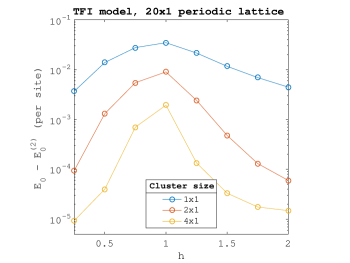
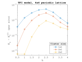
Figure 4.1: Relaxation error per site for the TFI model on $20\times 1$ and $4\times 4$ periodic lattices, pictured left and right respectively. Several cluster sizes are considered according to the legends. Note that the relaxation is exact at $h=0$ (not pictured).

We perform completely analogous experiments for the AFH model with similar conclusions. The results are shown in Tables 1 and 2.

$1\times 1$ clusters	$2\times 1$ clusters	$4\times 1$ clusters
0.5383	0.0521	0.0034

Table 1: Relaxation error per site for the AFH model on a $20\times 1$ periodic lattice for various cluster sizes.

$1\times 1$ clusters	$2\times 1$ clusters	$2\times 2$ clusters
0.6634	0.1851	0.0034

Table 2: Relaxation error per site for the AFH model on a $4\times 4$ periodic lattice for various cluster sizes.

We also benchmark the SF and LRSF models on a $20\times 1$ periodic lattice, with results pictured in Figure 4.2. Note that the fermionic relaxations are exact for $U=0$, as guaranteed in [21].

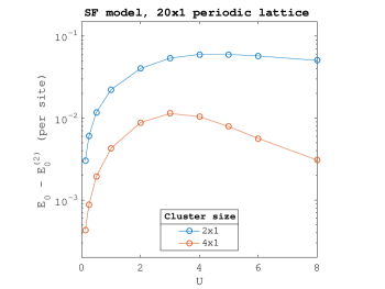
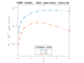
Figure 4.2: Relaxation error for the (short-range) spinless fermion (A.1) and long-range spinless fermion (A.2) models on a $20\times 1$ periodic lattice, pictured left and right respectively. Several cluster sizes are considered according to the legends. Note that the relaxation is exact at $U=0$ (not pictured).

Next we consider the TFI model on a periodic 100 × 1 lattice for $h=0.5,1,1.5$. This problem is too large to solve by exact diagonalization. We report the relaxation energy for several cluster sizes in Table 3.

	$1\times 1$ clusters	$2\times 1$ clusters	$4\times 1$ clusters
$h=0.5$	$-1.0763$	$-1.0648$	$-1.0636$
$h=1$	$-1.3084$	$-1.2829$	$-1.2761$
$h=1.5$	$-1.6835$	$-1.6724$	$-1.6720$

Table 3: Relaxation energy per site for the TFI model with $h=0.5,1,1.5$ on a $100\times 1$ periodic lattice for various cluster sizes.

We track convergence behavior of Algorithm 6 on these same problems. We use two different quantities to track convergence. The first is the per-site primal objective (i.e., energy) change between subsequent iterations. The second is the per-cluster feasibility error for the equality constraints, defined as

$$\sqrt{\frac{1}{M-1}\sum_{\mathbf{j}\neq 0}\left(\|A_{1}[\rho_{\mathbf{0},\mathbf{j}}]-\rho_{\mathbf{0}}\|_{\mathrm{F}}^{2}+\|A_{2}[\rho_{\mathbf{0},\mathbf{j}}]-\rho_{\mathbf{0}}\|_{\mathrm{F}}^{2}+\|\rho_{\mathbf{0},\mathbf{j}}-\tilde{\rho}_{\mathbf{0},\mathbf{j}}\|_{\mathrm{F}}^{2}\right)}.$$ (4.1)

We plot these quantities as functions of the iteration count in Figure 4.3. It is possible that tuning the parameters $\mu,\nu,\varepsilon$ to a specific problem and specific choice of clusters could yield smoother convergence profiles. However, even using our fixed choice for all problems, we achieve convergence of the per-site energy within $10^{-6}$ (which is dominated by the relaxation error itself) in a number of iterations that does not seem to grow with the cluster size.

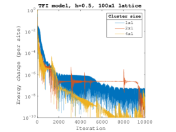
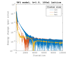
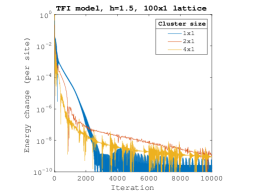
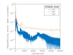
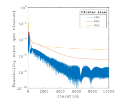
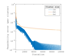
Figure 4.3: Per-site iteration-over-iteration energy change for $100\times 1$ periodic TFI model with $h=0.5,1,1.5$ and several cluster sizes (top row). Per-cluster feasibility error (4.1) for same problems (bottom row).

Then we fix clusters of size $2\times 1$ and vary the system size of the TFI model with $h=0.5,1,1.5$, to investigate the effect of system size on convergence. The results are shown in Figure 4.4. The system size does not appear to have any obvious detrimental effect on the convergence rate.

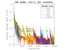
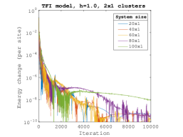
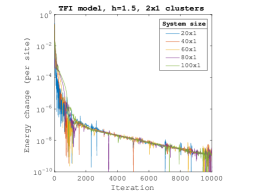
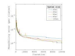
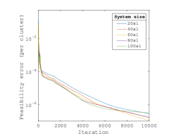
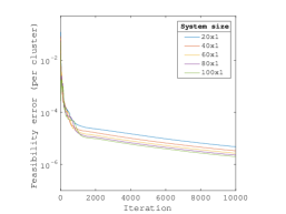
Figure 4.4: Per-site iteration-over-iteration energy change for periodic TFI models of different sizes with $h=0.5,1,1.5$ and fixed $2\times 1$ cluster size (top row). Per-cluster feasibility error (4.1) for same problems (bottom row).

To conclude, we report the relaxation energies obtained from these last experiments in Table 4. We observe that the relaxation energy approaches a limiting value in this thermodynamic limit, i.e., limit of infinite volume.

	$20\times 1$ lattice	$40\times 1$ lattice	$60\times 1$ lattice	$80\times 1$ lattice	$100\times 1$ lattice
$h=0.5$	$-1.064851$	$-1.064795$	$-1.064786$	$-1.064779$	$-1.064776$
$h=1$	$-1.283534$	$-1.283083$	$-1.283003$	$-1.282975$	$-1.282949$
$h=1.5$	$-1.672407$	$-1.672394$	$-1.672393$	$-1.672393$	$-1.672394$

Table 4: Relaxation energy per site for TFI models of several sizes with $h=0.5,1,1.5$ and clusters of fixed size $2\times 1$.

Appendix A Fermions

In this appendix we present the relevant background on fermionic many-body systems, following [21].

A.1 Background

Fermionic many-body problems in second quantization are specified in terms of the creation operators $a_{1}^{\dagger},\ldots,a_{M}^{\dagger}$ and their Hermitian adjoints, the annihilation operators $a_{i}$, which can be viewed as operators on a vector space of dimension $2^{M}$ called the Fock space $\mathcal{F}$. The key properties of these operators are the canonical anticommutation relations

$$\{a_{i},a_{j}^{\dagger}\}=\delta_{ij},\quad\{a_{i},a_{j}\}=\{a_{i}^{\dagger},a_{j}^{\dagger}\}=0,$$

where $\{\,\cdot\,,\,\cdot\,\}$ denotes the anticommutator. In terms of these operators we also define the number operators $\hat{n}_{i}:=a_{i}^{\dagger}a_{i}$, and the total number operator by $\hat{N}:=\sum_{i=1}^{M}\hat{n}_{i}$.

One can identify the Fock space with a quantum spin-$\frac{1}{2}$ state space, i.e., identify $\mathcal{F}\simeq\bigotimes^{M}\mathbb{C}^{2}\simeq\mathbb{C}^{2^{M}}$, via the correspondence

$$a_{i}^{\dagger}\rightsquigarrow\underbrace{\sigma^{z}\otimes\cdots\otimes\sigma^{z}}_{i-1\,\mathrm{factors}}\otimes\left(\begin{array}[]{cc}0&0\\ 1&0\end{array}\right)\otimes I_{2}\otimes\cdots\otimes I_{2},$$

known as the Jordan-Wigner transformation (JWT). This transformation is unnatural in the sense that it depends on the ordering of the states. More precisely, permuting the states before the JWT is not equivalent to permuting the tensor factors after the JWT. Moreover, a fermionic operator such as $a_{i}^{\dagger}a_{j}$ involving only two sites corresponds in general to a quantum spin operator involving potentially many more sites; hence the pairwise fermionic Hamiltonians that we consider below cannot be viewed in general as pairwise spin-$\frac{1}{2}$ Hamiltonians.

Next we define the notion of a pairwise fermionic Hamiltonian, and then we provide some examples. Unfortunately we cannot simply treat clusters of sites as ‘supersites’ without breaking the fermionic structure, so we approach the cluster framework directly, writing $\{1,\ldots,M\}$ as a disjoint union of clusters $\bigcup_{\gamma=1}^{N_{\mathrm{c}}}C_{\gamma}$ specified by the user. We let

$$\mathcal{A}:=\langle 1,a_{1},\ldots,a_{M},a_{1}^{\dagger},\ldots,a_{M}^{\dagger}\rangle$$

denote the star-algebra generated by the creation and annihilation operators subject to the canonical anticommutation relations $\{a_{i},a_{j}^{\dagger}\}=\delta_{ij}$, $\{a_{i},a_{j}\}=\{a_{i}^{\dagger},a_{j}^{\dagger}\}=0$, and similarly, we let

$$\mathcal{A}_{C}:=\left\langle\{1\}\cup\{a_{i},a_{i}^{\dagger}\,:\,i\in C\}\right\rangle$$

denote the subalgebra corresponding to a subset $C\subset\{1,\ldots,M\}$. Then we consider pairwise Hamiltonians $\hat{H}\in\mathcal{A}$ of the form

$$\hat{H}=\sum_{\gamma}\hat{H}_{\gamma}+\sum_{\gamma<\delta}\hat{H}_{\gamma\delta},$$

where $\hat{H}_{\gamma}\in\mathcal{A}_{C_{\gamma}}$ and $\hat{H}_{\gamma\delta}\in\mathcal{A}_{C_{\gamma}\cup C_{\delta}}$ are Hermitian operators. We are interested in the ground-state energy

$$E_{0}=\inf\left\{\langle\psi|\hat{H}|\psi\rangle\,:\,|\psi\rangle\in\mathcal{F},\,\langle\psi|\psi\rangle=1\right\}.$$

For particle-number conserving Hamiltonians (i.e., Hamiltonians that commute with $\hat{N}$), one may also consider the $N$-particle ground-state energy defined as

$$E_{0}(N)=\inf\left\{\langle\psi|\hat{H}|\psi\rangle\,:\,|\psi\rangle\in\mathcal{F},\,\langle\psi|\psi\rangle=1,\,\langle\psi|\hat{N}|\psi\rangle=N\right\},$$

though note that this is formally equivalent to the unconstrained ground-state energy $E_{0}$ after subtracting $\mu\hat{N}$ from the Hamiltonian, where the Lagrange multiplier $\mu$ is called the chemical potential.

A.2 Examples

In this work we shall consider the half-filled lattice of spinless fermions [35] specified by the Hamiltonian

$$\hat{H}=\sum_{i\sim j}\left[-a_{i}^{\dagger}a_{j}-a_{j}^{\dagger}a_{i}+U\left(\hat{n}_{i}-\frac{1}{2}\right)\left(\hat{n}_{j}-\frac{1}{2}\right)\right],$$ (A.1)

where $U$ is a scalar parameter (the ‘interaction strength’) and the notion of adjacency $i\sim j$ is defined relative to a graph (usually a rectangular lattice) on the sites $\{1,\ldots,M\}$. This operator is pairwise relative to any cluster decomposition. One can also consider an analogous model with long-range Coulomb interaction

$$\hat{H}=\sum_{i\sim j}\left[-a_{i}^{\dagger}a_{j}-a_{j}^{\dagger}a_{i}\right]+U\sum_{i\neq j}\frac{1}{d(i,j)}\left(\hat{n}_{i}-\frac{1}{2}\right)\left(\hat{n}_{j}-\frac{1}{2}\right),$$ (A.2)

where $d(i,j)$ is the Euclidean distance between sites $i$ and $j$ on the lattice.

As outlined in [21], one can also consider spinful systems such as the Hubbard model [14], as well as quantum chemistry Hamiltonians arising from electronic structure problems after a suitable choice of basis [31], e.g., the recently developed discontinuous Galerkin basis [8].

A.3 The two-marginal relaxation

In order to realize the two-marginal relaxation as a concrete semidefinite program, it is necessary to choose a JWT for each pair of clusters as follows. (Note that there will be no need to consider any global JWT.) For $1\leq\gamma\leq N_{\mathrm{c}}$, let $L_{\gamma}:=|C_{\gamma}|$, and let $\kappa_{\gamma}:C_{\gamma}\rightarrow\{1,\ldots,L_{\gamma}\}$ be a bijection specifying an ordering for the sites in the $\gamma$-th cluster. For $1\leq\gamma<\delta\leq N_{\mathrm{c}}$, let $L_{\gamma\delta}:=|C_{\gamma}|+|C_{\delta}|$, and let $\kappa_{\gamma\delta}:C_{\gamma}\cup C_{\delta}\rightarrow\{1,\ldots,L_{\gamma\delta}\}$ be the bijection specifying an ordering for the sites in the $(\gamma,\delta$)-th pair of clusters, uniquely specified by the conditions that $\kappa_{\gamma\delta}|_{C_{\gamma}}=\kappa_{\gamma}$, $\kappa_{\gamma\delta}|_{C_{\delta}}=\kappa_{\delta}$, and $\kappa_{\gamma\delta}(C_{\gamma})<\kappa_{\gamma\delta}(C_{\delta})$. These orderings fix algebra isomorphisms $\mathcal{J}_{\gamma}:\mathcal{A}_{C_{\gamma}}\rightarrow\mathrm{End}\left(\bigotimes_{i=1}^{L_{\gamma}}\mathbb{C}^{2}\right)$ and $\mathcal{J}_{\gamma\delta}:\mathcal{A}_{C_{\gamma}\cup C_{\delta}}\rightarrow\mathrm{End}\left(\bigotimes_{i=1}^{L_{\gamma\delta}}\mathbb{C}^{2}\right)$ via the appropriate JWTs. Then the two-marginal relaxation is given concretely by

$$\underset{\{\rho_{\gamma}\},\,\{\rho_{\gamma\delta}\}_{\gamma<\delta}}{\mathrm{minimize}} \sum_{\gamma}\mathrm{Tr}\left[\mathcal{J}_{\gamma}\left(\hat{H}_{\gamma}\right)\rho_{\gamma}\right]+\sum_{\gamma<\delta}\mathrm{Tr}\left[\mathcal{J}_{\gamma\delta}\left(\hat{H}_{\gamma\delta}\right)\rho_{\gamma\delta}\right],$$ (A.3)

subject to $$\rho_{\gamma\delta}\succeq 0,\quad 1\leq\gamma<\delta\leq N_{\mathrm{c}},$$

$$\rho_{\gamma}=\mathrm{Tr}_{\kappa_{\gamma\delta}(C_{\delta})}[\rho_{\gamma\delta}],\quad\rho_{\delta}=\mathrm{Tr}_{\kappa_{\gamma\delta}(C_{\gamma})}[\rho_{\gamma\delta}],\quad 1\leq\gamma<\delta\leq N_{\mathrm{c}},$$

$$\mathrm{Tr}[\rho_{\gamma}]=1,\quad\gamma=1,\ldots,N_{\mathrm{c}},$$

$$G\left[\{\rho_{\gamma}\},\{\rho_{\gamma\delta}\}_{\gamma<\delta}\right]\succeq 0,$$

where $G$ is specified blockwise subordinate to a collection $\{\hat{A}_{\gamma,\alpha}\,:\,\alpha=1,\ldots,n_{\gamma}\}\subset\mathcal{A}_{C_{\gamma}}$ of operators on each cluster via

$$\left(G_{\gamma\delta}\right)_{\alpha\beta}=\begin{cases}\mathrm{Tr}\left(\left[\mathcal{J}_{\gamma}\left(\hat{A}_{\gamma,\alpha}\right)\right]^{\dagger}\left[\mathcal{J}_{\gamma}\left(\hat{A}_{\gamma,\beta}\right)\right]\rho_{\gamma}\right),&\gamma=\delta\\ \mathrm{Tr}\left(\left[\mathcal{J}_{\gamma\delta}\left(\hat{A}_{\gamma,\alpha}\right)\right]^{\dagger}\left[\mathcal{J}_{\gamma\delta}\left(\hat{A}_{\delta,\beta}\right)\right]\rho_{\gamma\delta}\right),&\gamma\neq\delta.\end{cases}$$

Hence after the appropriate Jordan-Wignerized operators are formed, (A.3) is of identical form to (2.4).

References

• [1] J. S. Anderson, M. Nakata, R. Igarashi, K. Fujisawa, and M. Yamashita, The second-order reduced density matrix method and the two-dimensional hubbard model, Comput. Theor. Chem., 1003 (2013), pp. 22–27.
• [2] D. P. Bertsekas, Constrained optimization and Lagrange multiplier methods, Academic press, 2014.
• [3] S. Boyd, N. Parikh, and E. Chu, Distributed optimization and statistical learning via the alternating direction method of multipliers, Now Publishers Inc, 2011.
• [4] E. Cances, G. Stoltz, and M. Lewin, The electronic ground-state energy problem: A new reduced density matrix approach, J. Chem. Phys., 125 (2006), p. 064101.
• [5] G. Carleo and M. Troyer, Solving the quantum many-body problem with artificial neural networks, Science, 355 (2017), pp. 602–606.
• [6] Y. Chen, Y. Khoo, and M. Lindsey, Multiscale semidefinite programming approach to positioning problems with pairwise structure, arXiv:2012.10046.
• [7] A. E. DePrince and D. A. Mazziotti, Exploiting the spatial locality of electron correlation within the parametric two-electron reduced-density-matrix method, J. Chem. Phys., 132 (2010), p. 034110.
• [8] F. Faulstich, X. Wu, and L. Lin, Discontinuous galerkin method with voronoi partitioning for quantum simulation of chemistry, arXiv:2011.00367.
• [9] A. J. Ferris and D. Poulin, Algorithms for the Markov entropy decomposition, Phys. Rev. B, 87 (2013), p. 205126.
• [10] E. Fertitta and G. Booth, Rigorous wave function embedding with dynamical fluctuations, Phys. Rev. B., 98 (2018), p. 235132.
• [11]  , Energy-weighted density matrix embedding of open correlated chemical fragments, J. Chem. Phys., 151 (2019), p. 014115.
• [12] A. Georges, G. Kotliar, W. Krauth, and M. J. Rozenberg, Dynamical mean-field theory of strongly correlated fermion systems and the limit of infinite dimensions, Rev. Mod. Phys., 68 (1996), p. 13.
• [13] A. Haim, R. Kueng, and G. Refael, Variational-correlations approach to quantum many-body problems, arXiv:2001.06510.
• [14] J. Hubbard, Electron correlations in narrow energy bands, Proc. R. Soc. Lond, 276 (1963), p. 1375.
• [15] Y. Khoo, L. Lin, M. Lindsey, and L. Ying, Semidefinite relaxation of multi-marginal optimal transport for strictly correlated electrons in second quantization, SIAM J. Sci. Comput., 42 (2020), pp. B1462–B1489.
• [16] G. Knizia and G. Chan, Density matrix embedding: A simple alternative to dynamical mean-field theory, Phys. Rev. Lett., 109 (2012), p. 186404.
• [17] G. Knizia and G. K.-L. Chan, Density matrix embedding: A strong-coupling quantum embedding theory, J. Chem. Theory Comput., 9 (2013), pp. 1428–1432.
• [18] G. Kotliar, S. Y. Savrasov, K. Haule, V. S. Oudovenko, O. Parcollet, and C. A. Marianetti, Electronic structure calculations with dynamical mean-field theory, Rev. Mod. Phys., 78 (2006), p. 865.
• [19] M. S. Leifer and D. Poulin, Quantum graphical models and belief propagation, Ann. Phys., 323 (2008), p. 1899.
• [20] Y. Li, Z. Wen, C. Yang, and Y.-x. Yuan, A semismooth newton method for semidefinite programs and its applications in electronic structure calculations, SIAM J. Sci. Comput., 40 (2018), pp. A4131–A4157.
• [21] L. Lin and M. Lindsey, Variational embedding for quantum many-body problems, Commun. Pure Appl. Math. (in press).
• [22] D. Mazziotti, Realization of quantum chemistry without wave functions through first-order semidefinite programming, Phys. Rev. Lett., 93 (2004), p. 213001.
• [23]  , Structure of fermionic density matrices: Complete N-representability conditions, Phys. Rev. Lett., 108 (2012), p. 263002.
• [24] D. A. Mazziotti, Contracted Schrödinger equation: Determining quantum energies and two-particle density matrices without wave functions, Phys. Rev. A, 57 (1998), p. 4219.
• [25] M. Nakata, H. Nakatsuji, M. Ehara, M. Fukuda, K. Nakata, and K. Fujisawa, Variational calculations of fermion second-order reduced density matrices by semidefinite programming algorithm, J. Chem. Phys., 114 (2001), pp. 8282–8292.
• [26] D. Poulin and M. B. Hastings, Markov entropy decomposition: A variational dual for quantum belief propagation, Phys. Rev. Lett., 106 (2011), p. 080403.
• [27] S. Sachdev, Quantum Phase Transitions, Cambridge Univ. Pr., 2011.
• [28] P. Sriluckshmy, M. Nusspickel, E. Fertitta, and G. Booth, Fully algebraic and self-consistent effective dynamics in a static quantum embedding, arXiv:2012.05837.
• [29] D. Sun, K.-C. Toh, and L. Yang, A convergent 3-block semiproximal alternating direction method of multipliers for conic programming with 4-type constraints, SIAM journal on Optimization, 25 (2015), pp. 882–915.
• [30] D. Sun, K.-C. Toh, Y. Yuan, and X.-Y. Zhao, Sdpnal+: A matlab software for semidefinite programming with bound constraints (version 1.0), Optimization Methods and Software, 35 (2020), pp. 87–115.
• [31] A. Szabo and N. Ostlund, Modern Quantum Chemistry: Introduction to Advanced Electronic Structure Theory, McGraw-Hill, New York, 1989.
• [32] M. J. Wainwright and M. I. Jordan, Graphical models, exponential families, and variational inference, Foundations and Trends in Machine Learning, 1-2 (2008), pp. 1–305.
• [33] Z. Wen, D. Goldfarb, and W. Yin, Alternating direction augmented lagrangian methods for semidefinite programming, Mathematical Programming Computation, 2 (2010), pp. 203–230.
• [34] Z. Zhao, B. J. Braams, M. Fukuda, M. L. Overton, and J. K. Percus, The reduced density matrix method for electronic structure calculations and the role of three-index representability conditions, J. Chem. Phys., 120 (2004), pp. 2095–2104.
• [35] A. K. Zhuravlev and M. I. Katsnelson, One-dimensional spinless fermion model with competing interactions beyond half-filling, Phys. Rev. B, 64 (2001), p. 033102.