A Universal Quantum Circuit Design for Periodical Functions

Abstract

We propose a universal quantum circuit design that can estimate any arbitrary one-dimensional periodic functions based on the corresponding Fourier expansion. The quantum circuit contains N-qubits to store the information on the different N-Fourier components and $M+2$ auxiliary qubits with $M=\lceil{\log_{2}{N}}\rceil$ for control operations. The desired output will be measured in the last qubit $q_{N}$ with a time complexity of the computation of $O(N^{2}\lceil\log_{2}N\rceil^{2})$. We illustrate the approach by constructing the quantum circuit for the square wave function with accurate results obtained by direct simulations using the IBM-QASM simulator. The approach is general and can be applied to any arbitrary periodic function.

Introduction

The field of quantum information and quantum computing advances in both software and hardware in the past few years. The achievement of 72-qubit quantum chip, Sycamore, with programmable superconducting processor[1] heralded a remarkable triumph towards quantum supremacy experiment [2]. On the other hand, the photonic quantum computer, Jiuzhang[3], demonstrated quantum computational advantages with Boson sampling using photons. The blooming of hardware development by IBM, Google, IonQ and many others provokes tremendous enthusiasm developing quantum algorithms utilizing near term quantum devices and pursuit of application in various fields of science and engineering. Recently there arises a growing body of research focusing on quantum optimization[4, 5], solving linear system of equations[6, 7, 8], electronic structure calculations [9, 10, 11, 12, 13, 14, 15], quantum encryption[16, 17], variational quantum eigensolver (VQE)[18, 19] for various problems[20, 21, 22] and open quantum dynamics[23, 24, 25, 26, 27] . Recently, quantum machine learning further explored and implemented quantum software that could show advantages compared with the corresponding classical ones[28, 29, 30, 31, 32, 33, 34, 35].

However, difficulties arise inevitably when attempting to include nonlinear functions into quantum circuits. For example, the very existence of nonpolynomial activation functions guarantees that multilayer feedforward networks can approximate any functions[36]. Even though, the nonlinear activation functions do not immediately correspond to the mathematical framework of quantum theory, which describes system evolution with linear operations and probabilistic observation. Conventionally, it is found extremely difficult generating these nonlinearities with a simple quantum circuit. The alternative approach is to make a compromise, imitating the nonlinear functions with repeated measurements[37, 38, 39], or with assistance of the Quantum Fourier Transformation[40] (QFT[41, 42]). How to simulate an arbitrary function, especially nonlinear functions from a quantum circuit is an important issue to be addressed.

In this paper, we proposed a universal design of quantum circuit, which is able to generate arbitrary finite continuous periodic 1-D functions, even nonlinear ones such as the square wave function, with the given Fourier expansion. The output information is all stored in the last qubit, which could be measured for the function estimation, or used as an intermediate state for following computation, as the case of estimating the nonlinear activation function between layers in quantum machine learning methods. We presented the details of the quantum circuit design in the first section followed by numerical simulation of the circuit imitating the square wave function on IBM-QASM. The final section contains complexity analysis and further applications.

1 Design of the quantum circuit

Consider a periodic 1-D function $F_{N}(x)$ that can be expanded as Fourier series with $N$ nontrivial components,

$$F_{N}(x)=\sum_{n=1}^{N}{a_{n}\cos(\frac{2\pi}{T}nx+b_{n})}$$ (1)

where $T$ is the period, and for simplicity we set $T=\pi$. To construct the quantum circuit that estimates the output function $F_{N}(x)$, we need $N$-qubits to store the input information, all of which are initially prepared at the state $|\psi(x)\rangle=\cos x|0\rangle+\sin x|1\rangle$. Additionally, there are $M+2$ auxiliary qubits, with $M=\lceil{\log_{2}{N}}\rceil$ qubits assigned $q^{\prime}_{1},\cdots,q^{\prime}_{M}$ and the other two are $q^{\prime\prime}_{1},q^{\prime\prime}_{2}$. All the auxiliary qubits are initially set as $|0\rangle$ states. Thus, the input state can be written as

$$|\Psi_{in}(x)\rangle=|0\rangle^{\otimes M}_{q^{\prime}}\otimes|0\rangle^{\otimes 2}_{q^{\prime\prime}}\otimes|\psi(x)\rangle^{\otimes N}_{q}$$ (2)

where subscripts indicate the group of the three different registers. Fig.(1(a)) illustrates the structure of the quantum circuit design for the output function $F_{N}(x)$, while the detailed evolution is demonstrated in fig.(1(b)). There are two main modules in the quantum circuit: The first one contains $U_{pre}$ acting on the auxiliary qubits $q^{\prime}$, converting them from $|0\rangle$ to state $|\psi^{\prime}_{f}\rangle$, and Hadamard gates acting on $q^{\prime\prime}$, converting them to states $|+\rangle=1/\sqrt{2}[|0\rangle+|1\rangle]$. The intermediate state $|\psi^{\prime}_{f}\rangle$ can be described as

$$|\psi^{\prime}_{f}({\bf\gamma})\rangle=\sum_{n=0}^{2^{M}-1}\sqrt{\gamma_{n}}|n\rangle$$ (3)

where $\sum_{n=0}^{2^{M}-1}\gamma_{n}=1$ and $\gamma_{n}\geq 0$. Details about the design of $U_{pre}$ and ${\bf\gamma_{n}}$ can be found in the supplementary materials. The succeeding module is formed by $N$ controlled unitary operations, where $q^{\prime}$ are the control qubits for the target qubits $q^{\prime\prime}$ and $q$. Denote the unitary operations as $U_{n}$, with a general structure shown in fig.(1(c)). Initially, the Hadamard gates are applied on $q^{\prime\prime}$, and a rotation $Y$ gate is applied on the first qubit $q_{1}$. All these three qubits then acts as control qubits, while $q_{2}$ is the target in following operation. Next, qubit $q_{2},q_{3},\cdots,q_{n}$ are connected as a chain with simple control rotation $Y$ gates. Finally a swap gate between $q_{n}$ and $q_{N}$ is included, ensuring that all the necessary information are stored in the last qubit $q_{N}$.

For simplicity, in the operation $U_{n}$, we define $w_{0,1}^{k}$ and $v_{0,1}^{k}$ as

$$\begin{split}{R_{y}(\theta_{k})}^{\dagger}|0\rangle=\cos(w_{0}^{k})|0\rangle+\sin(w_{0}^{k})|1\rangle\\ {R_{y}(\theta_{k})}^{\dagger}|1\rangle=\cos(w_{1}^{k})|0\rangle+\sin(w_{1}^{k})|1\rangle\\ {R_{y}(\theta^{\prime}_{k})}^{\dagger}|0\rangle=\cos(v_{0}^{k})|0\rangle+\sin(v_{0}^{k})|1\rangle\\ {R_{y}(\theta^{\prime}_{k})}^{\dagger}|1\rangle=\cos(v_{1}^{k})|0\rangle+\sin(v_{1}^{k})|1\rangle\end{split}$$ (4)

and $\alpha,\beta$ when $k\geq 2$ as

$$\alpha=\frac{1}{2}\prod_{k=2}^{n}|\sin(v_{1}^{k}-w_{1}^{k})|$$ (5)

$$\beta_{k}=\arctan 2(\sin 2v_{1}^{k+1}-\sin 2w_{1}^{k+1},\cos 2v_{1}^{k+1}-\cos 2w_{1}^{k+1})$$ (6)

while we have $\alpha=1/2$ and $\beta=2w_{1}^{1}$ when $k=1$.

To estimate $F_{N}(x)$, we need to ensure that

$$C\sum_{n=1}^{N}a_{n}\cos(2nx+b_{n})+\frac{1}{2}=\sum_{m=1}^{N}\gamma_{m}\alpha^{m}\prod_{k=1}^{m}\cos(2x-\beta_{k}^{m})+\frac{1}{2}$$ (7)

where $C$ is a nonzero constant ensuring that $|CF_{N}(x)|\leq\frac{1}{2}$, and the superscript $m$ of $\alpha^{m}$, $\beta_{k}^{m}$ indicating that they belong to the operation $U_{m}$. The right hand side of eq.(7) is the probability to get the outcome result $|1\rangle$ when measuring $q_{N}$ itself after running the whole quantum circuit (More details can be found in the supplementary materials).

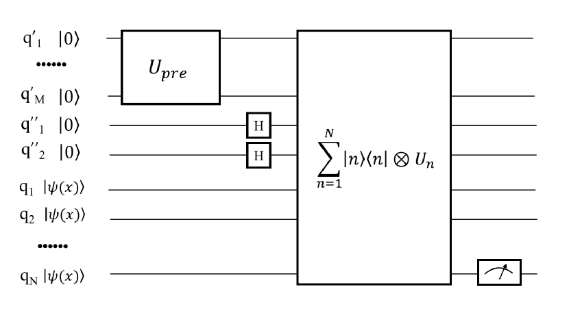
(a)

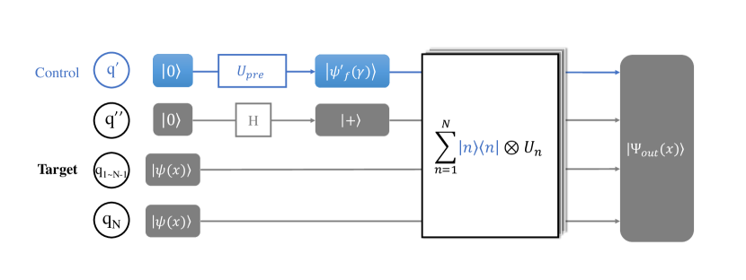
(b)

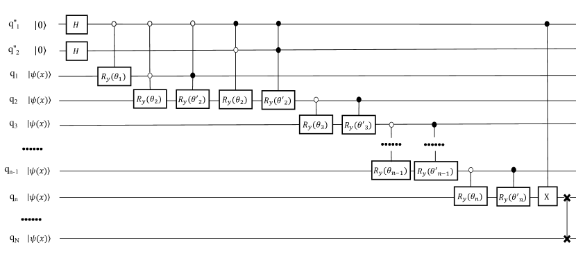
(c)

Figure 1: Sketch of the quantum circuit estimating $F_{N}(x).$
Structure of the whole circuit is shown in fig.(1(a)). There are two main modules. The first one contains $U_{pre}$ acting on the auxiliary qubits $q^{\prime}$, and Hadamard gates acting on $q^{\prime\prime}$. The succeeding module is formed by $N$ controlled unitary operations denoted as $U_{n}$. The corresponding evolution is demonstrated in fig.(1(b)), where $q^{\prime}$ (blue color) are control qubits. $q^{\prime}$ are converted to state $|\psi_{f}^{\prime}(\gamma)\rangle$ under the operation $U_{pre}$, where $\gamma$ is determined by $F_{N}$. The detailed sketch of $U_{n}$ is shown in fig.(1(c)). Initially, Hadamard gates are applied on $q^{\prime\prime}$, and a rotation $Y$ gate is applied on the first qubit $q_{1}$. All these three qubits then acts as control qubits, while $q_{2}$ is the target in following operation. Next, qubits $q_{2},q_{3},\cdots,q_{n}$ are connected as a chain with simple control rotation $Y$ gates. Finally a swap gate between $q_{n}$ and $q_{N}$ is included, ensuring that all the necessary information are stored in the last qubit $q_{N}$.

Thus, subsequent to the whole operation, the output state will be

$$\begin{split}|\Psi_{out}(x)\rangle=\sqrt{-CF_{N}(x)+\frac{1}{2}}|\phi_{0}\rangle_{q^{\prime},q^{\prime\prime},q_{1},\cdots,q_{N-1}}\otimes|0\rangle_{q_{N}}+\sqrt{CF_{N}(x)+\frac{1}{2}}|\phi_{1}\rangle_{q^{\prime},q^{\prime\prime},q_{1},\cdots,q_{N-1}}\otimes|1\rangle_{q_{N}}\end{split}$$ (8)

where $|\phi_{0,1}\rangle$ describing output state of all qubits and auxiliary qubits except the last one $q_{N}$. Hence, information stored in $q_{N}$ is essential and sufficient. After measuring $q_{N}$, the probability of getting $|1\rangle$ is an estimation of $F_{N}(x)$. Whereas, it is also appropriate to apply succeeding operations on $q_{N}$, regarding it as an intermediate state for further computation. The same quantum circuit structure works when the input is in a superposition states, namely $|\Psi_{in}^{s}({\bf x})\rangle$ describing a vector ${\bf x}$ that contains $L+1$ components,

$$|\Psi_{in}^{s}({\bf x})\rangle=\sum_{l=0}^{L}{c_{l}|\Psi_{in}(x_{l})\rangle_{q^{\prime},q^{\prime\prime},q}\otimes|\Phi_{l}\rangle_{Q}}$$ (9)

where $q^{\prime},q^{\prime\prime},q$ are entangled with some other qubits, namely in $Q$. The superscript $s$ represents superposition, subscripts $q^{\prime},q^{\prime\prime},q$ and $Q$ indicate the group of different qubits in different registers, and $\sum_{l=0}^{L}{|c_{l}|}^{2}=1$. $|\Phi_{l}\rangle$ is a complete orthogonal set of the subspace expanded by $Q$, ensuring that $\langle\Phi_{l^{\prime}}|\Phi_{l}\rangle=\delta_{l^{\prime}l}$. After the whole operation, the output state is given by

$$|\Psi_{out}^{s}({\bf x})\rangle=\sum_{l=0}^{L}{c_{l}|\Psi_{out}(x_{l})\rangle_{q^{\prime},q^{\prime\prime},q}\otimes|\Phi_{l}\rangle_{Q}}$$

If we only focus on the subspace expanded by $q_{N}$ and $Q$,

$$|\Psi_{out}^{s}({\bf x})\rangle_{q_{N},Q}=\sum_{l=1}^{L}{c_{l}\left[\sqrt{-CF_{N}(x_{l})+\frac{1}{2}}|0\rangle_{q_{N}}+\sqrt{CF_{N}(x_{l})+\frac{1}{2}}|1\rangle_{q_{N}}\right]\otimes|\Phi_{l}\rangle_{Q}}$$ (10)

Then if $q_{N}$ is measured, probability to get result $|1\rangle$ will be $\frac{1}{2}+C\sum_{l=0}^{L}|c_{l}|^{2}F_{N}(x_{l})\frac{1}{2}$. This property leads to potential applications in quantum algorithm development, for example, the design of nonlinear activation between layers in quantum machine learning.

2 Implementation: Simulation for the square wave function

In this section we will demonstrate the quantum circuit design with a trivial example: Simulation of the square wave function. Consider the following Fourier expansion for the square wave function $f(x)=sign(\sin 2x)$, the sum of the first 7 terms is given by,

$$F(x)=\sum_{n=1\in odd}^{7}\frac{1}{n}\cos\left[n\cdot 2x-\frac{\pi}{2}\right]$$ (11)

where $F(x)$ is an odd function with $a_{2,4,6}=0$. $q_{1,\cdots,7}$ are required carrying out the input information, all of which will be initially prepared in the state $|\psi(x)\rangle$. Additionally, we need 5 auxiliary qubits, denoting them as $q^{\prime}_{1,2},q^{\prime\prime}_{1,2,3}$, and $a_{n}^{\prime},b_{n}^{\prime}$ satisfy

$$C\sum_{n=1}^{j}a^{\prime}_{n}\cos(2nx+b^{\prime}_{n})=\sum_{n=1}^{N}a_{n}\cos(2nx+b_{n})-\sum_{m=j+1}^{N}\gamma_{m}\alpha^{m}\prod_{k=1}^{m}\cos(2x-\beta_{k}^{m})\qquad 1\leq j<N$$ (12)

Then for $n>1$ we set

$$\left\{\begin{array}[]{lr}\gamma_{n}=\frac{2^{n-1}Ca^{\prime}_{n}}{\alpha^{n}}&\\ \beta_{k}^{n}=-\frac{b^{\prime}_{n}}{n},&b^{\prime}_{n}\neq 0\\ \beta_{k}^{n}=\frac{\pi}{3}\delta_{1,0}-\frac{\pi}{3(n-1)},&b^{\prime}_{n}=0\end{array}\right.$$ (13)

Eq.(13) ensures that $\gamma_{2,4,6}$ are all zero, so that we do not need to construct $U_{2,4,6}$ in the circuit. We need to stress the fact that the above setting is not optimal, especially when one prefer a greater value of $|C|$ instead of a shallow circuit. Fig.(2(a)) is a scheme of the whole operation. Operations in the blue block is $U_{pre}$, which converts $q^{\prime}$ into state $|\psi^{\prime}_{f}(\gamma)\rangle$ in eq.(3). Due to the fact that $\gamma_{2,4,6}$ are all zero, then there is no need for construct $U_{2,4,6}$ in the quantum circuit. As shown in the green block, $U_{1}$ is a single rotation $Y$ gate acts on the last qubit $q_{7}$ directly. The other $U_{n}$ acts on $q^{\prime\prime}_{1,2}$, $q_{1,2,\cdots,j}$ and $q_{7}$. For illustration, we only plot details of $U_{3}$, as shown in the yellow block. Based on eq.(7), eq.(11) can be rewritten as

$$\begin{split}F(x)=&-0.8211\cdot\cos(2x-4.8812)+18.9339\cdot\cos^{3}(2x-0.2384)\\ &-15.6030\cdot\cos^{5}(2x-0.0046)-9.1429\cdot\cos^{7}(2x-0.6732)\end{split}$$

Contributions of each single operation $U_{j}$ alone is shown in fig.(2(b)). The sum of all their contributions are shown in fig.(2(c)), which is the output result. $P_{1}$ is probability to get the outcome result $|1\rangle$ when measuring the last qubit $q_{7}$ after the whole operation. Fig.(2(d)) is a sketch of the connectivity structure. Each node represents a single qubit. If two qubits are connected via a blue curve, then there is at least one 2-qubit gate acting on them. All auxiliary qubits $q^{\prime}$ and $q^{\prime\prime}$ are connected with each other. Meanwhile, all qubits $q$ are connected to all of the other auxiliary qubits. For any $1\leq n<N$, there is also a connection between $q_{n}$ and its neighbor $q_{n+1}$. The last qubit $q_{N}$ is connected to all other qubits.

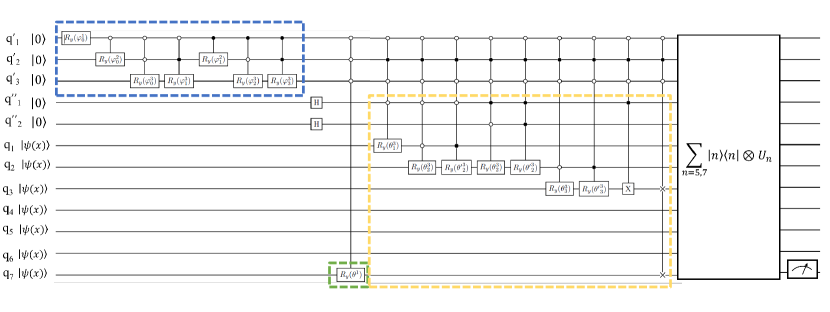
(a)

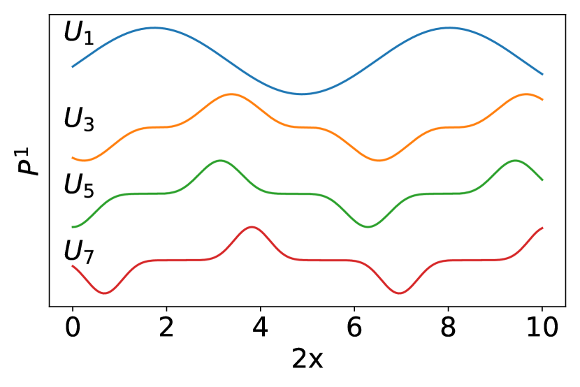
(b)

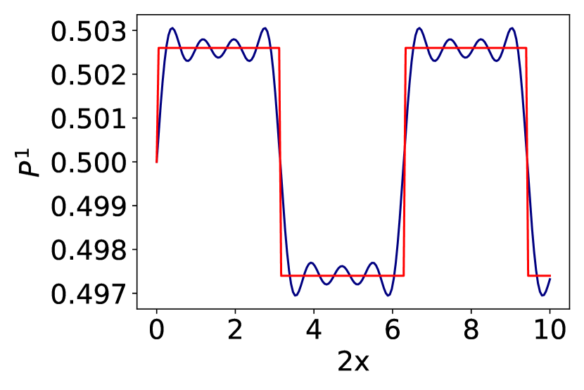
(c)

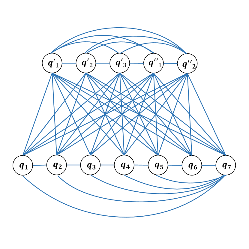
(d)

Figure 2: The quantum circuit estimating 1-D square wave function.
Fig.(2(a)) is a sketch of the quantum circuit estimating square wave function. Operations in the blue block is $U_{pre}$, which converts $q^{\prime}$ into state $|\psi^{\prime}_{f}(\gamma)\rangle$ in eq.(3). Due to the fact that $\gamma_{2,4,6}$ are all zero, $U_{2,4,6}$ disappears in the circuit. As shown in the green block, $U_{1}$ is a single rotation $Y$ gate acts on the last qubit $q_{7}$ directly. The other $U_{n}$ acts on $q^{\prime\prime}_{1,2}$, qubits $q_{1,2,\cdots,j}$ and $q_{7}$. Attributable to the space, here we only plot details of $U_{3}$, as shown in the yellow block. Numerical simulation results are included in fig.(2(b),2(c)). $P_{1}$ is probability to get result $|1\rangle$ when measuring the last qubit $q_{7}$ after the whole operation. $x$ is the variable in the input state $|\psi(x)\rangle$. Contributions of each single operation $U_{j}$ alone is shown in fig.(2(b)). Amplitudes are not included when plotting fig.(2(b)). In fig.(2(c)), the blue curve represents the sum of contributions of all $U_{1,3,5,7}$, which is as well the expected result when measuring $q_{7}$. Meanwhile, the red curve is the original shape of square wave functions. Fig.(2(d)) is a sketch of the connectivity structure. Each node represents a single qubit. If two qubits are connected via a blue curve, then there is at least one 2-qubit gate acting on them.

Further, we also implemented $U_{3,5,7}$ independently based on IBM QASM simulator, as shown in fig.(3), where for each single dot we collect data from 8192 iterative measurements. Results from IBM QASM simulator fit well with the theoretical prediction corresponding to $U_{3}$ and $U_{5}$, as shown in fig.(3(b)) and fig.(3(c)). More details of the simulations can be found in the supplementary materials.

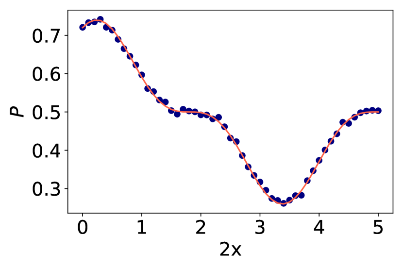
(a)

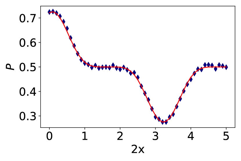
(b)

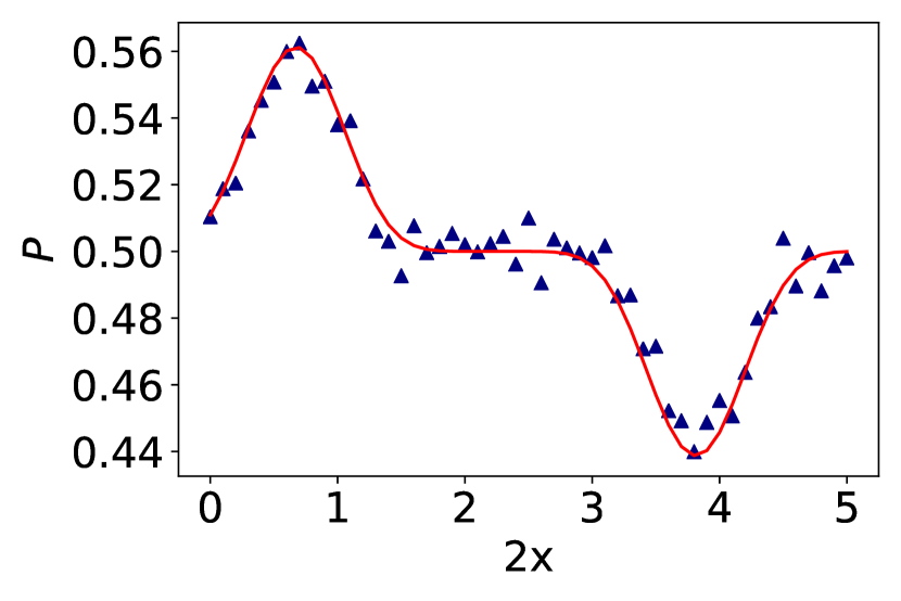
(c)

Figure 3: Implementation on IBM QASM simulator.
Fig.(3(a)) is numerical simulation results of $U_{3}$, contributing component $\cos^{3}(2x-0.2384)$, while fig.(3(b)) and fig.(3(c)) corresponds to $U_{5}$ and $U_{7}$, calculating components $\cos^{5}(2x-0.0046)$ and $\cos^{7}(2x-0.6732)$. Red lines represent the theoretical prediction, and blue dots(or diamonds, triangles) represent the results on IBM QASM simulator. $P$ is the probability to get state $|0\rangle$ or $|1\rangle$ when measuring the last qubit. (Generally, we prefer to get state $|1\rangle$ when calculating a positive component in the expansion, and $|0\rangle$ when calculating a negative one.) For each single dot we collect data from 8192 iterative measurements.

3 Time complexity

We will compare the time complexity for three various situations: In the first situation we consider classical inputs, while for others we consider some unknown quantum states as inputs. One can either estimate $x$ from the input and calculate $F_{N}(x)$ classically, or apply the method presented in this article to estimate the outputs.

Situation I. Estimate $F_{N}(x)$ with a classical input $x$:

To estimate a periodic function $F_{N}(x)$ within error $\epsilon$, $O(\frac{1}{\epsilon})$ times of measurement are required[43]. Initially $N$ $R_{y}$ rotation gates are required for mapping $x$ into quantum state $|\psi(x)\rangle^{\otimes N}$. Moreover, we need $M+2$ auxiliary qubits, where $M=\lceil\log_{2}N\rceil$ for control qubits. $U_{pre}$ contains $O(exp(M))$ multi control gates, and in each of them there are at most $M-1$ control qubits. The time scaling of n-control gates is $O(n^{2})$[44], thus the time complexity of $U_{pre}$ is $O(N\lceil\log_{2}N\rceil^{2})$.

Consider the basic unit $U_{n}$. When $n>2$, there are $4$ Control-Control rotation gates, $4n-8$ control-rotation gates and one optional 2-qubit swap gate. Thus, it takes time $O(n\lceil\log_{2}n\rceil^{2})$ to implement the operation $|n\rangle\langle n|\otimes U_{n}$. After taking the $M$ auxiliary qubits into account, $M$ control qubits are added to all gates in $U_{n}$. Therefore, it takes time $O(n)$ to achieve a single $U_{n}$ Notice that there are $N$ similar $U_{n}$, where $n=1,2,\cdots,N$, time complexity to finish all $\sum_{n=1}^{N}|n\rangle\langle n|\otimes U_{n}$ is $O(N^{2}\lceil\log_{2}N\rceil^{2})$.

Totally, to derive the estimation $CF_{N}(x)$ within error $\epsilon$, the time complexity is of order $O(N^{2}\lceil\log_{2}N\rceil^{2}/\epsilon)$, which is still polynomial. On the other hand, time complexity to estimate $F_{N}(x)$ for a single $x$ based on Taylor expansion is also polynomial to $N$. Hence under this situation there is no speedup comparing with the classical calculation.

Situation II. Estimate $F_{N}(x)$ with input quantum state $|\psi(x)\rangle^{\otimes N}$, where the value of $x$ is still unknown:

The only difference from the previous situation is that the mapping process now can be skipped. Still, time consuming is of order $O(N^{2}\lceil\log_{2}N\rceil^{2}/\epsilon)$. By contrast, to calculate $F_{N}(x)$ from $|\psi(x)\rangle^{\otimes N}$ classically, the first step is to derive $x$ from the input states. It requires $O(\frac{1}{\epsilon})$ measurements to get $\cos x$ within error $\epsilon$, and then the time complexity to estimate $F_{N}(x)$ is polynomial to $N$. Still, under this situation there is no speedup comparing with the classical calculation.

Situation III. Estimate $\sum_{l=0}^{L}|c_{l}|^{2}F_{N}(x_{l})$ with input quantum state $|\Psi_{in}^{s}({\bf x})\rangle$, as described in eq.(9):

Here we denote $N^{\prime}$ as the number of qubits that form state $|\Phi\rangle$, and $L=2^{N^{\prime}}-1$. Even though more variables are introduced into the input, we do not need to change anything in the quantum circuit. To get an estimation of $C\sum_{l=0}^{L}|c_{l}|^{2}F_{N}(x_{l})$ with the quantum method, time consuming is still of order $O(N^{2}\lceil\log_{2}N\rceil^{2}/\epsilon)$, which does not depend on the scale of $N^{\prime}$(Number of qubits in $Q$). However, in the classical method, as $c_{j}$ are unknown initially, one must estimate them before calculating $\sum_{l=0}^{L}|c_{l}|^{2}F_{N}(x_{j})$. Time complexity of quantum tomography is exponential in $N^{\prime}$, or at least polynomial in $N^{\prime}$ with shadow quantum tomography. The time complexity of quantum method is only determined by $N$, while the classical method is at least polynomial in $N^{\prime}$[45]. Thus, when $N^{\prime}>>N$, the quantum method will lead to polynomial speedup comparing with the classical one.

Consider the task to estimate $|c_{0}|^{2}F(x_{0})+|c_{1}|^{2}F(x_{1})$, where $|c_{0}|^{2}+|c_{1}|^{2}=1$. For simplicity, here we set $F(x)=cos^{3}(x-0.2384)$, which can be implemented by $U_{3}$ itself, excluding the $q^{\prime}$ registers. (Structure of $U_{3}$ can be found in Fig.(2) in the main article and Fig.(S2) in the SM.) In Situation III, the input states $|\Psi_{in}^{s}({\bf x})\rangle$ can be described by Eq.(9).

In the task estimating $|c_{0}|^{2}F(x_{0})+|c_{1}|^{2}F(x_{1})$, we only need one qubit as $Q$ preparing the initial states. A sketch of the quantum circuit calculating $|c_{0}|^{2}F(x_{0})+|c_{1}|^{2}F(x_{1})$ is shown in Fig.(4). There are totally 6 qubits, $q^{\prime\prime}_{1,2}$ and $q_{1,2,3}$ implementing $U_{3}$, and qubit $Q$ corresponding to Eq.(9). Initially, all qubits are set as $|0\rangle$. Operations in the dashed blue square converts them into state

$$|\Psi_{in}^{s}(x_{0},x_{1})\rangle=c_{0}|\Psi_{in}(x_{0})\rangle_{q^{\prime},q^{\prime\prime},q}\otimes|0\rangle_{Q}+c_{1}|\Psi_{in}(x_{1})\rangle_{q^{\prime},q^{\prime\prime},q}\otimes|1\rangle_{Q}$$ (14)

where $|\Psi_{in}(x)\rangle_{q^{\prime},q^{\prime\prime},q}=|0\rangle^{\otimes 2}_{q^{\prime}}\otimes|\psi(x)\rangle^{\otimes 3}_{q}$, and $|\psi(x)\rangle=\cos x|0\rangle+\sin x|1\rangle$. Coefficients $c_{0,1}$ are determined by the gate $R_{y}(\theta_{sup})$ acting on $Q$, leading to

$$c_{0}=\cos(\frac{\theta_{sup}}{2})$$

$$c_{1}=\sin(\frac{\theta_{sup}}{2})$$

Then, operation $U_{3}$ is applied on $q^{\prime}$ and $q$, implementing the calculation of $F(x)$. After the whole operations, the output state is given by

$$|\Psi_{out}^{s}({x_{0},x_{1}})\rangle=c_{0}|\Psi_{out}(x_{0})\rangle_{q^{\prime},q^{\prime\prime},q}\otimes|0\rangle_{Q}+c_{1}|\Psi_{out}(x_{1})\rangle_{q^{\prime},q^{\prime\prime},q}\otimes|1\rangle_{Q}$$

where $|\Psi_{out}(x)\rangle$ is described by Eq.(8).

In this example, $P_{0}$, which represents the probability to get result $|0\rangle$ when measuring $q_{3}$, can be calculated as

$$P_{0}=\cos^{2}(\frac{\theta_{sup}}{2})[0.2362\cos^{3}(2x_{0}-0.2384)+0.5]+\sin^{2}(\frac{\theta_{sup}}{2})[0.2362\cos^{3}(2x_{1}-0.2384)+0.5]$$ (15)

Thus, we only need to measure $q_{3}$ itself to estimate $|c_{0}|^{2}F(x_{0})+|c_{1}|^{2}F(x_{1})$.

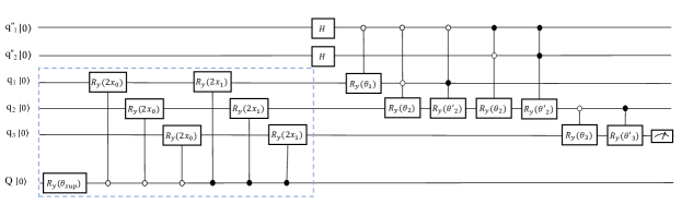
Figure 4: A sketch of the quantum circuit that calculates $|c_{0}|^{2}F(x_{0})+|c_{1}|^{2}F(x_{1})$.
There are totally 6 qubits, $q^{\prime\prime}_{1,2}$ and $q_{1,2,3}$ implementing $U_{3}$, and qubit $Q$ corresponding to Eq.(9). Initially, all qubits are set as $|0\rangle$. Operations in the dashed blue square converts them into state $|\Psi_{in}^{s}(x_{0},x_{1})\rangle$, as shown in Eq.(14). Then, operation $U_{3}$ is applied on $q^{\prime}$ and $q$, implementing the calculation of $F(x)$. After the whole operation, we only to measure $q_{3}$ itself to estimate $|c_{0}|^{2}F(x_{0})+|c_{1}|^{2}F(x_{1})$. $P_{0}$, the probability to get result $|0\rangle$ when measuring $q_{3}$ is presented in Eq.(15).

Further, we implement the operation shown in Fig.(4) on IBM QASM simulator. Simulation results obtained from IBM QASM simulator are shown in Fig.(5(b)), where $P_{0}$ indicates the probability to get result $|0\rangle$ when measuring $q_{3}$ after the whole operation. Blue dots or diamonds represent the simulation results from IBM QASM simulator, while the red curve is theoretical prediction based on Eq.(15). In Fig.(5(a)), we set $x_{0}=0$, $\theta_{sup}=\pi$, and collect $P_{0}$ under various $x_{1}$ values. $P_{0}$ shows the shape of $F(x_{1})$, as we set $\theta_{sup}=\pi$ so that $x_{0}$ has no contribution to $P_{0}$. In Fig.(5(b)), we set $x_{0}=3.4$, $x_{1}=0.2$, and collect $P_{0}$ under various $\theta_{sup}$ values. Theoretically $P_{0}$ should have a single sin function shape, and the simulation results fit the prediction very well. For each single dot we collect data from 8192 iterative measurements.

In the simulation only one qubit, $q_{3}$, is measured, and $|c_{0}|^{2}F(x_{0})+|c_{1}|^{2}F(x_{1})$ can be estimated from $P_{0}$, the probability to get result $|0\rangle$. Therefore, with the quantum algorithm as we proposed, we do not need to estimate the exact values of $c_{l}$, so that the quantum method leads to speedup comparing with the classical version in situation III, especially when $L$ is large.

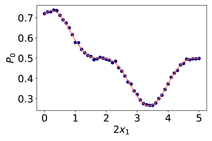
(a)

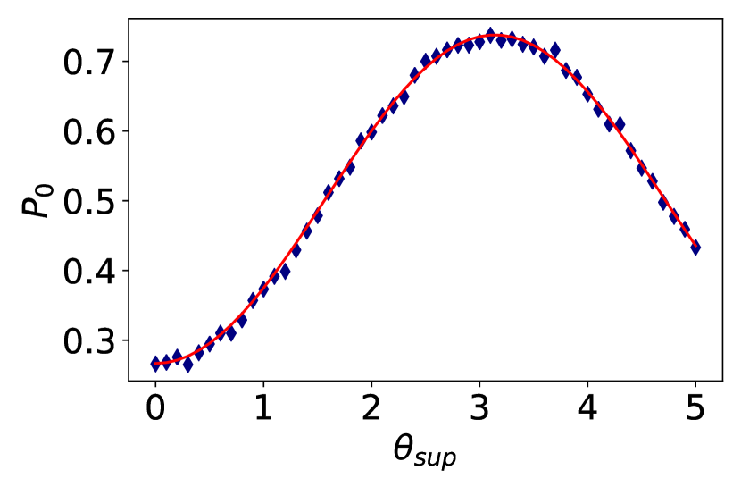
(b)

Figure 5: Implementation on IBM QASM simulator.
Here we present the simulation results obtained from IBM QASM simulator. In both figures $P_{0}$ indicates the probability to get result $|0\rangle$ when measuring $q_{3}$ after the whole operation shown in Fig.(4). Blue dots or diamonds represent the simulation results from IBM QASM simulator, while the red curve is theoretical prediction based on Eq.((15)). In Fig.(5(a)), we set $x_{0}=0$, $\theta_{sup}=\pi$, and collect $P_{0}$ under various $x_{1}$ values. $P_{0}$ shows the shape of $F(x_{1})$, as we set $\theta_{sup}=\pi$ so that $x_{0}$ has no contribution to $P_{0}$. In Fig.(5(b)), we set $x_{0}=3.4$, $x_{1}=0.2$, and collect $P_{0}$ under various $\theta_{sup}$ values. Theoretically $P_{0}$ should have a single sin function shape, and the simulation results fit the prediction very well. For each single dot we collect data from 8192 iterative measurements.

4 Conclusion

Here, we propose a universal quantum circuit design for any arbitrary one-dimensional periodic function. The inputs are sufficient qubits prepared at the same state, while the last one will represent the output outcome. One can either estimate the exact value from repeating measurements on the last qubit, or regard it as an intermediate state prepared for succeeding operations. Superposition in the input leads to similarly superposition in the output, which leads to speedup under some certain circumstances, especially when dealing with unknown quantum inputs. As an simple example we illustrate the quantum circuit design for the square wave function. Both exact simulations and implementation on IBM-QASM gave very accurate result and illustrate the power of this proposed general design. This general approach might be used to construct an appropriate quantum circuit for the electronic wave function in periodic solids and materials, moreover in quantum machine learning particularly simulating the non-linear function used in the network.

References

- [1] Frank Arute, Kunal Arya, Ryan Babbush, Dave Bacon, Joseph C Bardin, Rami Barends, Rupak Biswas, Sergio Boixo, Fernando GSL Brandao, David A Buell, et al. Quantum supremacy using a programmable superconducting processor. Nature, 574(7779):505–510, 2019.
- [2] John Preskill. Quantum computing in the nisq era and beyond. Quantum, 2:79, 2018.
- [3] Han-Sen Zhong, Hui Wang, Yu-Hao Deng, Ming-Cheng Chen, Li-Chao Peng, Yi-Han Luo, Jian Qin, Dian Wu, Xing Ding, Yi Hu, et al. Quantum computational advantage using photons. Science, 370(6523):1460–1463, 2020.
- [4] Nikolaj Moll, Panagiotis Barkoutsos, Lev S Bishop, Jerry M Chow, Andrew Cross, Daniel J Egger, Stefan Filipp, Andreas Fuhrer, Jay M Gambetta, Marc Ganzhorn, et al. Quantum optimization using variational algorithms on near-term quantum devices. Quantum Science and Technology, 3(3):030503, 2018.
- [5] Leo Zhou, Sheng-Tao Wang, Soonwon Choi, Hannes Pichler, and Mikhail D Lukin. Quantum approximate optimization algorithm: Performance, mechanism, and implementation on near-term devices. Physical Review X, 10(2):021067, 2020.
- [6] Jian Pan, Yudong Cao, Xiwei Yao, Zhaokai Li, Chenyong Ju, Hongwei Chen, Xinhua Peng, Sabre Kais, and Jiangfeng Du. Experimental realization of quantum algorithm for solving linear systems of equations. Physical Review A, 89(2):022313, 2014.
- [7] Hsin-Yuan Huang, Kishor Bharti, and Patrick Rebentrost. Near-term quantum algorithms for linear systems of equations. arXiv preprint arXiv:1909.07344, 2019.
- [8] Leonard Wossnig, Zhikuan Zhao, and Anupam Prakash. Quantum linear system algorithm for dense matrices. Physical review letters, 120(5):050502, 2018.
- [9] Zhen Huang, Hefeng Wang, and Sabre Kais. Entanglement and electron correlation in quantum chemistry calculations. Journal of Modern Optics, 53(16-17):2543–2558, 2006.
- [10] Abhinav Kandala, Antonio Mezzacapo, Kristan Temme, Maika Takita, Markus Brink, Jerry M Chow, and Jay M Gambetta. Hardware-efficient variational quantum eigensolver for small molecules and quantum magnets. Nature, 549(7671):242–246, 2017.
- [11] Rongxin Xia, Teng Bian, and Sabre Kais. Electronic structure calculations and the ising hamiltonian. The Journal of Physical Chemistry B, 122(13):3384–3395, 2017.
- [12] Robert M Parrish, Edward G Hohenstein, Peter L McMahon, and Todd J Martínez. Quantum computation of electronic transitions using a variational quantum eigensolver. Physical review letters, 122(23):230401, 2019.
- [13] Teng Bian and Sabre Kais. Quantum computing for atomic and molecular resonances. The Journal of Chemical Physics, 154(19):194107, 2021.
- [14] Rongxin Xia and Sabre Kais. Hybrid quantum-classical neural network for calculating ground state energies of molecules. Entropy, 22(8):828, 2020.
- [15] Rongxin Xia and Sabre Kais. Qubit coupled cluster singles and doubles variational quantum eigensolver ansatz for electronic structure calculations. Quantum Science and Technology, 6(1):015001, 2020.
- [16] Zixuan Hu and Sabre Kais. A quantum encryption scheme featuring confusion, diffusion, and mode of operation. arXiv preprint arXiv:2010.03062, 2020.
- [17] Junxu Li, Zixuan Hu, and Sabre Kais. A practical quantum encryption protocol with varying encryption configurations. arXiv preprint arXiv:2101.09314, 2021.
- [18] Alberto Peruzzo, Jarrod McClean, Peter Shadbolt, Man-Hong Yung, Xiao-Qi Zhou, Peter J Love, Alán Aspuru-Guzik, and Jeremy L O’brien. A variational eigenvalue solver on a photonic quantum processor. Nature communications, 5(1):1–7, 2014.
- [19] Jarrod R McClean, Jonathan Romero, Ryan Babbush, and Alán Aspuru-Guzik. The theory of variational hybrid quantum-classical algorithms. New Journal of Physics, 18(2):023023, 2016.
- [20] Ramiro Sagastizabal, Xavier Bonet-Monroig, Malay Singh, M Adriaan Rol, CC Bultink, Xiang Fu, CH Price, VP Ostroukh, N Muthusubramanian, A Bruno, et al. Experimental error mitigation via symmetry verification in a variational quantum eigensolver. Physical Review A, 100(1):010302, 2019.
- [21] Ilya G Ryabinkin, Scott N Genin, and Artur F Izmaylov. Constrained variational quantum eigensolver: Quantum computer search engine in the fock space. Journal of chemical theory and computation, 15(1):249–255, 2018.
- [22] Ken M Nakanishi, Kosuke Mitarai, and Keisuke Fujii. Subspace-search variational quantum eigensolver for excited states. Physical Review Research, 1(3):033062, 2019.
- [23] Julio T Barreiro, Markus Müller, Philipp Schindler, Daniel Nigg, Thomas Monz, Michael Chwalla, Markus Hennrich, Christian F Roos, Peter Zoller, and Rainer Blatt. An open-system quantum simulator with trapped ions. Nature, 470(7335):486–491, 2011.
- [24] Zixuan Hu, Rongxin Xia, and Sabre Kais. A quantum algorithm for evolving open quantum dynamics on quantum computing devices. Scientific reports, 10(1):1–9, 2020.
- [25] Scott E Smart and David A Mazziotti. Quantum solver of contracted eigenvalue equations for scalable molecular simulations on quantum computing devices. Physical Review Letters, 126(7):070504, 2021.
- [26] Kade Head-Marsden, Stefan Krastanov, David A Mazziotti, and Prineha Narang. Capturing non-markovian dynamics on near-term quantum computers. Physical Review Research, 3(1):013182, 2021.
- [27] James A Pauls, Yiteng Zhang, Gennady P Berman, and Sabre Kais. Quantum coherence and entanglement in the avian compass. Physical review E, 87(6):062704, 2013.
- [28] Rongxin Xia and Sabre Kais. Quantum machine learning for electronic structure calculations. Nature communications, 9(1):1–6, 2018.
- [29] Jacob Biamonte, Peter Wittek, Nicola Pancotti, Patrick Rebentrost, Nathan Wiebe, and Seth Lloyd. Quantum machine learning. Nature, 549(7671):195–202, 2017.
- [30] Maria Schuld and Nathan Killoran. Quantum machine learning in feature hilbert spaces. Physical review letters, 122(4):040504, 2019.
- [31] William Huggins, Piyush Patil, Bradley Mitchell, K Birgitta Whaley, and E Miles Stoudenmire. Towards quantum machine learning with tensor networks. Quantum Science and technology, 4(2):024001, 2019.
- [32] Vivek Dixit, Raja Selvarajan, Tamer Aldwairi, Yaroslav Koshka, Mark A Novotny, Travis S Humble, Muhammad A Alam, and Sabre Kais. Training a quantum annealing based restricted boltzmann machine on cybersecurity data. IEEE Transactions on Emerging Topics in Computational Intelligence, 2021.
- [33] Sayan Roy, Zixuan Hu, Sabre Kais, and Peter Bermel. Enhancement of photovoltaic current through dark states in donor-acceptor pairs of tungsten-based transition metal di-chalcogenides. Advanced Functional Materials, page 2100387, 2021.
- [34] Manas Sajjan, Shree Hari Sureshbabu, and Sabre Kais. Quantum machine-learning for eigenstate filtration in two-dimensional materials. arXiv preprint arXiv:2105.09488, 2021.
- [35] Blake A Wilson, Zhaxylyk A Kudyshev, Alexander V Kildishev, Sabre Kais, Vladimir M Shalaev, and Alexandra Boltasseva. Machine learning framework for quantum sampling of highly-constrained, continuous optimization problems. arXiv preprint arXiv:2105.02396, 2021.
- [36] Moshe Leshno, Vladimir Ya Lin, Allan Pinkus, and Shimon Schocken. Multilayer feedforward networks with a nonpolynomial activation function can approximate any function. Neural networks, 6(6):861–867, 1993.
- [37] Mitja Peruš. Neural networks as a basis for quantum associative networks. Neural Netw. World, 10(6):1001–1013, 2000.
- [38] Michail Zak and Colin P Williams. Quantum neural nets. International journal of theoretical physics, 37(2):651–684, 1998.
- [39] Yudong Cao, Gian Giacomo Guerreschi, and Alán Aspuru-Guzik. Quantum neuron: an elementary building block for machine learning on quantum computers. arXiv preprint arXiv:1711.11240, 2017.
- [40] Maria Schuld, Ilya Sinayskiy, and Francesco Petruccione. Simulating a perceptron on a quantum computer. Physics Letters A, 379(7):660–663, 2015.
- [41] Don Coppersmith. An approximate fourier transform useful in quantum factoring. arXiv preprint quant-ph/0201067, 2002.
- [42] Yaakov S Weinstein, MA Pravia, EM Fortunato, Seth Lloyd, and David G Cory. Implementation of the quantum fourier transform. Physical review letters, 86(9):1889, 2001.
- [43] András Gilyén, Yuan Su, Guang Hao Low, and Nathan Wiebe. Quantum singular value transformation and beyond: exponential improvements for quantum matrix arithmetics. In Proceedings of the 51st Annual ACM SIGACT Symposium on Theory of Computing, pages 193–204, 2019.
- [44] Adriano Barenco, Charles H Bennett, Richard Cleve, David P DiVincenzo, Norman Margolus, Peter Shor, Tycho Sleator, John A Smolin, and Harald Weinfurter. Elementary gates for quantum computation. Physical review A, 52(5):3457, 1995.
- [45] Scott Aaronson. Shadow tomography of quantum states. SIAM Journal on Computing, 49(5):STOC18–368, 2019.