\newsiamremark

remarkRemark \newsiamremarkhypothesisHypothesis \newsiamthmclaimClaim \headersSingular DMDJ. A. Rosenfeld and R. Kamalapurkar \externaldocumentex_supplement \useunder\ul \useunder\ul

Singular Dynamic Mode Decompositionsthanks: A YouTube playlist to accompany this work may be found at: https://youtube.com/playlist?list=PLldiDnQu2phsZdFP3nHoGnk_Aq-kp_4nE \fundingThis research was supported by the Air Force Office of Scientific Research (AFOSR) under contract numbers FA9550-20-1-0127 and FA9550-21-1-0134, and the National Science Foundation (NSF) under award numbers 2027976 and 1900364. Any opinions, findings and conclusions or recommendations expressed in this material are those of the author(s) and do not necessarily reflect the views of the sponsoring agencies.

Joel A. Rosenfeld Department of Mathematics and Statistics, University of South Florida, Tampa, FL 33620 USA (, http://thelearningdock.org) rosenfeldj@usf.edu    Rushikesh Kamalapurkar Department of Mechanical and Aerospace Engineering, Oklahoma State University, Stillwater, OK 74078 USA (, https://scc-lab.github.io) rushikesh.kamalapurkar@okstate.edu
Abstract

This manuscript is aimed at addressing several long standing limitations of dynamic mode decompositions in the application of Koopman analysis. Principle among these limitations are the convergence of associated Dynamic Mode Decomposition algorithms and the existence of Koopman modes. To address these limitations, two major modifications are made, where Koopman operators are removed from the analysis in light of Liouville operators (known as Koopman generators in special cases), and these operators are shown to be compact for certain pairs of Hilbert spaces selected separately as the domain and range of the operator. While eigenfunctions are discarded in the general analysis, a viable reconstruction algorithm is still demonstrated, and the sacrifice of eigenfunctions realizes the theoretical goals of DMD analysis that have yet to be achieved in other contexts. However, in the case where the domain is embedded in the range, an eigenfunction approach is still achievable, where a more typical DMD routine is established, but that leverages a finite rank representation that converges in norm. The manuscript concludes with the description of two Dynamic Mode Decomposition algorithms that converges when a dense collection of occupation kernels, arising from the data, are leveraged in the analysis.

1 Introduction

This manuscript is aimed at addressing several long standing limitations of dynamic mode decompositions (DMD) in the application of Koopman analysis. Principle among these limitations are the convergence of associated Dynamic Mode Decomposition algorithms and the existence of Koopman modes, where the first has only been established with respect to the strong operator topology (which does not guarantee the convergence of the spectrum), and the second is only guaranteed to exist when the Koopman operator is compact as well as self-adjoint or normal (which is a rare occurrence over the typical sample spaces).

DMD methods are data analysis methods that aim to decompose a time series corresponding to a nonlinear dynamical system into a collection of dynamic modes [11, 4, 13, 10]. When they are effective, a given time series can be expressed as a linear combination of dynamic modes and exponential functions whose growth rates are derived from the spectrum of a finite rank representation of a particular operator, usually the Koopman operator.

The use of Koopman operators places certain constraints on the continuous time dynamics that can be studied with DMD methods. In particular, Koopman operators analyze continuous time dynamics through a discrete time proxy obtained by fixing a time-step for a continuous time system [12]. However, only a small subset of continuous time dynamics satisfy the forward invariance property necessary to obtain a discretization [16]. Moreover, to establish convergence guarantees for DMD routines, additional structure is required of Koopman operators, where a sequence of finite rank operators converge to Koopman operators in norm only if the Koopman operator is compact [14]. Compactness is rarely satisfied for Koopman operators, where the Koopman operators obtained through discretizations of the simplest dynamical system x˙=0˙𝑥0\dot{x}=0 are the identity operator and are not compact. A partial result has been demonstrated for when Koopman operators are bounded in [10], where a sequence of finite rank operators converge to a Koopman operator in the Strong Operator Topology (SOT). However, SOT convergence does not guarantee convergence of the spectra (cf. [14]), which is necessary for a DMD routine.

There are stronger theoretical difficulties associated with Koopman operators. It has been demonstrated that among the typical Hilbert spaces leveraged in sampling theory, such as the exponential dot product’s [5], the Gaussian RBF’s [8], and the polynomial kernel’s native spaces as well as the classical Paley Wiener space [6], the only discrete time dynamics that yield a bounded Koopman operator are those dynamics that are affine. Hence, depending on the kernel function selected for the approximation of a Koopman operator, a given Koopman operator can at best be expected to be a densely defined operator, which obviates the aforementioned convergence properties.

Another motivation for the use of Koopman operators in the study of continuous time dynamical systems is a heuristic that for small timesteps the spectra and eigenfunctions of the resultant Koopman operator should be close to that of the Liouville operator representing the continuous time systems [3]. However, for two fixed timesteps, the corresponding Koopman operators can have different collections of eigenfunctions and eigenvalues, and these are artifacts of the discretization itself [8]. Since in most cases the Koopman operators are used for this analysis, it is not clear if there is a method for distinguishing which of these eigenfunctions and eigenvalues are a product of the discretization and which are fundamental to the dynamics themselves.

Finally, and perhaps most alarming, is that Koopman modes themselves exist for only a small subset of Koopman operators [8]. Specifically, if a Koopman operator is self-adjoint, then it admits an orthonormal basis of eigenfunctions [3], and the projection of the full state observable onto this basis yields a collection of (vector valued) coefficients attached to these basis functions. These coefficients are known as Koopman Modes or Dynamic Modes. Koopman operators are not necessarily diagonalizable over a given Hilbert space, and when they are diagonalizable, their complete eigenbasis is not always an orthogonal basis. Hence, as the full state observable is projected on larger and larger finite collections of eigenfunctions, the weights attached to each eigenfunction will change as more are added. This adjustment to the weights with the addition of more eigenfunctions is why a series expansion is only ever given in Hilbert space theory when there is an orthonormal basis of eigenfunctions, otherwise an expansion is written as limit of finite linear combinations of eigenfunctions [14].111There are notable exceptions, such as in atomic decompositions [19]. However, this is another rare property of a basis.

To address these limitations, two major modifications are made, where Koopman operators are removed from the analysis in light of Liouville operators (known as Koopman generators in special cases), and these operators are shown to be compact for certain pairs of Hilbert spaces selected separately as the domain and range of the operator. (This separation of the domain and range is not possible for Koopman operators.) While eigenfunctions are discarded in the general analysis, a viable reconstruction algorithm is still achievable, and the sacrifice of eigenfunctions realizes the theoretical goals of DMD analysis that have yet to be achieved in other contexts. It should be noted that Liouville and Koopman operators rarely admit a diagonalization, and as such, this approach discards that additional assumption on the operators.

However, at the cost of well defined Dynamic Modes, an eigenfunction approach is still achievable when the domain is embedded in the range of the operator. This allows for the search of eigenfunctions through finite rank approximations that converge to the Liouville operator. The result is a norm convergence DMD routine (using eigenfunctions), which is an achievement over the SOT convergent results previously established in the field [10]. This gives a balance between the two convergence methods presented in this manuscript, where well defined modes come at the price of ease of reconstruction, and a straightforward reconstruction algorithm may not have well defined limiting dynamic modes (a problem shared with all other DMD routines).

To be explicit, the singular DMD approach yields the following benefits:

  1. 1.

    Eliminates the requirement of forward invariance. (Aligning with the method given in [17]).

  2. 2.

    Provides well defined Dynamic Modes.

  3. 3.

    Approximates a compact operator, thereby achieving convergence.

  4. 4.

    Yields an orthonormal basis through which the full state observable may be decomposed.

However, this achievement comes at the expense of eigenfunctions of the given operator. As it turns out, the abandonment of eigenfunctions for the analysis does not actually limit the applicability, where even for very simple dynamics, such as f(x)=x2𝑓𝑥superscript𝑥2f(x)=x^{2} in the one dimensional setting, the corresponding Liouville operators will have no eigenfunctions over any space of continuous functions. For the present example, the solution to the eigenfunction equation, g(x)x2=λg(x)superscript𝑔𝑥superscript𝑥2𝜆𝑔𝑥g^{\prime}(x)x^{2}=\lambda g(x), gives g(x)=eλ/x𝑔𝑥superscript𝑒𝜆𝑥g(x)=e^{\lambda/x} for λ0𝜆0\lambda\neq 0, a discontinuous function on the real line. Additionally, reconstruction of the original time series may still be achieved using Runge-Kutta like methods.

Where the DMD routine leveraging the case where the domain is embedded in the range provides the following:

  1. 1.

    Eliminates the requirement of forward invariance. (Aligning with the method given in [17]).

  2. 2.

    Approximates a compact operator, thereby achieving convergence.

  3. 3.

    Yields an approximate eigenbasis through which the full state observable may be decomposed.

  4. 4.

    An ease of reconstruction through the eigenfunctions.

It should be noted that there have been several attempts at providing compact operators for the study of DMD. The approaches [7] and [16] find compact operators through the multiplication of auxiliary operator against Koopman and Liouville operators respectively. However, the resultant operators are not the operators that truly correspond to the dynamics in question, and as such, the decomposition of those operators can only achieve heuristic results. The approach taken presently gives compact Liouville operators directly connected with the continuous time dynamics.

2 Reproducing Kernel Hilbert Spaces

A reproducing kernel Hilbert space (RKHS), H𝐻H, over a set X𝑋X is a space of functions from X𝑋X to \mathbb{R} such that the functional of evaluation, Exg:=g(x)assignsubscript𝐸𝑥𝑔𝑔𝑥E_{x}g:=g(x) is bounded for every xX𝑥𝑋x\in X. By the Riesz theorem, this means for each xX𝑥𝑋x\in X there exists a function KxHsubscript𝐾𝑥𝐻K_{x}\in H such that f,KxH=f(x)subscript𝑓subscript𝐾𝑥𝐻𝑓𝑥\langle f,K_{x}\rangle_{H}=f(x) for all f𝑓f. The function Kxsubscript𝐾𝑥K_{x} is called the kernel function centered at X𝑋X, and the function K(x,y):=Ky,KxHassign𝐾𝑥𝑦subscriptsubscript𝐾𝑦subscript𝐾𝑥𝐻K(x,y):=\langle K_{y},K_{x}\rangle_{H} is called the kernel function corresponding to H𝐻H. Note that Ky(x)=K(x,y).subscript𝐾𝑦𝑥𝐾𝑥𝑦K_{y}(x)=K(x,y). Classical examples of kernel functions in data science are the Gaussian radial basis function for μ>0𝜇0\mu>0, K(x,y)=exp(1μxy2)𝐾𝑥𝑦1𝜇superscriptnorm𝑥𝑦2K(x,y)=\exp(-\frac{1}{\mu}\|x-y\|^{2}), and the exponential dot product kernel, exp(1μxTy)1𝜇superscript𝑥𝑇𝑦\exp(\frac{1}{\mu}x^{T}y) [18].

The function K(x,y)𝐾𝑥𝑦K(x,y) is a positive definite kernel function, which means that for every finite collection of points, {x1,,xM}Xsubscript𝑥1subscript𝑥𝑀𝑋\{x_{1},\ldots,x_{M}\}\subset X, the Gram matrix (K(xi,xj))i,j=1Msuperscriptsubscript𝐾subscript𝑥𝑖subscript𝑥𝑗𝑖𝑗1𝑀(K(x_{i},x_{j}))_{i,j=1}^{M} is positive definite. For each positive definite kernel function, there exists a unique RKHS for which K𝐾K is the kernel function for that space by the Aronszajn-Moore theorem in [1].

Given a RKHS, H𝐻H, over Xn𝑋superscript𝑛X\in\mathbb{R}^{n} consisting of continuous functions and given a continuous signal, θ:[0,T]X:𝜃0𝑇𝑋\theta:[0,T]\to X, the linear functional g0Tg(θ(t))𝑑tmaps-to𝑔superscriptsubscript0𝑇𝑔𝜃𝑡differential-d𝑡g\mapsto\int_{0}^{T}g(\theta(t))dt is bounded. Hence, there exist a function, ΓθHsubscriptΓ𝜃𝐻\Gamma_{\theta}\in H, such that g,ΓθH=0Tg(θ(t))𝑑tsubscript𝑔subscriptΓ𝜃𝐻superscriptsubscript0𝑇𝑔𝜃𝑡differential-d𝑡\langle g,\Gamma_{\theta}\rangle_{H}=\int_{0}^{T}g(\theta(t))dt for all gH𝑔𝐻g\in H. The function ΓθsubscriptΓ𝜃\Gamma_{\theta} is called the occupation kernel in H𝐻H corresponding to θ𝜃\theta. These occupation kernels were first introduced in [17, rosenfeld2019occupation2].

3 Compact Liouville Operators

This section demonstrates the existence of compact Liouville operators, given formally as Afg(x)=g(x)f(x)subscript𝐴𝑓𝑔𝑥𝑔𝑥𝑓𝑥A_{f}g(x)=\nabla g(x)f(x), where compactness is achieved through the consideration of differing spaces for the domain an range of the operator. Section 3.1 builds on a classical result where differentiation between differing weighted Hardy spaces can be readily shown to be compact. Following a similar argument, Section 3.2 presents several examples of compact Liouville operators over spaces of functions of several variables. We would like to emphasize that the collections of compact Liouville operators are not restricted to these particular pairs of functions spaces, but rather this section provides several examples demonstrating the existence of such operators, thereby validating the approach in the sequel.

3.1 Inspirations from Classical Function Theory

Consider the weighted Hardy spaces (cf. [2]), Hω2subscriptsuperscript𝐻2𝜔H^{2}_{\omega}, where ω={ωm}m=0𝜔superscriptsubscriptsubscript𝜔𝑚𝑚0\omega=\{\omega_{m}\}_{m=0}^{\infty} is a sequence of positive real numbers such that |ωm+1/ωm|1subscript𝜔𝑚1subscript𝜔𝑚1|\omega_{m+1}/\omega_{m}|\to 1, and g(z)=m=0amzm𝑔𝑧superscriptsubscript𝑚0subscript𝑎𝑚superscript𝑧𝑚g(z)=\sum_{m=0}^{\infty}a_{m}z^{m} is a function in Hω2subscriptsuperscript𝐻2𝜔H^{2}_{\omega} if the coefficients of g𝑔g satisfy gHω22:=m=0ωm|am|2<assignsuperscriptsubscriptnorm𝑔superscriptsubscript𝐻𝜔22superscriptsubscript𝑚0subscript𝜔𝑚superscriptsubscript𝑎𝑚2\|g\|_{H_{\omega}^{2}}^{2}:=\sum_{m=0}^{\infty}\omega_{m}|a_{m}|^{2}<\infty. Each weighted Hardy space is a RKHS over the complex unit disc 𝔻={z:|z|=1}𝔻conditional-set𝑧𝑧1\mathbb{D}=\{z\in\mathbb{C}:|z|=1\} with kernel function given as Kω(z,w)=m=0ωmzmw¯msubscript𝐾𝜔𝑧𝑤superscriptsubscript𝑚0subscript𝜔𝑚superscript𝑧𝑚superscript¯𝑤𝑚K_{\omega}(z,w)=\sum_{m=0}^{\infty}\omega_{m}z^{m}\bar{w}^{m}, and the monomials {zmωm}m=0superscriptsubscriptsuperscript𝑧𝑚subscript𝜔𝑚𝑚0\left\{\frac{z^{m}}{\sqrt{\omega_{m}}}\right\}_{m=0}^{\infty} form an orthonormal basis for each space.

The weighted Hardy space corresponding to the sequence ω(0):={1,1,}assignsubscript𝜔011\omega_{(0)}:=\{1,1,\ldots\} is the classical Hardy space, H2superscript𝐻2H^{2}, that was introduced by Riesz in 1923 [15]. The Dirichlet space corresponds to the weight sequence ω(1)={(m+1)}m=0subscript𝜔1superscriptsubscript𝑚1𝑚0\omega_{(1)}=\{(m+1)\}_{m=0}^{\infty}, and the Bergman space corresponds to ω(1)={(m+1)1}m=0subscript𝜔1superscriptsubscriptsuperscript𝑚11𝑚0\omega_{(-1)}=\{(m+1)^{-1}\}_{m=0}^{\infty}. Of interest here is the weighted Hardy space corresponding to ω(3):={m3}m=0assignsubscript𝜔3superscriptsubscriptsuperscript𝑚3𝑚0\omega_{(3)}:=\{m^{3}\}_{m=0}^{\infty}, which will be denoted as H32subscriptsuperscript𝐻23H^{2}_{3} for convenience.

It is immediately evident that the operation of differentiation on elements of H32subscriptsuperscript𝐻23H^{2}_{3} is bounded as an operator from H32subscriptsuperscript𝐻23H^{2}_{3} to H2superscript𝐻2H^{2}. The reason for this inclusion can be seen directly through the power series for these function spaces. In particular, a function h(z)=m=0amzm𝑧superscriptsubscript𝑚0subscript𝑎𝑚superscript𝑧𝑚h(z)=\sum_{m=0}^{\infty}a_{m}z^{m} is in H22subscriptsuperscript𝐻22H^{2}_{2} if hH22=m=0(m+1)3|am|2<subscriptnormsuperscriptsubscript𝐻22superscriptsubscript𝑚0superscript𝑚13superscriptsubscript𝑎𝑚2\|h\|_{H_{2}^{2}}=\sum_{m=0}^{\infty}(m+1)^{3}|a_{m}|^{2}<\infty, and in the Hardy space if hH2=m=0|am|2<.subscriptnormsuperscript𝐻2superscriptsubscript𝑚0superscriptsubscript𝑎𝑚2\|h\|_{H^{2}}=\sum_{m=0}^{\infty}|a_{m}|^{2}<\infty.

A function g𝑔g in H32subscriptsuperscript𝐻23H^{2}_{3} has derivative g(z)=m=1mamzm1=m=0(m+1)am+1zmsuperscript𝑔𝑧superscriptsubscript𝑚1𝑚subscript𝑎𝑚superscript𝑧𝑚1subscript𝑚0𝑚1subscript𝑎𝑚1superscript𝑧𝑚g^{\prime}(z)=\sum_{m=1}^{\infty}ma_{m}z^{m-1}=\sum_{m=0}(m+1)a_{m+1}z^{m}, and by considering the Hardy space norm,

ddzgH2=m=0(m+1)2|am+1|2m=0(m+1)3|am+1|2,subscriptnorm𝑑𝑑𝑧𝑔superscript𝐻2superscriptsubscript𝑚0superscript𝑚12superscriptsubscript𝑎𝑚12superscriptsubscript𝑚0superscript𝑚13superscriptsubscript𝑎𝑚12\left\|\frac{d}{dz}g\right\|_{H^{2}}=\sum_{m=0}^{\infty}(m+1)^{2}|a_{m+1}|^{2}\leq\sum_{m=0}^{\infty}(m+1)^{3}|a_{m+1}|^{2},

but this is exactly the H32subscriptsuperscript𝐻23H^{2}_{3} norm on g𝑔g less the constant term. Hence differentiation is a bounded operator from the space H32subscriptsuperscript𝐻23H^{2}_{3} to the Hardy space with operator norm at most 111.

Proposition 3.1.

The operator ddz:H32H2:𝑑𝑑𝑧superscriptsubscript𝐻32superscript𝐻2\frac{d}{dz}:H_{3}^{2}\to H^{2} is compact. Moreover, if f:𝔻¯𝔻:𝑓¯𝔻𝔻f:\overline{\mathbb{D}}\to\mathbb{D} is a bounded analytic function corresponding to a bounded multiplication operator, Mfg:=g(x)f(x)assignsubscript𝑀𝑓𝑔𝑔𝑥𝑓𝑥M_{f}g:=g(x)f(x), over the Hardy space, then the Liouville operator, Af:=Mfddzassignsubscript𝐴𝑓subscript𝑀𝑓𝑑𝑑𝑧A_{f}:=M_{f}\frac{d}{dz}, is compact from H32superscriptsubscript𝐻32H_{3}^{2} to H2superscript𝐻2H^{2}.

Proof 3.2.

To see that differentiation is a compact operator from the H32subscriptsuperscript𝐻23H^{2}_{3} to the Hardy space, we may select a sequence of finite rank operators that converge in norm to differentiation. In particular, note that the monomials form an orthonormal basis of the Hardy space as is evident from the given norm. Let αM:={1,z,,zM}assignsubscript𝛼𝑀1𝑧superscript𝑧𝑀\alpha_{M}:=\{1,z,\ldots,z^{M}\} be the first M𝑀M monomials in z𝑧z, and let PαMsubscript𝑃subscript𝛼𝑀P_{\alpha_{M}} be the projection onto the span of these monomials. The operator PαMddzsubscript𝑃subscript𝛼𝑀𝑑𝑑𝑧P_{\alpha_{M}}\frac{d}{dz} is a finite rank operator, where the image of this operator is a polynomial of degree up to M𝑀M.

To demonstrate that this sequence of finite rank operators converges to differentiation in the operator norm it must be shown that the difference under the operator norm,

PαMddzddzH32H2:=supgH32PαMddzgddzgH2gH32,assignsuperscriptsubscriptnormsubscript𝑃subscript𝛼𝑀𝑑𝑑𝑧𝑑𝑑𝑧superscriptsubscript𝐻32superscript𝐻2subscriptsupremum𝑔superscriptsubscript𝐻32subscriptnormsubscript𝑃subscript𝛼𝑀𝑑𝑑𝑧𝑔𝑑𝑑𝑧𝑔superscript𝐻2subscriptnorm𝑔superscriptsubscript𝐻32\left\|P_{\alpha_{M}}\frac{d}{dz}-\frac{d}{dz}\right\|_{H_{3}^{2}}^{H^{2}}:=\sup_{g\in H_{3}^{2}}\frac{\|P_{\alpha_{M}}\frac{d}{dz}g-\frac{d}{dz}g\|_{H^{2}}}{\|g\|_{H_{3}^{2}}},

goes to zero. Note that

PαMddzgddzgH22=m=M+1(m+1)2|am+1|2superscriptsubscriptnormsubscript𝑃subscript𝛼𝑀𝑑𝑑𝑧𝑔𝑑𝑑𝑧𝑔superscript𝐻22superscriptsubscript𝑚𝑀1superscript𝑚12superscriptsubscript𝑎𝑚12\displaystyle\|P_{\alpha_{M}}\frac{d}{dz}g-\frac{d}{dz}g\|_{H^{2}}^{2}=\sum_{m=M+1}^{\infty}(m+1)^{2}|a_{m+1}|^{2}
=m=M+11m+1(m+1)3|am+1|21M+1m=M+1(m+1)3|am+1|21M+1gH32.absentsuperscriptsubscript𝑚𝑀11𝑚1superscript𝑚13superscriptsubscript𝑎𝑚121𝑀1superscriptsubscript𝑚𝑀1superscript𝑚13superscriptsubscript𝑎𝑚121𝑀1subscriptnorm𝑔superscriptsubscript𝐻32\displaystyle=\sum_{m=M+1}^{\infty}\frac{1}{m+1}(m+1)^{3}|a_{m+1}|^{2}\leq\frac{1}{M+1}\sum_{m=M+1}^{\infty}(m+1)^{3}|a_{m+1}|^{2}\leq\frac{1}{M+1}\|g\|_{H_{3}^{2}}.

Hence PαMddzddzH32H21M+10.superscriptsubscriptnormsubscript𝑃subscript𝛼𝑀𝑑𝑑𝑧𝑑𝑑𝑧superscriptsubscript𝐻32superscript𝐻21𝑀10\left\|P_{\alpha_{M}}\frac{d}{dz}-\frac{d}{dz}\right\|_{H_{3}^{2}}^{H^{2}}\leq\frac{1}{M+1}\to 0. This proves that differentiation is a compact operator from H32superscriptsubscript𝐻32H_{3}^{2} to H2superscript𝐻2H^{2}.

If a function, f𝑓f, is a bounded analytic function on the closed unit disc, then it is the symbol for a bounded multiplier over H2superscript𝐻2H^{2}. Hence, the Mfddzsubscript𝑀𝑓𝑑𝑑𝑧M_{f}\frac{d}{dz} is a compact operator from H32superscriptsubscript𝐻32H_{3}^{2} to H2superscript𝐻2H^{2}. To be explicit, since PαMddzsubscript𝑃subscript𝛼𝑀𝑑𝑑𝑧P_{\alpha_{M}}\frac{d}{dz} has finite rank, Mf(PαMddz)subscript𝑀𝑓subscript𝑃subscript𝛼𝑀𝑑𝑑𝑧M_{f}\left(P_{\alpha_{M}}\frac{d}{dz}\right) also has finite rank. Moreover, MfPαMddzMfddzH32H2=Mf(PαMddzddz)H32H2MfH2H2PαMddzddzH32H20.superscriptsubscriptnormsubscript𝑀𝑓subscript𝑃subscript𝛼𝑀𝑑𝑑𝑧subscript𝑀𝑓𝑑𝑑𝑧superscriptsubscript𝐻32superscript𝐻2superscriptsubscriptnormsubscript𝑀𝑓subscript𝑃subscript𝛼𝑀𝑑𝑑𝑧𝑑𝑑𝑧superscriptsubscript𝐻32superscript𝐻2superscriptsubscriptnormsubscript𝑀𝑓superscript𝐻2superscript𝐻2superscriptsubscriptnormsubscript𝑃subscript𝛼𝑀𝑑𝑑𝑧𝑑𝑑𝑧superscriptsubscript𝐻32superscript𝐻20\left\|M_{f}P_{\alpha_{M}}\frac{d}{dz}-M_{f}\frac{d}{dz}\right\|_{H_{3}^{2}}^{H^{2}}=\left\|M_{f}\left(P_{\alpha_{M}}\frac{d}{dz}-\frac{d}{dz}\right)\right\|_{H_{3}^{2}}^{H^{2}}\leq\|M_{f}\|_{H^{2}}^{H^{2}}\left\|P_{\alpha_{M}}\frac{d}{dz}-\frac{d}{dz}\right\|_{H_{3}^{2}}^{H^{2}}\to 0. Hence, Mfddzsubscript𝑀𝑓𝑑𝑑𝑧M_{f}\frac{d}{dz} is an operator norm limit of finite rank operators, and is compact. Finally, it can be seen that Mfddzg(z)=g(z)f(z)=Afg(z)subscript𝑀𝑓𝑑𝑑𝑧𝑔𝑧superscript𝑔𝑧𝑓𝑧subscript𝐴𝑓𝑔𝑧M_{f}\frac{d}{dz}g(z)=g^{\prime}(z)f(z)=A_{f}g(z), and Afsubscript𝐴𝑓A_{f} is a compact Liouville operator from H32superscriptsubscript𝐻32H_{3}^{2} to H2superscript𝐻2H^{2}.

3.2 Compact Liouville Operators of Several Variables

The example of the previous section demonstrated that compact Liouville operators may be obtained in one dimension. However, this is readily extended to higher dimensions through similar arguments, and in particular can be demonstrated for dot product kernels of the form K(x,y)=(1+μxTy)1𝐾𝑥𝑦superscript1𝜇superscript𝑥𝑇𝑦1K(x,y)=(1+\mu x^{T}y)^{-1}. In some cases, such as with the exponential dot product kernel and the Gaussian RBF, where the kernel functions over nsuperscript𝑛\mathbb{R}^{n} decompose as a product of kernel functions over \mathbb{R} for the individual variables, the establishment of compact Liouville operators from the single variable spaces to an auxiliary range RKHSs yields compact Liouville operators through tensor products of the respective spaces.

The exponential dot product kernel, with parameter μ>0𝜇0\mu>0, is given as K(x,y)=exp(μxTy)𝐾𝑥𝑦𝑒𝑥𝑝𝜇superscript𝑥𝑇𝑦K(x,y)=exp\left(\mu x^{T}y\right). In the single variable case, the native space for this kernel may be expressed as Fμ2(n)={f(x)=m=0amxm:m=0|am|2m!μm<}subscriptsuperscript𝐹2𝜇superscript𝑛conditional-set𝑓𝑥superscriptsubscript𝑚0subscript𝑎𝑚superscript𝑥𝑚superscriptsubscript𝑚0superscriptsubscript𝑎𝑚2𝑚superscript𝜇𝑚F^{2}_{\mu}(\mathbb{R}^{n})=\left\{f(x)=\sum_{m=0}^{\infty}a_{m}x^{m}:\sum_{m=0}^{\infty}|a_{m}|^{2}\frac{m!}{\mu^{m}}<\infty\right\}. This definition can be readily extended to higher dimensions, where collection of monomials, xαμ|α|α!superscript𝑥𝛼superscript𝜇𝛼𝛼x^{\alpha}\frac{\mu^{|\alpha|}}{\sqrt{\alpha!}}, with multi-indices αn𝛼superscript𝑛\alpha\in\mathbb{N}^{n} form an orthonormal basis. The norm of functions in Fμ2(n)superscriptsubscript𝐹𝜇2superscript𝑛F_{\mu}^{2}(\mathbb{R}^{n}) will be denoted by gμ.subscriptnorm𝑔𝜇\|g\|_{\mu}.

In this setting, if μ2>μ1subscript𝜇2subscript𝜇1\mu_{2}>\mu_{1} (i.e. 1/μ1>1/μ21subscript𝜇11subscript𝜇21/\mu_{1}>1/\mu_{2}), then by arguments similar to those given in the previous section, it follows that partial differentiation with respect to each variable is a compact operator from Fμ12subscriptsuperscript𝐹2subscript𝜇1F^{2}_{\mu_{1}} to Fμ22subscriptsuperscript𝐹2subscript𝜇2F^{2}_{\mu_{2}}. However, since multiplication operators are unbounded from Fμ2subscriptsuperscript𝐹2𝜇F^{2}_{\mu} to itself for every μ>0𝜇0\mu>0, another step is necessary to ensure compactness.

Lemma 3.3.

Suppose that η<μ𝜂𝜇\eta<\mu, then given any polynomial of several variables, f𝑓f, the multiplication operator Mf:Fη2(n)Fμ2(n):subscript𝑀𝑓superscriptsubscript𝐹𝜂2superscript𝑛superscriptsubscript𝐹𝜇2superscript𝑛M_{f}:F_{\eta}^{2}(\mathbb{R}^{n})\to F_{\mu}^{2}(\mathbb{R}^{n}) is bounded.

Proof 3.4.

To facilitate a clarity of exposition, this will be proven with respect to functions of a single variable. The same arguments extend to the spaces of several variables, albeit with more bookkeeping.

Let gFη2𝑔subscriptsuperscript𝐹2𝜂g\in F^{2}_{\eta}. Then g(x)=m=0amxm𝑔𝑥superscriptsubscript𝑚0subscript𝑎𝑚superscript𝑥𝑚g(x)=\sum_{m=0}^{\infty}a_{m}x^{m}, and gη2=m=0|am|2m!ηmsuperscriptsubscriptnorm𝑔𝜂2superscriptsubscript𝑚0superscriptsubscript𝑎𝑚2𝑚superscript𝜂𝑚\|g\|_{\eta}^{2}=\sum_{m=0}^{\infty}|a_{m}|^{2}\frac{m!}{\eta^{m}}.

For f1𝑓1f\equiv 1, M1subscript𝑀1M_{1} is the identity operator. Thus, the boundedness of M1subscript𝑀1M_{1} is equivalent to demonstrating that Fη2superscriptsubscript𝐹𝜂2F_{\eta}^{2} is boundedly included in Fμ2superscriptsubscript𝐹𝜇2F_{\mu}^{2}. In particular, note that

M1gμ2=gμ2=m=0|am|2m!μm=m=0|am|2(ημ)mm!ηmsuperscriptsubscriptnormsubscript𝑀1𝑔𝜇2superscriptsubscriptnorm𝑔𝜇2superscriptsubscript𝑚0superscriptsubscript𝑎𝑚2𝑚superscript𝜇𝑚superscriptsubscript𝑚0superscriptsubscript𝑎𝑚2superscript𝜂𝜇𝑚𝑚superscript𝜂𝑚\displaystyle\|M_{1}g\|_{\mu}^{2}=\|g\|_{\mu}^{2}=\sum_{m=0}^{\infty}|a_{m}|^{2}\frac{m!}{\mu^{m}}=\sum_{m=0}^{\infty}|a_{m}|^{2}\left(\frac{\eta}{\mu}\right)^{m}\frac{m!}{\eta^{m}}
<m=0|am|2m!ηm=gη2absentsuperscriptsubscript𝑚0superscriptsubscript𝑎𝑚2𝑚superscript𝜂𝑚subscriptsuperscriptnorm𝑔2𝜂\displaystyle<\sum_{m=0}^{\infty}|a_{m}|^{2}\frac{m!}{\eta^{m}}=\|g\|^{2}_{\eta}

Fix k𝑘k\in\mathbb{N} and consider the multiplication operator Mxk:Fη2Fμ2:subscript𝑀superscript𝑥𝑘subscriptsuperscript𝐹2𝜂subscriptsuperscript𝐹2𝜇M_{x^{k}}:F^{2}_{\eta}\to F^{2}_{\mu} defined as Mxkg:=xgassignsubscript𝑀superscript𝑥𝑘𝑔𝑥𝑔M_{x^{k}}g:=xg for all gFη2𝑔subscriptsuperscript𝐹2𝜂g\in F^{2}_{\eta}. Note that the power series of Mxkgsubscript𝑀superscript𝑥𝑘𝑔M_{x^{k}}g is given as xg(x)=m=0amxm+k=m=kamkxm𝑥𝑔𝑥superscriptsubscript𝑚0subscript𝑎𝑚superscript𝑥𝑚𝑘superscriptsubscript𝑚𝑘subscript𝑎𝑚𝑘superscript𝑥𝑚xg(x)=\sum_{m=0}^{\infty}a_{m}x^{m+k}=\sum_{m=k}^{\infty}a_{m-k}x^{m}. Hence,

xkg(x)μ2=m=k|amk|2m!μm=m=0|am|2(m+k)!μm+ksubscriptsuperscriptnormsuperscript𝑥𝑘𝑔𝑥2𝜇superscriptsubscript𝑚𝑘superscriptsubscript𝑎𝑚𝑘2𝑚superscript𝜇𝑚superscriptsubscript𝑚0superscriptsubscript𝑎𝑚2𝑚𝑘superscript𝜇𝑚𝑘\displaystyle\|x^{k}g(x)\|^{2}_{\mu}=\sum_{m=k}^{\infty}|a_{m-k}|^{2}\frac{m!}{\mu^{m}}=\sum_{m=0}^{\infty}|a_{m}|^{2}\frac{(m+k)!}{\mu^{m+k}}
=m=0|am|2(m+k)!m!μkm!μm=m=0|am|2(m+km!μk)(ημ)mm!ηm,absentsuperscriptsubscript𝑚0superscriptsubscript𝑎𝑚2𝑚𝑘𝑚superscript𝜇𝑘𝑚superscript𝜇𝑚superscriptsubscript𝑚0superscriptsubscript𝑎𝑚2𝑚𝑘𝑚superscript𝜇𝑘superscript𝜂𝜇𝑚𝑚superscript𝜂𝑚\displaystyle=\sum_{m=0}^{\infty}|a_{m}|^{2}\frac{(m+k)!}{m!\mu^{k}}\frac{m!}{\mu^{m}}=\sum_{m=0}^{\infty}|a_{m}|^{2}\left(\frac{m+k}{m!\mu^{k}}\right)\left(\frac{\eta}{\mu}\right)^{m}\frac{m!}{\eta^{m}},

and as (m+km!μk)(ημ)m𝑚𝑘𝑚superscript𝜇𝑘superscript𝜂𝜇𝑚\left(\frac{m+k}{m!\mu^{k}}\right)\left(\frac{\eta}{\mu}\right)^{m} is bounded as a function of m𝑚m by some constant C>0𝐶0C>0 (owing to the exponential decay of (η/μ)msuperscript𝜂𝜇𝑚\left(\eta/\mu\right)^{m}), it follows that MxkFη2Fμ2<Csuperscriptsubscriptnormsubscript𝑀superscript𝑥𝑘superscriptsubscript𝐹𝜂2superscriptsubscript𝐹𝜇2𝐶\|M_{x^{k}}\|_{F_{\eta}^{2}}^{F_{\mu}^{2}}<C.

Hence, by linear combinations of monomials it has been demonstrated that a multiplication operator with polynomial symbol is a bounded operator.

Remark 3.5.

The authors emphasize that the collection of bounded multiplication operators between these spaces is strictly larger than the those with polynomial symbols. The purpose of this lemma is to simply support the existence of compact Liouville operators, rather than to provide a complete classification.

Theorem 3.6.

Let μ3>μ1subscript𝜇3subscript𝜇1\mu_{3}>\mu_{1}, and suppose that f𝑓f is a vector valued function over several variables, where each entry is a polynomial. Then the Liouville operator Af:Fμ12(n)Fμ32(n):subscript𝐴𝑓subscriptsuperscript𝐹2subscript𝜇1superscript𝑛subscriptsuperscript𝐹2subscript𝜇3superscript𝑛A_{f}:F^{2}_{\mu_{1}}(\mathbb{R}^{n})\to F^{2}_{\mu_{3}}(\mathbb{R}^{n}) defined as Afg=gfsubscript𝐴𝑓𝑔𝑔𝑓A_{f}g=\nabla g\cdot f is a compact operator.

Proof 3.7.

Let f=(f1,f2,,fn)T𝑓superscriptsubscript𝑓1subscript𝑓2subscript𝑓𝑛𝑇f=(f_{1},f_{2},\ldots,f_{n})^{T}, and select μ2subscript𝜇2\mu_{2} such that μ1<μ2<μ3subscript𝜇1subscript𝜇2subscript𝜇3\mu_{1}<\mu_{2}<\mu_{3}. For each i=1,,n𝑖1𝑛i=1,\ldots,n, the operator of partial differentiation xi:Fμ12(n)Fμ22(n):subscript𝑥𝑖superscriptsubscript𝐹subscript𝜇12superscript𝑛superscriptsubscript𝐹subscript𝜇22superscript𝑛\frac{\partial}{\partial x_{i}}:F_{\mu_{1}}^{2}(\mathbb{R}^{n})\to F_{\mu_{2}}^{2}(\mathbb{R}^{n}) is a compact operator, and the multiplication operator Mfi:Fμ22(n)Fμ32(n):subscript𝑀subscript𝑓𝑖superscriptsubscript𝐹subscript𝜇22superscript𝑛superscriptsubscript𝐹subscript𝜇32superscript𝑛M_{f_{i}}:F_{\mu_{2}}^{2}(\mathbb{R}^{n})\to F_{\mu_{3}}^{2}(\mathbb{R}^{n}) is bounded. Hence, the operator Mfixisubscript𝑀subscript𝑓𝑖subscript𝑥𝑖M_{f_{i}}\frac{\partial}{\partial x_{i}} is compact. As Af=Mf1x1++Mfnxnsubscript𝐴𝑓subscript𝑀subscript𝑓1subscript𝑥1subscript𝑀subscript𝑓𝑛subscript𝑥𝑛A_{f}=M_{f_{1}}\frac{\partial}{\partial x_{1}}+\cdots+M_{f_{n}}\frac{\partial}{\partial x_{n}}, it follows that Afsubscript𝐴𝑓A_{f} is a compact operator from Fμ12(n)superscriptsubscript𝐹subscript𝜇12superscript𝑛F_{\mu_{1}}^{2}(\mathbb{R}^{n}) to Fμ32(n)superscriptsubscript𝐹subscript𝜇32superscript𝑛F_{\mu_{3}}^{2}(\mathbb{R}^{n}).

This section has thus established the existence of compact Liouville operators between various pairs of spaces. It is emphasized that these are not the only pairs for which a compact Liouville may be determined.

4 Singular Dynamic Mode Decompositions for Compact Liouville Operators

The objective of this section is to determine a decomposition of the full state observable, gid(x):=xassignsubscript𝑔𝑖𝑑𝑥𝑥g_{id}(x):=x, with respect to an orthonormal basis obtained from a Liouville operator corresponding to a continuous time dynamical system x˙=f˙𝑥𝑓\dot{x}=f. We will let H𝐻H and H~~𝐻\tilde{H} be two RKHSs over nsuperscript𝑛\mathbb{R}^{n} such that the Liouville operator, Afg(x)=g(x)f(x)subscript𝐴𝑓𝑔𝑥𝑔𝑥𝑓𝑥A_{f}g(x)=\nabla g(x)f(x) is compact as an operator from H𝐻H to H~~𝐻\tilde{H}. To obtain an orthonormal basis, a singular value decomposition for the compact operator Afsubscript𝐴𝑓A_{f} is obtained. Specifically, note that as Afsubscript𝐴𝑓A_{f} is compact, so is Afsuperscriptsubscript𝐴𝑓A_{f}^{*}. Hence, AfAfsuperscriptsubscript𝐴𝑓subscript𝐴𝑓A_{f}^{*}A_{f} is diagonalizable as a self adjoint compact operator. Thus, there is a countable collection of non-negative eigenvalues σm20superscriptsubscript𝜎𝑚20\sigma_{m}^{2}\geq 0 and eigenfunctions φmsubscript𝜑𝑚\varphi_{m} corresponding to AfAfsuperscriptsubscript𝐴𝑓subscript𝐴𝑓A_{f}^{*}A_{f}, such that AfAfφm=σm2φmsuperscriptsubscript𝐴𝑓subscript𝐴𝑓subscript𝜑𝑚superscriptsubscript𝜎𝑚2subscript𝜑𝑚A_{f}^{*}A_{f}\varphi_{m}=\sigma_{m}^{2}\varphi_{m}. Since AfAfsuperscriptsubscript𝐴𝑓subscript𝐴𝑓A_{f}^{*}A_{f} is self adjoint, {φm}m=0superscriptsubscriptsubscript𝜑𝑚𝑚0\{\varphi_{m}\}_{m=0}^{\infty} may be selected in such a way that they form an orthonormal basis of H𝐻H. The functions φmsubscript𝜑𝑚\varphi_{m} are the right singular vectors of Afsubscript𝐴𝑓A_{f}.

For σm0subscript𝜎𝑚0\sigma_{m}\neq 0, the left singular vectors may be determined as ψm:=Afφmσm,assignsubscript𝜓𝑚subscript𝐴𝑓subscript𝜑𝑚subscript𝜎𝑚\psi_{m}:=\frac{A_{f}\varphi_{m}}{\sigma_{m}}, and the collection of nonzero ψmsubscript𝜓𝑚\psi_{m} form an orthonormal set in H~~𝐻\tilde{H}. This may be seen via

ψm,ψmH~=1σmσmAfφm,AfφmH~subscriptsubscript𝜓𝑚subscript𝜓superscript𝑚~𝐻1subscript𝜎𝑚subscript𝜎superscript𝑚subscriptsubscript𝐴𝑓subscript𝜑𝑚subscript𝐴𝑓subscript𝜑superscript𝑚~𝐻\displaystyle\langle\psi_{m},\psi_{m^{\prime}}\rangle_{\tilde{H}}=\frac{1}{\sigma_{m}\sigma_{m^{\prime}}}\langle A_{f}\varphi_{m},A_{f}\varphi_{m^{\prime}}\rangle_{\tilde{H}}
=1σmσmφm,AfAfφmH=σm2σmσmφm,φm=σm2σmσmδm,m,absent1subscript𝜎𝑚subscript𝜎superscript𝑚subscriptsubscript𝜑𝑚superscriptsubscript𝐴𝑓subscript𝐴𝑓subscript𝜑superscript𝑚𝐻superscriptsubscript𝜎superscript𝑚2subscript𝜎𝑚subscript𝜎superscript𝑚subscript𝜑𝑚subscript𝜑superscript𝑚superscriptsubscript𝜎superscript𝑚2subscript𝜎𝑚subscript𝜎superscript𝑚subscript𝛿𝑚superscript𝑚\displaystyle=\frac{1}{\sigma_{m}\sigma_{m^{\prime}}}\langle\varphi_{m},A_{f}^{*}A_{f}\varphi_{m^{\prime}}\rangle_{H}=\frac{\sigma_{m^{\prime}}^{2}}{\sigma_{m}\sigma_{m^{\prime}}}\langle\varphi_{m},\varphi_{m^{\prime}}\rangle=\frac{\sigma_{m^{\prime}}^{2}}{\sigma_{m}\sigma_{m^{\prime}}}\delta_{m,m^{\prime}},

where δ,subscript𝛿\delta_{\cdot,\cdot} is the Kronecker delta function.

Finally,

Afg=σm0g,φmHσmψmsubscript𝐴𝑓𝑔subscriptsubscript𝜎𝑚0subscript𝑔subscript𝜑𝑚𝐻subscript𝜎𝑚subscript𝜓𝑚A_{f}g=\sum_{\sigma_{m}\neq 0}\langle g,\varphi_{m}\rangle_{H}\sigma_{m}\psi_{m}

for all gH𝑔𝐻g\in H, and

Afh=σm0h,ψmH~σmφm.superscriptsubscript𝐴𝑓subscriptsubscript𝜎𝑚0subscriptsubscript𝜓𝑚~𝐻subscript𝜎𝑚subscript𝜑𝑚A_{f}^{*}h=\sum_{\sigma_{m}\neq 0}\langle h,\psi_{m}\rangle_{\tilde{H}}\sigma_{m}\varphi_{m}.

To find a decomposition for the full state observable, gidsubscript𝑔𝑖𝑑g_{id}, first note that the full state observable is vector valued, whereas the Hilbert spaces consist of scalar valued functions. To ameliorate this discrepancy, we will work with the individual entries of the full state observable, namely the maps x(x)imaps-to𝑥subscript𝑥𝑖x\mapsto(x)_{i}, for i=1,,n𝑖1𝑛i=1,\ldots,n, which are the mappings of x𝑥x to its individual components. When (x)isubscript𝑥𝑖(x)_{i} resides in the Hilbert space, such as with the space Fμ2(n)superscriptsubscript𝐹𝜇2superscript𝑛F_{\mu}^{2}(\mathbb{R}^{n}), and (x)isubscript𝑥𝑖(x)_{i} may be directly expanded with respect to the right singular vectors of Afsubscript𝐴𝑓A_{f}. If (x)isubscript𝑥𝑖(x)_{i} is not in the space, as in the case with the Gaussian RBF, if the space is universal, then a suitable approximation may be determined over a fixed compact subset, and the approximation will be expanded instead. Performing the entry wise decomposition of the full state observable is equivalent to performing the decomposition over vector valued RKHSs with diagonal kernel operators, and replacing the gradient of g𝑔g with the matrix valued derivative.

Hence, for each i=1,,n𝑖1𝑛i=1,\ldots,n, we have (x)i=m=0(ξm)iφm(x)subscript𝑥𝑖superscriptsubscript𝑚0subscriptsubscript𝜉𝑚𝑖subscript𝜑𝑚𝑥(x)_{i}=\sum_{m=0}^{\infty}(\xi_{m})_{i}\varphi_{m}(x), where (ξm)i=(x)i,φmHsubscriptsubscript𝜉𝑚𝑖subscriptsubscript𝑥𝑖subscript𝜑𝑚𝐻(\xi_{m})_{i}=\langle(x)_{i},\varphi_{m}\rangle_{H}. The vectors ξmsubscript𝜉𝑚\xi_{m} are called the singular Liouville modes of the dynamical system with respect to the pair of Hilbert space H𝐻H and H~~𝐻\tilde{H}.

Note that for a trajectory of the system, given as x(t)𝑥𝑡x(t), it can be seen that

x˙(t)=f(x(t))=gid(x(t))f(x(t))=Afgid(x(t))˙𝑥𝑡𝑓𝑥𝑡subscript𝑔𝑖𝑑𝑥𝑡𝑓𝑥𝑡subscript𝐴𝑓subscript𝑔𝑖𝑑𝑥𝑡\displaystyle\dot{x}(t)=f(x(t))=\nabla g_{id}(x(t))f(x(t))=A_{f}g_{id}(x(t))
=m=0gid,φmHσmψm(x(t))=m=0ξmσmψm(x(t)).absentsuperscriptsubscript𝑚0subscriptsubscript𝑔𝑖𝑑subscript𝜑𝑚𝐻subscript𝜎𝑚subscript𝜓𝑚𝑥𝑡superscriptsubscript𝑚0subscript𝜉𝑚subscript𝜎𝑚subscript𝜓𝑚𝑥𝑡\displaystyle=\sum_{m=0}^{\infty}\langle g_{id},\varphi_{m}\rangle_{H}\sigma_{m}\psi_{m}(x(t))=\sum_{m=0}^{\infty}\xi_{m}\sigma_{m}\psi_{m}(x(t)).

Hence, x(t)𝑥𝑡x(t) satisfies a differential equation with respect to the left singular vectors of the Liouville operator and the singular Liouville modes. Given these quantities, reconstruction of x(t)𝑥𝑡x(t) is possible using tools from the solution of initial value problems. In particular, the following form of the equation may be exploited:

x(t)=x(0)+m=0ξmσm0tψm(x(τ))𝑑τ.𝑥𝑡𝑥0superscriptsubscript𝑚0subscript𝜉𝑚subscript𝜎𝑚superscriptsubscript0𝑡subscript𝜓𝑚𝑥𝜏differential-d𝜏x(t)=x(0)+\sum_{m=0}^{\infty}\xi_{m}\sigma_{m}\int_{0}^{t}\psi_{m}(x(\tau))d\tau.

5 Recovering an Eigenfunction Approach in Special Cases

While the majority of this mansucript is aimed at the singular Dynamic Mode Decomposition, where the domain and range are different for the compact Liouville operator, there is still a possibility of obtaining an eigendecomposition in special cases. In particular, for many of the examples shown above, the domain and range spaces have similar structure and the range space has less stringent requirement for the functions it contains. This means that the domain itself may be embedded in the range space, and if there is a complete set of eigenfunctions in this embedded space, then the operator may still be diagonalized.

Note that the operator is still mapping between two different Hilbert spaces, which means that the inner product on the embedding is different than the inner product on the domain. This difference will appear in the numerical methods given in subsequent sections.

The following is a well known result (cf. [19]), and is included here for illustration purposes.

Proposition 5.1.

If μ1<μ2subscript𝜇1subscript𝜇2\mu_{1}<\mu_{2}, then Fμ12(n)Fμ22(n)subscriptsuperscript𝐹2subscript𝜇1superscript𝑛subscriptsuperscript𝐹2subscript𝜇2superscript𝑛F^{2}_{\mu_{1}}(\mathbb{R}^{n})\subset F^{2}_{\mu_{2}}(\mathbb{R}^{n}).

Proof 5.2.

Again this is shown for the single variable case, where the multivariate case follows by an identical argument, but with more bookkeeping.

Suppose that gFμ12()𝑔subscriptsuperscript𝐹2subscript𝜇1g\in F^{2}_{\mu_{1}}(\mathbb{R}) with g(z)=m=0amzm𝑔𝑧superscriptsubscript𝑚0subscript𝑎𝑚superscript𝑧𝑚g(z)=\sum_{m=0}^{\infty}a_{m}z^{m}. Then

gFμ22()2=m=0|am|2m!μ2m=m=0|am|2(μ1μ2)mm!μ1mm=0|am|2m!μ1m=gFμ12()2.superscriptsubscriptnorm𝑔superscriptsubscript𝐹subscript𝜇222superscriptsubscript𝑚0superscriptsubscript𝑎𝑚2𝑚superscriptsubscript𝜇2𝑚superscriptsubscript𝑚0superscriptsubscript𝑎𝑚2superscriptsubscript𝜇1subscript𝜇2𝑚𝑚superscriptsubscript𝜇1𝑚superscriptsubscript𝑚0superscriptsubscript𝑎𝑚2𝑚superscriptsubscript𝜇1𝑚superscriptsubscriptnorm𝑔superscriptsubscript𝐹subscript𝜇122\displaystyle\|g\|_{F_{\mu_{2}}^{2}(\mathbb{R})}^{2}=\sum_{m=0}^{\infty}|a_{m}|^{2}\frac{m!}{\mu_{2}^{m}}=\sum_{m=0}^{\infty}|a_{m}|^{2}\left(\frac{\mu_{1}}{\mu_{2}}\right)^{m}\frac{m!}{\mu_{1}^{m}}\leq\sum_{m=0}^{\infty}|a_{m}|^{2}\frac{m!}{\mu_{1}^{m}}=\|g\|_{F_{\mu_{1}}^{2}(\mathbb{R})}^{2}.

Since the quantity on the right is bounded, so is the quantity on the left. Hence gFμ22().𝑔superscriptsubscript𝐹subscript𝜇22g\in F_{\mu_{2}}^{2}(\mathbb{R}).

Example 5.3.

A simple example demonstrating that an eigenbasis may be found between the two spaces arises in the study of Ax:Fμ12()Fμ22():subscript𝐴𝑥superscriptsubscript𝐹subscript𝜇12superscriptsubscript𝐹subscript𝜇22A_{x}:F_{\mu_{1}}^{2}(\mathbb{R})\to F_{\mu_{2}}^{2}(\mathbb{R}) for μ1<μ2subscript𝜇1subscript𝜇2\mu_{1}<\mu_{2}. Note that an eigenfunction, φ𝜑\varphi, for Azsubscript𝐴𝑧A_{z} must reside in Fμ12()Fμ22()=Fμ12()superscriptsubscript𝐹subscript𝜇12superscriptsubscript𝐹subscript𝜇22superscriptsubscript𝐹subscript𝜇12F_{\mu_{1}}^{2}(\mathbb{R})\cap F_{\mu_{2}}^{2}(\mathbb{R})=F_{\mu_{1}}^{2}(\mathbb{R}), and satisfy φ(x)x=λφ(x)superscript𝜑𝑥𝑥𝜆𝜑𝑥\varphi^{\prime}(x)x=\lambda\varphi(x). Consequently, takes the form φ(x)=xλ𝜑𝑥superscript𝑥𝜆\varphi(x)=x^{\lambda}, and is in Fμ12()superscriptsubscript𝐹subscript𝜇12F_{\mu_{1}}^{2}(\mathbb{R}) only for λ=0,1,2,𝜆012\lambda=0,1,2,\ldots. Hence, the eigenfuncitons of Axsubscript𝐴𝑥A_{x} are the monomials. Monomials are contained in Fμ12()superscriptsubscript𝐹subscript𝜇12F_{\mu_{1}}^{2}(\mathbb{R}) and form a complete eigenbasis for both spaces. Note that the norm of xmsuperscript𝑥𝑚x^{m} is m!μ1m𝑚superscriptsubscript𝜇1𝑚\sqrt{\frac{m!}{\mu_{1}^{m}}} in Fμ12()superscriptsubscript𝐹subscript𝜇12F_{\mu_{1}}^{2}(\mathbb{R}) and m!μ2m𝑚superscriptsubscript𝜇2𝑚\sqrt{\frac{m!}{\mu_{2}^{m}}} in Fμ22().superscriptsubscript𝐹subscript𝜇22F_{\mu_{2}}^{2}(\mathbb{R}).

The following proposition is obtained in the same manner as in the classical case.

Proposition 5.4.

Suppose that H𝐻H and H~~𝐻\tilde{H} are two RKHSs over nsuperscript𝑛\mathbb{R}^{n}, and that HH~𝐻~𝐻H\subset\tilde{H}. If φH𝜑𝐻\varphi\in H is an eigenfunction for Afsubscript𝐴𝑓A_{f} as Afϕ=λϕsubscript𝐴𝑓italic-ϕ𝜆italic-ϕA_{f}\phi=\lambda\phi, then given a trajectory x:[0,T]n:𝑥0𝑇superscript𝑛x:[0,T]\to\mathbb{R}^{n} satisfying x˙=f(x)˙𝑥𝑓𝑥\dot{x}=f(x) the following holds φ(x(t))=eλtφ(x(0)).𝜑𝑥𝑡superscript𝑒𝜆𝑡𝜑𝑥0\varphi(x(t))=e^{\lambda t}\varphi(x(0)).

Proof 5.5.

Since Afφ=φfsubscript𝐴𝑓𝜑𝜑𝑓A_{f}\varphi=\nabla\varphi f, it follows that

ddtφ(x(t))=φ(x(t))x˙(t)=φ(x(t))f(x(t))=Afφ(x(t))=λφ(x(t)).𝑑𝑑𝑡𝜑𝑥𝑡𝜑𝑥𝑡˙𝑥𝑡𝜑𝑥𝑡𝑓𝑥𝑡subscript𝐴𝑓𝜑𝑥𝑡𝜆𝜑𝑥𝑡\frac{d}{dt}\varphi(x(t))=\nabla\varphi(x(t))\dot{x}(t)=\nabla\varphi(x(t))f(x(t))=A_{f}\varphi(x(t))=\lambda\varphi(x(t)).

That is, ddtφ(x(t))=λφ(x(t)).𝑑𝑑𝑡𝜑𝑥𝑡𝜆𝜑𝑥𝑡\frac{d}{dt}\varphi(x(t))=\lambda\varphi(x(t)). Thus, the conclusion follows.

Suppose that Af:HH~:subscript𝐴𝑓𝐻~𝐻A_{f}:H\to\tilde{H} has a complete eigenbasis in the sense that the span of the eigenfunctions, {φm}m=1superscriptsubscriptsubscript𝜑𝑚𝑚1\{\varphi_{m}\}_{m=1}^{\infty}, are dense in H𝐻H. Then the full state observable, gidsubscript𝑔𝑖𝑑g_{id}, is the full state observable, then each entry of gidsubscript𝑔𝑖𝑑g_{id}, (x)isubscript𝑥𝑖(x)_{i} for i=1,,n𝑖1𝑛i=1,\ldots,n, may be expressed as

(x)i=limMm=1M(ξm,M)iφm(x),subscript𝑥𝑖subscript𝑀superscriptsubscript𝑚1𝑀subscriptsubscript𝜉𝑚𝑀𝑖subscript𝜑𝑚𝑥(x)_{i}=\lim_{M\to\infty}\sum_{m=1}^{M}(\xi_{m,M})_{i}\varphi_{m}(x),

where (ξm,M)isubscriptsubscript𝜉𝑚𝑀𝑖(\xi_{m,M})_{i} is the m𝑚m-th coefficient obtained from projecting (x)isubscript𝑥𝑖(x)_{i} onto the span of the first M𝑀M eigenfunctions. If the eigenfunctions are orthogonal, then the dependence on M𝑀M may be removed from ξm,Msubscript𝜉𝑚𝑀\xi_{m,M}. Hence, the full state observable is obtained from

(1) gid(x)=limMm=1Mξm,Mφm(x),subscript𝑔𝑖𝑑𝑥subscript𝑀superscriptsubscript𝑚1𝑀subscript𝜉𝑚𝑀subscript𝜑𝑚𝑥g_{id}(x)=\lim_{M\to\infty}\sum_{m=1}^{M}\xi_{m,M}\varphi_{m}(x),

with ξm,Msubscript𝜉𝑚𝑀\xi_{m,M} being the vector obtained by stacking (ξm,M)isubscriptsubscript𝜉𝑚𝑀𝑖(\xi_{m,M})_{i}. Finally, by substituting x(t)𝑥𝑡x(t) into this representation (where x˙=f(x)˙𝑥𝑓𝑥\dot{x}=f(x)), the following holds

(2) x(t)=gid(x(t))=limMm=1Mξm,Meλtφm(x(0)).𝑥𝑡subscript𝑔𝑖𝑑𝑥𝑡subscript𝑀superscriptsubscript𝑚1𝑀subscript𝜉𝑚𝑀superscript𝑒𝜆𝑡subscript𝜑𝑚𝑥0x(t)=g_{id}(x(t))=\lim_{M\to\infty}\sum_{m=1}^{M}\xi_{m,M}e^{\lambda t}\varphi_{m}(x(0)).

Hence, this methodology yields a DMD routine, where the finite rank representations will converge to the compact Liouville operators, following the proof given in the Appendix of [16].

6 Singular Dynamic Mode Decomposition Algorithm

This section is aimed at determining a convergent algorithm that can determine approximations of the singular Liouville modes and the singular vectors of Afsubscript𝐴𝑓A_{f}. While an eigenfunction expansion is still possible in the case of nested spaces, the Singular Dynamic Mode Decomposition algorithm is technically more general. Moreover, the SVD ensures the existence of dynamic modes, which may not be well defined fixed concepts for the eigenfunction case.

From the data perspective, a collection of trajectories, {γj:[0,Tj]n}j=1Msuperscriptsubscriptconditional-setsubscript𝛾𝑗0subscript𝑇𝑗superscript𝑛𝑗1𝑀\{\gamma_{j}:[0,T_{j}]\to\mathbb{R}^{n}\}_{j=1}^{M}, corresponding to an unknown dynamical system, f:nn:𝑓superscript𝑛superscript𝑛f:\mathbb{R}^{n}\to\mathbb{R}^{n}, as γ˙j=f(γj)subscript˙𝛾𝑗𝑓subscript𝛾𝑗\dot{\gamma}_{j}=f(\gamma_{j}) have been observed. The objective of DMD is to get an approximation of the dynamic modes of the system, and to obtain an approximate reconstruction of a given trajectory. Once a reconstruction is determined, then data driven predictions concerning future states of the trajectory may be determined. A DMD routine is somewhat like a Fourier series representation, which can reproduce a continuous trajectory exactly, however DMD methods exploit a trajectory’s underlying dynamic structure.

This routine effectively interpolates the action of the Liouville operator on a collection of basis functions. When these basis functions form a complete set within the Hilbert space, which can be achieved by selecting a dense collection of short trajectories throughout the workspace, then a sequence of finite rank approximations determined by this routine converges to the compact Liouville operator in norm. Which means that the left and right singular functions of the finite rank operators in the sequence converge to those of the Liouville operator, and that the singular values converge as well.

DMD routines involving the Koopman operator add the additional requirement of forward invariance for the sake of discretizations. This method as well as that of [16] sidestep that requirement by accessing the Liouville operators directly through their connection with the occupation kernels of the RKHSs. To wit, given two RKHSs of continuously differentiable functions, H𝐻H and H~~𝐻\tilde{H}, with kernels K𝐾K and K~~𝐾\tilde{K} respectively, and a compact Liouville operator, Af:HH~:subscript𝐴𝑓𝐻~𝐻A_{f}:H\to\tilde{H}, the occupation kernel, ΓγjH~subscriptΓsubscript𝛾𝑗~𝐻\Gamma_{\gamma_{j}}\in\tilde{H} corresponding to the trajectory γjsubscript𝛾𝑗\gamma_{j} satisfies AfΓγj=K(,γj(Tj))K(,γj(0)),superscriptsubscript𝐴𝑓subscriptΓsubscript𝛾𝑗𝐾subscript𝛾𝑗subscript𝑇𝑗𝐾subscript𝛾𝑗0A_{f}^{*}\Gamma_{\gamma_{j}}=K(\cdot,\gamma_{j}(T_{j}))-K(\cdot,\gamma_{j}(0)), where K𝐾K is the kernel function for the space H𝐻H. In particular, given gH𝑔𝐻g\in H,

Afg,ΓγjH~=0Tjg(γj(t))f(γj(t))𝑑tsubscriptsubscript𝐴𝑓𝑔subscriptΓsubscript𝛾𝑗~𝐻superscriptsubscript0subscript𝑇𝑗𝑔subscript𝛾𝑗𝑡𝑓subscript𝛾𝑗𝑡differential-d𝑡\displaystyle\langle A_{f}g,\Gamma_{\gamma_{j}}\rangle_{\tilde{H}}=\int_{0}^{T_{j}}\nabla g(\gamma_{j}(t))f(\gamma_{j}(t))dt
=0Tjg˙(γj(t))𝑑t=g(γj(Tj))g(γj(0))=g,Kγj(T)Kγj(0)H.absentsuperscriptsubscript0subscript𝑇𝑗˙𝑔subscript𝛾𝑗𝑡differential-d𝑡𝑔subscript𝛾𝑗subscript𝑇𝑗𝑔subscript𝛾𝑗0subscript𝑔subscript𝐾subscript𝛾𝑗𝑇subscript𝐾subscript𝛾𝑗0𝐻\displaystyle=\int_{0}^{T_{j}}\dot{g}(\gamma_{j}(t))dt=g(\gamma_{j}(T_{j}))-g(\gamma_{j}(0))=\langle g,K_{\gamma_{j}(T)}-K_{\gamma_{j}(0)}\rangle_{H}.

The objective is to construct a finite rank approximation of Afsubscript𝐴𝑓A_{f} through which an SVD may be performed to find approximate singular values and singular vectors, and to ultimately approximate the singular Liouville modes. Note that since the dynamics are unknown, the adjoint must be approximated instead, where the action of the adjoint on the occupation kernels provides a sample of the operator. Thus, the finite rank representation will be determined through the restriction of H𝐻H to the span of the ordered basis α={Γγj}j=1M𝛼superscriptsubscriptsubscriptΓsubscript𝛾𝑗𝑗1𝑀\alpha=\{\Gamma_{\gamma_{j}}\}_{j=1}^{M}. A corresponding basis for H𝐻H must also be selected, and given the available information, β={K(,γj(Tj))K(,γj(0))}𝛽𝐾subscript𝛾𝑗subscript𝑇𝑗𝐾subscript𝛾𝑗0\beta=\{K(\cdot,\gamma_{j}(T_{j}))-K(\cdot,\gamma_{j}(0))\} is most reasonable. Of course, this leads to a rather benign matrix representation of

[Af]αβ=(11).superscriptsubscriptdelimited-[]superscriptsubscript𝐴𝑓𝛼𝛽matrix1missing-subexpressionmissing-subexpressionmissing-subexpressionmissing-subexpressionmissing-subexpressionmissing-subexpression1[A_{f}^{*}]_{\alpha}^{\beta}=\begin{pmatrix}1&&\\ &\ddots&\\ &&1\end{pmatrix}.

Moreover, if this matrix is input into an SVD routine, typical algorithms would not be aware of the non-orthogonal inner products between the basis elements. To rectify this, two orthonormal bases αsuperscript𝛼\alpha^{\prime} and βsuperscript𝛽\beta^{\prime} may be obtained from an eigendecomposition of the Gram matrices (which are assumed to be strictly positive definite) for α𝛼\alpha and β𝛽\beta respectively:

G~:=(Γγ1,Γγ1H~Γγ1,ΓγMH~ΓγM,Γγ1H~ΓγM,ΓγMH~)=VΛV:=assign~𝐺matrixsubscriptsubscriptΓsubscript𝛾1subscriptΓsubscript𝛾1~𝐻subscriptsubscriptΓsubscript𝛾1subscriptΓsubscript𝛾𝑀~𝐻subscriptsubscriptΓsubscript𝛾𝑀subscriptΓsubscript𝛾1~𝐻subscriptsubscriptΓsubscript𝛾𝑀subscriptΓsubscript𝛾𝑀~𝐻𝑉Λsuperscript𝑉assignabsent\displaystyle\tilde{G}:=\begin{pmatrix}\langle\Gamma_{\gamma_{1}},\Gamma_{\gamma_{1}}\rangle_{\tilde{H}}&\cdots&\langle\Gamma_{\gamma_{1}},\Gamma_{\gamma_{M}}\rangle_{\tilde{H}}\\ \vdots&\ddots&\vdots\\ \langle\Gamma_{\gamma_{M}},\Gamma_{\gamma_{1}}\rangle_{\tilde{H}}&\cdots&\langle\Gamma_{\gamma_{M}},\Gamma_{\gamma_{M}}\rangle_{\tilde{H}}\end{pmatrix}=V\Lambda V^{*}:=
(||v~1v~M||)(λ~1λ~M)(v~1v~M), andmatrix|missing-subexpression|subscript~𝑣1subscript~𝑣𝑀|missing-subexpression|matrixsubscript~𝜆1missing-subexpressionmissing-subexpressionmissing-subexpressionmissing-subexpressionmissing-subexpressionmissing-subexpressionsubscript~𝜆𝑀matrixsuperscriptsubscript~𝑣1missing-subexpressionmissing-subexpressionsuperscriptsubscript~𝑣𝑀 and\displaystyle\begin{pmatrix}|&&|\\ \tilde{v}_{1}&\cdots&\tilde{v}_{M}\\ |&&|\end{pmatrix}\begin{pmatrix}\tilde{\lambda}_{1}&&\\ &\cdots&\\ &&\tilde{\lambda}_{M}\end{pmatrix}\begin{pmatrix}-&\tilde{v}_{1}^{*}&-\\ &\vdots&\\ -&\tilde{v}_{M}^{*}&-\end{pmatrix},\text{ and}
G=(AfΓγ1,AfΓγ1HAfΓγ1,AfΓγMHAfΓγM,AfΓγ1HAfΓγM,AfΓγMH)=V~Λ~V~:=𝐺matrixsubscriptsuperscriptsubscript𝐴𝑓subscriptΓsubscript𝛾1superscriptsubscript𝐴𝑓subscriptΓsubscript𝛾1𝐻subscriptsuperscriptsubscript𝐴𝑓subscriptΓsubscript𝛾1superscriptsubscript𝐴𝑓subscriptΓsubscript𝛾𝑀𝐻subscriptsuperscriptsubscript𝐴𝑓subscriptΓsubscript𝛾𝑀superscriptsubscript𝐴𝑓subscriptΓsubscript𝛾1𝐻subscriptsuperscriptsubscript𝐴𝑓subscriptΓsubscript𝛾𝑀superscriptsubscript𝐴𝑓subscriptΓsubscript𝛾𝑀𝐻~𝑉~Λsuperscript~𝑉assignabsent\displaystyle G=\begin{pmatrix}\langle A_{f}^{*}\Gamma_{\gamma_{1}},A_{f}^{*}\Gamma_{\gamma_{1}}\rangle_{H}&\cdots&\langle A_{f}^{*}\Gamma_{\gamma_{1}},A_{f}^{*}\Gamma_{\gamma_{M}}\rangle_{H}\\ \vdots&\ddots&\vdots\\ \langle A_{f}^{*}\Gamma_{\gamma_{M}},A_{f}^{*}\Gamma_{\gamma_{1}}\rangle_{H}&\cdots&\langle A_{f}^{*}\Gamma_{\gamma_{M}},A_{f}^{*}\Gamma_{\gamma_{M}}\rangle_{H}\\ \end{pmatrix}=\tilde{V}\tilde{\Lambda}\tilde{V}^{*}:=
=(||v1vM||)(λ1λM)(v1vM).absentmatrix|missing-subexpression|subscript𝑣1subscript𝑣𝑀|missing-subexpression|matrixsubscript𝜆1missing-subexpressionmissing-subexpressionmissing-subexpressionmissing-subexpressionmissing-subexpressionmissing-subexpressionsubscript𝜆𝑀matrixsuperscriptsubscript𝑣1missing-subexpressionmissing-subexpressionsuperscriptsubscript𝑣𝑀\displaystyle=\begin{pmatrix}|&&|\\ v_{1}&\cdots&v_{M}\\ |&&|\end{pmatrix}\begin{pmatrix}\lambda_{1}&&\\ &\cdots&\\ &&\lambda_{M}\end{pmatrix}\begin{pmatrix}-&v_{1}^{*}&-\\ &\vdots&\\ -&v_{M}^{*}&-\end{pmatrix}.

A more meaningful representation of Afsuperscriptsubscript𝐴𝑓A_{f}^{*} may be found by re-expressing [Af]αβsuperscriptsubscriptdelimited-[]superscriptsubscript𝐴𝑓𝛼𝛽[A_{f}^{*}]_{\alpha}^{\beta} in terms of the orthornormal sets α={qj}j=1Msuperscript𝛼superscriptsubscriptsubscript𝑞𝑗𝑗1𝑀\alpha^{\prime}=\{q_{j}\}_{j=1}^{M} and β={pj}j=1Msuperscript𝛽superscriptsubscriptsubscript𝑝𝑗𝑗1𝑀\beta^{\prime}=\{p_{j}\}_{j=1}^{M} where

pj=1vjGvj=1M(vj)(K(,γ(T))K(,γ(0))), andsubscript𝑝𝑗1superscriptsubscript𝑣𝑗𝐺subscript𝑣𝑗superscriptsubscript1𝑀subscriptsubscript𝑣𝑗𝐾subscript𝛾subscript𝑇𝐾subscript𝛾0 and\displaystyle p_{j}=\frac{1}{\sqrt{v_{j}^{*}Gv_{j}}}\sum_{\ell=1}^{M}(v_{j})_{\ell}(K(\cdot,\gamma_{\ell}(T_{\ell}))-K(\cdot,\gamma_{\ell}(0))),\text{ and}
qj=1v~jG~v~j=1M(v~j)Γγ.subscript𝑞𝑗1superscriptsubscript~𝑣𝑗~𝐺subscript~𝑣𝑗superscriptsubscript1𝑀subscriptsubscript~𝑣𝑗subscriptΓsubscript𝛾\displaystyle q_{j}=\frac{1}{\sqrt{\tilde{v}_{j}^{*}\tilde{G}\tilde{v}_{j}}}\sum_{\ell=1}^{M}(\tilde{v}_{j})_{\ell}\Gamma_{\gamma_{\ell}}.

In other words,

(q1(x)qM(x))=((v~1G~v~1)1(v~MG~v~M)1)V~T(Γγ1(x)ΓγM(x)),matrixsubscript𝑞1𝑥subscript𝑞𝑀𝑥matrixsuperscriptsuperscriptsubscript~𝑣1~𝐺subscript~𝑣11missing-subexpressionmissing-subexpressionmissing-subexpressionmissing-subexpressionmissing-subexpressionmissing-subexpressionsuperscriptsuperscriptsubscript~𝑣𝑀~𝐺subscript~𝑣𝑀1superscript~𝑉𝑇matrixsubscriptΓsubscript𝛾1𝑥subscriptΓsubscript𝛾𝑀𝑥\begin{pmatrix}q_{1}(x)\\ \vdots\\ q_{M}(x)\end{pmatrix}=\begin{pmatrix}\left(\sqrt{\tilde{v}_{1}^{*}\tilde{G}\tilde{v}_{1}}\right)^{-1}&&\\ &\ddots&\\ &&\left(\sqrt{\tilde{v}_{M}^{*}\tilde{G}\tilde{v}_{M}}\right)^{-1}\end{pmatrix}\tilde{V}^{T}\begin{pmatrix}\Gamma_{\gamma_{1}}(x)\\ \vdots\\ \Gamma_{\gamma_{M}}(x)\end{pmatrix},

and a similar expression may be written for pjsubscript𝑝𝑗p_{j}. Write

V~0=V~diag((v~1G~v~1)1,,(v~MG~v~M)1), andsubscript~𝑉0~𝑉diagsuperscriptsuperscriptsubscript~𝑣1~𝐺subscript~𝑣11superscriptsuperscriptsubscript~𝑣𝑀~𝐺subscript~𝑣𝑀1 and\displaystyle\tilde{V}_{0}=\tilde{V}\operatorname{diag}\left(\left(\sqrt{\tilde{v}_{1}^{*}\tilde{G}\tilde{v}_{1}}\right)^{-1},\ldots,\left(\sqrt{\tilde{v}_{M}^{*}\tilde{G}\tilde{v}_{M}}\right)^{-1}\right),\text{ and}
V0=Vdiag((v1Gv1)1,,(vMGvM)1)subscript𝑉0𝑉diagsuperscriptsuperscriptsubscript𝑣1𝐺subscript𝑣11superscriptsuperscriptsubscript𝑣𝑀𝐺subscript𝑣𝑀1\displaystyle V_{0}=V\operatorname{diag}\left(\left(\sqrt{v_{1}^{*}Gv_{1}}\right)^{-1},\ldots,\left(\sqrt{v_{M}^{*}Gv_{M}}\right)^{-1}\right)

the coefficients of each column of V0subscript𝑉0V_{0} and V~0subscript~𝑉0\tilde{V}_{0} correspond to functions of norm 1 for their respective spaces. It follows that

[Af]αβ=V01[Af]αβV~0=V01V~0.superscriptsubscriptdelimited-[]superscriptsubscript𝐴𝑓superscript𝛼superscript𝛽superscriptsubscript𝑉01superscriptsubscriptdelimited-[]superscriptsubscript𝐴𝑓𝛼𝛽subscript~𝑉0superscriptsubscript𝑉01subscript~𝑉0\displaystyle[A_{f}^{*}]_{\alpha^{\prime}}^{\beta^{\prime}}=V_{0}^{-1}[A_{f}^{*}]_{\alpha}^{\beta}\tilde{V}_{0}=V_{0}^{-1}\tilde{V}_{0}.

That is, the matrix representation with respect to the bases βsuperscript𝛽\beta^{\prime} and αsuperscript𝛼\alpha^{\prime} are obtained by sending elements of αsuperscript𝛼\alpha^{\prime} to α𝛼\alpha, computing the action of [Af]αβsuperscriptsubscriptdelimited-[]superscriptsubscript𝐴𝑓𝛼𝛽[A_{f}^{*}]_{\alpha}^{\beta} on this transformation, and then sending the result expressed in terms of the β𝛽\beta basis to βsuperscript𝛽\beta^{\prime}.

Now the approximate singular vectors may be obtained for Afsubscript𝐴𝑓A_{f} by taking the SVD of [Af]αβsuperscriptsubscriptdelimited-[]superscriptsubscript𝐴𝑓superscript𝛼superscript𝛽[A_{f}^{*}]_{\alpha^{\prime}}^{\beta^{\prime}}. In particular, the right singular vectors of [Af]αβsuperscriptsubscriptdelimited-[]superscriptsubscript𝐴𝑓superscript𝛼superscript𝛽[A_{f}^{*}]_{\alpha^{\prime}}^{\beta^{\prime}} will be correspond to the approximate left singular functions of Afsubscript𝐴𝑓A_{f} and vice versa. In particular, writing the SVD of [Af]αβsuperscriptsubscriptdelimited-[]superscriptsubscript𝐴𝑓superscript𝛼superscript𝛽[A_{f}^{*}]_{\alpha^{\prime}}^{\beta^{\prime}} as

[Af]αβ=U^Σ^V^=(||u^1u^M||)(σ^12σ^M2)(v^1v^M),superscriptsubscriptdelimited-[]superscriptsubscript𝐴𝑓superscript𝛼superscript𝛽^𝑈^Σsuperscript^𝑉matrix|missing-subexpression|subscript^𝑢1subscript^𝑢𝑀|missing-subexpression|matrixsubscriptsuperscript^𝜎21missing-subexpressionmissing-subexpressionmissing-subexpressionmissing-subexpressionmissing-subexpressionmissing-subexpressionsubscriptsuperscript^𝜎2𝑀matrixsuperscriptsubscript^𝑣1missing-subexpressionmissing-subexpressionsuperscriptsubscript^𝑣𝑀\displaystyle[A_{f}^{*}]_{\alpha^{\prime}}^{\beta^{\prime}}=\hat{U}\hat{\Sigma}\hat{V}^{*}=\begin{pmatrix}|&&|\\ \hat{u}_{1}&\cdots&\hat{u}_{M}\\ |&&|\end{pmatrix}\begin{pmatrix}\hat{\sigma}^{2}_{1}&&\\ &\ddots&\\ &&\hat{\sigma}^{2}_{M}\end{pmatrix}\begin{pmatrix}-&\hat{v}_{1}^{*}&-\\ &\vdots&\\ -&\hat{v}_{M}^{*}&-\end{pmatrix},

and the approximate right singular vector for Afsubscript𝐴𝑓A_{f} is φ^j=1ujGpuj(u^j)psubscript^𝜑𝑗1superscriptsubscript𝑢𝑗subscript𝐺𝑝subscript𝑢𝑗subscriptsubscriptsubscript^𝑢𝑗subscript𝑝\hat{\varphi}_{j}=\frac{1}{\sqrt{u_{j}^{*}G_{p}u_{j}}}\sum_{\ell}(\hat{u}_{j})_{\ell}p_{\ell}, and the approximate left singular vector for Afsubscript𝐴𝑓A_{f} is ψ^j=1v^jGqv^j(v^j)q,subscript^𝜓𝑗1superscriptsubscript^𝑣𝑗subscript𝐺𝑞subscript^𝑣𝑗subscriptsubscriptsubscript^𝑣𝑗subscript𝑞\hat{\psi}_{j}=\frac{1}{\sqrt{\hat{v}_{j}^{*}G_{q}\hat{v}_{j}}}\sum_{\ell}(\hat{v}_{j})_{\ell}q_{\ell}, where Gpsubscript𝐺𝑝G_{p} and Gqsubscript𝐺𝑞G_{q} are the Gram matrices for the ordered bases βsuperscript𝛽\beta^{\prime} and αsuperscript𝛼\alpha^{\prime} respectively.

Translating this to the original bases α𝛼\alpha and β𝛽\beta, we find the following:

φ^j=1u^jGpu^jujTV0T(K(,γ1(T1))K(,γ1(0))K(,γM(TM))K(,γM(0))), andsubscript^𝜑𝑗1superscriptsubscript^𝑢𝑗subscript𝐺𝑝subscript^𝑢𝑗superscriptsubscript𝑢𝑗𝑇superscriptsubscript𝑉0𝑇matrix𝐾subscript𝛾1subscript𝑇1𝐾subscript𝛾10𝐾subscript𝛾𝑀subscript𝑇𝑀𝐾subscript𝛾𝑀0 and\displaystyle\hat{\varphi}_{j}=\frac{1}{\sqrt{\hat{u}_{j}^{*}G_{p}\hat{u}_{j}}}u_{j}^{T}V_{0}^{T}\begin{pmatrix}K(\cdot,\gamma_{1}(T_{1}))-K(\cdot,\gamma_{1}(0))\\ \vdots\\ K(\cdot,\gamma_{M}(T_{M}))-K(\cdot,\gamma_{M}(0))\end{pmatrix},\text{ and}
ψ^j=1v^jGqv^jv^jTV~0T(Γγ1ΓγM).subscript^𝜓𝑗1superscriptsubscript^𝑣𝑗subscript𝐺𝑞subscript^𝑣𝑗superscriptsubscript^𝑣𝑗𝑇superscriptsubscript~𝑉0𝑇matrixsubscriptΓsubscript𝛾1subscriptΓsubscript𝛾𝑀\displaystyle\hat{\psi}_{j}=\frac{1}{\sqrt{\hat{v}_{j}^{*}G_{q}\hat{v}_{j}}}\hat{v}_{j}^{T}\tilde{V}_{0}^{T}\begin{pmatrix}\Gamma_{\gamma_{1}}\\ \vdots\\ \Gamma_{\gamma_{M}}\end{pmatrix}.

Thus, if x:[0,T]n:𝑥0𝑇superscript𝑛x:[0,T]\to\mathbb{R}^{n} satisfies x˙=f(x)˙𝑥𝑓𝑥\dot{x}=f(x), then it may be approximately expressed through the following integral equation:

x(t)x(0)+0tj=1Mξ^jψ^j(x(τ))dτ,𝑥𝑡𝑥0superscriptsubscript0𝑡superscriptsubscript𝑗1𝑀subscript^𝜉𝑗subscript^𝜓𝑗𝑥𝜏𝑑𝜏\displaystyle x(t)\approx x(0)+\int_{0}^{t}\sum_{j=1}^{M}\hat{\xi}_{j}\hat{\psi}_{j}(x(\tau))d\tau,

where

ξ^j=((x)1,φ^jH(x)n,φ^jH), andsubscript^𝜉𝑗matrixsubscriptsubscript𝑥1subscript^𝜑𝑗𝐻subscriptsubscript𝑥𝑛subscript^𝜑𝑗𝐻 and\displaystyle\hat{\xi}_{j}=\begin{pmatrix}\langle(x)_{1},\hat{\varphi}_{j}\rangle_{H}\\ \vdots\\ \langle(x)_{n},\hat{\varphi}_{j}\rangle_{H}\end{pmatrix},\text{ and}
(x)i,ϕ^jH=diag(1u^1Gpu^1,,1u^MGpu^M)subscriptsubscript𝑥𝑖subscript^italic-ϕ𝑗𝐻diag1superscriptsubscript^𝑢1subscript𝐺𝑝subscript^𝑢11superscriptsubscript^𝑢𝑀subscript𝐺𝑝subscript^𝑢𝑀\displaystyle\langle(x)_{i},\hat{\phi}_{j}\rangle_{H}=\operatorname{diag}\left(\frac{1}{\sqrt{\hat{u}_{1}^{*}G_{p}\hat{u}_{1}}},\cdots,\frac{1}{\sqrt{\hat{u}_{M}^{*}G_{p}\hat{u}_{M}}}\right)
×(u^1Tu^MT)V0T((γ1(T1))i(γ1(0))i(γM(TM))i(γM(0))i).absentmatrixsuperscriptsubscript^𝑢1𝑇missing-subexpressionmissing-subexpressionsuperscriptsubscript^𝑢𝑀𝑇superscriptsubscript𝑉0𝑇matrixsubscriptsubscript𝛾1subscript𝑇1𝑖subscriptsubscript𝛾10𝑖subscriptsubscript𝛾𝑀subscript𝑇𝑀𝑖subscriptsubscript𝛾𝑀0𝑖\displaystyle\times\begin{pmatrix}-&\hat{u}_{1}^{T}&-\\ &\vdots&\\ -&\hat{u}_{M}^{T}&-\end{pmatrix}V_{0}^{T}\begin{pmatrix}(\gamma_{1}(T_{1}))_{i}-(\gamma_{1}(0))_{i}\\ \vdots\\ (\gamma_{M}(T_{M}))_{i}-(\gamma_{M}(0))_{i}\end{pmatrix}.

7 The Eigenfunction based DMD Algorithm

In this section it will be assumed that Af:HH~:subscript𝐴𝑓𝐻~𝐻A_{f}:H\to\tilde{H} is a compact operator, and that HH~𝐻~𝐻H\subset\tilde{H}. Since Afsubscript𝐴𝑓A_{f} is compact, it is bounded, which means that unlike [8] and [16], no additional assumptions are needed concerning the domain of this operator.

For a collection of observed trajectories, {γ1,,γM}subscript𝛾1subscript𝛾𝑀\{\gamma_{1},\ldots,\gamma_{M}\} consider the collection of occupation kernels, α={Γγ1,,ΓγM}m=1M𝛼superscriptsubscriptsubscriptΓsubscript𝛾1subscriptΓsubscript𝛾𝑀𝑚1𝑀\alpha=\{\Gamma_{\gamma_{1}},\ldots,\Gamma_{\gamma_{M}}\}_{m=1}^{M}, where these are the occupation kernels for the space H𝐻H, and let β={Γ~γ1,,Γ~γM}𝛽subscript~Γsubscript𝛾1subscript~Γsubscript𝛾𝑀\beta=\{\tilde{\Gamma}_{\gamma_{1}},\ldots,\tilde{\Gamma}_{\gamma_{M}}\} be the occupation kernels in H~~𝐻\tilde{H}. Let Pαsubscript𝑃𝛼P_{\alpha} be the projection from H𝐻H to H𝐻H onto the span of α𝛼\alpha, and let P~αsubscript~𝑃𝛼\tilde{P}_{\alpha} and P~βsubscript~𝑃𝛽\tilde{P}_{\beta} be the corresponding projections onto the spans of α𝛼\alpha and β𝛽\beta respectively (viewed as subspaces of H~~𝐻\tilde{H}). The numerical method presented in this section will construct a matrix representation for the operator P~αP~βAfPαsubscript~𝑃𝛼subscript~𝑃𝛽subscript𝐴𝑓subscript𝑃𝛼\tilde{P}_{\alpha}\tilde{P}_{\beta}A_{f}P_{\alpha}, where the matrix, [P~αP~βAfPα]ααsuperscriptsubscriptdelimited-[]subscript~𝑃𝛼subscript~𝑃𝛽subscript𝐴𝑓subscript𝑃𝛼𝛼𝛼[\tilde{P}_{\alpha}\tilde{P}_{\beta}A_{f}P_{\alpha}]_{\alpha}^{\alpha}, represents this operator on the span of α𝛼\alpha in the domain and range respectively. Note that since the matrix representation is defined over α𝛼\alpha, [P~αP~βAfPα]αα=[P~αP~βAf]αα.superscriptsubscriptdelimited-[]subscript~𝑃𝛼subscript~𝑃𝛽subscript𝐴𝑓subscript𝑃𝛼𝛼𝛼superscriptsubscriptdelimited-[]subscript~𝑃𝛼subscript~𝑃𝛽subscript𝐴𝑓𝛼𝛼[\tilde{P}_{\alpha}\tilde{P}_{\beta}A_{f}P_{\alpha}]_{\alpha}^{\alpha}=[\tilde{P}_{\alpha}\tilde{P}_{\beta}A_{f}]_{\alpha}^{\alpha}.

Recall that for a function gH~𝑔~𝐻g\in\tilde{H}, P~βgsubscript~𝑃𝛽𝑔\tilde{P}_{\beta}g is a linear combination of the functions of α𝛼\alpha as m=1MwmΓγmsuperscriptsubscript𝑚1𝑀subscript𝑤𝑚subscriptΓsubscript𝛾𝑚\sum_{m=1}^{M}w_{m}\Gamma_{\gamma_{m}}, where the weights are obtained via

(Γ~γ1,Γ~γ1H~Γ~γ1,Γ~γMH~Γ~γM,Γ~γ1H~Γ~γM,Γ~γMH~)(w1wM)=(g,Γ~γ1H~g,Γ~γMH~),matrixsubscriptsubscript~Γsubscript𝛾1subscript~Γsubscript𝛾1~𝐻subscriptsubscript~Γsubscript𝛾1subscript~Γsubscript𝛾𝑀~𝐻subscriptsubscript~Γsubscript𝛾𝑀subscript~Γsubscript𝛾1~𝐻subscriptsubscript~Γsubscript𝛾𝑀subscript~Γsubscript𝛾𝑀~𝐻matrixsubscript𝑤1subscript𝑤𝑀matrixsubscript𝑔subscript~Γsubscript𝛾1~𝐻subscript𝑔subscript~Γsubscript𝛾𝑀~𝐻\begin{pmatrix}\langle\tilde{\Gamma}_{\gamma_{1}},\tilde{\Gamma}_{\gamma_{1}}\rangle_{\tilde{H}}&\cdots&\langle\tilde{\Gamma}_{\gamma_{1}},\tilde{\Gamma}_{\gamma_{M}}\rangle_{\tilde{H}}\\ \vdots&\ddots&\vdots\\ \langle\tilde{\Gamma}_{\gamma_{M}},\tilde{\Gamma}_{\gamma_{1}}\rangle_{\tilde{H}}&\cdots&\langle\tilde{\Gamma}_{\gamma_{M}},\tilde{\Gamma}_{\gamma_{M}}\rangle_{\tilde{H}}\end{pmatrix}\begin{pmatrix}w_{1}\\ \vdots\\ w_{M}\end{pmatrix}=\begin{pmatrix}\langle g,\tilde{\Gamma}_{\gamma_{1}}\rangle_{\tilde{H}}\\ \vdots\\ \langle g,\tilde{\Gamma}_{\gamma_{M}}\rangle_{\tilde{H}}\end{pmatrix},

and the matrix is called the Gram matrix for the basis α𝛼\alpha in the space H~~𝐻\tilde{H}.

Hence, for each ΓγjsubscriptΓsubscript𝛾𝑗\Gamma_{\gamma_{j}}, the weights for the projection of AfΓγjsubscript𝐴𝑓subscriptΓsubscript𝛾𝑗A_{f}\Gamma_{\gamma_{j}} onto the span of β𝛽\beta may be obtained as

(Γ~γ1,Γ~γ1H~Γ~γ1,Γ~γMH~Γ~γM,Γ~γ1H~Γ~γM,Γ~γMH~)(w1wM)matrixsubscriptsubscript~Γsubscript𝛾1subscript~Γsubscript𝛾1~𝐻subscriptsubscript~Γsubscript𝛾1subscript~Γsubscript𝛾𝑀~𝐻subscriptsubscript~Γsubscript𝛾𝑀subscript~Γsubscript𝛾1~𝐻subscriptsubscript~Γsubscript𝛾𝑀subscript~Γsubscript𝛾𝑀~𝐻matrixsubscript𝑤1subscript𝑤𝑀\displaystyle\begin{pmatrix}\langle\tilde{\Gamma}_{\gamma_{1}},\tilde{\Gamma}_{\gamma_{1}}\rangle_{\tilde{H}}&\cdots&\langle\tilde{\Gamma}_{\gamma_{1}},\tilde{\Gamma}_{\gamma_{M}}\rangle_{\tilde{H}}\\ \vdots&\ddots&\vdots\\ \langle\tilde{\Gamma}_{\gamma_{M}},\tilde{\Gamma}_{\gamma_{1}}\rangle_{\tilde{H}}&\cdots&\langle\tilde{\Gamma}_{\gamma_{M}},\tilde{\Gamma}_{\gamma_{M}}\rangle_{\tilde{H}}\end{pmatrix}\begin{pmatrix}w_{1}\\ \vdots\\ w_{M}\end{pmatrix}
=(AfΓγj,Γ~γ1H~AfΓγj,Γ~γMH~)=(Γγj,AfΓ~γ1HΓγj,AfΓ~γMH)absentmatrixsubscriptsubscript𝐴𝑓subscriptΓsubscript𝛾𝑗subscript~Γsubscript𝛾1~𝐻subscriptsubscript𝐴𝑓subscriptΓsubscript𝛾𝑗subscript~Γsubscript𝛾𝑀~𝐻matrixsubscriptsubscriptΓsubscript𝛾𝑗superscriptsubscript𝐴𝑓subscript~Γsubscript𝛾1𝐻subscriptsubscriptΓsubscript𝛾𝑗superscriptsubscript𝐴𝑓subscript~Γsubscript𝛾𝑀𝐻\displaystyle=\begin{pmatrix}\langle A_{f}\Gamma_{\gamma_{j}},\tilde{\Gamma}_{\gamma_{1}}\rangle_{\tilde{H}}\\ \vdots\\ \langle A_{f}\Gamma_{\gamma_{j}},\tilde{\Gamma}_{\gamma_{M}}\rangle_{\tilde{H}}\end{pmatrix}=\begin{pmatrix}\langle\Gamma_{\gamma_{j}},A_{f}^{*}\tilde{\Gamma}_{\gamma_{1}}\rangle_{H}\\ \vdots\\ \langle\Gamma_{\gamma_{j}},A_{f}^{*}\tilde{\Gamma}_{\gamma_{M}}\rangle_{H}\end{pmatrix}
=(Γγj,Kγ1(T1)Kγ1(0)HΓγj,KγM(TM)KγM(0)H)=(Γγj(γ1(T1))Γγj(γ1(0))Γγj(γM(TM))Γγj(γM(0))).absentmatrixsubscriptsubscriptΓsubscript𝛾𝑗subscript𝐾subscript𝛾1subscript𝑇1subscript𝐾subscript𝛾10𝐻subscriptsubscriptΓsubscript𝛾𝑗subscript𝐾subscript𝛾𝑀subscript𝑇𝑀subscript𝐾subscript𝛾𝑀0𝐻matrixsubscriptΓsubscript𝛾𝑗subscript𝛾1subscript𝑇1subscriptΓsubscript𝛾𝑗subscript𝛾10subscriptΓsubscript𝛾𝑗subscript𝛾𝑀subscript𝑇𝑀subscriptΓsubscript𝛾𝑗subscript𝛾𝑀0\displaystyle=\begin{pmatrix}\langle\Gamma_{\gamma_{j}},K_{\gamma_{1}(T_{1})}-K_{\gamma_{1}(0)}\rangle_{H}\\ \vdots\\ \langle\Gamma_{\gamma_{j}},K_{\gamma_{M}(T_{M})}-K_{\gamma_{M}(0)}\rangle_{H}\end{pmatrix}=\begin{pmatrix}\Gamma_{\gamma_{j}}(\gamma_{1}(T_{1}))-\Gamma_{\gamma_{j}}(\gamma_{1}(0))\\ \vdots\\ \Gamma_{\gamma_{j}}(\gamma_{M}(T_{M}))-\Gamma_{\gamma_{j}}(\gamma_{M}(0))\end{pmatrix}.

Next, a projection onto the span of α𝛼\alpha within H~~𝐻\tilde{H} must be performed. For each Γ~γjsubscript~Γsubscript𝛾𝑗\tilde{\Gamma}_{\gamma_{j}}, the weights corresponding to its projection onto α𝛼\alpha are given via

(Γγ1,Γγ1H~Γγ1,ΓγMH~ΓγM,Γγ1H~ΓγM,ΓγMH~)(v1,jvM,j)=(Γ~γj,Γγ1H~Γ~γj,ΓγMH~)matrixsubscriptsubscriptΓsubscript𝛾1subscriptΓsubscript𝛾1~𝐻subscriptsubscriptΓsubscript𝛾1subscriptΓsubscript𝛾𝑀~𝐻subscriptsubscriptΓsubscript𝛾𝑀subscriptΓsubscript𝛾1~𝐻subscriptsubscriptΓsubscript𝛾𝑀subscriptΓsubscript𝛾𝑀~𝐻matrixsubscript𝑣1𝑗subscript𝑣𝑀𝑗matrixsubscriptsubscript~Γsubscript𝛾𝑗subscriptΓsubscript𝛾1~𝐻subscriptsubscript~Γsubscript𝛾𝑗subscriptΓsubscript𝛾𝑀~𝐻\displaystyle\begin{pmatrix}\langle\Gamma_{\gamma_{1}},\Gamma_{\gamma_{1}}\rangle_{\tilde{H}}&\cdots&\langle\Gamma_{\gamma_{1}},\Gamma_{\gamma_{M}}\rangle_{\tilde{H}}\\ \vdots&\ddots&\vdots\\ \langle\Gamma_{\gamma_{M}},\Gamma_{\gamma_{1}}\rangle_{\tilde{H}}&\cdots&\langle\Gamma_{\gamma_{M}},\Gamma_{\gamma_{M}}\rangle_{\tilde{H}}\end{pmatrix}\begin{pmatrix}v_{1,j}\\ \vdots\\ v_{M,j}\end{pmatrix}=\begin{pmatrix}\langle\tilde{\Gamma}_{\gamma_{j}},\Gamma_{\gamma_{1}}\rangle_{\tilde{H}}\\ \vdots\\ \langle\tilde{\Gamma}_{\gamma_{j}},\Gamma_{\gamma_{M}}\rangle_{\tilde{H}}\end{pmatrix}

Hence, the projection of AfΓγjsubscript𝐴𝑓subscriptΓsubscript𝛾𝑗A_{f}\Gamma_{\gamma_{j}} is given as

P~αP~βAfΓγj=m=1Mwm=1Mv,mΓγ=subscript~𝑃𝛼subscript~𝑃𝛽subscript𝐴𝑓subscriptΓsubscript𝛾𝑗superscriptsubscript𝑚1𝑀subscript𝑤𝑚superscriptsubscript1𝑀subscript𝑣𝑚subscriptΓsubscript𝛾absent\displaystyle\tilde{P}_{\alpha}\tilde{P}_{\beta}A_{f}\Gamma_{\gamma_{j}}=\sum_{m=1}^{M}w_{m}\sum_{\ell=1}^{M}v_{\ell,m}\Gamma_{\gamma_{\ell}}=
m=1Mwm=1M((Γγ1,Γγ1H~Γγ1,ΓγMH~ΓγM,Γγ1H~ΓγM,ΓγMH~)1(Γ~γm,Γγ1H~Γ~γm,ΓγMH~))T(Γγ1ΓγM)superscriptsubscript𝑚1𝑀subscript𝑤𝑚superscriptsubscript1𝑀superscriptsuperscriptmatrixsubscriptsubscriptΓsubscript𝛾1subscriptΓsubscript𝛾1~𝐻subscriptsubscriptΓsubscript𝛾1subscriptΓsubscript𝛾𝑀~𝐻subscriptsubscriptΓsubscript𝛾𝑀subscriptΓsubscript𝛾1~𝐻subscriptsubscriptΓsubscript𝛾𝑀subscriptΓsubscript𝛾𝑀~𝐻1matrixsubscriptsubscript~Γsubscript𝛾𝑚subscriptΓsubscript𝛾1~𝐻subscriptsubscript~Γsubscript𝛾𝑚subscriptΓsubscript𝛾𝑀~𝐻𝑇matrixsubscriptΓsubscript𝛾1subscriptΓsubscript𝛾𝑀\displaystyle\sum_{m=1}^{M}w_{m}\sum_{\ell=1}^{M}\left(\begin{pmatrix}\langle\Gamma_{\gamma_{1}},\Gamma_{\gamma_{1}}\rangle_{\tilde{H}}&\cdots&\langle\Gamma_{\gamma_{1}},\Gamma_{\gamma_{M}}\rangle_{\tilde{H}}\\ \vdots&\ddots&\vdots\\ \langle\Gamma_{\gamma_{M}},\Gamma_{\gamma_{1}}\rangle_{\tilde{H}}&\cdots&\langle\Gamma_{\gamma_{M}},\Gamma_{\gamma_{M}}\rangle_{\tilde{H}}\end{pmatrix}^{-1}\begin{pmatrix}\langle\tilde{\Gamma}_{\gamma_{m}},\Gamma_{\gamma_{1}}\rangle_{\tilde{H}}\\ \vdots\\ \langle\tilde{\Gamma}_{\gamma_{m}},\Gamma_{\gamma_{M}}\rangle_{\tilde{H}}\end{pmatrix}\right)^{T}\begin{pmatrix}\Gamma_{\gamma_{1}}\\ \vdots\\ \Gamma_{\gamma_{M}}\end{pmatrix}
=((Γ~γ1,Γ~γ1H~Γ~γ1,Γ~γMH~Γ~γM,Γ~γ1H~Γ~γM,Γ~γMH~)1(Γγj(γ1(T1))Γγj(γ1(0))Γγj(γM(TM))Γγj(γM(0))))Tabsentsuperscriptsuperscriptmatrixsubscriptsubscript~Γsubscript𝛾1subscript~Γsubscript𝛾1~𝐻subscriptsubscript~Γsubscript𝛾1subscript~Γsubscript𝛾𝑀~𝐻subscriptsubscript~Γsubscript𝛾𝑀subscript~Γsubscript𝛾1~𝐻subscriptsubscript~Γsubscript𝛾𝑀subscript~Γsubscript𝛾𝑀~𝐻1matrixsubscriptΓsubscript𝛾𝑗subscript𝛾1subscript𝑇1subscriptΓsubscript𝛾𝑗subscript𝛾10subscriptΓsubscript𝛾𝑗subscript𝛾𝑀subscript𝑇𝑀subscriptΓsubscript𝛾𝑗subscript𝛾𝑀0𝑇\displaystyle=\left(\begin{pmatrix}\langle\tilde{\Gamma}_{\gamma_{1}},\tilde{\Gamma}_{\gamma_{1}}\rangle_{\tilde{H}}&\cdots&\langle\tilde{\Gamma}_{\gamma_{1}},\tilde{\Gamma}_{\gamma_{M}}\rangle_{\tilde{H}}\\ \vdots&\ddots&\vdots\\ \langle\tilde{\Gamma}_{\gamma_{M}},\tilde{\Gamma}_{\gamma_{1}}\rangle_{\tilde{H}}&\cdots&\langle\tilde{\Gamma}_{\gamma_{M}},\tilde{\Gamma}_{\gamma_{M}}\rangle_{\tilde{H}}\end{pmatrix}^{-1}\begin{pmatrix}\Gamma_{\gamma_{j}}(\gamma_{1}(T_{1}))-\Gamma_{\gamma_{j}}(\gamma_{1}(0))\\ \vdots\\ \Gamma_{\gamma_{j}}(\gamma_{M}(T_{M}))-\Gamma_{\gamma_{j}}(\gamma_{M}(0))\end{pmatrix}\right)^{T}
×((Γγ1,Γγ1H~Γγ1,ΓγMH~ΓγM,Γγ1H~ΓγM,ΓγMH~)1(Γ~γ1,Γγ1H~Γ~γM,Γγ1H~Γ~γ1,ΓγMH~Γ~γM,ΓγMH~))T(Γγ1ΓγM),absentsuperscriptsuperscriptmatrixsubscriptsubscriptΓsubscript𝛾1subscriptΓsubscript𝛾1~𝐻subscriptsubscriptΓsubscript𝛾1subscriptΓsubscript𝛾𝑀~𝐻subscriptsubscriptΓsubscript𝛾𝑀subscriptΓsubscript𝛾1~𝐻subscriptsubscriptΓsubscript𝛾𝑀subscriptΓsubscript𝛾𝑀~𝐻1matrixsubscriptsubscript~Γsubscript𝛾1subscriptΓsubscript𝛾1~𝐻subscriptsubscript~Γsubscript𝛾𝑀subscriptΓsubscript𝛾1~𝐻subscriptsubscript~Γsubscript𝛾1subscriptΓsubscript𝛾𝑀~𝐻subscriptsubscript~Γsubscript𝛾𝑀subscriptΓsubscript𝛾𝑀~𝐻𝑇matrixsubscriptΓsubscript𝛾1subscriptΓsubscript𝛾𝑀\displaystyle\times\left(\begin{pmatrix}\langle\Gamma_{\gamma_{1}},\Gamma_{\gamma_{1}}\rangle_{\tilde{H}}&\cdots&\langle\Gamma_{\gamma_{1}},\Gamma_{\gamma_{M}}\rangle_{\tilde{H}}\\ \vdots&\ddots&\vdots\\ \langle\Gamma_{\gamma_{M}},\Gamma_{\gamma_{1}}\rangle_{\tilde{H}}&\cdots&\langle\Gamma_{\gamma_{M}},\Gamma_{\gamma_{M}}\rangle_{\tilde{H}}\end{pmatrix}^{-1}\begin{pmatrix}\langle\tilde{\Gamma}_{\gamma_{1}},\Gamma_{\gamma_{1}}\rangle_{\tilde{H}}&\cdots&\langle\tilde{\Gamma}_{\gamma_{M}},\Gamma_{\gamma_{1}}\rangle_{\tilde{H}}\\ \vdots\\ \langle\tilde{\Gamma}_{\gamma_{1}},\Gamma_{\gamma_{M}}\rangle_{\tilde{H}}&\cdots&\langle\tilde{\Gamma}_{\gamma_{M}},\Gamma_{\gamma_{M}}\rangle_{\tilde{H}}\end{pmatrix}\right)^{T}\begin{pmatrix}\Gamma_{\gamma_{1}}\\ \vdots\\ \Gamma_{\gamma_{M}}\end{pmatrix},

and the final representation, [P~αP~βAf]ααsuperscriptsubscriptdelimited-[]subscript~𝑃𝛼subscript~𝑃𝛽subscript𝐴𝑓𝛼𝛼[\tilde{P}_{\alpha}\tilde{P}_{\beta}A_{f}]_{\alpha}^{\alpha} is given as

(3) [P~αP~βAf]αα=superscriptsubscriptdelimited-[]subscript~𝑃𝛼subscript~𝑃𝛽subscript𝐴𝑓𝛼𝛼absent\displaystyle[\tilde{P}_{\alpha}\tilde{P}_{\beta}A_{f}]_{\alpha}^{\alpha}=
(Γγ1,Γγ1H~Γγ1,ΓγMH~ΓγM,Γγ1H~ΓγM,ΓγMH~)1(Γ~γ1,Γγ1H~Γ~γM,Γγ1H~Γ~γ1,ΓγMH~Γ~γM,ΓγMH~)superscriptmatrixsubscriptsubscriptΓsubscript𝛾1subscriptΓsubscript𝛾1~𝐻subscriptsubscriptΓsubscript𝛾1subscriptΓsubscript𝛾𝑀~𝐻subscriptsubscriptΓsubscript𝛾𝑀subscriptΓsubscript𝛾1~𝐻subscriptsubscriptΓsubscript𝛾𝑀subscriptΓsubscript𝛾𝑀~𝐻1matrixsubscriptsubscript~Γsubscript𝛾1subscriptΓsubscript𝛾1~𝐻subscriptsubscript~Γsubscript𝛾𝑀subscriptΓsubscript𝛾1~𝐻subscriptsubscript~Γsubscript𝛾1subscriptΓsubscript𝛾𝑀~𝐻subscriptsubscript~Γsubscript𝛾𝑀subscriptΓsubscript𝛾𝑀~𝐻\displaystyle\begin{pmatrix}\langle\Gamma_{\gamma_{1}},\Gamma_{\gamma_{1}}\rangle_{\tilde{H}}&\cdots&\langle\Gamma_{\gamma_{1}},\Gamma_{\gamma_{M}}\rangle_{\tilde{H}}\\ \vdots&\ddots&\vdots\\ \langle\Gamma_{\gamma_{M}},\Gamma_{\gamma_{1}}\rangle_{\tilde{H}}&\cdots&\langle\Gamma_{\gamma_{M}},\Gamma_{\gamma_{M}}\rangle_{\tilde{H}}\end{pmatrix}^{-1}\begin{pmatrix}\langle\tilde{\Gamma}_{\gamma_{1}},\Gamma_{\gamma_{1}}\rangle_{\tilde{H}}&\cdots&\langle\tilde{\Gamma}_{\gamma_{M}},\Gamma_{\gamma_{1}}\rangle_{\tilde{H}}\\ \vdots\\ \langle\tilde{\Gamma}_{\gamma_{1}},\Gamma_{\gamma_{M}}\rangle_{\tilde{H}}&\cdots&\langle\tilde{\Gamma}_{\gamma_{M}},\Gamma_{\gamma_{M}}\rangle_{\tilde{H}}\end{pmatrix}
×(Γ~γ1,Γ~γ1H~Γ~γ1,Γ~γMH~Γ~γM,Γ~γ1H~Γ~γM,Γ~γMH~)1absentsuperscriptmatrixsubscriptsubscript~Γsubscript𝛾1subscript~Γsubscript𝛾1~𝐻subscriptsubscript~Γsubscript𝛾1subscript~Γsubscript𝛾𝑀~𝐻subscriptsubscript~Γsubscript𝛾𝑀subscript~Γsubscript𝛾1~𝐻subscriptsubscript~Γsubscript𝛾𝑀subscript~Γsubscript𝛾𝑀~𝐻1\displaystyle\times\begin{pmatrix}\langle\tilde{\Gamma}_{\gamma_{1}},\tilde{\Gamma}_{\gamma_{1}}\rangle_{\tilde{H}}&\cdots&\langle\tilde{\Gamma}_{\gamma_{1}},\tilde{\Gamma}_{\gamma_{M}}\rangle_{\tilde{H}}\\ \vdots&\ddots&\vdots\\ \langle\tilde{\Gamma}_{\gamma_{M}},\tilde{\Gamma}_{\gamma_{1}}\rangle_{\tilde{H}}&\cdots&\langle\tilde{\Gamma}_{\gamma_{M}},\tilde{\Gamma}_{\gamma_{M}}\rangle_{\tilde{H}}\end{pmatrix}^{-1}
×(Γγ1(γ1(T1))Γγ1(γ1(0))ΓγM(γ1(T1))ΓγM(γ1(0))Γγ1(γM(TM))Γγ1(γM(0))ΓγM(γM(TM))ΓγM(γM(0))).absentmatrixsubscriptΓsubscript𝛾1subscript𝛾1subscript𝑇1subscriptΓsubscript𝛾1subscript𝛾10subscriptΓsubscript𝛾𝑀subscript𝛾1subscript𝑇1subscriptΓsubscript𝛾𝑀subscript𝛾10subscriptΓsubscript𝛾1subscript𝛾𝑀subscript𝑇𝑀subscriptΓsubscript𝛾1subscript𝛾𝑀0subscriptΓsubscript𝛾𝑀subscript𝛾𝑀subscript𝑇𝑀subscriptΓsubscript𝛾𝑀subscript𝛾𝑀0\displaystyle\times\begin{pmatrix}\Gamma_{\gamma_{1}}(\gamma_{1}(T_{1}))-\Gamma_{\gamma_{1}}(\gamma_{1}(0))&\cdots&\Gamma_{\gamma_{M}}(\gamma_{1}(T_{1}))-\Gamma_{\gamma_{M}}(\gamma_{1}(0))\\ \vdots\\ \Gamma_{\gamma_{1}}(\gamma_{M}(T_{M}))-\Gamma_{\gamma_{1}}(\gamma_{M}(0))&\cdots&\Gamma_{\gamma_{M}}(\gamma_{M}(T_{M}))-\Gamma_{\gamma_{M}}(\gamma_{M}(0))\end{pmatrix}.

Note that when H=H~𝐻~𝐻H=\tilde{H} and the occupation kernels are assumed to be in the domain of the Liouville operator, the first two matrices cancel, and the representation reduces to that of [16].

Under the assumption of diagonalizability for (3), which holds for almost all matrices, an eigendecomposition for (3) may be determined as

[P~αP~βAf]αα=(||V1VM||)(λ1λM)(||V1VM||)1,superscriptsubscriptdelimited-[]subscript~𝑃𝛼subscript~𝑃𝛽subscript𝐴𝑓𝛼𝛼matrix|missing-subexpression|subscript𝑉1subscript𝑉𝑀|missing-subexpression|matrixsubscript𝜆1missing-subexpressionmissing-subexpressionmissing-subexpressionmissing-subexpressionmissing-subexpressionmissing-subexpressionsubscript𝜆𝑀superscriptmatrix|missing-subexpression|subscript𝑉1subscript𝑉𝑀|missing-subexpression|1[\tilde{P}_{\alpha}\tilde{P}_{\beta}A_{f}]_{\alpha}^{\alpha}=\begin{pmatrix}|&&|\\ V_{1}&\cdots&V_{M}\\ |&&|\end{pmatrix}\begin{pmatrix}\lambda_{1}&&\\ &\ddots&\\ &&\lambda_{M}\end{pmatrix}\begin{pmatrix}|&&|\\ V_{1}&\cdots&V_{M}\\ |&&|\end{pmatrix}^{-1},

where each column, Vjsubscript𝑉𝑗V_{j}, is an eigenvector of [P~αP~βAf]ααsuperscriptsubscriptdelimited-[]subscript~𝑃𝛼subscript~𝑃𝛽subscript𝐴𝑓𝛼𝛼[\tilde{P}_{\alpha}\tilde{P}_{\beta}A_{f}]_{\alpha}^{\alpha} with eigenvalue λjsubscript𝜆𝑗\lambda_{j}. The corresponding normalized eigenfunction is given as

φ^j(x)=1VjTGαVjVjT(Γγ1ΓγM),subscript^𝜑𝑗𝑥1superscriptsubscript𝑉𝑗𝑇subscript𝐺𝛼subscript𝑉𝑗superscriptsubscript𝑉𝑗𝑇matrixsubscriptΓsubscript𝛾1subscriptΓsubscript𝛾𝑀\hat{\varphi}_{j}(x)=\frac{1}{\sqrt{V_{j}^{T}G_{\alpha}V_{j}}}V_{j}^{T}\begin{pmatrix}\Gamma_{\gamma_{1}}\\ \vdots\\ \Gamma_{\gamma_{M}}\end{pmatrix},

where the normalization is performed in the Hilbert space H𝐻H through the Gram matrix for α𝛼\alpha, Gαsubscript𝐺𝛼G_{\alpha}, according to H𝐻H’s inner product. Set V¯j:=1VjTGαVjVjassignsubscript¯𝑉𝑗1superscriptsubscript𝑉𝑗𝑇subscript𝐺𝛼subscript𝑉𝑗subscript𝑉𝑗\bar{V}_{j}:=\frac{1}{\sqrt{V_{j}^{T}G_{\alpha}V_{j}}}V_{j}, and let V¯:=(V1VM)assign¯𝑉subscript𝑉1subscript𝑉𝑀\bar{V}:=\left(V_{1}\cdots V_{M}\right).

The Gram matrix for the normalized eigenbasis may be quickly computed as V¯TGαV¯superscript¯𝑉𝑇subscript𝐺𝛼¯𝑉\bar{V}^{T}G_{\alpha}\bar{V}, and the weights for the projection of the full state observable onto this eigenbasis may be written as

(ξ^1Tξ^MT)=(V¯TGαV¯)1((x)1,φ^1H(x)n,φ^1H(x)1,φ^MH(x)n,φ^MH)matrixsuperscriptsubscript^𝜉1𝑇missing-subexpressionmissing-subexpressionsuperscriptsubscript^𝜉𝑀𝑇superscriptsuperscript¯𝑉𝑇subscript𝐺𝛼¯𝑉1matrixsubscriptsubscript𝑥1subscript^𝜑1𝐻subscriptsubscript𝑥𝑛subscript^𝜑1𝐻subscriptsubscript𝑥1subscript^𝜑𝑀𝐻subscriptsubscript𝑥𝑛subscript^𝜑𝑀𝐻\displaystyle\begin{pmatrix}-&\hat{\xi}_{1}^{T}&-\\ &\vdots&\\ -&\hat{\xi}_{M}^{T}&-\end{pmatrix}=(\bar{V}^{T}G_{\alpha}\bar{V})^{-1}\begin{pmatrix}\langle(x)_{1},\hat{\varphi}_{1}\rangle_{H}&\cdots&\langle(x)_{n},\hat{\varphi}_{1}\rangle_{H}\\ \vdots&\ddots&\vdots\\ \langle(x)_{1},\hat{\varphi}_{M}\rangle_{H}&\cdots&\langle(x)_{n},\hat{\varphi}_{M}\rangle_{H}\end{pmatrix}
=(V¯TGαV¯)1V¯T((x)1,Γγ1H(x)n,Γγ1H(x)1,ΓγMH(x)n,ΓγMH)absentsuperscriptsuperscript¯𝑉𝑇subscript𝐺𝛼¯𝑉1superscript¯𝑉𝑇matrixsubscriptsubscript𝑥1subscriptΓsubscript𝛾1𝐻subscriptsubscript𝑥𝑛subscriptΓsubscript𝛾1𝐻subscriptsubscript𝑥1subscriptΓsubscript𝛾𝑀𝐻subscriptsubscript𝑥𝑛subscriptΓsubscript𝛾𝑀𝐻\displaystyle=(\bar{V}^{T}G_{\alpha}\bar{V})^{-1}\bar{V}^{T}\begin{pmatrix}\langle(x)_{1},\Gamma_{\gamma_{1}}\rangle_{H}&\cdots&\langle(x)_{n},\Gamma_{\gamma_{1}}\rangle_{H}\\ \vdots&\ddots&\vdots\\ \langle(x)_{1},\Gamma_{\gamma_{M}}\rangle_{H}&\cdots&\langle(x)_{n},\Gamma_{\gamma_{M}}\rangle_{H}\end{pmatrix}
=(V¯TGαV¯)1V¯T(0T1γ1(t)T𝑑t0T1γM(t)T𝑑t)absentsuperscriptsuperscript¯𝑉𝑇subscript𝐺𝛼¯𝑉1superscript¯𝑉𝑇matrixsuperscriptsubscript0subscript𝑇1subscript𝛾1superscript𝑡𝑇differential-d𝑡superscriptsubscript0subscript𝑇1subscript𝛾𝑀superscript𝑡𝑇differential-d𝑡\displaystyle=(\bar{V}^{T}G_{\alpha}\bar{V})^{-1}\bar{V}^{T}\begin{pmatrix}\int_{0}^{T_{1}}\gamma_{1}(t)^{T}dt\\ \vdots\\ \int_{0}^{T_{1}}\gamma_{M}(t)^{T}dt\end{pmatrix}

and thus,

(4) gid(x)m=1Mξ^mφ^m(x).subscript𝑔𝑖𝑑𝑥superscriptsubscript𝑚1𝑀subscript^𝜉𝑚subscript^𝜑𝑚𝑥g_{id}(x)\approx\sum_{m=1}^{M}\hat{\xi}_{m}\hat{\varphi}_{m}(x).

The approximation error (with respect to the norm of the RKHS) approaches zero if the number of trajectories increases and the corresponding collection of occupation kernels forms a dense set. Convergence in the norm of the RKHS implies uniform convergence on compact subsets of the domain.

Consequently, a trajectory x:[0,T]n:𝑥0𝑇superscript𝑛x:[0,T]\to\mathbb{R}^{n} satisfying x˙=f(x)˙𝑥𝑓𝑥\dot{x}=f(x) may be approximately expressed as

x(t)=gid(x(t))m=1Mξ^meλmtφ^m(x(0)),𝑥𝑡subscript𝑔𝑖𝑑𝑥𝑡superscriptsubscript𝑚1𝑀subscript^𝜉𝑚superscript𝑒subscript𝜆𝑚𝑡subscript^𝜑𝑚𝑥0x(t)=g_{id}(x(t))\approx\sum_{m=1}^{M}\hat{\xi}_{m}e^{\lambda_{m}t}\hat{\varphi}_{m}(x(0)),

where the eigenfunctions for the finite rank approximation of Afsubscript𝐴𝑓A_{f} play the role of eigenfunctions for the original operator, Afsubscript𝐴𝑓A_{f}.

Note that for a given ϵ>0italic-ϵ0\epsilon>0 there is a sufficiently large collection of trajectories and occupation kernels such that P~αP~βAfPαAfHH~<ϵ.superscriptsubscriptnormsubscript~𝑃𝛼subscript~𝑃𝛽subscript𝐴𝑓subscript𝑃𝛼subscript𝐴𝑓𝐻~𝐻italic-ϵ\|\tilde{P}_{\alpha}\tilde{P}_{\beta}A_{f}P_{\alpha}-A_{f}\|_{H}^{\tilde{H}}<\epsilon. Hence, if φ^^𝜑\hat{\varphi} is a normalized eigenfunction for the finite rank representation with eigenvalue λ𝜆\lambda, then

λφ^Afφ^H~=P~αP~βAfPαφ^Afφ^H~ϵφ^H=ϵ.subscriptnorm𝜆^𝜑subscript𝐴𝑓^𝜑~𝐻subscriptnormsubscript~𝑃𝛼subscript~𝑃𝛽subscript𝐴𝑓subscript𝑃𝛼^𝜑subscript𝐴𝑓^𝜑~𝐻italic-ϵsubscriptnorm^𝜑𝐻italic-ϵ\|\lambda\hat{\varphi}-A_{f}\hat{\varphi}\|_{\tilde{H}}=\|\tilde{P}_{\alpha}\tilde{P}_{\beta}A_{f}P_{\alpha}\hat{\varphi}-A_{f}\hat{\varphi}\|_{\tilde{H}}\leq\epsilon\|\hat{\varphi}\|_{H}=\epsilon.

Consequently, given a compact subset of nsuperscript𝑛\mathbb{R}^{n} and a given tolerance, ϵ0subscriptitalic-ϵ0\epsilon_{0}, a finite rank approximation may be selected such that for each normalized eigenfunction the relation |ddtφ^(x(t))λφ^(x(t))|<ϵ0𝑑𝑑𝑡^𝜑𝑥𝑡𝜆^𝜑𝑥𝑡subscriptitalic-ϵ0\left|\frac{d}{dt}\hat{\varphi}(x(t))-\lambda\hat{\varphi}(x(t))\right|<\epsilon_{0} for all x(t)𝑥𝑡x(t) in the compact set. Hence, for sufficiently rich information, φ^(x(t))eλtφ^(x(0)).^𝜑𝑥𝑡superscript𝑒𝜆𝑡^𝜑𝑥0\hat{\varphi}(x(t))\approx e^{\lambda t}\hat{\varphi}(x(0)).

8 Computational Remarks for the Eigenfunction Method

In the above computations, some entries for the matrices require a bit more analysis. Namely, this includes the inner products, Γγi,ΓγjH~subscriptsubscriptΓsubscript𝛾𝑖subscriptΓsubscript𝛾𝑗~𝐻\langle\Gamma_{\gamma_{i}},\Gamma_{\gamma_{j}}\rangle_{\tilde{H}} and Γγi,Γ~γjH~subscriptsubscriptΓsubscript𝛾𝑖subscript~Γsubscript𝛾𝑗~𝐻\langle\Gamma_{\gamma_{i}},\tilde{\Gamma}_{\gamma_{j}}\rangle_{\tilde{H}}. All the other quantities have been discussed at length in [17, rosenfeld2019occupation2, 16].

The second quantity simply utilizes the functional definition of the function Γ~γjsubscript~Γsubscript𝛾𝑗\tilde{\Gamma}_{\gamma_{j}} as a function in H~~𝐻\tilde{H}, Γγi,Γ~γjH~=0TjΓγi(γj(t))𝑑t=0Tj0TiK(γj(t),γi(τ))𝑑τ𝑑t,subscriptsubscriptΓsubscript𝛾𝑖subscript~Γsubscript𝛾𝑗~𝐻superscriptsubscript0subscript𝑇𝑗subscriptΓsubscript𝛾𝑖subscript𝛾𝑗𝑡differential-d𝑡superscriptsubscript0subscript𝑇𝑗superscriptsubscript0subscript𝑇𝑖𝐾subscript𝛾𝑗𝑡subscript𝛾𝑖𝜏differential-d𝜏differential-d𝑡\langle\Gamma_{\gamma_{i}},\tilde{\Gamma}_{\gamma_{j}}\rangle_{\tilde{H}}=\int_{0}^{T_{j}}\Gamma_{\gamma_{i}}(\gamma_{j}(t))dt=\int_{0}^{T_{j}}\int_{0}^{T_{i}}K(\gamma_{j}(t),\gamma_{i}(\tau))d\tau dt, where K𝐾K is the kernel function for H𝐻H. Note that this means Γγi,Γ~γjH~=Γγi,ΓγjHsubscriptsubscriptΓsubscript𝛾𝑖subscript~Γsubscript𝛾𝑗~𝐻subscriptsubscriptΓsubscript𝛾𝑖subscriptΓsubscript𝛾𝑗𝐻\langle\Gamma_{\gamma_{i}},\tilde{\Gamma}_{\gamma_{j}}\rangle_{\tilde{H}}=\langle\Gamma_{\gamma_{i}},\Gamma_{\gamma_{j}}\rangle_{H}. However, the first quantity is more complicated and is context dependent. In particular, ΓγisubscriptΓsubscript𝛾𝑖\Gamma_{\gamma_{i}} is not the occupation kernel corresponding to H~~𝐻\tilde{H}, so it’s functional relationship cannot be exploited in the same manner. On the other hand, Γγi(x)=0TiK(x,γi(t))subscriptΓsubscript𝛾𝑖𝑥superscriptsubscript0subscript𝑇𝑖𝐾𝑥subscript𝛾𝑖𝑡\Gamma_{\gamma_{i}}(x)=\int_{0}^{T_{i}}K(x,\gamma_{i}(t)). To compute the inner product in H~~𝐻\tilde{H}, a specific selection of spaces must be considered.

In the particular setting where H=Fμ12(n)𝐻superscriptsubscript𝐹subscript𝜇12superscript𝑛H=F_{\mu_{1}}^{2}(\mathbb{R}^{n}) and H~=Fμ22(n)~𝐻superscriptsubscript𝐹subscript𝜇22superscript𝑛\tilde{H}=F_{\mu_{2}}^{2}(\mathbb{R}^{n}), with μ1<μ2subscript𝜇1subscript𝜇2\mu_{1}<\mu_{2}, it follows that Γγi(x)=0Teμ1xTγi(t)𝑑t.subscriptΓsubscript𝛾𝑖𝑥superscriptsubscript0𝑇superscript𝑒subscript𝜇1superscript𝑥𝑇subscript𝛾𝑖𝑡differential-d𝑡\Gamma_{\gamma_{i}}(x)=\int_{0}^{T}e^{\mu_{1}x^{T}\gamma_{i}(t)}dt. Moreover, K(x,γi(t))=eμ1xTγi(t)=eμ2xT(μ1μ2γ(t))=K~(x,(μ1/μ2)γi(t))𝐾𝑥subscript𝛾𝑖𝑡superscript𝑒subscript𝜇1superscript𝑥𝑇subscript𝛾𝑖𝑡superscript𝑒subscript𝜇2superscript𝑥𝑇subscript𝜇1subscript𝜇2𝛾𝑡~𝐾𝑥subscript𝜇1subscript𝜇2subscript𝛾𝑖𝑡K(x,\gamma_{i}(t))=e^{\mu_{1}x^{T}\gamma_{i}(t)}=e^{\mu_{2}x^{T}\left(\frac{\mu_{1}}{\mu_{2}}\gamma(t)\right)}=\tilde{K}(x,(\mu_{1}/\mu_{2})\gamma_{i}(t)). Hence, Γγi(x)=Γ~(μ1/μ2)γi(x)subscriptΓsubscript𝛾𝑖𝑥subscript~Γsubscript𝜇1subscript𝜇2subscript𝛾𝑖𝑥\Gamma_{\gamma_{i}}(x)=\tilde{\Gamma}_{(\mu_{1}/\mu_{2})\gamma_{i}}(x), and

Γγi,ΓγjH~=Γ~(μ1/μ2)γi,Γ~(μ1/μ2)γjH~subscriptsubscriptΓsubscript𝛾𝑖subscriptΓsubscript𝛾𝑗~𝐻subscriptsubscript~Γsubscript𝜇1subscript𝜇2subscript𝛾𝑖subscript~Γsubscript𝜇1subscript𝜇2subscript𝛾𝑗~𝐻\displaystyle\langle\Gamma_{\gamma_{i}},\Gamma_{\gamma_{j}}\rangle_{\tilde{H}}=\langle\tilde{\Gamma}_{(\mu_{1}/\mu_{2})\gamma_{i}},\tilde{\Gamma}_{(\mu_{1}/\mu_{2})\gamma_{j}}\rangle_{\tilde{H}}
=0Ti0TjK~((μ1/μ2)γi(t),(μ1/μ2)γj(τ))𝑑τ𝑑t.absentsuperscriptsubscript0subscript𝑇𝑖superscriptsubscript0subscript𝑇𝑗~𝐾subscript𝜇1subscript𝜇2subscript𝛾𝑖𝑡subscript𝜇1subscript𝜇2subscript𝛾𝑗𝜏differential-d𝜏differential-d𝑡\displaystyle=\int_{0}^{T_{i}}\int_{0}^{T_{j}}\tilde{K}((\mu_{1}/\mu_{2})\gamma_{i}(t),(\mu_{1}/\mu_{2})\gamma_{j}(\tau))d\tau dt.

9 Numerical Results

This section presents the results obtained through implementation of Section 7 with the domain viewed as embedded in the range of the operator. The experiments were performed on the benchmark cyllinder flow data set found in [11] by setting mu1=1/1000𝑚subscript𝑢111000mu_{1}=1/1000 and μ2=1/999subscript𝜇21999\mu_{2}=1/999 for the exponential dot product kernel. It should be noted that the timesteps for that data set are h=0.020.02h=0.02. The total dataset comprises 151151151 snapshots, and the trajectories for the system were selected from strings of adjacent snapshots of length 555 yielding 147147147 trajectories. Computations were performed using Simpson’s Rule.

Presented in Figure 1 are a selection of approximate Liouville modes obtained for this operator through the finite rank approximation determined by Section 7. Examples of the reconstructed and original data are shown in Figure 2 and Figure 3.
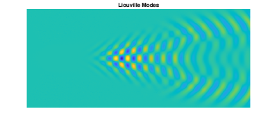
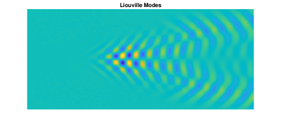
Refer to caption
Refer to caption
Refer to caption
Refer to caption
Refer to caption
Refer to caption
Refer to caption
Refer to caption
Refer to caption
Refer to caption
Refer to caption
Refer to caption
Figure 1: A selection of the real parts of approximate Liouville modes obtained using the exponential dot product kernel, where the domain corresponds to μ1=1/1000subscript𝜇111000\mu_{1}=1/1000 and the range corresponds to μ2=1/999subscript𝜇21999\mu_{2}=1/999.
Refer to caption
Refer to caption
Refer to caption
Refer to caption
Refer to caption
Refer to caption
Refer to caption
Refer to caption
Figure 2: A selection of reconstructed snapshots for the cyllinder flow example. The first column from the top presents snapshots 111, 212121, 414141, and 616161, and the second column presents 818181, 101101101, 121121121, and 141141141.
Refer to caption
Refer to caption
Refer to caption
Refer to caption
Refer to caption
Refer to caption
Refer to caption
Refer to caption
Figure 3: The original snapshots from the cyllinder flow data set in [11]. The first column from the top presents snapshots 111, 212121, 414141, and 616161, and the second column presents 818181, 101101101, 121121121, and 141141141.

10 Discussion

The methods presented in this manuscript give two algorithms for performing a dynamic mode decomposition. Together with the compactness of the Liouville operators, the singular DMD approach guarantees the existence of dynamic modes and convergence through singular value decomposition of compact operators. Singular DMD is a general purpose approach to performing a dynamic mode decomposition for when the domain and range of the operators disagree. The major drawback of this approach is that even though it can guarantee the existence of dynamic modes, which cannot be done for eigenfunction methods, the reconstruction involves the solution of an initial value problem, which is technically more involved than the eigenfunction approach.

The second method adds an additional assumption to the problem, where the domain is assumed to be embedded in the range of the operator. These embeddings frequently occur in the study of RKHSs, where the adjustment of a parameter loosens the requirement on functions within that space. It was demonstrated that this embedding may be established for the exponential dot product kernel, and it also holds for the native spaces of Gaussian RBFs with differing parameters.

Convergence of these routines follow the proof found in [16], which is a general purpose approach for showing convergence of operator level interpolants to the compact operators they are approximating. In particular, given an infinite collection of trajectories for a dynamical system, if the span of the occupation kernels form a dense subset of their respective Hilbert spaces, convergence of the overall algorithm is achieved.

The density of the occupation kernels corresponding to trajectories are easily established for Lipschitz continuous dynamics. This follows since, given any initial point, x0subscript𝑥0x_{0} in nsuperscript𝑛\mathbb{R}^{n}, there is a T0subscript𝑇0T_{0} such that the trajectory starting at x0subscript𝑥0x_{0}, γx0subscript𝛾subscript𝑥0\gamma_{x_{0}}, exists over the interval [0,T0]0subscript𝑇0[0,T_{0}]. Consider the sequence of occupation kernels indexed by δ[0,T0]𝛿0subscript𝑇0\delta\in[0,T_{0}], Γγx0,δ(x):=0δK(x,γx0(t))𝑑tassignsubscriptΓsubscript𝛾subscript𝑥0𝛿𝑥superscriptsubscript0𝛿𝐾𝑥subscript𝛾subscript𝑥0𝑡differential-d𝑡\Gamma_{\gamma_{x_{0}},\delta}(x):=\int_{0}^{\delta}K(x,\gamma_{x_{0}}(t))dt. Then 1δΓγx0,δK(x,x0)1𝛿subscriptΓsubscript𝛾subscript𝑥0𝛿𝐾𝑥subscript𝑥0\frac{1}{\delta}\Gamma_{\gamma_{x_{0}},\delta}\to K(x,x_{0}) in the Hilbert space norm. Hence, as x0subscript𝑥0x_{0} was arbitrary, every kernel may be approximated by an occupation kernel corresponding to a trajectory, and since kernels are dense in H𝐻H, so are these occupation kernels. Finally, if H𝐻H and H~~𝐻\tilde{H} are spaces of real analytic functions, the dynamics must also be real analytic by the same proof found in [17]. Spaces of real analytic functions include the Gaussian RBF and the exponential dot product kernel space.

One interesting result of the structure of the finite rank approximation given in Section 7 is that as μ1μ2subscript𝜇1subscript𝜇2\mu_{1}\to\mu_{2}, the first two matrices cancel. The matrix computations then approach the computations in [16]. Hence, for close enough μ1subscript𝜇1\mu_{1} and μ2subscript𝜇2\mu_{2} the computations are computationally indistinguishable from [16] over a fixed compact set containing the trajectories.

Finally, it should be noted that this methodology is not restricted to spaces of analytic functions, but rather it can work for a large collection of pairs of spaces. As a rule, the range space should be less restrictive as to the collection of functions in that space than the domain space. With this in mind, for many of the cases where compact Liouville operators may be established, the domain will embed into the range. The complications arise in computing the first matrix in (3), where the inner product of the occupation kernels for the domain are computed in the range space. Hence, the explicit description for spaces of real analytic functions help resolve that computation.

11 Conclusion

This manuscript presented a theoretical and algorithmic framework that achieves many long standing goals of dynamic mode decompositions. To wit, by selecting differing domains and ranges for the Liouville operators (sometimes Koopman generators), the resulting operators are compact. This comes at the sacrifice of eigenfunctions when the domain is not embedded in the range of the operator, but achieves well defined dynamic modes and convergence. Reconstruction can then be determined using typical numerical methods for initial value problems. However, in the case of an embedding between the spaces, an algorithm may be established to determine approximate eigenfunctions for the operators, resulting in a more typical DMD routine that also converges.

References

  • [1] N. Aronszajn, Theory of reproducing kernels, Transactions of the American mathematical society, 68 (1950), pp. 337–404.
  • [2] C. Bénéteau, M. C. Fleeman, D. S. Khavinson, D. Seco, and A. A. Sola, Remarks on inner functions and optimal approximants, Canadian mathematical bulletin, 61 (2018), pp. 704–716.
  • [3] S. L. Brunton and J. N. Kutz, Data-driven science and engineering: Machine learning, dynamical systems, and control, Cambridge University Press, 2019.
  • [4] M. Budišić, R. Mohr, and I. Mezić, Applied koopmanism, Chaos: An Interdisciplinary Journal of Nonlinear Science, 22 (2012), p. 047510.
  • [5] B. Carswell, B. D. MacCluer, and A. Schuster, Composition operators on the fock space, Acta Sci. Math.(Szeged), 69 (2003), pp. 871–887.
  • [6] G. Chacón and J. Giménez, Composition operators on spaces of entire functions, Proceedings of the American Mathematical Society, 135 (2007), pp. 2205–2218.
  • [7] S. Das, D. Giannakis, and J. Slawinska, Reproducing kernel hilbert space compactification of unitary evolution groups, Applied and Computational Harmonic Analysis, 54 (2021), pp. 75–136.
  • [8] E. Gonzalez, M. Abudia, M. Jury, R. Kamalapurkar, and J. A. Rosenfeld, Anti-Koopmanism, arXiv preprint arXiv:2106.00106, (2021).
  • [9] H. Hedenmalm, B. Korenblum, and K. Zhu, Theory of Bergman spaces, vol. 199, Springer Science & Business Media, 2012.
  • [10] M. Korda and I. Mezić, On convergence of extended dynamic mode decomposition to the Koopman operator, Journal of Nonlinear Science, 28 (2018), pp. 687–710.
  • [11] J. N. Kutz, S. L. Brunton, B. W. Brunton, and J. L. Proctor, Dynamic mode decomposition: data-driven modeling of complex systems, SIAM, 2016.
  • [12] A. Mauroy and I. Mezić, Global stability analysis using the eigenfunctions of the koopman operator, IEEE Transactions on Automatic Control, 61 (2016), pp. 3356–3369.
  • [13] I. Mezić, Spectral properties of dynamical systems, model reduction and decompositions, Nonlinear Dynamics, 41 (2005), pp. 309–325.
  • [14] G. K. Pedersen, Analysis now, vol. 118, Springer Science & Business Media, 2012.
  • [15] F. Riesz, Über die randwerte einer analytischen funktion, Mathematische Zeitschrift, 18 (1923), pp. 87–95.
  • [16] J. A. Rosenfeld, R. Kamalapurkar, L. F. Gruss, and T. T. Johnson, Dynamic mode decomposition for continuous time systems with the Liouville operator. arXiv:1910.03977, 2019.
  • [17] J. A. Rosenfeld, R. Kamalapurkar, B. Russo, and T. T. Johnson, Occupation kernels and densely defined Liouville operators for system identification, in IEEE Conference on Decision and Control, IEEE, 2019, pp. 6455–6460.
  • [18] I. Steinwart and A. Christmann, Support vector machines, Springer Science & Business Media, 2008.
  • [19] K. Zhu, Analysis on Fock spaces, vol. 263, Springer Science & Business Media, 2012.