Sigma-Delta and Distributed Noise-Shaping Quantization Methods for Random Fourier Features

Jinjie Zhang Department of Mathematics, University of California San Diego jiz003@ucsd.edu Harish Kannan Department of Mathematics, University of California San Diego hkannan@ucsd.edu Alexander Cloninger Department of Mathematics and Halıcıoğlu Data Science Institute, University of California San Diego acloninger@ucsd.edu  and  Rayan Saab Department of Mathematics and Halıcıoğlu Data Science Institute, University of California San Diego rsaab@ucsd.edu
Abstract.

We propose the use of low bit-depth Sigma-Delta and distributed noise-shaping methods for quantizing the Random Fourier features (RFFs) associated with shift-invariant kernels. We prove that our quantized RFFs – even in the case of 111-bit quantization – allow a high accuracy approximation of the underlying kernels, and the approximation error decays at least polynomially fast as the dimension of the RFFs increases. We also show that the quantized RFFs can be further compressed, yielding an excellent trade-off between memory use and accuracy. Namely, the approximation error now decays exponentially as a function of the bits used. Moreover, we empirically show by testing the performance of our methods on several machine learning tasks that our method compares favorably to other state of the art quantization methods in this context.

1. Introduction

Kernel methods have long been demonstrated as effective techniques in various machine learning applications, cf. [33, 32]. Given a dataset 𝒳d𝒳superscript𝑑\mathcal{X}\subset\mathbb{R}^{d} with |𝒳|=N𝒳𝑁|\mathcal{X}|=N, kernel methods implicitly map data points to a high, possibly infinite, dimensional feature space \mathcal{H} by ϕ:𝒳:italic-ϕ𝒳\phi:\mathcal{X}\rightarrow\mathcal{H}. However, instead of working directly on that space the inner products between feature embeddings can be preserved by a kernel function k(x,y):=ϕ(x),ϕ(y)assign𝑘𝑥𝑦subscriptitalic-ϕ𝑥italic-ϕ𝑦k(x,y):=\langle\phi(x),\phi(y)\rangle_{\mathcal{H}} that coincides with the inner product. Nevertheless, in cases where N𝑁N is large, using nonlinear kernels for applications like, say, support vector machines (SVM) and logistic regression requires the expensive computation of the N×N𝑁𝑁N\times N Gram matrix of the data [24]. In order to overcome this bottleneck, one popular approach is to “linearize” k𝑘k by using the random Fourier features (RFFs) originally proposed by [29], and in turn built on Bochner’s theorem [26]. Given a continuous, shift-invariant real-valued kernel k(x,y)=κ(xy)𝑘𝑥𝑦𝜅𝑥𝑦k(x,y)=\kappa(x-y) with κ(0)=1𝜅01\kappa(0)=1, then κ𝜅\kappa is the (inverse) Fourier transform of a probability measure ΛΛ\Lambda over dsuperscript𝑑\mathbb{R}^{d} and we have

(1) κ(u)=𝔼ωΛexp(iωu)=𝔼ωΛcos(ωu).𝜅𝑢subscript𝔼similar-to𝜔Λ𝑖superscript𝜔top𝑢subscript𝔼similar-to𝜔Λsuperscript𝜔top𝑢\kappa(u)=\mathbb{E}_{\omega\sim\Lambda}\exp(i\omega^{\top}u)=\mathbb{E}_{\omega\sim\Lambda}\cos(\omega^{\top}u).

As an example, the radial basis function (RBF) kernel k(x,y)=exp(xy22/2σ2)𝑘𝑥𝑦superscriptsubscriptnorm𝑥𝑦222superscript𝜎2k(x,y)=\exp(-\|x-y\|_{2}^{2}/2\sigma^{2}) corresponds to the multivariate normal distribution Λ=𝒩(0,σ2Id)Λ𝒩0superscript𝜎2subscript𝐼𝑑\Lambda=\mathcal{N}(0,\sigma^{-2}I_{d}). Following [29], for a target dimension m𝑚m, the associated RFFs (without normalization) are

(2) z(x):=cos(Ωx+ξ)massign𝑧𝑥superscriptΩtop𝑥𝜉superscript𝑚z(x):=\cos(\Omega^{\top}x+\xi)\in\mathbb{R}^{m}

where Ω:=(ω1,,ωm)d×massignΩsubscript𝜔1subscript𝜔𝑚superscript𝑑𝑚\Omega:=(\omega_{1},\ldots,\omega_{m})\in\mathbb{R}^{d\times m} is a random matrix generated as ωjiidΛsubscript𝜔𝑗𝑖𝑖𝑑similar-toΛ\omega_{j}\overset{iid}{\sim}\Lambda and ξm𝜉superscript𝑚\xi\in\mathbb{R}^{m} is a random vector with ξjiidU([0,2π))subscript𝜉𝑗𝑖𝑖𝑑similar-to𝑈02𝜋\xi_{j}\overset{iid}{\sim}U([0,2\pi)) for all j𝑗j. Additionally, the identity 𝔼(z(x),z(y))=m2k(x,y)𝔼𝑧𝑥𝑧𝑦𝑚2𝑘𝑥𝑦\mathbb{E}(\langle z(x),z(y)\rangle)=\frac{m}{2}k(x,y) implies that the inner product of low-dimensional features 2mz(x)2𝑚𝑧𝑥\sqrt{\frac{2}{m}}z(x), 2mz(y)2𝑚𝑧𝑦\sqrt{\frac{2}{m}}z(y) can approximate k(x,y)𝑘𝑥𝑦k(x,y) in kernel-based algorithms. Learning a linear model on the (normalized) RFFs then amounts to using the approximation

(3) k^RFF(x,y):=2mz(x),z(y)assignsubscript^𝑘RFF𝑥𝑦2𝑚𝑧𝑥𝑧𝑦\widehat{k}_{\text{RFF}}(x,y):=\frac{2}{m}\langle z(x),z(y)\rangle

as a reference kernel during training. For instance, performing linear SVM and linear ridge regression on RFFs winds up training nonlinear kernel-based SVM and ridge regression with k^RFFsubscript^𝑘RFF\widehat{k}_{\text{RFF}}. It turns out that using RFFs in such a way with adjustable dimension m𝑚m can remarkably speed up training for large-scale data and alleviate the memory burden for storing the kernel matrix. As an additional and very important benefit, the entire kernel function k𝑘k is approximated accurately, i.e., the approximation error |k(x,y)k^RFF(x,y)|𝑘𝑥𝑦subscript^𝑘RFF𝑥𝑦|k(x,y)-\widehat{k}_{\text{RFF}}(x,y)| has been shown to be small, particularly when m𝑚m is large, e.g., in [30, 5, 37, 34, 3, 4].

The need for large m𝑚m for guaranteeing good generalization performance on large datasets [38, 27, 1, 25] provides an opportunity for further savings in memory usage. Rather than store the RFFs in full precision, quantization methods have been proposed to encode RFFs (2) into a sequence of bits and subsequently approximate k(x,y)𝑘𝑥𝑦k(x,y) by taking inner product between quantized RFFs, thereby introducing a new level of approximation. One of our goals is to propose quantization techniques that favorably trade off approximation accuracy against number of bits used.

1.1. Related Work

To make the discussion more precise, let us start by defining the 2K2𝐾2K-level quantization alphabet that we use throughout as

(4) 𝒜={a2K1|a=±1,±3,,±(2K1)},𝒜conditional-set𝑎2𝐾1𝑎plus-or-minus1plus-or-minus3plus-or-minus2𝐾1\mathcal{A}=\Bigl{\{}\frac{a}{2K-1}\,\Big{|}\,a=\pm 1,\pm 3,\ldots,\pm(2K-1)\Bigr{\}},

and note that one can use b:=log2(2K)assign𝑏subscript22𝐾b:=\log_{2}(2K) bits to represent each element of 𝒜𝒜\mathcal{A}. The goal of quantization in the RFF context is to map z(x)=cos(ΩTx+ξ)mq(x)𝒜m𝑧𝑥superscriptΩ𝑇𝑥𝜉superscript𝑚maps-to𝑞𝑥superscript𝒜𝑚z(x)=\cos(\Omega^{T}x+\xi)\in\mathbb{R}^{m}\mapsto q(x)\in\mathcal{A}^{m}. We will be interested in very small values of K𝐾K, particularly K=1𝐾1K=1, which corresponds to very few bits per RFF sample.

It is natural to start our discussion of quantization methods with the simplest quantizer, namely memoryless scalar quantization (MSQ), where we round each coordinate of the input vector zm𝑧superscript𝑚z\in\mathbb{R}^{m} to the nearest element in 𝒜𝒜\mathcal{A}. Specifically, QMSQ:m𝒜m:subscript𝑄MSQsuperscript𝑚superscript𝒜𝑚Q_{\mathrm{MSQ}}:\mathbb{R}^{m}\rightarrow\mathcal{A}^{m} is defined by

qi:=(QMSQ(z))i:=argminv𝒜|ziv|,i=1,,m.formulae-sequenceassignsubscript𝑞𝑖subscriptsubscript𝑄MSQ𝑧𝑖assignsubscriptargmin𝑣𝒜subscript𝑧𝑖𝑣𝑖1𝑚q_{i}:=(Q_{\mathrm{MSQ}}(z))_{i}:=\operatorname{argmin}_{v\in\mathcal{A}}|z_{i}-v|,\quad i=1,\ldots,m.

Moreover, by setting K=1𝐾1K=1, one can get a binary embedding QMSQ(z)=sign(z)subscript𝑄MSQ𝑧sign𝑧Q_{\mathrm{MSQ}}(z)=\operatorname{sign}(z) with 𝒜={1,1}𝒜11\mathcal{A}=\{-1,1\} where signsign\operatorname{sign} is an element-wise operation. This yields the so-called one-bit universal quantizer [8, 31] for RFFs, which generates a distorted (biased) kernel

(5) k^q(x,y):=1msign(z(x)),sign(z(y)).assignsubscript^𝑘𝑞𝑥𝑦1𝑚sign𝑧𝑥sign𝑧𝑦\widehat{k}_{q}(x,y):=\frac{1}{m}\langle\operatorname{sign}(z(x)),\operatorname{sign}(z(y))\rangle.

Although replacing the signsign\operatorname{sign} function in (5) by QMSQsubscript𝑄𝑀𝑆𝑄Q_{MSQ} with K>1𝐾1K>1 and renormalizing the inner product correspondingly can alleviate the distortion, there are better choices in terms of approximation error. In [23], a Lloyd-Max (LM) quantization scheme is designed based on the MSQ where, rather than use the evenly spaced alphabet in (4), one has to construct specific alphabets for different K𝐾K. Recently with an eye towards asymmetric sensor network applications, an asymmetric semi-quantized scheme (SemiQ) was proposed in [31], and shown to be unbiased. It generates k^s(x,y)subscript^𝑘𝑠𝑥𝑦\widehat{k}_{s}(x,y), which is an inner product between an unquantized RFF vector and a quantized one, i.e.

(6) k^s(x,y):=π2mz(x),QMSQ(z(y)).assignsubscript^𝑘𝑠𝑥𝑦𝜋2𝑚𝑧𝑥subscript𝑄MSQ𝑧𝑦\widehat{k}_{s}(x,y):=\frac{\pi}{2m}\langle z(x),Q_{\mathrm{MSQ}}(z(y))\rangle.

However, this asymmetric setting is restrictive on many kernel machines because it only works for the inference stage and the model still has to be trained based on unquantized RFFs. Another unbiased quantization scheme resorts to injecting randomness into the quantization, and is known as randomized rounding [41], or stochastic quantization (StocQ) [23]. Specifically, for each z𝑧z\in\mathbb{R}, one chooses the two consecutive points s,t𝒜𝑠𝑡𝒜s,t\in\mathcal{A} with z[s,t]𝑧𝑠𝑡z\in[s,t]. Then one randomly assigns the quantization via P(QStocQ(z)=s)=tztsPsubscript𝑄StocQ𝑧𝑠𝑡𝑧𝑡𝑠\mathrm{P}(Q_{\mathrm{StocQ}}(z)=s)=\frac{t-z}{t-s}, P(QStocQ(z)=t)=zstsPsubscript𝑄StocQ𝑧𝑡𝑧𝑠𝑡𝑠\mathrm{P}(Q_{\mathrm{StocQ}}(z)=t)=\frac{z-s}{t-s}. It follows that

(7) k^StocQ(x,y):=2mQStocQ(z(x)),QStocQ(z(y))assignsubscript^𝑘StocQ𝑥𝑦2𝑚subscript𝑄StocQ𝑧𝑥subscript𝑄StocQ𝑧𝑦\widehat{k}_{\mathrm{StocQ}}(x,y):=\frac{2}{m}\langle Q_{\mathrm{StocQ}}(z(x)),Q_{\mathrm{StocQ}}(z(y))\rangle

where QStocQsubscript𝑄StocQQ_{\mathrm{StocQ}} operates on each component separately. Due to the Bernoulli sampling for QStocQsubscript𝑄StocQQ_{\mathrm{StocQ}}, the quantization process involves additional randomness for each dimension of RFFs, which leads to extra variance especially in the case of binary embedding, i.e., b=1𝑏1b=1. Nevertheless, the kernel approximation error for k^ssubscript^𝑘𝑠\widehat{k}_{s} and k^StocQsubscript^𝑘StocQ\widehat{k}_{\text{StocQ}} is bounded by O(m1/2)𝑂superscript𝑚12O(m^{-1/2}) with high probability, see [31, 41].

1.2. Methods and Contributions

We explore the use of ΣΔΣΔ\Sigma\Delta [14, 15, 18] and distributed noise-shaping [9, 10] quantization methods on RFFs. These techniques, explicitly defined and discussed in Section 2 and Appendix A, yield superior performance to methods based on scalar quantization in contexts ranging from bandlimited function quantization [14, 18], to quantization of linear measurements [7, 6], of compressed sensing measurements [19], of non-linear measurements [20], and even for binary embeddings that preserve (Euclidean) distances [21, 40]. It is therefore natural to wonder whether they can also yield superior performance in the RFF context. Let QΣΔ(r)superscriptsubscript𝑄ΣΔ𝑟Q_{\Sigma\Delta}^{(r)} be the r𝑟r-th order ΣΔΣΔ\Sigma\Delta quantizer and let Qβsubscript𝑄𝛽Q_{\beta} be the distributed noise shaping quantizer with β(1,2)𝛽12\beta\in(1,2), and let V~ΣΔsubscript~𝑉ΣΔ\widetilde{V}_{\Sigma\Delta} and V~βsubscript~𝑉𝛽\widetilde{V}_{\beta} be their associated sparse condensation matrices defined in Section 2. Then our method approximates kernels via

(8) k^ΣΔ(r)(x,y):=V~ΣΔQΣΔ(r)(z(x)),V~ΣΔQΣΔ(r)(z(y))assignsubscriptsuperscript^𝑘𝑟ΣΔ𝑥𝑦subscript~𝑉ΣΔsuperscriptsubscript𝑄ΣΔ𝑟𝑧𝑥subscript~𝑉ΣΔsuperscriptsubscript𝑄ΣΔ𝑟𝑧𝑦\widehat{k}^{(r)}_{\Sigma\Delta}(x,y):=\langle\widetilde{V}_{\Sigma\Delta}Q_{\Sigma\Delta}^{(r)}(z(x)),\widetilde{V}_{\Sigma\Delta}Q_{\Sigma\Delta}^{(r)}(z(y))\rangle

and

(9) k^β(x,y):=V~βQβ(z(x)),V~βQβ(z(y)).assignsubscript^𝑘𝛽𝑥𝑦subscript~𝑉𝛽subscript𝑄𝛽𝑧𝑥subscript~𝑉𝛽subscript𝑄𝛽𝑧𝑦\widehat{k}_{\beta}(x,y):=\langle\widetilde{V}_{\beta}Q_{\beta}(z(x)),\widetilde{V}_{\beta}Q_{\beta}(z(y))\rangle.

Specifically, given large-scale data 𝒯𝒯\mathcal{T} contained in a compact set 𝒳d𝒳superscript𝑑\mathcal{X}\subset\mathbb{R}^{d}, we put forward Algorithm 1 to generate and store quantized RFFs such that one can subsequently use them for training and inference using linear models.

Input: Shift-invariant kernel k𝑘k, alphabet 𝒜𝒜\mathcal{A}, and training data 𝒯={xi}i=1N𝒳𝒯superscriptsubscriptsubscript𝑥𝑖𝑖1𝑁𝒳\mathcal{T}=\{x_{i}\}_{i=1}^{N}\subset\mathcal{X}
1 Generate random matrix Ωd×mΩsuperscript𝑑𝑚\Omega\in\mathbb{R}^{d\times m} and random vector ξm𝜉superscript𝑚\xi\in\mathbb{R}^{m} as in (2)
2 for i=1𝑖1i=1 to N𝑁N do
3       zicos(Ωxi+ξ)msubscript𝑧𝑖superscriptΩtopsubscript𝑥𝑖𝜉superscript𝑚z_{i}\leftarrow\cos(\Omega^{\top}x_{i}+\xi)\in\mathbb{R}^{m} \triangleright Compute RFFs
4       qiQ(zi)𝒜msubscript𝑞𝑖𝑄subscript𝑧𝑖superscript𝒜𝑚q_{i}\leftarrow Q(z_{i})\in\mathcal{A}^{m} \triangleright Q=QΣΔ(r)𝑄superscriptsubscript𝑄ΣΔ𝑟Q=Q_{\Sigma\Delta}^{(r)} or Qβsubscript𝑄𝛽Q_{\beta} as in (10) and (13)
5       yiV~qisubscript𝑦𝑖~𝑉subscript𝑞𝑖y_{i}\leftarrow\widetilde{V}q_{i} \triangleright Further compression with V~=V~ΣΔ~𝑉subscript~𝑉ΣΔ\widetilde{V}=\widetilde{V}_{\Sigma\Delta} or V~βsubscript~𝑉𝛽\widetilde{V}_{\beta} as in (14)
Store {yi}i=1Nsuperscriptsubscriptsubscript𝑦𝑖𝑖1𝑁\{y_{i}\}_{i=1}^{N} and use it to train kernel machines with a linear kernel, i.e. inner product
Algorithm 1 Quantized kernel machines

For illustration, Appendix B presents a pointwise comparison of above kernel approximations on a synthetic toy dataset. A summary of our contributions follows.

  • We give the first detailed analysis of ΣΔΣΔ\Sigma\Delta and distributed noise-shaping schemes for quantizing RFFs. Specifically, Theorem 3.1 provides a uniform upper bound for the errors |k^ΣΔ(r)(x,y)k(x,y)|subscriptsuperscript^𝑘𝑟ΣΔ𝑥𝑦𝑘𝑥𝑦|\widehat{k}^{(r)}_{\Sigma\Delta}(x,y)-k(x,y)| and |k^β(x,y)k(x,y)|subscript^𝑘𝛽𝑥𝑦𝑘𝑥𝑦|\widehat{k}_{\beta}(x,y)-k(x,y)| over compact (possibly infinite) sets. Our analysis shows that the quantization error decays fast as m𝑚m grows. Additionally, Theorem 3.3 provides spectral approximation guarantees for first order ΣΔΣΔ\Sigma\Delta quantized RFF approximation of kernels.

  • Our methods allow a further reduction in the number of bits used. Indeed, to implement (8) and (9) in practice, one would store and transmit the condensed bitstreams V~ΣΔQΣΔ(r)(z(x))subscript~𝑉ΣΔsuperscriptsubscript𝑄ΣΔ𝑟𝑧𝑥\widetilde{V}_{\Sigma\Delta}Q_{\Sigma\Delta}^{(r)}(z(x)) or V~βQβ(z(x))subscript~𝑉𝛽subscript𝑄𝛽𝑧𝑥\widetilde{V}_{\beta}Q_{\beta}(z(x)). For example, since the matrices V~ΣΔsubscript~𝑉ΣΔ\widetilde{V}_{\Sigma\Delta} are sparse and essentially populated by bounded integers, each sample can be represented by fewer bits, as summarized in Table 1.

  • We illustrate the benefits of our proposed methods in several numerical experiments involving kernel ridge regression (KRR), kernel SVM, and two-sample tests based on maximum mean discrepancy (MMD) (all in Section 4). Our experiments show that QΣΔ(r)superscriptsubscript𝑄ΣΔ𝑟Q_{\Sigma\Delta}^{(r)} and Qβsubscript𝑄𝛽Q_{\beta} are comparable with the semi-quantization scheme and outperforms the other fully-quantized method mentioned above, both when we fix the number of RFF features m𝑚m, and when we fix the number of bits used to store each quantized RFF vector.

2. Noise Shaping Quantization Preliminaries

The methods we consider herein are special cases of noise shaping quantization schemes (see, e.g., [11]). For a fixed alphabet 𝒜𝒜\mathcal{A} and each dimension m𝑚m, such schemes are associated with an m×m𝑚𝑚m\times m lower triangular matrix H𝐻H with unit diagonal, and are given by a map Q:m𝒜m:𝑄superscript𝑚superscript𝒜𝑚Q:\mathbb{R}^{m}\to\mathcal{A}^{m} with yqmaps-to𝑦𝑞y\mapsto q designed to satisfy yq=Hu𝑦𝑞𝐻𝑢y-q=Hu. The schemes are called stable if uCsubscriptnorm𝑢𝐶\|u\|_{\infty}\leq C where C𝐶C is independent of m𝑚m. Among these noise shaping schemes, we will be interested in stable rthsuperscript𝑟thr^{\text{th}} order ΣΔΣΔ\Sigma\Delta schemes QΣΔ(r)superscriptsubscript𝑄ΣΔ𝑟Q_{\Sigma\Delta}^{(r)} [18, 15], and distributed noise shaping schemes Qβsubscript𝑄𝛽Q_{\beta} [9, 10]. For example, in the case of ΣΔΣΔ\Sigma\Delta with r=1𝑟1r=1, the entries qi,i=1,,mformulae-sequencesubscript𝑞𝑖𝑖1𝑚q_{i},i=1,...,m of the vector q=QΣΔ(1)(y)𝑞superscriptsubscript𝑄ΣΔ1𝑦q=Q_{\Sigma\Delta}^{(1)}(y) are assigned iteratively via

(10) {u0=0,qi=QMSQ(yi+ui1),ui=ui1+yiqi,casessubscript𝑢00otherwisesubscript𝑞𝑖subscript𝑄MSQsubscript𝑦𝑖subscript𝑢𝑖1otherwisesubscript𝑢𝑖subscript𝑢𝑖1subscript𝑦𝑖subscript𝑞𝑖otherwise\begin{cases}u_{0}=0,\\ q_{i}=Q_{\mathrm{MSQ}}\bigl{(}y_{i}+u_{i-1}\bigr{)},\\ u_{i}=u_{i-1}+y_{i}-q_{i},\end{cases}

where QMSQ(z)=argminv𝒜|zv|subscript𝑄MSQ𝑧subscriptargmin𝑣𝒜𝑧𝑣Q_{\mathrm{MSQ}}(z)=\operatorname{argmin}_{v\in\mathcal{A}}|z-v|. This yields the difference equation yq=Du𝑦𝑞𝐷𝑢y-q=Du where D𝐷D is the first order difference matrix given by Dij=1subscript𝐷𝑖𝑗1D_{ij}=1 if i=j𝑖𝑗i=j, Dij=1subscript𝐷𝑖𝑗1D_{ij}=-1 if i=j+1𝑖𝑗1i=j+1, and 00 otherwise. Stable ΣΔΣΔ\Sigma\Delta schemes with r>1𝑟1r>1, are more complicated to construct (see Appendix A), but satisfy

(11) Dru=yq.superscript𝐷𝑟𝑢𝑦𝑞D^{r}u=y-q.

On the other hand, a distributed noise-shaping quantizer Qβ:m𝒜m:subscript𝑄𝛽superscript𝑚superscript𝒜𝑚Q_{\beta}:\mathbb{R}^{m}\rightarrow\mathcal{A}^{m} converts the input vector ym𝑦superscript𝑚y\in\mathbb{R}^{m} to q=Qβ(y)𝒜m𝑞subscript𝑄𝛽𝑦superscript𝒜𝑚q=Q_{\beta}(y)\in\mathcal{A}^{m} such that

(12) Hu=yq𝐻𝑢𝑦𝑞Hu=y-q

where, again, uCsubscriptnorm𝑢𝐶\|u\|_{\infty}\leq C. Here, denoting the p×p𝑝𝑝p\times p identity matrix by Ipsubscript𝐼𝑝I_{p} and the Kronecker product by tensor-product\otimes, H𝐻H is a block diagonal matrix defined as H:=IpHβm×massign𝐻tensor-productsubscript𝐼𝑝subscript𝐻𝛽superscript𝑚𝑚H:=I_{p}\otimes H_{\beta}\in\mathbb{R}^{m\times m} where Hβλ×λsubscript𝐻𝛽superscript𝜆𝜆H_{\beta}\in\mathbb{R}^{\lambda\times\lambda} is given by (Hβ)ij=1subscriptsubscript𝐻𝛽𝑖𝑗1({H_{\beta}})_{ij}=1 if i=j𝑖𝑗i=j, (Hβ)ij=βsubscriptsubscript𝐻𝛽𝑖𝑗𝛽({H_{\beta}})_{ij}=-\beta if i=j+1𝑖𝑗1i=j+1, and 00 otherwise. Defining H~:=ImHassign~𝐻subscript𝐼𝑚𝐻\widetilde{H}:=I_{m}-H, one can implement the quantization step q=Qβ(y)𝑞subscript𝑄𝛽𝑦q=Q_{\beta}(y) via the following iterations for i=1,2,,m𝑖12𝑚i=1,2,\ldots,m [9, 10]:

(13) {u0=0,qi=QMSQ(yi+H~i,i1ui1),ui=yi+H~i,i1ui1qi,casessubscript𝑢00otherwisesubscript𝑞𝑖subscript𝑄MSQsubscript𝑦𝑖subscript~𝐻𝑖𝑖1subscript𝑢𝑖1otherwisesubscript𝑢𝑖subscript𝑦𝑖subscript~𝐻𝑖𝑖1subscript𝑢𝑖1subscript𝑞𝑖otherwise\begin{cases}u_{0}=0,\\ q_{i}=Q_{\mathrm{MSQ}}\bigl{(}y_{i}+\widetilde{H}_{i,i-1}u_{i-1}\bigr{)},\\ u_{i}=y_{i}+\widetilde{H}_{i,i-1}u_{i-1}-q_{i},\end{cases}

where QMSQ(z)=argminv𝒜|zv|subscript𝑄MSQ𝑧subscriptargmin𝑣𝒜𝑧𝑣Q_{\mathrm{MSQ}}(z)=\operatorname{argmin}_{v\in\mathcal{A}}|z-v|. The stability of (13) is discussed in Appendix A. It is worth mentioning that since QΣΔ(r)superscriptsubscript𝑄ΣΔ𝑟Q_{\Sigma\Delta}^{(r)} and Qβsubscript𝑄𝛽Q_{\beta} are sequential quantization methods, they can not be implemented entirely in parallel. On the other hand, blocks of size λ𝜆\lambda can still be run in parallel. Next, we adopt the definition of a condensation operator in [9, 21, 40].

Definition 2.1 (ΣΔΣΔ\Sigma\Delta condensation operator).

Let p𝑝p, r𝑟r, λ𝜆\lambda be fixed positive integers such that λ=rλ~r+1𝜆𝑟~𝜆𝑟1\lambda=r\widetilde{\lambda}-r+1 for some integer λ~~𝜆\widetilde{\lambda}. Let m=λp𝑚𝜆𝑝m=\lambda p and v𝑣v be a row vector in λsuperscript𝜆\mathbb{R}^{\lambda} whose entry vjsubscript𝑣𝑗v_{j} is the j𝑗j-th coefficient of the polynomial (1+z++zλ~1)rsuperscript1𝑧superscript𝑧~𝜆1𝑟(1+z+\ldots+z^{\widetilde{\lambda}-1})^{r}. Define the condensation operator VΣΔp×msubscript𝑉ΣΔsuperscript𝑝𝑚V_{\Sigma\Delta}\in\mathbb{R}^{p\times m} as VΣΔ:=Ipv.assignsubscript𝑉ΣΔtensor-productsubscript𝐼𝑝𝑣V_{\Sigma\Delta}:=I_{p}\otimes v.

For example, when r=1𝑟1r=1, λ=λ~𝜆~𝜆\lambda=\widetilde{\lambda} and the vector vλ𝑣superscript𝜆v\in\mathbb{R}^{\lambda} is simply the vector of all ones while when r=2𝑟2r=2, λ=2λ~1𝜆2~𝜆1\lambda=2\widetilde{\lambda}-1 and v=(1,2,,λ~1,λ~,λ~1,,2,1)λ𝑣12~𝜆1~𝜆~𝜆121superscript𝜆v=(1,2,\ldots,\widetilde{\lambda}-1,\widetilde{\lambda},\widetilde{\lambda}-1,\ldots,2,1)\in\mathbb{R}^{\lambda}.

Definition 2.2 (Distributed noise-shaping condensation operator).

Let p,λ𝑝𝜆p,\lambda be positive integers and fix β(1,2)𝛽12\beta\in(1,2). Let m=λp𝑚𝜆𝑝m=\lambda p and vβ:=(β1,β2,,βλ)λassignsubscript𝑣𝛽superscript𝛽1superscript𝛽2superscript𝛽𝜆superscript𝜆v_{\beta}:=(\beta^{-1},\beta^{-2},\ldots,\beta^{-\lambda})\in\mathbb{R}^{\lambda} be a row vector. Define the distributed noise-shaping condensation operator Vβp×msubscript𝑉𝛽superscript𝑝𝑚V_{\beta}\in\mathbb{R}^{p\times m} as Vβ:=Ipvβ.assignsubscript𝑉𝛽tensor-productsubscript𝐼𝑝subscript𝑣𝛽V_{\beta}:=I_{p}\otimes v_{\beta}.

We will also need the normalized condensation operators given by

(14) V~ΣΔ:=2pv2VΣΔ,V~β:=2pvβ2Vβ.formulae-sequenceassignsubscript~𝑉ΣΔ2𝑝subscriptnorm𝑣2subscript𝑉ΣΔassignsubscript~𝑉𝛽2𝑝subscriptnormsubscript𝑣𝛽2subscript𝑉𝛽\widetilde{V}_{\Sigma\Delta}:=\frac{\sqrt{2}}{\sqrt{p}\|v\|_{2}}V_{\Sigma\Delta},\qquad\widetilde{V}_{\beta}:=\frac{\sqrt{2}}{\sqrt{p}\|v_{\beta}\|_{2}}V_{\beta}.

If V~~𝑉\widetilde{V} is either of the two normalized matrices in (14), Lemma D.3 (Appendix D) shows that

(15) 𝔼(V~z(x),V~z(y))=k(x,y).𝔼~𝑉𝑧𝑥~𝑉𝑧𝑦𝑘𝑥𝑦\mathbb{E}(\langle\widetilde{V}z(x),\widetilde{V}z(y)\rangle)=k(x,y).

3. Main Results and Space Complexity

Our approach to quantizing RFFs given by (8) and (9) is justified by (15), along with the observation that, for our noise-shaping schemes, we have q=zHu𝑞𝑧𝐻𝑢q=z-Hu with guarantees that V~Hu2subscriptnorm~𝑉𝐻𝑢2\|\widetilde{V}Hu\|_{2} is small.

Moreover, as we will see in Section 3.1, we are able to control the approximation error such that k^ΣΔ(x,y)k(x,y)subscript^𝑘ΣΔ𝑥𝑦𝑘𝑥𝑦\widehat{k}_{\Sigma\Delta}(x,y)\approx k(x,y) and k^β(x,y)k(x,y)subscript^𝑘𝛽𝑥𝑦𝑘𝑥𝑦\widehat{k}_{\beta}(x,y)\approx k(x,y) hold with high probability. In fact Theorem 3.1 shows more: the approximation error of the quantized kernel estimators in (8) and (9) have polynomial and exponential error decay respectively as a function of m𝑚m, the dimension of the RFFs. Armed with this result, in Section 3.2 we also present a brief analysis of the space-complexity associated with our quantized RFFs, and show that the approximation error due to quantization decays exponentially as a function of the bits needed.

Additionally, in various applications such as Kernel Ridge Regression (KRR), spectral error bounds on the kernel may be more pertinent than point-wise bounds. For example, it was shown in [4, 41] that the expected loss of kernel ridge regression performed using an approximation of the true kernel is bounded by a function of the spectral error in the kernel approximation (Lemma 2 of [4], Proposition 1 of [41]). In Theorem 3.3, we provide spectral approximation guarantees for first order ΣΔΣΔ\Sigma\Delta quantized RFF approximation of kernels, in the spirit of the analogous guarantees in [41] for stochastic quantization.

3.1. Approximation error bounds

3.1.1. Point-wise error bounds on the approximation

We begin with Theorem 3.1, with its proof in Appendix D.

Theorem 3.1.

Let 𝒳d𝒳superscript𝑑\mathcal{X}\subseteq\mathbb{R}^{d} be compact with diameter >00\ell>0 and k:𝒳×𝒳:𝑘𝒳𝒳k:\mathcal{X}\times\mathcal{X}\rightarrow\mathbb{R} be a normalized, i.e. k(0,0)=1𝑘001k(0,0)=1, shift-invariant kernel. Let ΛΛ\Lambda be its corresponding probability measure as in (1), and suppose that the second moment σΛ2=𝔼ωΛω22superscriptsubscript𝜎Λ2subscript𝔼similar-to𝜔Λsuperscriptsubscriptnorm𝜔22\sigma_{\Lambda}^{2}=\mathbb{E}_{\omega\sim\Lambda}\|\omega\|_{2}^{2} exists. Let β(1,2)𝛽12\beta\in(1,2), p,r𝑝𝑟p,r\in\mathbb{N}, λ=O(plog1p)𝜆𝑂𝑝superscript1𝑝\lambda=O(\sqrt{p\log^{-1}p})\in\mathbb{N}, and m=λp𝑚𝜆𝑝m=\lambda p. For x,y𝒳𝑥𝑦𝒳x,y\in\mathcal{X}, and b𝑏b-bit alphabet 𝒜𝒜\mathcal{A} in (4) with b=log2(2K)𝑏subscript22𝐾b=\log_{2}(2K), consider the approximated kernels k^ΣΔ(r)(x,y)subscriptsuperscript^𝑘𝑟ΣΔ𝑥𝑦\widehat{k}^{(r)}_{\Sigma\Delta}(x,y) and k^β(x,y)subscript^𝑘𝛽𝑥𝑦\widehat{k}_{\beta}(x,y) defined as in (8) and (9) respectively. Then there exist positive constants {αi}i=110superscriptsubscriptsubscript𝛼𝑖𝑖110\{\alpha_{i}\}_{i=1}^{10} that are independent of m,p,λ𝑚𝑝𝜆m,p,\lambda such that

(16) supx,y𝒳|k^ΣΔ(r)(x,y)k(x,y)|(logpp)1/2+log1/2pλr1(2b1)+1λ2r1(2b1)2less-than-or-similar-tosubscriptsupremum𝑥𝑦𝒳superscriptsubscript^𝑘ΣΔ𝑟𝑥𝑦𝑘𝑥𝑦superscript𝑝𝑝12superscript12𝑝superscript𝜆𝑟1superscript2𝑏11superscript𝜆2𝑟1superscriptsuperscript2𝑏12\sup_{x,y\in\mathcal{X}}\bigl{|}\widehat{k}_{\Sigma\Delta}^{(r)}(x,y)-k(x,y)\bigr{|}\lesssim\Bigl{(}\frac{\log p}{p}\Bigr{)}^{1/2}+\frac{\log^{1/2}p}{\lambda^{r-1}(2^{b}-1)}+\frac{1}{\lambda^{2r-1}(2^{b}-1)^{2}}

holds with probability at least 1α1p1α2α3exp(α4p1/2+α5logp)1subscript𝛼1superscript𝑝1subscript𝛼2subscript𝛼3subscript𝛼4superscript𝑝12subscript𝛼5𝑝1-\alpha_{1}p^{-1-\alpha_{2}}-\alpha_{3}\exp(-\alpha_{4}p^{1/2}+\alpha_{5}\log p), and

(17) supx,y𝒳|k^β(x,y)k(x,y)|(logpp)1/2+p1/2βλ1(2b1)+1β2λ2(2b1)2less-than-or-similar-tosubscriptsupremum𝑥𝑦𝒳subscript^𝑘𝛽𝑥𝑦𝑘𝑥𝑦superscript𝑝𝑝12superscript𝑝12superscript𝛽𝜆1superscript2𝑏11superscript𝛽2𝜆2superscriptsuperscript2𝑏12\sup_{x,y\in\mathcal{X}}\bigl{|}\widehat{k}_{\beta}(x,y)-k(x,y)\bigr{|}\lesssim\Bigl{(}\frac{\log p}{p}\Bigr{)}^{1/2}+\frac{p^{1/2}}{\beta^{\lambda-1}(2^{b}-1)}+\frac{1}{\beta^{2\lambda-2}(2^{b}-1)^{2}}

holds with probability exceeding 1α6p1α7α8exp(α9p1/2+α10logp)1subscript𝛼6superscript𝑝1subscript𝛼7subscript𝛼8subscript𝛼9superscript𝑝12subscript𝛼10𝑝1-\alpha_{6}p^{-1-\alpha_{7}}-\alpha_{8}\exp(-\alpha_{9}p^{1/2}+\alpha_{10}\log p).

Note that the first error term in (16), (17) results from the condensation of RFFs, i.e. Theorem D.8, while the remaining two error terms are due to the corresponding quantization schemes.

3.1.2. Spectral approximation guarantees for first order Sigma-Delta quantized RFFs

We begin with a definition of a (Δ1,Δ2)subscriptΔ1subscriptΔ2(\Delta_{1},\Delta_{2})-spectral approximation of a matrix as the error bounds Δ1subscriptΔ1\Delta_{1} and Δ2subscriptΔ2\Delta_{2} play a key role in bounding the generalization error in various applications such as Kernel Ridge Regression (KRR) (Lemma 2 of [4], Proposition 1 of [41]).

Definition 3.2 ((Δ1,Δ2)subscriptΔ1subscriptΔ2(\Delta_{1},\Delta_{2})-spectral approximation).

Given Δ1,Δ2>0subscriptΔ1subscriptΔ20\Delta_{1},\Delta_{2}>0, a matrix A𝐴A is a (Δ1,Δ2)subscriptΔ1subscriptΔ2(\Delta_{1},\Delta_{2})-spectral approximation of another matrix B𝐵B if (1Δ1)BA(1+Δ2)Bprecedes-or-equals1subscriptΔ1𝐵𝐴precedes-or-equals1subscriptΔ2𝐵(1-\Delta_{1})B\preccurlyeq A\preccurlyeq(1+\Delta_{2})B.

For the tractability of obtaining spectral error bounds, in this section we consider a variation of the sigma-delta scheme for r=1𝑟1r=1. In particular, given a b𝑏b-bit alphabet as in (4) with b=log2(2K)𝑏subscript22𝐾b=\log_{2}(2K), we consider the following first-order ΣΔΣΔ\Sigma\Delta quantization scheme for a random Fourier feature vector z(x)[1,1]m𝑧𝑥superscript11𝑚z(x)\in[-1,1]^{m} corresponding to a data point xd𝑥superscript𝑑x\in\mathbb{R}^{d}, where, the state variable (ux)0subscriptsubscript𝑢𝑥0(u_{x})_{0} is initialized as a random number, i.e.

(18) (ux)0U[12b1,12b1]qi+1=QMSQ((z(x))i+1+(ux)i)(ux)i+1=(ux)i+(z(x))i+1qi+1similar-tosubscriptsubscript𝑢𝑥0𝑈1superscript2𝑏11superscript2𝑏1subscript𝑞𝑖1subscript𝑄𝑀𝑆𝑄subscript𝑧𝑥𝑖1subscriptsubscript𝑢𝑥𝑖subscriptsubscript𝑢𝑥𝑖1subscriptsubscript𝑢𝑥𝑖subscript𝑧𝑥𝑖1subscript𝑞𝑖1\begin{split}(u_{x})_{0}&\sim U\left[-\frac{1}{2^{b}-1},\frac{1}{2^{b}-1}\right]\\ q_{i+1}&=Q_{MSQ}((z(x))_{i+1}+(u_{x})_{i})\\ (u_{x})_{i+1}&=(u_{x})_{i}+(z(x))_{i+1}-q_{i+1}\end{split}

where q𝒜m𝑞superscript𝒜𝑚q\in\mathcal{A}^{m} represents the ΣΔΣΔ\Sigma\Delta quantization of z(x)𝑧𝑥z(x) and (ux)0subscriptsubscript𝑢𝑥0(u_{x})_{0} is drawn randomly from the uniform distribution on [12b1,12b1]1superscript2𝑏11superscript2𝑏1\left[-\frac{1}{2^{b}-1},\frac{1}{2^{b}-1}\right].

Let QΣΔsubscript𝑄ΣΔQ_{\Sigma\Delta} be the first order ΣΔΣΔ\Sigma\Delta quantizer represented by (18) and let V~ΣΔsubscript~𝑉ΣΔ\widetilde{V}_{\Sigma\Delta} be the associated sparse condensation matrix as in definition 2.1. Then the elements of the corresponding approximation K^ΣΔsubscript^𝐾ΣΔ\hat{K}_{\Sigma\Delta} of the kernel K𝐾K is given by

K^ΣΔ(x,y):=V~ΣΔQΣΔ(z(x)),V~ΣΔQΣΔ(z(y)).assignsubscript^𝐾ΣΔ𝑥𝑦subscript~𝑉ΣΔsubscript𝑄ΣΔ𝑧𝑥subscript~𝑉ΣΔsubscript𝑄ΣΔ𝑧𝑦\widehat{K}_{\Sigma\Delta}(x,y):=\langle\widetilde{V}_{\Sigma\Delta}Q_{\Sigma\Delta}(z(x)),\widetilde{V}_{\Sigma\Delta}Q_{\Sigma\Delta}(z(y))\rangle.

Now, we state Theorem 3.3 whose proof can be found in Appendix E.

Theorem 3.3.

Let K^ΣΔsubscript^𝐾ΣΔ\hat{K}_{\Sigma\Delta} be an approximation of a true kernel matrix K𝐾K using m𝑚m-feature first-order ΣΔΣΔ\Sigma\Delta quantized RFF (as in (18)) with a b𝑏b-bit alphabet (as in (4)) and m=λp𝑚𝜆𝑝m=\lambda p. Then given Δ10,Δ2δηformulae-sequencesubscriptΔ10subscriptΔ2𝛿𝜂\Delta_{1}\geq 0,\Delta_{2}\geq\frac{\delta}{\eta} where η>0𝜂0\eta>0 represents the regularization and δ=8+263pλ(2b1)2𝛿8263𝑝𝜆superscriptsuperscript2𝑏12\delta=\frac{8+\frac{26}{3p}}{\lambda(2^{b}-1)^{2}}, we have

[(1Δ1)(K+ηI)(K^ΣΔ+ηI)(1+Δ2)(K+ηI)]14n[exp(pη2Δ124nλ(1η(K2+δ)+2Δ1/3))+exp(pη2(Δ2δη)24nλ(1η(K2+δ)+2(Δ2δη)/3))].\begin{split}&\mathbb{P}[(1-\Delta_{1})(K+\eta I)\preccurlyeq(\hat{K}_{\Sigma\Delta}+\eta I)\preccurlyeq(1+\Delta_{2})(K+\eta I)]\\ &\geq\quad 1-4n\left[\exp(\frac{-p\eta^{2}\Delta_{1}^{2}}{4n\lambda(\frac{1}{\eta}(\|K\|_{2}+\delta)+2\Delta_{1}/3)})+\exp(\frac{-p\eta^{2}(\Delta_{2}-\frac{\delta}{\eta})^{2}}{4n\lambda(\frac{1}{\eta}(\|K\|_{2}+\delta)+2(\Delta_{2}-\frac{\delta}{\eta})/3)})\right].\end{split}

The above result differs from the spectral bound results presented in [41] for stochastic quantization in a particular aspect of the the lower bound requirement on Δ2subscriptΔ2\Delta_{2}, namely, the lower bound for Δ2subscriptΔ2\Delta_{2} in Theorem 3.3 for first order ΣΔΣΔ\Sigma\Delta quantization has another controllable parameter λ𝜆\lambda in addition to the number of bits b𝑏b. Specifically, provided 8>>263pmuch-greater-than8263𝑝8>>\frac{26}{3p}, we have δ8λ(2b1)2𝛿8𝜆superscriptsuperscript2𝑏12\delta\approx\frac{8}{\lambda(2^{b}-1)^{2}}, which is monotonically decreasing in λ𝜆\lambda.

3.2. Space complexity

At first glance, Theorem 3.1 shows that Qβsubscript𝑄𝛽Q_{\beta} has faster quantization error decay as a function of λ𝜆\lambda (hence m𝑚m) as compared to QΣΔ(r)superscriptsubscript𝑄ΣΔ𝑟Q_{\Sigma\Delta}^{(r)}. However, a further compression of the bit-stream resulting from the latter is possible, and results in a similar performance of the two methods from the perspective of bit-rate versus approximation error, as we will now show.

Indeed, our methods entail training and testing linear models on condensed bitstreams V~qV~𝒜mp~𝑉𝑞~𝑉superscript𝒜𝑚superscript𝑝\widetilde{V}q\in\widetilde{V}\mathcal{A}^{m}\subset\mathbb{R}^{p} where q𝑞q is the quantized RFFs generated by QΣΔ(r)superscriptsubscript𝑄ΣΔ𝑟Q_{\Sigma\Delta}^{(r)} or Qβsubscript𝑄𝛽Q_{\beta}, and V~~𝑉\widetilde{V} is the corresponding normalized condensation operator. Thus, when considering the space complexity associated with our methods, the relevant factor is the number of bits needed to encode V~q~𝑉𝑞\widetilde{V}q. To that end, by storing the normalization factors in V~~𝑉\widetilde{V} (see (14)) separately using a constant number of bits, we can simply ignore them when considering space complexity. Let us now consider b𝑏b-bit alphabets 𝒜𝒜\mathcal{A} with b=log2(2K)𝑏subscript22𝐾b=\log_{2}(2K). Since the entries of v𝑣v are integer valued and v1=O(λr)subscriptnorm𝑣1𝑂superscript𝜆𝑟\|v\|_{1}=O(\lambda^{r}), one can store V~ΣΔqsubscript~𝑉ΣΔ𝑞\widetilde{V}_{\Sigma\Delta}q using B:=O(plog2(2Kv1))=O(p(b+rlog2λ))assign𝐵𝑂𝑝subscript22𝐾subscriptnorm𝑣1𝑂𝑝𝑏𝑟subscript2𝜆B:=O(p\log_{2}(2K\|v\|_{1}))=O(p(b+r\log_{2}\lambda)) bits. Then λr2cB/psuperscript𝜆𝑟superscript2𝑐𝐵𝑝\lambda^{-r}\approx 2^{-cB/p} and thus the dominant error terms in (16) decay exponentially as a function of bit-rate B𝐵B. On the other hand, for distributed noise shaping each coordinate of V~βqsubscript~𝑉𝛽𝑞\widetilde{V}_{\beta}q is a linear combination of λ𝜆\lambda components in q𝑞q, so V~βqsubscript~𝑉𝛽𝑞\widetilde{V}_{\beta}q takes on at most (2K)λsuperscript2𝐾𝜆(2K)^{\lambda} values. This implies we need plog2(2K)λ=mbp\log_{2}(2K)^{\lambda}=mb bits to store V~βqsubscript~𝑉𝛽𝑞\widetilde{V}_{\beta}q in the worst case.

Remark 3.4.

Despite this tight upper bound for arbitrary β(1,2)𝛽12\beta\in(1,2), an interesting observation is that the number of bits used to store V~βqsubscript~𝑉𝛽𝑞\widetilde{V}_{\beta}q can be smaller than mb𝑚𝑏mb with special choices of β𝛽\beta, e.g., when βk=β+1superscript𝛽𝑘𝛽1\beta^{k}=\beta+1 with integer k>1𝑘1k>1. For example, if k=2𝑘2k=2 and b=1𝑏1b=1, then β=(5+1)/2𝛽512\beta=(\sqrt{5}+1)/2 is the golden ratio and one can see that vβ=(β1,,βλ)subscript𝑣𝛽superscript𝛽1superscript𝛽𝜆v_{\beta}=(\beta^{-1},\ldots,\beta^{-\lambda}) satisfies vβ(i)=vβ(i+1)+vβ(i+2)subscript𝑣𝛽𝑖subscript𝑣𝛽𝑖1subscript𝑣𝛽𝑖2v_{\beta}(i)=v_{\beta}(i+1)+v_{\beta}(i+2) for 1iλ21𝑖𝜆21\leq i\leq\lambda-2. Since b=1𝑏1b=1, we have q{±1}m𝑞superscriptplus-or-minus1𝑚q\in\{\pm 1\}^{m} and V~βqsubscript~𝑉𝛽𝑞\widetilde{V}_{\beta}q (ignoring the normalizer) can be represented by plog2(βλ)=mlog2(β)<m𝑝subscript2superscript𝛽𝜆𝑚subscript2𝛽𝑚p\log_{2}(\beta^{\lambda})=m\log_{2}(\beta)<m bits. Defining the number of bits used to encode each RFF vector by R:=mlog2(β)assign𝑅𝑚subscript2𝛽R:=m\log_{2}(\beta), then (17) shows that βλ=2λR/m=2R/psuperscript𝛽𝜆superscript2𝜆𝑅𝑚superscript2𝑅𝑝\beta^{-\lambda}=2^{-\lambda R/m}=2^{-R/p} dominates the error. In other words, up to constants, the error is essentially equal to the error obtained by a λ𝜆\lambda bit MSQ quantization of a p𝑝p-dimensional RFF embedding.

If we assume that each full-precision RFF is represented by 323232 bits, then the storage cost per sample for both full-precision RFF and semi-quantized scheme QSemiQsubscript𝑄SemiQQ_{\text{SemiQ}} in (6) is 32m32𝑚32m. Because QStocQsubscript𝑄StocQQ_{\text{StocQ}} in (7) does not admit further compression, it needs mb𝑚𝑏mb bits. A comparison of space complexity of different methods is summarized in Table 1.

Table 1. The memory usage to store each encoded sample.
Method RFFs QSemiQsubscript𝑄SemiQQ_{\text{SemiQ}} QStocQsubscript𝑄StocQQ_{\text{StocQ}} QΣΔ(r)superscriptsubscript𝑄ΣΔ𝑟Q_{\Sigma\Delta}^{(r)} Qβsubscript𝑄𝛽Q_{\beta}
Memory 32m32𝑚32m 32m32𝑚32m mb𝑚𝑏mb O(p(b+rlog2λ))𝑂𝑝𝑏𝑟subscript2𝜆O(p(b+r\log_{2}\lambda)) mbmb{}^{*}
  • This can be reduced to mblog2β𝑚𝑏subscript2𝛽mb\log_{2}\beta for certain β𝛽\beta.

4. Numerical Experiments

We have established that both QΣΔ(r)superscriptsubscript𝑄ΣΔ𝑟Q_{\Sigma\Delta}^{(r)} and Qβsubscript𝑄𝛽Q_{\beta} are memory efficient and approximate their intended kernels well. In this section, we will verify via numerical experiments that they perform favorably compared to other baselines on machine learning tasks.

4.1. Kernel Ridge Regression

Kernel ridge regression (KRR) [28] corresponds to the ridge regression (linear least squares with 2subscript2\ell_{2} regularization) in a reproducing kernel Hilbert space (RKHS). We synthesize N=5000𝑁5000N=5000 highly nonlinear data samples (xi,yi)5×subscript𝑥𝑖subscript𝑦𝑖superscript5(x_{i},y_{i})\in\mathbb{R}^{5}\times\mathbb{R} such that for each i𝑖i, we draw each component of xi5subscript𝑥𝑖superscript5x_{i}\in\mathbb{R}^{5} uniformly from [1,1)11[-1,1) and use it to generate

yi=f(xi):=γ1xi+γ2cos(xi2)+γ3cos(|xi|)+ϵisubscript𝑦𝑖𝑓subscript𝑥𝑖assignsuperscriptsubscript𝛾1topsubscript𝑥𝑖superscriptsubscript𝛾2topsuperscriptsubscript𝑥𝑖2superscriptsubscript𝛾3topsubscript𝑥𝑖subscriptitalic-ϵ𝑖y_{i}=f(x_{i}):=\gamma_{1}^{\top}x_{i}+\gamma_{2}^{\top}\cos(x_{i}^{2})+\gamma_{3}^{\top}\cos(|x_{i}|)+\epsilon_{i}

where γ1=γ2=γ3=[1,1,,1]5subscript𝛾1subscript𝛾2subscript𝛾3superscript111topsuperscript5\gamma_{1}=\gamma_{2}=\gamma_{3}=[1,1,\ldots,1]^{\top}\in\mathbb{R}^{5}, and ϵi𝒩(0,14)similar-tosubscriptitalic-ϵ𝑖𝒩014\epsilon_{i}\sim\mathcal{N}(0,\frac{1}{4}). This is split into 400040004000 samples used for training and 100010001000 samples for testing. Given a RBF kernel k(x,y)=exp(γxy22)𝑘𝑥𝑦𝛾superscriptsubscriptnorm𝑥𝑦22k(x,y)=\exp(-\gamma\|x-y\|_{2}^{2}) with γ=1/d=0.2𝛾1𝑑0.2\gamma=1/d=0.2, by the representer theorem, our predictor is of the form f^(x)=i=1Nαik(xi,x)^𝑓𝑥superscriptsubscript𝑖1𝑁subscript𝛼𝑖𝑘subscript𝑥𝑖𝑥\widehat{f}(x)=\sum_{i=1}^{N}\alpha_{i}k(x_{i},x) where the coefficient vector α:=(α1,,αN)Nassign𝛼subscript𝛼1subscript𝛼𝑁superscript𝑁\alpha:=(\alpha_{1},\ldots,\alpha_{N})\in\mathbb{R}^{N} is obtained by solving (K+ηIN)α=y𝐾𝜂subscript𝐼𝑁𝛼𝑦(K+\eta I_{N})\alpha=y. Here, K=(k(xi,xj))N×N𝐾𝑘subscript𝑥𝑖subscript𝑥𝑗superscript𝑁𝑁K=(k(x_{i},x_{j}))\in\mathbb{R}^{N\times N} is the kernel matrix and η=1𝜂1\eta=1 is the regularization parameter.

Since the dimension of RFFs satisfies m=λp𝑚𝜆𝑝m=\lambda p, there is a trade-off between p𝑝p and λ𝜆\lambda. According to Theorem 3.1, increasing the embedding dimension p𝑝p can reduce the error caused by compressing RFFs, while larger λ𝜆\lambda leads to smaller quantization error and makes the memory usage of QΣΔ(r)superscriptsubscript𝑄ΣΔ𝑟Q_{\Sigma\Delta}^{(r)} more efficient (see Table 1). Beyond this, all hyperparameters, e.g. λ𝜆\lambda, β𝛽\beta, are tuned based on cross validation. In our experiment, we consider the kernel approximations k^RFFsubscript^𝑘RFF\widehat{k}_{\text{RFF}}, k^StocQsubscript^𝑘StocQ\widehat{k}_{\text{StocQ}}, k^ΣΔ(1)superscriptsubscript^𝑘ΣΔ1\widehat{k}_{\Sigma\Delta}^{(1)} with λ=15𝜆15\lambda=15, k^ΣΔ(2)superscriptsubscript^𝑘ΣΔ2\widehat{k}_{\Sigma\Delta}^{(2)} with λ=15𝜆15\lambda=15, and k^βsubscript^𝑘𝛽\widehat{k}_{\beta} with β=1.9𝛽1.9\beta=1.9, λ=12𝜆12\lambda=12. These are applied for both training (solving for α𝛼\alpha) and testing (computing f^(x)^𝑓𝑥\widehat{f}(x) based on α𝛼\alpha), while the semi-quantized scheme k^ssubscript^𝑘𝑠\widehat{k}_{s} is only used for testing and its coefficient vector α𝛼\alpha is learned by using k^RFFsubscript^𝑘RFF\widehat{k}_{\text{RFF}} on the training set. Furthermore, according to [31], k^ssubscript^𝑘𝑠\widehat{k}_{s} can be used in two scenarios during the testing stage:

  1. (1)

    Training data is unquantized RFFs while test data is quantized, i.e., f^(x)=i=1Nαik^s(xi,x)^𝑓𝑥superscriptsubscript𝑖1𝑁subscript𝛼𝑖subscript^𝑘𝑠subscript𝑥𝑖𝑥\widehat{f}(x)=\sum_{i=1}^{N}\alpha_{i}\widehat{k}_{s}(x_{i},x);

  2. (2)

    Quantize training data and leave testing points as RFFs, i.e., f^(x)=i=1Nαik^s(x,xi)^𝑓𝑥superscriptsubscript𝑖1𝑁subscript𝛼𝑖subscript^𝑘𝑠𝑥subscript𝑥𝑖\widehat{f}(x)=\sum_{i=1}^{N}\alpha_{i}\widehat{k}_{s}(x,x_{i}).

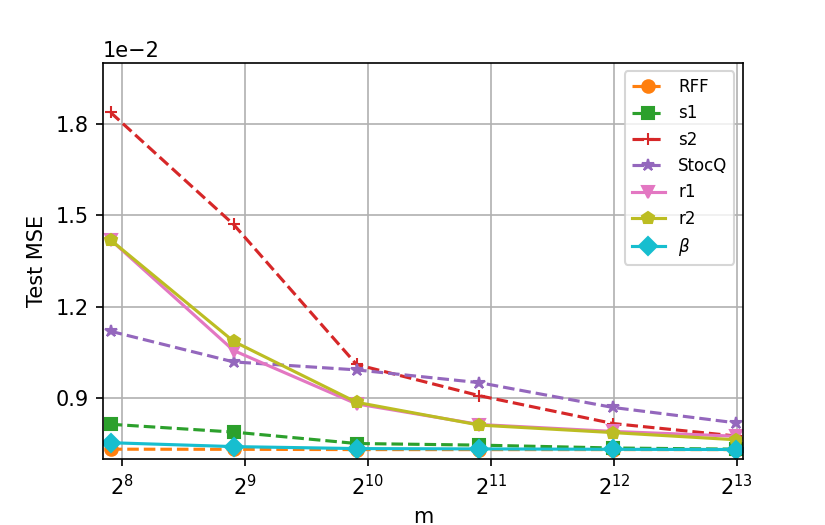
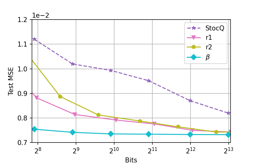
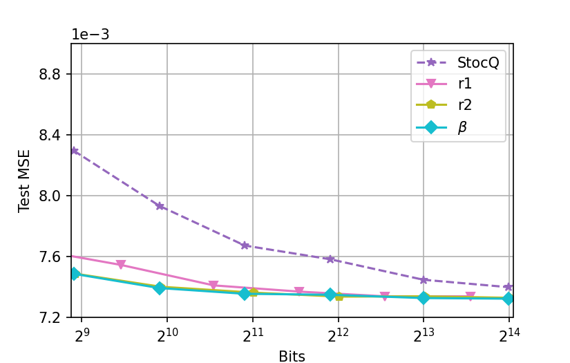
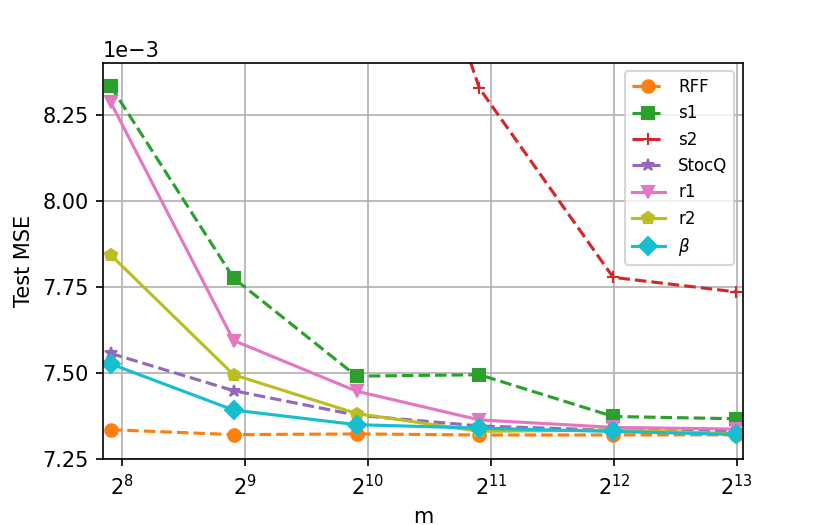
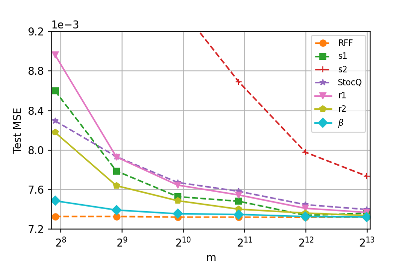
We summarize the KRR results averaging over 303030 runs for b=1𝑏1b=1 bit quantizers in Figure 1, in which solid curves represent our methods and the dashed lines depict other baselines. Note that in both cases, the noise-shaping quantizer Qβsubscript𝑄𝛽Q_{\beta} achieves the lowest test mean squared error (MSE) among all quantization schemes, and it even outperforms the semi-quantization scheme k^ssubscript^𝑘𝑠\widehat{k}_{s} with respect to the number of measurements m𝑚m. Moreover, due to the further compression advantage, QΣΔ(r)superscriptsubscript𝑄ΣΔ𝑟Q_{\Sigma\Delta}^{(r)} and Qβsubscript𝑄𝛽Q_{\beta} are more memory efficient than the fully-quantized scheme QStocQsubscript𝑄StocQQ_{\text{StocQ}} in terms of the usage of bits per sample. More experiments for b=2,3𝑏23b=2,3 can be found in Appendix C.

Refer to caption
Refer to caption
Figure 1. Kernel ridge regression with b=1𝑏1b=1. The labels RFF, s1𝑠1s1, s2𝑠2s2, StocQ, r1𝑟1r1, r2𝑟2r2, β𝛽\beta represent k^RFFsubscript^𝑘RFF\widehat{k}_{\text{RFF}}, k^ssubscript^𝑘𝑠\widehat{k}_{s} for scenarios (1), (2), k^StocQsubscript^𝑘StocQ\widehat{k}_{\text{StocQ}}, k^ΣΔ(1)superscriptsubscript^𝑘ΣΔ1\widehat{k}_{\Sigma\Delta}^{(1)}, k^ΣΔ(2)superscriptsubscript^𝑘ΣΔ2\widehat{k}_{\Sigma\Delta}^{(2)}, and k^βsubscript^𝑘𝛽\widehat{k}_{\beta} respectively.

4.2. Kernel SVM

To illustrate the performance of our methods for classification tasks, we perform Kernel SVM [32, 36] to evaluate different kernel approximations on the UCI ML hand-written digits dataset [2, 39], in which N=1797𝑁1797N=1797 grayscale images compose C=10𝐶10C=10 classes and they are vectorized to d=64𝑑64d=64 dimensional vectors. Additionally, all pixel values are scaled in the range [0,1]01[0,1] and we randomly split this dataset into 80%percent8080\% for training and 20%percent2020\% for testing. As for the classifier, we use the soft margin SVM with a regularization parameter R=1𝑅1R=1.

Note that in the binary classification case, i.e. labels yi{1,1}subscript𝑦𝑖11y_{i}\in\{-1,1\}, our goal is to learn the coefficients αisubscript𝛼𝑖\alpha_{i}, the intercept b𝑏b, and the index set of support vectors S𝑆S in a decision function during the training stage:

(19) g(x):=sign(iSαiyik(x,xi)+b).assign𝑔𝑥signsubscript𝑖Ssubscript𝛼𝑖subscript𝑦𝑖𝑘𝑥subscript𝑥𝑖𝑏g(x):=\operatorname{sign}\Bigl{(}\sum_{i\in\mathrm{S}}\alpha_{i}y_{i}k(x,x_{i})+b\Bigr{)}.

Here, we use a RBF kernel k(x,y)=exp(γxy22)𝑘𝑥𝑦𝛾superscriptsubscriptnorm𝑥𝑦22k(x,y)=\exp(-\gamma\|x-y\|_{2}^{2}) with γ=1/(dσ02)0.11𝛾1𝑑superscriptsubscript𝜎020.11\gamma=1/(d\sigma_{0}^{2})\approx 0.11 and σ02superscriptsubscript𝜎02\sigma_{0}^{2} being equal to the variance of training data. In the multi-class case, we implement the “one-versus-one” approach for multi-class classification where C(C1)2𝐶𝐶12\frac{C(C-1)}{2} classifiers are constructed and each one trains data from two classes. In our experiment, we found that a large embedding dimension p=m/λ𝑝𝑚𝜆p=m/\lambda is needed and approximations k^RFFsubscript^𝑘RFF\widehat{k}_{\text{RFF}}, k^StocQsubscript^𝑘StocQ\widehat{k}_{\text{StocQ}}, k^ΣΔ(1)superscriptsubscript^𝑘ΣΔ1\widehat{k}_{\Sigma\Delta}^{(1)} with λ=2𝜆2\lambda=2, k^ΣΔ(2)superscriptsubscript^𝑘ΣΔ2\widehat{k}_{\Sigma\Delta}^{(2)} with λ=3𝜆3\lambda=3, and k^βsubscript^𝑘𝛽\widehat{k}_{\beta} with β=1.1𝛽1.1\beta=1.1, λ=2𝜆2\lambda=2, are implemented for both training (obtaining αisubscript𝛼𝑖\alpha_{i}, b𝑏b, and S𝑆S in (19)) and testing (predicting the class of an incoming sample x𝑥x by g(x)𝑔𝑥g(x)) phases, whereas the asymmetric scheme k^ssubscript^𝑘𝑠\widehat{k}_{s} is only performed for inference with its parameters in (19) learned from k^RFFsubscript^𝑘RFF\widehat{k}_{\text{RFF}} during the training stage. Moreover, as before there are two versions of k^ssubscript^𝑘𝑠\widehat{k}_{s} used for making predictions:

  1. (1)

    Keep the support vectors as unquantized RFFs and quantize the test point x𝑥x, i.e. substitute k^s(xi,x)subscript^𝑘𝑠subscript𝑥𝑖𝑥\widehat{k}_{s}(x_{i},x) for k(x,xi)𝑘𝑥subscript𝑥𝑖k(x,x_{i}) in (19);

  2. (2)

    Quantize the support vectors and leave the testing point x𝑥x as unquantized RFFs, i.e., replace k(x,xi)𝑘𝑥subscript𝑥𝑖k(x,x_{i}) in (19) with k^s(x,xi)subscript^𝑘𝑠𝑥subscript𝑥𝑖\widehat{k}_{s}(x,x_{i}).

Refer to caption
Refer to caption
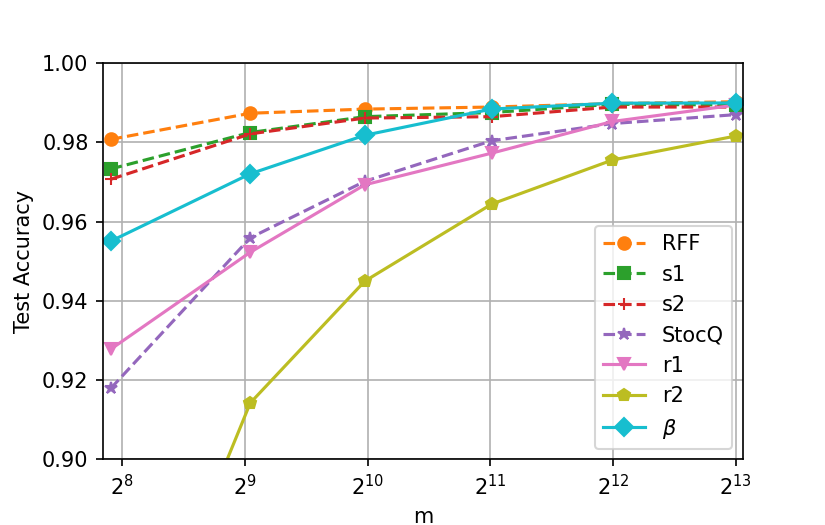
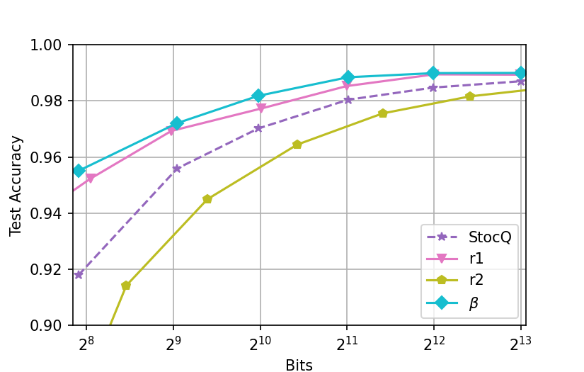
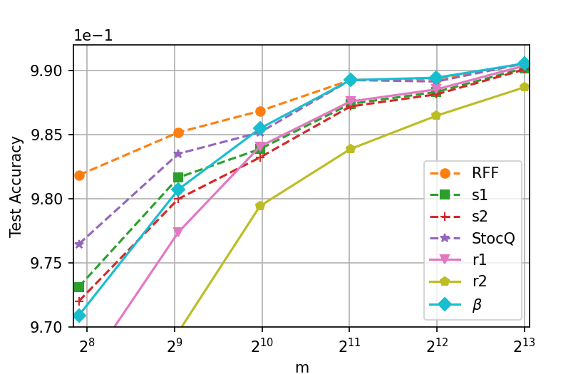
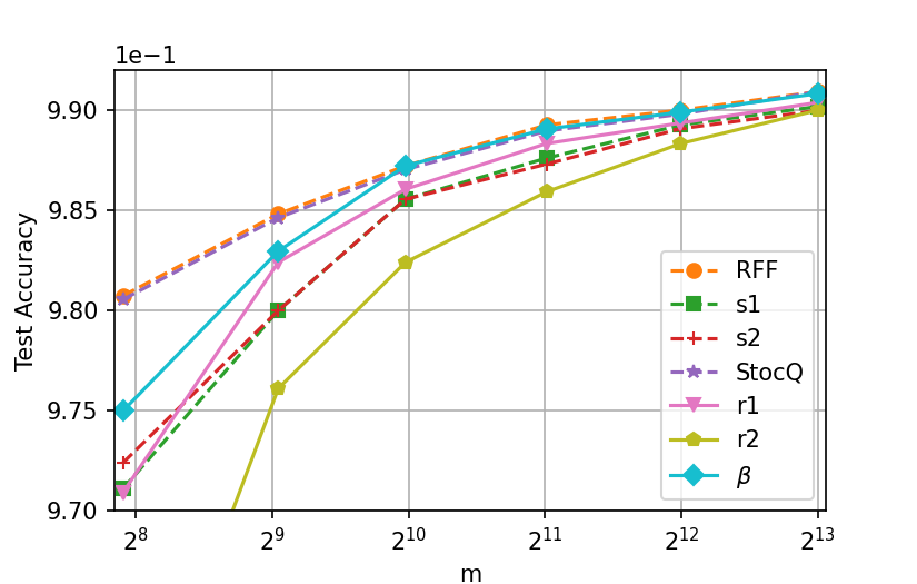
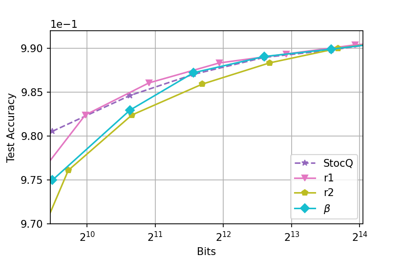
Figure 2. Kernel SVM with b=1𝑏1b=1. The labels RFF, s1𝑠1s1, s2𝑠2s2, StocQ, r1𝑟1r1, r2𝑟2r2, β𝛽\beta represent k^RFFsubscript^𝑘RFF\widehat{k}_{\text{RFF}}, k^ssubscript^𝑘𝑠\widehat{k}_{s} for scenarios (1), (2), k^StocQsubscript^𝑘StocQ\widehat{k}_{\text{StocQ}}, k^ΣΔ(1)superscriptsubscript^𝑘ΣΔ1\widehat{k}_{\Sigma\Delta}^{(1)}, k^ΣΔ(2)superscriptsubscript^𝑘ΣΔ2\widehat{k}_{\Sigma\Delta}^{(2)}, and k^βsubscript^𝑘𝛽\widehat{k}_{\beta} respectively.

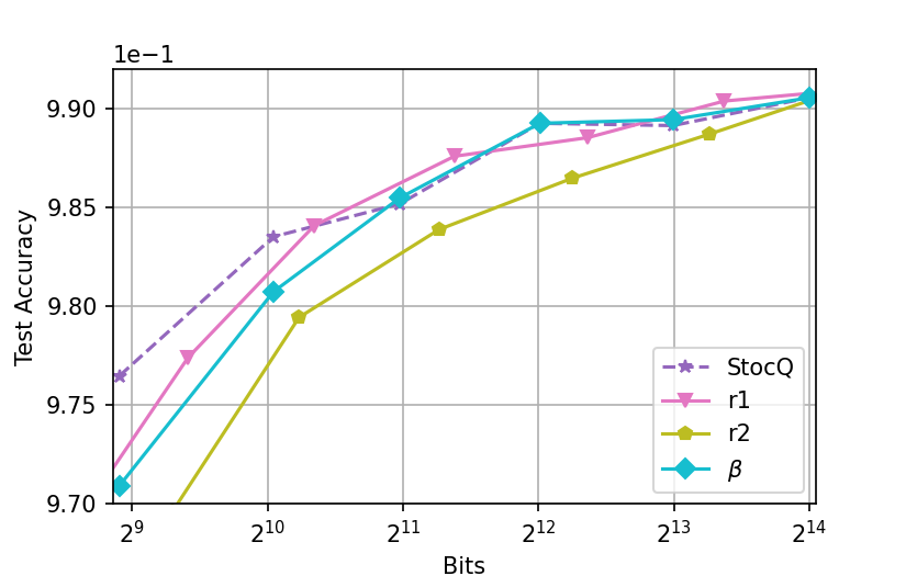
For each binary quantization scheme (with b=1𝑏1b=1), the average test accuracy over 303030 independent runs is plotted in Figure 2. We observe that, in regard to m𝑚m, Qβsubscript𝑄𝛽Q_{\beta} substantially outperforms other fully-quantized schemes including QΣΔ(r)superscriptsubscript𝑄ΣΔ𝑟Q_{\Sigma\Delta}^{(r)} and QStocQsubscript𝑄StocQQ_{\text{StocQ}}, but, as expected, it is still worse than the semi-quantized methods. Memory efficiency is characterized in the right plot by estimating the test accuracy against the storage cost (in terms of bits) per sample. Note that both Qβsubscript𝑄𝛽Q_{\beta} and QΣΔ(1)superscriptsubscript𝑄ΣΔ1Q_{\Sigma\Delta}^{(1)} have significant advantage over the baseline method QStocQsubscript𝑄StocQQ_{\text{StocQ}}, which means that our methods require less memory to achieve the same test accuracy when b=1𝑏1b=1. See Appendix C for extra experiment results with b=2,3𝑏23b=2,3.

4.3. Maximum Mean Discrepancy

Given two distributions p𝑝p and q𝑞q, and a kernel k𝑘k over 𝒳d𝒳superscript𝑑\mathcal{X}\subset\mathbb{R}^{d}, the maximum mean discrepancy (MMD) has been shown to play an important role in the two-sample test [17], by proposing the null hypothesis 0:p=q:subscript0𝑝𝑞\mathcal{H}_{0}:p=q against the alternative hypothesis 1:pq:subscript1𝑝𝑞\mathcal{H}_{1}:p\neq q. The square of MMD distance can be computed by

MMDk2(p,q)=𝔼x,x(k(x,x))+𝔼y,y(k(y,y))2𝔼x,y(k(x,y))superscriptsubscriptMMD𝑘2𝑝𝑞subscript𝔼𝑥superscript𝑥𝑘𝑥superscript𝑥subscript𝔼𝑦superscript𝑦𝑘𝑦superscript𝑦2subscript𝔼𝑥𝑦𝑘𝑥𝑦\mathrm{MMD}_{k}^{2}(p,q)=\mathbb{E}_{x,x^{\prime}}(k(x,x^{\prime}))+\mathbb{E}_{y,y^{\prime}}(k(y,y^{\prime}))-2\mathbb{E}_{x,y}(k(x,y))

where x,xiidp𝑥superscript𝑥𝑖𝑖𝑑similar-to𝑝x,x^{\prime}\overset{iid}{\sim}p and y,yiidq𝑦superscript𝑦𝑖𝑖𝑑similar-to𝑞y,y^{\prime}\overset{iid}{\sim}q. Here, we set k𝑘k to a RBF kernel, which is characteristic [35] implying that MMDk(p,q)subscriptMMD𝑘𝑝𝑞\mathrm{MMD}_{k}(p,q) is metric, i.e. MMDk(p,q)=0p=qiffsubscriptMMD𝑘𝑝𝑞0𝑝𝑞\mathrm{MMD}_{k}(p,q)=0\iff p=q, and the following hypothesis test is consistent.
Refer to caption
(a) True distributions: p𝑝p and q𝑞q
Refer to caption
(b) Samples of size 606060 from p𝑝p, q𝑞q
Refer to caption
(c) Counts vs MMD values
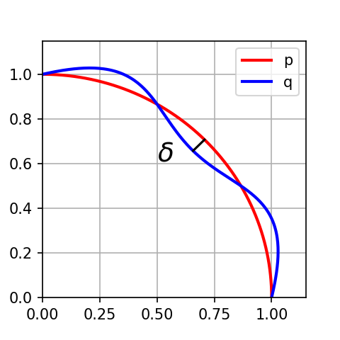
Figure 3. Two distributions and the MMD values based on the RBF kernel.
Refer to caption
Refer to caption
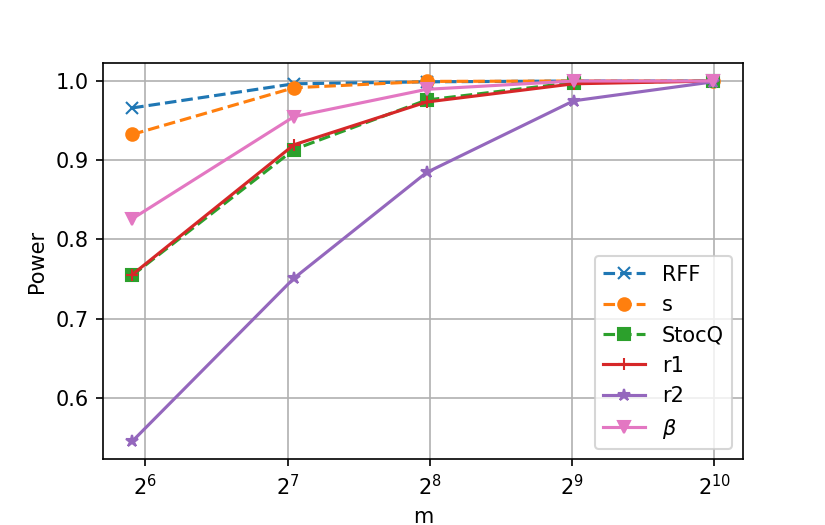
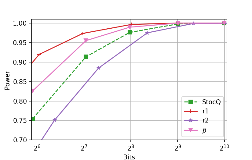
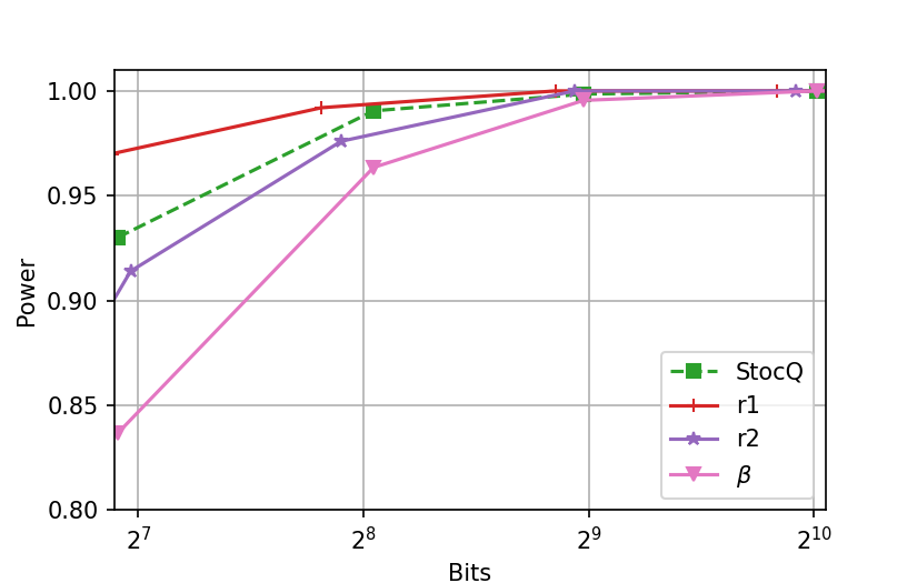
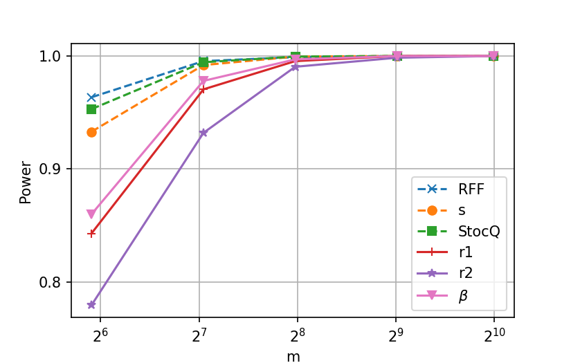
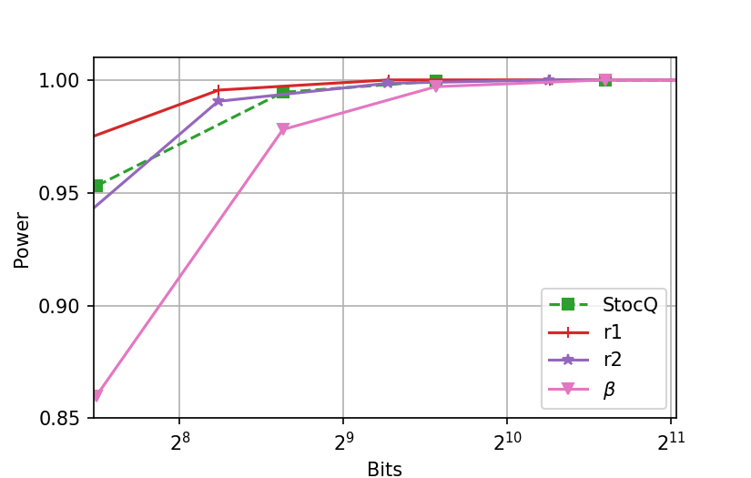
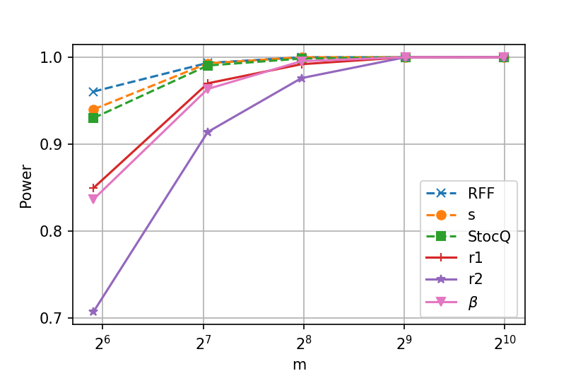
Figure 4. Power of the permutation test with b=1𝑏1b=1. The labels RFF, s𝑠s, StocQ, r1𝑟1r1, r2𝑟2r2, β𝛽\beta represent k^RFFsubscript^𝑘RFF\widehat{k}_{\text{RFF}}, k^ssubscript^𝑘𝑠\widehat{k}_{s}, k^StocQsubscript^𝑘StocQ\widehat{k}_{\text{StocQ}}, k^ΣΔ(1)superscriptsubscript^𝑘ΣΔ1\widehat{k}_{\Sigma\Delta}^{(1)}, k^ΣΔ(2)superscriptsubscript^𝑘ΣΔ2\widehat{k}_{\Sigma\Delta}^{(2)}, and k^βsubscript^𝑘𝛽\widehat{k}_{\beta} respectively.

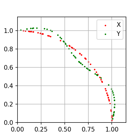
In our experiment, the distribution p𝑝p is supported on a quadrant of the unit circle while q𝑞q is generated by perturbing p𝑝p by a gap of size δ𝛿\delta at various regions, see Figure 3(a). Let n=60𝑛60n=60 and choose finite samples X={x1,,xn}p𝑋subscript𝑥1subscript𝑥𝑛similar-to𝑝X=\{x_{1},\ldots,x_{n}\}\sim p and Y={y1,,yn}q𝑌subscript𝑦1subscript𝑦𝑛similar-to𝑞Y=\{y_{1},\ldots,y_{n}\}\sim q. Then MMDk(p,q)subscriptMMD𝑘𝑝𝑞\mathrm{MMD}_{k}(p,q) can be estimated by

(20) MMD^k2(X,Y):=1n2i,j=1nk(xi,xj)+1n2i,j=1nk(yi,yj)2n2i,j=1nk(xi,yj).assignsuperscriptsubscript^MMD𝑘2𝑋𝑌1superscript𝑛2superscriptsubscript𝑖𝑗1𝑛𝑘subscript𝑥𝑖subscript𝑥𝑗1superscript𝑛2superscriptsubscript𝑖𝑗1𝑛𝑘subscript𝑦𝑖subscript𝑦𝑗2superscript𝑛2superscriptsubscript𝑖𝑗1𝑛𝑘subscript𝑥𝑖subscript𝑦𝑗\widehat{\mathrm{MMD}}_{k}^{2}(X,Y):=\frac{1}{n^{2}}\sum_{i,j=1}^{n}k(x_{i},x_{j})+\frac{1}{n^{2}}\sum_{i,j=1}^{n}k(y_{i},y_{j})-\frac{2}{n^{2}}\sum_{i,j=1}^{n}k(x_{i},y_{j}).

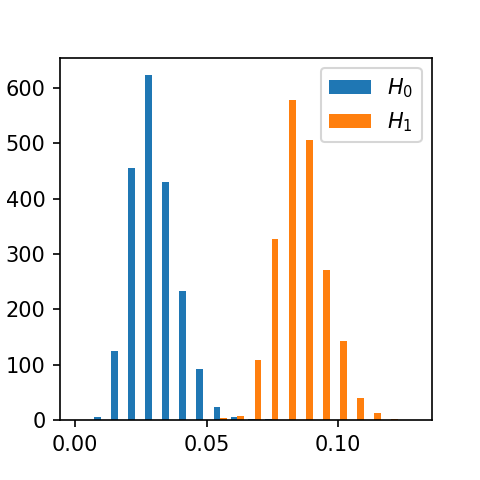
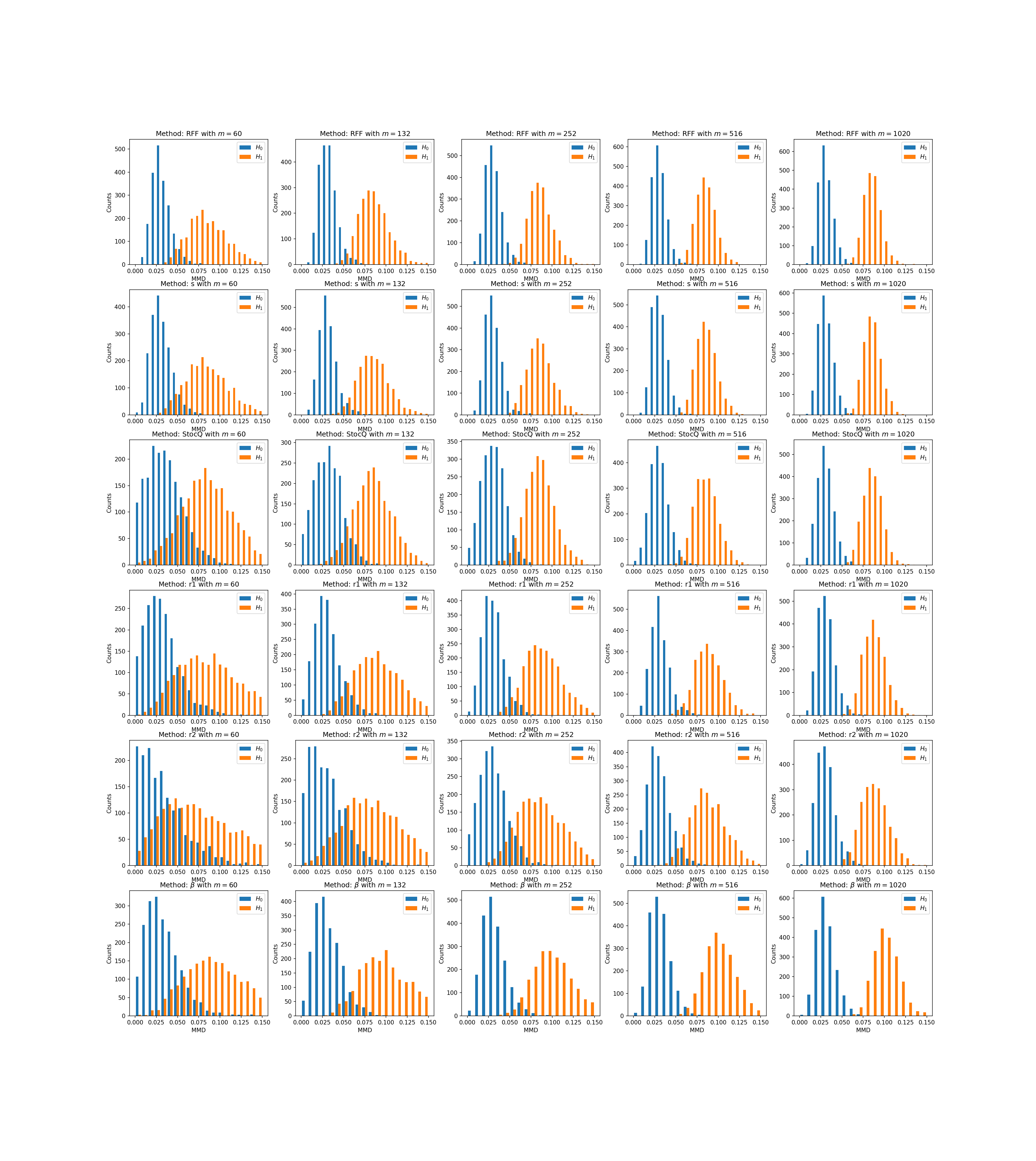
Under the null hypothesis 0subscript0\mathcal{H}_{0}, one can get the empirical distribution of (20) by reshuffling the data samples XY𝑋𝑌X\cup Y many times (t=2000𝑡2000t=2000) and recomputing MMD^k2(X,Y)superscriptsubscript^MMD𝑘2superscript𝑋superscript𝑌\widehat{\mathrm{MMD}}_{k}^{2}(X^{\prime},Y^{\prime}) on each partition XYsuperscript𝑋superscript𝑌X^{\prime}\cup Y^{\prime}. For a significance level of α=0.05𝛼0.05\alpha=0.05, 0subscript0\mathcal{H}_{0} is rejected if the original MMD^k2(X,Y)superscriptsubscript^MMD𝑘2𝑋𝑌\widehat{\mathrm{MMD}}_{k}^{2}(X,Y) is greater than the (1α)1𝛼(1-\alpha) quantile from the empirical distribution. Figure 3(c) shows that the empirical distributions of (20) under both 0subscript0\mathcal{H}_{0} and 1subscript1\mathcal{H}_{1} are separated well, where we use the ground truth RBF kernel with small bandwidth σ=0.05𝜎0.05\sigma=0.05.

In order to compare different quantization methods when b=1𝑏1b=1, we use the following approximations with optimal λ𝜆\lambda to perform the permutation test: k^RFFsubscript^𝑘RFF\widehat{k}_{\text{RFF}}, k^StocQsubscript^𝑘StocQ\widehat{k}_{\text{StocQ}}, k^ΣΔ(1)superscriptsubscript^𝑘ΣΔ1\widehat{k}_{\Sigma\Delta}^{(1)} with λ=4𝜆4\lambda=4, k^ΣΔ(2)superscriptsubscript^𝑘ΣΔ2\widehat{k}_{\Sigma\Delta}^{(2)} with λ=5𝜆5\lambda=5, and k^βsubscript^𝑘𝛽\widehat{k}_{\beta} with β=1.5𝛽1.5\beta=1.5, λ=4𝜆4\lambda=4. Due to the symmetry in (20), k^ssubscript^𝑘𝑠\widehat{k}_{s} can be implemented without worrying about the order of inputs. Additionally, if the probability of Type II error, i.e. false negative rate, is denoted by β𝛽\beta, then the statistical power of our test is defined by

power=1β=P(reject0|1istrue)power1𝛽Pconditionalrejectsubscript0subscript1istrue\mathrm{power}=1-\beta=\mathrm{P}(\mathrm{reject}\,\mathcal{H}_{0}|\,\mathcal{H}_{1}\mathrm{is\,true})

In other words, the power equals to the portion of MMD values under 1subscript1\mathcal{H}_{1} that are greater than the (1α)1𝛼(1-\alpha) quantile of MMD distribution under 0subscript0\mathcal{H}_{0}. In Figure 4, we observe that, compared with other fully-quantized schemes, Qβsubscript𝑄𝛽Q_{\beta} has the greatest power in terms of m𝑚m. The performance of semi-quantized scheme is pretty close to the plain RFF approximation while it requires more storage space, as discussed in Section 3. Moreover, Figure 5 presents the corresponding changes of the MMD distributions under 0subscript0\mathcal{H}_{0} and 1subscript1\mathcal{H}_{1}, in which the overlap between the two distributions is considerably reduced as m𝑚m increases. Regarding the number of bits per sample, both QΣΔ(1)superscriptsubscript𝑄ΣΔ1Q_{\Sigma\Delta}^{(1)} and Qβsubscript𝑄𝛽Q_{\beta} have remarkable advantage over QStocQsubscript𝑄StocQQ_{\text{StocQ}}. Extra results related to b=2,3𝑏23b=2,3 can be found in Appendix C.

Refer to caption
Figure 5. The empirical distributions of MMD values under 0subscript0\mathcal{H}_{0} and 1subscript1\mathcal{H}_{1}.

5. Conclusion

In order to reduce memory requirement for training and storing kernel machines, we proposed a framework of using Sigma-Delta and distributed noise-shaping quantization schemes, QΣΔ(r)superscriptsubscript𝑄ΣΔ𝑟Q_{\Sigma\Delta}^{(r)} and Qβsubscript𝑄𝛽Q_{\beta}, to approximate shift-invariant kernels. We have shown that these fully deterministic quantization schemes are capable of saving more bits than other baselines without compromising the performance. Importantly, we showed that, for all pairs of signals from an infinite low-complexity set, the approximations have uniform probabilistic error bounds yielding an exponential decay as the number of bits used increases. Empirically, we illustrated across popular kernel machines that the proposed quantization methods achieve strong performance both as a function of the dimension of the RFF embedding, and the number of bits used, especially in the case of binary embedding.

Data Availability Statement

The data underlying this article are available in the UCI Machine Learning Repository, at https://archive.ics.uci.edu/ml/datasets/Optical+Recognition+of+Handwritten+Digits

Funding

JZ was partially supported by grants NSF DMS 2012546 and 2012266. AC was partially supported by NSF DMS 1819222, 2012266. RS was partially supported by NSF DMS 2012546 and a UCSD senate research award.

References

  • Agrawal et al. [2019] R. Agrawal, T. Campbell, J. Huggins, and T. Broderick. Data-dependent compression of random features for large-scale kernel approximation. In The 22nd International Conference on Artificial Intelligence and Statistics, pages 1822–1831. PMLR, 2019.
  • Alpaydin and Kaynak [1998] E. Alpaydin and C. Kaynak. Cascading classifiers. Kybernetika, 34(4):369–374, 1998.
  • Avron et al. [2017a] H. Avron, K. L. Clarkson, and D. P. Woodruff. Faster kernel ridge regression using sketching and preconditioning. SIAM Journal on Matrix Analysis and Applications, 38(4):1116–1138, 2017a.
  • Avron et al. [2017b] H. Avron, M. Kapralov, C. Musco, C. Musco, A. Velingker, and A. Zandieh. Random fourier features for kernel ridge regression: Approximation bounds and statistical guarantees. In International Conference on Machine Learning, pages 253–262. PMLR, 2017b.
  • Bach [2017] F. Bach. On the equivalence between kernel quadrature rules and random feature expansions. The Journal of Machine Learning Research, 18(1):714–751, 2017.
  • Benedetto et al. [2006a] J. J. Benedetto, A. M. Powell, and Ö. Yılmaz. Second-order sigma–delta (σ𝜎\sigmaδ𝛿\delta) quantization of finite frame expansions. Applied and Computational Harmonic Analysis, 20(1):126–148, 2006a.
  • Benedetto et al. [2006b] J. J. Benedetto, A. M. Powell, and O. Yilmaz. Sigma-delta quantization and finite frames. IEEE Transactions on Information Theory, 52(5):1990–2005, 2006b.
  • Boufounos and Rane [2013] P. T. Boufounos and S. Rane. Efficient coding of signal distances using universal quantized embeddings. In DCC, pages 251–260, 2013.
  • Chou and Güntürk [2016] E. Chou and C. S. Güntürk. Distributed noise-shaping quantization: I. beta duals of finite frames and near-optimal quantization of random measurements. Constructive Approximation, 44(1):1–22, 2016.
  • Chou and Güntürk [2017] E. Chou and C. S. Güntürk. Distributed noise-shaping quantization: Ii. classical frames. In Excursions in Harmonic Analysis, Volume 5, pages 179–198. Springer, 2017.
  • Chou et al. [2015] E. Chou, C. S. Güntürk, F. Krahmer, R. Saab, and Ö. Yılmaz. Noise-shaping quantization methods for frame-based and compressive sampling systems. Sampling theory, a renaissance, pages 157–184, 2015.
  • Cucker and Smale [2002] F. Cucker and S. Smale. On the mathematical foundations of learning. Bulletin of the American mathematical society, 39(1):1–49, 2002.
  • Danzer [1963] L. Danzer. ” helly’s theorem and its relatives,” in convexity. In Proc. Symp. Pure Math., volume 7, pages 101–180. Amer. Math. Soc., 1963.
  • Daubechies and DeVore [2003] I. Daubechies and R. DeVore. Approximating a bandlimited function using very coarsely quantized data: A family of stable sigma-delta modulators of arbitrary order. Annals of mathematics, pages 679–710, 2003.
  • Deift et al. [2011] P. Deift, F. Krahmer, and C. S. Güntürk. An optimal family of exponentially accurate one-bit sigma-delta quantization schemes. Communications on Pure and Applied Mathematics, 64(7):883–919, 2011.
  • Foucart and Rauhut [2013] S. Foucart and H. Rauhut. A Mathematical Introduction to Compressive Sensing. Springer, 2013.
  • Gretton et al. [2012] A. Gretton, K. M. Borgwardt, M. J. Rasch, B. Schölkopf, and A. Smola. A kernel two-sample test. The Journal of Machine Learning Research, 13(1):723–773, 2012.
  • Güntürk [2003] C. S. Güntürk. One-bit sigma-delta quantization with exponential accuracy. Communications on Pure and Applied Mathematics: A Journal Issued by the Courant Institute of Mathematical Sciences, 56(11):1608–1630, 2003.
  • Güntürk et al. [2013] C. S. Güntürk, M. Lammers, A. M. Powell, R. Saab, and Ö. Yılmaz. Sobolev duals for random frames and σ𝜎\sigmaδ𝛿\delta quantization of compressed sensing measurements. Foundations of Computational mathematics, 13(1):1–36, 2013.
  • Huynh [2016] T. Huynh. Accurate quantization in redundant systems: From frames to compressive sampling and phase retrieval. PhD thesis, New York University, 2016.
  • Huynh and Saab [2020] T. Huynh and R. Saab. Fast binary embeddings and quantized compressed sensing with structured matrices. Communications on Pure and Applied Mathematics, 73(1):110–149, 2020.
  • Krahmer et al. [2012] F. Krahmer, R. Saab, and R. Ward. Root-exponential accuracy for coarse quantization of finite frame expansions. IEEE transactions on information theory, 58(2):1069–1079, 2012.
  • Li and Li [2021] X. Li and P. Li. Quantization algorithms for random fourier features. arXiv preprint arXiv:2102.13079, 2021.
  • Lin [2007] C.-J. Lin. Large-scale kernel machines. MIT press, 2007.
  • Liu et al. [2020] F. Liu, X. Huang, Y. Chen, and J. A. Suykens. Random features for kernel approximation: A survey in algorithms, theory, and beyond. arXiv preprint arXiv:2004.11154, 2020.
  • Loomis [2013] L. H. Loomis. Introduction to abstract harmonic analysis. Courier Corporation, 2013.
  • May et al. [2019] A. May, A. B. Garakani, Z. Lu, D. Guo, K. Liu, A. Bellet, L. Fan, M. Collins, D. Hsu, B. Kingsbury, M. Picheny, and F. Sha. Kernel approximation methods for speech recognition. Journal of Machine Learning Research, 20(59):1–36, 2019. URL http://jmlr.org/papers/v20/17-026.html.
  • Murphy [2012] K. P. Murphy. Machine learning: a probabilistic perspective. MIT press, 2012.
  • Rahimi and Recht [2007] A. Rahimi and B. Recht. Random features for large-scale kernel machines. Advances in neural information processing systems, 20:1177–1184, 2007.
  • Rudi and Rosasco [2017] A. Rudi and L. Rosasco. Generalization properties of learning with random features. In NIPS, pages 3215–3225, 2017.
  • Schellekens and Jacques [2020] V. Schellekens and L. Jacques. Breaking the waves: asymmetric random periodic features for low-bitrate kernel machines. arXiv preprint arXiv:2004.06560, 2020.
  • Scholkopf and Smola [2018] B. Scholkopf and A. J. Smola. Learning with kernels: support vector machines, regularization, optimization, and beyond. Adaptive Computation and Machine Learning series, 2018.
  • Shawe-Taylor et al. [2004] J. Shawe-Taylor, N. Cristianini, et al. Kernel methods for pattern analysis. Cambridge university press, 2004.
  • Sriperumbudur and Szabó [2015] B. K. Sriperumbudur and Z. Szabó. Optimal rates for random fourier features. In Proceedings of the 28th International Conference on Neural Information Processing Systems-Volume 1, pages 1144–1152, 2015.
  • Sriperumbudur et al. [2010] B. K. Sriperumbudur, A. Gretton, K. Fukumizu, B. Schölkopf, and G. R. Lanckriet. Hilbert space embeddings and metrics on probability measures. The Journal of Machine Learning Research, 11:1517–1561, 2010.
  • Steinwart and Christmann [2008] I. Steinwart and A. Christmann. Support vector machines. Springer Science & Business Media, 2008.
  • Sutherland and Schneider [2015] D. J. Sutherland and J. Schneider. On the error of random fourier features. In Proceedings of the Thirty-First Conference on Uncertainty in Artificial Intelligence, pages 862–871, 2015.
  • Tu et al. [2016] S. Tu, R. Roelofs, S. Venkataraman, and B. Recht. Large scale kernel learning using block coordinate descent. arXiv preprint arXiv:1602.05310, 2016.
  • Xu et al. [1992] L. Xu, A. Krzyzak, and C. Y. Suen. Methods of combining multiple classifiers and their applications to handwriting recognition. IEEE transactions on systems, man, and cybernetics, 22(3):418–435, 1992.
  • Zhang and Saab [2021] J. Zhang and R. Saab. Faster binary embeddings for preserving euclidean distances. In International Conference on Learning Representations, 2021. URL https://openreview.net/forum?id=YCXrx6rRCXO.
  • Zhang et al. [2019] J. Zhang, A. May, T. Dao, and C. Ré. Low-precision random fourier features for memory-constrained kernel approximation. In The 22nd International Conference on Artificial Intelligence and Statistics, pages 1264–1274. PMLR, 2019.

Appendix A Stable Quantization Methods

The general definition for stable QΣΔ(r)superscriptsubscript𝑄ΣΔ𝑟Q_{\Sigma\Delta}^{(r)}. Although it is a non-trivial task to design a stable QΣΔ(r)superscriptsubscript𝑄ΣΔ𝑟Q_{\Sigma\Delta}^{(r)} for r>1𝑟1r>1, families of ΣΔΣΔ\Sigma\Delta quantization schemes that achieve this goal have been designed [14, 15, 18], and we adopt the version in [15]. Specifically, an r𝑟r-th order ΣΔΣΔ\Sigma\Delta quantization scheme may also arise from the following difference equation

(21) yq=Hv𝑦𝑞𝐻𝑣y-q=H*v

where * is the convolution operator and the sequence H:=Drgassign𝐻superscript𝐷𝑟𝑔H:=D^{r}g with g1𝑔superscript1g\in\ell^{1}. Then any bounded solution v𝑣v of (21) gives rise to a bounded solution u𝑢u of (11) via u=gv𝑢𝑔𝑣u=g*v. By change of variables, (11) can be reformulated as (21). By choosing a proper filter h:=δ(0)Hassignsuperscript𝛿0𝐻h:=\delta^{(0)}-H, where δ(0)superscript𝛿0\delta^{(0)} denotes the Kronecker delta sequence supported at 00, one can implement (21) by vi=(hv)i+yiqisubscript𝑣𝑖subscript𝑣𝑖subscript𝑦𝑖subscript𝑞𝑖v_{i}=(h*v)_{i}+y_{i}-q_{i} and the corresponding stable quantization scheme QΣΔ(r)superscriptsubscript𝑄ΣΔ𝑟Q_{\Sigma\Delta}^{(r)} reads as

(22) {qi=Q((hv)i+yi),vi=(hv)i+yiqi.casessubscript𝑞𝑖𝑄subscript𝑣𝑖subscript𝑦𝑖otherwisesubscript𝑣𝑖subscript𝑣𝑖subscript𝑦𝑖subscript𝑞𝑖otherwise\begin{cases}q_{i}=Q((h*v)_{i}+y_{i}),\\ v_{i}=(h*v)_{i}+y_{i}-q_{i}.\end{cases}

Furthermore, the above design leads to the following result from [15, 22], which exploits the constant c(K,μ,r)𝑐𝐾𝜇𝑟c(K,\mu,r) to bound usubscriptnorm𝑢\|u\|_{\infty}.

Proposition A.1.

There exists a universal constant C>0𝐶0C>0 such that the ΣΔΣΔ\Sigma\Delta schemes (10) and (22) with alphabet 𝒜𝒜\mathcal{A} in (4), are stable, and

yμ<1uc(K,r):=CC1rrr2K1,subscriptnorm𝑦𝜇1subscriptnorm𝑢𝑐𝐾𝑟assign𝐶superscriptsubscript𝐶1𝑟superscript𝑟𝑟2𝐾1\|y\|_{\infty}\leq\mu<1\Longrightarrow\|u\|_{\infty}\leq c(K,r):=\frac{CC_{1}^{r}r^{r}}{2K-1},

where C1=(π2(cosh1γ)2eπ)subscript𝐶1superscript𝜋2superscriptsuperscript1𝛾2𝑒𝜋C_{1}=\bigl{(}\bigl{\lceil}\frac{\pi^{2}}{(\cosh^{-1}\gamma)^{2}}\bigr{\rceil}\frac{e}{\pi}\bigr{)} with γ:=2K(2K1)μassign𝛾2𝐾2𝐾1𝜇\gamma:=2K-(2K-1)\mu.

Note that even with the b=1𝑏1b=1 bit alphabet, i.e. K=1𝐾1K=1 and 𝒜={1,1}𝒜11\mathcal{A}=\{-1,1\}, stability can be guaranteed with

yμ<1uCC1rrr.formulae-sequencesubscriptnorm𝑦𝜇1subscriptnorm𝑢𝐶superscriptsubscript𝐶1𝑟superscript𝑟𝑟\|y\|_{\infty}\leq\mu<1\quad\Longrightarrow\quad\|u\|_{\infty}\leq C\cdot C_{1}^{r}\cdot r^{r}.

The stability of Qβsubscript𝑄𝛽Q_{\beta}. The relevant result for stability of the noise-shaping quantization schemes (13) is the following proposition, which can be simply proved by induction or can be found in [10].

Proposition A.2.

The noise-shaping scheme (13) with alphabet 𝒜𝒜\mathcal{A} in (4) is stable and

y2Kβ2K1uc(K,β):=12K1.subscriptnorm𝑦2𝐾𝛽2𝐾1subscriptnorm𝑢𝑐𝐾𝛽assign12𝐾1\|y\|_{\infty}\leq\frac{2K-\beta}{2K-1}\Longrightarrow\|u\|_{\infty}\leq c(K,\beta):=\frac{1}{2K-1}.

Appendix B A comparison of kernel approximations

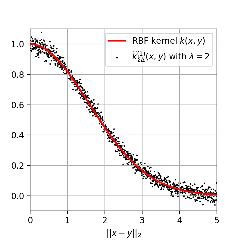
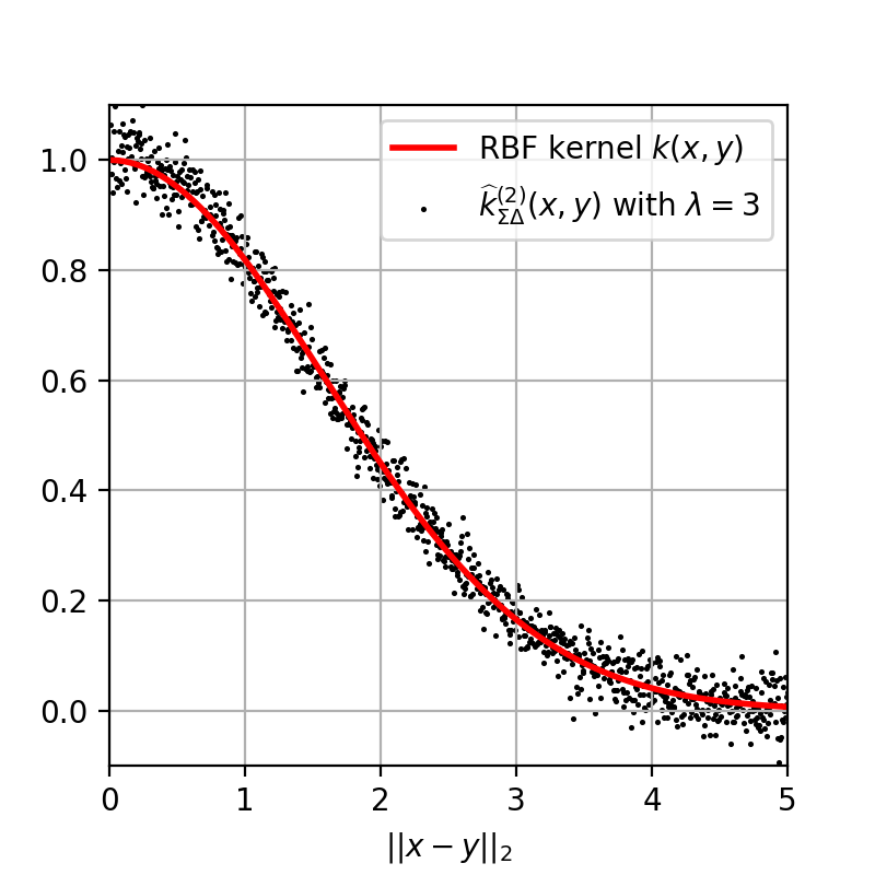
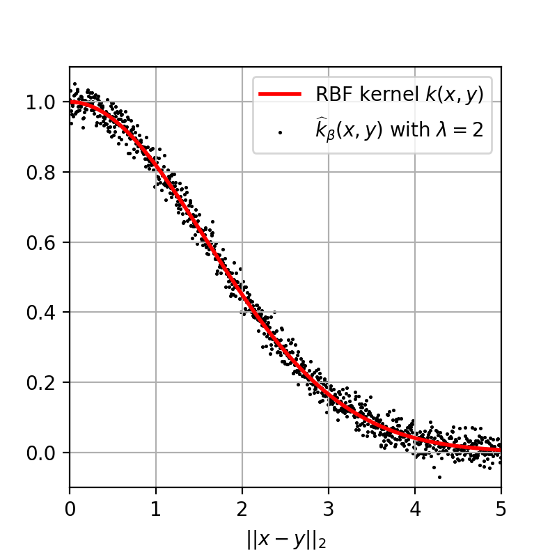
In Figure 6, we evaluate approximated kernels (8) and (9) in Section 1 on n=1000𝑛1000n=1000 pairs of points {xi,yi}i=1nsuperscriptsubscriptsubscript𝑥𝑖subscript𝑦𝑖𝑖1𝑛\{x_{i},y_{i}\}_{i=1}^{n} in dsuperscript𝑑\mathbb{R}^{d} with d=50𝑑50d=50 such that for each i𝑖i

xi𝒩(0,Id),ui𝒩(0,Id),yi=xi+5inuiui2.formulae-sequencesimilar-tosubscript𝑥𝑖𝒩0subscript𝐼𝑑formulae-sequencesimilar-tosubscript𝑢𝑖𝒩0subscript𝐼𝑑subscript𝑦𝑖subscript𝑥𝑖5𝑖𝑛subscript𝑢𝑖subscriptnormsubscript𝑢𝑖2x_{i}\sim\mathcal{N}(0,I_{d}),\quad u_{i}\sim\mathcal{N}(0,I_{d}),\quad y_{i}=x_{i}+\frac{5i}{n}\cdot\frac{u_{i}}{\|u_{i}\|_{2}}.

Moreover, each data point xisubscript𝑥𝑖x_{i} is represented by m=3000𝑚3000m=3000 RFF features and we use 333-bit quantizers to guarantee good performance for all methods. The target RBF kernel (red curves) is k(x,y)=exp(xy22/2σ2)𝑘𝑥𝑦superscriptsubscriptnorm𝑥𝑦222superscript𝜎2k(x,y)=\exp(-\|x-y\|_{2}^{2}/2\sigma^{2}) with γ:=1/2σ2=15assign𝛾12superscript𝜎215\gamma:=1/2\sigma^{2}=\frac{1}{5} and note that the approximations (black dots) have their 2subscript2\ell_{2} distances xy2subscriptnorm𝑥𝑦2\|x-y\|_{2} uniformly distributed in the range [0,5]05[0,5]. We see that both k^ΣΔ(r)superscriptsubscript^𝑘ΣΔ𝑟\widehat{k}_{\Sigma\Delta}^{(r)} and k^βsubscript^𝑘𝛽\widehat{k}_{\beta} can approximate k𝑘k well.

Refer to caption
(a) k^ΣΔ(r)(x,y)subscriptsuperscript^𝑘𝑟ΣΔ𝑥𝑦\widehat{k}^{(r)}_{\Sigma\Delta}(x,y) with r=1𝑟1r=1
Refer to caption
(b) k^ΣΔ(r)(x,y)subscriptsuperscript^𝑘𝑟ΣΔ𝑥𝑦\widehat{k}^{(r)}_{\Sigma\Delta}(x,y) with r=2𝑟2r=2
Refer to caption
(c) k^β(x,y)subscript^𝑘𝛽𝑥𝑦\widehat{k}_{\beta}(x,y) with β=1.1𝛽1.1\beta=1.1

.

Figure 6. Kernel Approximations with b=3𝑏3b=3.

Appendix C More Figures in Section 4

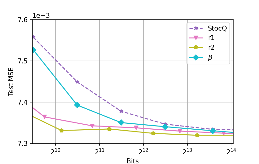
KRR. In Figure 7 and Figure 8, we show the KRR results for b=2𝑏2b=2 and b=3𝑏3b=3 respectively. Same as in the Section 4, we see that the proposed methods QΣΔ(r)superscriptsubscript𝑄ΣΔ𝑟Q_{\Sigma\Delta}^{(r)} and Qβsubscript𝑄𝛽Q_{\beta} have strong performance in terms of m𝑚m and the number of bits used for each sample.
Refer to caption
Refer to caption
Figure 7. Kernel ridge regression with b=2𝑏2b=2.
Refer to caption
Refer to caption
Figure 8. Kernel ridge regression with b=3𝑏3b=3.

Kernel SVM. Figure 9 and Figure 10 illustrate the performance of kernel SVM with b=2𝑏2b=2 and b=3𝑏3b=3 respectively. As we expect, the gap across various schemes shrinks when we use multibit quantizers, where QStocQsubscript𝑄StocQQ_{\text{StocQ}} is comparable with QΣΔ(r)superscriptsubscript𝑄ΣΔ𝑟Q_{\Sigma\Delta}^{(r)} and Qβsubscript𝑄𝛽Q_{\beta}.

Refer to caption
Refer to caption
Figure 9. Kernel SVM with b=2𝑏2b=2.
Refer to caption
Refer to caption
Figure 10. Kernel SVM with b=3𝑏3b=3.

MMD. As a continuation of the two-sample test in Section 4, Figure 11 and Figure 12 imply that both semi-quantized scheme and QStocQsubscript𝑄StocQQ_{\text{StocQ}} have better performance with respect to m𝑚m, while QΣΔ(r)superscriptsubscript𝑄ΣΔ𝑟Q_{\Sigma\Delta}^{(r)} can save more memory than other quantization methods.
Refer to caption
Refer to caption
Figure 11. Power of the permutation test with b=2𝑏2b=2.
Refer to caption
Refer to caption
Figure 12. Power of the permutation test with b=3𝑏3b=3.

Appendix D Proof of Theorem 3.1

Given x,y𝒳d𝑥𝑦𝒳superscript𝑑x,y\in\mathcal{X}\subset\mathbb{R}^{d}, we use either stable QΣΔ(r)superscriptsubscript𝑄ΣΔ𝑟Q_{\Sigma\Delta}^{(r)} or stable Qβsubscript𝑄𝛽Q_{\beta} to quantize their RFFs z(x)𝑧𝑥z(x), z(y)𝑧𝑦z(y) as in (2). Then we get quantized sequences

qΣΔ(r)(x):=QΣΔ(r)(z(x)),qΣΔ(r)(y):=QΣΔ(r)(z(y)),orqβ(x):=Qβ(z(x)),qβ(y):=Qβ(z(y)),formulae-sequenceassignsuperscriptsubscript𝑞ΣΔ𝑟𝑥superscriptsubscript𝑄ΣΔ𝑟𝑧𝑥formulae-sequenceassignsuperscriptsubscript𝑞ΣΔ𝑟𝑦superscriptsubscript𝑄ΣΔ𝑟𝑧𝑦orformulae-sequenceassignsubscript𝑞𝛽𝑥subscript𝑄𝛽𝑧𝑥assignsubscript𝑞𝛽𝑦subscript𝑄𝛽𝑧𝑦q_{\Sigma\Delta}^{(r)}(x):=Q_{\Sigma\Delta}^{(r)}(z(x)),\quad q_{\Sigma\Delta}^{(r)}(y):=Q_{\Sigma\Delta}^{(r)}(z(y)),\quad\text{or}\quad q_{\beta}(x):=Q_{\beta}(z(x)),\quad q_{\beta}(y):=Q_{\beta}(z(y)),

and expect that both

k^ΣΔ(r)(x,y)=V~ΣΔqΣΔ(r)(x),V~ΣΔqΣΔ(r)(y),k^β(x,y)=V~βqβ(x),V~βqβ(y)formulae-sequencesubscriptsuperscript^𝑘𝑟ΣΔ𝑥𝑦subscript~𝑉ΣΔsuperscriptsubscript𝑞ΣΔ𝑟𝑥subscript~𝑉ΣΔsuperscriptsubscript𝑞ΣΔ𝑟𝑦subscript^𝑘𝛽𝑥𝑦subscript~𝑉𝛽subscript𝑞𝛽𝑥subscript~𝑉𝛽subscript𝑞𝛽𝑦\widehat{k}^{(r)}_{\Sigma\Delta}(x,y)=\langle\widetilde{V}_{\Sigma\Delta}q_{\Sigma\Delta}^{(r)}(x),\widetilde{V}_{\Sigma\Delta}q_{\Sigma\Delta}^{(r)}(y)\rangle,\quad\widehat{k}_{\beta}(x,y)=\langle\widetilde{V}_{\beta}q_{\beta}(x),\widetilde{V}_{\beta}q_{\beta}(y)\rangle

approximate the ground truth k(x,y)𝑘𝑥𝑦k(x,y) well.

In the case of ΣΔΣΔ\Sigma\Delta quantization, by (11), one can get

V~ΣΔqΣΔ(r)(x)=V~ΣΔz(x)V~ΣΔDrux,V~ΣΔqΣΔ(r)(y)=V~ΣΔz(y)V~ΣΔDruy.formulae-sequencesubscript~𝑉ΣΔsuperscriptsubscript𝑞ΣΔ𝑟𝑥subscript~𝑉ΣΔ𝑧𝑥subscript~𝑉ΣΔsuperscript𝐷𝑟subscript𝑢𝑥subscript~𝑉ΣΔsuperscriptsubscript𝑞ΣΔ𝑟𝑦subscript~𝑉ΣΔ𝑧𝑦subscript~𝑉ΣΔsuperscript𝐷𝑟subscript𝑢𝑦\widetilde{V}_{\Sigma\Delta}q_{\Sigma\Delta}^{(r)}(x)=\widetilde{V}_{\Sigma\Delta}z(x)-\widetilde{V}_{\Sigma\Delta}D^{r}u_{x},\quad\widetilde{V}_{\Sigma\Delta}q_{\Sigma\Delta}^{(r)}(y)=\widetilde{V}_{\Sigma\Delta}z(y)-\widetilde{V}_{\Sigma\Delta}D^{r}u_{y}.

It follows that

k^ΣΔ(r)(x,y)superscriptsubscript^𝑘ΣΔ𝑟𝑥𝑦\displaystyle\widehat{k}_{\Sigma\Delta}^{(r)}(x,y) =V~ΣΔqΣΔ(r)(x),V~ΣΔqΣΔ(r)(y)=V~ΣΔz(x),V~ΣΔz(y)V~ΣΔz(x),V~ΣΔDruyabsentsubscript~𝑉ΣΔsuperscriptsubscript𝑞ΣΔ𝑟𝑥subscript~𝑉ΣΔsuperscriptsubscript𝑞ΣΔ𝑟𝑦subscript~𝑉ΣΔ𝑧𝑥subscript~𝑉ΣΔ𝑧𝑦subscript~𝑉ΣΔ𝑧𝑥subscript~𝑉ΣΔsuperscript𝐷𝑟subscript𝑢𝑦\displaystyle=\langle\widetilde{V}_{\Sigma\Delta}q_{\Sigma\Delta}^{(r)}(x),\widetilde{V}_{\Sigma\Delta}q_{\Sigma\Delta}^{(r)}(y)\rangle=\langle\widetilde{V}_{\Sigma\Delta}z(x),\widetilde{V}_{\Sigma\Delta}z(y)\rangle-\langle\widetilde{V}_{\Sigma\Delta}z(x),\widetilde{V}_{\Sigma\Delta}D^{r}u_{y}\rangle
V~ΣΔz(y),V~ΣΔDrux+V~ΣΔDrux,V~ΣΔDruy.subscript~𝑉ΣΔ𝑧𝑦subscript~𝑉ΣΔsuperscript𝐷𝑟subscript𝑢𝑥subscript~𝑉ΣΔsuperscript𝐷𝑟subscript𝑢𝑥subscript~𝑉ΣΔsuperscript𝐷𝑟subscript𝑢𝑦\displaystyle-\langle\widetilde{V}_{\Sigma\Delta}z(y),\widetilde{V}_{\Sigma\Delta}D^{r}u_{x}\rangle+\langle\widetilde{V}_{\Sigma\Delta}D^{r}u_{x},\widetilde{V}_{\Sigma\Delta}D^{r}u_{y}\rangle.

The triangle inequality implies that

(23) |k^ΣΔ(r)(x,y)k(x,y)|superscriptsubscript^𝑘ΣΔ𝑟𝑥𝑦𝑘𝑥𝑦\displaystyle\bigl{|}\widehat{k}_{\Sigma\Delta}^{(r)}(x,y)-k(x,y)\bigr{|} |V~ΣΔz(x),V~ΣΔz(y)k(x,y)|(I)+|V~ΣΔz(x),V~ΣΔDruy|(II)absentsubscriptsubscript~𝑉ΣΔ𝑧𝑥subscript~𝑉ΣΔ𝑧𝑦𝑘𝑥𝑦Isubscriptsubscript~𝑉ΣΔ𝑧𝑥subscript~𝑉ΣΔsuperscript𝐷𝑟subscript𝑢𝑦II\displaystyle\leq\underbrace{\bigl{|}\langle\widetilde{V}_{\Sigma\Delta}z(x),\widetilde{V}_{\Sigma\Delta}z(y)\rangle-k(x,y)\bigr{|}}_{(\text{I})}+\underbrace{\bigl{|}\langle\widetilde{V}_{\Sigma\Delta}z(x),\widetilde{V}_{\Sigma\Delta}D^{r}u_{y}\rangle\bigr{|}}_{(\text{II})}
+|V~ΣΔz(y),V~ΣΔDrux|(III)+|V~ΣΔDrux,V~ΣΔDruy|(IV).subscriptsubscript~𝑉ΣΔ𝑧𝑦subscript~𝑉ΣΔsuperscript𝐷𝑟subscript𝑢𝑥IIIsubscriptsubscript~𝑉ΣΔsuperscript𝐷𝑟subscript𝑢𝑥subscript~𝑉ΣΔsuperscript𝐷𝑟subscript𝑢𝑦IV\displaystyle+\underbrace{\bigl{|}\langle\widetilde{V}_{\Sigma\Delta}z(y),\widetilde{V}_{\Sigma\Delta}D^{r}u_{x}\rangle\bigr{|}}_{(\text{III})}+\underbrace{\bigl{|}\langle\widetilde{V}_{\Sigma\Delta}D^{r}u_{x},\widetilde{V}_{\Sigma\Delta}D^{r}u_{y}\rangle\bigr{|}}_{(\text{IV})}.

Similarly, for the noise-shaping quantization, one can derive the following inequality based on (12),

(24) |k^β(r)(x,y)k(x,y)|superscriptsubscript^𝑘𝛽𝑟𝑥𝑦𝑘𝑥𝑦\displaystyle\bigl{|}\widehat{k}_{\beta}^{(r)}(x,y)-k(x,y)\bigr{|} |V~βz(x),V~βz(y)k(x,y)|(I)+|V~βz(x),V~βHuy|(II)absentsubscriptsubscript~𝑉𝛽𝑧𝑥subscript~𝑉𝛽𝑧𝑦𝑘𝑥𝑦Isubscriptsubscript~𝑉𝛽𝑧𝑥subscript~𝑉𝛽𝐻subscript𝑢𝑦II\displaystyle\leq\underbrace{\bigl{|}\langle\widetilde{V}_{\beta}z(x),\widetilde{V}_{\beta}z(y)\rangle-k(x,y)\bigr{|}}_{(\text{I})}+\underbrace{\bigl{|}\langle\widetilde{V}_{\beta}z(x),\widetilde{V}_{\beta}Hu_{y}\rangle\bigr{|}}_{(\text{II})}
+|V~βz(y),V~βHux|(III)+|V~βHux,V~βHuy|(IV).subscriptsubscript~𝑉𝛽𝑧𝑦subscript~𝑉𝛽𝐻subscript𝑢𝑥IIIsubscriptsubscript~𝑉𝛽𝐻subscript𝑢𝑥subscript~𝑉𝛽𝐻subscript𝑢𝑦IV\displaystyle+\underbrace{\bigl{|}\langle\widetilde{V}_{\beta}z(y),\widetilde{V}_{\beta}Hu_{x}\rangle\bigr{|}}_{(\text{III})}+\underbrace{\bigl{|}\langle\widetilde{V}_{\beta}Hu_{x},\widetilde{V}_{\beta}Hu_{y}\rangle\bigr{|}}_{(\text{IV})}.

In order to control the kernel approximation errors in (23) and (24), we need to bound fours terms (I), (II), (III), and (IV) on the right hand side.

D.1. Useful Lemmata

In this section, we present the following well-known concentration inequalities and relevant lemmata.

Theorem D.1 (Hoeffding’s inequality [16]).

Let X1,,XMsubscript𝑋1subscript𝑋𝑀X_{1},\ldots,X_{M} be a sequence of independent random variables such that 𝔼Xl=0𝔼subscript𝑋𝑙0\mathbb{E}X_{l}=0 and |Xl|Blsubscript𝑋𝑙subscript𝐵𝑙|X_{l}|\leq B_{l} almost surely for all 1lM1𝑙𝑀1\leq l\leq M. Then for all t>0𝑡0t>0,

P(|l=1MXl|t)2exp(t22l=1MBl2).Psuperscriptsubscript𝑙1𝑀subscript𝑋𝑙𝑡2superscript𝑡22superscriptsubscript𝑙1𝑀superscriptsubscript𝐵𝑙2\mathrm{P}\Bigl{(}\Bigl{|}\sum_{l=1}^{M}X_{l}\Bigr{|}\geq t\Bigr{)}\leq 2\exp\Bigl{(}-\frac{t^{2}}{2\sum_{l=1}^{M}B_{l}^{2}}\Bigr{)}.
Theorem D.2 (Bernstein’s inequality [16]).

Let X1,,XMsubscript𝑋1subscript𝑋𝑀X_{1},\ldots,X_{M} be independent random variables with zero mean such that |Xl|Ksubscript𝑋𝑙𝐾|X_{l}|\leq K almost surely for all 1lM1𝑙𝑀1\leq l\leq M and some constant K>0𝐾0K>0. Furthermore assume 𝔼|Xl|2σl2𝔼superscriptsubscript𝑋𝑙2superscriptsubscript𝜎𝑙2\mathbb{E}|X_{l}|^{2}\leq\sigma_{l}^{2} for constants σl>0subscript𝜎𝑙0\sigma_{l}>0 for all 1lM1𝑙𝑀1\leq l\leq M. Then for all t>0𝑡0t>0,

P(|l=1MXl|t)2exp(t2/2σ2+Kt/3)Psuperscriptsubscript𝑙1𝑀subscript𝑋𝑙𝑡2superscript𝑡22superscript𝜎2𝐾𝑡3\mathrm{P}\Bigl{(}\Bigl{|}\sum_{l=1}^{M}X_{l}\Bigr{|}\geq t\Bigr{)}\leq 2\exp\Bigl{(}-\frac{t^{2}/2}{\sigma^{2}+Kt/3}\Bigr{)}

where σ2:=l=1Mσl2assignsuperscript𝜎2superscriptsubscript𝑙1𝑀superscriptsubscript𝜎𝑙2\sigma^{2}:=\sum_{l=1}^{M}\sigma_{l}^{2}.

Additionally, one can compute the moments of cos(ωix+ξi)cos(ωjy+ξj)superscriptsubscript𝜔𝑖top𝑥subscript𝜉𝑖superscriptsubscript𝜔𝑗top𝑦subscript𝜉𝑗\cos(\omega_{i}^{\top}x+\xi_{i})\cos(\omega_{j}^{\top}y+\xi_{j}) as follows.

Lemma D.3.

Suppose x,yd𝑥𝑦superscript𝑑x,y\in\mathbb{R}^{d} with RFFs z(x)𝑧𝑥z(x) and z(y)𝑧𝑦z(y) as in (2). Let V~~𝑉\widetilde{V} be either of the two normalized condensation operators defined in (14). Then

(25) 𝔼(cos(ωjx+ξj)cos(ωjy+ξj))=12k(x,y),j=1,2,,m.formulae-sequence𝔼superscriptsubscript𝜔𝑗top𝑥subscript𝜉𝑗superscriptsubscript𝜔𝑗top𝑦subscript𝜉𝑗12𝑘𝑥𝑦𝑗12𝑚\mathbb{E}(\cos(\omega_{j}^{\top}x+\xi_{j})\cos(\omega_{j}^{\top}y+\xi_{j}))=\frac{1}{2}k(x,y),\quad j=1,2,\ldots,m.
(26) 𝔼(cos2(ωix+ξi)cos2(ωjy+ξj))={14+18k(2x,2y)ifi=j,14ifij.𝔼superscript2superscriptsubscript𝜔𝑖top𝑥subscript𝜉𝑖superscript2superscriptsubscript𝜔𝑗top𝑦subscript𝜉𝑗cases1418𝑘2𝑥2𝑦if𝑖𝑗14if𝑖𝑗\mathbb{E}(\cos^{2}(\omega_{i}^{\top}x+\xi_{i})\cos^{2}(\omega_{j}^{\top}y+\xi_{j}))=\begin{cases}\frac{1}{4}+\frac{1}{8}k(2x,2y)&\text{if}\;i=j,\\ \frac{1}{4}&\text{if}\;i\neq j.\end{cases}
(27) 𝔼(V~z(x),V~z(y))=k(x,y).𝔼~𝑉𝑧𝑥~𝑉𝑧𝑦𝑘𝑥𝑦\mathbb{E}(\langle\widetilde{V}z(x),\widetilde{V}z(y)\rangle)=k(x,y).
Proof.

(i) Using trigonometric identities, the independence of ωjsubscript𝜔𝑗\omega_{j} and ξjsubscript𝜉𝑗\xi_{j} and formula (1), we get

𝔼(cos(ωjx+ξj)cos(ωjy+ξj))=12𝔼ωjΛcos(ωj(xy))=12κ(xy)=12k(x,y).𝔼superscriptsubscript𝜔𝑗top𝑥subscript𝜉𝑗superscriptsubscript𝜔𝑗top𝑦subscript𝜉𝑗12subscript𝔼similar-tosubscript𝜔𝑗Λsuperscriptsubscript𝜔𝑗top𝑥𝑦12𝜅𝑥𝑦12𝑘𝑥𝑦\mathbb{E}(\cos(\omega_{j}^{\top}x+\xi_{j})\cos(\omega_{j}^{\top}y+\xi_{j}))=\frac{1}{2}\mathbb{E}_{\omega_{j}\sim\Lambda}\cos(\omega_{j}^{\top}(x-y))=\frac{1}{2}\kappa(x-y)=\frac{1}{2}k(x,y).

(ii) If i=j𝑖𝑗i=j, then

𝔼(cos2(ωix+ξi)cos2(ωiy+ξi))𝔼superscript2superscriptsubscript𝜔𝑖top𝑥subscript𝜉𝑖superscript2superscriptsubscript𝜔𝑖top𝑦subscript𝜉𝑖\displaystyle\mathbb{E}(\cos^{2}(\omega_{i}^{\top}x+\xi_{i})\cos^{2}(\omega_{i}^{\top}y+\xi_{i})) =14𝔼((1+cos(2ωix+2ξi))(1+cos(2ωiy+2ξi)))absent14𝔼12superscriptsubscript𝜔𝑖top𝑥2subscript𝜉𝑖12superscriptsubscript𝜔𝑖top𝑦2subscript𝜉𝑖\displaystyle=\frac{1}{4}\mathbb{E}\Bigl{(}(1+\cos(2\omega_{i}^{\top}x+2\xi_{i}))(1+\cos(2\omega_{i}^{\top}y+2\xi_{i}))\Bigr{)}
=14(1+𝔼(cos(2ωix+2ξi)cos(2ωiy+2ξi)))absent141𝔼2superscriptsubscript𝜔𝑖top𝑥2subscript𝜉𝑖2superscriptsubscript𝜔𝑖top𝑦2subscript𝜉𝑖\displaystyle=\frac{1}{4}\Bigl{(}1+\mathbb{E}(\cos(2\omega_{i}^{\top}x+2\xi_{i})\cos(2\omega_{i}^{\top}y+2\xi_{i}))\Bigr{)}
=14+18k(2x,2y).absent1418𝑘2𝑥2𝑦\displaystyle=\frac{1}{4}+\frac{1}{8}k(2x,2y).

Similarly, when ij𝑖𝑗i\neq j we have

𝔼(cos2(ωix+ξi)cos2(ωjy+ξj))𝔼superscript2superscriptsubscript𝜔𝑖top𝑥subscript𝜉𝑖superscript2superscriptsubscript𝜔𝑗top𝑦subscript𝜉𝑗\displaystyle\mathbb{E}(\cos^{2}(\omega_{i}^{\top}x+\xi_{i})\cos^{2}(\omega_{j}^{\top}y+\xi_{j})) =14+14𝔼(cos(2ωix+2ξi)cos(2ωjy+2ξj))absent1414𝔼2superscriptsubscript𝜔𝑖top𝑥2subscript𝜉𝑖2superscriptsubscript𝜔𝑗top𝑦2subscript𝜉𝑗\displaystyle=\frac{1}{4}+\frac{1}{4}\mathbb{E}\Bigl{(}\cos(2\omega_{i}^{\top}x+2\xi_{i})\cos(2\omega_{j}^{\top}y+2\xi_{j})\Bigr{)}
=14+14𝔼(cos(2ωix+2ξi))𝔼(cos(2ωjy+2ξj))absent1414𝔼2superscriptsubscript𝜔𝑖top𝑥2subscript𝜉𝑖𝔼2superscriptsubscript𝜔𝑗top𝑦2subscript𝜉𝑗\displaystyle=\frac{1}{4}+\frac{1}{4}\mathbb{E}(\cos(2\omega_{i}^{\top}x+2\xi_{i}))\mathbb{E}(\cos(2\omega_{j}^{\top}y+2\xi_{j}))
=14.absent14\displaystyle=\frac{1}{4}.

(iii) According to (25), we have 𝔼(z(x)z(y))=12k(x,y)Im𝔼𝑧𝑥𝑧superscript𝑦top12𝑘𝑥𝑦subscript𝐼𝑚\mathbb{E}(z(x)z(y)^{\top})=\frac{1}{2}k(x,y)I_{m} and thus

𝔼(V~z(x),V~z(y))𝔼~𝑉𝑧𝑥~𝑉𝑧𝑦\displaystyle\mathbb{E}(\langle\widetilde{V}z(x),\widetilde{V}z(y)\rangle) =𝔼(tr(z(y)V~V~z(x)))absent𝔼tr𝑧superscript𝑦topsuperscript~𝑉top~𝑉𝑧𝑥\displaystyle=\mathbb{E}(\operatorname{tr}(z(y)^{\top}\widetilde{V}^{\top}\widetilde{V}z(x)))
=𝔼(tr(V~V~z(x)z(y)))absent𝔼trsuperscript~𝑉top~𝑉𝑧𝑥𝑧superscript𝑦top\displaystyle=\mathbb{E}(\operatorname{tr}(\widetilde{V}^{\top}\widetilde{V}z(x)z(y)^{\top}))
=tr(V~V~𝔼(z(x)z(y)))absenttrsuperscript~𝑉top~𝑉𝔼𝑧𝑥𝑧superscript𝑦top\displaystyle=\operatorname{tr}(\widetilde{V}^{\top}\widetilde{V}\mathbb{E}(z(x)z(y)^{\top}))
=12k(x,y)V~F2absent12𝑘𝑥𝑦superscriptsubscriptnorm~𝑉𝐹2\displaystyle=\frac{1}{2}k(x,y)\|\widetilde{V}\|_{F}^{2}
=k(x,y).absent𝑘𝑥𝑦\displaystyle=k(x,y).

Lemma D.4.

Let x,yd𝑥𝑦superscript𝑑x,y\in\mathbb{R}^{d} and ϵ>0italic-ϵ0\epsilon>0. Then

P(|V~ΣΔz(x),V~ΣΔz(y)k(x,y)|ϵ)2exp(ϵ2p2+k(2x,2y)2k2(x,y)+(4λ+2)ϵ/3),Psubscript~𝑉ΣΔ𝑧𝑥subscript~𝑉ΣΔ𝑧𝑦𝑘𝑥𝑦italic-ϵ2superscriptitalic-ϵ2𝑝2𝑘2𝑥2𝑦2superscript𝑘2𝑥𝑦4𝜆2italic-ϵ3\mathrm{P}\Bigl{(}\bigl{|}\langle\widetilde{V}_{\Sigma\Delta}z(x),\widetilde{V}_{\Sigma\Delta}z(y)\rangle-k(x,y)\bigr{|}\geq\epsilon\Bigr{)}\leq 2\exp\Bigl{(}-\frac{\epsilon^{2}p}{2+k(2x,2y)-2k^{2}(x,y)+(4\lambda+2)\epsilon/3}\Bigr{)},
P(|V~βz(x),V~βz(y)k(x,y)|ϵ)2exp(ϵ2p2+k(2x,2y)2k2(x,y)+(4λ+2)ϵ/3).Psubscript~𝑉𝛽𝑧𝑥subscript~𝑉𝛽𝑧𝑦𝑘𝑥𝑦italic-ϵ2superscriptitalic-ϵ2𝑝2𝑘2𝑥2𝑦2superscript𝑘2𝑥𝑦4𝜆2italic-ϵ3\mathrm{P}\Bigl{(}\bigl{|}\langle\widetilde{V}_{\beta}z(x),\widetilde{V}_{\beta}z(y)\rangle-k(x,y)\bigr{|}\geq\epsilon\Bigr{)}\leq 2\exp\Bigl{(}-\frac{\epsilon^{2}p}{2+k(2x,2y)-2k^{2}(x,y)+(4\lambda+2)\epsilon/3}\Bigr{)}.
Proof.

(i) We first consider the case of ΣΔΣΔ\Sigma\Delta scheme, i.e. (I) in (23). Note that

V~ΣΔz(x),V~ΣΔz(y)=2pv22i=1pSi(x,y)subscript~𝑉ΣΔ𝑧𝑥subscript~𝑉ΣΔ𝑧𝑦2𝑝superscriptsubscriptnorm𝑣22superscriptsubscript𝑖1𝑝subscript𝑆𝑖𝑥𝑦\langle\widetilde{V}_{\Sigma\Delta}z(x),\widetilde{V}_{\Sigma\Delta}z(y)\rangle=\frac{2}{p\|v\|_{2}^{2}}\sum_{i=1}^{p}S_{i}(x,y)

where S1(x,y),,Sp(x,y)subscript𝑆1𝑥𝑦subscript𝑆𝑝𝑥𝑦S_{1}(x,y),\ldots,S_{p}(x,y) are i.i.d. with

Si(x,y):=j,k=1λvjvkcos(ω(i1)λ+jx+ξ(i1)λ+j)cos(ω(i1)λ+ky+ξ(i1)λ+k).assignsubscript𝑆𝑖𝑥𝑦superscriptsubscript𝑗𝑘1𝜆subscript𝑣𝑗subscript𝑣𝑘superscriptsubscript𝜔𝑖1𝜆𝑗top𝑥subscript𝜉𝑖1𝜆𝑗superscriptsubscript𝜔𝑖1𝜆𝑘top𝑦subscript𝜉𝑖1𝜆𝑘S_{i}(x,y):=\sum_{j,k=1}^{\lambda}v_{j}v_{k}\cos(\omega_{(i-1)\lambda+j}^{\top}x+\xi_{(i-1)\lambda+j})\cos(\omega_{(i-1)\lambda+k}^{\top}y+\xi_{(i-1)\lambda+k}).

Due to (25), (26), and

𝔼(Si(x,y)k(x,y)v222)=0,𝔼subscript𝑆𝑖𝑥𝑦𝑘𝑥𝑦superscriptsubscriptnorm𝑣2220\mathbb{E}\Bigl{(}S_{i}(x,y)-\frac{k(x,y)\|v\|_{2}^{2}}{2}\Bigr{)}=0,

one can get

Var(Si(x,y)k(x,y)v222)Varsubscript𝑆𝑖𝑥𝑦𝑘𝑥𝑦superscriptsubscriptnorm𝑣222\displaystyle\mathrm{Var}\Bigl{(}S_{i}(x,y)-\frac{k(x,y)\|v\|_{2}^{2}}{2}\Bigr{)} =Var(Si(x,y))absentVarsubscript𝑆𝑖𝑥𝑦\displaystyle=\mathrm{Var}(S_{i}(x,y))
=18(2(k2(x,y)+1)v24+(k(2x,2y)4k2(x,y))i=1λvi4)absent182superscript𝑘2𝑥𝑦1superscriptsubscriptnorm𝑣24𝑘2𝑥2𝑦4superscript𝑘2𝑥𝑦superscriptsubscript𝑖1𝜆superscriptsubscript𝑣𝑖4\displaystyle=\frac{1}{8}\Bigl{(}2(k^{2}(x,y)+1)\|v\|_{2}^{4}+(k(2x,2y)-4k^{2}(x,y))\sum_{i=1}^{\lambda}v_{i}^{4}\Bigr{)}
v248(2k2(x,y)+2+k(2x,2y)4k2(x,y))absentsuperscriptsubscriptnorm𝑣2482superscript𝑘2𝑥𝑦2𝑘2𝑥2𝑦4superscript𝑘2𝑥𝑦\displaystyle\leq\frac{\|v\|_{2}^{4}}{8}\Bigl{(}2k^{2}(x,y)+2+k(2x,2y)-4k^{2}(x,y)\Bigr{)}
=v248(2+k(2x,2y)2k2(x,y)),absentsuperscriptsubscriptnorm𝑣2482𝑘2𝑥2𝑦2superscript𝑘2𝑥𝑦\displaystyle=\frac{\|v\|_{2}^{4}}{8}\Bigl{(}2+k(2x,2y)-2k^{2}(x,y)\Bigr{)},

and

|Si(x,y)k(x,y)v222||Si(x,y)|+v222v12+v222(λ+1/2)v22subscript𝑆𝑖𝑥𝑦𝑘𝑥𝑦superscriptsubscriptnorm𝑣222subscript𝑆𝑖𝑥𝑦superscriptsubscriptnorm𝑣222superscriptsubscriptnorm𝑣12superscriptsubscriptnorm𝑣222𝜆12superscriptsubscriptnorm𝑣22\Bigl{|}S_{i}(x,y)-\frac{k(x,y)\|v\|_{2}^{2}}{2}\Bigr{|}\leq|S_{i}(x,y)|+\frac{\|v\|_{2}^{2}}{2}\leq\|v\|_{1}^{2}+\frac{\|v\|_{2}^{2}}{2}\leq(\lambda+1/2)\|v\|_{2}^{2}

for all 1ip1𝑖𝑝1\leq i\leq p, it follows immediately from Bernstein’s inequality that

P(|V~ΣΔz(x),V~ΣΔz(y)k(x,y)|ϵ)Psubscript~𝑉ΣΔ𝑧𝑥subscript~𝑉ΣΔ𝑧𝑦𝑘𝑥𝑦italic-ϵ\displaystyle\mathrm{P}\Bigl{(}\bigl{|}\langle\widetilde{V}_{\Sigma\Delta}z(x),\widetilde{V}_{\Sigma\Delta}z(y)\rangle-k(x,y)\bigr{|}\geq\epsilon\Bigr{)} =P(|i=1p(Si(x,y)k(x,y)v222)|ϵpv222)absentPsuperscriptsubscript𝑖1𝑝subscript𝑆𝑖𝑥𝑦𝑘𝑥𝑦superscriptsubscriptnorm𝑣222italic-ϵ𝑝superscriptsubscriptnorm𝑣222\displaystyle=\mathrm{P}\Bigl{(}\Bigl{|}\sum_{i=1}^{p}\Bigl{(}S_{i}(x,y)-\frac{k(x,y)\|v\|_{2}^{2}}{2}\Bigr{)}\Bigr{|}\geq\frac{\epsilon p\|v\|_{2}^{2}}{2}\Bigr{)}
2exp(ϵ2p2+k(2x,2y)2k2(x,y)+(4λ+2)ϵ/3).absent2superscriptitalic-ϵ2𝑝2𝑘2𝑥2𝑦2superscript𝑘2𝑥𝑦4𝜆2italic-ϵ3\displaystyle\leq 2\exp\Bigl{(}-\frac{\epsilon^{2}p}{2+k(2x,2y)-2k^{2}(x,y)+(4\lambda+2)\epsilon/3}\Bigr{)}.

(ii) Since the proof in part (i) works for all vectors vλ𝑣superscript𝜆v\in\mathbb{R}^{\lambda} with nonnegative components, a similar result holds for the noise-shaping case by replacing VΣΔsubscript𝑉ΣΔV_{\Sigma\Delta} and v𝑣v by Vβsubscript𝑉𝛽V_{\beta} and vβsubscript𝑣𝛽v_{\beta} respectively. ∎

Lemma D.5.

Let xd𝑥superscript𝑑x\in\mathbb{R}^{d} and ϵ>0italic-ϵ0\epsilon>0. Then

P(1pv22VΣΔz(x)1ϵ)2pexp(ϵ2v221+2ϵv/3),P1𝑝superscriptsubscriptnorm𝑣22subscriptnormsubscript𝑉ΣΔ𝑧𝑥1italic-ϵ2𝑝superscriptitalic-ϵ2superscriptsubscriptnorm𝑣2212italic-ϵsubscriptnorm𝑣3\mathrm{P}\Bigl{(}\frac{1}{p\|v\|_{2}^{2}}\|V_{\Sigma\Delta}z(x)\|_{1}\geq\epsilon\Bigr{)}\leq 2p\exp\Bigl{(}-\frac{\epsilon^{2}\|v\|_{2}^{2}}{1+2\epsilon\|v\|_{\infty}/3}\Bigr{)},
P(1pv22Vβz(x)1ϵ)2pexp(ϵ2vβ221+2ϵvβ/3).P1𝑝superscriptsubscriptnorm𝑣22subscriptnormsubscript𝑉𝛽𝑧𝑥1italic-ϵ2𝑝superscriptitalic-ϵ2superscriptsubscriptnormsubscript𝑣𝛽2212italic-ϵsubscriptnormsubscript𝑣𝛽3\mathrm{P}\Bigl{(}\frac{1}{p\|v\|_{2}^{2}}\|V_{\beta}z(x)\|_{1}\geq\epsilon\Bigr{)}\leq 2p\exp\Bigl{(}-\frac{\epsilon^{2}\|v_{\beta}\|_{2}^{2}}{1+2\epsilon\|v_{\beta}\|_{\infty}/3}\Bigr{)}.
Proof.

(i) In the case of ΣΔΣΔ\Sigma\Delta quantization, we note that VΣΔ=Ipvsubscript𝑉ΣΔtensor-productsubscript𝐼𝑝𝑣V_{\Sigma\Delta}=I_{p}\otimes v and

1v22VΣΔz(x)=(Ipv)z(x)v22=[R1(x)Rp(x)]1superscriptsubscriptnorm𝑣22subscript𝑉ΣΔ𝑧𝑥tensor-productsubscript𝐼𝑝𝑣𝑧𝑥superscriptsubscriptnorm𝑣22matrixsubscript𝑅1𝑥subscript𝑅𝑝𝑥\frac{1}{\|v\|_{2}^{2}}V_{\Sigma\Delta}z(x)=\frac{(I_{p}\otimes v)z(x)}{\|v\|_{2}^{2}}=\begin{bmatrix}R_{1}(x)\\ \vdots\\ R_{p}(x)\end{bmatrix}

where Ri(x):=1v22j=1λvjz(x)(i1)λ+j=1v22j=1λvjcos(ω(i1)λ+jx+ξ(i1)λ+j)assignsubscript𝑅𝑖𝑥1superscriptsubscriptnorm𝑣22superscriptsubscript𝑗1𝜆subscript𝑣𝑗𝑧subscript𝑥𝑖1𝜆𝑗1superscriptsubscriptnorm𝑣22superscriptsubscript𝑗1𝜆subscript𝑣𝑗superscriptsubscript𝜔𝑖1𝜆𝑗top𝑥subscript𝜉𝑖1𝜆𝑗R_{i}(x):=\frac{1}{\|v\|_{2}^{2}}\sum_{j=1}^{\lambda}v_{j}z(x)_{(i-1)\lambda+j}=\frac{1}{\|v\|_{2}^{2}}\sum_{j=1}^{\lambda}v_{j}\cos(\omega_{(i-1)\lambda+j}^{\top}x+\xi_{(i-1)\lambda+j}) for 1ip1𝑖𝑝1\leq i\leq p.

Since 𝔼(vj2cos2(ω(i1)λ+jx+ξ(i1)λ+j))=vj2/2𝔼superscriptsubscript𝑣𝑗2superscript2superscriptsubscript𝜔𝑖1𝜆𝑗top𝑥subscript𝜉𝑖1𝜆𝑗superscriptsubscript𝑣𝑗22\mathbb{E}(v_{j}^{2}\cos^{2}(\omega_{(i-1)\lambda+j}^{\top}x+\xi_{(i-1)\lambda+j}))=v_{j}^{2}/2 and |vjcos(ω(i1)λ+jx+ξ(i1)λ+j)|vsubscript𝑣𝑗superscriptsubscript𝜔𝑖1𝜆𝑗top𝑥subscript𝜉𝑖1𝜆𝑗subscriptnorm𝑣|v_{j}\cos(\omega_{(i-1)\lambda+j}^{\top}x+\xi_{(i-1)\lambda+j})|\leq\|v\|_{\infty} holds for all i𝑖i and j𝑗j, we can apply Theorem D.2 to Ri(x)subscript𝑅𝑖𝑥R_{i}(x) with K=v𝐾subscriptnorm𝑣K=\|v\|_{\infty}, M=λ𝑀𝜆M=\lambda, and σ2=v222superscript𝜎2superscriptsubscriptnorm𝑣222\sigma^{2}=\frac{\|v\|_{2}^{2}}{2}. Specifically, for all t>0𝑡0t>0, we have

(28) P(|Ri(x)|t)2exp(t2v221+2tv/3).Psubscript𝑅𝑖𝑥𝑡2superscript𝑡2superscriptsubscriptnorm𝑣2212𝑡subscriptnorm𝑣3\mathrm{P}(|R_{i}(x)|\geq t)\leq 2\exp\Bigl{(}-\frac{t^{2}\|v\|_{2}^{2}}{1+2t\|v\|_{\infty}/3}\Bigr{)}.

Since

1pv22VΣΔz(x)1=1p1v22VΣΔz(x)1=1pi=1p|Ri(x)|,1𝑝superscriptsubscriptnorm𝑣22subscriptnormsubscript𝑉ΣΔ𝑧𝑥11𝑝subscriptnorm1superscriptsubscriptnorm𝑣22subscript𝑉ΣΔ𝑧𝑥11𝑝superscriptsubscript𝑖1𝑝subscript𝑅𝑖𝑥\frac{1}{p\|v\|_{2}^{2}}\|V_{\Sigma\Delta}z(x)\|_{1}=\frac{1}{p}\|\frac{1}{\|v\|_{2}^{2}}V_{\Sigma\Delta}z(x)\|_{1}=\frac{1}{p}\sum_{i=1}^{p}|R_{i}(x)|,

by union bound, we have

P(1pv22VΣΔz(x)1ϵ)P1𝑝superscriptsubscriptnorm𝑣22subscriptnormsubscript𝑉ΣΔ𝑧𝑥1italic-ϵ\displaystyle\mathrm{P}\Bigl{(}\frac{1}{p\|v\|_{2}^{2}}\|V_{\Sigma\Delta}z(x)\|_{1}\geq\epsilon\Bigr{)} =P(i=1p|Ri(x)|ϵp)absentPsuperscriptsubscript𝑖1𝑝subscript𝑅𝑖𝑥italic-ϵ𝑝\displaystyle=\mathrm{P}\Bigl{(}\sum_{i=1}^{p}|R_{i}(x)|\geq\epsilon p\Bigr{)}
P(i=1p{|Ri(x)|ϵ})absentPsuperscriptsubscript𝑖1𝑝subscript𝑅𝑖𝑥italic-ϵ\displaystyle\leq\mathrm{P}\Bigl{(}\bigcup_{i=1}^{p}\{|R_{i}(x)|\geq\epsilon\}\Bigr{)}
i=1pP(|Ri(x)|ϵ)absentsuperscriptsubscript𝑖1𝑝Psubscript𝑅𝑖𝑥italic-ϵ\displaystyle\leq\sum_{i=1}^{p}\mathrm{P}(|R_{i}(x)|\geq\epsilon)
2pexp(ϵ2v221+2ϵv/3)absent2𝑝superscriptitalic-ϵ2superscriptsubscriptnorm𝑣2212italic-ϵsubscriptnorm𝑣3\displaystyle\leq 2p\exp\Bigl{(}-\frac{\epsilon^{2}\|v\|_{2}^{2}}{1+2\epsilon\|v\|_{\infty}/3}\Bigr{)}

where the last inequality is due to (28).

(ii) Substituting VΣΔsubscript𝑉ΣΔV_{\Sigma\Delta} with Vβ=Ipvβsubscript𝑉𝛽tensor-productsubscript𝐼𝑝subscript𝑣𝛽V_{\beta}=I_{p}\otimes v_{\beta} leads to a verbatim proof for the second inequality. ∎

D.2. Upper bound of (I)

This section is devoted to deriving an upper bound of the term (I) in (23), (24). Here, we adapt the proof techniques used in [37].

According to Theorem 3.1, 𝒳𝒳\mathcal{X} is a compact subset of dsuperscript𝑑\mathbb{R}^{d} with diameter =diam(𝒳)>0diam𝒳0\ell=\mathrm{diam}(\mathcal{X})>0. Then 𝒳2:=𝒳×𝒳assignsuperscript𝒳2𝒳𝒳\mathcal{X}^{2}:=\mathcal{X}\times\mathcal{X} is a compact set in 2dsuperscript2𝑑\mathbb{R}^{2d} with diameter 22\sqrt{2}\ell. Additionally, the second moment of distribution ΛΛ\Lambda, that is, σΛ2:=𝔼ωΛω22=tr(2κ(0))assignsuperscriptsubscript𝜎Λ2subscript𝔼similar-to𝜔Λsuperscriptsubscriptnorm𝜔22trsuperscript2𝜅0\sigma_{\Lambda}^{2}:=\mathbb{E}_{\omega\sim\Lambda}\|\omega\|_{2}^{2}=\operatorname{tr}(\nabla^{2}\kappa(0)) exists where 2κsuperscript2𝜅\nabla^{2}\kappa is the Hessian matrix of κ𝜅\kappa in (1). We will need the following results in order to obtain a uniform bound of term (I) over 𝒳𝒳\mathcal{X}, via an ϵitalic-ϵ\epsilon-net argument.

Lemma D.6 ([12]).

Let B2d(η):={xd:x2η}assignsuperscriptsubscript𝐵2𝑑𝜂conditional-set𝑥superscript𝑑subscriptnorm𝑥2𝜂B_{2}^{d}(\eta):=\{x\in\mathbb{R}^{d}:\|x\|_{2}\leq\eta\}. Then the covering number 𝒩(B2d(η),ϵ)𝒩superscriptsubscript𝐵2𝑑𝜂italic-ϵ\mathcal{N}(B_{2}^{d}(\eta),\epsilon) satisfies

𝒩(B2d(η),ϵ)(4ηϵ)d.𝒩superscriptsubscript𝐵2𝑑𝜂italic-ϵsuperscript4𝜂italic-ϵ𝑑\mathcal{N}(B_{2}^{d}(\eta),\epsilon)\leq\Bigl{(}\frac{4\eta}{\epsilon}\Bigr{)}^{d}.
Lemma D.7 (Jung’s Theorem [13]).

Let Kd𝐾superscript𝑑K\subseteq\mathbb{R}^{d} be compact with diam(K)>0diam𝐾0\mathrm{diam}(K)>0. Then K𝐾K is contained in a closed ball with radius

ηdiam(K)d2(d+1).𝜂diam𝐾𝑑2𝑑1\eta\leq\mathrm{diam}(K)\sqrt{\frac{d}{2(d+1)}}.

The boundary case of equality is attained by the regular n𝑛n-simplex.

We can now prove the following theorem controlling term (I).

Theorem D.8.

Let ϵ,η1>0italic-ϵsubscript𝜂10\epsilon,\eta_{1}>0. Then

P(supx,y𝒳|V~ΣΔz(x),V~ΣΔz(y)k(x,y)|<ϵ)Psubscriptsupremum𝑥𝑦𝒳subscript~𝑉ΣΔ𝑧𝑥subscript~𝑉ΣΔ𝑧𝑦𝑘𝑥𝑦italic-ϵ\displaystyle\mathrm{P}\Bigl{(}\sup_{x,y\in\mathcal{X}}|\langle\widetilde{V}_{\Sigma\Delta}z(x),\widetilde{V}_{\Sigma\Delta}z(y)\rangle-k(x,y)|<\epsilon\Bigr{)}
132σΛ2(η1λϵ)22(4η1)2dexp(ϵ2p8+4k(2x,2y)8k2(x,y)+(8λ+4)ϵ/3),absent132superscriptsubscript𝜎Λ2superscriptsubscript𝜂1𝜆italic-ϵ22superscript4subscript𝜂12𝑑superscriptitalic-ϵ2𝑝84𝑘2𝑥2𝑦8superscript𝑘2𝑥𝑦8𝜆4italic-ϵ3\displaystyle\geq 1-32\sigma_{\Lambda}^{2}\Bigl{(}\frac{\eta_{1}\lambda}{\epsilon}\Bigr{)}^{2}-2\Bigl{(}\frac{4\ell}{\eta_{1}}\Bigr{)}^{2d}\exp\Bigl{(}-\frac{\epsilon^{2}p}{8+4k(2x,2y)-8k^{2}(x,y)+(8\lambda+4)\epsilon/3}\Bigr{)},

and

P(supx,y𝒳|V~βz(x),V~βz(y)k(x,y)|<ϵ)Psubscriptsupremum𝑥𝑦𝒳subscript~𝑉𝛽𝑧𝑥subscript~𝑉𝛽𝑧𝑦𝑘𝑥𝑦italic-ϵ\displaystyle\mathrm{P}\Bigl{(}\sup_{x,y\in\mathcal{X}}|\langle\widetilde{V}_{\beta}z(x),\widetilde{V}_{\beta}z(y)\rangle-k(x,y)|<\epsilon\Bigr{)}
132σΛ2(η1λϵ)22(4η1)2dexp(ϵ2p8+4k(2x,2y)8k2(x,y)+(8λ+4)ϵ/3).absent132superscriptsubscript𝜎Λ2superscriptsubscript𝜂1𝜆italic-ϵ22superscript4subscript𝜂12𝑑superscriptitalic-ϵ2𝑝84𝑘2𝑥2𝑦8superscript𝑘2𝑥𝑦8𝜆4italic-ϵ3\displaystyle\geq 1-32\sigma_{\Lambda}^{2}\Bigl{(}\frac{\eta_{1}\lambda}{\epsilon}\Bigr{)}^{2}-2\Bigl{(}\frac{4\ell}{\eta_{1}}\Bigr{)}^{2d}\exp\Bigl{(}-\frac{\epsilon^{2}p}{8+4k(2x,2y)-8k^{2}(x,y)+(8\lambda+4)\epsilon/3}\Bigr{)}.
Proof.

Indeed, the following proof techniques are independent of the choice of row vector v𝑣v in V~ΣΔsubscript~𝑉ΣΔ\widetilde{V}_{\Sigma\Delta}. So we only prove the case related to V~ΣΔsubscript~𝑉ΣΔ\widetilde{V}_{\Sigma\Delta} and everything works for V~βsubscript~𝑉𝛽\widetilde{V}_{\beta} by replacing v𝑣v with vβsubscript𝑣𝛽v_{\beta}. Let

s(x,y):=V~ΣΔz(x),V~ΣΔz(y),f(x,y):=s(x,y)k(x,y).formulae-sequenceassign𝑠𝑥𝑦subscript~𝑉ΣΔ𝑧𝑥subscript~𝑉ΣΔ𝑧𝑦assign𝑓𝑥𝑦𝑠𝑥𝑦𝑘𝑥𝑦s(x,y):=\langle\widetilde{V}_{\Sigma\Delta}z(x),\widetilde{V}_{\Sigma\Delta}z(y)\rangle,\quad f(x,y):=s(x,y)-k(x,y).

Recall that 𝔼(s(x,y))=k(x,y)𝔼𝑠𝑥𝑦𝑘𝑥𝑦\mathbb{E}(s(x,y))=k(x,y) and

s(x,y)=2pv22i=1pSi(x,y)𝑠𝑥𝑦2𝑝superscriptsubscriptnorm𝑣22superscriptsubscript𝑖1𝑝subscript𝑆𝑖𝑥𝑦s(x,y)=\frac{2}{p\|v\|_{2}^{2}}\sum_{i=1}^{p}S_{i}(x,y)

where S1(x,y),,Sp(x,y)subscript𝑆1𝑥𝑦subscript𝑆𝑝𝑥𝑦S_{1}(x,y),\ldots,S_{p}(x,y) are i.i.d. with

Si(x,y)=j,k=1λvjvkcos(ω(i1)λ+jx+ξ(i1)λ+j)cos(ω(i1)λ+ky+ξ(i1)λ+k).subscript𝑆𝑖𝑥𝑦superscriptsubscript𝑗𝑘1𝜆subscript𝑣𝑗subscript𝑣𝑘superscriptsubscript𝜔𝑖1𝜆𝑗top𝑥subscript𝜉𝑖1𝜆𝑗superscriptsubscript𝜔𝑖1𝜆𝑘top𝑦subscript𝜉𝑖1𝜆𝑘S_{i}(x,y)=\sum_{j,k=1}^{\lambda}v_{j}v_{k}\cos(\omega_{(i-1)\lambda+j}^{\top}x+\xi_{(i-1)\lambda+j})\cos(\omega_{(i-1)\lambda+k}^{\top}y+\xi_{(i-1)\lambda+k}).

According to Lemma D.7, 𝒳22dsuperscript𝒳2superscript2𝑑\mathcal{X}^{2}\subseteq\mathbb{R}^{2d} is enclosed in a closed ball with radius 2d2d+12𝑑2𝑑1\ell\sqrt{\frac{2d}{2d+1}}. By Lemma D.6, one can cover 𝒳2superscript𝒳2\mathcal{X}^{2} using an η1subscript𝜂1\eta_{1}-net with at most (4η12d2d+1)2dT1:=(4η1)2dsuperscript4subscript𝜂12𝑑2𝑑12𝑑subscript𝑇1assignsuperscript4subscript𝜂12𝑑\Bigl{(}\frac{4\ell}{\eta_{1}}\sqrt{\frac{2d}{2d+1}}\Bigr{)}^{2d}\leq T_{1}:=\bigl{(}\frac{4\ell}{\eta_{1}}\big{)}^{2d} balls of radius η1subscript𝜂1\eta_{1}. Let ci=(xi,yi)subscript𝑐𝑖subscript𝑥𝑖subscript𝑦𝑖c_{i}=(x_{i},y_{i}) denote their centers for 1iT11𝑖subscript𝑇11\leq i\leq T_{1}.

For 1ld1𝑙𝑑1\leq l\leq d we have

|sxl(x,y)|\displaystyle\Bigl{|}\frac{\partial s}{\partial x_{l}}(x,y)\Big{|} =2pv22|i=1pSixl(x,y)|absent2𝑝superscriptsubscriptnorm𝑣22superscriptsubscript𝑖1𝑝subscript𝑆𝑖subscript𝑥𝑙𝑥𝑦\displaystyle=\frac{2}{p\|v\|_{2}^{2}}\Big{|}\sum_{i=1}^{p}\frac{\partial S_{i}}{\partial x_{l}}(x,y)\Big{|}
2pv22i=1p|j,k=1λvjvksin(ω(i1)λ+jx+ξ(i1)λ+j)cos(ω(i1)λ+ky+ξ(i1)λ+k)ω(i1)λ+j,l|absent2𝑝superscriptsubscriptnorm𝑣22superscriptsubscript𝑖1𝑝superscriptsubscript𝑗𝑘1𝜆subscript𝑣𝑗subscript𝑣𝑘superscriptsubscript𝜔𝑖1𝜆𝑗top𝑥subscript𝜉𝑖1𝜆𝑗superscriptsubscript𝜔𝑖1𝜆𝑘top𝑦subscript𝜉𝑖1𝜆𝑘subscript𝜔𝑖1𝜆𝑗𝑙\displaystyle\leq\frac{2}{p\|v\|_{2}^{2}}\sum_{i=1}^{p}\Bigl{|}\sum_{j,k=1}^{\lambda}v_{j}v_{k}\sin(\omega_{(i-1)\lambda+j}^{\top}x+\xi_{(i-1)\lambda+j})\cos(\omega_{(i-1)\lambda+k}^{\top}y+\xi_{(i-1)\lambda+k})\omega_{(i-1)\lambda+j,l}\Bigr{|}
2pv22i=1pj,k=1λvjvk|ω(i1)λ+j,l|.absent2𝑝superscriptsubscriptnorm𝑣22superscriptsubscript𝑖1𝑝superscriptsubscript𝑗𝑘1𝜆subscript𝑣𝑗subscript𝑣𝑘subscript𝜔𝑖1𝜆𝑗𝑙\displaystyle\leq\frac{2}{p\|v\|_{2}^{2}}\sum_{i=1}^{p}\sum_{j,k=1}^{\lambda}v_{j}v_{k}|\omega_{(i-1)\lambda+j,l}|.

Then

𝔼(2pv22i=1pj,k=1λvjvk|ω(i1)λ+j,l|)2pv22i=1pj,k=1λvjvk𝔼(ω)=2v12v22E(ω)<.𝔼2𝑝superscriptsubscriptnorm𝑣22superscriptsubscript𝑖1𝑝superscriptsubscript𝑗𝑘1𝜆subscript𝑣𝑗subscript𝑣𝑘subscript𝜔𝑖1𝜆𝑗𝑙2𝑝superscriptsubscriptnorm𝑣22superscriptsubscript𝑖1𝑝superscriptsubscript𝑗𝑘1𝜆subscript𝑣𝑗subscript𝑣𝑘𝔼subscriptnorm𝜔2superscriptsubscriptnorm𝑣12superscriptsubscriptnorm𝑣22𝐸subscriptnorm𝜔\mathbb{E}\Big{(}\frac{2}{p\|v\|_{2}^{2}}\sum_{i=1}^{p}\sum_{j,k=1}^{\lambda}v_{j}v_{k}|\omega_{(i-1)\lambda+j,l}|\Big{)}\leq\frac{2}{p\|v\|_{2}^{2}}\sum_{i=1}^{p}\sum_{j,k=1}^{\lambda}v_{j}v_{k}\mathbb{E}(\|\omega\|_{\infty})=\frac{2\|v\|_{1}^{2}}{\|v\|_{2}^{2}}E(\|\omega\|_{\infty})<\infty.

Since |sxl(x,y)|\Bigl{|}\frac{\partial s}{\partial x_{l}}(x,y)\Big{|} is dominated by an integrable function, one can interchange expectations and partial derivatives. In particular,

xl(𝔼s(x,y))=𝔼(sxl(x,y)),subscript𝑥𝑙𝔼𝑠𝑥𝑦𝔼𝑠subscript𝑥𝑙𝑥𝑦\frac{\partial}{\partial x_{l}}\Big{(}\mathbb{E}s(x,y)\Big{)}=\mathbb{E}\Big{(}\frac{\partial s}{\partial x_{l}}(x,y)\Big{)},

and similarly

yl(𝔼s(x,y))=𝔼(syl(x,y)).subscript𝑦𝑙𝔼𝑠𝑥𝑦𝔼𝑠subscript𝑦𝑙𝑥𝑦\frac{\partial}{\partial y_{l}}\Big{(}\mathbb{E}s(x,y)\Big{)}=\mathbb{E}\Big{(}\frac{\partial s}{\partial y_{l}}(x,y)\Big{)}.

It follows that

(29) Es(x,y)=𝔼s(x,y)=k(x,y).𝐸𝑠𝑥𝑦𝔼𝑠𝑥𝑦𝑘𝑥𝑦E\nabla s(x,y)=\nabla\mathbb{E}s(x,y)=\nabla k(x,y).

Let Lipschitz constant Lf=f(x,y)2subscript𝐿𝑓subscriptnorm𝑓superscript𝑥superscript𝑦2L_{f}=\|\nabla f(x^{*},y^{*})\|_{2} with (x,y)=argmax(x,y)𝒳2f(x,y)2superscript𝑥superscript𝑦subscriptargmax𝑥𝑦superscript𝒳2subscriptnorm𝑓𝑥𝑦2(x^{*},y^{*})=\operatorname{argmax}_{(x,y)\in\mathcal{X}^{2}}\|\nabla f(x,y)\|_{2}. Applying law of total expectation and (29) gives

𝔼(Lf2)𝔼superscriptsubscript𝐿𝑓2\displaystyle\mathbb{E}(L_{f}^{2}) =𝔼(s(x,y)k(x,y)22)absent𝔼superscriptsubscriptnorm𝑠superscript𝑥superscript𝑦𝑘superscript𝑥superscript𝑦22\displaystyle=\mathbb{E}(\|\nabla s(x^{*},y^{*})-\nabla k(x^{*},y^{*})\|_{2}^{2})
=𝔼(𝔼(s(x,y)k(x,y)22|x,y))absent𝔼𝔼conditionalsuperscriptsubscriptnorm𝑠superscript𝑥superscript𝑦𝑘superscript𝑥superscript𝑦22superscript𝑥superscript𝑦\displaystyle=\mathbb{E}\big{(}\mathbb{E}(\|\nabla s(x^{*},y^{*})-\nabla k(x^{*},y^{*})\|_{2}^{2}\,|\,x^{*},y^{*})\big{)}
=𝔼(𝔼(s(x,y)22|x,y)+k(x,y)222𝔼(s(x,y),k(x,y)|x,y))absent𝔼𝔼conditionalsuperscriptsubscriptnorm𝑠superscript𝑥superscript𝑦22superscript𝑥superscript𝑦superscriptsubscriptnorm𝑘superscript𝑥superscript𝑦222𝔼conditional𝑠superscript𝑥superscript𝑦𝑘superscript𝑥superscript𝑦superscript𝑥superscript𝑦\displaystyle=\mathbb{E}\Big{(}\mathbb{E}(\|\nabla s(x^{*},y^{*})\|_{2}^{2}\,|\,x^{*},y^{*})+\|\nabla k(x^{*},y^{*})\|_{2}^{2}-2\mathbb{E}(\langle\nabla s(x^{*},y^{*}),\nabla k(x^{*},y^{*})\rangle\,|\,x^{*},y^{*})\Big{)}
=𝔼(s(x,y)22)+𝔼(k(x,y)222𝔼(s(x,y)|x,y),k(x,y))absent𝔼superscriptsubscriptnorm𝑠superscript𝑥superscript𝑦22𝔼superscriptsubscriptnorm𝑘superscript𝑥superscript𝑦222𝔼conditional𝑠superscript𝑥superscript𝑦superscript𝑥superscript𝑦𝑘superscript𝑥superscript𝑦\displaystyle=\mathbb{E}(\|\nabla s(x^{*},y^{*})\|_{2}^{2})+\mathbb{E}\Big{(}\|\nabla k(x^{*},y^{*})\|_{2}^{2}-2\langle\mathbb{E}(\nabla s(x^{*},y^{*})\,|\,x^{*},y^{*}),\nabla k(x^{*},y^{*})\rangle\Big{)}
=𝔼(s(x,y)22)+𝔼(k(x,y)222k(x,y),k(x,y))absent𝔼superscriptsubscriptnorm𝑠superscript𝑥superscript𝑦22𝔼superscriptsubscriptnorm𝑘superscript𝑥superscript𝑦222𝑘superscript𝑥superscript𝑦𝑘superscript𝑥superscript𝑦\displaystyle=\mathbb{E}(\|\nabla s(x^{*},y^{*})\|_{2}^{2})+\mathbb{E}\Big{(}\|\nabla k(x^{*},y^{*})\|_{2}^{2}-2\langle\nabla k(x^{*},y^{*}),\nabla k(x^{*},y^{*})\rangle\Big{)}
=𝔼(s(x,y)22)𝔼(k(x,y)22)absent𝔼superscriptsubscriptnorm𝑠superscript𝑥superscript𝑦22𝔼superscriptsubscriptnorm𝑘superscript𝑥superscript𝑦22\displaystyle=\mathbb{E}(\|\nabla s(x^{*},y^{*})\|_{2}^{2})-\mathbb{E}(\|\nabla k(x^{*},y^{*})\|_{2}^{2})
𝔼(s(x,y)22)absent𝔼superscriptsubscriptnorm𝑠superscript𝑥superscript𝑦22\displaystyle\leq\mathbb{E}(\|\nabla s(x^{*},y^{*})\|_{2}^{2})
(30) =𝔼(xs(x,y)22)+𝔼(ys(x,y)22).absent𝔼superscriptsubscriptnormsubscript𝑥𝑠superscript𝑥superscript𝑦22𝔼superscriptsubscriptnormsubscript𝑦𝑠superscript𝑥superscript𝑦22\displaystyle=\mathbb{E}(\|\nabla_{x}s(x^{*},y^{*})\|_{2}^{2})+\mathbb{E}(\|\nabla_{y}s(x^{*},y^{*})\|_{2}^{2}).

Note that

xs(x,y)2subscriptnormsubscript𝑥𝑠superscript𝑥superscript𝑦2\displaystyle\|\nabla_{x}s(x^{*},y^{*})\|_{2}
2pv22i=1pxSi(x,y)2absent2𝑝superscriptsubscriptnorm𝑣22superscriptsubscript𝑖1𝑝subscriptnormsubscript𝑥subscript𝑆𝑖superscript𝑥superscript𝑦2\displaystyle\leq\frac{2}{p\|v\|_{2}^{2}}\sum_{i=1}^{p}\|\nabla_{x}S_{i}(x^{*},y^{*})\|_{2}
=2pv22i=1pj,k=1λvjvksin(ω(i1)λ+jx+ξ(i1)λ+j)cos(ω(i1)λ+ky+ξ(i1)λ+k)ω(i1)λ+j2absent2𝑝superscriptsubscriptnorm𝑣22superscriptsubscript𝑖1𝑝subscriptdelimited-∥∥superscriptsubscript𝑗𝑘1𝜆subscript𝑣𝑗subscript𝑣𝑘superscriptsubscript𝜔𝑖1𝜆𝑗topsuperscript𝑥subscript𝜉𝑖1𝜆𝑗superscriptsubscript𝜔𝑖1𝜆𝑘topsuperscript𝑦subscript𝜉𝑖1𝜆𝑘subscript𝜔𝑖1𝜆𝑗2\displaystyle=\frac{2}{p\|v\|_{2}^{2}}\sum_{i=1}^{p}\Bigl{\|}\sum_{j,k=1}^{\lambda}v_{j}v_{k}\sin(\omega_{(i-1)\lambda+j}^{\top}x^{*}+\xi_{(i-1)\lambda+j})\cos(\omega_{(i-1)\lambda+k}^{\top}y^{*}+\xi_{(i-1)\lambda+k})\omega_{(i-1)\lambda+j}\Bigr{\|}_{2}
=2pv22i=1pk=1λvkcos(ω(i1)λ+ky+ξ(i1)λ+k)j=1λvjsin(ω(i1)λ+jx+ξ(i1)λ+j)ω(i1)λ+j2\displaystyle=\frac{2}{p\|v\|_{2}^{2}}\sum_{i=1}^{p}\Bigl{\|}\sum_{k=1}^{\lambda}v_{k}\cos(\omega_{(i-1)\lambda+k}^{\top}y^{*}+\xi_{(i-1)\lambda+k})\cdot\sum_{j=1}^{\lambda}v_{j}\sin(\omega_{(i-1)\lambda+j}^{\top}x^{*}+\xi_{(i-1)\lambda+j})\omega_{(i-1)\lambda+j}\Big{\|}_{2}
=2pv22i=1p|k=1λvkcos(ω(i1)λ+ky+ξ(i1)λ+k)|j=1λvjsin(ω(i1)λ+jx+ξ(i1)λ+j)ω(i1)λ+j2\displaystyle=\frac{2}{p\|v\|_{2}^{2}}\sum_{i=1}^{p}\Big{|}\sum_{k=1}^{\lambda}v_{k}\cos(\omega_{(i-1)\lambda+k}^{\top}y^{*}+\xi_{(i-1)\lambda+k})\Big{|}\cdot\Bigl{\|}\sum_{j=1}^{\lambda}v_{j}\sin(\omega_{(i-1)\lambda+j}^{\top}x^{*}+\xi_{(i-1)\lambda+j})\omega_{(i-1)\lambda+j}\Big{\|}_{2}
2v1pv22i=1pj=1λvjω(i1)λ+j2.absent2subscriptnorm𝑣1𝑝superscriptsubscriptnorm𝑣22superscriptsubscript𝑖1𝑝superscriptsubscript𝑗1𝜆subscript𝑣𝑗subscriptnormsubscript𝜔𝑖1𝜆𝑗2\displaystyle\leq\frac{2\|v\|_{1}}{p\|v\|_{2}^{2}}\sum_{i=1}^{p}\sum_{j=1}^{\lambda}v_{j}\|\omega_{(i-1)\lambda+j}\|_{2}.

By Cauchy–Schwarz inequality and the fact v1λv2subscriptnorm𝑣1𝜆subscriptnorm𝑣2\|v\|_{1}\leq\sqrt{\lambda}\|v\|_{2}, we have

xs(x,y)22superscriptsubscriptnormsubscript𝑥𝑠superscript𝑥superscript𝑦22\displaystyle\|\nabla_{x}s(x^{*},y^{*})\|_{2}^{2} 4v12p2v24(i=1pj=1λvjω(i1)λ+j2)2absent4superscriptsubscriptnorm𝑣12superscript𝑝2superscriptsubscriptnorm𝑣24superscriptsuperscriptsubscript𝑖1𝑝superscriptsubscript𝑗1𝜆subscript𝑣𝑗subscriptnormsubscript𝜔𝑖1𝜆𝑗22\displaystyle\leq\frac{4\|v\|_{1}^{2}}{p^{2}\|v\|_{2}^{4}}\Bigl{(}\sum_{i=1}^{p}\sum_{j=1}^{\lambda}v_{j}\|\omega_{(i-1)\lambda+j}\|_{2}\Bigr{)}^{2}
4v12pv22i=1pj=1λω(i1)λ+j22absent4superscriptsubscriptnorm𝑣12𝑝superscriptsubscriptnorm𝑣22superscriptsubscript𝑖1𝑝superscriptsubscript𝑗1𝜆superscriptsubscriptnormsubscript𝜔𝑖1𝜆𝑗22\displaystyle\leq\frac{4\|v\|_{1}^{2}}{p\|v\|_{2}^{2}}\sum_{i=1}^{p}\sum_{j=1}^{\lambda}\|\omega_{(i-1)\lambda+j}\|_{2}^{2}
4λpi=1pj=1λω(i1)λ+j22.absent4𝜆𝑝superscriptsubscript𝑖1𝑝superscriptsubscript𝑗1𝜆superscriptsubscriptnormsubscript𝜔𝑖1𝜆𝑗22\displaystyle\leq\frac{4\lambda}{p}\sum_{i=1}^{p}\sum_{j=1}^{\lambda}\|\omega_{(i-1)\lambda+j}\|_{2}^{2}.

Then

𝔼(xs(x,y)22)4λ2𝔼(ω22)=4λ2σΛ2𝔼superscriptsubscriptnormsubscript𝑥𝑠superscript𝑥superscript𝑦224superscript𝜆2𝔼superscriptsubscriptnorm𝜔224superscript𝜆2superscriptsubscript𝜎Λ2\mathbb{E}(\|\nabla_{x}s(x^{*},y^{*})\|_{2}^{2})\leq 4\lambda^{2}\mathbb{E}(\|\omega\|_{2}^{2})=4\lambda^{2}\sigma_{\Lambda}^{2}

and similarly

𝔼(ys(x,y)22)4λ2σΛ2.𝔼superscriptsubscriptnormsubscript𝑦𝑠superscript𝑥superscript𝑦224superscript𝜆2superscriptsubscript𝜎Λ2\mathbb{E}(\|\nabla_{y}s(x^{*},y^{*})\|_{2}^{2})\leq 4\lambda^{2}\sigma_{\Lambda}^{2}.

Plugging above results into (30) shows

𝔼(Lf2)8λ2σΛ2.𝔼superscriptsubscript𝐿𝑓28superscript𝜆2superscriptsubscript𝜎Λ2\mathbb{E}(L_{f}^{2})\leq 8\lambda^{2}\sigma_{\Lambda}^{2}.

Let ϵ>0italic-ϵ0\epsilon>0. Markov’s inequality implies

(31) P(Lfϵ2η1)4η12𝔼(Lf2)ϵ232σΛ2(η1λϵ)2.Psubscript𝐿𝑓italic-ϵ2subscript𝜂14superscriptsubscript𝜂12𝔼superscriptsubscript𝐿𝑓2superscriptitalic-ϵ232superscriptsubscript𝜎Λ2superscriptsubscript𝜂1𝜆italic-ϵ2\mathrm{P}\Bigl{(}L_{f}\geq\frac{\epsilon}{2\eta_{1}}\Bigr{)}\leq\frac{4\eta_{1}^{2}\mathbb{E}(L_{f}^{2})}{\epsilon^{2}}\leq 32\sigma_{\Lambda}^{2}\Bigl{(}\frac{\eta_{1}\lambda}{\epsilon}\Bigr{)}^{2}.

By union bound and Lemma D.4, we get

P(i=1T1{|f(ci)|ϵ/2})Psuperscriptsubscript𝑖1subscript𝑇1𝑓subscript𝑐𝑖italic-ϵ2\displaystyle\mathrm{P}\Bigl{(}\bigcup_{i=1}^{T_{1}}\{|f(c_{i})|\geq\epsilon/2\}\Bigr{)} T1P(|f(ci)|ϵ/2)absentsubscript𝑇1P𝑓subscript𝑐𝑖italic-ϵ2\displaystyle\leq T_{1}\mathrm{P}\Bigl{(}|f(c_{i})|\geq\epsilon/2\Bigr{)}
(32) 2(4η1)2dexp(ϵ2p8+4k(2x,2y)8k2(x,y)+(8λ+4)ϵ/3).absent2superscript4subscript𝜂12𝑑superscriptitalic-ϵ2𝑝84𝑘2𝑥2𝑦8superscript𝑘2𝑥𝑦8𝜆4italic-ϵ3\displaystyle\leq 2\Bigl{(}\frac{4\ell}{\eta_{1}}\Bigr{)}^{2d}\exp\Bigl{(}-\frac{\epsilon^{2}p}{8+4k(2x,2y)-8k^{2}(x,y)+(8\lambda+4)\epsilon/3}\Bigr{)}.

If |f(ci)|<ϵ/2𝑓subscript𝑐𝑖italic-ϵ2|f(c_{i})|<\epsilon/2 for all i𝑖i and Lf<ϵ/2η1subscript𝐿𝑓italic-ϵ2subscript𝜂1L_{f}<\epsilon/2\eta_{1}, then |f(x,y)|<ϵ𝑓𝑥𝑦italic-ϵ|f(x,y)|<\epsilon for all (x,y)𝒳2𝑥𝑦superscript𝒳2(x,y)\in\mathcal{X}^{2}. It follows immediately from (31) and (D.2) that

P(supx,y𝒳|f(x,y)|<ϵ)Psubscriptsupremum𝑥𝑦𝒳𝑓𝑥𝑦italic-ϵ\displaystyle\mathrm{P}\Bigl{(}\sup_{x,y\in\mathcal{X}}|f(x,y)|<\epsilon\Bigr{)}
132σΛ2(η1λϵ)22(4η1)2dexp(ϵ2p8+4k(2x,2y)8k2(x,y)+(8λ+4)ϵ/3).absent132superscriptsubscript𝜎Λ2superscriptsubscript𝜂1𝜆italic-ϵ22superscript4subscript𝜂12𝑑superscriptitalic-ϵ2𝑝84𝑘2𝑥2𝑦8superscript𝑘2𝑥𝑦8𝜆4italic-ϵ3\displaystyle\geq 1-32\sigma_{\Lambda}^{2}\Bigl{(}\frac{\eta_{1}\lambda}{\epsilon}\Bigr{)}^{2}-2\Bigl{(}\frac{4\ell}{\eta_{1}}\Bigr{)}^{2d}\exp\Bigl{(}-\frac{\epsilon^{2}p}{8+4k(2x,2y)-8k^{2}(x,y)+(8\lambda+4)\epsilon/3}\Bigr{)}.

D.3. Upper bound of (II) & (III)

By symmetry it suffices to bound (II) in (23), (24), and the same upper bound holds for (III).

Theorem D.9.

Let ϵ,η2>0italic-ϵsubscript𝜂20\epsilon,\eta_{2}>0. Then we have

P(supx,y𝒳|V~ΣΔz(x),V~ΣΔDruy|<ϵ)Psubscriptsupremum𝑥𝑦𝒳subscript~𝑉ΣΔ𝑧𝑥subscript~𝑉ΣΔsuperscript𝐷𝑟subscript𝑢𝑦italic-ϵ\displaystyle\mathrm{P}\Bigl{(}\sup_{x,y\in\mathcal{X}}\bigl{|}\langle\widetilde{V}_{\Sigma\Delta}z(x),\widetilde{V}_{\Sigma\Delta}D^{r}u_{y}\rangle\bigr{|}<\epsilon\Bigr{)}
1σΛ2(c(K,r)2r+2η2ϵ)22p(22η2)dexp(ϵ2v22c(K,r)222r+4+c(K,r)2r+3ϵv/3).absent1superscriptsubscript𝜎Λ2superscript𝑐𝐾𝑟superscript2𝑟2subscript𝜂2italic-ϵ22𝑝superscript22subscript𝜂2𝑑superscriptitalic-ϵ2superscriptsubscriptnorm𝑣22𝑐superscript𝐾𝑟2superscript22𝑟4𝑐𝐾𝑟superscript2𝑟3italic-ϵsubscriptnorm𝑣3\displaystyle\geq 1-\sigma_{\Lambda}^{2}\Bigl{(}\frac{c(K,r)2^{r+2}\eta_{2}}{\epsilon}\Bigr{)}^{2}-2p\Bigl{(}\frac{2\sqrt{2}\ell}{\eta_{2}}\Bigr{)}^{d}\exp\Bigl{(}-\frac{\epsilon^{2}\|v\|_{2}^{2}}{c(K,r)^{2}2^{2r+4}+c(K,r)2^{r+3}\epsilon\|v\|_{\infty}/3}\Bigr{)}.

and

P(supx,y𝒳|V~βz(x),V~βHuy|<ϵ)Psubscriptsupremum𝑥𝑦𝒳subscript~𝑉𝛽𝑧𝑥subscript~𝑉𝛽𝐻subscript𝑢𝑦italic-ϵ\displaystyle\mathrm{P}\Bigl{(}\sup_{x,y\in\mathcal{X}}\bigl{|}\langle\widetilde{V}_{\beta}z(x),\widetilde{V}_{\beta}Hu_{y}\rangle\bigr{|}<\epsilon\Bigr{)}
1σΛ2(4η2c(K,β)ϵβλ)22p(22η2)dexp(ϵ2vβ22β2λ16c(K,β)2+8βλc(K,β)ϵvβ/3),absent1superscriptsubscript𝜎Λ2superscript4subscript𝜂2𝑐𝐾𝛽italic-ϵsuperscript𝛽𝜆22𝑝superscript22subscript𝜂2𝑑superscriptitalic-ϵ2superscriptsubscriptnormsubscript𝑣𝛽22superscript𝛽2𝜆16𝑐superscript𝐾𝛽28superscript𝛽𝜆𝑐𝐾𝛽italic-ϵsubscriptnormsubscript𝑣𝛽3\displaystyle\geq 1-\sigma_{\Lambda}^{2}\Bigl{(}\frac{4\eta_{2}c(K,\beta)}{\epsilon\beta^{\lambda}}\Bigr{)}^{2}-2p\Bigl{(}\frac{2\sqrt{2}\ell}{\eta_{2}}\Bigr{)}^{d}\exp\Bigl{(}-\frac{\epsilon^{2}\|v_{\beta}\|_{2}^{2}\beta^{2\lambda}}{16c(K,\beta)^{2}+8\beta^{\lambda}c(K,\beta)\epsilon\|v_{\beta}\|_{\infty}/3}\Bigr{)},

where c(K,r)𝑐𝐾𝑟c(K,r) and c(K,β)𝑐𝐾𝛽c(K,\beta) are upper bounds of the subscript\ell_{\infty} norm of state vectors in Proposition A.1 and Proposition A.2 respectively.

Proof.

(i) We first prove the case associated with V~ΣΔsubscript~𝑉ΣΔ\widetilde{V}_{\Sigma\Delta}. Define g(x):=1pv22VΣΔz(x)1assign𝑔𝑥1𝑝superscriptsubscriptnorm𝑣22subscriptnormsubscript𝑉ΣΔ𝑧𝑥1g(x):=\frac{1}{p\|v\|_{2}^{2}}\|V_{\Sigma\Delta}z(x)\|_{1} for xd𝑥superscript𝑑x\in\mathbb{R}^{d}. Since diam(𝒳)=diam𝒳\mathrm{diam}(\mathcal{X})=\ell, by Lemma D.6 and Lemma D.7, one can cover 𝒳𝒳\mathcal{X} using an η2subscript𝜂2\eta_{2}-net with at most T2:=(22η2)dassignsubscript𝑇2superscript22subscript𝜂2𝑑T_{2}:=\big{(}\frac{2\sqrt{2}\ell}{\eta_{2}}\big{)}^{d} balls with radius η2subscript𝜂2\eta_{2}. Let xisubscript𝑥𝑖x_{i} denote their centers for 1iT21𝑖subscript𝑇21\leq i\leq T_{2} and let Lipschitz constant Lg=g(x)2subscript𝐿𝑔subscriptnorm𝑔superscript𝑥2L_{g}=\|\nabla g(x^{*})\|_{2} with x=argmaxx𝒳g(x)2superscript𝑥subscriptargmax𝑥𝒳subscriptnorm𝑔𝑥2x^{*}=\operatorname{argmax}_{x\in\mathcal{X}}\|\nabla g(x)\|_{2}.

Note that

g(x)=1pv22i=1p|gi(x)|𝑔𝑥1𝑝superscriptsubscriptnorm𝑣22superscriptsubscript𝑖1𝑝subscript𝑔𝑖𝑥\displaystyle g(x)=\frac{1}{p\|v\|_{2}^{2}}\sum_{i=1}^{p}|g_{i}(x)|

where gi(x)=j=1λvjcos(ω(i1)λ+jx+ξ(i1)λ+j)subscript𝑔𝑖𝑥superscriptsubscript𝑗1𝜆subscript𝑣𝑗superscriptsubscript𝜔𝑖1𝜆𝑗top𝑥subscript𝜉𝑖1𝜆𝑗g_{i}(x)=\sum_{j=1}^{\lambda}v_{j}\cos(\omega_{(i-1)\lambda+j}^{\top}x+\xi_{(i-1)\lambda+j}).

It follows that

g(x)2subscriptnorm𝑔superscript𝑥2\displaystyle\|\nabla g(x^{*})\|_{2} =1pv22i=1pj=1λsign(gi(x))vjsin(ω(i1)λ+jx+ξ(i1)λ+j)ω(i1)λ+j2absent1𝑝superscriptsubscriptnorm𝑣22subscriptdelimited-∥∥superscriptsubscript𝑖1𝑝superscriptsubscript𝑗1𝜆signsubscript𝑔𝑖superscript𝑥subscript𝑣𝑗superscriptsubscript𝜔𝑖1𝜆𝑗topsuperscript𝑥subscript𝜉𝑖1𝜆𝑗subscript𝜔𝑖1𝜆𝑗2\displaystyle=\frac{1}{p\|v\|_{2}^{2}}\Bigl{\|}\sum_{i=1}^{p}\sum_{j=1}^{\lambda}\operatorname{sign}(g_{i}(x^{*}))v_{j}\sin(\omega_{(i-1)\lambda+j}^{\top}x^{*}+\xi_{(i-1)\lambda+j})\omega_{(i-1)\lambda+j}\Bigr{\|}_{2}
1pv22i=1pj=1λvjω(i1)λ+j2.absent1𝑝superscriptsubscriptnorm𝑣22superscriptsubscript𝑖1𝑝superscriptsubscript𝑗1𝜆subscript𝑣𝑗subscriptnormsubscript𝜔𝑖1𝜆𝑗2\displaystyle\leq\frac{1}{p\|v\|_{2}^{2}}\sum_{i=1}^{p}\sum_{j=1}^{\lambda}v_{j}\|\omega_{(i-1)\lambda+j}\|_{2}.

Applying Cauchy-Schwarz inequality gives

g(x)221p2v24(i=1pj=1λvj2)(i=1pj=1λω(i1)λ+j22)=1pv22i=1pj=1λω(i1)λ+j22.superscriptsubscriptnorm𝑔superscript𝑥221superscript𝑝2superscriptsubscriptnorm𝑣24superscriptsubscript𝑖1𝑝superscriptsubscript𝑗1𝜆superscriptsubscript𝑣𝑗2superscriptsubscript𝑖1𝑝superscriptsubscript𝑗1𝜆superscriptsubscriptnormsubscript𝜔𝑖1𝜆𝑗221𝑝superscriptsubscriptnorm𝑣22superscriptsubscript𝑖1𝑝superscriptsubscript𝑗1𝜆superscriptsubscriptnormsubscript𝜔𝑖1𝜆𝑗22\|\nabla g(x^{*})\|_{2}^{2}\leq\frac{1}{p^{2}\|v\|_{2}^{4}}\Bigl{(}\sum_{i=1}^{p}\sum_{j=1}^{\lambda}v_{j}^{2}\Bigr{)}\Bigl{(}\sum_{i=1}^{p}\sum_{j=1}^{\lambda}\|\omega_{(i-1)\lambda+j}\|_{2}^{2}\Bigr{)}=\frac{1}{p\|v\|_{2}^{2}}\sum_{i=1}^{p}\sum_{j=1}^{\lambda}\|\omega_{(i-1)\lambda+j}\|_{2}^{2}.

Taking expectation on both sides leads to

𝔼(Lg2)=𝔼(g(x)22)λv22𝔼(ω22)𝔼(ω22)=σΛ2.𝔼superscriptsubscript𝐿𝑔2𝔼superscriptsubscriptnorm𝑔superscript𝑥22𝜆superscriptsubscriptnorm𝑣22𝔼superscriptsubscriptnorm𝜔22𝔼superscriptsubscriptnorm𝜔22superscriptsubscript𝜎Λ2\mathbb{E}(L_{g}^{2})=\mathbb{E}(\|\nabla g(x^{*})\|_{2}^{2})\leq\frac{\lambda}{\|v\|_{2}^{2}}\mathbb{E}(\|\omega\|_{2}^{2})\leq\mathbb{E}(\|\omega\|_{2}^{2})=\sigma_{\Lambda}^{2}.

Let ϵ>0italic-ϵ0\epsilon>0. Markov’s inequality implies

(33) P(Lgϵ2η2)4η22𝔼(Lg2)ϵ2σΛ2(2η2ϵ)2.Psubscript𝐿𝑔italic-ϵ2subscript𝜂24superscriptsubscript𝜂22𝔼superscriptsubscript𝐿𝑔2superscriptitalic-ϵ2superscriptsubscript𝜎Λ2superscript2subscript𝜂2italic-ϵ2\mathrm{P}\Bigl{(}L_{g}\geq\frac{\epsilon}{2\eta_{2}}\Bigr{)}\leq\frac{4\eta_{2}^{2}\mathbb{E}(L_{g}^{2})}{\epsilon^{2}}\leq\sigma_{\Lambda}^{2}\Bigl{(}\frac{2\eta_{2}}{\epsilon}\Bigr{)}^{2}.

By union bound and Lemma D.5, we get

P(i=1T2{|g(xi)|ϵ/2})Psuperscriptsubscript𝑖1subscript𝑇2𝑔subscript𝑥𝑖italic-ϵ2\displaystyle\mathrm{P}\Bigl{(}\bigcup_{i=1}^{T_{2}}\{|g(x_{i})|\geq\epsilon/2\}\Bigr{)} T2P(|g(xi)|ϵ/2)absentsubscript𝑇2P𝑔subscript𝑥𝑖italic-ϵ2\displaystyle\leq T_{2}\mathrm{P}\Bigl{(}|g(x_{i})|\geq\epsilon/2\Bigr{)}
(34) 2p(22η2)dexp(ϵ2v224+4ϵv/3).absent2𝑝superscript22subscript𝜂2𝑑superscriptitalic-ϵ2superscriptsubscriptnorm𝑣2244italic-ϵsubscriptnorm𝑣3\displaystyle\leq 2p\Bigl{(}\frac{2\sqrt{2}\ell}{\eta_{2}}\Bigr{)}^{d}\exp\Bigl{(}-\frac{\epsilon^{2}\|v\|_{2}^{2}}{4+4\epsilon\|v\|_{\infty}/3}\Bigr{)}.

If |g(xi)|<ϵ/2𝑔subscript𝑥𝑖italic-ϵ2|g(x_{i})|<\epsilon/2 for all i𝑖i and Lg<ϵ/2η2subscript𝐿𝑔italic-ϵ2subscript𝜂2L_{g}<\epsilon/2\eta_{2}, then |g(x)|<ϵ𝑔𝑥italic-ϵ|g(x)|<\epsilon for all x𝒳2𝑥superscript𝒳2x\in\mathcal{X}^{2}. It follows immediately from (33) and (D.3) that

(35) P(supx𝒳VΣΔz(x)1<pϵv22)Pevaluated-atsubscriptsupremum𝑥𝒳subscriptnormsubscript𝑉ΣΔ𝑧𝑥1bra𝑝italic-ϵ𝑣22\displaystyle\mathrm{P}\Bigl{(}\sup_{x\in\mathcal{X}}\|V_{\Sigma\Delta}z(x)\|_{1}<p\epsilon\|v\|_{2}^{2}\Bigr{)} =P(supx𝒳|g(x)|<ϵ)absentPsubscriptsupremum𝑥𝒳𝑔𝑥italic-ϵ\displaystyle=\mathrm{P}\Bigl{(}\sup_{x\in\mathcal{X}}|g(x)|<\epsilon\Bigr{)}
1σΛ2(2η2ϵ)22p(22η2)dexp(ϵ2v224+4ϵv/3).absent1superscriptsubscript𝜎Λ2superscript2subscript𝜂2italic-ϵ22𝑝superscript22subscript𝜂2𝑑superscriptitalic-ϵ2superscriptsubscriptnorm𝑣2244italic-ϵsubscriptnorm𝑣3\displaystyle\geq 1-\sigma_{\Lambda}^{2}\Bigl{(}\frac{2\eta_{2}}{\epsilon}\Bigr{)}^{2}-2p\Bigl{(}\frac{2\sqrt{2}\ell}{\eta_{2}}\Bigr{)}^{d}\exp\Bigl{(}-\frac{\epsilon^{2}\|v\|_{2}^{2}}{4+4\epsilon\|v\|_{\infty}/3}\Bigr{)}.

Because VΣΔDr=2rsubscriptnormsubscript𝑉ΣΔsuperscript𝐷𝑟superscript2𝑟\|V_{\Sigma\Delta}D^{r}\|_{\infty}=2^{r} and uyc(K,r):=c(K,1,r)subscriptnormsubscript𝑢𝑦𝑐𝐾𝑟assign𝑐𝐾1𝑟\|u_{y}\|_{\infty}\leq c(K,r):=c(K,1,r) in Proposition A.1, we have

|V~ΣΔz(x),V~ΣΔDruy|subscript~𝑉ΣΔ𝑧𝑥subscript~𝑉ΣΔsuperscript𝐷𝑟subscript𝑢𝑦\displaystyle\bigl{|}\langle\widetilde{V}_{\Sigma\Delta}z(x),\widetilde{V}_{\Sigma\Delta}D^{r}u_{y}\rangle\bigr{|} =2pv22|VΣΔz(x),VΣΔDruy|absent2𝑝superscriptsubscriptnorm𝑣22subscript𝑉ΣΔ𝑧𝑥subscript𝑉ΣΔsuperscript𝐷𝑟subscript𝑢𝑦\displaystyle=\frac{2}{p\|v\|_{2}^{2}}\bigl{|}\langle V_{\Sigma\Delta}z(x),V_{\Sigma\Delta}D^{r}u_{y}\rangle\bigr{|}
2pv22VΣΔz(x)1VΣΔDruyabsent2𝑝superscriptsubscriptnorm𝑣22subscriptnormsubscript𝑉ΣΔ𝑧𝑥1subscriptnormsubscript𝑉ΣΔsuperscript𝐷𝑟subscript𝑢𝑦\displaystyle\leq\frac{2}{p\|v\|_{2}^{2}}\|V_{\Sigma\Delta}z(x)\|_{1}\|V_{\Sigma\Delta}D^{r}u_{y}\|_{\infty}
2pv22VΣΔz(x)1VΣΔDruyabsent2𝑝superscriptsubscriptnorm𝑣22subscriptnormsubscript𝑉ΣΔ𝑧𝑥1subscriptnormsubscript𝑉ΣΔsuperscript𝐷𝑟subscriptnormsubscript𝑢𝑦\displaystyle\leq\frac{2}{p\|v\|_{2}^{2}}\|V_{\Sigma\Delta}z(x)\|_{1}\|V_{\Sigma\Delta}D^{r}\|_{\infty}\|u_{y}\|_{\infty}
2r+1c(K,r)g(x).absentsuperscript2𝑟1𝑐𝐾𝑟𝑔𝑥\displaystyle\leq 2^{r+1}c(K,r)g(x).

Therefore, one can get

P(supx,y𝒳|V~ΣΔz(x),V~ΣΔDruy|<ϵ)Psubscriptsupremum𝑥𝑦𝒳subscript~𝑉ΣΔ𝑧𝑥subscript~𝑉ΣΔsuperscript𝐷𝑟subscript𝑢𝑦italic-ϵ\displaystyle\mathrm{P}\Bigl{(}\sup_{x,y\in\mathcal{X}}\bigl{|}\langle\widetilde{V}_{\Sigma\Delta}z(x),\widetilde{V}_{\Sigma\Delta}D^{r}u_{y}\rangle\bigr{|}<\epsilon\Bigr{)}
1σΛ2(c(K,r)2r+2η2ϵ)22p(22η2)dexp(ϵ2v22c(K,r)222r+4+c(K,r)2r+3ϵv/3).absent1superscriptsubscript𝜎Λ2superscript𝑐𝐾𝑟superscript2𝑟2subscript𝜂2italic-ϵ22𝑝superscript22subscript𝜂2𝑑superscriptitalic-ϵ2superscriptsubscriptnorm𝑣22𝑐superscript𝐾𝑟2superscript22𝑟4𝑐𝐾𝑟superscript2𝑟3italic-ϵsubscriptnorm𝑣3\displaystyle\geq 1-\sigma_{\Lambda}^{2}\Bigl{(}\frac{c(K,r)2^{r+2}\eta_{2}}{\epsilon}\Bigr{)}^{2}-2p\Bigl{(}\frac{2\sqrt{2}\ell}{\eta_{2}}\Bigr{)}^{d}\exp\Bigl{(}-\frac{\epsilon^{2}\|v\|_{2}^{2}}{c(K,r)^{2}2^{2r+4}+c(K,r)2^{r+3}\epsilon\|v\|_{\infty}/3}\Bigr{)}.

(ii) By repeating the statements before (35) with VΣΔsubscript𝑉ΣΔV_{\Sigma\Delta} replaced with Vβsubscript𝑉𝛽V_{\beta}, one can get

(36) P(supx𝒳Vβz(x)1<pϵvβ22)1σΛ2(2η2ϵ)22p(22η2)dexp(ϵ2vβ224+4ϵvβ/3).Pevaluated-atsubscriptsupremum𝑥𝒳subscriptnormsubscript𝑉𝛽𝑧𝑥1bra𝑝italic-ϵsubscript𝑣𝛽221superscriptsubscript𝜎Λ2superscript2subscript𝜂2italic-ϵ22𝑝superscript22subscript𝜂2𝑑superscriptitalic-ϵ2superscriptsubscriptnormsubscript𝑣𝛽2244italic-ϵsubscriptnormsubscript𝑣𝛽3\mathrm{P}\Bigl{(}\sup_{x\in\mathcal{X}}\|V_{\beta}z(x)\|_{1}<p\epsilon\|v_{\beta}\|_{2}^{2}\Bigr{)}\geq 1-\sigma_{\Lambda}^{2}\Bigl{(}\frac{2\eta_{2}}{\epsilon}\Bigr{)}^{2}-2p\Bigl{(}\frac{2\sqrt{2}\ell}{\eta_{2}}\Bigr{)}^{d}\exp\Bigl{(}-\frac{\epsilon^{2}\|v_{\beta}\|_{2}^{2}}{4+4\epsilon\|v_{\beta}\|_{\infty}/3}\Bigr{)}.

Due to VβH=βλsubscriptnormsubscript𝑉𝛽𝐻superscript𝛽𝜆\|V_{\beta}H\|_{\infty}=\beta^{-\lambda} and uyc(K,β)subscriptnormsubscript𝑢𝑦𝑐𝐾𝛽\|u_{y}\|_{\infty}\leq c(K,\beta) in Proposition A.2, we get

(37) |V~βz(x),V~βHuy|subscript~𝑉𝛽𝑧𝑥subscript~𝑉𝛽𝐻subscript𝑢𝑦\displaystyle\bigl{|}\langle\widetilde{V}_{\beta}z(x),\widetilde{V}_{\beta}Hu_{y}\rangle\bigr{|} =2pvβ22|Vβz(x),VβHuy|absent2𝑝superscriptsubscriptnormsubscript𝑣𝛽22subscript𝑉𝛽𝑧𝑥subscript𝑉𝛽𝐻subscript𝑢𝑦\displaystyle=\frac{2}{p\|v_{\beta}\|_{2}^{2}}\bigl{|}\langle V_{\beta}z(x),V_{\beta}Hu_{y}\rangle\bigr{|}
2pvβ22Vβz(x)1VβHuyabsent2𝑝superscriptsubscriptnormsubscript𝑣𝛽22subscriptnormsubscript𝑉𝛽𝑧𝑥1subscriptnormsubscript𝑉𝛽𝐻subscript𝑢𝑦\displaystyle\leq\frac{2}{p\|v_{\beta}\|_{2}^{2}}\|V_{\beta}z(x)\|_{1}\|V_{\beta}Hu_{y}\|_{\infty}
2pvβ22Vβz(x)1VβHuyabsent2𝑝superscriptsubscriptnormsubscript𝑣𝛽22subscriptnormsubscript𝑉𝛽𝑧𝑥1subscriptnormsubscript𝑉𝛽𝐻subscriptnormsubscript𝑢𝑦\displaystyle\leq\frac{2}{p\|v_{\beta}\|_{2}^{2}}\|V_{\beta}z(x)\|_{1}\|V_{\beta}H\|_{\infty}\|u_{y}\|_{\infty}
2βλc(K,β)pvβ22Vβz(x)1.absent2superscript𝛽𝜆𝑐𝐾𝛽𝑝superscriptsubscriptnormsubscript𝑣𝛽22subscriptnormsubscript𝑉𝛽𝑧𝑥1\displaystyle\leq\frac{2\beta^{-\lambda}c(K,\beta)}{p\|v_{\beta}\|_{2}^{2}}\|V_{\beta}z(x)\|_{1}.

It follows from (36), (37) that

P(supx,y𝒳|V~βz(x),V~βHuy|<ϵ)Psubscriptsupremum𝑥𝑦𝒳subscript~𝑉𝛽𝑧𝑥subscript~𝑉𝛽𝐻subscript𝑢𝑦italic-ϵ\displaystyle\mathrm{P}\Bigl{(}\sup_{x,y\in\mathcal{X}}\bigl{|}\langle\widetilde{V}_{\beta}z(x),\widetilde{V}_{\beta}Hu_{y}\rangle\bigr{|}<\epsilon\Bigr{)}
1σΛ2(4η2c(K,β)ϵβλ)22p(22η2)dexp(ϵ2vβ22β2λ16c(K,β)2+8βλc(K,β)ϵvβ/3).absent1superscriptsubscript𝜎Λ2superscript4subscript𝜂2𝑐𝐾𝛽italic-ϵsuperscript𝛽𝜆22𝑝superscript22subscript𝜂2𝑑superscriptitalic-ϵ2superscriptsubscriptnormsubscript𝑣𝛽22superscript𝛽2𝜆16𝑐superscript𝐾𝛽28superscript𝛽𝜆𝑐𝐾𝛽italic-ϵsubscriptnormsubscript𝑣𝛽3\displaystyle\geq 1-\sigma_{\Lambda}^{2}\Bigl{(}\frac{4\eta_{2}c(K,\beta)}{\epsilon\beta^{\lambda}}\Bigr{)}^{2}-2p\Bigl{(}\frac{2\sqrt{2}\ell}{\eta_{2}}\Bigr{)}^{d}\exp\Bigl{(}-\frac{\epsilon^{2}\|v_{\beta}\|_{2}^{2}\beta^{2\lambda}}{16c(K,\beta)^{2}+8\beta^{\lambda}c(K,\beta)\epsilon\|v_{\beta}\|_{\infty}/3}\Bigr{)}.

D.4. Upper Bound of (IV)

Theorem D.10.

Let r+𝑟superscriptr\in\mathbb{N}^{+} and β(1,2)𝛽12\beta\in(1,2).

  1. (1)

    If uxsubscript𝑢𝑥u_{x}, uysubscript𝑢𝑦u_{y} are state vectors of the ΣΔΣΔ\Sigma\Delta quantizer QΣΔ(r)superscriptsubscript𝑄ΣΔ𝑟Q_{\Sigma\Delta}^{(r)}, then

    |V~ΣΔDrux,V~ΣΔDruy|c(K,r)2c(r)λ2r1,subscript~𝑉ΣΔsuperscript𝐷𝑟subscript𝑢𝑥subscript~𝑉ΣΔsuperscript𝐷𝑟subscript𝑢𝑦𝑐superscript𝐾𝑟2𝑐𝑟superscript𝜆2𝑟1\bigl{|}\langle\widetilde{V}_{\Sigma\Delta}D^{r}u_{x},\widetilde{V}_{\Sigma\Delta}D^{r}u_{y}\rangle\bigr{|}\leq\frac{c(K,r)^{2}c(r)}{\lambda^{2r-1}},

    where c(K,r)𝑐𝐾𝑟c(K,r) is the upper bound of the subscript\ell_{\infty} norm of state vectors in Proposition A.1 and c(r)>0𝑐𝑟0c(r)>0 is a constant related to r𝑟r.

  2. (2)

    If uxsubscript𝑢𝑥u_{x}, uysubscript𝑢𝑦u_{y} are state vectors of the noise-shaping quantizer Qβsubscript𝑄𝛽Q_{\beta}, then

    |V~βHux,V~βHuy|2c(K,β)2β2λ2,subscript~𝑉𝛽𝐻subscript𝑢𝑥subscript~𝑉𝛽𝐻subscript𝑢𝑦2𝑐superscript𝐾𝛽2superscript𝛽2𝜆2\bigl{|}\langle\widetilde{V}_{\beta}Hu_{x},\widetilde{V}_{\beta}Hu_{y}\rangle\bigr{|}\leq\frac{2c(K,\beta)^{2}}{\beta^{2\lambda-2}},

    where c(K,β)𝑐𝐾𝛽c(K,\beta) is the upper bound of the subscript\ell_{\infty} norm of state vectors in Proposition A.2.

Proof.

(i) Cauchy-Schwarz inequality implies

|V~ΣΔDrux,V~ΣΔDruy|2pv22VΣΔDrux2VΣΔDruy2.subscript~𝑉ΣΔsuperscript𝐷𝑟subscript𝑢𝑥subscript~𝑉ΣΔsuperscript𝐷𝑟subscript𝑢𝑦2𝑝superscriptsubscriptnorm𝑣22subscriptnormsubscript𝑉ΣΔsuperscript𝐷𝑟subscript𝑢𝑥2subscriptnormsubscript𝑉ΣΔsuperscript𝐷𝑟subscript𝑢𝑦2\bigl{|}\langle\widetilde{V}_{\Sigma\Delta}D^{r}u_{x},\widetilde{V}_{\Sigma\Delta}D^{r}u_{y}\rangle\bigr{|}\leq\frac{2}{p\|v\|_{2}^{2}}\|V_{\Sigma\Delta}D^{r}u_{x}\|_{2}\|V_{\Sigma\Delta}D^{r}u_{y}\|_{2}.

One can easily verify that VΣΔDrsubscript𝑉ΣΔsuperscript𝐷𝑟V_{\Sigma\Delta}D^{r} is a sparse matrix such that each row has at most r+1𝑟1r+1 nonzero entries {w0,w1,,wr}subscript𝑤0subscript𝑤1subscript𝑤𝑟\{w_{0},w_{1},\ldots,w_{r}\} of the following form

wk=(1)r+k(rk).subscript𝑤𝑘superscript1𝑟𝑘binomial𝑟𝑘w_{k}=(-1)^{r+k}\binom{r}{k}.

Since max{ux,uy}c(K,r)subscriptnormsubscript𝑢𝑥subscriptnormsubscript𝑢𝑦𝑐𝐾𝑟\max\{\|u_{x}\|_{\infty},\|u_{y}\|_{\infty}\}\leq c(K,r) as indicated by Proposition A.1, we have VΣΔDrux2c(K,r)c(r)psubscriptnormsubscript𝑉ΣΔsuperscript𝐷𝑟subscript𝑢𝑥2𝑐𝐾𝑟𝑐𝑟𝑝\|V_{\Sigma\Delta}D^{r}u_{x}\|_{2}\leq c(K,r)c(r)\sqrt{p} and VΣΔDruy2c(K,r)c(r)psubscriptnormsubscript𝑉ΣΔsuperscript𝐷𝑟subscript𝑢𝑦2𝑐𝐾𝑟𝑐𝑟𝑝\|V_{\Sigma\Delta}D^{r}u_{y}\|_{2}\leq c(K,r)c(r)\sqrt{p}. So above inequality becomes

|V~ΣΔDrux,V~ΣΔDruy|2pv22VΣΔDrux2VΣΔDruy22c(r)2c(K,r)2v22c(K,r)2c(r)λ2r1subscript~𝑉ΣΔsuperscript𝐷𝑟subscript𝑢𝑥subscript~𝑉ΣΔsuperscript𝐷𝑟subscript𝑢𝑦2𝑝superscriptsubscriptnorm𝑣22subscriptnormsubscript𝑉ΣΔsuperscript𝐷𝑟subscript𝑢𝑥2subscriptnormsubscript𝑉ΣΔsuperscript𝐷𝑟subscript𝑢𝑦22𝑐superscript𝑟2𝑐superscript𝐾𝑟2superscriptsubscriptnorm𝑣22𝑐superscript𝐾𝑟2superscript𝑐𝑟superscript𝜆2𝑟1\bigl{|}\langle\widetilde{V}_{\Sigma\Delta}D^{r}u_{x},\widetilde{V}_{\Sigma\Delta}D^{r}u_{y}\rangle\bigr{|}\leq\frac{2}{p\|v\|_{2}^{2}}\|V_{\Sigma\Delta}D^{r}u_{x}\|_{2}\|V_{\Sigma\Delta}D^{r}u_{y}\|_{2}\leq\frac{2c(r)^{2}c(K,r)^{2}}{\|v\|_{2}^{2}}\leq\frac{c(K,r)^{2}c^{\prime}(r)}{\lambda^{2r-1}}

where the last inequality is due to v22λ2r1r2rsuperscriptsubscriptnorm𝑣22superscript𝜆2𝑟1superscript𝑟2𝑟\|v\|_{2}^{2}\geq\lambda^{2r-1}r^{-2r}.

(ii) In the case of noise-shaping quantization, similarly, we have

|V~βHux,V~βHuy|2pvβ22VβHux2VβHuy2.subscript~𝑉𝛽𝐻subscript𝑢𝑥subscript~𝑉𝛽𝐻subscript𝑢𝑦2𝑝superscriptsubscriptnormsubscript𝑣𝛽22subscriptnormsubscript𝑉𝛽𝐻subscript𝑢𝑥2subscriptnormsubscript𝑉𝛽𝐻subscript𝑢𝑦2\bigl{|}\langle\widetilde{V}_{\beta}Hu_{x},\widetilde{V}_{\beta}Hu_{y}\rangle\bigr{|}\leq\frac{2}{p\|v_{\beta}\|_{2}^{2}}\|V_{\beta}Hu_{x}\|_{2}\|V_{\beta}Hu_{y}\|_{2}.

Note that VβH=(Ipvβ)(IpHβ)=Ip(vβHβ)subscript𝑉𝛽𝐻tensor-productsubscript𝐼𝑝subscript𝑣𝛽tensor-productsubscript𝐼𝑝subscript𝐻𝛽tensor-productsubscript𝐼𝑝subscript𝑣𝛽subscript𝐻𝛽V_{\beta}H=(I_{p}\otimes v_{\beta})(I_{p}\otimes H_{\beta})=I_{p}\otimes(v_{\beta}H_{\beta}) with vβHβ=(0,0,,0,βλ)1×λsubscript𝑣𝛽subscript𝐻𝛽000superscript𝛽𝜆superscript1𝜆v_{\beta}H_{\beta}=(0,0,\ldots,0,\beta^{-\lambda})\in\mathbb{R}^{1\times\lambda}, and max{ux,uy}c(K,β)subscriptnormsubscript𝑢𝑥subscriptnormsubscript𝑢𝑦𝑐𝐾𝛽\max\{\|u_{x}\|_{\infty},\|u_{y}\|_{\infty}\}\leq c(K,\beta) by Proposition A.2. It follows that VβHux2βλpuxsubscriptnormsubscript𝑉𝛽𝐻subscript𝑢𝑥2superscript𝛽𝜆𝑝subscriptnormsubscript𝑢𝑥\|V_{\beta}Hu_{x}\|_{2}\leq\beta^{-\lambda}\sqrt{p}\|u_{x}\|_{\infty} and VβHuy2βλpuysubscriptnormsubscript𝑉𝛽𝐻subscript𝑢𝑦2superscript𝛽𝜆𝑝subscriptnormsubscript𝑢𝑦\|V_{\beta}Hu_{y}\|_{2}\leq\beta^{-\lambda}\sqrt{p}\|u_{y}\|_{\infty}. Then one can get

|V~βHux,V~βHuy|2pvβ22VβHux2VβHuy22β2λc(K,β)2vβ222c(K,β)2β2λ2subscript~𝑉𝛽𝐻subscript𝑢𝑥subscript~𝑉𝛽𝐻subscript𝑢𝑦2𝑝superscriptsubscriptnormsubscript𝑣𝛽22subscriptnormsubscript𝑉𝛽𝐻subscript𝑢𝑥2subscriptnormsubscript𝑉𝛽𝐻subscript𝑢𝑦22superscript𝛽2𝜆𝑐superscript𝐾𝛽2superscriptsubscriptnormsubscript𝑣𝛽222𝑐superscript𝐾𝛽2superscript𝛽2𝜆2\bigl{|}\langle\widetilde{V}_{\beta}Hu_{x},\widetilde{V}_{\beta}Hu_{y}\rangle\bigr{|}\leq\frac{2}{p\|v_{\beta}\|_{2}^{2}}\|V_{\beta}Hu_{x}\|_{2}\|V_{\beta}Hu_{y}\|_{2}\leq\frac{2\beta^{-2\lambda}c(K,\beta)^{2}}{\|v_{\beta}\|_{2}^{2}}\leq\frac{2c(K,\beta)^{2}}{\beta^{2\lambda-2}}

where the last inequality comes from vβ2β1subscriptnormsubscript𝑣𝛽2superscript𝛽1\|v_{\beta}\|_{2}\geq\beta^{-1}. ∎

D.5. Proof of Theorem 3.1

Proof.

Recall that the kernel approximation errors in (23) and (24) can be bounded by four terms (I), (II), (III), (IV).

(i) For the ΣΔΣΔ\Sigma\Delta scheme, in Theorem D.8, one can choose ϵ=O(p1logp)italic-ϵ𝑂superscript𝑝1𝑝\epsilon=O(\sqrt{p^{-1}\log p}), λ=O(plog1p)𝜆𝑂𝑝superscript1𝑝\lambda=O(\sqrt{p\log^{-1}p}) and η1=O(p2α)subscript𝜂1𝑂superscript𝑝2𝛼\eta_{1}=O(p^{-2-\alpha}) with α>0𝛼0\alpha>0. Moreover, since v22λ2r1r2rsuperscriptsubscriptnorm𝑣22superscript𝜆2𝑟1superscript𝑟2𝑟\|v\|_{2}^{2}\geq\lambda^{2r-1}r^{-2r} and v=O(λr1)subscriptnorm𝑣𝑂superscript𝜆𝑟1\|v\|_{\infty}=O(\lambda^{r-1}) (see Lemma 4.6 in [21]), in Theorem D.9, we can choose ϵ=O(c(K,r)λr+1log1/2p)italic-ϵ𝑂𝑐𝐾𝑟superscript𝜆𝑟1superscript12𝑝\epsilon=O(c(K,r)\lambda^{-r+1}\log^{1/2}p) and η2=O(λr1log1/2p)subscript𝜂2𝑂superscript𝜆𝑟1superscript12𝑝\eta_{2}=O(\lambda^{-r-1}\log^{1/2}p). Then (16) follows immediately by combining above results with part (1) in Theorem D.10.

(ii) As for the noise-shaping scheme, in Theorem D.8, we choose the same parameters as in part (i): ϵ=O(p1logp)italic-ϵ𝑂superscript𝑝1𝑝\epsilon=O(\sqrt{p^{-1}\log p}), λ=O(plog1p)𝜆𝑂𝑝superscript1𝑝\lambda=O(\sqrt{p\log^{-1}p}) and η1=O(p2α)subscript𝜂1𝑂superscript𝑝2𝛼\eta_{1}=O(p^{-2-\alpha}) with α>0𝛼0\alpha>0. Nevertheless, according to vβ22β2superscriptsubscriptnormsubscript𝑣𝛽22superscript𝛽2\|v_{\beta}\|_{2}^{2}\geq\beta^{-2} and vβ=β1subscriptnormsubscript𝑣𝛽superscript𝛽1\|v_{\beta}\|_{\infty}=\beta^{-1}, we set different values ϵ=O(c(K,β)βλ+1p)italic-ϵ𝑂𝑐𝐾𝛽superscript𝛽𝜆1𝑝\epsilon=O(c(K,\beta)\beta^{-\lambda+1}\sqrt{p}) and η2=O(p1)subscript𝜂2𝑂superscript𝑝1\eta_{2}=O(p^{-1}) in Theorem D.9. Therefore, (17) holds by applying above results and part (2) in Theorem D.10. ∎

Appendix E Proof of theorem 3.3

The architecture for the proof of theorem 3.3 closely follows the methods used in [41]. We start with some useful lemmata that aid in proving theorem 3.3.

Given a b𝑏b-bit alphabet as in (4) with b=log2(2K)𝑏subscript22𝐾b=\log_{2}(2K), we consider the following first-order ΣΔΣΔ\Sigma\Delta quantization scheme for a random Fourier feature vector z(x)[1,1]m𝑧𝑥superscript11𝑚z(x)\in[-1,1]^{m} corresponding to a data point xd𝑥superscript𝑑x\in\mathbb{R}^{d}, where, the state variable (ux)0subscriptsubscript𝑢𝑥0(u_{x})_{0} is initialized as a random number, i.e.

(ux)0U[12b1,12b1]qk+1=QMSQ((z(x))k+1+(ux)k)(ux)k+1=(ux)k+(z(x)))k+1qk+1\begin{split}(u_{x})_{0}&\sim U\left[-\frac{1}{2^{b}-1},\frac{1}{2^{b}-1}\right]\\ q_{k+1}&=Q_{MSQ}((z(x))_{k+1}+(u_{x})_{k})\\ (u_{x})_{k+1}&=(u_{x})_{k}+(z(x)))_{k+1}-q_{k+1}\end{split}

The corresponding recurrence equation can written as

V~Q(z(x))=V~z(x)V~Dux+V~(u0x,0,,0).~𝑉𝑄𝑧𝑥~𝑉𝑧𝑥~𝑉𝐷subscript𝑢𝑥~𝑉superscriptsuperscriptsubscript𝑢0𝑥00top\tilde{V}Q(z(x))=\tilde{V}z(x)-\tilde{V}Du_{x}+\tilde{V}(u_{0}^{x},0,\ldots,0)^{\top}.
Lemma E.1.

Given the following first order Sigma-Delta quantization scheme with a b𝑏b-bit alphabet as in (4), for a vector zm𝑧superscript𝑚z\in\mathbb{R}^{m} with z[1,1]m𝑧superscript11𝑚z\in[-1,1]^{m},

u0U[12b1,12b1]qk+1=QMSQ(zk+1+uk)uk+1=uk+zk+1qk+1,similar-tosubscript𝑢0𝑈1superscript2𝑏11superscript2𝑏1subscript𝑞𝑘1subscript𝑄𝑀𝑆𝑄subscript𝑧𝑘1subscript𝑢𝑘subscript𝑢𝑘1subscript𝑢𝑘subscript𝑧𝑘1subscript𝑞𝑘1\begin{split}u_{0}&\sim U\left[-\frac{1}{2^{b}-1},\frac{1}{2^{b}-1}\right]\\ q_{k+1}&=Q_{MSQ}(z_{k+1}+u_{k})\\ u_{k+1}&=u_{k}+z_{k+1}-q_{k+1},\end{split}

for each k=0,1,m1𝑘01𝑚1k=0,1,\cdots m-1, we have ukU[12b1,12b1]similar-tosubscript𝑢𝑘𝑈1superscript2𝑏11superscript2𝑏1u_{k}\sim U\left[-\frac{1}{2^{b}-1},\frac{1}{2^{b}-1}\right].

Proof.

Let the inductive hypothesis be ukU[12b1,12b1]similar-tosubscript𝑢𝑘𝑈1superscript2𝑏11superscript2𝑏1u_{k}\sim U\left[-\frac{1}{2^{b}-1},\frac{1}{2^{b}-1}\right]. Note that this is true by definition for u0subscript𝑢0u_{0}.

Case: j2b1zk+1j+12b1𝑗superscript2𝑏1subscript𝑧𝑘1𝑗1superscript2𝑏1\frac{j}{2^{b}-1}\leq z_{k+1}\leq\frac{j+1}{2^{b}-1} where j{1,3,2b3}𝑗13superscript2𝑏3j\in\{1,3,\cdots 2^{b}-3\}.

ukU[12b1,12b1]similar-tosubscript𝑢𝑘𝑈1superscript2𝑏11superscript2𝑏1u_{k}\sim U\left[-\frac{1}{2^{b}-1},\frac{1}{2^{b}-1}\right] implies that zk+1+ukU[12b1+zk+1,12b1+zk+1]similar-tosubscript𝑧𝑘1subscript𝑢𝑘𝑈1superscript2𝑏1subscript𝑧𝑘11superscript2𝑏1subscript𝑧𝑘1z_{k+1}+u_{k}\sim U\left[-\frac{1}{2^{b}-1}+z_{k+1},\frac{1}{2^{b}-1}+z_{k+1}\right]. Since by assumption, j2b1zk+1j+12b1𝑗superscript2𝑏1subscript𝑧𝑘1𝑗1superscript2𝑏1\frac{j}{2^{b}-1}\leq z_{k+1}\leq\frac{j+1}{2^{b}-1} we see that zk+1+uk[j12b1,j+22b1]subscript𝑧𝑘1subscript𝑢𝑘𝑗1superscript2𝑏1𝑗2superscript2𝑏1z_{k+1}+u_{k}\in[\frac{j-1}{2^{b}-1},\frac{j+2}{2^{b}-1}] and thus

QMSQ(zk+1+uk)={j2b1 if j12b1zk+1+ukj+12b1,j+22b1 if j+12b1zk+1+ukj+22b1,subscript𝑄𝑀𝑆𝑄subscript𝑧𝑘1subscript𝑢𝑘cases𝑗superscript2𝑏1 if 𝑗1superscript2𝑏1subscript𝑧𝑘1subscript𝑢𝑘𝑗1superscript2𝑏1𝑗2superscript2𝑏1 if 𝑗1superscript2𝑏1subscript𝑧𝑘1subscript𝑢𝑘𝑗2superscript2𝑏1Q_{MSQ}(z_{k+1}+u_{k})=\begin{cases}\frac{j}{2^{b}-1}&\text{ if }\ \frac{j-1}{2^{b}-1}\leq z_{k+1}+u_{k}\leq\frac{j+1}{2^{b}-1},\\ \frac{j+2}{2^{b}-1}&\text{ if }\ \frac{j+1}{2^{b}-1}\leq z_{k+1}+u_{k}\leq\frac{j+2}{2^{b}-1},\end{cases}

which in turn implies that

uk+1={zk+1+ukj2b1 if j12b1zk+1+ukj+12b1,zk+1+ukj+22b1 if j+12b1zk+1+ukj+22b1.subscript𝑢𝑘1casessubscript𝑧𝑘1subscript𝑢𝑘𝑗superscript2𝑏1 if 𝑗1superscript2𝑏1subscript𝑧𝑘1subscript𝑢𝑘𝑗1superscript2𝑏1subscript𝑧𝑘1subscript𝑢𝑘𝑗2superscript2𝑏1 if 𝑗1superscript2𝑏1subscript𝑧𝑘1subscript𝑢𝑘𝑗2superscript2𝑏1u_{k+1}=\begin{cases}z_{k+1}+u_{k}-\frac{j}{2^{b}-1}&\text{ if }\ \frac{j-1}{2^{b}-1}\leq z_{k+1}+u_{k}\leq\frac{j+1}{2^{b}-1},\\ z_{k+1}+u_{k}-\frac{j+2}{2^{b}-1}&\text{ if }\ \frac{j+1}{2^{b}-1}\leq z_{k+1}+u_{k}\leq\frac{j+2}{2^{b}-1}.\end{cases}

Now we can compute the CDF of uk+1subscript𝑢𝑘1u_{k+1} (conditioned on z𝑧z) as follows

(uk+1α|z)=(zk+1+ukj2b1α,qk=j2b1|z)+(zk+1+ukj+22b1α,qk=j+22b1|z)=(j12b1zk+1ukmin{j2b1+αzk+1,j+12b1zk+1}|z)+(j+12b1zk+1ukmin{j+22b1+αzk+1,j+22b1zk+1}|z)=(ukmin{j2b1+αzk+1,j+12b1}|z)+(j+12b1zk+1ukmin{j+22b1+αzk+1,j+22b1zk+1}|z).subscript𝑢𝑘1conditional𝛼𝑧formulae-sequencesubscript𝑧𝑘1subscript𝑢𝑘𝑗superscript2𝑏1𝛼subscript𝑞𝑘conditional𝑗superscript2𝑏1𝑧formulae-sequencesubscript𝑧𝑘1subscript𝑢𝑘𝑗2superscript2𝑏1𝛼subscript𝑞𝑘conditional𝑗2superscript2𝑏1𝑧𝑗1superscript2𝑏1subscript𝑧𝑘1subscript𝑢𝑘conditional𝑗superscript2𝑏1𝛼subscript𝑧𝑘1𝑗1superscript2𝑏1subscript𝑧𝑘1𝑧𝑗1superscript2𝑏1subscript𝑧𝑘1subscript𝑢𝑘conditional𝑗2superscript2𝑏1𝛼subscript𝑧𝑘1𝑗2superscript2𝑏1subscript𝑧𝑘1𝑧subscript𝑢𝑘conditional𝑗superscript2𝑏1𝛼subscript𝑧𝑘1𝑗1superscript2𝑏1𝑧𝑗1superscript2𝑏1subscript𝑧𝑘1subscript𝑢𝑘conditional𝑗2superscript2𝑏1𝛼subscript𝑧𝑘1𝑗2superscript2𝑏1subscript𝑧𝑘1𝑧\begin{split}\mathbb{P}(u_{k+1}\leq\alpha\>|\>z)&=\mathbb{P}\Bigl{(}z_{k+1}+u_{k}-\frac{j}{2^{b}-1}\leq\alpha\>,\>q_{k}=\frac{j}{2^{b}-1}\>\Big{|}\>z\Bigr{)}\\ &+\mathbb{P}\Bigl{(}z_{k+1}+u_{k}-\frac{j+2}{2^{b}-1}\leq\alpha\>,\>q_{k}=\frac{j+2}{2^{b}-1}\>\Big{|}\>z\Bigr{)}\\ &=\mathbb{P}\Bigl{(}\frac{j-1}{2^{b}-1}-z_{k+1}\leq u_{k}\leq\min\left\{\frac{j}{2^{b}-1}+\alpha-z_{k+1},\frac{j+1}{2^{b}-1}-z_{k+1}\right\}\>\Big{|}\>z\Bigr{)}\\ &+\mathbb{P}\Bigl{(}\frac{j+1}{2^{b}-1}-z_{k+1}\leq u_{k}\leq\min\left\{\frac{j+2}{2^{b}-1}+\alpha-z_{k+1},\frac{j+2}{2^{b}-1}-z_{k+1}\right\}\>\Big{|}\>z\Bigr{)}\\ &=\mathbb{P}\Bigl{(}u_{k}\leq\min\left\{\frac{j}{2^{b}-1}+\alpha-z_{k+1},\frac{j+1}{2^{b}-1}\right\}\>\Big{|}\>z\Bigr{)}\\ &+\mathbb{P}\Bigl{(}\frac{j+1}{2^{b}-1}-z_{k+1}\leq u_{k}\leq\min\left\{\frac{j+2}{2^{b}-1}+\alpha-z_{k+1},\frac{j+2}{2^{b}-1}-z_{k+1}\right\}\>\Big{|}\>z\Bigr{)}.\end{split}

Note that in the third equality we make use of the fact that j2b1zk+1j+12b1𝑗superscript2𝑏1subscript𝑧𝑘1𝑗1superscript2𝑏1\frac{j}{2^{b}-1}\leq z_{k+1}\leq\frac{j+1}{2^{b}-1} implies j12b1zk+112b1𝑗1superscript2𝑏1subscript𝑧𝑘11superscript2𝑏1\frac{j-1}{2^{b}-1}-z_{k+1}\leq-\frac{1}{2^{b}-1}. Now note that

(ukmin{j2b1+αzk+1,j+12b1}|z)={0 if α<zk+1j+12b1,12b1j2b1+αzk+12b12=2b12(j+12b1+αzk+1) if zk+1j+12b1α<12b1,12b1j+12b1zk+12b12=2b12(j+22b1zk+1) if α12b1,subscript𝑢𝑘conditional𝑗superscript2𝑏1𝛼subscript𝑧𝑘1𝑗1superscript2𝑏1𝑧cases0 if 𝛼subscript𝑧𝑘1𝑗1superscript2𝑏1superscriptsubscript1superscript2𝑏1𝑗superscript2𝑏1𝛼subscript𝑧𝑘1superscript2𝑏12superscript2𝑏12𝑗1superscript2𝑏1𝛼subscript𝑧𝑘1 if subscript𝑧𝑘1𝑗1superscript2𝑏1𝛼1superscript2𝑏1superscriptsubscript1superscript2𝑏1𝑗1superscript2𝑏1subscript𝑧𝑘1superscript2𝑏12superscript2𝑏12𝑗2superscript2𝑏1subscript𝑧𝑘1 if 𝛼1superscript2𝑏1\begin{split}&\mathbb{P}\Bigl{(}u_{k}\leq\min\left\{\frac{j}{2^{b}-1}+\alpha-z_{k+1},\frac{j+1}{2^{b}-1}\right\}\>\Big{|}\>z\Bigr{)}\\ &=\begin{cases}0&\text{ if }\ \alpha<z_{k+1}-\frac{j+1}{2^{b}-1},\\ \int_{-\frac{1}{2^{b}-1}}^{\frac{j}{2^{b}-1}+\alpha-z_{k+1}}\frac{2^{b}-1}{2}=\frac{2^{b}-1}{2}\left(\frac{j+1}{2^{b}-1}+\alpha-z_{k+1}\right)&\text{ if }\ z_{k+1}-\frac{j+1}{2^{b}-1}\leq\alpha<\frac{1}{2^{b}-1},\\ \int_{-\frac{1}{2^{b}-1}}^{\frac{j+1}{2^{b}-1}-z_{k+1}}\frac{2^{b}-1}{2}=\frac{2^{b}-1}{2}\left(\frac{j+2}{2^{b}-1}-z_{k+1}\right)&\text{ if }\ \alpha\geq\frac{1}{2^{b}-1},\end{cases}\end{split}

and

(j+12b1zk+1ukmin{j+22b1+αzk+1,j+22b1zk+1}|z)={0 if α<12b1,j+12b1zk+1j+22b1+αzk+12b12=2b12(12b1+α) if 12b1α<zk+1j+12b1,j+12b1zk+112b12b12=2b12(zk+1j2b1) if αzk+1j+12b1.𝑗1superscript2𝑏1subscript𝑧𝑘1subscript𝑢𝑘conditional𝑗2superscript2𝑏1𝛼subscript𝑧𝑘1𝑗2superscript2𝑏1subscript𝑧𝑘1𝑧cases0 if 𝛼1superscript2𝑏1superscriptsubscript𝑗1superscript2𝑏1subscript𝑧𝑘1𝑗2superscript2𝑏1𝛼subscript𝑧𝑘1superscript2𝑏12superscript2𝑏121superscript2𝑏1𝛼 if 1superscript2𝑏1𝛼subscript𝑧𝑘1𝑗1superscript2𝑏1superscriptsubscript𝑗1superscript2𝑏1subscript𝑧𝑘11superscript2𝑏1superscript2𝑏12superscript2𝑏12subscript𝑧𝑘1𝑗superscript2𝑏1 if 𝛼subscript𝑧𝑘1𝑗1superscript2𝑏1\begin{split}&\mathbb{P}\Bigl{(}\frac{j+1}{2^{b}-1}-z_{k+1}\leq u_{k}\leq\min\left\{\frac{j+2}{2^{b}-1}+\alpha-z_{k+1},\frac{j+2}{2^{b}-1}-z_{k+1}\right\}\>\Big{|}\>z\Bigr{)}\\ &=\begin{cases}0&\text{ if }\ \alpha<-\frac{1}{2^{b}-1},\\ \int_{\frac{j+1}{2^{b}-1}-z_{k+1}}^{\frac{j+2}{2^{b}-1}+\alpha-z_{k+1}}\frac{2^{b}-1}{2}=\frac{2^{b}-1}{2}\left(\frac{1}{2^{b}-1}+\alpha\right)&\text{ if }\ -\frac{1}{2^{b}-1}\leq\alpha<z_{k+1}-\frac{j+1}{2^{b}-1},\\ \int_{\frac{j+1}{2^{b}-1}-z_{k+1}}^{\frac{1}{2^{b}-1}}\frac{2^{b}-1}{2}=\frac{2^{b}-1}{2}\left(z_{k+1}-\frac{j}{2^{b}-1}\right)&\text{ if }\ \alpha\geq z_{k+1}-\frac{j+1}{2^{b}-1}.\end{cases}\end{split}

Thus

(uk+1α|z)={0ifα<12b1,2b12(12b1+α)if12b1α<zk+1j+12b1,2b12(12b1+α)ifzk+1j+12b1α<12b1,0ifα12b1,subscript𝑢𝑘1conditional𝛼𝑧cases0if𝛼1superscript2𝑏1superscript2𝑏121superscript2𝑏1𝛼if1superscript2𝑏1𝛼subscript𝑧𝑘1𝑗1superscript2𝑏1superscript2𝑏121superscript2𝑏1𝛼ifsubscript𝑧𝑘1𝑗1superscript2𝑏1𝛼1superscript2𝑏10if𝛼1superscript2𝑏1\mathbb{P}(u_{k+1}\leq\alpha\>|\>z)=\begin{cases}0&\text{if}\ \alpha<-\frac{1}{2^{b}-1},\\ \frac{2^{b}-1}{2}\left(\frac{1}{2^{b}-1}+\alpha\right)&\text{if}\ -\frac{1}{2^{b}-1}\leq\alpha<z_{k+1}-\frac{j+1}{2^{b}-1},\\ \frac{2^{b}-1}{2}\left(\frac{1}{2^{b}-1}+\alpha\right)&\text{if}\ z_{k+1}-\frac{j+1}{2^{b}-1}\leq\alpha<\frac{1}{2^{b}-1},\\ 0&\text{if}\ \alpha\geq\frac{1}{2^{b}-1},\end{cases}

which shows that uk+1|zU[12b1,12b1]similar-toconditionalsubscript𝑢𝑘1𝑧𝑈1superscript2𝑏11superscript2𝑏1u_{k+1}\>|\>z\sim U\left[-\frac{1}{2^{b}-1},\frac{1}{2^{b}-1}\right].

Showing that uk+1|zU[12b1,12b1]similar-toconditionalsubscript𝑢𝑘1𝑧𝑈1superscript2𝑏11superscript2𝑏1u_{k+1}\>|\>z\sim U\left[-\frac{1}{2^{b}-1},\frac{1}{2^{b}-1}\right] for the other cases, namely, j2b1zk+1j+12b1𝑗superscript2𝑏1subscript𝑧𝑘1𝑗1superscript2𝑏1\frac{j}{2^{b}-1}\leq z_{k+1}\leq\frac{j+1}{2^{b}-1} where j{0,2,2b2}𝑗02superscript2𝑏2j\in\{0,2,\cdots 2^{b}-2\} and j+12b1zk+1j2b1𝑗1superscript2𝑏1subscript𝑧𝑘1𝑗superscript2𝑏1-\frac{j+1}{2^{b}-1}\leq z_{k+1}\leq-\frac{j}{2^{b}-1} where j{1,3,2b3}𝑗13superscript2𝑏3j\in\{1,3,\cdots 2^{b}-3\} and j+12b1zk+1j2b1𝑗1superscript2𝑏1subscript𝑧𝑘1𝑗superscript2𝑏1-\frac{j+1}{2^{b}-1}\leq z_{k+1}\leq-\frac{j}{2^{b}-1} where j{0,2,2b2}𝑗02superscript2𝑏2j\in\{0,2,\cdots 2^{b}-2\} follow a similar argument as above and for the sake of brevity is skipped from an explicit mention. Thus, by induction, we have shown that uk+1|zU[12b1,12b1]similar-toconditionalsubscript𝑢𝑘1𝑧𝑈1superscript2𝑏11superscript2𝑏1u_{k+1}\>|\>z\sim U\left[-\frac{1}{2^{b}-1},\frac{1}{2^{b}-1}\right]. ∎

For the subsequent sections, we adopt the following notations . Let A𝐴A be the matrix whose rows are the vectors {(V~z(x))T}xsubscriptsuperscript~𝑉𝑧𝑥𝑇𝑥\{(\tilde{V}z(x))^{T}\}_{x}, B𝐵B be the matrix whose rows are the vectors {(V~Drux)T}xsubscriptsuperscript~𝑉superscript𝐷𝑟subscript𝑢𝑥𝑇𝑥\{(\tilde{V}D^{r}u_{x})^{T}\}_{x} and C𝐶C be the matrix whose first column is 2pv2(u0x1u0x2u0xn)T2𝑝subscriptnorm𝑣2superscriptsuperscriptsubscript𝑢0subscript𝑥1superscriptsubscript𝑢0subscript𝑥2superscriptsubscript𝑢0subscript𝑥𝑛𝑇\frac{\sqrt{2}}{\sqrt{p}\|v\|_{2}}(u_{0}^{x_{1}}\>u_{0}^{x_{2}}\>\cdots\>u_{0}^{x_{n}})^{T} and all other columns as zero. Let the columns of A,B,C𝐴𝐵𝐶A,B,C be denoted by Ai,Bi,Cisubscript𝐴𝑖subscript𝐵𝑖subscript𝐶𝑖A_{i},B_{i},C_{i} respectively. Now the corresponding approximation to the kernel can written as

K^ΣΔ=(AB+C)(AB+C)T=i=1p(AiBi+Ci)(AiBi+Ci)T.subscript^𝐾ΣΔ𝐴𝐵𝐶superscript𝐴𝐵𝐶𝑇superscriptsubscript𝑖1𝑝subscript𝐴𝑖subscript𝐵𝑖subscript𝐶𝑖superscriptsubscript𝐴𝑖subscript𝐵𝑖subscript𝐶𝑖𝑇\hat{K}_{\Sigma\Delta}=(A-B+C)(A-B+C)^{T}=\sum_{i=1}^{p}(A_{i}-B_{i}+C_{i})(A_{i}-B_{i}+C_{i})^{T}.
Lemma E.2.
𝔼[K^ΣΔ]=K+i=1pΛiK+1λ(2b1)2(8+263p)I𝔼delimited-[]subscript^𝐾ΣΔ𝐾superscriptsubscript𝑖1𝑝subscriptΛ𝑖precedes-or-equals𝐾1𝜆superscriptsuperscript2𝑏128263𝑝𝐼\mathbb{E}[\hat{K}_{\Sigma\Delta}]=K+\sum_{i=1}^{p}\Lambda_{i}\preccurlyeq K+\frac{1}{\lambda(2^{b}-1)^{2}}\left(8+\frac{26}{3p}\right)I

where each ΛisubscriptΛ𝑖\Lambda_{i} is a diagonal matrix with positive diagonal entries, δ>0𝛿0\delta>0 and I𝐼I is the identity matrix.

Proof.

We begin by noting that

𝔼[K^ΣΔ]=𝔼[i=1p(AiBi+Ci)(AiBi+Ci)T]=𝔼[i=1pAiAiT]𝔼[i=1pAiBiT]𝔼[i=1pBiAiT]+𝔼[i=1pBiBiT]+𝔼[i=1pAiCiT]+𝔼[i=1pCiAiT]𝔼[i=1pBiCiT]𝔼[i=1pCiBiT]+𝔼[i=1pCiCiT]=Ki=1p𝔼[AiBiT]i=1p𝔼[BiAiT]+i=1p𝔼[BiBiT]+𝔼[B1C1T]+𝔼[C1B1T]+𝔼[C1C1T]𝔼delimited-[]subscript^𝐾ΣΔ𝔼delimited-[]superscriptsubscript𝑖1𝑝subscript𝐴𝑖subscript𝐵𝑖subscript𝐶𝑖superscriptsubscript𝐴𝑖subscript𝐵𝑖subscript𝐶𝑖𝑇𝔼delimited-[]superscriptsubscript𝑖1𝑝subscript𝐴𝑖superscriptsubscript𝐴𝑖𝑇𝔼delimited-[]superscriptsubscript𝑖1𝑝subscript𝐴𝑖superscriptsubscript𝐵𝑖𝑇𝔼delimited-[]superscriptsubscript𝑖1𝑝subscript𝐵𝑖superscriptsubscript𝐴𝑖𝑇𝔼delimited-[]superscriptsubscript𝑖1𝑝subscript𝐵𝑖superscriptsubscript𝐵𝑖𝑇𝔼delimited-[]superscriptsubscript𝑖1𝑝subscript𝐴𝑖superscriptsubscript𝐶𝑖𝑇𝔼delimited-[]superscriptsubscript𝑖1𝑝subscript𝐶𝑖superscriptsubscript𝐴𝑖𝑇𝔼delimited-[]superscriptsubscript𝑖1𝑝subscript𝐵𝑖superscriptsubscript𝐶𝑖𝑇𝔼delimited-[]superscriptsubscript𝑖1𝑝subscript𝐶𝑖superscriptsubscript𝐵𝑖𝑇𝔼delimited-[]superscriptsubscript𝑖1𝑝subscript𝐶𝑖superscriptsubscript𝐶𝑖𝑇𝐾superscriptsubscript𝑖1𝑝𝔼delimited-[]subscript𝐴𝑖superscriptsubscript𝐵𝑖𝑇superscriptsubscript𝑖1𝑝𝔼delimited-[]subscript𝐵𝑖superscriptsubscript𝐴𝑖𝑇superscriptsubscript𝑖1𝑝𝔼delimited-[]subscript𝐵𝑖superscriptsubscript𝐵𝑖𝑇𝔼delimited-[]subscript𝐵1superscriptsubscript𝐶1𝑇𝔼delimited-[]subscript𝐶1superscriptsubscript𝐵1𝑇𝔼delimited-[]subscript𝐶1superscriptsubscript𝐶1𝑇\begin{split}\mathbb{E}[\hat{K}_{\Sigma\Delta}]&=\mathbb{E}[\sum_{i=1}^{p}(A_{i}-B_{i}+C_{i})(A_{i}-B_{i}+C_{i})^{T}]\\ &=\mathbb{E}[\sum_{i=1}^{p}A_{i}A_{i}^{T}]-\mathbb{E}[\sum_{i=1}^{p}A_{i}B_{i}^{T}]-\mathbb{E}[\sum_{i=1}^{p}B_{i}A_{i}^{T}]+\mathbb{E}[\sum_{i=1}^{p}B_{i}B_{i}^{T}]+\mathbb{E}[\sum_{i=1}^{p}A_{i}C_{i}^{T}]\\ &+\mathbb{E}[\sum_{i=1}^{p}C_{i}A_{i}^{T}]-\mathbb{E}[\sum_{i=1}^{p}B_{i}C_{i}^{T}]-\mathbb{E}[\sum_{i=1}^{p}C_{i}B_{i}^{T}]+\mathbb{E}[\sum_{i=1}^{p}C_{i}C_{i}^{T}]\\ &=K-\sum_{i=1}^{p}\mathbb{E}[A_{i}B_{i}^{T}]-\sum_{i=1}^{p}\mathbb{E}[B_{i}A_{i}^{T}]+\sum_{i=1}^{p}\mathbb{E}[B_{i}B_{i}^{T}]+\mathbb{E}[B_{1}C_{1}^{T}]+\mathbb{E}[C_{1}B_{1}^{T}]+\mathbb{E}[C_{1}C_{1}^{T}]\end{split}

where we’ve used the result from lemma D.3 that 𝔼[AAT]=K𝔼delimited-[]𝐴superscript𝐴𝑇𝐾\mathbb{E}[AA^{T}]=K. Now, let F:=V~Drp×massign𝐹~𝑉superscript𝐷𝑟superscript𝑝𝑚F:=\tilde{V}D^{r}\in\mathbb{R}^{p\times m} and {fiT}i=1psuperscriptsubscriptsuperscriptsubscript𝑓𝑖𝑇𝑖1𝑝\{f_{i}^{T}\}_{i=1}^{p} denote the rows of F𝐹F. Then let

Bi:=(fiTux1fiTux2fiTuxn)assignsubscript𝐵𝑖matrixsuperscriptsubscript𝑓𝑖𝑇subscript𝑢subscript𝑥1superscriptsubscript𝑓𝑖𝑇subscript𝑢subscript𝑥2superscriptsubscript𝑓𝑖𝑇subscript𝑢subscript𝑥𝑛B_{i}:=\begin{pmatrix}f_{i}^{T}u_{x_{1}}\\ f_{i}^{T}u_{x_{2}}\\ \vdots\\ f_{i}^{T}u_{x_{n}}\\ \end{pmatrix}

where Bisubscript𝐵𝑖B_{i} is the i𝑖i-th column of B𝐵B, {x1,xn}subscript𝑥1subscript𝑥𝑛\{x_{1},\cdots x_{n}\} represent the individual data samples and uxjmsubscript𝑢subscript𝑥𝑗superscript𝑚u_{x_{j}}\in\mathbb{R}^{m} for each j=1,,n𝑗1𝑛j=1,\cdots,n. Note that uxjsubscript𝑢subscript𝑥𝑗u_{x_{j}} (when conditioned on Z𝑍Z) across data points xjsubscript𝑥𝑗x_{j} are independent with respect to each other with their entries U[1/(2b1),1/(2b1)]similar-toabsent𝑈1superscript2𝑏11superscript2𝑏1\sim U[-1/(2^{b}-1),1/(2^{b}-1)]. Thus,

𝔼[AiBiT]=𝔼[Ai(fiTux1fiTux2fiTuxn)]=𝔼Z[Ai(𝔼ux1[fiTux1|zx1]𝔼ux2[fiTux2|zx2]𝔼uxn[fiTuxn|zxn])]=0.𝔼delimited-[]subscript𝐴𝑖superscriptsubscript𝐵𝑖𝑇𝔼delimited-[]subscript𝐴𝑖matrixsuperscriptsubscript𝑓𝑖𝑇subscript𝑢subscript𝑥1superscriptsubscript𝑓𝑖𝑇subscript𝑢subscript𝑥2superscriptsubscript𝑓𝑖𝑇subscript𝑢subscript𝑥𝑛subscript𝔼𝑍delimited-[]subscript𝐴𝑖matrixsubscript𝔼subscript𝑢subscript𝑥1delimited-[]conditionalsuperscriptsubscript𝑓𝑖𝑇subscript𝑢subscript𝑥1subscript𝑧subscript𝑥1subscript𝔼subscript𝑢subscript𝑥2delimited-[]conditionalsuperscriptsubscript𝑓𝑖𝑇subscript𝑢subscript𝑥2subscript𝑧subscript𝑥2subscript𝔼subscript𝑢subscript𝑥𝑛delimited-[]conditionalsuperscriptsubscript𝑓𝑖𝑇subscript𝑢subscript𝑥𝑛subscript𝑧subscript𝑥𝑛0\begin{split}\mathbb{E}[A_{i}B_{i}^{T}]&=\mathbb{E}[A_{i}\begin{pmatrix}f_{i}^{T}u_{x_{1}}&f_{i}^{T}u_{x_{2}}&\cdots&f_{i}^{T}u_{x_{n}}\end{pmatrix}]\\ &=\mathbb{E}_{Z}[A_{i}\begin{pmatrix}\mathbb{E}_{u_{x_{1}}}[f_{i}^{T}u_{x_{1}}\>|\>z_{x_{1}}]&\mathbb{E}_{u_{x_{2}}}[f_{i}^{T}u_{x_{2}}\>|\>z_{x_{2}}]&\cdots&\mathbb{E}_{u_{x_{n}}}[f_{i}^{T}u_{x_{n}}\>|\>z_{x_{n}}]\end{pmatrix}]\\ &=0.\end{split}

By a similar argument, 𝔼[BiAiT]=0𝔼delimited-[]subscript𝐵𝑖superscriptsubscript𝐴𝑖𝑇0\mathbb{E}[B_{i}A_{i}^{T}]=0 and 𝔼[i=1pAiCiT]=𝔼[i=1pCiAiT]=0𝔼delimited-[]superscriptsubscript𝑖1𝑝subscript𝐴𝑖superscriptsubscript𝐶𝑖𝑇𝔼delimited-[]superscriptsubscript𝑖1𝑝subscript𝐶𝑖superscriptsubscript𝐴𝑖𝑇0\mathbb{E}[\sum_{i=1}^{p}A_{i}C_{i}^{T}]=\mathbb{E}[\sum_{i=1}^{p}C_{i}A_{i}^{T}]=0. Now,

i=1p𝔼[BiBiT]=i=1p𝔼Z𝔼U[((fiTux1)(fiTux1)(fiTux1)(fiTux2)(fiTux1)(fiTuxn)(fiTux2)(fiTux1)(fiTux2)(fiTux2)(fiTux2)(fiTuxn)(fiTuxn)(fiTux1)(fiTuxn)(fiTuxn))].superscriptsubscript𝑖1𝑝𝔼delimited-[]subscript𝐵𝑖superscriptsubscript𝐵𝑖𝑇superscriptsubscript𝑖1𝑝subscript𝔼𝑍subscript𝔼𝑈delimited-[]matrixsuperscriptsubscript𝑓𝑖𝑇subscript𝑢subscript𝑥1superscriptsubscript𝑓𝑖𝑇subscript𝑢subscript𝑥1superscriptsubscript𝑓𝑖𝑇subscript𝑢subscript𝑥1superscriptsubscript𝑓𝑖𝑇subscript𝑢subscript𝑥2superscriptsubscript𝑓𝑖𝑇subscript𝑢subscript𝑥1superscriptsubscript𝑓𝑖𝑇subscript𝑢subscript𝑥𝑛superscriptsubscript𝑓𝑖𝑇subscript𝑢subscript𝑥2superscriptsubscript𝑓𝑖𝑇subscript𝑢subscript𝑥1superscriptsubscript𝑓𝑖𝑇subscript𝑢subscript𝑥2superscriptsubscript𝑓𝑖𝑇subscript𝑢subscript𝑥2superscriptsubscript𝑓𝑖𝑇subscript𝑢subscript𝑥2superscriptsubscript𝑓𝑖𝑇subscript𝑢subscript𝑥𝑛superscriptsubscript𝑓𝑖𝑇subscript𝑢subscript𝑥𝑛superscriptsubscript𝑓𝑖𝑇subscript𝑢subscript𝑥1superscriptsubscript𝑓𝑖𝑇subscript𝑢subscript𝑥𝑛superscriptsubscript𝑓𝑖𝑇subscript𝑢subscript𝑥𝑛\begin{split}\sum_{i=1}^{p}\mathbb{E}[B_{i}B_{i}^{T}]&=\sum_{i=1}^{p}\mathbb{E}_{Z}\mathbb{E}_{U}\left[\begin{pmatrix}(f_{i}^{T}u_{x_{1}})(f_{i}^{T}u_{x_{1}})&(f_{i}^{T}u_{x_{1}})(f_{i}^{T}u_{x_{2}})&\cdots&(f_{i}^{T}u_{x_{1}})(f_{i}^{T}u_{x_{n}})\\ (f_{i}^{T}u_{x_{2}})(f_{i}^{T}u_{x_{1}})&(f_{i}^{T}u_{x_{2}})(f_{i}^{T}u_{x_{2}})&\cdots&(f_{i}^{T}u_{x_{2}})(f_{i}^{T}u_{x_{n}})\\ \vdots&\vdots&\vdots&\vdots\\ (f_{i}^{T}u_{x_{n}})(f_{i}^{T}u_{x_{1}})&\cdots&\cdots&(f_{i}^{T}u_{x_{n}})(f_{i}^{T}u_{x_{n}})\end{pmatrix}\right].\end{split}

First we note that uxjsubscript𝑢subscript𝑥𝑗u_{x_{j}} (when conditioned on Z𝑍Z) across data points xjsubscript𝑥𝑗x_{j} are independent with respect to each other with their entries U[1/(2b1),1/(2b1)]similar-toabsent𝑈1superscript2𝑏11superscript2𝑏1\sim U[-1/(2^{b}-1),1/(2^{b}-1)] and thus 𝔼[BBT]𝔼delimited-[]𝐵superscript𝐵𝑇\mathbb{E}[BB^{T}] is a diagonal matrix. Then note that each row of VD𝑉𝐷VD has atmost 222 non-zero entries which are either {1,1}11\{1,-1\}. Thus,

|fiTuxi|=|fi,uxj|2pv222b1=23/2p(2b1)v2.superscriptsubscript𝑓𝑖𝑇subscript𝑢subscript𝑥𝑖subscript𝑓𝑖subscript𝑢subscript𝑥𝑗2𝑝subscriptnorm𝑣22superscript2𝑏1superscript232𝑝superscript2𝑏1subscriptnorm𝑣2\begin{split}|f_{i}^{T}u_{x_{i}}|&=|\langle f_{i},u_{x_{j}}\rangle|\leq\frac{\sqrt{2}}{\sqrt{p}\|v\|_{2}}\frac{2}{2^{b}-1}=\frac{2^{3/2}}{\sqrt{p}(2^{b}-1)\|v\|_{2}}.\end{split}

Further, since r=1𝑟1r=1, v22=λsuperscriptsubscriptnorm𝑣22𝜆\|v\|_{2}^{2}=\lambda which implies. |fiTuxi|23/2pλ(2b1)superscriptsubscript𝑓𝑖𝑇subscript𝑢subscript𝑥𝑖superscript232𝑝𝜆superscript2𝑏1|f_{i}^{T}u_{x_{i}}|\leq\frac{2^{3/2}}{\sqrt{p\lambda}(2^{b}-1)} Thus, the diagonal matrix 𝔼[BiBiT]8pλ(2b1)2Iprecedes-or-equals𝔼delimited-[]subscript𝐵𝑖superscriptsubscript𝐵𝑖𝑇8𝑝𝜆superscriptsuperscript2𝑏12𝐼\mathbb{E}[B_{i}B_{i}^{T}]\preccurlyeq\frac{8}{p\lambda(2^{b}-1)^{2}}I which in turn implies 𝔼[BBT]8λ(2b1)2Iprecedes-or-equals𝔼delimited-[]𝐵superscript𝐵𝑇8𝜆superscriptsuperscript2𝑏12𝐼\mathbb{E}[BB^{T}]\preccurlyeq\frac{8}{\lambda(2^{b}-1)^{2}}I.

Now,

𝔼[B1C1T]=2pv2𝔼Z𝔼U[((f1Tux1)(u0x1)(f1Tux1)(u0x2)(f1Tux1)(u0xn)(f1Tux2)(u0x1)(f1Tux2)(u0x2)(f1Tux2)(u0xn)(f1Tuxn)(u0x1)(f1Tuxn)(u0xn))].𝔼delimited-[]subscript𝐵1superscriptsubscript𝐶1𝑇2𝑝subscriptnorm𝑣2subscript𝔼𝑍subscript𝔼𝑈delimited-[]matrixsuperscriptsubscript𝑓1𝑇subscript𝑢subscript𝑥1superscriptsubscript𝑢0subscript𝑥1superscriptsubscript𝑓1𝑇subscript𝑢subscript𝑥1superscriptsubscript𝑢0subscript𝑥2superscriptsubscript𝑓1𝑇subscript𝑢subscript𝑥1superscriptsubscript𝑢0subscript𝑥𝑛superscriptsubscript𝑓1𝑇subscript𝑢subscript𝑥2superscriptsubscript𝑢0subscript𝑥1superscriptsubscript𝑓1𝑇subscript𝑢subscript𝑥2superscriptsubscript𝑢0subscript𝑥2superscriptsubscript𝑓1𝑇subscript𝑢subscript𝑥2superscriptsubscript𝑢0subscript𝑥𝑛superscriptsubscript𝑓1𝑇subscript𝑢subscript𝑥𝑛superscriptsubscript𝑢0subscript𝑥1superscriptsubscript𝑓1𝑇subscript𝑢subscript𝑥𝑛superscriptsubscript𝑢0subscript𝑥𝑛\begin{split}\mathbb{E}[B_{1}C_{1}^{T}]&=\frac{\sqrt{2}}{\sqrt{p}\|v\|_{2}}\mathbb{E}_{Z}\mathbb{E}_{U}\left[\begin{pmatrix}(f_{1}^{T}u_{x_{1}})(u_{0}^{x_{1}})&(f_{1}^{T}u_{x_{1}})(u_{0}^{x_{2}})&\cdots&(f_{1}^{T}u_{x_{1}})(u_{0}^{x_{n}})\\ (f_{1}^{T}u_{x_{2}})(u_{0}^{x_{1}})&(f_{1}^{T}u_{x_{2}})(u_{0}^{x_{2}})&\cdots&(f_{1}^{T}u_{x_{2}})(u_{0}^{x_{n}})\\ \vdots&\vdots&\vdots&\vdots\\ (f_{1}^{T}u_{x_{n}})(u_{0}^{x_{1}})&\cdots&\cdots&(f_{1}^{T}u_{x_{n}})(u_{0}^{x_{n}})\end{pmatrix}\right].\\ \end{split}

Thus, by similar reasoning as in prior paragraphs, 𝔼[B1C1T]𝔼delimited-[]subscript𝐵1superscriptsubscript𝐶1𝑇\mathbb{E}[B_{1}C_{1}^{T}] is a diagonal matrix and also

|u0x(f1Tux)|12b1|f1Tux|23/2pλ(2b1)2superscriptsubscript𝑢0𝑥superscriptsubscript𝑓1𝑇subscript𝑢𝑥1superscript2𝑏1superscriptsubscript𝑓1𝑇subscript𝑢𝑥superscript232𝑝𝜆superscriptsuperscript2𝑏12|u_{0}^{x}(f_{1}^{T}u_{x})|\leq\frac{1}{2^{b}-1}|f_{1}^{T}u_{x}|\leq\frac{2^{3/2}}{\sqrt{p\lambda}(2^{b}-1)^{2}}

and thus

2pv2|u0x(f1Tux)|4pλ(2b1)2.2𝑝subscriptnorm𝑣2superscriptsubscript𝑢0𝑥superscriptsubscript𝑓1𝑇subscript𝑢𝑥4𝑝𝜆superscriptsuperscript2𝑏12\frac{\sqrt{2}}{\sqrt{p}\|v\|_{2}}|u_{0}^{x}(f_{1}^{T}u_{x})|\leq\frac{4}{p\lambda(2^{b}-1)^{2}}.

So 𝔼[B1C1T]4pλ(2b1)2Iprecedes-or-equals𝔼delimited-[]subscript𝐵1superscriptsubscript𝐶1𝑇4𝑝𝜆superscriptsuperscript2𝑏12𝐼\mathbb{E}[-B_{1}C_{1}^{T}]\preccurlyeq\frac{4}{p\lambda(2^{b}-1)^{2}}I. Similarly, 𝔼[C1B1T]4pλ(2b1)2Iprecedes-or-equals𝔼delimited-[]subscript𝐶1superscriptsubscript𝐵1𝑇4𝑝𝜆superscriptsuperscript2𝑏12𝐼\mathbb{E}[-C_{1}B_{1}^{T}]\preccurlyeq\frac{4}{p\lambda(2^{b}-1)^{2}}I. Now,

𝔼[C1C1T]=2pv22𝔼Z𝔼U[((u0x1)(u0x1)(u0x1)(u0x2)(u0x1)(u0xn)(u0x2)(u0x1)(u0x2)(u0x2)(u0x2)(u0xn)(u0xn)(u0x1)(u0xn)(u0xn))]=23pλ(2b1)2𝔼delimited-[]subscript𝐶1superscriptsubscript𝐶1𝑇2𝑝superscriptsubscriptnorm𝑣22subscript𝔼𝑍subscript𝔼𝑈delimited-[]matrixsuperscriptsubscript𝑢0subscript𝑥1superscriptsubscript𝑢0subscript𝑥1superscriptsubscript𝑢0subscript𝑥1superscriptsubscript𝑢0subscript𝑥2superscriptsubscript𝑢0subscript𝑥1superscriptsubscript𝑢0subscript𝑥𝑛superscriptsubscript𝑢0subscript𝑥2superscriptsubscript𝑢0subscript𝑥1superscriptsubscript𝑢0subscript𝑥2superscriptsubscript𝑢0subscript𝑥2superscriptsubscript𝑢0subscript𝑥2superscriptsubscript𝑢0subscript𝑥𝑛superscriptsubscript𝑢0subscript𝑥𝑛superscriptsubscript𝑢0subscript𝑥1superscriptsubscript𝑢0subscript𝑥𝑛superscriptsubscript𝑢0subscript𝑥𝑛23𝑝𝜆superscriptsuperscript2𝑏12\begin{split}\mathbb{E}[C_{1}C_{1}^{T}]&=\frac{2}{p\|v\|_{2}^{2}}\mathbb{E}_{Z}\mathbb{E}_{U}\left[\begin{pmatrix}(u_{0}^{x_{1}})(u_{0}^{x_{1}})&(u_{0}^{x_{1}})(u_{0}^{x_{2}})&\cdots&(u_{0}^{x_{1}})(u_{0}^{x_{n}})\\ (u_{0}^{x_{2}})(u_{0}^{x_{1}})&(u_{0}^{x_{2}})(u_{0}^{x_{2}})&\cdots&(u_{0}^{x_{2}})(u_{0}^{x_{n}})\\ \vdots&\vdots&\vdots&\vdots\\ (u_{0}^{x_{n}})(u_{0}^{x_{1}})&\cdots&\cdots&(u_{0}^{x_{n}})(u_{0}^{x_{n}})\end{pmatrix}\right]\\ &=\frac{2}{3p\lambda(2^{b}-1)^{2}}\\ \end{split}

and thus 𝔼[C1C1T](23r2r)1pλ2r1precedes-or-equals𝔼delimited-[]subscript𝐶1superscriptsubscript𝐶1𝑇23superscript𝑟2𝑟1𝑝superscript𝜆2𝑟1\mathbb{E}[C_{1}C_{1}^{T}]\preccurlyeq\left(\frac{2}{3r^{-2r}}\right)\frac{1}{p\lambda^{2r-1}}. Thus, putting together the bounds for each of the terms, we get

𝔼[K^ΣΔ]=K+𝔼[BBT]𝔼[B1C1T]𝔼[C1B1T]+𝔼[C1C1T]=K+Λ𝔼delimited-[]subscript^𝐾ΣΔ𝐾𝔼delimited-[]𝐵superscript𝐵𝑇𝔼delimited-[]subscript𝐵1superscriptsubscript𝐶1𝑇𝔼delimited-[]subscript𝐶1superscriptsubscript𝐵1𝑇𝔼delimited-[]subscript𝐶1superscriptsubscript𝐶1𝑇𝐾Λ\begin{split}\mathbb{E}[\hat{K}_{\Sigma\Delta}]&=K+\mathbb{E}[BB^{T}]-\mathbb{E}[B_{1}C_{1}^{T}]-\mathbb{E}[C_{1}B_{1}^{T}]+\mathbb{E}[C_{1}C_{1}^{T}]\\ &=K+\Lambda\end{split}

where Λ:=𝔼[BBT]𝔼[B1C1T]𝔼[C1B1T]+𝔼[C1C1T]assignΛ𝔼delimited-[]𝐵superscript𝐵𝑇𝔼delimited-[]subscript𝐵1superscriptsubscript𝐶1𝑇𝔼delimited-[]subscript𝐶1superscriptsubscript𝐵1𝑇𝔼delimited-[]subscript𝐶1superscriptsubscript𝐶1𝑇\Lambda:=\mathbb{E}[BB^{T}]-\mathbb{E}[B_{1}C_{1}^{T}]-\mathbb{E}[C_{1}B_{1}^{T}]+\mathbb{E}[C_{1}C_{1}^{T}] is a diagonal matrix and

Λ1λ(2b1)2[8+8p+23p]I.precedes-or-equalsΛ1𝜆superscriptsuperscript2𝑏12delimited-[]88𝑝23𝑝𝐼\begin{split}\Lambda\preccurlyeq\frac{1}{\lambda(2^{b}-1)^{2}}\left[8+\frac{8}{p}+\frac{2}{3p}\right]I.\end{split}

Thus 𝔼[Λ]δIprecedes-or-equals𝔼delimited-[]Λ𝛿𝐼\mathbb{E}[\Lambda]\preccurlyeq\delta I where

δ:=1λ(2b1)2[8+263p].assign𝛿1𝜆superscriptsuperscript2𝑏12delimited-[]8263𝑝\delta:=\frac{1}{\lambda(2^{b}-1)^{2}}\left[8+\frac{26}{3p}\right].

Lemma E.3 ([41]).

Let η>0𝜂0\eta>0, K𝐾K and K^^𝐾\hat{K} be positive symmetric semi-definite matrices, then

(1Δ1)(K+ηI)(K^+ηI)(1+Δ2)(K+ηI)Δ1IM(K^K)MΔ2Iiffprecedes-or-equals1subscriptΔ1𝐾𝜂𝐼^𝐾𝜂𝐼precedes-or-equals1subscriptΔ2𝐾𝜂𝐼precedes-or-equalssubscriptΔ1𝐼𝑀^𝐾𝐾𝑀precedes-or-equalssubscriptΔ2𝐼(1-\Delta_{1})(K+\eta I)\preccurlyeq(\hat{K}+\eta I)\preccurlyeq(1+\Delta_{2})(K+\eta I)\iff-\Delta_{1}I\preccurlyeq M(\hat{K}-K)M\preccurlyeq\Delta_{2}I

where, M:=(K+ηI)1/2assign𝑀superscript𝐾𝜂𝐼12M:=(K+\eta I)^{-1/2}.

Proof.

The proof is obtained using the following sequence of equivalent statements.

(1Δ1)(K+ηI)(K^+ηI)(1+Δ2)(K+ηI)(1Δ1)I(K+ηI)1/2(K^+ηI)(K+ηI)1/2(1+Δ2)IΔ1IM(K^+ηI)MIΔ2IΔ1IM(K^+ηI)M(K+ηI)1/2(K+ηI)(K+ηI)1/2Δ2IΔ1InM(K^+ηIKηIn)MΔ2InΔ1IM(K^K)MΔ2I.iffprecedes-or-equals1subscriptΔ1𝐾𝜂𝐼^𝐾𝜂𝐼precedes-or-equals1subscriptΔ2𝐾𝜂𝐼precedes-or-equals1subscriptΔ1𝐼superscript𝐾𝜂𝐼12^𝐾𝜂𝐼superscript𝐾𝜂𝐼12precedes-or-equals1subscriptΔ2𝐼iffprecedes-or-equalssubscriptΔ1𝐼𝑀^𝐾𝜂𝐼𝑀𝐼precedes-or-equalssubscriptΔ2𝐼iffprecedes-or-equalssubscriptΔ1𝐼𝑀^𝐾𝜂𝐼𝑀superscript𝐾𝜂𝐼12𝐾𝜂𝐼superscript𝐾𝜂𝐼12precedes-or-equalssubscriptΔ2𝐼iffprecedes-or-equalssubscriptΔ1subscript𝐼𝑛𝑀^𝐾𝜂𝐼𝐾𝜂subscript𝐼𝑛𝑀precedes-or-equalssubscriptΔ2subscript𝐼𝑛iffprecedes-or-equalssubscriptΔ1𝐼𝑀^𝐾𝐾𝑀precedes-or-equalssubscriptΔ2𝐼\begin{split}&(1-\Delta_{1})(K+\eta I)\preccurlyeq(\hat{K}+\eta I)\preccurlyeq(1+\Delta_{2})(K+\eta I)\\ \iff&(1-\Delta_{1})I\preccurlyeq(K+\eta I)^{-1/2}(\hat{K}+\eta I)(K+\eta I)^{-1/2}\preccurlyeq(1+\Delta_{2})I\\ \iff&-\Delta_{1}I\preccurlyeq M(\hat{K}+\eta I)M-I\preccurlyeq\Delta_{2}I\\ \iff&-\Delta_{1}I\preccurlyeq M(\hat{K}+\eta I)M-(K+\eta I)^{-1/2}(K+\eta I)(K+\eta I)^{-1/2}\preccurlyeq\Delta_{2}I\\ \iff&-\Delta_{1}I_{n}\preccurlyeq M(\hat{K}+\eta I-K-\eta I_{n})M\preccurlyeq\Delta_{2}I_{n}\\ \iff&-\Delta_{1}I\preccurlyeq M(\hat{K}-K)M\preccurlyeq\Delta_{2}I.\end{split}

Note that the assumptions made on K,K^𝐾^𝐾K,\hat{K} and η𝜂\eta imply that K^+ηI^𝐾𝜂𝐼\hat{K}+\eta I is invertible and also (K+ηI)1/2superscript𝐾𝜂𝐼12(K+\eta I)^{-1/2} exists. ∎

Lemma E.4 ([41]).

Let 0ΛδIprecedes-or-equals0Λprecedes-or-equals𝛿𝐼0\preccurlyeq\Lambda\preccurlyeq\delta I where δ>0𝛿0\delta>0. Also let η>0𝜂0\eta>0, K𝐾K and K^^𝐾\hat{K} be positive symmetric semi-definite matrices and M:=(K+ηI)1/2assign𝑀superscript𝐾𝜂𝐼12M:=(K+\eta I)^{-1/2}. Then

Δ1InM(K^(K+Λ))M(Δ2δη)InΔ1InM(K^K)MΔ2In.precedes-or-equalssubscriptΔ1subscript𝐼𝑛𝑀^𝐾𝐾Λ𝑀precedes-or-equalssubscriptΔ2𝛿𝜂subscript𝐼𝑛subscriptΔ1subscript𝐼𝑛precedes-or-equals𝑀^𝐾𝐾𝑀precedes-or-equalssubscriptΔ2subscript𝐼𝑛-\Delta_{1}I_{n}\preccurlyeq M(\hat{K}-(K+\Lambda))M\preccurlyeq(\Delta_{2}-\frac{\delta}{\eta})I_{n}\implies-\Delta_{1}I_{n}\preccurlyeq M(\hat{K}-K)M\preccurlyeq\Delta_{2}I_{n}.
Proof.

We begin by noting that 0MΛMprecedes-or-equals0𝑀Λ𝑀0\preccurlyeq M\Lambda M since M𝑀M is invertible, 0Λprecedes-or-equals0Λ0\preccurlyeq\Lambda and for all x0𝑥0x\neq 0, xTMΛMx=(Mx)TΛ(Mx)superscript𝑥𝑇𝑀Λ𝑀𝑥superscript𝑀𝑥𝑇Λ𝑀𝑥x^{T}M\Lambda Mx=(Mx)^{T}\Lambda(Mx). Thus

Δ1InM(K^(K+Λ))MΔ1InM(K^K)M.precedes-or-equalssubscriptΔ1subscript𝐼𝑛𝑀^𝐾𝐾Λ𝑀subscriptΔ1subscript𝐼𝑛precedes-or-equals𝑀^𝐾𝐾𝑀-\Delta_{1}I_{n}\preccurlyeq M(\hat{K}-(K+\Lambda))M\implies-\Delta_{1}I_{n}\preccurlyeq M(\hat{K}-K)M.

Also, note that M22=M22=(K+ηI)12superscriptsubscriptnorm𝑀22subscriptnormsuperscript𝑀22subscriptnormsuperscript𝐾𝜂𝐼12\|M\|_{2}^{2}=\|M^{2}\|_{2}=\|(K+\eta I)^{-1}\|_{2} (M𝑀M and M2superscript𝑀2M^{2} are symmetric) and MΛMΛ(K+ηI)1norm𝑀Λ𝑀normΛnormsuperscript𝐾𝜂𝐼1\|M\Lambda M\|\leq\|\Lambda\|\|(K+\eta I)^{-1}\|. Also since 0Kprecedes-or-equals0𝐾0\preccurlyeq K (positive semi-definite kernel), we have that (K+ηI)121ηsubscriptnormsuperscript𝐾𝜂𝐼121𝜂\|(K+\eta I)^{-1}\|_{2}\leq\frac{1}{\eta}. Hence, we get

Δ1InM(K^(K+Λ))M(Δ2δη)InΔ1InM(K^K)MΔ2In.precedes-or-equalssubscriptΔ1subscript𝐼𝑛𝑀^𝐾𝐾Λ𝑀precedes-or-equalssubscriptΔ2𝛿𝜂subscript𝐼𝑛subscriptΔ1subscript𝐼𝑛precedes-or-equals𝑀^𝐾𝐾𝑀precedes-or-equalssubscriptΔ2subscript𝐼𝑛-\Delta_{1}I_{n}\preccurlyeq M(\hat{K}-(K+\Lambda))M\preccurlyeq(\Delta_{2}-\frac{\delta}{\eta})I_{n}\implies-\Delta_{1}I_{n}\preccurlyeq M(\hat{K}-K)M\preccurlyeq\Delta_{2}I_{n}.

Theorem E.5 (Matrix-Bernstein inequality [41]).

Consider a finite sequence {Si}subscript𝑆𝑖\{S_{i}\} of random Hermitian matrices of the same size and assume that

𝔼[Si]=0 and λmax(Si)l for each index i.formulae-sequence𝔼delimited-[]subscript𝑆𝑖0 and subscript𝜆𝑚𝑎𝑥subscript𝑆𝑖𝑙 for each index 𝑖\mathbb{E}[S_{i}]=0\quad\text{ and }\quad\lambda_{max}(S_{i})\leq l\quad\text{ for each index }i.

Let S=iSi𝑆subscript𝑖subscript𝑆𝑖S=\sum_{i}S_{i} and 𝔼[S2]Wprecedes-or-equals𝔼delimited-[]superscript𝑆2𝑊\mathbb{E}[S^{2}]\preccurlyeq W, i.e. W𝑊W is a semi-definite upper bound for the second moment of S𝑆S. Then, for t0𝑡0t\geq 0,

[λmax(S)t]4tr(W)W.exp(t2/2W+lt/3).formulae-sequencedelimited-[]subscript𝜆𝑚𝑎𝑥𝑆𝑡4tr𝑊norm𝑊superscript𝑡22norm𝑊𝑙𝑡3\mathbb{P}[\lambda_{max}(S)\geq t]\leq 4\frac{\text{tr}(W)}{\|W\|}.\exp(\frac{-t^{2}/2}{\|W\|+lt/3}).

Recall our notations where A𝐴A is the matrix whose rows are the vectors {(V~z(x))T}xsubscriptsuperscript~𝑉𝑧𝑥𝑇𝑥\{(\tilde{V}z(x))^{T}\}_{x}, B𝐵B is the matrix whose rows are the vectors {(V~Drux)T}xsubscriptsuperscript~𝑉superscript𝐷𝑟subscript𝑢𝑥𝑇𝑥\{(\tilde{V}D^{r}u_{x})^{T}\}_{x} and C𝐶C is the matrix whose first column is 2pv2(u0x1,u0x2,,u0xn)T2𝑝subscriptnorm𝑣2superscriptsuperscriptsubscript𝑢0subscript𝑥1superscriptsubscript𝑢0subscript𝑥2superscriptsubscript𝑢0subscript𝑥𝑛𝑇\frac{\sqrt{2}}{\sqrt{p}\|v\|_{2}}(u_{0}^{x_{1}},u_{0}^{x_{2}},\cdots,u_{0}^{x_{n}})^{T} and all other columns as zero. Also the columns of A,B,C𝐴𝐵𝐶A,B,C are denoted by Ai,Bi,Cisubscript𝐴𝑖subscript𝐵𝑖subscript𝐶𝑖A_{i},B_{i},C_{i} respectively. Additionally let Ki:=𝔼[AiAiT]assignsubscript𝐾𝑖𝔼delimited-[]subscript𝐴𝑖superscriptsubscript𝐴𝑖𝑇K_{i}:=\mathbb{E}[A_{i}A_{i}^{T}], M:=(K+ηIn)1/2assign𝑀superscript𝐾𝜂subscript𝐼𝑛12M:=(K+\eta I_{n})^{-1/2} and

(38) Si:=M(AiBiCi)(AiBiCi)TMTM(Ki+Λi)MT.assignsubscript𝑆𝑖𝑀subscript𝐴𝑖subscript𝐵𝑖subscript𝐶𝑖superscriptsubscript𝐴𝑖subscript𝐵𝑖subscript𝐶𝑖𝑇superscript𝑀𝑇𝑀subscript𝐾𝑖subscriptΛ𝑖superscript𝑀𝑇S_{i}:=M(A_{i}-B_{i}-C_{i})(A_{i}-B_{i}-C_{i})^{T}M^{T}-M(K_{i}+\Lambda_{i})M^{T}.

Thus note that by design 𝔼[Si]=0𝔼delimited-[]subscript𝑆𝑖0\mathbb{E}[S_{i}]=0. We now will show that the remaining assumptions required to apply Matrix-Bernstein inequality hold for the sequence of matrices {Si}i=1psuperscriptsubscriptsubscript𝑆𝑖𝑖1𝑝\{S_{i}\}_{i=1}^{p}.

Lemma E.6.

The 222-norm of Sisubscript𝑆𝑖S_{i} (defined in (38)) is bounded for each i=1,,p𝑖1𝑝i=1,\cdots,p and 𝔼[S]2𝔼superscriptdelimited-[]𝑆2\mathbb{E}[S]^{2} has a semi-definite upper bound, where S=iSi𝑆subscript𝑖subscript𝑆𝑖S=\sum_{i}S_{i}. In particular,

Si2nλpη2(:=l)and𝔼[S2]lM~formulae-sequencenormsubscript𝑆𝑖annotated2𝑛𝜆𝑝superscript𝜂2assignabsent𝑙andprecedes-or-equals𝔼delimited-[]superscript𝑆2𝑙~𝑀\|S_{i}\|\leq\frac{2n\lambda}{p\eta^{2}}\quad(:=l)\qquad\text{and}\qquad\mathbb{E}[S^{2}]\preccurlyeq l\tilde{M}

where, n𝑛n is the number of data samples, η𝜂\eta is the regularization, m=λp𝑚𝜆𝑝m=\lambda p denotes the parameters of ΣΔΣΔ\Sigma\Delta quantization and M~:=M(K+Λ)MTassign~𝑀𝑀𝐾Λsuperscript𝑀𝑇\tilde{M}:=M(K+\Lambda)M^{T}.

Proof.

(i) λmax(Si)subscript𝜆𝑚𝑎𝑥subscript𝑆𝑖\lambda_{max}(S_{i}) is bounded. Let ui:=M(AiBiCi)assignsubscript𝑢𝑖𝑀subscript𝐴𝑖subscript𝐵𝑖subscript𝐶𝑖u_{i}:=M(A_{i}-B_{i}-C_{i}), then Si=uiuiT𝔼[uiuiT]subscript𝑆𝑖subscript𝑢𝑖superscriptsubscript𝑢𝑖𝑇𝔼delimited-[]subscript𝑢𝑖superscriptsubscript𝑢𝑖𝑇S_{i}=u_{i}u_{i}^{T}-\mathbb{E}[u_{i}u_{i}^{T}]. First note that

uiuiT=ui2=M(AiBiCi)2M2AiBiCi2.delimited-∥∥subscript𝑢𝑖superscriptsubscript𝑢𝑖𝑇superscriptdelimited-∥∥subscript𝑢𝑖2superscriptdelimited-∥∥𝑀subscript𝐴𝑖subscript𝐵𝑖subscript𝐶𝑖2superscriptdelimited-∥∥𝑀2superscriptdelimited-∥∥subscript𝐴𝑖subscript𝐵𝑖subscript𝐶𝑖2\begin{split}\|u_{i}u_{i}^{T}\|&=\|u_{i}\|^{2}\\ &=\|M(A_{i}-B_{i}-C_{i})\|^{2}\\ &\leq\|M\|^{2}\|A_{i}-B_{i}-C_{i}\|^{2}.\end{split}

Also, AiBiCisubscript𝐴𝑖subscript𝐵𝑖subscript𝐶𝑖A_{i}-B_{i}-C_{i} is the i𝑖i-th column of the matrix which has as its rows the vectors {V~Q(z(x))T}xsubscript~𝑉𝑄superscript𝑧𝑥𝑇𝑥\{\tilde{V}Q(z(x))^{T}\}_{x}. Thus, in general

AiBiCi=(giTqx1giTqx2giTqxn)subscript𝐴𝑖subscript𝐵𝑖subscript𝐶𝑖matrixsuperscriptsubscript𝑔𝑖𝑇subscript𝑞subscript𝑥1superscriptsubscript𝑔𝑖𝑇subscript𝑞subscript𝑥2superscriptsubscript𝑔𝑖𝑇subscript𝑞subscript𝑥𝑛A_{i}-B_{i}-C_{i}=\begin{pmatrix}g_{i}^{T}q_{x_{1}}\\ g_{i}^{T}q_{x_{2}}\\ \vdots\\ g_{i}^{T}q_{x_{n}}\\ \end{pmatrix}

where, giTsuperscriptsubscript𝑔𝑖𝑇g_{i}^{T} denotes the i𝑖i-th row of V~~𝑉\tilde{V}. Also note that the entries of Q(z(x))𝑄𝑧𝑥Q(z(x)) are in 𝒜={a2K1|a=±1,±3,,±(2K1)}𝒜conditional-set𝑎2𝐾1𝑎plus-or-minus1plus-or-minus3plus-or-minus2𝐾1\mathcal{A}=\Bigl{\{}\frac{a}{2K-1}\,\Big{|}\,a=\pm 1,\pm 3,\ldots,\pm(2K-1)\Bigr{\}}. Thus,

AiBiCi22ngi12nV~2.superscriptsubscriptdelimited-∥∥subscript𝐴𝑖subscript𝐵𝑖subscript𝐶𝑖22𝑛superscriptsubscriptdelimited-∥∥subscript𝑔𝑖12𝑛superscriptsubscriptdelimited-∥∥~𝑉2\begin{split}\|A_{i}-B_{i}-C_{i}\|_{2}^{2}&\leq n\|g_{i}\|_{1}^{2}\\ &\leq n\|\tilde{V}\|_{\infty}^{2}.\end{split}

Note that V~=2pv2(Ipv)~𝑉2𝑝subscriptnorm𝑣2tensor-productsubscript𝐼𝑝𝑣\tilde{V}=\frac{\sqrt{2}}{\sqrt{p}\|v\|_{2}}(I_{p}\otimes v) where for r=1𝑟1r=1, vλ𝑣superscript𝜆v\in\mathbb{R}^{\lambda} is the vector of all ones, which implies V~=2λpsubscriptnorm~𝑉2𝜆𝑝\|\tilde{V}\|_{\infty}=\frac{\sqrt{2\lambda}}{\sqrt{p}}. Thus,

M2AiBiCi22nλpM2.superscriptnorm𝑀2superscriptnormsubscript𝐴𝑖subscript𝐵𝑖subscript𝐶𝑖22𝑛𝜆𝑝superscriptnorm𝑀2\|M\|^{2}\|A_{i}-B_{i}-C_{i}\|^{2}\leq\frac{2n\lambda}{p}\|M\|^{2}.

Further, since by definition M=(K+ηI)1/2𝑀superscript𝐾𝜂𝐼12M=(K+\eta I)^{-1/2} we have,

M2AiBiCi22nλpM2=2nλp(K+ηI)122nλpη2(:=l).superscriptdelimited-∥∥𝑀2superscriptdelimited-∥∥subscript𝐴𝑖subscript𝐵𝑖subscript𝐶𝑖22𝑛𝜆𝑝superscriptdelimited-∥∥𝑀22𝑛𝜆𝑝superscriptdelimited-∥∥superscript𝐾𝜂𝐼12annotated2𝑛𝜆𝑝superscript𝜂2assignabsent𝑙\begin{split}\|M\|^{2}\|A_{i}-B_{i}-C_{i}\|^{2}&\leq\frac{2n\lambda}{p}\|M\|^{2}=\frac{2n\lambda}{p}\|(K+\eta I)^{-1}\|^{2}\\ &\leq\frac{2n\lambda}{p\eta^{2}}\quad(:=l).\end{split}

Thus we see that,

Si=uiuiT𝔼[uiuiT]uiuiT+𝔼[uiuiT]2l.delimited-∥∥subscript𝑆𝑖delimited-∥∥subscript𝑢𝑖superscriptsubscript𝑢𝑖𝑇𝔼delimited-[]subscript𝑢𝑖superscriptsubscript𝑢𝑖𝑇delimited-∥∥subscript𝑢𝑖superscriptsubscript𝑢𝑖𝑇delimited-∥∥𝔼delimited-[]subscript𝑢𝑖superscriptsubscript𝑢𝑖𝑇2𝑙\begin{split}\|S_{i}\|&=\|u_{i}u_{i}^{T}-\mathbb{E}[u_{i}u_{i}^{T}]\|\\ &\leq\|u_{i}u_{i}^{T}\|+\|\mathbb{E}[u_{i}u_{i}^{T}]\|\\ &\leq 2l.\end{split}

So Si2lnormsubscript𝑆𝑖2𝑙\|S_{i}\|\leq 2l implies λmax(Si)2lsubscript𝜆𝑚𝑎𝑥subscript𝑆𝑖2𝑙\lambda_{max}(S_{i})\leq 2l. Note that Kisubscript𝐾𝑖K_{i} and ΛisubscriptΛ𝑖\Lambda_{i} are expectations of symmetric matrices and thus Sisubscript𝑆𝑖S_{i} is symmetric.

(ii) 𝔼[S2]𝔼delimited-[]superscript𝑆2\mathbb{E}[S^{2}] has a semi-definite upper bound.

𝔼[Si2]=𝔼[(uiuiT)2]𝔼[uiuiT]2𝔼[(uiuiT)2]=𝔼[ui2uiuiT]l𝔼[uiuiT].𝔼delimited-[]superscriptsubscript𝑆𝑖2𝔼delimited-[]superscriptsubscript𝑢𝑖superscriptsubscript𝑢𝑖𝑇2𝔼superscriptdelimited-[]subscript𝑢𝑖superscriptsubscript𝑢𝑖𝑇2precedes-or-equals𝔼delimited-[]superscriptsubscript𝑢𝑖superscriptsubscript𝑢𝑖𝑇2𝔼delimited-[]superscriptdelimited-∥∥subscript𝑢𝑖2subscript𝑢𝑖superscriptsubscript𝑢𝑖𝑇precedes-or-equals𝑙𝔼delimited-[]subscript𝑢𝑖superscriptsubscript𝑢𝑖𝑇\begin{split}\mathbb{E}[S_{i}^{2}]&=\mathbb{E}[(u_{i}u_{i}^{T})^{2}]-\mathbb{E}[u_{i}u_{i}^{T}]^{2}\\ &\preccurlyeq\mathbb{E}[(u_{i}u_{i}^{T})^{2}]=\mathbb{E}[\|u_{i}\|^{2}u_{i}u_{i}^{T}]\\ &\preccurlyeq l\>\mathbb{E}[u_{i}u_{i}^{T}].\end{split}

Now,

𝔼[S2]=i=1p𝔼[Si2]li=1p𝔼[uiuiT]=li=1pM(Ki+Λi)MTlM(K+Λ)MTlM~𝔼delimited-[]superscript𝑆2superscriptsubscript𝑖1𝑝𝔼delimited-[]superscriptsubscript𝑆𝑖2precedes-or-equals𝑙superscriptsubscript𝑖1𝑝𝔼delimited-[]subscript𝑢𝑖superscriptsubscript𝑢𝑖𝑇𝑙superscriptsubscript𝑖1𝑝𝑀subscript𝐾𝑖subscriptΛ𝑖superscript𝑀𝑇precedes-or-equals𝑙𝑀𝐾Λsuperscript𝑀𝑇precedes-or-equals𝑙~𝑀\begin{split}\mathbb{E}[S^{2}]&=\sum_{i=1}^{p}\mathbb{E}[S_{i}^{2}]\\ &\preccurlyeq l\sum_{i=1}^{p}\mathbb{E}[u_{i}u_{i}^{T}]=l\sum_{i=1}^{p}M(K_{i}+\Lambda_{i})M^{T}\\ &\preccurlyeq lM(K+\Lambda)M^{T}\\ &\preccurlyeq l\tilde{M}\end{split}

where M~:=M(K+Λ)MTassign~𝑀𝑀𝐾Λsuperscript𝑀𝑇\tilde{M}:=M(K+\Lambda)M^{T} and thus 𝔼[S2]lM~precedes-or-equals𝔼delimited-[]superscript𝑆2𝑙~𝑀\mathbb{E}[S^{2}]\preccurlyeq l\tilde{M}. ∎

Now we are in a position to prove theorem 3.3 of the main text which we restate for convenience.

Theorem E.7.

Let K^ΣΔsubscript^𝐾ΣΔ\hat{K}_{\Sigma\Delta} be an approximation of a true kernel matrix K𝐾K using m𝑚m-feature first-order ΣΔΣΔ\Sigma\Delta quantized RFF (as in (18)) with a b𝑏b-bit alphabet (as in (4)) and m=λp𝑚𝜆𝑝m=\lambda p. Then given Δ10,Δ2δηformulae-sequencesubscriptΔ10subscriptΔ2𝛿𝜂\Delta_{1}\geq 0,\Delta_{2}\geq\frac{\delta}{\eta} where η>0𝜂0\eta>0 represents the regularization and δ=8+263pλ(2b1)2𝛿8263𝑝𝜆superscriptsuperscript2𝑏12\delta=\frac{8+\frac{26}{3p}}{\lambda(2^{b}-1)^{2}}, we have

[(1Δ1)(K+ηI)(K^ΣΔ+ηI)(1+Δ2)(K+ηI)]14n[exp(Δ12/2l(1η(K2+δ)+2Δ1/3))+exp((Δ2δη)2/2l(1η(K2+δ)+2(Δ2δη)/3))]\begin{split}&\mathbb{P}[(1-\Delta_{1})(K+\eta I)\preccurlyeq(\hat{K}_{\Sigma\Delta}+\eta I)\preccurlyeq(1+\Delta_{2})(K+\eta I)]\\ &\geq\quad 1-4n\left[\exp(\frac{-\Delta_{1}^{2}/2}{l(\frac{1}{\eta}(\|K\|_{2}+\delta)+2\Delta_{1}/3)})+\exp(\frac{-(\Delta_{2}-\frac{\delta}{\eta})^{2}/2}{l(\frac{1}{\eta}(\|K\|_{2}+\delta)+2(\Delta_{2}-\frac{\delta}{\eta})/3)})\right]\end{split}

where, l=2nλpη2𝑙2𝑛𝜆𝑝superscript𝜂2l=\frac{2n\lambda}{p\eta^{2}}.

Proof.

We apply Matrix-Bernstein inequality (theorem E.5) to {Si}i=1psuperscriptsubscriptsubscript𝑆𝑖𝑖1𝑝\{S_{i}\}_{i=1}^{p} (defined in 38) to obtain that given t20subscript𝑡20t_{2}\geq 0,

[λmax(M(K^ΣΔ(K+Λ))MT)t2]4tr(M~)M~exp(t22/2lM~+2lt2/3).delimited-[]subscript𝜆𝑚𝑎𝑥𝑀subscript^𝐾ΣΔ𝐾Λsuperscript𝑀𝑇subscript𝑡24tr~𝑀norm~𝑀superscriptsubscript𝑡222𝑙norm~𝑀2𝑙subscript𝑡23\mathbb{P}[\lambda_{max}(M(\hat{K}_{\Sigma\Delta}-(K+\Lambda))M^{T})\geq t_{2}]\leq 4\frac{\text{tr}(\tilde{M})}{\|\tilde{M}\|}\exp(\frac{-t_{2}^{2}/2}{l\|\tilde{M}\|+2lt_{2}/3}).

Now, since λmax(S)=λmin(S)subscript𝜆𝑚𝑎𝑥𝑆subscript𝜆𝑚𝑖𝑛𝑆\lambda_{max}(S)=-\lambda_{min}(-S), by repeating an identical argument for S𝑆-S we obtain that given t10subscript𝑡10t_{1}\geq 0,

[λmin(M(K^ΣΔ(K+Λ))MT)t1]4tr(M~)M~exp(t12/2lM~+2lt1/3).delimited-[]subscript𝜆𝑚𝑖𝑛𝑀subscript^𝐾ΣΔ𝐾Λsuperscript𝑀𝑇subscript𝑡14tr~𝑀norm~𝑀superscriptsubscript𝑡122𝑙norm~𝑀2𝑙subscript𝑡13\mathbb{P}[\lambda_{min}(M(\hat{K}_{\Sigma\Delta}-(K+\Lambda))M^{T})\leq-t_{1}]\leq 4\frac{\text{tr}(\tilde{M})}{\|\tilde{M}\|}\exp(\frac{-t_{1}^{2}/2}{l\|\tilde{M}\|+2lt_{1}/3}).

Putting the above two equations together with the fact that M=(K+ηIn)1/2𝑀superscript𝐾𝜂subscript𝐼𝑛12M=(K+\eta I_{n})^{-1/2} we obtain that for t1,t20subscript𝑡1subscript𝑡20t_{1},t_{2}\geq 0,

[t1InM(K^ΣΔ(K+Λ))Mt2In]14tr(M~)M~[exp(t12/2lM~+2lt1/3)+exp(t22/2lM~+2lt2/3)].delimited-[]precedes-or-equalssubscript𝑡1subscript𝐼𝑛𝑀subscript^𝐾ΣΔ𝐾Λ𝑀precedes-or-equalssubscript𝑡2subscript𝐼𝑛14tr~𝑀norm~𝑀delimited-[]superscriptsubscript𝑡122𝑙norm~𝑀2𝑙subscript𝑡13superscriptsubscript𝑡222𝑙norm~𝑀2𝑙subscript𝑡23\begin{split}&\mathbb{P}[-t_{1}I_{n}\preccurlyeq M(\hat{K}_{\Sigma\Delta}-(K+\Lambda))M\preccurlyeq t_{2}I_{n}]\\ &\geq 1-4\frac{\text{tr}(\tilde{M})}{\|\tilde{M}\|}\left[\exp(\frac{-t_{1}^{2}/2}{l\|\tilde{M}\|+2lt_{1}/3})+\exp(\frac{-t_{2}^{2}/2}{l\|\tilde{M}\|+2lt_{2}/3})\right].\end{split}

Thus, by lemmas E.2, E.3, E.4 and E.6, for the ΣΔΣΔ\Sigma\Delta-quantized RFF kernel K^ΣΔsubscript^𝐾ΣΔ\hat{K}_{\Sigma\Delta}, given Δ10,Δ2δηformulae-sequencesubscriptΔ10subscriptΔ2𝛿𝜂\Delta_{1}\geq 0,\Delta_{2}\geq\frac{\delta}{\eta} we have the following spectral approximation result:

[(1Δ1)(K+ηI)(K^ΣΔ+ηI)(1+Δ2)(K+ηI)]14tr(M~)M~[exp(Δ12/2l(M~+2Δ1/3))+exp((Δ2δη)2/2l(M~+2(Δ2δη)/3))]\begin{split}\mathbb{P}[(1-\Delta_{1})(K+\eta I)\preccurlyeq(\hat{K}_{\Sigma\Delta}+\eta I)\preccurlyeq(1+\Delta_{2})(K+\eta I)]\\ \geq\quad 1-4\frac{\text{tr}(\tilde{M})}{\|\tilde{M}\|}\left[\exp(\frac{-\Delta_{1}^{2}/2}{l(\|\tilde{M}\|+2\Delta_{1}/3)})+\exp(\frac{-(\Delta_{2}-\frac{\delta}{\eta})^{2}/2}{l(\|\tilde{M}\|+2(\Delta_{2}-\frac{\delta}{\eta})/3)})\right]\end{split}

where M~=M(K+Λ)M~𝑀𝑀𝐾Λ𝑀\tilde{M}=M(K+\Lambda)M, M=(K+ηIn)1/2𝑀superscript𝐾𝜂subscript𝐼𝑛12M=(K+\eta I_{n})^{-1/2}, l=2nλpη2𝑙2𝑛𝜆𝑝superscript𝜂2l=\frac{2n\lambda}{p\eta^{2}} is the upper bound for uiuiTnormsubscript𝑢𝑖superscriptsubscript𝑢𝑖𝑇\|u_{i}u_{i}^{T}\| computed in lemma E.6 and δ=8+263pλ(2b1)2𝛿8263𝑝𝜆superscriptsuperscript2𝑏12\delta=\frac{8+\frac{26}{3p}}{\lambda(2^{b}-1)^{2}} is the bound computed in lemma E.2 such that 𝔼[K^ΣΔ]K+δIprecedes-or-equals𝔼delimited-[]subscript^𝐾ΣΔ𝐾𝛿𝐼\mathbb{E}[\hat{K}_{\Sigma\Delta}]\preccurlyeq K+\delta I. Now, note that

M~2=M(K+Λ)M2M22K+Λ2M22(K2+Λ2)=(K+ηI)12(K2+Λ2)1η(K2+δ).subscriptdelimited-∥∥~𝑀2subscriptdelimited-∥∥𝑀𝐾Λ𝑀2superscriptsubscriptdelimited-∥∥𝑀22subscriptdelimited-∥∥𝐾Λ2superscriptsubscriptdelimited-∥∥𝑀22subscriptdelimited-∥∥𝐾2subscriptdelimited-∥∥Λ2subscriptdelimited-∥∥superscript𝐾𝜂𝐼12subscriptdelimited-∥∥𝐾2subscriptdelimited-∥∥Λ21𝜂subscriptdelimited-∥∥𝐾2𝛿\begin{split}\|\tilde{M}\|_{2}&=\|M(K+\Lambda)M\|_{2}\\ &\leq\|M\|_{2}^{2}\|K+\Lambda\|_{2}\\ &\leq\|M\|_{2}^{2}(\|K\|_{2}+\|\Lambda\|_{2})\\ &=\|(K+\eta I)^{-1}\|_{2}(\|K\|_{2}+\|\Lambda\|_{2})\\ &\leq\frac{1}{\eta}(\|K\|_{2}+\delta).\end{split}

Also given the positive semi-definite matrix M~~𝑀\tilde{M}, we know that M~2=λmax(M~)subscriptnorm~𝑀2subscript𝜆𝑚𝑎𝑥~𝑀\|\tilde{M}\|_{2}=\lambda_{max}(\tilde{M}) and thus tr(M~)rank(M~)M2𝑡𝑟~𝑀rank~𝑀subscriptnorm𝑀2tr(\tilde{M})\leq\text{rank}(\tilde{M})\|M\|_{2} which implies tr(M~)M~rank(M~)ntr~𝑀norm~𝑀rank~𝑀𝑛\frac{\text{tr}(\tilde{M})}{\|\tilde{M}\|}\leq\text{rank}(\tilde{M})\leq n. Hence,

[(1Δ1)(K+ηI)(K^ΣΔ+ηI)(1+Δ2)(K+ηI)]14n[exp(Δ12/2l(1η(K2+δ)+2Δ1/3))+exp((Δ2δη)2/2l(1η(K2+δ)+2(Δ2δη)/3))].\begin{split}&\mathbb{P}[(1-\Delta_{1})(K+\eta I)\preccurlyeq(\hat{K}_{\Sigma\Delta}+\eta I)\preccurlyeq(1+\Delta_{2})(K+\eta I)]\\ &\geq\quad 1-4n\left[\exp(\frac{-\Delta_{1}^{2}/2}{l(\frac{1}{\eta}(\|K\|_{2}+\delta)+2\Delta_{1}/3)})+\exp(\frac{-(\Delta_{2}-\frac{\delta}{\eta})^{2}/2}{l(\frac{1}{\eta}(\|K\|_{2}+\delta)+2(\Delta_{2}-\frac{\delta}{\eta})/3)})\right].\end{split}