Recovering Multiple Fractional Orders in Time-Fractional Diffusion in an Unknown Mediumthanks: The work of B.J. is partially supported by UK EPSRC grant EP/T000864/1, and that of Y.K. by the French National Research Agency ANR (project MultiOnde) grant ANR-17-CE40-0029.

Bangti Jin Department of Computer Science, University College London, Gower Street, London WC1E 6BT, UK (b.jin@ucl.ac.uk)    Yavar Kian Aix Marseille Université, Université de Toulon, CNRS, CPT, Marseille, France (yavar.kian@univ-amu.fr)
Abstract

In this work, we investigate an inverse problem of recovering multiple orders in a time-fractional diffusion model from the data observed at one single point on the boundary. We prove the unique recovery of the orders together with their weights, which does not require a full knowledge of the domain or medium properties, e.g., diffusion and potential coefficients, initial condition and source in the model. The proof is based on Laplace transform and asymptotic expansion. Further, inspired by the analysis, we propose a numerical procedure for recovering these parameters based on a nonlinear least-squares fitting with either fractional polynomials or rational approximations as the model function, and provide numerical experiments to illustrate the approach for small time t𝑡t.
Key words: order recovery, time-fractional diffusion, multi-order, uniqueness, inverse problem

1 Introduction

Let ΩdΩsuperscript𝑑\Omega\subset\mathbb{R}^{d} (d2𝑑2d\geq 2) be an open bounded and connected subset with a C2d4+2superscript𝐶2𝑑42C^{2\lceil\frac{d}{4}\rceil+2} boundary ΩΩ\partial\Omega (the notation r𝑟\lceil r\rceil denotes the smallest integer exceeding r𝑟r\in\mathbb{R}). Consider a weak solution (in the sense of Definition 2.1 below) u𝑢u of the following initial boundary value problem:

{j=1Nrjtαju+𝒜u=σ(t)f(x),in Ω×(0,T),u=0,on Ω×(0,T),u=u0,in Ω×{0}.\left\{\begin{aligned} \sum_{j=1}^{N}r_{j}\partial_{t}^{\alpha_{j}}u+\mathcal{A}u&=\sigma(t)f(x),\quad\mbox{in }\Omega\times(0,T),\\ \mathcal{R}u&=0,\quad\mbox{on }\partial\Omega\times(0,T),\\ u&=u_{0},\quad\mbox{in }\Omega\times\{0\}.\end{aligned}\right. (1.1)

In the model, 𝒜𝒜\mathcal{A} is a second-order elliptic operator on the domain ΩΩ\Omega given by

𝒜u(x):=i,j=1dxi(ai,j(x)xju(x))+q(x)u(x),xΩ,formulae-sequenceassign𝒜𝑢𝑥superscriptsubscript𝑖𝑗1𝑑subscriptsubscript𝑥𝑖subscript𝑎𝑖𝑗𝑥subscriptsubscript𝑥𝑗𝑢𝑥𝑞𝑥𝑢𝑥𝑥Ω\mathcal{A}u(x):=-\sum_{i,j=1}^{d}\partial_{x_{i}}\left(a_{i,j}(x)\partial_{x_{j}}u(x)\right)+q(x)u(x),\quad x\in\Omega, (1.2)

where the potential qC2d4(Ω¯)𝑞superscript𝐶2𝑑4¯Ωq\in C^{2\lceil\frac{d}{4}\rceil}(\overline{\Omega}) is strictly positive in Ω¯¯Ω\overline{\Omega}, and the diffusion coefficient matrix a:=(ai,j)1i,jdC1+2d4(Ω¯;d×d)assign𝑎subscriptsubscript𝑎𝑖𝑗formulae-sequence1𝑖𝑗𝑑superscript𝐶12𝑑4¯Ωsuperscript𝑑𝑑a:=(a_{i,j})_{1\leq i,j\leq d}\in C^{1+2\lceil\frac{d}{4}\rceil}(\overline{\Omega};\mathbb{R}^{d\times d}) is symmetric and fulfills the following ellipticity condition

c>0,i,j=1dai,j(x)ξiξjc|ξ|2,xΩ¯,ξ=(ξ1,,ξd)d.formulae-sequence𝑐0formulae-sequencesuperscriptsubscript𝑖𝑗1𝑑subscript𝑎𝑖𝑗𝑥subscript𝜉𝑖subscript𝜉𝑗𝑐superscript𝜉2formulae-sequencefor-all𝑥¯Ω𝜉subscript𝜉1subscript𝜉𝑑superscript𝑑\exists c>0,\ \sum_{i,j=1}^{d}a_{i,j}(x)\xi_{i}\xi_{j}\geq c|\xi|^{2},\quad\forall x\in\overline{\Omega},\ \xi=(\xi_{1},\ldots,\xi_{d})\in\mathbb{R}^{d}. (1.3)

For a fixed N𝑁N\in\mathbb{N} and for j=1,,N𝑗1𝑁j=1,\ldots,N, we consider the constants rj(0,+)subscript𝑟𝑗0r_{j}\in(0,+\infty), 0<α1<<αN<10subscript𝛼1subscript𝛼𝑁10<\alpha_{1}<\ldots<\alpha_{N}<1 and T(0,+)𝑇0T\in(0,+\infty). In the model (1.1), the notation tαusuperscriptsubscript𝑡𝛼𝑢\partial_{t}^{\alpha}u denotes the Djrbashian-Caputo fractional derivative of order α𝛼\alpha in t𝑡t, for α(0,1)𝛼01\alpha\in(0,1), defined by (cf. [15, p. 92] and [8, Section 2.3.2])

tαu(x,t):=1Γ(1α)0t(ts)αsu(x,s)ds,(x,t)Ω×(0,T),formulae-sequenceassignsuperscriptsubscript𝑡𝛼𝑢𝑥𝑡1Γ1𝛼superscriptsubscript0𝑡superscript𝑡𝑠𝛼subscript𝑠𝑢𝑥𝑠d𝑠𝑥𝑡Ω0𝑇\partial_{t}^{\alpha}u(x,t):=\frac{1}{\Gamma(1-\alpha)}\int_{0}^{t}(t-s)^{-\alpha}\partial_{s}u(x,s)\mathrm{d}s,\quad(x,t)\in\Omega\times(0,T),

where the notation Γ(z)=0sz1esdsΓ𝑧superscriptsubscript0superscript𝑠𝑧1superscript𝑒𝑠differential-d𝑠\Gamma(z)=\int_{0}^{\infty}s^{z-1}e^{-s}\mathrm{d}s, (z)>0𝑧0\Re(z)>0, denotes Euler’s Gamma function. In addition, in the model (1.1), the notation \mathcal{R} denotes either the Dirichlet trace u=u|Ω×(0,T)\mathcal{R}u=u_{|\partial\Omega\times(0,T)} or the normal derivative νasubscriptsubscript𝜈𝑎\partial_{\nu_{a}} associated with the diffusion coefficient matrix a𝑎a given by

u=νau|Ω×(0,T)=i,j=1daijxjuνi|Ω×(0,T),\mathcal{R}u=\partial_{\nu_{a}}u_{|\partial\Omega\times(0,T)}=\sum_{i,j=1}^{d}a_{ij}\partial_{x_{j}}u\nu_{i}|_{\partial\Omega\times(0,T)},

where ν=(ν1,,νd)d𝜈subscript𝜈1subscript𝜈𝑑superscript𝑑\nu=(\nu_{1},\ldots,\nu_{d})\in\mathbb{R}^{d} denotes the unit outward normal vector to the boundary ΩΩ\partial\Omega. Throughout, the adjoint trace superscript\mathcal{R}^{*} denotes that superscript\mathcal{R}^{*} is the Dirichlet boundary trace if \mathcal{R} correspond to the Neumann one and superscript\mathcal{R}^{*} is the Neumann boundary trace if \mathcal{R} correspond to the Dirichlet one.

When N=1𝑁1N=1, the model (1.1) reduces to its single-term counterpart, i.e., with α(0,1)𝛼01\alpha\in(0,1),

tαu𝒜u=f,in Ω×(0,T].superscriptsubscript𝑡𝛼𝑢𝒜𝑢𝑓in Ω0𝑇\partial_{t}^{\alpha}u-\mathcal{A}u=f,\quad\mbox{in }\Omega\times(0,T]. (1.4)

This model has been studied extensively in the engineering, physical and mathematical literature due to its extraordinary capability for describing anomalous diffusion phenomena [26]. It is the fractional analogue of the classical diffusion equation: with α=1𝛼1\alpha=1, it recovers the latter, and thus inherits some of its important analytical properties. However, it also differs considerably from the latter in the sense that, due to the presence of the nonlocal fractional derivative term, it has limited smoothing property in space and slow asymptotic decay in time [8]. The multi-term model (1.1) employs multiple fractional orders to improve the modeling accuracy of the single-term model (1.4). For example, a two-term fractional-order diffusion model was proposed in [30] for the total concentration in solute transport, in order to describe the mobile and immobile status of the solute. The model with two fractional derivatives appears also naturally when describing subdiffusive motion in velocity fields [27].

This work is interested in the following inverse problem for the model (1.1). Let u(x,t)𝑢𝑥𝑡u(x,t) be the weak solution to the model (1.1) in the sense of Definition 2.1 below. Given the observation u(x0,t)superscript𝑢subscript𝑥0𝑡\mathcal{R}^{*}u(x_{0},t), t(0,T)𝑡0𝑇t\in(0,T), for some x0Ωsubscript𝑥0Ωx_{0}\in\partial\Omega, can one uniquely determine the orders {αi}i=1Nsuperscriptsubscriptsubscript𝛼𝑖𝑖1𝑁\{\alpha_{i}\}_{i=1}^{N} and weights {ri}i=1Nsuperscriptsubscriptsubscript𝑟𝑖𝑖1𝑁\{r_{i}\}_{i=1}^{N} in the model (1.1)? Physically, the orders {αi}subscript𝛼𝑖\{\alpha_{i}\} are determined by the inhomogeneity of the media, but it is still unclear which physical law can relate the inhomogeneity to {αi}i=1Nsuperscriptsubscriptsubscript𝛼𝑖𝑖1𝑁\{\alpha_{i}\}_{i=1}^{N}. Thus, in practice, one natural way is to formulate an inverse problem of determining the parameters from the available data, e.g., u(x0,t)superscript𝑢subscript𝑥0𝑡\mathcal{R}^{*}u(x_{0},t), 0<t<T0𝑡𝑇0<t<T at a monitoring point x0Ω¯subscript𝑥0¯Ωx_{0}\in\overline{\Omega}. The short answer to the inverse problem is affirmative. To precisely describe the results, we need a proper functional analytic framework. We define an operator A=𝒜𝐴𝒜A=\mathcal{A} acting on L2(Ω)superscript𝐿2ΩL^{2}(\Omega) with its domain D(A)𝐷𝐴D(A) given by D(A)={vH2(Ω):𝒜vL2(Ω),Rv=0 on Ω}.𝐷𝐴conditional-set𝑣superscript𝐻2Ωformulae-sequence𝒜𝑣superscript𝐿2Ω𝑅𝑣0 on ΩD(A)=\{v\in H^{2}(\Omega):\ \mathcal{A}v\in L^{2}(\Omega),\ Rv=0\mbox{ on }\partial\Omega\}. Moreover, [5, Theorem 2.5.1.1] implies that, for all =1,,d4+11𝑑41\ell=1,\ldots,\lceil\frac{d}{4}\rceil+1,

D(A)={vH2(Ω):v=(𝒜v)==(𝒜1v)=0}.𝐷superscript𝐴conditional-set𝑣superscript𝐻2Ω𝑣𝒜𝑣superscript𝒜1𝑣0D(A^{\ell})=\{v\in H^{2\ell}(\Omega):\ \mathcal{R}v=\mathcal{R}(\mathcal{A}v)=\ldots=\mathcal{R}(\mathcal{A}^{\ell-1}v)=0\}. (1.5)

We need the following assumption on the data in the model (1.1). The space D(As)𝐷superscript𝐴𝑠D(A^{s}) is defined in Section 2.

Definition 1.1.

A tuple (Ω,a,q,f,u0)Ω𝑎𝑞𝑓subscript𝑢0(\Omega,a,q,f,u_{0}) is said to be admissible if the following conditions are fulfilled.

  • (i)

    ΩdΩsuperscript𝑑\Omega\subset\mathbb{R}^{d} is a C2d4+2superscript𝐶2𝑑42C^{2\lceil\frac{d}{4}\rceil+2} bounded open set, a:=(ai,j)1i,jdC1+2d4(Ω¯;d×d)assign𝑎subscriptsubscript𝑎𝑖𝑗formulae-sequence1𝑖𝑗𝑑superscript𝐶12𝑑4¯Ωsuperscript𝑑𝑑a:=(a_{i,j})_{1\leq i,j\leq d}\in C^{1+2\lceil\frac{d}{4}\rceil}(\overline{\Omega};\mathbb{R}^{d\times d}) satisfies the ellipticity condition (1.3), qC2d4(Ω¯)𝑞superscript𝐶2𝑑4¯Ωq\in C^{2\lceil\frac{d}{4}\rceil}(\overline{\Omega}) is strictly positive on Ω¯¯Ω\overline{\Omega}.

  • (ii)

    fD(Ar)𝑓𝐷superscript𝐴𝑟f\in D(A^{r}) and u0D(Ar+1)subscript𝑢0𝐷superscript𝐴𝑟1u_{0}\in D(A^{r+1}), with r>d+32𝑟𝑑32r>\frac{d+3}{2}.

We shall prove in Section 2 that for any admissible tuple (Ω,a,q,f,u0)Ω𝑎𝑞𝑓subscript𝑢0(\Omega,a,q,f,u_{0}) and σL1(0,T)𝜎superscript𝐿10𝑇\sigma\in L^{1}(0,T), problem (1.1) has a unique weak solution uL1(0,T;C1(Ω¯))𝑢superscript𝐿10𝑇superscript𝐶1¯Ωu\in L^{1}(0,T;C^{1}(\overline{\Omega})). Further, we have the following affirmative answers to the inverse problem for the cases u00subscript𝑢00u_{0}\equiv 0 and f0𝑓0f\equiv 0, respectively; for the detailed proofs, see Section 3.

Theorem 1.1.

Let (Ωk,ak,qk,fk,0)subscriptΩ𝑘subscript𝑎𝑘subscript𝑞𝑘subscript𝑓𝑘0(\Omega_{k},a_{k},q_{k},f_{k},0), k=1,2𝑘12k=1,2, be two admissible tuples with u00subscript𝑢00u_{0}\equiv 0, σL1(0,T)𝜎superscript𝐿10𝑇\sigma\in L^{1}(0,T) be such that σ0not-equivalent-to𝜎0\sigma\not\equiv 0, and the constants r1k,,rNkk(0,+)superscriptsubscript𝑟1𝑘superscriptsubscript𝑟subscript𝑁𝑘𝑘0r_{1}^{k},\ldots,r_{N_{k}}^{k}\in(0,+\infty), 0<α1k<<αNkk<10superscriptsubscript𝛼1𝑘superscriptsubscript𝛼subscript𝑁𝑘𝑘10<\alpha_{1}^{k}<\ldots<\alpha_{N_{k}}^{k}<1, Nksubscript𝑁𝑘N_{k}\in\mathbb{N}, k=1,2𝑘12k=1,2. Let uksuperscript𝑢𝑘u^{k} be the weak solution of problem (1.1) with (Ω,a,q,f,u0)=(Ωk,ak,qk,fk,0)Ω𝑎𝑞𝑓subscript𝑢0subscriptΩ𝑘subscript𝑎𝑘subscript𝑞𝑘subscript𝑓𝑘0(\Omega,a,q,f,u_{0})=(\Omega_{k},a_{k},q_{k},f_{k},0), N=Nk𝑁subscript𝑁𝑘N=N_{k}, r1=r1ksubscript𝑟1superscriptsubscript𝑟1𝑘r_{1}=r_{1}^{k},,\ldots, rN=rNkksubscript𝑟𝑁superscriptsubscript𝑟subscript𝑁𝑘𝑘r_{N}=r_{N_{k}}^{k}, α1=α1ksubscript𝛼1superscriptsubscript𝛼1𝑘\alpha_{1}=\alpha_{1}^{k},,\ldots, αN=αNkksubscript𝛼𝑁superscriptsubscript𝛼subscript𝑁𝑘𝑘\alpha_{N}=\alpha_{N_{k}}^{k}. Assume that there exist xkΩksubscript𝑥𝑘subscriptΩ𝑘x_{k}\in\partial\Omega_{k}, k=1,2𝑘12k=1,2 such that

1f1(x1)0,2f2(x2)0,formulae-sequencesuperscriptsubscript1subscript𝑓1subscript𝑥10superscriptsubscript2subscript𝑓2subscript𝑥20\mathcal{R}_{1}^{*}f_{1}(x_{1})\neq 0,\quad\mathcal{R}_{2}^{*}f_{2}(x_{2})\neq 0, (1.6)

hold, and that one of the following conditions holds: (i) 1f1(x1)=2f2(x2)superscriptsubscript1subscript𝑓1subscript𝑥1superscriptsubscript2subscript𝑓2subscript𝑥2\mathcal{R}_{1}^{*}f_{1}(x_{1})=\mathcal{R}_{2}^{*}f_{2}(x_{2}) or (ii) rN11=rN22.superscriptsubscript𝑟subscript𝑁11superscriptsubscript𝑟subscript𝑁22r_{N_{1}}^{1}=r_{N_{2}}^{2}. Then the condition

1u1(x1,t)=2u2(x2,t),t(0,T)formulae-sequencesuperscriptsubscript1superscript𝑢1subscript𝑥1𝑡superscriptsubscript2superscript𝑢2subscript𝑥2𝑡𝑡0𝑇\mathcal{R}_{1}^{*}u^{1}(x_{1},t)=\mathcal{R}_{2}^{*}u^{2}(x_{2},t),\quad t\in(0,T) (1.7)

implies that N1=N2=Nsubscript𝑁1subscript𝑁2𝑁N_{1}=N_{2}=N and

1f1(x1)=2f2(x2),α11=α12,,αN1=αN2,r11=r12,,rN1=rN2.formulae-sequencesuperscriptsubscript1subscript𝑓1subscript𝑥1superscriptsubscript2subscript𝑓2subscript𝑥2formulae-sequencesuperscriptsubscript𝛼11superscriptsubscript𝛼12formulae-sequencesuperscriptsubscript𝛼𝑁1superscriptsubscript𝛼𝑁2formulae-sequencesuperscriptsubscript𝑟11superscriptsubscript𝑟12superscriptsubscript𝑟𝑁1superscriptsubscript𝑟𝑁2\mathcal{R}_{1}^{*}f_{1}(x_{1})=\mathcal{R}_{2}^{*}f_{2}(x_{2}),\quad\alpha_{1}^{1}=\alpha_{1}^{2},\ldots,\ \alpha_{N}^{1}=\alpha_{N}^{2},\quad r_{1}^{1}=r_{1}^{2},\ldots,\ r_{N}^{1}=r_{N}^{2}. (1.8)
Theorem 1.2.

Let (Ωk,ak,qk,0,u0k)subscriptΩ𝑘subscript𝑎𝑘subscript𝑞𝑘0superscriptsubscript𝑢0𝑘(\Omega_{k},a_{k},q_{k},0,u_{0}^{k}), k=1,2𝑘12k=1,2, be two admissible tuples with f0𝑓0f\equiv 0, and the constants r1k,,rNkk(0,+)superscriptsubscript𝑟1𝑘superscriptsubscript𝑟subscript𝑁𝑘𝑘0r_{1}^{k},\ldots,r_{N_{k}}^{k}\in(0,+\infty), 0<α1k<<αNkk<10superscriptsubscript𝛼1𝑘superscriptsubscript𝛼subscript𝑁𝑘𝑘10<\alpha_{1}^{k}<\ldots<\alpha_{N_{k}}^{k}<1, for Nksubscript𝑁𝑘N_{k}\in\mathbb{N}, k=1,2𝑘12k=1,2. Let uksuperscript𝑢𝑘u^{k} be the weak solution of problem (1.1) with (Ω,a,q,f,u0)=(Ωk,ak,qk,0,u0k)Ω𝑎𝑞𝑓subscript𝑢0subscriptΩ𝑘subscript𝑎𝑘subscript𝑞𝑘0superscriptsubscript𝑢0𝑘(\Omega,a,q,f,u_{0})=(\Omega_{k},a_{k},q_{k},0,u_{0}^{k}), N=Nk𝑁subscript𝑁𝑘N=N_{k}, r1=r1ksubscript𝑟1superscriptsubscript𝑟1𝑘r_{1}=r_{1}^{k},,\ldots, rN=rNkksubscript𝑟𝑁superscriptsubscript𝑟subscript𝑁𝑘𝑘r_{N}=r_{N_{k}}^{k}, α1=α1ksubscript𝛼1superscriptsubscript𝛼1𝑘\alpha_{1}=\alpha_{1}^{k}, ,\ldots, αN=αNkksubscript𝛼𝑁superscriptsubscript𝛼subscript𝑁𝑘𝑘\alpha_{N}=\alpha_{N_{k}}^{k}. Assume that there exist xkΩksubscript𝑥𝑘subscriptΩ𝑘x_{k}\in\partial\Omega_{k}, k=1,2𝑘12k=1,2 such that the condition

1𝒜1u01(x1)0,2𝒜2u02(x2)0formulae-sequencesuperscriptsubscript1subscript𝒜1subscriptsuperscript𝑢10subscript𝑥10superscriptsubscript2subscript𝒜2subscriptsuperscript𝑢20subscript𝑥20\mathcal{R}_{1}^{*}\mathcal{A}_{1}u^{1}_{0}(x_{1})\neq 0,\quad\mathcal{R}_{2}^{*}\mathcal{A}_{2}u^{2}_{0}(x_{2})\neq 0 (1.9)

holds, and that one of the following conditions holds (i) 1𝒜1u01(x1)=2𝒜2u02(x2)superscriptsubscript1subscript𝒜1superscriptsubscript𝑢01subscript𝑥1superscriptsubscript2subscript𝒜2superscriptsubscript𝑢02subscript𝑥2\mathcal{R}_{1}^{*}\mathcal{A}_{1}u_{0}^{1}(x_{1})=\mathcal{R}_{2}^{*}\mathcal{A}_{2}u_{0}^{2}(x_{2}) or (ii) rN11=rN22superscriptsubscript𝑟subscript𝑁11superscriptsubscript𝑟subscript𝑁22r_{N_{1}}^{1}=r_{N_{2}}^{2}, where 𝒜ksubscript𝒜𝑘\mathcal{A}_{k}, k=1,2𝑘12k=1,2, denotes the operator given by (1.2) with a=ak𝑎subscript𝑎𝑘a=a_{k}, q=qk𝑞subscript𝑞𝑘q=q_{k} and Ω=ΩkΩsubscriptΩ𝑘\Omega=\Omega_{k}. Then for any T1,T2[0,T]subscript𝑇1subscript𝑇20𝑇T_{1},T_{2}\in[0,T] satisfying T1<T2subscript𝑇1subscript𝑇2T_{1}<T_{2}, the condition

1u1(x1,t)=2u2(x2,t),t(T1,T2)formulae-sequencesuperscriptsubscript1superscript𝑢1subscript𝑥1𝑡superscriptsubscript2superscript𝑢2subscript𝑥2𝑡𝑡subscript𝑇1subscript𝑇2\mathcal{R}_{1}^{*}u^{1}(x_{1},t)=\mathcal{R}_{2}^{*}u^{2}(x_{2},t),\quad t\in(T_{1},T_{2}) (1.10)

implies that N1=N2=Nsubscript𝑁1subscript𝑁2𝑁N_{1}=N_{2}=N and conditions (1.8) and

1u01(x1)=2u02(x2),1𝒜1u01(x1)=2𝒜2u02(x2).formulae-sequencesuperscriptsubscript1superscriptsubscript𝑢01subscript𝑥1superscriptsubscript2superscriptsubscript𝑢02subscript𝑥2superscriptsubscript1subscript𝒜1superscriptsubscript𝑢01subscript𝑥1superscriptsubscript2subscript𝒜2superscriptsubscript𝑢02subscript𝑥2\mathcal{R}_{1}^{*}u_{0}^{1}(x_{1})=\mathcal{R}_{2}^{*}u_{0}^{2}(x_{2}),\quad\mathcal{R}_{1}^{*}\mathcal{A}_{1}u_{0}^{1}(x_{1})=\mathcal{R}_{2}^{*}\mathcal{A}_{2}u_{0}^{2}(x_{2}). (1.11)

Note that Theorems 1.1 and 1.2 are stated with unknown problem data in the sense that they are stated with Ω1Ω2subscriptΩ1subscriptΩ2\Omega_{1}\neq\Omega_{2}, a1a2subscript𝑎1subscript𝑎2a_{1}\neq a_{2}, q1q2subscript𝑞1subscript𝑞2q_{1}\neq q_{2}, f1f2subscript𝑓1subscript𝑓2f_{1}\neq f_{2} and u01u02superscriptsubscript𝑢01superscriptsubscript𝑢02u_{0}^{1}\neq u_{0}^{2}, henceforth the term “unknown medium”. Moreover, we mention that in these results the points xkΩksubscript𝑥𝑘subscriptΩ𝑘x_{k}\in\partial\Omega_{k}, k=1,2𝑘12k=1,2 do not need to coincide, and in fact we can even consider the case Ω1¯Ω2¯=¯subscriptΩ1¯subscriptΩ2\overline{\Omega_{1}}\cap\overline{\Omega_{2}}=\emptyset or the case Ω1Ω2=subscriptΩ1subscriptΩ2\partial\Omega_{1}\cap\partial\Omega_{2}=\emptyset. The main assumption that we impose on the data is given by condition (1.6) or (1.9), which require that the data 𝒜u0superscript𝒜subscript𝑢0\mathcal{R}^{*}\mathcal{A}u_{0} and fsuperscript𝑓\mathcal{R}^{*}f do not vanish at the measurement point on ΩΩ\partial\Omega. Besides, we do not even need to assume that the values at these points coincides provided that condition (ii) is fulfilled. The proof of the theorems relies on the solution representation in the Laplace domain [8, Section 6.2] and the time analyticity of the measurement. The uniqueness proof is actually constructive, and motivates developing a simple recovery procedure based on the nonlinear least-squares, and asymptotic expansion at t=0𝑡0t=0, cf. Proposition 4.1, directly inspired by the analysis. In Section 4, we present illustrative numerical experiments to show the feasibility of the recovery using a nonlinear least-squares procedure (with either fractional polynomials or fractional rational approximations as the regressor), when the measurement at small time is available.

Now we situate the uniqueness results in existing literature. The recovery of fractional orders probably has been extensively studied; see [19] for a survey. However, most existing studies focus on recovering one single order in the model (1.4) [1, 3, 9, 6, 22, 21, 37], sometimes together with other parameters, e.g., diffusion or potential coefficients, given certain observational data. The only works on recovering multiple orders are [16, 20, 33]. Li and Yamamoto [20] proved the unique recovery of multiple orders in two cases: (i) the uniqueness in simultaneously identifying {(αi,ri)}i=1Nsuperscriptsubscriptsubscript𝛼𝑖subscript𝑟𝑖𝑖1𝑁\{(\alpha_{i},r_{i})\}_{i=1}^{N} when d=1𝑑1d=1 and u0=δ(xx)subscript𝑢0𝛿𝑥superscript𝑥u_{0}=\delta(x-x^{*}) (the Dirac delta function concentrated at xΩsuperscript𝑥Ωx^{*}\in\Omega) by measured data at one endpoint; (ii) the uniqueness in determining {(αi,ri)}i=1Nsuperscriptsubscriptsubscript𝛼𝑖subscript𝑟𝑖𝑖1𝑁\{(\alpha_{i},r_{i})\}_{i=1}^{N} when d1𝑑1d\geq 1 and u0L2(Ω)subscript𝑢0superscript𝐿2Ωu_{0}\in L^{2}(\Omega) by interior measurement. The analysis is based on the asymptotic behavior of the multinomial Mittag-Leffler functions (cf. Remark 4.1). Li et al [16] proved the unique recovery of orders and several coefficients from data consisting of a suitably defined Dirichlet-to-Neumann map. Sun et al [33] proved the unique recovery of the orders and the potential q𝑞q (for one-dimensional problem) using the Gel’fand-Levitan theory for Sturm-Liouville problems. All these existing works assume a fully known forward model. This work is also a natural continuation of the authors’ recent work [9], where the unique recovery of one single fractional order was proved for the model (1.4) within an unknown medium (e.g. diffusion coefficient, potential) and scatterer from lateral flux data at one single point (see also [37] in the case of nonself-adjoint elliptic operators.) Note that the analysis [9] relies heavily on the analyticity of the solution at large time, asymptotic of the two-parameter Mittag-Leffler function Eα,β(z)subscript𝐸𝛼𝛽𝑧E_{\alpha,\beta}(z) and the strong maximum principle and Hopf’s lemma for elliptic problems. Thus this work differs greatly from [9] in the proof technique and admissible observation data.

The rest of the paper is organized as follows. In Section 2 we recall preliminaries of problem (1.1), e.g., existence, regularity and analyticity of the solution. Then in Section 3, we prove Theorems 1.1 and 1.2. Last, in Section 4, we present some numerical experiments for recovering the orders. Throughout, the notation +subscript\mathbb{R}_{+} denotes the set (0,+)0(0,+\infty), By ,\left\langle\cdot,\cdot\right\rangle we denote the scalar product in L2(Ω)superscript𝐿2ΩL^{2}(\Omega). The notation C𝐶C denotes a generic constant which may change from one line to the next, but it is always independent of the quantity under analysis, e.g. p𝑝p.

2 Preliminaries

In this section we give several preliminary properties of problem (1.1), e.g., existence of a weak solution and time analyticity. First we recall the concept of weak solutions. Li et al [18] proved the unique existence of a mild solution using multinomial Mittag-Leffler functions. We employ a representation of solutions in terms of inverse Laplace transform [11, 13, 14] (or [8, Section 6.2]).

Definition 2.1.

Let σL1(0,T)𝜎superscript𝐿10𝑇\sigma\in L^{1}(0,T) and u0,fL2(Ω)subscript𝑢0𝑓superscript𝐿2Ωu_{0},f\in L^{2}(\Omega). A function u𝑢u is said to be a weak solution to problem (1.1) if there exists vLloc1(0,+;L2(Ω))𝑣subscriptsuperscript𝐿1𝑙𝑜𝑐0superscript𝐿2Ωv\in L^{1}_{loc}(0,+\infty;L^{2}(\Omega)) satisfying u=v|Ω×(0,T)u=v_{|\Omega\times(0,T)} and the following properties:

  • (i)

    inf{λ>0:teλtv(,t)L1(0,+;L2(Ω))}=0infimumconditional-set𝜆0maps-to𝑡superscript𝑒𝜆𝑡𝑣𝑡superscript𝐿10superscript𝐿2Ω0\inf\{\lambda>0:\ t\mapsto e^{-\lambda t}v(\cdot,t)\in L^{1}(0,+\infty;L^{2}(\Omega))\}=0,

  • (ii)

    for all p>0𝑝0p>0, the Laplace transform v^(,p):=0+eptv(,t)dtassign^𝑣𝑝superscriptsubscript0superscript𝑒𝑝𝑡𝑣𝑡differential-d𝑡\widehat{v}(\cdot,p):=\int_{0}^{+\infty}e^{-pt}v(\cdot,t)\mathrm{d}t of v𝑣v belongs to L2(Ω)superscript𝐿2ΩL^{2}(\Omega) and solves

    {𝒜v^(p)+k=1Nrkpαkv^(p)=(0Teptσ(t)dt)f+k=1Nrkpαk1u0,in Ω,v^(p)=0,on Ω.\left\{\begin{aligned} \mathcal{A}\widehat{v}(p)+\sum_{k=1}^{N}r_{k}p^{\alpha_{k}}\widehat{v}(p)&=\Big{(}\int_{0}^{T}e^{-pt}\sigma(t)\mathrm{d}t\Big{)}f+\sum_{k=1}^{N}r_{k}p^{\alpha_{k}-1}u_{0},\quad\mbox{in }\Omega,\\ \mathcal{R}\widehat{v}(p)&=0,\quad\mbox{on }\partial\Omega.\end{aligned}\right. (2.1)

Throughout, we fix θ(π2,π)𝜃𝜋2𝜋\theta\in(\frac{\pi}{2},\pi), δ+𝛿subscript\delta\in\mathbb{R}_{+} and the contour γ(δ,θ)𝛾𝛿𝜃\gamma(\delta,\theta) in \mathbb{C} defined by γ(δ,θ):={δeiβ:β[θ,θ]}γ±(δ,θ):={re±iθ:rδ}assign𝛾𝛿𝜃conditional-set𝛿superscript𝑒𝑖𝛽𝛽𝜃𝜃subscript𝛾plus-or-minus𝛿𝜃assignconditional-set𝑟superscript𝑒plus-or-minus𝑖𝜃𝑟𝛿\gamma(\delta,\theta):=\{\delta e^{i\beta}{\color[rgb]{1,0,0}:}\ \beta\in[-\theta,\theta]\}\cup\gamma_{\pm}(\delta,\theta):=\{re^{\pm i\theta}:\ r\geq\delta\} oriented in the counterclockwise direction. Let θ1(0,2θπ8)subscript𝜃102𝜃𝜋8\theta_{1}\in(0,\frac{2\theta-\pi}{8}). For all zDθ1:={reiβ:r>0,β(θ1,θ1)}𝑧subscript𝐷subscript𝜃1assignconditional-set𝑟superscript𝑒𝑖𝛽formulae-sequence𝑟0𝛽subscript𝜃1subscript𝜃1z\in D_{\theta_{1}}:=\{re^{i\beta}:\ r>0,\ \beta\in(-\theta_{1},\theta_{1})\}, we define two solution operators S1(z),S2(z)(L2(Ω))subscript𝑆1𝑧subscript𝑆2𝑧superscript𝐿2ΩS_{1}(z),S_{2}(z)\in\mathcal{B}(L^{2}(\Omega)) by

S1(z)vsubscript𝑆1𝑧𝑣\displaystyle S_{1}(z)v =12iπγ(δ,θ1)ezp(A+k=1Nrkpαk)1(k=1Nrkpαk1)vdp,vL2(Ω),formulae-sequenceabsent12𝑖𝜋subscript𝛾𝛿subscript𝜃1superscript𝑒𝑧𝑝superscript𝐴superscriptsubscript𝑘1𝑁subscript𝑟𝑘superscript𝑝subscript𝛼𝑘1superscriptsubscript𝑘1𝑁subscript𝑟𝑘superscript𝑝subscript𝛼𝑘1𝑣differential-d𝑝𝑣superscript𝐿2Ω\displaystyle=\frac{1}{2i\pi}\int_{\gamma(\delta,\theta_{1})}e^{zp}\Big{(}A+\sum_{k=1}^{N}r_{k}p^{\alpha_{k}}\Big{)}^{-1}\Big{(}\sum_{k=1}^{N}r_{k}p^{\alpha_{k}-1}\Big{)}v\mathrm{d}p,\quad v\in L^{2}(\Omega), (2.2)
S2(z)vsubscript𝑆2𝑧𝑣\displaystyle S_{2}(z)v =12iπγ(δ,θ1)ezp(A+k=1Nrkpαk)1vdp,vL2(Ω).formulae-sequenceabsent12𝑖𝜋subscript𝛾𝛿subscript𝜃1superscript𝑒𝑧𝑝superscript𝐴superscriptsubscript𝑘1𝑁subscript𝑟𝑘superscript𝑝subscript𝛼𝑘1𝑣differential-d𝑝𝑣superscript𝐿2Ω\displaystyle=\frac{1}{2i\pi}\int_{\gamma(\delta,\theta_{1})}e^{zp}\Big{(}A+\sum_{k=1}^{N}r_{k}p^{\alpha_{k}}\Big{)}^{-1}v\mathrm{d}p,\quad v\in L^{2}(\Omega). (2.3)

The operators S1(z)subscript𝑆1𝑧S_{1}(z) and S2(z)subscript𝑆2𝑧S_{2}(z) correspond to the initial data and the right hand side, respectively.

Recall that the spectrum of the operator A𝐴A consists of a nondecreasing sequence of strictly positive eigenvalues (λn)n1subscriptsubscript𝜆𝑛𝑛1(\lambda_{n})_{n\geq 1} repeated with respect to their multiplicity. In the Hilbert space L2(Ω)superscript𝐿2ΩL^{2}(\Omega), we introduce an orthonormal basis of eigenfunctions (φn)n1subscriptsubscript𝜑𝑛𝑛1(\varphi_{n})_{n\geq 1} of A𝐴A associated with the eigenvalues (λn)n1subscriptsubscript𝜆𝑛𝑛1(\lambda_{n})_{n\geq 1}. For all s0𝑠0s\geq 0, we denote by Assuperscript𝐴𝑠A^{s} the fractional power operator defined by

Asg=n=1+g,φnλnsφn,gD(As)={gL2(Ω):n=1+|g,φn|2λn2s<},formulae-sequencesuperscript𝐴𝑠𝑔superscriptsubscript𝑛1𝑔subscript𝜑𝑛superscriptsubscript𝜆𝑛𝑠subscript𝜑𝑛𝑔𝐷superscript𝐴𝑠conditional-set𝑔superscript𝐿2Ωsuperscriptsubscript𝑛1superscript𝑔subscript𝜑𝑛2superscriptsubscript𝜆𝑛2𝑠A^{s}g=\sum_{n=1}^{+\infty}\langle g,\varphi_{n}\rangle\lambda_{n}^{s}\varphi_{n},\quad g\in D(A^{s})=\Big{\{}{g}\in L^{2}(\Omega):\ \sum_{n=1}^{+\infty}\left\lvert\langle g,\varphi_{n}\rangle\right\rvert^{2}\lambda_{n}^{2s}<\infty\Big{\}},

and in D(As)𝐷superscript𝐴𝑠D(A^{s}), we define the graph norm D(As)\|\cdot\|_{D(A^{s})} by

gD(As)=(n=1+|g,φn|2λn2s)12,gD(As).formulae-sequencesubscriptnorm𝑔𝐷superscript𝐴𝑠superscriptsuperscriptsubscript𝑛1superscript𝑔subscript𝜑𝑛2superscriptsubscript𝜆𝑛2𝑠12𝑔𝐷superscript𝐴𝑠\|g\|_{D(A^{s})}=\Big{(}\sum_{n=1}^{+\infty}\left\lvert\langle g,\varphi_{n}\rangle\right\rvert^{2}\lambda_{n}^{2s}\Big{)}^{\frac{1}{2}},\quad g\in D(A^{s}).

Following [12, Lemma 3.4] and [17, Theorem 1.2], we can prove the following result

Lemma 2.1.

For all s[0,1]𝑠01s\in[0,1], the map zSj(z)maps-to𝑧subscript𝑆𝑗𝑧z\mapsto S_{j}(z) is holomorphic in Dθ1subscript𝐷subscript𝜃1D_{\theta_{1}} as a map taking values in (L2(Ω);D(As))superscript𝐿2Ω𝐷superscript𝐴𝑠\mathcal{B}(L^{2}(\Omega);D(A^{s})) and there exists C>0𝐶0C>0 depending only on 𝒜𝒜\mathcal{A}, r1,,rNsubscript𝑟1subscript𝑟𝑁r_{1},\ldots,r_{N}, α1,,αNsubscript𝛼1subscript𝛼𝑁\alpha_{1},\ldots,\alpha_{N} and ΩΩ\Omega such that

S1(z)B(L2(Ω);D(As))subscriptdelimited-∥∥subscript𝑆1𝑧𝐵superscript𝐿2Ω𝐷superscript𝐴𝑠\displaystyle\left\lVert S_{1}(z)\right\rVert_{B(L^{2}(\Omega);D(A^{s}))} Cmax(|z|α1(1s)1,|z|αN(1s)1,1),zDθ1,formulae-sequenceabsent𝐶superscript𝑧subscript𝛼11𝑠1superscript𝑧subscript𝛼𝑁1𝑠11𝑧subscript𝐷subscript𝜃1\displaystyle\leq C\max(|z|^{\alpha_{1}(1-s)-1},|z|^{\alpha_{N}(1-s)-1},1),\quad z\in D_{\theta_{1}},
S2(z)B(L2(Ω);D(As))subscriptdelimited-∥∥subscript𝑆2𝑧𝐵superscript𝐿2Ω𝐷superscript𝐴𝑠\displaystyle\left\lVert S_{2}(z)\right\rVert_{B(L^{2}(\Omega);D(A^{s}))} Cmax(|z|α1s,|z|sαN,1),zDθ1.formulae-sequenceabsent𝐶superscript𝑧subscript𝛼1𝑠superscript𝑧𝑠subscript𝛼𝑁1𝑧subscript𝐷subscript𝜃1\displaystyle\leq C\max(|z|^{-\alpha_{1}s},|z|^{-s\alpha_{N}},1),\quad z\in D_{\theta_{1}}.

In a similar way to[17, Proposition 2.1], one can prove that for σL(0,T)𝜎superscript𝐿0𝑇\sigma\in L^{\infty}(0,T) and u0,fL2(Ω)subscript𝑢0𝑓superscript𝐿2Ωu_{0},f\in L^{2}(\Omega) problem (1.1) admits a unique weak solution uL1(0,T;D(As))𝑢superscript𝐿10𝑇𝐷superscript𝐴𝑠u\in L^{1}(0,T;D(A^{s})), s[0,1)𝑠01s\in[0,1) given by

u(,t)=S1(t)u0+0tσ(s)S2(ts)fds,t(0,T).formulae-sequence𝑢𝑡subscript𝑆1𝑡subscript𝑢0superscriptsubscript0𝑡𝜎𝑠subscript𝑆2𝑡𝑠𝑓differential-d𝑠𝑡0𝑇u(\cdot,t)=S_{1}(t)u_{0}+\int_{0}^{t}\sigma(s)S_{2}(t-s)f\mathrm{d}s,\quad t\in(0,T). (2.4)

We claim that the representation (2.4) indeed gives a weak solution of (1.1) in the sense of Definition 2.1. We consider only the case u00subscript𝑢00u_{0}\equiv 0. Since (A+k=1Nrkpαk)1(L2(Ω))C(1+|p|)αNsubscriptnormsuperscript𝐴superscriptsubscript𝑘1𝑁subscript𝑟𝑘superscript𝑝subscript𝛼𝑘1superscript𝐿2Ω𝐶superscript1𝑝subscript𝛼𝑁\|(A+\sum_{k=1}^{N}r_{k}p^{\alpha_{k}})^{-1}\|_{\mathcal{B}(L^{2}(\Omega))}\leq C(1+|p|)^{-\alpha_{N}}, p(,0]𝑝0p\in\mathbb{C}\setminus(-\infty,0], we can define the operator-valued function

R1(t):=12iπi+ietp(p+1)1(A+k=1Nrk(p+1)αk)1dp,t.formulae-sequenceassignsubscript𝑅1𝑡12𝑖𝜋superscriptsubscript𝑖𝑖superscript𝑒𝑡𝑝superscript𝑝11superscript𝐴superscriptsubscript𝑘1𝑁subscript𝑟𝑘superscript𝑝1subscript𝛼𝑘1differential-d𝑝𝑡R_{1}(t):=\frac{1}{2i\pi}\int_{-i\infty}^{+i\infty}e^{tp}(p+1)^{-1}\Big{(}A+\sum_{k=1}^{N}r_{k}(p+1)^{\alpha_{k}}\Big{)}^{-1}\mathrm{d}p,\quad t\in\mathbb{R}.

Following [17, Proposition 2.1], R1L(;(L2(Ω)))subscript𝑅1superscript𝐿superscript𝐿2ΩR_{1}\in L^{\infty}(\mathbb{R};\mathcal{B}(L^{2}(\Omega))) is supported on [0,+)0[0,+\infty). Moreover, using the argument of [29, Theorem 19.2 and the remark], we deduce that the Laplace transform R1^(p)^subscript𝑅1𝑝\widehat{R_{1}}(p) is well defined for p>0𝑝0p>0 and R1^(p)=(p+1)1(A+k=1Nrk(p+1)αk)1^subscript𝑅1𝑝superscript𝑝11superscript𝐴superscriptsubscript𝑘1𝑁subscript𝑟𝑘superscript𝑝1subscript𝛼𝑘1\widehat{R_{1}}(p)=(p+1)^{-1}(A+\sum_{k=1}^{N}r_{k}(p+1)^{\alpha_{k}})^{-1}. Similarly, following [17, Proposition 2.1], R2(t):=etR1(t)assignsubscript𝑅2𝑡superscript𝑒𝑡subscript𝑅1𝑡R_{2}(t):=e^{t}R_{1}(t) belongs to the set of tempered distributions supported on [0,+)0[0,+\infty) and taking values in (L2(Ω))superscript𝐿2Ω\mathcal{B}(L^{2}(\Omega)). Let σ~~𝜎\tilde{\sigma} be the extension of σ𝜎\sigma to \mathbb{R} by zero. Fixing the maps

w(,t)=(R2(t))(σ~(t)f)=0tσ~(s)R2(ts)fds,v(,t)=0tσ~(s)S2(ts)fds,tformulae-sequence𝑤𝑡subscript𝑅2𝑡~𝜎𝑡𝑓superscriptsubscript0𝑡~𝜎𝑠subscript𝑅2𝑡𝑠𝑓differential-d𝑠formulae-sequence𝑣𝑡superscriptsubscript0𝑡~𝜎𝑠subscript𝑆2𝑡𝑠𝑓differential-d𝑠𝑡w(\cdot,t)=(R_{2}(t))*(\tilde{\sigma}(t)f)=\int_{0}^{t}\tilde{\sigma}(s)R_{2}(t-s)f\mathrm{d}s,\quad v(\cdot,t)=\int_{0}^{t}\tilde{\sigma}(s)S_{2}(t-s)f\mathrm{d}s,\quad t\in\mathbb{R}

and repeating the arguments of [17, Proposition 2.1] give that tw=vsubscript𝑡𝑤𝑣\partial_{t}w=v in the sense of tempered distributions. Therefore, v^(,p)=(A+k=1Nrkpαk)1σ~^(p)f^𝑣𝑝superscript𝐴superscriptsubscript𝑘1𝑁subscript𝑟𝑘superscript𝑝subscript𝛼𝑘1^~𝜎𝑝𝑓\widehat{v}(\cdot,p)=(A+\sum_{k=1}^{N}r_{k}p^{\alpha_{k}})^{-1}\widehat{\tilde{\sigma}}(p)f is well defined for p>0𝑝0p>0 and it solves (2.1). Finally, for u𝑢u given by (2.4), we have v=u𝑣𝑢v=u on Ω×(0,T)Ω0𝑇\Omega\times(0,T), and hence the weak solution of (1.1) takes the form (2.4). These arguments show the existence of a weak solution of (1.1) when σL(0,T)𝜎superscript𝐿0𝑇\sigma\in L^{\infty}(0,T). For the case σL1(0,T)𝜎superscript𝐿10𝑇\sigma\in L^{1}(0,T), it suffices to combine Lemma 2.1 with a density argument (cf. [13, Proposition 6.1]). In a similar way to [17], one can check

Sj(z)h=n=1+Sj,n(z)h,φnφn,zDθ1,j=1,2,formulae-sequencesubscript𝑆𝑗𝑧superscriptsubscript𝑛1subscript𝑆𝑗𝑛𝑧subscript𝜑𝑛subscript𝜑𝑛formulae-sequence𝑧subscript𝐷subscript𝜃1𝑗12S_{j}(z)h=\sum_{n=1}^{+\infty}S_{j,n}(z)\left\langle h,\varphi_{n}\right\rangle\varphi_{n},\quad z\in D_{\theta_{1}},\ j=1,2,

with

S1,n(z)subscript𝑆1𝑛𝑧\displaystyle S_{1,n}(z) =12iπγ(δ,θ1)ezp(λn+k=1Nrkpαk)1(k=1Nrkpαk1)dp,zDθ1,n,formulae-sequenceabsent12𝑖𝜋subscript𝛾𝛿subscript𝜃1superscript𝑒𝑧𝑝superscriptsubscript𝜆𝑛superscriptsubscript𝑘1𝑁subscript𝑟𝑘superscript𝑝subscript𝛼𝑘1superscriptsubscript𝑘1𝑁subscript𝑟𝑘superscript𝑝subscript𝛼𝑘1differential-d𝑝formulae-sequence𝑧subscript𝐷subscript𝜃1𝑛\displaystyle=\frac{1}{2i\pi}\int_{\gamma(\delta,\theta_{1})}e^{zp}\Big{(}\lambda_{n}+\sum_{k=1}^{N}r_{k}p^{\alpha_{k}}\Big{)}^{-1}\Big{(}\sum_{k=1}^{N}r_{k}p^{\alpha_{k}-1}\Big{)}\mathrm{d}p,\quad z\in D_{\theta_{1}},\ n\in\mathbb{N},
S2,n(z)subscript𝑆2𝑛𝑧\displaystyle S_{2,n}(z) =12iπγ(δ,θ1)ezp(λn+k=1Nrkpαk)1dp,zDθ1,n.formulae-sequenceabsent12𝑖𝜋subscript𝛾𝛿subscript𝜃1superscript𝑒𝑧𝑝superscriptsubscript𝜆𝑛superscriptsubscript𝑘1𝑁subscript𝑟𝑘superscript𝑝subscript𝛼𝑘1differential-d𝑝formulae-sequence𝑧subscript𝐷subscript𝜃1𝑛\displaystyle=\frac{1}{2i\pi}\int_{\gamma(\delta,\theta_{1})}e^{zp}\Big{(}\lambda_{n}+\sum_{k=1}^{N}r_{k}p^{\alpha_{k}}\Big{)}^{-1}\mathrm{d}p,\quad z\in D_{\theta_{1}},\ n\in\mathbb{N}.

In passing, note that the functions S1,nsubscript𝑆1𝑛S_{1,n} and S2,nsubscript𝑆2𝑛S_{2,n} can be expressed explicitly via multinomial Mittag-Leffler functions, cf. Remark 4.1. Repeating the arguments of Lemma 2.1, we deduce that for all n𝑛n\in\mathbb{N} and j=1,2𝑗12j=1,2, Sj,nsubscript𝑆𝑗𝑛S_{j,n} is holomorphic on Dθ1subscript𝐷subscript𝜃1D_{\theta_{1}}. Moreover, for all s[0,1]𝑠01s\in[0,1], we have

|S1,n(z)|subscript𝑆1𝑛𝑧\displaystyle\left\lvert S_{1,n}(z)\right\rvert Cλnsmax(|z|sα1,|z|sαN,1),zDθ1,n,formulae-sequenceabsent𝐶superscriptsubscript𝜆𝑛𝑠superscript𝑧𝑠subscript𝛼1superscript𝑧𝑠subscript𝛼𝑁1formulae-sequence𝑧subscript𝐷subscript𝜃1𝑛\displaystyle\leq C\lambda_{n}^{-s}\max(|z|^{-s\alpha_{1}},|z|^{-s\alpha_{N}},1),\quad z\in D_{\theta_{1}},\ n\in\mathbb{N}, (2.5)
|S2,n(z)|subscript𝑆2𝑛𝑧\displaystyle\left\lvert S_{2,n}(z)\right\rvert Cλnsmax(|z|α1(1s)1,|z|αN(1s)1,1),zDθ1,n,formulae-sequenceabsent𝐶superscriptsubscript𝜆𝑛𝑠superscript𝑧subscript𝛼11𝑠1superscript𝑧subscript𝛼𝑁1𝑠11formulae-sequence𝑧subscript𝐷subscript𝜃1𝑛\displaystyle\leq C\lambda_{n}^{-s}\max(|z|^{\alpha_{1}(1-s)-1},|z|^{\alpha_{N}(1-s)-1},1),\quad z\in D_{\theta_{1}},\ n\in\mathbb{N}, (2.6)

with C>0𝐶0C>0 depending only on 𝒜𝒜\mathcal{A}, r1,,rNsubscript𝑟1subscript𝑟𝑁r_{1},\ldots,r_{N}, α1,,αNsubscript𝛼1subscript𝛼𝑁\alpha_{1},\ldots,\alpha_{N} and ΩΩ\Omega. Using this result we can prove the following representation of the measured data.

Lemma 2.2.

Let f,u0D(Ad4)𝑓subscript𝑢0𝐷superscript𝐴𝑑4f,u_{0}\in D(A^{\frac{d}{4}}) and σL1(0,T)𝜎superscript𝐿10𝑇\sigma\in L^{1}(0,T). Then the map tS1(t)u0maps-to𝑡subscript𝑆1𝑡subscript𝑢0t\mapsto S_{1}(t)u_{0} and tS2(t)fmaps-to𝑡subscript𝑆2𝑡𝑓t\mapsto S_{2}(t)f are analytic with respect to t+𝑡subscriptt\in\mathbb{R}_{+} as a function taking values in C1(Ω¯)superscript𝐶1¯ΩC^{1}(\overline{\Omega}). Moreover, problem (1.1) admits a unique weak solution uL1(0,T;C1(Ω¯))𝑢superscript𝐿10𝑇superscript𝐶1¯Ωu\in L^{1}(0,T;C^{1}(\overline{\Omega})) satisfying

u(x,t)=[S1(t)u0](x)+0tσ(s)[S2(ts)f](x)ds,t(0,T),xΩ.formulae-sequencesuperscript𝑢𝑥𝑡superscriptdelimited-[]subscript𝑆1𝑡subscript𝑢0𝑥superscriptsubscript0𝑡𝜎𝑠superscriptdelimited-[]subscript𝑆2𝑡𝑠𝑓𝑥differential-d𝑠formulae-sequence𝑡0𝑇𝑥Ω\mathcal{R}^{*}u(x,t)=\mathcal{R}^{*}[S_{1}(t)u_{0}](x)+\int_{0}^{t}\sigma(s)\mathcal{R}^{*}[S_{2}(t-s)f](x)\mathrm{d}s,\quad t\in(0,T),\ x\in\partial\Omega. (2.7)
Proof.

Without loss of generality, we only prove the representation for u00subscript𝑢00u_{0}\equiv 0. In view of the identity (1.5), by interpolation, we deduce that the space D(Ad4+34)𝐷superscript𝐴𝑑434D(A^{\frac{d}{4}+\frac{3}{4}}) embeds continuously into Hd2+32(Ω)superscript𝐻𝑑232ΩH^{\frac{d}{2}+\frac{3}{2}}(\Omega) and the Sobolev embedding theorem implies that D(Ad4+34)𝐷superscript𝐴𝑑434D(A^{\frac{d}{4}+\frac{3}{4}}) embeds continuously into C1(Ω¯)superscript𝐶1¯ΩC^{1}(\overline{\Omega}). In addition, applying (2.6), for all zDθ1𝑧subscript𝐷subscript𝜃1z\in D_{\theta_{1}} and all m1,m2subscript𝑚1subscript𝑚2m_{1},m_{2}\in\mathbb{N}, m1<m2subscript𝑚1subscript𝑚2m_{1}<m_{2}, we have

n=m1m2S2,n(z)f,φnφnC1(Ω¯)subscriptdelimited-∥∥superscriptsubscript𝑛subscript𝑚1subscript𝑚2subscript𝑆2𝑛𝑧𝑓subscript𝜑𝑛subscript𝜑𝑛superscript𝐶1¯Ω\displaystyle\left\lVert\sum_{n=m_{1}}^{m_{2}}S_{2,n}(z)\left\langle f,\varphi_{n}\right\rangle\varphi_{n}\right\rVert_{C^{1}(\overline{\Omega})} Cn=m1m2S2,n(z)f,φnφnD(Ad4+34)absent𝐶subscriptdelimited-∥∥superscriptsubscript𝑛subscript𝑚1subscript𝑚2subscript𝑆2𝑛𝑧𝑓subscript𝜑𝑛subscript𝜑𝑛𝐷superscript𝐴𝑑434\displaystyle\leq C\left\lVert\sum_{n=m_{1}}^{m_{2}}S_{2,n}(z)\left\langle{f},\varphi_{n}\right\rangle\varphi_{n}\right\rVert_{D(A^{\frac{d}{4}+\frac{3}{4}})} (2.8)
Cmax(|z|α141,|z|αN41,1)(n=m1m2λnd2|f,φn|2)12,absent𝐶superscript𝑧subscript𝛼141superscript𝑧subscript𝛼𝑁411superscriptsuperscriptsubscript𝑛subscript𝑚1subscript𝑚2superscriptsubscript𝜆𝑛𝑑2superscript𝑓subscript𝜑𝑛212\displaystyle\leq C\max(|z|^{\frac{\alpha_{1}}{4}-1},|z|^{\frac{\alpha_{N}}{4}-1},1)\Big{(}\sum_{n=m_{1}}^{m_{2}}\lambda_{n}^{\frac{d}{2}}|\left\langle f,\varphi_{n}\right\rangle|^{2}\Big{)}^{\frac{1}{2}},

with C>0𝐶0C>0 independent of z𝑧z, m1subscript𝑚1m_{1} and m2subscript𝑚2m_{2}. Combining this with the condition fD(Ad4)𝑓𝐷superscript𝐴𝑑4f\in D(A^{\frac{d}{4}}) yields that the sequence n=1NS2,n(z)f,φnφnsuperscriptsubscript𝑛1𝑁subscript𝑆2𝑛𝑧𝑓subscript𝜑𝑛subscript𝜑𝑛\sum_{n=1}^{N}S_{2,n}(z)\left\langle f,\varphi_{n}\right\rangle\varphi_{n}, N,𝑁N\in\mathbb{N}, converges uniformly with respect to z𝑧z on any compact set of Dθ1subscript𝐷subscript𝜃1D_{\theta_{1}} to S2(z)fsubscript𝑆2𝑧𝑓S_{2}(z)f as a function taking values in C1(Ω¯)superscript𝐶1¯ΩC^{1}(\overline{\Omega}). This proves that the map Dθ1zS2(z)fcontainssubscript𝐷subscript𝜃1𝑧maps-tosubscript𝑆2𝑧𝑓D_{\theta_{1}}\ni z\mapsto S_{2}(z)f is holomorphic as a function taking values in C1(Ω¯)superscript𝐶1¯ΩC^{1}(\overline{\Omega}). This implies the first statement of the lemma. Next, in view of (2.8), we have

u(,t)D(Ad4+34)CfD(Ad4)(max(tα141,tαN41,1)𝟙(0,T))(|σ|𝟙(0,T))(t),t(0,T),formulae-sequencesubscriptdelimited-∥∥𝑢𝑡𝐷superscript𝐴𝑑434𝐶subscriptdelimited-∥∥𝑓𝐷superscript𝐴𝑑4superscript𝑡subscript𝛼141superscript𝑡subscript𝛼𝑁411subscript10𝑇𝜎subscript10𝑇𝑡𝑡0𝑇\left\lVert u(\cdot,t)\right\rVert_{D(A^{\frac{d}{4}+\frac{3}{4}})}\leq C\left\lVert f\right\rVert_{D(A^{\frac{d}{4}})}(\max(t^{\frac{\alpha_{1}}{4}-1},t^{\frac{\alpha_{N}}{4}-1},1)\mathds{1}_{(0,T)})*(|\sigma|\mathds{1}_{(0,T)})(t),\quad t\in(0,T),

where 𝟙(0,T)subscript10𝑇\mathds{1}_{(0,T)} denotes the characteristic function of (0,T)0𝑇(0,T) and * denotes the convolution product. Therefore, applying Young’s inequality, we obtain uL1(0,T;D(Ad4+34))L1(0,T;C1(Ω¯))𝑢superscript𝐿10𝑇𝐷superscript𝐴𝑑434superscript𝐿10𝑇superscript𝐶1¯Ωu\in L^{1}(0,T;D(A^{\frac{d}{4}+\frac{3}{4}}))\subset L^{1}(0,T;C^{1}(\overline{\Omega})), showing the second assertion. In the same way, applying (2.8), we deduce (2.7). ∎

Lemma 2.3.

The following estimates hold

n=1λn|v,φn|φnL(Ω)CvD(As),vD(As),s>d2+32,formulae-sequencesuperscriptsubscript𝑛1subscript𝜆𝑛𝑣subscript𝜑𝑛subscriptdelimited-∥∥superscriptsubscript𝜑𝑛superscript𝐿Ω𝐶subscriptdelimited-∥∥𝑣𝐷superscript𝐴𝑠formulae-sequencefor-all𝑣𝐷superscript𝐴𝑠𝑠𝑑232\displaystyle\sum_{n=1}^{\infty}\lambda_{n}|\left\langle v,\varphi_{n}\right\rangle|\left\lVert\mathcal{R}^{*}\varphi_{n}\right\rVert_{L^{\infty}(\partial\Omega)}\leq C\left\lVert v\right\rVert_{D(A^{s})},\quad\forall v\in D(A^{s}),s>\frac{d}{2}+\frac{3}{2}, (2.9)
v(x)=n=1v,φnφn(x),xΩ,vD(As),s>d2+12.formulae-sequencesuperscript𝑣𝑥superscriptsubscript𝑛1𝑣subscript𝜑𝑛superscriptsubscript𝜑𝑛𝑥formulae-sequence𝑥Ωformulae-sequencefor-all𝑣𝐷superscript𝐴𝑠𝑠𝑑212\displaystyle\mathcal{R}^{*}v(x)=\sum_{n=1}^{\infty}\left\langle v,\varphi_{n}\right\rangle\mathcal{R}^{*}\varphi_{n}(x),\quad x\in\partial\Omega,\quad\forall v\in D(A^{s}),s>\frac{d}{2}+\frac{1}{2}. (2.10)
Proof.

Observe that, according to the Weyl’s asymptotic formula [36], there exists C>0𝐶0C>0 such that C1n2dλnCn2dsuperscript𝐶1superscript𝑛2𝑑subscript𝜆𝑛𝐶superscript𝑛2𝑑C^{-1}n^{\frac{2}{d}}\leq\lambda_{n}\leq Cn^{\frac{2}{d}}, for all n1.𝑛1n\geq 1. Thus, we obtain for any r>d2𝑟𝑑2r>\frac{d}{2}

n=1λnrCn=1n2dr<.superscriptsubscript𝑛1superscriptsubscript𝜆𝑛𝑟𝐶superscriptsubscript𝑛1superscript𝑛2𝑑𝑟\sum_{n=1}^{\infty}\lambda_{n}^{-r}\leq C\sum_{n=1}^{\infty}n^{-\frac{2}{d}r}<\infty. (2.11)

Meanwhile, the Sobolev embedding theorem implies for any n𝑛n\in\mathbb{N} and ϵ>0italic-ϵ0\epsilon>0,

φnL(Ω)subscriptdelimited-∥∥superscriptsubscript𝜑𝑛superscript𝐿Ω\displaystyle\left\lVert\mathcal{R}^{*}\varphi_{n}\right\rVert_{L^{\infty}(\partial\Omega)} CφnC1(Ω¯)CφnD(Ad4+12+ϵ)Cλnd4+12+ϵ,absent𝐶subscriptdelimited-∥∥subscript𝜑𝑛superscript𝐶1¯Ω𝐶subscriptdelimited-∥∥subscript𝜑𝑛𝐷superscript𝐴𝑑412italic-ϵ𝐶superscriptsubscript𝜆𝑛𝑑412italic-ϵ\displaystyle\leq C\left\lVert\varphi_{n}\right\rVert_{C^{1}(\overline{\Omega})}{\leq C\left\lVert\varphi_{n}\right\rVert_{D(A^{\frac{d}{4}+\frac{1}{2}+\epsilon})}\leq C\lambda_{n}^{\frac{d}{4}+\frac{1}{2}+\epsilon},}

Then the Cauchy-Schwarz inequality implies

n=1λn|v,φn|φnL(Ω)Cn=1λnd4+32+ϵ|v,φn|superscriptsubscript𝑛1subscript𝜆𝑛𝑣subscript𝜑𝑛subscriptdelimited-∥∥superscriptsubscript𝜑𝑛superscript𝐿Ω𝐶superscriptsubscript𝑛1superscriptsubscript𝜆𝑛𝑑432italic-ϵ𝑣subscript𝜑𝑛\displaystyle\sum_{n=1}^{\infty}\lambda_{n}|\langle v,\varphi_{n}\rangle|\left\lVert\mathcal{R}^{*}\varphi_{n}\right\rVert_{L^{\infty}(\partial\Omega)}\leq C\sum_{n=1}^{\infty}\lambda_{n}^{\frac{d}{4}+\frac{3}{2}+\epsilon}|\left\langle v,\varphi_{n}\right\rangle|
=\displaystyle= Cn=1λnd4+32+ϵ+r2|v,φn|λnr2C(n=1λnd2+3+2ϵ+r|v,φn|2)12(n=1λnr)12.𝐶superscriptsubscript𝑛1superscriptsubscript𝜆𝑛𝑑432italic-ϵ𝑟2𝑣subscript𝜑𝑛superscriptsubscript𝜆𝑛𝑟2𝐶superscriptsuperscriptsubscript𝑛1superscriptsubscript𝜆𝑛𝑑232italic-ϵ𝑟superscript𝑣subscript𝜑𝑛212superscriptsuperscriptsubscript𝑛1superscriptsubscript𝜆𝑛𝑟12\displaystyle C\sum_{n=1}^{\infty}\lambda_{n}^{\frac{d}{4}+\frac{3}{2}+\epsilon+\frac{r}{2}}|\langle v,\varphi_{n}\rangle|\lambda_{n}^{-\frac{r}{2}}\leq C\Big{(}\sum_{n=1}^{\infty}\lambda_{n}^{\frac{d}{2}+3+2\epsilon+r}|\langle v,\varphi_{n}\rangle|^{2}\Big{)}^{\frac{1}{2}}\Big{(}\sum_{n=1}^{\infty}\lambda_{n}^{-r}\Big{)}^{\frac{1}{2}}.

Combining this with (2.11) and the condition vD(As)𝑣𝐷superscript𝐴𝑠v\in D(A^{s}) gives (2.9). This argument also shows that n=1Nv,φnφnsuperscriptsubscript𝑛1𝑁𝑣subscript𝜑𝑛subscript𝜑𝑛\sum_{n=1}^{N}\left\langle v,\varphi_{n}\right\rangle\varphi_{n}, N,𝑁N\in\mathbb{N}, converges in C1(Ω¯)superscript𝐶1¯ΩC^{1}(\overline{\Omega}) to v𝑣v, which directly gives (2.10). ∎

Remark 2.1.

The regularity on v𝑣v in (2.9) can be relaxed to vAs𝑣superscript𝐴𝑠v\in A^{s}, s>d2+1𝑠𝑑21s>\frac{d}{2}+1, if superscript\mathcal{R}^{*} is the Dirichlet trace operator, and a similar observation holds for the estimate (2.10).

3 Proof of Theorems 1.1 and 1.2

In this section, we give the proof of Theorems 1.1 and 1.2.

3.1 Proof of Theorem 1.1

Throughout this part, the assumption of Theorem 1.1 is fulfilled and prove that (1.7) implies that N1=N2subscript𝑁1subscript𝑁2N_{1}=N_{2} and (1.8) is fulfilled. Let S2jsuperscriptsubscript𝑆2𝑗S_{2}^{j} correspond to (2.3) with N=Nj𝑁subscript𝑁𝑗N=N_{j}, rk=rkjsubscript𝑟𝑘subscriptsuperscript𝑟𝑗𝑘r_{k}=r^{j}_{k}, αk=αkjsubscript𝛼𝑘subscriptsuperscript𝛼𝑗𝑘\alpha_{k}=\alpha^{j}_{k}, k=1,,Nj𝑘1subscript𝑁𝑗k=1,\ldots,N_{j} and with A=Aj=𝒜j𝐴subscript𝐴𝑗subscript𝒜𝑗A=A_{j}=\mathcal{A}_{j}, acting in L2(Ωj)superscript𝐿2subscriptΩ𝑗L^{2}(\Omega_{j}) and with the boundary condition given by =jsubscript𝑗\mathcal{R}=\mathcal{R}_{j}. We divide the lengthy proof into three steps.
Step 1. In this step, we show that (1.7) implies

1[(A1+k=1N1rk1pαk1)1f1](x1)=2[(A2+k=1N2rk2pαk2)1f2](x2),p+.formulae-sequencesuperscriptsubscript1delimited-[]superscriptsubscript𝐴1superscriptsubscript𝑘1subscript𝑁1superscriptsubscript𝑟𝑘1superscript𝑝superscriptsubscript𝛼𝑘11subscript𝑓1subscript𝑥1superscriptsubscript2delimited-[]superscriptsubscript𝐴2superscriptsubscript𝑘1subscript𝑁2superscriptsubscript𝑟𝑘2superscript𝑝superscriptsubscript𝛼𝑘21subscript𝑓2subscript𝑥2𝑝subscript\mathcal{R}_{1}^{*}\Big{[}\Big{(}A_{1}+\sum_{k=1}^{N_{1}}r_{k}^{1}p^{\alpha_{k}^{1}}\Big{)}^{-1}f_{1}\Big{]}(x_{1})=\mathcal{R}_{2}^{*}\Big{[}\Big{(}A_{2}+\sum_{k=1}^{N_{2}}r_{k}^{2}p^{\alpha_{k}^{2}}\Big{)}^{-1}f_{2}\Big{]}(x_{2}),\quad p\in\mathbb{R}_{+}. (3.1)

By Lemma 2.2, we have

juj(xj,t)=0tσ(s)j[S2j(ts)fj](xj)ds,t(0,T),j=1,2.formulae-sequencesubscriptsuperscript𝑗subscript𝑢𝑗subscript𝑥𝑗𝑡superscriptsubscript0𝑡𝜎𝑠subscriptsuperscript𝑗delimited-[]superscriptsubscript𝑆2𝑗𝑡𝑠subscript𝑓𝑗subscript𝑥𝑗differential-d𝑠formulae-sequence𝑡0𝑇𝑗12\mathcal{R}^{*}_{j}u_{j}(x_{j},t)=\int_{0}^{t}\sigma(s)\mathcal{R}^{*}_{j}[S_{2}^{j}(t-s)f_{j}](x_{j})\mathrm{d}s,\quad t\in(0,T),\ j=1,2.

Let vj(t)=j[S2j(t)fj](xj)subscript𝑣𝑗𝑡subscriptsuperscript𝑗delimited-[]superscriptsubscript𝑆2𝑗𝑡subscript𝑓𝑗subscript𝑥𝑗v_{j}(t)=\mathcal{R}^{*}_{j}[S_{2}^{j}(t)f_{j}](x_{j}), j=1,2𝑗12j=1,2, as a function in L1(0,T)superscript𝐿10𝑇L^{1}(0,T), cf. Lemma 2.2. Therefore, condition (1.7) implies 0tσ(s)[v1(ts)v2(ts)]ds=0superscriptsubscript0𝑡𝜎𝑠delimited-[]subscript𝑣1𝑡𝑠subscript𝑣2𝑡𝑠differential-d𝑠0\int_{0}^{t}\sigma(s)[v_{1}(t-s)-v_{2}(t-s)]\mathrm{d}s=0, for t(0,T).𝑡0𝑇t\in(0,T). By Titchmarsh convolution theorem [34, Theorem VII], there exist T1,T2[0,T]subscript𝑇1subscript𝑇20𝑇T_{1},T_{2}\in[0,T] such that T1+T2Tsubscript𝑇1subscript𝑇2𝑇T_{1}+T_{2}\geq T, σ|(0,T1)0\sigma_{|(0,T_{1})}\equiv 0 and (v1v2)|(0,T2)0(v_{1}-v_{2})_{|(0,T_{2})}\equiv 0. Meanwhile, since σ0not-equivalent-to𝜎0\sigma\not\equiv 0, T1<Tsubscript𝑇1𝑇T_{1}<T. Thus, T2=T1+T2T1TT1>0subscript𝑇2subscript𝑇1subscript𝑇2subscript𝑇1𝑇subscript𝑇10T_{2}=T_{1}+T_{2}-T_{1}\geq T-T_{1}>0 and

1[S21(t)f1](x1)=2[S22(t)f2](x2),t(0,T2).formulae-sequencesubscriptsuperscript1delimited-[]superscriptsubscript𝑆21𝑡subscript𝑓1subscript𝑥1subscriptsuperscript2delimited-[]superscriptsubscript𝑆22𝑡subscript𝑓2subscript𝑥2𝑡0subscript𝑇2\mathcal{R}^{*}_{1}[S_{2}^{1}(t)f_{1}](x_{1})=\mathcal{R}^{*}_{2}[S_{2}^{2}(t)f_{2}](x_{2}),\quad t\in(0,T_{2}).

The analyticity of the maps +tj[S2j(t)fj](xj)containssubscript𝑡maps-tosubscriptsuperscript𝑗delimited-[]superscriptsubscript𝑆2𝑗𝑡subscript𝑓𝑗subscript𝑥𝑗\mathbb{R}_{+}\ni t\mapsto\mathcal{R}^{*}_{j}[S_{2}^{j}(t)f_{j}](x_{j}), j=1,2𝑗12j=1,2, given in Lemma 2.2, implies

1[S21(t)f1](x1)=2[S22(t)f2](x2),t+.formulae-sequencesubscriptsuperscript1delimited-[]superscriptsubscript𝑆21𝑡subscript𝑓1subscript𝑥1subscriptsuperscript2delimited-[]superscriptsubscript𝑆22𝑡subscript𝑓2subscript𝑥2𝑡subscript\mathcal{R}^{*}_{1}[S_{2}^{1}(t)f_{1}](x_{1})=\mathcal{R}^{*}_{2}[S_{2}^{2}(t)f_{2}](x_{2}),\quad t\in\mathbb{R}_{+}. (3.2)

Moreover, applying the properties of the map (2.3) given in Section 2, we have

S2j(t)fj^(p)=(Aj+k=1Njrkjpαkj)1fj,^superscriptsubscript𝑆2𝑗𝑡subscript𝑓𝑗𝑝superscriptsubscript𝐴𝑗superscriptsubscript𝑘1subscript𝑁𝑗superscriptsubscript𝑟𝑘𝑗superscript𝑝superscriptsubscript𝛼𝑘𝑗1subscript𝑓𝑗\widehat{S_{2}^{j}(t)f_{j}}(p)=\Big{(}A_{j}+\sum_{k=1}^{N_{j}}r_{k}^{j}p^{\alpha_{k}^{j}}\Big{)}^{-1}f_{j},

and by the arguments of Lemma 2.2, we obtain

jS2j(t)fj(,xj)^(p)=j[(Aj+k=1Njrkjpαkj)1fj](xj).^subscriptsuperscript𝑗superscriptsubscript𝑆2𝑗𝑡subscript𝑓𝑗subscript𝑥𝑗𝑝subscriptsuperscript𝑗delimited-[]superscriptsubscript𝐴𝑗superscriptsubscript𝑘1subscript𝑁𝑗superscriptsubscript𝑟𝑘𝑗superscript𝑝superscriptsubscript𝛼𝑘𝑗1subscript𝑓𝑗subscript𝑥𝑗\widehat{\mathcal{R}^{*}_{j}S_{2}^{j}(t)f_{j}(\cdot,x_{j})}(p)=\mathcal{R}^{*}_{j}\Big{[}\Big{(}A_{j}+\sum_{k=1}^{N_{j}}r_{k}^{j}p^{\alpha_{k}^{j}}\Big{)}^{-1}f_{j}\Big{]}(x_{j}).

Combining this with (3.2) leads to (3.1).

Step 2. Now we fix N=min(N1,N2)𝑁subscript𝑁1subscript𝑁2N=\min(N_{1},N_{2}) and prove that condition (3.1) implies

{1f1(x1)=2f2(x2),αN11=αN22,,αN1N+11=αN2N+12,rN11=rN22,,rN1N+11=rN2N+12.\left\{\begin{aligned} &\mathcal{R}_{1}^{*}f_{1}(x_{1})=\mathcal{R}_{2}^{*}f_{2}(x_{2}),\\ &\alpha_{N_{1}}^{1}=\alpha_{N_{2}}^{2},\ldots,\alpha_{N_{1}-N+1}^{1}=\alpha_{N_{2}-N+1}^{2},\\ &r_{N_{1}}^{1}=r_{N_{2}}^{2},\ldots,r_{N_{1}-N+1}^{1}=r_{N_{2}-N+1}^{2}.\end{aligned}\right. (3.3)

We prove this result iteratively using the asymptotic properties of

j(Aj+k=1Njrkjpαkj)1fj(x1),j=1,2,p+.formulae-sequencesuperscriptsubscript𝑗superscriptsubscript𝐴𝑗superscriptsubscript𝑘1subscript𝑁𝑗superscriptsubscript𝑟𝑘𝑗superscript𝑝superscriptsubscript𝛼𝑘𝑗1subscript𝑓𝑗subscript𝑥1𝑗12𝑝\mathcal{R}_{j}^{*}\Big{(}A_{j}+\sum_{k=1}^{N_{j}}r_{k}^{j}p^{\alpha_{k}^{j}}\Big{)}^{-1}f_{j}(x_{1}),\quad j=1,2,\ p\to+\infty.

To this end, we fix A=Aj𝐴subscript𝐴𝑗A=A_{j} with 𝒜=𝒜j𝒜subscript𝒜𝑗\mathcal{A}=\mathcal{A}_{j}, =jsubscript𝑗\mathcal{R}=\mathcal{R}_{j}, Ω=ΩjΩsubscriptΩ𝑗\Omega=\Omega_{j}, and denote the non-decreasing sequence of strictly positive eigenvalues of the operator Ajsubscript𝐴𝑗A_{j} by (λnj)n1subscriptsuperscriptsubscript𝜆𝑛𝑗𝑛1(\lambda_{n}^{j})_{n\geq 1} and an L2(Ωj)superscript𝐿2subscriptΩ𝑗L^{2}(\Omega_{j}) orthonormal basis of eigenfunctions (φnj)n1subscriptsuperscriptsubscript𝜑𝑛𝑗𝑛1(\varphi_{n}^{j})_{n\geq 1} associated with the eigenvalues (λnj)n1subscriptsuperscriptsubscript𝜆𝑛𝑗𝑛1(\lambda_{n}^{j})_{n\geq 1}. Then, we have

(Aj+k=1Njrkjpαkj)1fj=n=1fj,φnjL2(Ωj)λnj+k=1Njrkjpαkjφnj,p+,j=1,2.formulae-sequencesuperscriptsubscript𝐴𝑗superscriptsubscript𝑘1subscript𝑁𝑗superscriptsubscript𝑟𝑘𝑗superscript𝑝superscriptsubscript𝛼𝑘𝑗1subscript𝑓𝑗superscriptsubscript𝑛1subscriptsubscript𝑓𝑗superscriptsubscript𝜑𝑛𝑗superscript𝐿2subscriptΩ𝑗superscriptsubscript𝜆𝑛𝑗superscriptsubscript𝑘1subscript𝑁𝑗superscriptsubscript𝑟𝑘𝑗superscript𝑝superscriptsubscript𝛼𝑘𝑗superscriptsubscript𝜑𝑛𝑗formulae-sequence𝑝subscript𝑗12\Big{(}A_{j}+\sum_{k=1}^{N_{j}}r_{k}^{j}p^{\alpha_{k}^{j}}\Big{)}^{-1}f_{j}=\sum_{n=1}^{\infty}\frac{\langle f_{j},\varphi_{n}^{j}\rangle_{L^{2}(\Omega_{j})}}{\lambda_{n}^{j}+\sum_{k=1}^{N_{j}}r_{k}^{j}p^{\alpha_{k}^{j}}}\varphi_{n}^{j},\quad p\in\mathbb{R}_{+},j=1,2.

Since fjD(Ajr)subscript𝑓𝑗𝐷superscriptsubscript𝐴𝑗𝑟f_{j}\in D(A_{j}^{r}), r>d+32𝑟𝑑32r>\frac{d+3}{2}, we have (Aj+k=1Njrkjpαkj)1fjD(Ajr)superscriptsubscript𝐴𝑗superscriptsubscript𝑘1subscript𝑁𝑗superscriptsubscript𝑟𝑘𝑗superscript𝑝superscriptsubscript𝛼𝑘𝑗1subscript𝑓𝑗𝐷superscriptsubscript𝐴𝑗𝑟(A_{j}+\sum_{k=1}^{N_{j}}r_{k}^{j}p^{\alpha_{k}^{j}})^{-1}f_{j}\in D(A_{j}^{r}). Moreover, following the argument of Lemma 2.3, we obtain

j(Aj+k=1N1rkjpαkj)1fj(xj)=n=1fj,φnjL2(Ωj)jφnj(xj)λnj+k=1Njrkjpαkj,p+,j=1,2.formulae-sequencesuperscriptsubscript𝑗superscriptsubscript𝐴𝑗superscriptsubscript𝑘1subscript𝑁1superscriptsubscript𝑟𝑘𝑗superscript𝑝superscriptsubscript𝛼𝑘𝑗1subscript𝑓𝑗subscript𝑥𝑗superscriptsubscript𝑛1subscriptsubscript𝑓𝑗superscriptsubscript𝜑𝑛𝑗superscript𝐿2subscriptΩ𝑗superscriptsubscript𝑗superscriptsubscript𝜑𝑛𝑗subscript𝑥𝑗superscriptsubscript𝜆𝑛𝑗superscriptsubscript𝑘1subscript𝑁𝑗superscriptsubscript𝑟𝑘𝑗superscript𝑝superscriptsubscript𝛼𝑘𝑗formulae-sequence𝑝subscript𝑗12\mathcal{R}_{j}^{*}\Big{(}A_{j}+\sum_{k=1}^{N_{1}}r_{k}^{j}p^{\alpha_{k}^{j}}\Big{)}^{-1}f_{j}(x_{j})=\sum_{n=1}^{\infty}\frac{\langle f_{j},\varphi_{n}^{j}\rangle_{L^{2}(\Omega_{j})}\mathcal{R}_{j}^{*}\varphi_{n}^{j}(x_{j})}{\lambda_{n}^{j}+\sum_{k=1}^{N_{j}}r_{k}^{j}p^{\alpha_{k}^{j}}},\quad p\in\mathbb{R}_{+},j=1,2.

Combining this with (3.1) gives

n=1f1,φn1L2(Ω1)1φn1(x1)λn1+k=1N1rk1pαk1=n=1f2,φn2L2(Ω2)2φn2(x2)λn2+k=1N2rk2pαk2,p+.formulae-sequencesuperscriptsubscript𝑛1subscriptsubscript𝑓1superscriptsubscript𝜑𝑛1superscript𝐿2subscriptΩ1superscriptsubscript1superscriptsubscript𝜑𝑛1subscript𝑥1superscriptsubscript𝜆𝑛1superscriptsubscript𝑘1subscript𝑁1superscriptsubscript𝑟𝑘1superscript𝑝superscriptsubscript𝛼𝑘1superscriptsubscript𝑛1subscriptsubscript𝑓2superscriptsubscript𝜑𝑛2superscript𝐿2subscriptΩ2superscriptsubscript2superscriptsubscript𝜑𝑛2subscript𝑥2superscriptsubscript𝜆𝑛2superscriptsubscript𝑘1subscript𝑁2superscriptsubscript𝑟𝑘2superscript𝑝superscriptsubscript𝛼𝑘2𝑝subscript\sum_{n=1}^{\infty}\frac{\langle f_{1},\varphi_{n}^{1}\rangle_{L^{2}(\Omega_{1})}\mathcal{R}_{1}^{*}\varphi_{n}^{1}(x_{1})}{\lambda_{n}^{1}+\sum_{k=1}^{N_{1}}r_{k}^{1}p^{\alpha_{k}^{1}}}=\sum_{n=1}^{\infty}\frac{\langle f_{2},\varphi_{n}^{2}\rangle_{L^{2}(\Omega_{2})}\mathcal{R}_{2}^{*}\varphi_{n}^{2}(x_{2})}{\lambda_{n}^{2}+\sum_{k=1}^{N_{2}}r_{k}^{2}p^{\alpha_{k}^{2}}},\quad p\in\mathbb{R}_{+}. (3.4)

Meanwhile, since fjD(Ajr)subscript𝑓𝑗𝐷superscriptsubscript𝐴𝑗𝑟f_{j}\in D(A_{j}^{r}), j=1,2𝑗12j=1,2, by the mean value theorem, we deduce

n=1fj,φnjL2(Ωj)jφnj(xj)λnj+k=1Njrkjpαkjsuperscriptsubscript𝑛1subscriptsubscript𝑓𝑗superscriptsubscript𝜑𝑛𝑗superscript𝐿2subscriptΩ𝑗superscriptsubscript𝑗superscriptsubscript𝜑𝑛𝑗subscript𝑥𝑗superscriptsubscript𝜆𝑛𝑗superscriptsubscript𝑘1subscript𝑁𝑗superscriptsubscript𝑟𝑘𝑗superscript𝑝superscriptsubscript𝛼𝑘𝑗\displaystyle\sum_{n=1}^{\infty}\frac{\langle f_{j},\varphi_{n}^{j}\rangle_{L^{2}(\Omega_{j})}\mathcal{R}_{j}^{*}\varphi_{n}^{j}(x_{j})}{\lambda_{n}^{j}+\sum_{k=1}^{N_{j}}r_{k}^{j}p^{\alpha_{k}^{j}}}
=n=1fj,φnjL2(Ωj)jφnj(xj)k=1Njrkjpαkjn=101λnjfj,φnjL2(Ωj)jφnj(xj)(k=1Njrkjpαkj+sλnj)2ds.absentsuperscriptsubscript𝑛1subscriptsubscript𝑓𝑗superscriptsubscript𝜑𝑛𝑗superscript𝐿2subscriptΩ𝑗superscriptsubscript𝑗superscriptsubscript𝜑𝑛𝑗subscript𝑥𝑗superscriptsubscript𝑘1subscript𝑁𝑗superscriptsubscript𝑟𝑘𝑗superscript𝑝superscriptsubscript𝛼𝑘𝑗superscriptsubscript𝑛1superscriptsubscript01superscriptsubscript𝜆𝑛𝑗subscriptsubscript𝑓𝑗superscriptsubscript𝜑𝑛𝑗superscript𝐿2subscriptΩ𝑗superscriptsubscript𝑗superscriptsubscript𝜑𝑛𝑗subscript𝑥𝑗superscriptsuperscriptsubscript𝑘1subscript𝑁𝑗superscriptsubscript𝑟𝑘𝑗superscript𝑝superscriptsubscript𝛼𝑘𝑗𝑠superscriptsubscript𝜆𝑛𝑗2differential-d𝑠\displaystyle=\sum_{n=1}^{\infty}\frac{\langle f_{j},\varphi_{n}^{j}\rangle_{L^{2}(\Omega_{j})}\mathcal{R}_{j}^{*}\varphi_{n}^{j}(x_{j})}{\sum_{k=1}^{N_{j}}r_{k}^{j}p^{\alpha_{k}^{j}}}-\sum_{n=1}^{\infty}\int_{0}^{1}\frac{\lambda_{n}^{j}\langle f_{j},\varphi_{n}^{j}\rangle_{L^{2}(\Omega_{j})}\mathcal{R}_{j}^{*}\varphi_{n}^{j}(x_{j})}{(\sum_{k=1}^{N_{j}}r_{k}^{j}p^{\alpha_{k}^{j}}+s\lambda_{n}^{j})^{2}}\mathrm{d}s.

By Lemma 2.3, there holds

jfj(xj)=n=1fj,φnjL2(Ωj)jφnj(xj),superscriptsubscript𝑗subscript𝑓𝑗subscript𝑥𝑗superscriptsubscript𝑛1subscriptsubscript𝑓𝑗superscriptsubscript𝜑𝑛𝑗superscript𝐿2subscriptΩ𝑗superscriptsubscript𝑗superscriptsubscript𝜑𝑛𝑗subscript𝑥𝑗\mathcal{R}_{j}^{*}f_{j}(x_{j})=\sum_{n=1}^{\infty}\langle f_{j},\varphi_{n}^{j}\rangle_{L^{2}(\Omega_{j})}\mathcal{R}_{j}^{*}\varphi_{n}^{j}(x_{j}),

and thus we obtain

n=1fj,φnjL2(Ωj)jφnj(xj)λnj+k=1Njrkjpαkj=jfj(xj)k=1Njrkjpαkjn=101λnjfj,φnjL2(Ωj)jφnj(xj)(k=1Njrkjpαkj+sλnj)2ds.superscriptsubscript𝑛1subscriptsubscript𝑓𝑗superscriptsubscript𝜑𝑛𝑗superscript𝐿2subscriptΩ𝑗superscriptsubscript𝑗superscriptsubscript𝜑𝑛𝑗subscript𝑥𝑗superscriptsubscript𝜆𝑛𝑗superscriptsubscript𝑘1subscript𝑁𝑗superscriptsubscript𝑟𝑘𝑗superscript𝑝superscriptsubscript𝛼𝑘𝑗superscriptsubscript𝑗subscript𝑓𝑗subscript𝑥𝑗superscriptsubscript𝑘1subscript𝑁𝑗superscriptsubscript𝑟𝑘𝑗superscript𝑝superscriptsubscript𝛼𝑘𝑗superscriptsubscript𝑛1superscriptsubscript01superscriptsubscript𝜆𝑛𝑗subscriptsubscript𝑓𝑗superscriptsubscript𝜑𝑛𝑗superscript𝐿2subscriptΩ𝑗superscriptsubscript𝑗superscriptsubscript𝜑𝑛𝑗subscript𝑥𝑗superscriptsuperscriptsubscript𝑘1subscript𝑁𝑗superscriptsubscript𝑟𝑘𝑗superscript𝑝superscriptsubscript𝛼𝑘𝑗𝑠superscriptsubscript𝜆𝑛𝑗2differential-d𝑠\sum_{n=1}^{\infty}\frac{\langle f_{j},\varphi_{n}^{j}\rangle_{L^{2}(\Omega_{j})}\mathcal{R}_{j}^{*}\varphi_{n}^{j}(x_{j})}{\lambda_{n}^{j}+\sum_{k=1}^{N_{j}}r_{k}^{j}p^{\alpha_{k}^{j}}}=\frac{\mathcal{R}_{j}^{*}f_{j}(x_{j})}{\sum_{k=1}^{N_{j}}r_{k}^{j}p^{\alpha_{k}^{j}}}-\sum_{n=1}^{\infty}\int_{0}^{1}\frac{\lambda_{n}^{j}\langle f_{j},\varphi_{n}^{j}\rangle_{L^{2}(\Omega_{j})}\mathcal{R}_{j}^{*}\varphi_{n}^{j}(x_{j})}{(\sum_{k=1}^{N_{j}}r_{k}^{j}p^{\alpha_{k}^{j}}+s\lambda_{n}^{j})^{2}}\mathrm{d}s.

Then, it follows that, for p>1𝑝1p>1, there holds

|n=1fj,φnjL2(Ωj)jφnj(xj)λnj+k=1Njrkjpαkjjfj(xj)k=1Njrkjpαkj|Cn=1λnj|fj,φnjL2(Ωj)jφnj(xj)|(k=1Njrkjpαkj)2.superscriptsubscript𝑛1subscriptsubscript𝑓𝑗superscriptsubscript𝜑𝑛𝑗superscript𝐿2subscriptΩ𝑗superscriptsubscript𝑗superscriptsubscript𝜑𝑛𝑗subscript𝑥𝑗superscriptsubscript𝜆𝑛𝑗superscriptsubscript𝑘1subscript𝑁𝑗superscriptsubscript𝑟𝑘𝑗superscript𝑝superscriptsubscript𝛼𝑘𝑗superscriptsubscript𝑗subscript𝑓𝑗subscript𝑥𝑗superscriptsubscript𝑘1subscript𝑁𝑗superscriptsubscript𝑟𝑘𝑗superscript𝑝superscriptsubscript𝛼𝑘𝑗𝐶superscriptsubscript𝑛1superscriptsubscript𝜆𝑛𝑗subscriptsubscript𝑓𝑗superscriptsubscript𝜑𝑛𝑗superscript𝐿2subscriptΩ𝑗superscriptsubscript𝑗superscriptsubscript𝜑𝑛𝑗subscript𝑥𝑗superscriptsuperscriptsubscript𝑘1subscript𝑁𝑗superscriptsubscript𝑟𝑘𝑗superscript𝑝superscriptsubscript𝛼𝑘𝑗2\left\lvert\sum_{n=1}^{\infty}\frac{\langle f_{j},\varphi_{n}^{j}\rangle_{L^{2}(\Omega_{j})}\mathcal{R}_{j}^{*}\varphi_{n}^{j}(x_{j})}{\lambda_{n}^{j}+\sum_{k=1}^{N_{j}}r_{k}^{j}p^{\alpha_{k}^{j}}}-\frac{\mathcal{R}_{j}^{*}f_{j}(x_{j})}{\sum_{k=1}^{N_{j}}r_{k}^{j}p^{\alpha_{k}^{j}}}\right\rvert\leq C\frac{\sum_{n=1}^{\infty}\lambda_{n}^{j}|\langle f_{j},\varphi_{n}^{j}\rangle_{L^{2}(\Omega_{j})}\mathcal{R}_{j}^{*}\varphi_{n}^{j}(x_{j})|}{(\sum_{k=1}^{N_{j}}r_{k}^{j}p^{\alpha_{k}^{j}})^{2}}.

Thus, Lemma 2.3 implies

|n=1fj,φnjL2(Ωj)jφnj(xj)λnj+k=1Njrkjpαkjjfj(xj)k=1Njrkjpαkj|CfjD(Ajr)(k=1Njrkjpαkj)2.superscriptsubscript𝑛1subscriptsubscript𝑓𝑗superscriptsubscript𝜑𝑛𝑗superscript𝐿2subscriptΩ𝑗superscriptsubscript𝑗superscriptsubscript𝜑𝑛𝑗subscript𝑥𝑗superscriptsubscript𝜆𝑛𝑗superscriptsubscript𝑘1subscript𝑁𝑗superscriptsubscript𝑟𝑘𝑗superscript𝑝superscriptsubscript𝛼𝑘𝑗superscriptsubscript𝑗subscript𝑓𝑗subscript𝑥𝑗superscriptsubscript𝑘1subscript𝑁𝑗superscriptsubscript𝑟𝑘𝑗superscript𝑝superscriptsubscript𝛼𝑘𝑗𝐶subscriptnormsubscript𝑓𝑗𝐷superscriptsubscript𝐴𝑗𝑟superscriptsuperscriptsubscript𝑘1subscript𝑁𝑗superscriptsubscript𝑟𝑘𝑗superscript𝑝superscriptsubscript𝛼𝑘𝑗2\left\lvert\sum_{n=1}^{\infty}\frac{\langle f_{j},\varphi_{n}^{j}\rangle_{L^{2}(\Omega_{j})}\mathcal{R}_{j}^{*}\varphi_{n}^{j}(x_{j})}{\lambda_{n}^{j}+\sum_{k=1}^{N_{j}}r_{k}^{j}p^{\alpha_{k}^{j}}}-\frac{\mathcal{R}_{j}^{*}f_{j}(x_{j})}{\sum_{k=1}^{N_{j}}r_{k}^{j}p^{\alpha_{k}^{j}}}\right\rvert\leq C\frac{\|f_{j}\|_{D(A_{j}^{r})}}{(\sum_{k=1}^{N_{j}}r_{k}^{j}p^{\alpha_{k}^{j}})^{2}}.

Therefore, for j=1,2𝑗12j=1,2, we have

n=1fj,φnjL2(Ωj)jφnj(xj)λnj+k=1Njrkjpαkj=jfj(xj)k=1Njrkjpαkj+𝒪p+(1(k=1Njrkjpαkj)2)superscriptsubscript𝑛1subscriptsubscript𝑓𝑗superscriptsubscript𝜑𝑛𝑗superscript𝐿2subscriptΩ𝑗superscriptsubscript𝑗superscriptsubscript𝜑𝑛𝑗subscript𝑥𝑗superscriptsubscript𝜆𝑛𝑗superscriptsubscript𝑘1subscript𝑁𝑗superscriptsubscript𝑟𝑘𝑗superscript𝑝superscriptsubscript𝛼𝑘𝑗superscriptsubscript𝑗subscript𝑓𝑗subscript𝑥𝑗superscriptsubscript𝑘1subscript𝑁𝑗superscriptsubscript𝑟𝑘𝑗superscript𝑝superscriptsubscript𝛼𝑘𝑗𝑝𝒪1superscriptsuperscriptsubscript𝑘1subscript𝑁𝑗superscriptsubscript𝑟𝑘𝑗superscript𝑝superscriptsubscript𝛼𝑘𝑗2\sum_{n=1}^{\infty}\frac{\langle f_{j},\varphi_{n}^{j}\rangle_{L^{2}(\Omega_{j})}\mathcal{R}_{j}^{*}\varphi_{n}^{j}(x_{j})}{\lambda_{n}^{j}+\sum_{k=1}^{N_{j}}r_{k}^{j}p^{\alpha_{k}^{j}}}=\frac{\mathcal{R}_{j}^{*}f_{j}(x_{j})}{\sum_{k=1}^{N_{j}}r_{k}^{j}p^{\alpha_{k}^{j}}}+\underset{p\to+\infty}{\mathcal{O}}\Big{(}\frac{1}{(\sum_{k=1}^{N_{j}}r_{k}^{j}p^{\alpha_{k}^{j}})^{2}}\Big{)}

and by combining this with (3.4), we obtain

1f1(x1)k=1N1rk1pαk1+𝒪p+(1(k=1N1rk1pαk1)2)=2f2(x2)k=1N2rk2pαk2+𝒪p+(1(k=1N2rk2pαk2)2).superscriptsubscript1subscript𝑓1subscript𝑥1superscriptsubscript𝑘1subscript𝑁1superscriptsubscript𝑟𝑘1superscript𝑝superscriptsubscript𝛼𝑘1𝑝𝒪1superscriptsuperscriptsubscript𝑘1subscript𝑁1superscriptsubscript𝑟𝑘1superscript𝑝superscriptsubscript𝛼𝑘12superscriptsubscript2subscript𝑓2subscript𝑥2superscriptsubscript𝑘1subscript𝑁2superscriptsubscript𝑟𝑘2superscript𝑝superscriptsubscript𝛼𝑘2𝑝𝒪1superscriptsuperscriptsubscript𝑘1subscript𝑁2superscriptsubscript𝑟𝑘2superscript𝑝superscriptsubscript𝛼𝑘22\frac{\mathcal{R}_{1}^{*}f_{1}(x_{1})}{\sum_{k=1}^{N_{1}}r_{k}^{1}p^{\alpha_{k}^{1}}}+\underset{p\to+\infty}{\mathcal{O}}\left(\frac{1}{(\sum_{k=1}^{N_{1}}r_{k}^{1}p^{\alpha_{k}^{1}})^{2}}\right)=\frac{\mathcal{R}_{2}^{*}f_{2}(x_{2})}{\sum_{k=1}^{N_{2}}r_{k}^{2}p^{\alpha_{k}^{2}}}+\underset{p\to+\infty}{\mathcal{O}}\left(\frac{1}{(\sum_{k=1}^{N_{2}}r_{k}^{2}p^{\alpha_{k}^{2}})^{2}}\right). (3.5)

Next we use this identity to prove (3.3). We start by proving

αN11=αN22,rN11=rN22,1f1(x1)=2f2(x2).formulae-sequencesuperscriptsubscript𝛼subscript𝑁11superscriptsubscript𝛼subscript𝑁22formulae-sequencesuperscriptsubscript𝑟subscript𝑁11superscriptsubscript𝑟subscript𝑁22superscriptsubscript1subscript𝑓1subscript𝑥1superscriptsubscript2subscript𝑓2subscript𝑥2\alpha_{N_{1}}^{1}=\alpha_{N_{2}}^{2},\quad r_{N_{1}}^{1}=r_{N_{2}}^{2},\quad\mathcal{R}_{1}^{*}f_{1}(x_{1})=\mathcal{R}_{2}^{*}f_{2}(x_{2}). (3.6)

Recall that, for j=1,2𝑗12j=1,2,

jfj(xj)k=1Njrkjpαkj=jfj(xj)rNjjpαNjj+𝒪p+(pαNj1j2αNjj).superscriptsubscript𝑗subscript𝑓𝑗subscript𝑥𝑗superscriptsubscript𝑘1subscript𝑁𝑗superscriptsubscript𝑟𝑘𝑗superscript𝑝superscriptsubscript𝛼𝑘𝑗superscriptsubscript𝑗subscript𝑓𝑗subscript𝑥𝑗superscriptsubscript𝑟subscript𝑁𝑗𝑗superscript𝑝superscriptsubscript𝛼subscript𝑁𝑗𝑗𝑝𝒪superscript𝑝superscriptsubscript𝛼subscript𝑁𝑗1𝑗2superscriptsubscript𝛼subscript𝑁𝑗𝑗\frac{\mathcal{R}_{j}^{*}f_{j}(x_{j})}{\sum_{k=1}^{N_{j}}r_{k}^{j}p^{\alpha_{k}^{j}}}=\frac{\mathcal{R}_{j}^{*}f_{j}(x_{j})}{r_{N_{j}}^{j}p^{\alpha_{N_{j}}^{j}}}+\underset{p\to+\infty}{\mathcal{O}}\left(p^{\alpha_{N_{j}-1}^{j}-2\alpha_{N_{j}}^{j}}\right).

Then we deduce from (3.5) that

1f1(x1)rN11pαN11+𝒪p+(pαN1112αN11)=2f2(x2)rN22pαN22+𝒪p+(pαN2112αN22).superscriptsubscript1subscript𝑓1subscript𝑥1superscriptsubscript𝑟subscript𝑁11superscript𝑝superscriptsubscript𝛼subscript𝑁11𝑝𝒪superscript𝑝superscriptsubscript𝛼subscript𝑁1112superscriptsubscript𝛼subscript𝑁11superscriptsubscript2subscript𝑓2subscript𝑥2superscriptsubscript𝑟subscript𝑁22superscript𝑝superscriptsubscript𝛼subscript𝑁22𝑝𝒪superscript𝑝superscriptsubscript𝛼subscript𝑁2112superscriptsubscript𝛼subscript𝑁22\frac{\mathcal{R}_{1}^{*}f_{1}(x_{1})}{r_{N_{1}}^{1}p^{\alpha_{N_{1}}^{1}}}+\underset{p\to+\infty}{\mathcal{O}}\left(p^{\alpha_{N_{1}-1}^{1}-2\alpha_{N_{1}}^{1}}\right)=\frac{\mathcal{R}_{2}^{*}f_{2}(x_{2})}{r_{N_{2}}^{2}p^{\alpha_{N_{2}}^{2}}}+\underset{p\to+\infty}{\mathcal{O}}\left(p^{\alpha_{N_{2}-1}^{1}-2\alpha_{N_{2}}^{2}}\right).

In view of this identity, the fact that (1.6) is fulfilled and the fact that αNj1j<αNjjsuperscriptsubscript𝛼subscript𝑁𝑗1𝑗superscriptsubscript𝛼subscript𝑁𝑗𝑗\alpha_{N_{j}-1}^{j}<\alpha_{N_{j}}^{j}, we deduce

αN11=αN22,1f1(x1)(rN11)1=2f2(x2)(rN22)1.formulae-sequencesuperscriptsubscript𝛼subscript𝑁11superscriptsubscript𝛼subscript𝑁22superscriptsubscript1subscript𝑓1subscript𝑥1superscriptsuperscriptsubscript𝑟subscript𝑁111superscriptsubscript2subscript𝑓2subscript𝑥2superscriptsuperscriptsubscript𝑟subscript𝑁221\alpha_{N_{1}}^{1}=\alpha_{N_{2}}^{2},\quad\mathcal{R}_{1}^{*}f_{1}(x_{1})(r_{N_{1}}^{1})^{-1}=\mathcal{R}_{2}^{*}f_{2}(x_{2})(r_{N_{2}}^{2})^{-1}.

Combining this with condition (i) or (ii) of Theorem 1.1, we obtain (3.6). Now assume that there exists {0,,N2}0𝑁2\ell\in\{0,\ldots,N-2\} such that the following condition is fulfilled

1f1(x1)=2f2(x2),αN11=αN22,,αN11=αN22,rN11=rN22,,rN11=rN22.formulae-sequencesuperscriptsubscript1subscript𝑓1subscript𝑥1superscriptsubscript2subscript𝑓2subscript𝑥2formulae-sequencesuperscriptsubscript𝛼subscript𝑁11superscriptsubscript𝛼subscript𝑁22formulae-sequencesuperscriptsubscript𝛼subscript𝑁11superscriptsubscript𝛼subscript𝑁22formulae-sequencesuperscriptsubscript𝑟subscript𝑁11superscriptsubscript𝑟subscript𝑁22superscriptsubscript𝑟subscript𝑁11superscriptsubscript𝑟subscript𝑁22\mathcal{R}_{1}^{*}f_{1}(x_{1})=\mathcal{R}_{2}^{*}f_{2}(x_{2}),\ \alpha_{N_{1}}^{1}=\alpha_{N_{2}}^{2},\ldots,\alpha_{N_{1}-\ell}^{1}=\alpha_{N_{2}-\ell}^{2},\ r_{N_{1}}^{1}=r_{N_{2}}^{2},\ldots,r_{N_{1}-\ell}^{1}=r_{N_{2}-\ell}^{2}. (3.7)

We claim that this condition implies

αN11=αN22,,αN111=αN212,rN11=rN22,,rN111=rN212.formulae-sequencesuperscriptsubscript𝛼subscript𝑁11superscriptsubscript𝛼subscript𝑁22formulae-sequencesuperscriptsubscript𝛼subscript𝑁111superscriptsubscript𝛼subscript𝑁212formulae-sequencesuperscriptsubscript𝑟subscript𝑁11superscriptsubscript𝑟subscript𝑁22superscriptsubscript𝑟subscript𝑁111superscriptsubscript𝑟subscript𝑁212\alpha_{N_{1}}^{1}=\alpha_{N_{2}}^{2},\ldots,\alpha_{N_{1}-\ell-1}^{1}=\alpha_{N_{2}-\ell-1}^{2},\quad r_{N_{1}}^{1}=r_{N_{2}}^{2},\ldots,r_{N_{1}-\ell-1}^{1}=r_{N_{2}-\ell-1}^{2}. (3.8)

Indeed, by letting Qj(p)=k=0rNjkjpαNjkj,superscriptsubscript𝑄𝑗𝑝superscriptsubscript𝑘0superscriptsubscript𝑟subscript𝑁𝑗𝑘𝑗superscript𝑝superscriptsubscript𝛼subscript𝑁𝑗𝑘𝑗Q_{\ell}^{j}(p)=\sum_{k=0}^{\ell}r_{N_{j}-k}^{j}p^{\alpha_{N_{j}-k}^{j}}, for j=1,2𝑗12j=1,2, we find

jfj(xj)k=1Njrkjpαkj=jfj(xj)Qj(p)jfj(xj)rNj1jpαNj1jQj(p)2+𝒪p+(pαNj2jQj(p)2),superscriptsubscript𝑗subscript𝑓𝑗subscript𝑥𝑗superscriptsubscript𝑘1subscript𝑁𝑗superscriptsubscript𝑟𝑘𝑗superscript𝑝superscriptsubscript𝛼𝑘𝑗superscriptsubscript𝑗subscript𝑓𝑗subscript𝑥𝑗superscriptsubscript𝑄𝑗𝑝superscriptsubscript𝑗subscript𝑓𝑗subscript𝑥𝑗superscriptsubscript𝑟subscript𝑁𝑗1𝑗superscript𝑝superscriptsubscript𝛼subscript𝑁𝑗1𝑗superscriptsubscript𝑄𝑗superscript𝑝2𝑝𝒪superscript𝑝superscriptsubscript𝛼subscript𝑁𝑗2𝑗superscriptsubscript𝑄𝑗superscript𝑝2\frac{\mathcal{R}_{j}^{*}f_{j}(x_{j})}{\sum_{k=1}^{N_{j}}r_{k}^{j}p^{\alpha_{k}^{j}}}=\frac{\mathcal{R}_{j}^{*}f_{j}(x_{j})}{Q_{\ell}^{j}(p)}-\frac{\mathcal{R}_{j}^{*}f_{j}(x_{j})r_{N_{j}-\ell-1}^{j}p^{\alpha_{N_{j}-\ell-1}^{j}}}{Q_{\ell}^{j}(p)^{2}}+\underset{p\to+\infty}{\mathcal{O}}\left(\frac{p^{\alpha_{N_{j}-\ell-2}^{j}}}{Q_{\ell}^{j}(p)^{2}}\right),

where α0j=0subscriptsuperscript𝛼𝑗00\alpha^{j}_{0}=0. Combining this with (3.5) leads to

1f1(x1)Q1(p)1f1(x1)rN111pαN111Q1(p)2+𝒪p+(pαN121Q1(p)2)superscriptsubscript1subscript𝑓1subscript𝑥1superscriptsubscript𝑄1𝑝superscriptsubscript1subscript𝑓1subscript𝑥1superscriptsubscript𝑟subscript𝑁111superscript𝑝superscriptsubscript𝛼subscript𝑁111superscriptsubscript𝑄1superscript𝑝2𝑝𝒪superscript𝑝superscriptsubscript𝛼subscript𝑁121superscriptsubscript𝑄1superscript𝑝2\displaystyle\frac{\mathcal{R}_{1}^{*}f_{1}(x_{1})}{Q_{\ell}^{1}(p)}-\frac{\mathcal{R}_{1}^{*}f_{1}(x_{1})r_{N_{1}-\ell-1}^{1}p^{\alpha_{N_{1}-\ell-1}^{1}}}{Q_{\ell}^{1}(p)^{2}}+\underset{p\to+\infty}{\mathcal{O}}\left(\frac{p^{\alpha_{N_{1}-\ell-2}^{1}}}{Q_{\ell}^{1}(p)^{2}}\right)
=\displaystyle= 2f2(x2)Q2(p)2f2(x2)rN212pαN212Q2(p)2+𝒪p+(pαN222Q2(p)2).superscriptsubscript2subscript𝑓2subscript𝑥2superscriptsubscript𝑄2𝑝superscriptsubscript2subscript𝑓2subscript𝑥2superscriptsubscript𝑟subscript𝑁212superscript𝑝superscriptsubscript𝛼subscript𝑁212superscriptsubscript𝑄2superscript𝑝2𝑝𝒪superscript𝑝superscriptsubscript𝛼subscript𝑁222superscriptsubscript𝑄2superscript𝑝2\displaystyle\frac{\mathcal{R}_{2}^{*}f_{2}(x_{2})}{Q_{\ell}^{2}(p)}-\frac{\mathcal{R}_{2}^{*}f_{2}(x_{2})r_{N_{2}-\ell-1}^{2}p^{\alpha_{N_{2}-\ell-1}^{2}}}{Q_{\ell}^{2}(p)^{2}}+\underset{p\to+\infty}{\mathcal{O}}\left(\frac{p^{\alpha_{N_{2}-\ell-2}^{2}}}{Q_{\ell}^{2}(p)^{2}}\right).

Further, condition (3.7) implies that, for all p>0𝑝0p>0, Q1(p)=Q2(p)superscriptsubscript𝑄1𝑝superscriptsubscript𝑄2𝑝Q_{\ell}^{1}(p)=Q_{\ell}^{2}(p) and 1f1(x1)=2f2(x2)superscriptsubscript1subscript𝑓1subscript𝑥1superscriptsubscript2subscript𝑓2subscript𝑥2\mathcal{R}_{1}^{*}f_{1}(x_{1})=\mathcal{R}_{2}^{*}f_{2}(x_{2}). Therefore, this identity and conditions (1.6) and (3.1) imply the claim (3.8). Combining the iteration argument with (3.6) implies that (3.3) holds.

Step 3. In this step we assume that (3.3) holds and complete the proof by proving N1=N2subscript𝑁1subscript𝑁2N_{1}=N_{2}. Indeed, assuming that N1N2subscript𝑁1subscript𝑁2N_{1}\neq N_{2}, we may assume N1<N2subscript𝑁1subscript𝑁2N_{1}<N_{2}. Then, using (1.6), (3.3) and fixing

QN1(p)=k=0N11rN1k1pαN1k1=k=0N11rN2k2pαN2k2,b=1f1(x2)=2f2(x2)0,formulae-sequencesubscript𝑄subscript𝑁1𝑝superscriptsubscript𝑘0subscript𝑁11superscriptsubscript𝑟subscript𝑁1𝑘1superscript𝑝superscriptsubscript𝛼subscript𝑁1𝑘1superscriptsubscript𝑘0subscript𝑁11superscriptsubscript𝑟subscript𝑁2𝑘2superscript𝑝superscriptsubscript𝛼subscript𝑁2𝑘2𝑏superscriptsubscript1subscript𝑓1subscript𝑥2superscriptsubscript2subscript𝑓2subscript𝑥20Q_{N_{1}}(p)=\sum_{k=0}^{N_{1}-1}r_{N_{1}-k}^{1}p^{\alpha_{N_{1}-k}^{1}}=\sum_{k=0}^{N_{1}-1}r_{N_{2}-k}^{2}p^{\alpha_{N_{2}-k}^{2}},\quad b=\mathcal{R}_{1}^{*}f_{1}(x_{2})=\mathcal{R}_{2}^{*}f_{2}(x_{2})\neq 0,

and, repeating the arguments of Step 2, we deduce that

bQN1(p)brN2N12pαN2N12QN1(p)2+𝒪p+(pαN2N112QN1(p)2)=bQN1(p)+𝒪p+(1QN1(p)2),𝑏subscript𝑄subscript𝑁1𝑝𝑏superscriptsubscript𝑟subscript𝑁2subscript𝑁12superscript𝑝superscriptsubscript𝛼subscript𝑁2subscript𝑁12subscript𝑄subscript𝑁1superscript𝑝2𝑝𝒪superscript𝑝superscriptsubscript𝛼subscript𝑁2subscript𝑁112subscript𝑄subscript𝑁1superscript𝑝2𝑏subscript𝑄subscript𝑁1𝑝𝑝𝒪1subscript𝑄subscript𝑁1superscript𝑝2\frac{b}{Q_{N_{1}}(p)}-\frac{br_{N_{2}-N_{1}}^{2}p^{\alpha_{N_{2}-N_{1}}^{2}}}{Q_{N_{1}}(p)^{2}}+\underset{p\to+\infty}{\mathcal{O}}\left(\frac{p^{\alpha_{N_{2}-N_{1}-1}^{2}}}{Q_{N_{1}}(p)^{2}}\right)=\frac{b}{Q_{N_{1}}(p)}+\underset{p\to+\infty}{\mathcal{O}}\left(\frac{1}{Q_{N_{1}}(p)^{2}}\right),

with the convention α02=0subscriptsuperscript𝛼200\alpha^{2}_{0}=0. Since b0𝑏0b\neq 0, rN2N12>0superscriptsubscript𝑟subscript𝑁2subscript𝑁120r_{N_{2}-N_{1}}^{2}>0 and αN2N12>0superscriptsubscript𝛼subscript𝑁2subscript𝑁120\alpha_{N_{2}-N_{1}}^{2}>0, the above identity cannot be true. This leads to a contradiction and N1=N2subscript𝑁1subscript𝑁2N_{1}=N_{2}. Therefore, condition (3.3) implies (1.8). This completes the proof of Theorem 1.1.

3.2 Proof of Theorem 1.2

Assume that there exist T1,T2[0,T]subscript𝑇1subscript𝑇20𝑇T_{1},T_{2}\in[0,T], with T1<T2subscript𝑇1subscript𝑇2T_{1}<T_{2}, such that (1.10) is fulfilled and we show that N1=N2subscript𝑁1subscript𝑁2N_{1}=N_{2} and conditions (1.8) and (1.11) are fulfilled under the assumptions of Theorem 1.1. Following the argumentation of Section 2.1, we deduce that, for j=1,2𝑗12j=1,2, we have uj(,t)=S1j(t)u0subscript𝑢𝑗𝑡superscriptsubscript𝑆1𝑗𝑡subscript𝑢0u_{j}(\cdot,t)=S_{1}^{j}(t)u_{0}, with S1jsuperscriptsubscript𝑆1𝑗S_{1}^{j} corresponding to (2.2) with N=Nj𝑁subscript𝑁𝑗N=N_{j}, rk=rkjsubscript𝑟𝑘subscriptsuperscript𝑟𝑗𝑘r_{k}=r^{j}_{k}, αk=αkjsubscript𝛼𝑘subscriptsuperscript𝛼𝑗𝑘\alpha_{k}=\alpha^{j}_{k}, k=1,,Nj𝑘1subscript𝑁𝑗k=1,\ldots,N_{j} and with A=Aj=𝒜j𝐴subscript𝐴𝑗subscript𝒜𝑗A=A_{j}=\mathcal{A}_{j}, acting in L2(Ωj)superscript𝐿2subscriptΩ𝑗L^{2}(\Omega_{j}) and with the boundary condition given by =jsubscript𝑗\mathcal{R}=\mathcal{R}_{j}. Then, condition (1.10) implies

1[S11(t)u01](x1,t)=2[S12(t)u02](x2,t),t(T1,T2).formulae-sequencesuperscriptsubscript1delimited-[]superscriptsubscript𝑆11𝑡subscriptsuperscript𝑢10subscript𝑥1𝑡superscriptsubscript2delimited-[]superscriptsubscript𝑆12𝑡subscriptsuperscript𝑢20subscript𝑥2𝑡𝑡subscript𝑇1subscript𝑇2\mathcal{R}_{1}^{*}[S_{1}^{1}(t)u^{1}_{0}](x_{1},t)=\mathcal{R}_{2}^{*}[S_{1}^{2}(t)u^{2}_{0}](x_{2},t),\quad t\in(T_{1},T_{2}).

This and the analiticity of the maps +tj[S1j(t)u0j](xj)containssubscript𝑡maps-tosubscriptsuperscript𝑗delimited-[]superscriptsubscript𝑆1𝑗𝑡subscriptsuperscript𝑢𝑗0subscript𝑥𝑗\mathbb{R}_{+}\ni t\mapsto\mathcal{R}^{*}_{j}[S_{1}^{j}(t)u^{j}_{0}](x_{j}), j=1,2𝑗12j=1,2, cf. Lemma 2.2, give

1[S11(t)u01](x1,t)=2[S12(t)u02](x2,t),t+.formulae-sequencesuperscriptsubscript1delimited-[]superscriptsubscript𝑆11𝑡subscriptsuperscript𝑢10subscript𝑥1𝑡superscriptsubscript2delimited-[]superscriptsubscript𝑆12𝑡subscriptsuperscript𝑢20subscript𝑥2𝑡𝑡subscript\mathcal{R}_{1}^{*}[S_{1}^{1}(t)u^{1}_{0}](x_{1},t)=\mathcal{R}_{2}^{*}[S_{1}^{2}(t)u^{2}_{0}](x_{2},t),\quad t\in\mathbb{R}_{+}.

Therefore, repeating the argument in the first step of Theorem 1.1, we deduce that (1.10) implies

p11[(A1+k=1N1rk1pαk1)1(k=1N1rk1pαk1)u01](x1)superscript𝑝1superscriptsubscript1delimited-[]superscriptsubscript𝐴1superscriptsubscript𝑘1subscript𝑁1superscriptsubscript𝑟𝑘1superscript𝑝superscriptsubscript𝛼𝑘11superscriptsubscript𝑘1subscript𝑁1superscriptsubscript𝑟𝑘1superscript𝑝superscriptsubscript𝛼𝑘1superscriptsubscript𝑢01subscript𝑥1\displaystyle p^{-1}\mathcal{R}_{1}^{*}\Big{[}\Big{(}A_{1}+\sum_{k=1}^{N_{1}}r_{k}^{1}p^{\alpha_{k}^{1}}\Big{)}^{-1}\Big{(}\sum_{k=1}^{N_{1}}r_{k}^{1}p^{\alpha_{k}^{1}}\Big{)}u_{0}^{1}\Big{]}(x_{1})
=\displaystyle= 1[(A1+k=1N1rk1pαk1)1(k=1N1rk1pαk11)u01](x1)superscriptsubscript1delimited-[]superscriptsubscript𝐴1superscriptsubscript𝑘1subscript𝑁1superscriptsubscript𝑟𝑘1superscript𝑝superscriptsubscript𝛼𝑘11superscriptsubscript𝑘1subscript𝑁1superscriptsubscript𝑟𝑘1superscript𝑝superscriptsubscript𝛼𝑘11superscriptsubscript𝑢01subscript𝑥1\displaystyle\mathcal{R}_{1}^{*}\Big{[}\Big{(}A_{1}+\sum_{k=1}^{N_{1}}r_{k}^{1}p^{\alpha_{k}^{1}}\Big{)}^{-1}\Big{(}\sum_{k=1}^{N_{1}}r_{k}^{1}p^{\alpha_{k}^{1}-1}\Big{)}u_{0}^{1}\Big{]}(x_{1})
=\displaystyle= 2[(A2+k=1N2rk2pαk2)1(k=1N1rk2pαk21)u02](x2)superscriptsubscript2delimited-[]superscriptsubscript𝐴2superscriptsubscript𝑘1subscript𝑁2superscriptsubscript𝑟𝑘2superscript𝑝superscriptsubscript𝛼𝑘21superscriptsubscript𝑘1subscript𝑁1superscriptsubscript𝑟𝑘2superscript𝑝superscriptsubscript𝛼𝑘21superscriptsubscript𝑢02subscript𝑥2\displaystyle\mathcal{R}_{2}^{*}\Big{[}\Big{(}A_{2}+\sum_{k=1}^{N_{2}}r_{k}^{2}p^{\alpha_{k}^{2}}\Big{)}^{-1}\Big{(}\sum_{k=1}^{N_{1}}r_{k}^{2}p^{\alpha_{k}^{2}-1}\Big{)}u_{0}^{2}\Big{]}(x_{2})
=\displaystyle= p12[(A2+k=1N2rk2pαk2)1(k=1N1rk2pαk2)u02](x2).superscript𝑝1superscriptsubscript2delimited-[]superscriptsubscript𝐴2superscriptsubscript𝑘1subscript𝑁2superscriptsubscript𝑟𝑘2superscript𝑝superscriptsubscript𝛼𝑘21superscriptsubscript𝑘1subscript𝑁1superscriptsubscript𝑟𝑘2superscript𝑝superscriptsubscript𝛼𝑘2superscriptsubscript𝑢02subscript𝑥2\displaystyle p^{-1}\mathcal{R}_{2}^{*}\Big{[}\Big{(}A_{2}+\sum_{k=1}^{N_{2}}r_{k}^{2}p^{\alpha_{k}^{2}}\Big{)}^{-1}\Big{(}\sum_{k=1}^{N_{1}}r_{k}^{2}p^{\alpha_{k}^{2}}\Big{)}u_{0}^{2}\Big{]}(x_{2}).

Multiplying both sides of this identity by p𝑝p, we obtain

1u01(x1)1[(A1+k=1N1rk1pαk1)1A1u01](x1)superscriptsubscript1superscriptsubscript𝑢01subscript𝑥1superscriptsubscript1delimited-[]superscriptsubscript𝐴1superscriptsubscript𝑘1subscript𝑁1superscriptsubscript𝑟𝑘1superscript𝑝superscriptsubscript𝛼𝑘11subscript𝐴1superscriptsubscript𝑢01subscript𝑥1\displaystyle\mathcal{R}_{1}^{*}u_{0}^{1}(x_{1})-\mathcal{R}_{1}^{*}\Big{[}\Big{(}A_{1}+\sum_{k=1}^{N_{1}}r_{k}^{1}p^{\alpha_{k}^{1}}\Big{)}^{-1}A_{1}u_{0}^{1}\Big{]}(x_{1}) (3.9)
=\displaystyle= 2u02(x2)2[(A2+k=1N2rk2pαk2)1A2u02](x2),p+.superscriptsubscript2superscriptsubscript𝑢02subscript𝑥2superscriptsubscript2delimited-[]superscriptsubscript𝐴2superscriptsubscript𝑘1subscript𝑁2superscriptsubscript𝑟𝑘2superscript𝑝superscriptsubscript𝛼𝑘21subscript𝐴2superscriptsubscript𝑢02subscript𝑥2𝑝subscript\displaystyle\mathcal{R}_{2}^{*}u_{0}^{2}(x_{2})-\mathcal{R}_{2}^{*}\Big{[}\Big{(}A_{2}+\sum_{k=1}^{N_{2}}r_{k}^{2}p^{\alpha_{k}^{2}}\Big{)}^{-1}A_{2}u_{0}^{2}\Big{]}(x_{2}),\quad p\in\mathbb{R}_{+}.

Moreover, repeating the arguments of the preceding section we deduce

limp+j[(Aj+k=1Njrkjpαkj)1Aju0j](xj)=0,j=1,2.formulae-sequencesubscript𝑝superscriptsubscript𝑗delimited-[]superscriptsubscript𝐴𝑗superscriptsubscript𝑘1subscript𝑁𝑗superscriptsubscript𝑟𝑘𝑗superscript𝑝superscriptsubscript𝛼𝑘𝑗1subscript𝐴𝑗superscriptsubscript𝑢0𝑗subscript𝑥𝑗0𝑗12\lim_{p\to+\infty}\mathcal{R}_{j}^{*}\Big{[}\Big{(}A_{j}+\sum_{k=1}^{N_{j}}r_{k}^{j}p^{\alpha_{k}^{j}}\Big{)}^{-1}A_{j}u_{0}^{j}\Big{]}(x_{j})=0,\quad j=1,2.

Therefore, condition (3.9) implies that 1u01(x1)=2u02(x2)superscriptsubscript1superscriptsubscript𝑢01subscript𝑥1superscriptsubscript2superscriptsubscript𝑢02subscript𝑥2\mathcal{R}_{1}^{*}u_{0}^{1}(x_{1})=\mathcal{R}_{2}^{*}u_{0}^{2}(x_{2}) and consequently,

1[(A1+k=1N1rk1pαk1)1A1u01](x1)=2[(A2+k=1N2rk2pαk2)1A2u02](x2),p+.formulae-sequencesuperscriptsubscript1delimited-[]superscriptsubscript𝐴1superscriptsubscript𝑘1subscript𝑁1superscriptsubscript𝑟𝑘1superscript𝑝superscriptsubscript𝛼𝑘11subscript𝐴1superscriptsubscript𝑢01subscript𝑥1superscriptsubscript2delimited-[]superscriptsubscript𝐴2superscriptsubscript𝑘1subscript𝑁2superscriptsubscript𝑟𝑘2superscript𝑝superscriptsubscript𝛼𝑘21subscript𝐴2superscriptsubscript𝑢02subscript𝑥2𝑝subscript\mathcal{R}_{1}^{*}\Big{[}\Big{(}A_{1}+\sum_{k=1}^{N_{1}}r_{k}^{1}p^{\alpha_{k}^{1}}\Big{)}^{-1}A_{1}u_{0}^{1}\Big{]}(x_{1})=\mathcal{R}_{2}^{*}\Big{[}\Big{(}A_{2}+\sum_{k=1}^{N_{2}}r_{k}^{2}p^{\alpha_{k}^{2}}\Big{)}^{-1}A_{2}u_{0}^{2}\Big{]}(x_{2}),\quad p\in\mathbb{R}_{+}. (3.10)

Combining this identity with the arguments of Step 2 of Theorem 1.1 leads to

1A1u01(x1)k=1N1rk1pαk1+𝒪p+(1(k=1N1rk1pαk1)2)=2A2u02(x2)k=1N2rk2pαk2+𝒪p+(1(k=1N2rk2pαk2)2).superscriptsubscript1subscript𝐴1superscriptsubscript𝑢01subscript𝑥1superscriptsubscript𝑘1subscript𝑁1superscriptsubscript𝑟𝑘1superscript𝑝superscriptsubscript𝛼𝑘1𝑝𝒪1superscriptsuperscriptsubscript𝑘1subscript𝑁1superscriptsubscript𝑟𝑘1superscript𝑝superscriptsubscript𝛼𝑘12superscriptsubscript2subscript𝐴2superscriptsubscript𝑢02subscript𝑥2superscriptsubscript𝑘1subscript𝑁2superscriptsubscript𝑟𝑘2superscript𝑝superscriptsubscript𝛼𝑘2𝑝𝒪1superscriptsuperscriptsubscript𝑘1subscript𝑁2superscriptsubscript𝑟𝑘2superscript𝑝superscriptsubscript𝛼𝑘22\frac{\mathcal{R}_{1}^{*}A_{1}u_{0}^{1}(x_{1})}{\sum_{k=1}^{N_{1}}r_{k}^{1}p^{\alpha_{k}^{1}}}+\underset{p\to+\infty}{\mathcal{O}}\Big{(}\frac{1}{(\sum_{k=1}^{N_{1}}r_{k}^{1}p^{\alpha_{k}^{1}})^{2}}\Big{)}=\frac{\mathcal{R}_{2}^{*}A_{2}u_{0}^{2}(x_{2})}{\sum_{k=1}^{N_{2}}r_{k}^{2}p^{\alpha_{k}^{2}}}+\underset{p\to+\infty}{\mathcal{O}}\Big{(}\frac{1}{(\sum_{k=1}^{N_{2}}r_{k}^{2}p^{\alpha_{k}^{2}})^{2}}\Big{)}. (3.11)

Therefore, repeating the arguments used in Steps 2 and 3 of Theorem 1.1, we deduce that N1=N2subscript𝑁1subscript𝑁2N_{1}=N_{2}, and conditions (1.8) and (1.11) hold.

Remark 3.1.

In view of the t𝑡t-analyticity of the solution u(x0,t)𝑢subscript𝑥0𝑡u(x_{0},t), the assertion in Theorem 1.2 remains valid, if the time trace u(x0,t)superscript𝑢subscript𝑥0𝑡\mathcal{R}^{*}u(x_{0},t) is only observed at a countable discrete set t1<t2<subscript𝑡1subscript𝑡2t_{1}<t_{2}<\ldots with an accumulation point in the open interval (T1,T2)subscript𝑇1subscript𝑇2(T_{1},T_{2}).

Remark 3.2.

Theorem 1.2 can also be seen as follows. The solution u𝑢u of problem (1.1) with σ0𝜎0\sigma\equiv 0 takes the form u=u0+v𝑢subscript𝑢0𝑣u=u_{0}+v, with v𝑣v solving

{j=1Nrjtαjv+𝒜v=𝒜u0,in Ω×(0,+),v=0,on Ω×(0,+),v=0,in Ω×{0}.\left\{\begin{aligned} \sum_{j=1}^{N}r_{j}\partial_{t}^{\alpha_{j}}v+\mathcal{A}v&=-\mathcal{A}u_{0},\quad\mbox{in }\Omega\times(0,+\infty),\\ \mathcal{R}v&=0,\quad\mbox{on }\partial\Omega\times(0,+\infty),\\ v&=0,\quad\mbox{in }\Omega\times\{0\}.\end{aligned}\right.

In terms of Laplace transform, this implies

u^(p)=u0p+v^(p)=p1[u0(A+k=1N1rkpαk)1Au0],^𝑢𝑝subscript𝑢0𝑝^𝑣𝑝superscript𝑝1delimited-[]subscript𝑢0superscript𝐴superscriptsubscript𝑘1subscript𝑁1subscript𝑟𝑘superscript𝑝subscript𝛼𝑘1𝐴subscript𝑢0\hat{u}(p)=\frac{u_{0}}{p}+\hat{v}(p)=p^{-1}\Big{[}u_{0}-\Big{(}A+\sum_{k=1}^{N_{1}}r_{k}p^{\alpha_{k}}\Big{)}^{-1}Au_{0}\Big{]},

which leads directly to formula (3.9).

4 Numerical experiments and discussions

In this section, we illustrate the feasibility of the recovery of orders and the associated weights with a set of numerical experiments, and discuss the potential pitfalls.

4.1 Asymptotic expansion

First we develop an algorithm for the numerical recovery, inspired by the analysis. Note that to recover the orders αjsubscript𝛼𝑗\alpha_{j} and weights rjsubscript𝑟𝑗r_{j}, one classical approach is to apply the regularization method, e.g., Tikhonov regularization [7], which involves a misfit on the measured data (and proper regularization), with the forward map defined implicitly by problem (1.1) (as done recently in [22, 33] for recovering one single order). Unfortunately, this approach does not apply in the setting of this work, since the medium (and thus the forward map) is unknown. Instead, we employ a more direct approach, which is inspired by the uniqueness analysis in Section 3. In the spirit of the classical Karamata-Feller Tauberian theorem [4, Section XIII.5], the asymptotic of the Laplace transform u^(x0,p)^𝑢subscript𝑥0𝑝\hat{u}(x_{0},p) as p𝑝p\to\infty corresponds to the asymptotic of the function u(x0,t)𝑢subscript𝑥0𝑡u(x_{0},t) as t0+𝑡superscript0t\to 0^{+}. Indeed, the argument for the uniqueness result in Theorem 1.2 is essentially about the asymptotic behavior of the measured data u(x0,t)superscript𝑢subscript𝑥0𝑡\mathcal{R}^{*}u(x_{0},t). We have the following asymptotic expansion, which lays the foundation of the procedure for the numerical recovery.

Proposition 4.1.

Let (Ω,a,q,f,u0)Ω𝑎𝑞𝑓subscript𝑢0(\Omega,a,q,f,u_{0}) be an admissible tuple. If u00not-equivalent-tosubscript𝑢00u_{0}\not\equiv 0 and f0𝑓0f\equiv 0, the solution u𝑢u to problem (1.1) satisfies the following asymptotic:

u(x0,t)=u0(x0)Au0(x0)(rNtαNΓ(αN+1)i=1N1rit2αNαirN2Γ(2αNαi+1))+𝒪(t2αN).superscript𝑢subscript𝑥0𝑡superscriptsubscript𝑢0subscript𝑥0superscript𝐴subscript𝑢0subscript𝑥0subscript𝑟𝑁superscript𝑡subscript𝛼𝑁Γsubscript𝛼𝑁1superscriptsubscript𝑖1𝑁1subscript𝑟𝑖superscript𝑡2subscript𝛼𝑁subscript𝛼𝑖superscriptsubscript𝑟𝑁2Γ2subscript𝛼𝑁subscript𝛼𝑖1𝒪superscript𝑡2subscript𝛼𝑁\mathcal{R}^{*}u(x_{0},t)=\mathcal{R}^{*}u_{0}(x_{0})-\mathcal{R}^{*}Au_{0}(x_{0})\Big{(}r_{N}\frac{t^{\alpha_{N}}}{\Gamma(\alpha_{N}+1)}-\sum_{i=1}^{N-1}\frac{r_{i}t^{2\alpha_{N}-\alpha_{i}}}{r_{N}^{2}\Gamma(2\alpha_{N}-\alpha_{i}+1)}\Big{)}+\mathcal{O}(t^{2\alpha_{N}}).

Similarly, if u00subscript𝑢00u_{0}\equiv 0 and f0not-equivalent-to𝑓0f\not\equiv 0 and σL1(0,T)𝜎superscript𝐿10𝑇\sigma\in L^{1}(0,T) with

σ^(p):=[σ](p)=c0pa1+𝒪(pa2)as p,formulae-sequenceassign^𝜎𝑝delimited-[]𝜎𝑝subscript𝑐0superscript𝑝𝑎1𝒪superscript𝑝𝑎2as 𝑝\hat{\sigma}(p):=\mathcal{L}[\sigma](p)=c_{0}p^{-a-1}+\mathcal{O}(p^{-a-2})\quad\mbox{as }p\to\infty,

for some a[0,1]𝑎01a\in[0,1], then there holds

u(x0,t)=c0f(x0)(rNtαN+aΓ(αN+a+1)i=1N1rit2αNαi+arN2Γ(2αNαi+a+1))+𝒪(t2αN).superscript𝑢subscript𝑥0𝑡subscript𝑐0superscript𝑓subscript𝑥0subscript𝑟𝑁superscript𝑡subscript𝛼𝑁𝑎Γsubscript𝛼𝑁𝑎1superscriptsubscript𝑖1𝑁1subscript𝑟𝑖superscript𝑡2subscript𝛼𝑁subscript𝛼𝑖𝑎superscriptsubscript𝑟𝑁2Γ2subscript𝛼𝑁subscript𝛼𝑖𝑎1𝒪superscript𝑡2subscript𝛼𝑁\mathcal{R}^{*}u(x_{0},t)=c_{0}\mathcal{R}^{*}f(x_{0})\Big{(}r_{N}\frac{t^{\alpha_{N}+a}}{\Gamma(\alpha_{N}+a+1)}-\sum_{i=1}^{N-1}\frac{r_{i}t^{2\alpha_{N}-\alpha_{i}+a}}{r_{N}^{2}\Gamma(2\alpha_{N}-\alpha_{i}+a+1)}\Big{)}+\mathcal{O}(t^{2\alpha_{N}}).
Proof.

Indeed, the proof of Theorem 1.2 gives the following expansion for u(x0,p)𝑢subscript𝑥0𝑝u(x_{0},p):

u^(x0,p)=n=1i=1Nripαi1λn+i=1Nripαiu0,φnφn(x0)superscript^𝑢subscript𝑥0𝑝superscriptsubscript𝑛1superscriptsubscript𝑖1𝑁subscript𝑟𝑖superscript𝑝subscript𝛼𝑖1subscript𝜆𝑛superscriptsubscript𝑖1𝑁subscript𝑟𝑖superscript𝑝subscript𝛼𝑖subscript𝑢0subscript𝜑𝑛superscriptsubscript𝜑𝑛subscript𝑥0\displaystyle\mathcal{R}^{*}\hat{u}(x_{0},p)=\sum_{n=1}^{\infty}\frac{\sum_{i=1}^{N}r_{i}p^{\alpha_{i}-1}}{\lambda_{n}+\sum_{i=1}^{N}r_{i}p^{\alpha_{i}}}\langle u_{0},\varphi_{n}\rangle\mathcal{R}^{*}\varphi_{n}(x_{0})
=\displaystyle= p1n=1u0,φnφn(x0)n=1λnp1λn+i=1Nripαiu0,φnφn(x0).superscript𝑝1superscriptsubscript𝑛1subscript𝑢0subscript𝜑𝑛superscriptsubscript𝜑𝑛subscript𝑥0superscriptsubscript𝑛1subscript𝜆𝑛superscript𝑝1subscript𝜆𝑛superscriptsubscript𝑖1𝑁subscript𝑟𝑖superscript𝑝subscript𝛼𝑖subscript𝑢0subscript𝜑𝑛superscriptsubscript𝜑𝑛subscript𝑥0\displaystyle p^{-1}\sum_{n=1}^{\infty}\langle u_{0},\varphi_{n}\rangle\mathcal{R}^{*}\varphi_{n}(x_{0})-\sum_{n=1}^{\infty}\frac{\lambda_{n}p^{-1}}{\lambda_{n}+\sum_{i=1}^{N}r_{i}p^{\alpha_{i}}}\langle u_{0},\varphi_{n}\rangle\mathcal{R}^{*}\varphi_{n}(x_{0}).

In view of the following identity for large p𝑝p

1λ+i=1Nripαi=1rNpαN11+λ+i=1N1ripαirNpαN1𝜆superscriptsubscript𝑖1𝑁subscript𝑟𝑖superscript𝑝subscript𝛼𝑖1subscript𝑟𝑁superscript𝑝subscript𝛼𝑁11𝜆superscriptsubscript𝑖1𝑁1subscript𝑟𝑖superscript𝑝subscript𝛼𝑖subscript𝑟𝑁superscript𝑝subscript𝛼𝑁\displaystyle\frac{1}{\lambda+\sum_{i=1}^{N}r_{i}p^{\alpha_{i}}}=\frac{1}{r_{N}p^{\alpha_{N}}}\frac{1}{1+\frac{\lambda+\sum_{i=1}^{N-1}r_{i}p^{\alpha_{i}}}{r_{N}p^{\alpha_{N}}}}
=\displaystyle= 1rNpαN(1λ+i=1N1ripαirNpαN)+𝒪(p3αN+αN1)1subscript𝑟𝑁superscript𝑝subscript𝛼𝑁1𝜆superscriptsubscript𝑖1𝑁1subscript𝑟𝑖superscript𝑝subscript𝛼𝑖subscript𝑟𝑁superscript𝑝subscript𝛼𝑁𝒪superscript𝑝3subscript𝛼𝑁subscript𝛼𝑁1\displaystyle\frac{1}{r_{N}p^{\alpha_{N}}}\Big{(}1-\frac{\lambda+\sum_{i=1}^{N-1}r_{i}p^{\alpha_{i}}}{r_{N}p^{\alpha_{N}}}\Big{)}+\mathcal{O}(p^{-3\alpha_{N}+\alpha_{N-1}})
=\displaystyle= rNpαNi=1N1ripαi(rNpαN)2+𝒪(p2αN).subscript𝑟𝑁superscript𝑝subscript𝛼𝑁superscriptsubscript𝑖1𝑁1subscript𝑟𝑖superscript𝑝subscript𝛼𝑖superscriptsubscript𝑟𝑁superscript𝑝subscript𝛼𝑁2𝒪superscript𝑝2subscript𝛼𝑁\displaystyle\frac{r_{N}p^{\alpha_{N}}-\sum_{i=1}^{N-1}r_{i}p^{\alpha_{i}}}{(r_{N}p^{\alpha_{N}})^{2}}+\mathcal{O}(p^{-2\alpha_{N}}).

The definition of the eigenvalue problem Aφn=λnφn𝐴subscript𝜑𝑛subscript𝜆𝑛subscript𝜑𝑛A\varphi_{n}=\lambda_{n}\varphi_{n}, integration by parts twice and the completeness of the eigenfunctions (φn)n=1superscriptsubscriptsubscript𝜑𝑛𝑛1(\varphi_{n})_{n=1}^{\infty} in L2(Ω)superscript𝐿2ΩL^{2}(\Omega) lead to

n=1λnu0,φnφn(x)=n=1u0,λnφnφn(x)superscriptsubscript𝑛1subscript𝜆𝑛subscript𝑢0subscript𝜑𝑛subscript𝜑𝑛𝑥superscriptsubscript𝑛1subscript𝑢0subscript𝜆𝑛subscript𝜑𝑛subscript𝜑𝑛𝑥\displaystyle\sum_{n=1}^{\infty}\lambda_{n}\langle u_{0},\varphi_{n}\rangle\varphi_{n}(x)=\sum_{n=1}^{\infty}\langle u_{0},\lambda_{n}\varphi_{n}\rangle\varphi_{n}(x)
=\displaystyle= n=1u0,Aφnφn(x)=n=1Au0,φnφn(x)=Au0(x).superscriptsubscript𝑛1subscript𝑢0𝐴subscript𝜑𝑛subscript𝜑𝑛𝑥superscriptsubscript𝑛1𝐴subscript𝑢0subscript𝜑𝑛subscript𝜑𝑛𝑥𝐴subscript𝑢0𝑥\displaystyle\sum_{n=1}^{\infty}\langle u_{0},A\varphi_{n}\rangle\varphi_{n}(x)=\sum_{n=1}^{\infty}\langle Au_{0},\varphi_{n}\rangle\varphi_{n}(x)=Au_{0}(x). (4.1)

Substituting the last two identities, we obtain

u^(x0,p)superscript^𝑢subscript𝑥0𝑝\displaystyle\mathcal{R}^{*}\hat{u}(x_{0},p) =p1n=1u0,φnφn(x0)rNpαNi=1N1ripαip(rNpαN)2Au0(x0)+𝒪(p2αN1).absentsuperscript𝑝1superscriptsubscript𝑛1subscript𝑢0subscript𝜑𝑛superscriptsubscript𝜑𝑛subscript𝑥0subscript𝑟𝑁superscript𝑝subscript𝛼𝑁superscriptsubscript𝑖1𝑁1subscript𝑟𝑖superscript𝑝subscript𝛼𝑖𝑝superscriptsubscript𝑟𝑁superscript𝑝subscript𝛼𝑁2superscript𝐴subscript𝑢0subscript𝑥0𝒪superscript𝑝2subscript𝛼𝑁1\displaystyle=p^{-1}\sum_{n=1}^{\infty}\langle u_{0},\varphi_{n}\rangle\mathcal{R}^{*}\varphi_{n}(x_{0})-\frac{r_{N}p^{\alpha_{N}}-\sum_{i=1}^{N-1}r_{i}p^{\alpha_{i}}}{p(r_{N}p^{\alpha_{N}})^{2}}\mathcal{R}^{*}Au_{0}(x_{0})+\mathcal{O}(p^{-2\alpha_{N}-1}).

Now the Karamata-Feller Tauberian theorem [4, Section XIII. 5] and the standard inverse Laplace transform relation 1[ps1]=tsΓ(s)superscript1delimited-[]superscript𝑝𝑠1superscript𝑡𝑠Γ𝑠\mathcal{L}^{-1}[p^{-s-1}]=\frac{t^{s}}{\Gamma(s)} for s0𝑠0s\geq 0 directly imply the first assertion. Similarly, the proof of Theorem 1.1 and repeating the argument lead to the following expansion as p𝑝p\to\infty

u^(x0,p)=n=1σ^(p)λn+i=1Nripαif,φnφn(x0)superscript^𝑢subscript𝑥0𝑝superscriptsubscript𝑛1^𝜎𝑝subscript𝜆𝑛superscriptsubscript𝑖1𝑁subscript𝑟𝑖superscript𝑝subscript𝛼𝑖𝑓subscript𝜑𝑛superscriptsubscript𝜑𝑛subscript𝑥0\displaystyle\quad\mathcal{R}^{*}\hat{u}(x_{0},p)=\sum_{n=1}^{\infty}\frac{\hat{\sigma}(p)}{\lambda_{n}+\sum_{i=1}^{N}r_{i}p^{\alpha_{i}}}\langle f,\varphi_{n}\rangle\mathcal{R}^{*}\varphi_{n}(x_{0})
=(1rNpαN+a+1i=1N1rirN2p2αNαi+a+1)n=1f,φnφn(x0)+𝒪(p2αNa1)absent1subscript𝑟𝑁superscript𝑝subscript𝛼𝑁𝑎1superscriptsubscript𝑖1𝑁1subscript𝑟𝑖superscriptsubscript𝑟𝑁2superscript𝑝2subscript𝛼𝑁subscript𝛼𝑖𝑎1superscriptsubscript𝑛1𝑓subscript𝜑𝑛superscriptsubscript𝜑𝑛subscript𝑥0𝒪superscript𝑝2subscript𝛼𝑁𝑎1\displaystyle=\Big{(}\frac{1}{r_{N}p^{\alpha_{N}+a+1}}-\sum_{i=1}^{N-1}\frac{r_{i}}{r_{N}^{2}p^{2\alpha_{N}-\alpha_{i}+a+1}}\Big{)}\sum_{n=1}^{\infty}\langle f,\varphi_{n}\rangle\mathcal{R}^{*}\varphi_{n}(x_{0})+\mathcal{O}(p^{-2\alpha_{N}-a-1})
=(1rNpαN+a+1i=1N1rirN2p2αNαi+a+1)f(x0)+𝒪(p2αNa1).absent1subscript𝑟𝑁superscript𝑝subscript𝛼𝑁𝑎1superscriptsubscript𝑖1𝑁1subscript𝑟𝑖superscriptsubscript𝑟𝑁2superscript𝑝2subscript𝛼𝑁subscript𝛼𝑖𝑎1superscript𝑓subscript𝑥0𝒪superscript𝑝2subscript𝛼𝑁𝑎1\displaystyle=\Big{(}\frac{1}{r_{N}p^{\alpha_{N}+a+1}}-\sum_{i=1}^{N-1}\frac{r_{i}}{r_{N}^{2}p^{2\alpha_{N}-\alpha_{i}+a+1}}\Big{)}\mathcal{R}^{*}f(x_{0})+\mathcal{O}(p^{-2\alpha_{N}-a-1}).

Then by the inverse Laplace transform and Karamata-Feller theorem [4, Section XIII. 5], we obtain the second expression. ∎

Remark 4.1.

The result in Proposition 4.1 can also be seen as follows. Recall the multinomial Mittag-Leffler function E(β1,,βm),β0(z1,,zm)subscript𝐸subscript𝛽1subscript𝛽𝑚subscript𝛽0subscript𝑧1subscript𝑧𝑚E_{(\beta_{1},\ldots,\beta_{m}),\beta_{0}}(z_{1},\ldots,z_{m}) defined by [24, 23]

E(β1,,βm),β0(z1,,zm)=k=0k1++km=k(k;k1,,km)j=1mzjkjΓ(β0+j=1mβjkj),subscript𝐸subscript𝛽1subscript𝛽𝑚subscript𝛽0subscript𝑧1subscript𝑧𝑚superscriptsubscript𝑘0subscriptsubscript𝑘1subscript𝑘𝑚𝑘𝑘subscript𝑘1subscript𝑘𝑚superscriptsubscriptproduct𝑗1𝑚superscriptsubscript𝑧𝑗subscript𝑘𝑗Γsubscript𝛽0superscriptsubscript𝑗1𝑚subscript𝛽𝑗subscript𝑘𝑗E_{(\beta_{1},\ldots,\beta_{m}),\beta_{0}}(z_{1},\ldots,z_{m})=\sum_{k=0}^{\infty}\sum_{k_{1}+\ldots+k_{m}=k}\frac{(k;k_{1},\ldots,k_{m})\prod_{j=1}^{m}z_{j}^{k_{j}}}{\Gamma(\beta_{0}+\sum_{j=1}^{m}\beta_{j}k_{j})},

where 0<β0<20subscript𝛽020<\beta_{0}<2, 0<βj<10subscript𝛽𝑗10<\beta_{j}<1 and zjsubscript𝑧𝑗z_{j}\in\mathbb{C}, j=1,,m𝑗1𝑚j=1,\ldots,m, and the notation (k;k1,,km)𝑘subscript𝑘1subscript𝑘𝑚(k;k_{1},\ldots,k_{m}) denotes the multinomial coefficient

(k;k1,,km)=k!k1!km!,for k=k1++km,k1,,km0.formulae-sequence𝑘subscript𝑘1subscript𝑘𝑚𝑘subscript𝑘1subscript𝑘𝑚formulae-sequencefor 𝑘subscript𝑘1subscript𝑘𝑚subscript𝑘1subscript𝑘𝑚0(k;k_{1},\ldots,k_{m})=\frac{k!}{k_{1}!\ldots k_{m}!},\quad\mbox{for }k=k_{1}+\ldots+k_{m},\quad k_{1},\ldots,k_{m}\geq 0.

This function is a generalization of the classical two-parameter Mittag-Leffler function Eα,β(z)subscript𝐸𝛼𝛽𝑧E_{\alpha,\beta}(z), for α(0,2)𝛼02\alpha\in(0,2) and β𝛽\beta\in\mathbb{R} defined by Eα,β(z)=k=0zkΓ(kα+β)subscript𝐸𝛼𝛽𝑧superscriptsubscript𝑘0superscript𝑧𝑘Γ𝑘𝛼𝛽E_{\alpha,\beta}(z)=\sum_{k=0}^{\infty}\frac{z^{k}}{\Gamma(k\alpha+\beta)}, for z𝑧z\in\mathbb{C}, which is an entire function generalizing the familiar exponential function [8, Section 3.1]. Then assuming rN=1subscript𝑟𝑁1r_{N}=1, the solution u𝑢u to problem (1.1) with f0𝑓0f\equiv 0 is given by (noting 0<α1<<αN<10subscript𝛼1subscript𝛼𝑁10<\alpha_{1}<\ldots<\alpha_{N}<1) [23, 18]

u(x,t)𝑢𝑥𝑡\displaystyle u(x,t) =n=1(1λntαNE𝜶~,1+αN(λntαN,r1tαNα1,,rN1tαNαN1))u0,φnφn(x),absentsuperscriptsubscript𝑛11subscript𝜆𝑛superscript𝑡subscript𝛼𝑁subscript𝐸~𝜶1subscript𝛼𝑁subscript𝜆𝑛superscript𝑡subscript𝛼𝑁subscript𝑟1superscript𝑡subscript𝛼𝑁subscript𝛼1subscript𝑟𝑁1superscript𝑡subscript𝛼𝑁subscript𝛼𝑁1subscript𝑢0subscript𝜑𝑛subscript𝜑𝑛𝑥\displaystyle=\sum_{n=1}^{\infty}(1-\lambda_{n}t^{\alpha_{N}}E_{{\tilde{\boldsymbol{\alpha}}},1+\alpha_{N}}(-\lambda_{n}t^{\alpha_{N}},-r_{1}t^{\alpha_{N}-\alpha_{1}},\ldots,-r_{N-1}t^{\alpha_{N}-\alpha_{N-1}}))\langle u_{0},\varphi_{n}\rangle\varphi_{n}(x),

with 𝛂~=(αN,αNα1,,αNαN1)~𝛂subscript𝛼𝑁subscript𝛼𝑁subscript𝛼1subscript𝛼𝑁subscript𝛼𝑁1\tilde{\boldsymbol{\alpha}}=(\alpha_{N},\alpha_{N}-\alpha_{1},\ldots,\alpha_{N}-\alpha_{N-1}) Thus, for small t𝑡t, the identity (4.1) implies

u(x0,t)=superscript𝑢subscript𝑥0𝑡absent\displaystyle\mathcal{R}^{*}u(x_{0},t)= n=1u0,φnφn(x0)tαNΓ(αN+1)n=1λnu0,φnφn(x0)superscriptsubscript𝑛1subscript𝑢0subscript𝜑𝑛superscriptsubscript𝜑𝑛subscript𝑥0superscript𝑡subscript𝛼𝑁Γsubscript𝛼𝑁1superscriptsubscript𝑛1subscript𝜆𝑛subscript𝑢0subscript𝜑𝑛superscriptsubscript𝜑𝑛subscript𝑥0\displaystyle\sum_{n=1}^{\infty}\langle u_{0},\varphi_{n}\rangle\mathcal{R}^{*}\varphi_{n}(x_{0})-\frac{t^{\alpha_{N}}}{\Gamma(\alpha_{N}+1)}\sum_{n=1}^{\infty}\lambda_{n}\langle u_{0},\varphi_{n}\rangle\mathcal{R}^{*}\varphi_{n}(x_{0})
+i=1N1rit2αNαiΓ(2αNαi+1)n=1λnu0,φnφn(x0)+𝒪(t2αN)superscriptsubscript𝑖1𝑁1subscript𝑟𝑖superscript𝑡2subscript𝛼𝑁subscript𝛼𝑖Γ2subscript𝛼𝑁subscript𝛼𝑖1superscriptsubscript𝑛1subscript𝜆𝑛subscript𝑢0subscript𝜑𝑛superscriptsubscript𝜑𝑛subscript𝑥0𝒪superscript𝑡2subscript𝛼𝑁\displaystyle+\sum_{i=1}^{N-1}\frac{r_{i}t^{2\alpha_{N}-\alpha_{i}}}{\Gamma(2\alpha_{N}-\alpha_{i}+1)}\sum_{n=1}^{\infty}\lambda_{n}\langle u_{0},\varphi_{n}\rangle\mathcal{R}^{*}\varphi_{n}(x_{0})+\mathcal{O}(t^{2\alpha_{N}})
=\displaystyle= n=1u0(x0)Au0(x0)(tαNΓ(αN+1)i=1N1rit2αNαiΓ(2αNαi+1))+𝒪(t2αN).superscriptsubscript𝑛1superscriptsubscript𝑢0subscript𝑥0superscript𝐴subscript𝑢0subscript𝑥0superscript𝑡subscript𝛼𝑁Γsubscript𝛼𝑁1superscriptsubscript𝑖1𝑁1subscript𝑟𝑖superscript𝑡2subscript𝛼𝑁subscript𝛼𝑖Γ2subscript𝛼𝑁subscript𝛼𝑖1𝒪superscript𝑡2subscript𝛼𝑁\displaystyle\sum_{n=1}^{\infty}\mathcal{R}^{*}u_{0}(x_{0})-\mathcal{R}^{*}Au_{0}(x_{0})\Big{(}\frac{t^{\alpha_{N}}}{\Gamma(\alpha_{N}+1)}-\sum_{i=1}^{N-1}\frac{r_{i}t^{2\alpha_{N}-\alpha_{i}}}{\Gamma(2\alpha_{N}-\alpha_{i}+1)}\Big{)}+\mathcal{O}(t^{2\alpha_{N}}).

Thus we have deduced the desired asymptotic expansion in Proposition 4.1 when rN=1subscript𝑟𝑁1r_{N}=1, and the general case follows by a simple scaling argument. Note that the summation in the bracket actually has the opposite sign of the leading term, and the constants are fully determined by risubscript𝑟𝑖r_{i} and αisubscript𝛼𝑖\alpha_{i}. Meanwhile, by the Karamata-Feller Tauberian theorem [4, Section XIII. 5], the condition on the function σ𝜎\sigma can be restated as σ(t)=c0Γ(a+1)ta+𝒪(ta+1)𝜎𝑡subscript𝑐0Γ𝑎1superscript𝑡𝑎𝒪superscript𝑡𝑎1\sigma(t)=\frac{c_{0}}{\Gamma(a+1)}t^{a}+\mathcal{O}(t^{a+1}) as t0+𝑡superscript0t\to 0^{+}, and the expression can be derived similarly using the identity

ddttαNE𝜶~,1+αN(λntαN,r1tαNα1,,rN1tαNαN1)dd𝑡superscript𝑡subscript𝛼𝑁subscript𝐸~𝜶1subscript𝛼𝑁subscript𝜆𝑛superscript𝑡subscript𝛼𝑁subscript𝑟1superscript𝑡subscript𝛼𝑁subscript𝛼1subscript𝑟𝑁1superscript𝑡subscript𝛼𝑁subscript𝛼𝑁1\displaystyle\frac{\mathrm{d}}{\mathrm{d}t}t^{\alpha_{N}}E_{\tilde{\boldsymbol{\alpha}},1+\alpha_{N}}(-\lambda_{n}t^{\alpha_{N}},-r_{1}t^{\alpha_{N}-\alpha_{1}},\cdots,-r_{N-1}t^{\alpha_{N}-\alpha_{N-1}})
=\displaystyle= tαN1E𝜶~,αN(λntαN,r1tαNα1,,rN1tαNαN1),superscript𝑡subscript𝛼𝑁1subscript𝐸~𝜶subscript𝛼𝑁subscript𝜆𝑛superscript𝑡subscript𝛼𝑁subscript𝑟1superscript𝑡subscript𝛼𝑁subscript𝛼1subscript𝑟𝑁1superscript𝑡subscript𝛼𝑁subscript𝛼𝑁1\displaystyle t^{\alpha_{N}-1}E_{\tilde{\boldsymbol{\alpha}},\alpha_{N}}(-\lambda_{n}t^{\alpha_{N}},-r_{1}t^{\alpha_{N}-\alpha_{1}},\cdots,-r_{N-1}t^{\alpha_{N}-\alpha_{N-1}}),

and the fact that the solution u(x,t)𝑢𝑥𝑡u(x,t) to problem (1.1) with u00subscript𝑢00u_{0}\equiv 0 is given by

u(t)𝑢𝑡\displaystyle u(t) =n=10tsαN1E𝜶~,αN(λnsαN,r1sαNα1,,rN1sαNαN1)σ(ts)dsf,φnφn.absentsuperscriptsubscript𝑛1superscriptsubscript0𝑡superscript𝑠subscript𝛼𝑁1subscript𝐸~𝜶subscript𝛼𝑁subscript𝜆𝑛superscript𝑠subscript𝛼𝑁subscript𝑟1superscript𝑠subscript𝛼𝑁subscript𝛼1subscript𝑟𝑁1superscript𝑠subscript𝛼𝑁subscript𝛼𝑁1𝜎𝑡𝑠differential-d𝑠𝑓subscript𝜑𝑛subscript𝜑𝑛\displaystyle=\sum_{n=1}^{\infty}\int_{0}^{t}s^{\alpha_{N}-1}E_{\tilde{\boldsymbol{\alpha}},\alpha_{N}}(-\lambda_{n}s^{\alpha_{N}},-r_{1}s^{\alpha_{N}-\alpha_{1}},\ldots,-r_{N-1}s^{\alpha_{N}-\alpha_{N-1}})\sigma(t-s)\mathrm{d}s\langle f,\varphi_{n}\rangle\varphi_{n}.

Motivated by Proposition 4.1, naturally one can develop a procedure for numerically recovering the orders αisubscript𝛼𝑖\alpha_{i} and the corresponding weights risubscript𝑟𝑖r_{i}. The most direct approach is to fit the fractional powers by a nonlinear least-squares formulation:

J(𝐜,𝜷)=12u(x0,t)f(𝐜,𝜷)L2(0,T0)2,𝐽𝐜𝜷12superscriptsubscriptnorm𝑢subscript𝑥0𝑡𝑓𝐜𝜷superscript𝐿20subscript𝑇02J(\mathbf{c},\boldsymbol{\beta})=\tfrac{1}{2}\|u(x_{0},t)-f(\mathbf{c},\boldsymbol{\beta})\|_{L^{2}(0,T_{0})}^{2}, (4.2)

with the regressor / model function fp(𝐜,𝜷)subscript𝑓𝑝𝐜𝜷f_{p}(\mathbf{c},\boldsymbol{\beta}) given by

fp(𝐜,𝜷)={c0+i=1Ncitβi,if u00,f0,i=1Ncitβi,if u00,f0,f_{p}(\mathbf{c},\boldsymbol{\beta})=\left\{\begin{aligned} c_{0}+\sum_{i=1}^{N}c_{i}t^{\beta_{i}},&\quad\mbox{if }u_{0}\not\equiv 0,f\equiv 0,\\ \sum_{i=1}^{N}c_{i}t^{\beta_{i}},&\quad\mbox{if }u_{0}\equiv 0,f\not\equiv 0,\end{aligned}\right.

provided that the regressor f(𝐜,𝜷)𝑓𝐜𝜷f(\mathbf{c},\boldsymbol{\beta}) approximates u(x0,t)𝑢subscript𝑥0𝑡u(x_{0},t) well. Nonlinear least-squares problems of this type have been employed in statistics [28]. Once the parameters 𝐜𝐜\mathbf{c} and 𝜷𝜷\boldsymbol{\beta} are determined, the orders αisubscript𝛼𝑖\alpha_{i} and the weights risubscript𝑟𝑖r_{i} can be easily deduced. Numerical experiments indicate that this condition indeed holds under certain assumptions: either αNsubscript𝛼𝑁\alpha_{N} is close to one, or T0subscript𝑇0T_{0} is sufficiently close to zero, which are however not known a priori and potentially can restrict the range of application. This restriction is severe when αNsubscript𝛼𝑁\alpha_{N} is close to zero, and probably alternative models are needed. We shall discuss one alternative based on rational approximation.

4.2 Numerical results

Now we present numerical results to illustrate the feasibility of recovering the orders and weights from time trace data g(t)=u(x0,t)𝑔𝑡𝑢subscript𝑥0𝑡g(t)=u(x_{0},t), when the direct problem (1.1) is equipped with a zero Neumann boundary condition and the medium is unknown. Problem (4.2) uses 100 points uniformly distributed on the interval [0,T0]0subscript𝑇0[0,T_{0}], for the time horizon T0subscript𝑇0T_{0}. It is minimized via the stand-alone algorithm L-BFGS-B [2], implemented via MATLAB wrapper from https://www.mathworks.com/matlabcentral/fileexchange/35104-lbfgsb-l-bfgs-b-mex-wrapper (retrieved on May 6, 2021). L-BFGS-B is a quasi-Newton type algorithm that can take care of box constraints on the unknown, and requires computing the value and gradient of the objective function. For the examples presented below, the algorithm converges within tens of iterations (which of course depends strongly on the initial guess), and thus the overall procedure is fairly efficient. Note that problem (4.2) is highly nonconvex for both model functions (i.e., fractional polynomials and rational functions), and thus a good initial guess is needed in order to ensure reasonable recovery.

First we discuss a simple yet illuminating example.

Example 4.1.

The domain Ω=(0,1)Ω01\Omega=(0,1), Au=u′′+u𝐴𝑢superscript𝑢′′𝑢Au=-u^{\prime\prime}+u with a zero Neumann boundary condition, u0=cosπxsubscript𝑢0𝜋𝑥u_{0}=\cos\pi x, and f0𝑓0f\equiv 0. The measurement point x0subscript𝑥0x_{0} is the left end point x0=0subscript𝑥00x_{0}=0. (i) One single-order with α(0,1)𝛼01\alpha\in(0,1) and (ii) Two terms with 0<α1<α2<10subscript𝛼1subscript𝛼210<\alpha_{1}<\alpha_{2}<1 and the corresponding weights r1subscript𝑟1r_{1} and r2=1subscript𝑟21r_{2}=1. Note that u0subscript𝑢0u_{0} is actually an eigenfunction of the operator A𝐴A, with the corresponding eigenvalue λ=π2+1𝜆superscript𝜋21\lambda=\pi^{2}+1, and thus the direct problem essentially reduces to an ODE. The goal is to recover 𝛂𝛂\boldsymbol{\alpha} and λ𝜆\lambda from the data g(t)=u(x0,t)𝑔𝑡𝑢subscript𝑥0𝑡g(t)=u(x_{0},t).

Note that for this example, the data g(t)𝑔𝑡g(t) admits a closed form

g(t)={Eα,1(λtα),case (i),1λtα2E(α2,α2α1),1+α2(λtα2,r1tα2α1),case (ii).g(t)=\left\{\begin{aligned} E_{\alpha,1}(-\lambda t^{\alpha}),&\quad\mbox{case (i)},\\ 1-\lambda t^{\alpha_{2}}E_{(\alpha_{2},\alpha_{2}-\alpha_{1}),1+\alpha_{2}}(-\lambda t^{\alpha_{2}},-r_{1}t^{\alpha_{2}-\alpha_{1}}),&\quad\mbox{case (ii)}.\end{aligned}\right.

By Proposition 4.1, the asymptotic of g(t)𝑔𝑡g(t) as t0+𝑡superscript0t\to 0^{+} is given by

g(t)={1λtαΓ(α+1)+𝒪(t2α),case (i),1λtα2Γ(α2+1)+λr1t2α2α1Γ(2α2α1+1)+𝒪(t2α2),case (ii).g(t)=\left\{\begin{aligned} 1-\lambda\frac{t^{\alpha}}{\Gamma(\alpha+1)}+\mathcal{O}(t^{2\alpha}),&\quad\mbox{case (i)},\\ 1-\lambda\frac{t^{\alpha_{2}}}{\Gamma(\alpha_{2}+1)}+\lambda\frac{r_{1}t^{2\alpha_{2}-\alpha_{1}}}{\Gamma(2\alpha_{2}-\alpha_{1}+1)}+\mathcal{O}(t^{2\alpha_{2}}),&\quad\mbox{case (ii)}.\end{aligned}\right.

Since the feasibility of the formulation (4.2) resides on the accuracy of the fractional polynomial approximation, denoted by fp(𝐜,𝜶)subscript𝑓𝑝𝐜𝜶f_{p}(\mathbf{c},\boldsymbol{\alpha}) below, we investigate the accuracy of the approximation. We evaluate the function Eα,1(λtα)subscript𝐸𝛼1𝜆superscript𝑡𝛼E_{\alpha,1}(-\lambda t^{\alpha}) over a small time interval [0,T0]0subscript𝑇0[0,T_{0}] by an algorithm from [31], and the multinomial Mittag-Leffler function by summing the power series over k𝑘k (truncated at k=100𝑘100k=100), since the series converges rapidly for a small argument (we are not aware of any algorithm for evaluating the multinomial Mittag-Leffler functions). The numerical results are shown in Figs. 1 and 2, for the single- and two-term, respectively. Note that the function fpsubscript𝑓𝑝f_{p} can approximate the target function g(t)𝑔𝑡g(t) over a suitable interval [0,T0]0subscript𝑇0[0,T_{0}] accurately, but the size T0subscript𝑇0T_{0} depends strongly on the order α𝛼\alpha. In particular, as the order α𝛼\alpha tends to zero, the size T0subscript𝑇0T_{0} should shrink to zero so as to maintain the desired accuracy. Thus, the least-squares approach (4.2) based on the model fpsubscript𝑓𝑝f_{p} should only make use of data within [0,T0]0subscript𝑇0[0,T_{0}] with a tiny T0subscript𝑇0T_{0}, in order to handle a broad range of α𝛼\alpha. This observation remains largely valid in the two-term cases, i.e., the T0subscript𝑇0T_{0} should be chosen small when both orders are small, cf. Fig. 2.

These empirical observations naturally motivate the question whether there is actually a better model than fractional polynomials for the numerical recovery. In the simple setting, the answer is affirmative. One promising model is the lowest-order rational approximation frsubscript𝑓𝑟f_{r} given by

fr(t)={11+λtαΓ(α+1),case (i),11+λtα2Γ(α2+1)λr1t2α2α1Γ(2α2α1+1),case (ii).f_{r}(t)=\left\{\begin{aligned} \frac{1}{1+\lambda\frac{t^{\alpha}}{\Gamma(\alpha+1)}},&\quad\mbox{case (i)},\\ \frac{1}{1+\lambda\frac{t^{\alpha_{2}}}{\Gamma(\alpha_{2}+1)}-\lambda\frac{r_{1}t^{2\alpha_{2}-\alpha_{1}}}{\Gamma(2\alpha_{2}-\alpha_{1}+1)}},&\quad\mbox{case (ii)}.\end{aligned}\right.

Actually, it is known that for (i), frsubscript𝑓𝑟f_{r} is actually an upper bound on Eα,1(λtα)subscript𝐸𝛼1𝜆superscript𝑡𝛼E_{\alpha,1}(-\lambda t^{\alpha}) (see e.g., [32] or [8, Theorem 3.6], and empirically observed by Mainardi [25]). Numerically, the model frsubscript𝑓𝑟f_{r} is asymptotically tight as t0+𝑡superscript0t\to 0^{+}, just as the model fpsubscript𝑓𝑝f_{p}, but it approximates better g(t)𝑔𝑡g(t). We are not aware of the two-term case in the existing literature, but one can glim a hint on the approximation from [35, Lemma 6.1] and fractional polynomial approximation of the resolvent kernel. The numerical results in Figs. 1 and 2 show clearly that the model frsubscript𝑓𝑟f_{r} is indeed a more accurate approximation to the data g(t)𝑔𝑡g(t), for both single- and two-term cases, although there is still no rigorous proof of the empirical observation yet. Thus, it is conceived that the rational model frsubscript𝑓𝑟f_{r} is better suited as the regressor for the numerical recovery via the nonlinear least-squares approach (4.2) (of course, modulus the challenge of nonlinear optimization).
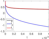
Refer to caption Refer to caption Refer to caption Refer to caption
(a) α=0.25𝛼0.25\alpha=0.25 (b) α=0.5𝛼0.5\alpha=0.5 (c) α=0.75𝛼0.75\alpha=0.75 (d) α=1.00𝛼1.00\alpha=1.00
Figure 1: The Mittag-Leffler function g(t)=Eα,1(λtα)𝑔𝑡subscript𝐸𝛼1𝜆superscript𝑡𝛼g(t)=E_{\alpha,1}(-\lambda t^{\alpha}) and the fractional polynomial approximation fpsubscript𝑓𝑝f_{p} and rational approximation frsubscript𝑓𝑟f_{r} for Example 4.1(i).
Refer to caption Refer to caption Refer to caption Refer to caption
(a) 𝜶=(0.2,0.3)𝜶0.20.3\boldsymbol{\alpha}=(0.2,0.3) (b) 𝜶=(0.2,0.5)𝜶0.20.5\boldsymbol{\alpha}=(0.2,0.5) (c) 𝜶=(0.2,0.7)𝜶0.20.7\boldsymbol{\alpha}=(0.2,0.7) (d) 𝜶=(0.2,0.9)𝜶0.20.9\boldsymbol{\alpha}=(0.2,0.9)
Figure 2: The multinomial Mittag-Leffler function g(t)=1λtα2E(α2,α2α1),1+α2(λtα2,r1tα2α1)𝑔𝑡1𝜆superscript𝑡subscript𝛼2subscript𝐸subscript𝛼2subscript𝛼2subscript𝛼11subscript𝛼2𝜆superscript𝑡subscript𝛼2subscript𝑟1superscript𝑡subscript𝛼2subscript𝛼1g(t)=1-\lambda t^{\alpha_{2}}E_{(\alpha_{2},\alpha_{2}-\alpha_{1}),1+\alpha_{2}}(-\lambda t^{\alpha_{2}},-r_{1}t^{\alpha_{2}-\alpha_{1}}) and the fractional polynomial approximation fpsubscript𝑓𝑝f_{p} and rational approximation frsubscript𝑓𝑟f_{r} for Example 4.1(ii) with r1=0.5subscript𝑟10.5r_{1}=0.5.

Next we present results for numerical recovery of the orders for Example 4.1. The numerical results are presented in Tables 1 and 2 for cases (i) and (ii), respectively. It is observed that for a fixed α=0.7𝛼0.7\alpha=0.7, the recovered α𝛼\alpha represents a very accurate approximation to the exact one, when the time horizon T0subscript𝑇0T_{0} is sufficiently close to zero, and then both models fpsubscript𝑓𝑝f_{p} and frsubscript𝑓𝑟f_{r} have comparable accuracy. However, when T0subscript𝑇0T_{0} increases, the results by the model frsubscript𝑓𝑟f_{r} is much more accurate than that by the model fpsubscript𝑓𝑝f_{p}, which agrees with the preceding observation that frsubscript𝑓𝑟f_{r} is more broadly valid as an approximation to the target function g(t)𝑔𝑡g(t). Meanwhile, when T0subscript𝑇0T_{0} is fixed at 1e-6, the accuracy of the recovered order α𝛼\alpha deteriorates steadily as the true α𝛼\alpha decreases towards zero, for either model function, although the results by the model function frsubscript𝑓𝑟f_{r} are far more accurate, especially when the exact α𝛼\alpha is small. This can be attributed to the behavior of Eα,1(λtα)subscript𝐸𝛼1𝜆superscript𝑡𝛼E_{\alpha,1}(-\lambda t^{\alpha}): at small α𝛼\alpha, Eα,1(λtα)subscript𝐸𝛼1𝜆superscript𝑡𝛼E_{\alpha,1}(-\lambda t^{\alpha}) reaches a quasi-steady state very rapidly, cf. Fig. 1(a), and the fractional polynomial model fpsubscript𝑓𝑝f_{p} fails to accurately capture the behavior, whereas the rational model frsubscript𝑓𝑟f_{r} does so more closely.

Table 1: Numerical results for Example 4.1(i), λ=π2+11.0870𝜆superscript𝜋211.0870\lambda=\pi^{2}+1\approx 1.0870, and the algorithm L-BFGS-B is always initialized to α=0.5𝛼0.5\alpha=0.5, and c𝑐c by the standard linear least-squares method. (a) Fixed α=0.7𝛼0.7\alpha=0.7, recovered with different T0subscript𝑇0T_{0}, and (b) recovered with T0=subscript𝑇0absentT_{0}=1e-6, for different α𝛼\alpha.
fpsubscript𝑓𝑝f_{p} frsubscript𝑓𝑟f_{r}
T0subscript𝑇0T_{0} α𝛼\alpha λ𝜆\lambda α𝛼\alpha λ𝜆\lambda
1e-7 0.6993 1.074e1 0.6995 1.078e1
1e-6 0.6998 1.083e1 0.7001 1.088e1
1e-5 0.6989 1.071e1 0.7005 1.095e1
1e-4 0.6947 1.022e1 0.7026 1.121e1
1e-3 0.6742 8.532e0 0.7129 1.228e1
1e-2 0.5856 4.779e0 0.7570 1.648e1
1e-1 0.3455 1.660e0 0.8563 2.690e1
(a)
fpsubscript𝑓𝑝f_{p} frsubscript𝑓𝑟f_{r}
α𝛼\alpha α𝛼\alpha λ𝜆\lambda α𝛼\alpha λ𝜆\lambda
0.30 0.2669 5.916e0 0.3034 1.157e1
0.40 0.3891 9.008e0 0.4019 1.124e1
0.50 0.4969 1.032e1 0.5008 1.102e1
0.60 0.5991 1.072e1 0.6003 1.092e1
0.70 0.6998 1.083e1 0.7001 1.088e1
0.80 0.7995 1.079e1 0.7990 1.072e1
0.90 0.8937 9.906e0 0.8909 9.521e0
(b)
Table 2: Numerical results for Example 4.1(ii), λ=π2+11.0870𝜆superscript𝜋211.0870\lambda=\pi^{2}+1\approx 1.0870, and the algorithm L-BFGS-B, and the corresponding c𝑐c by the standard linear least-squares method.
fpsubscript𝑓𝑝f_{p} frsubscript𝑓𝑟f_{r}
T0subscript𝑇0T_{0} α1subscript𝛼1\alpha_{1} α2subscript𝛼2\alpha_{2} λ𝜆\lambda r1subscript𝑟1r_{1} α1subscript𝛼1\alpha_{1} α2subscript𝛼2\alpha_{2} λ𝜆\lambda r1subscript𝑟1r_{1}
1e-7 0.5971 0.8985 1.056e1 0 0.5971 0.8985 1.056e1 0
1e-6 0.5943 0.8972 1.032e1 5.49e-12 0.5944 0.8972 1.033e1 6.61e-13
1e-5 0.5887 0.8943 9.938e0 1.04e-11 0.5890 0.8945 9.963e0 1.53e-11
1e-4 0.5766 0.8883 9.284e0 1.59e-9 0.5794 0.8897 9.432e0 1.25e-09
1e-3 0.4227 0.8955 1.015e1 2.08e0 0.5844 0.8922 9.830e0 3.36e-01
1e-2 0.3530 0.8931 9.860e0 2.82e0 0.5788 0.8894 9.220e0 0
(a) 𝜶=(0.6,0.9)𝜶0.60.9\boldsymbol{\alpha}=(0.6,0.9), L-BFGS-B initialized to 𝜶=(0.4,0.8)𝜶0.40.8\boldsymbol{\alpha}=(0.4,0.8)
fpsubscript𝑓𝑝f_{p} frsubscript𝑓𝑟f_{r}
T0subscript𝑇0T_{0} α1subscript𝛼1\alpha_{1} α2subscript𝛼2\alpha_{2} λ𝜆\lambda r1subscript𝑟1r_{1} α1subscript𝛼1\alpha_{1} α2subscript𝛼2\alpha_{2} λ𝜆\lambda r1subscript𝑟1r_{1}
1e-7 0.3889 0.6944 9.616e0 2.28e-12 0.3890 0.6945 9.626e0 5.67e-11
1e-6 0.3824 0.6912 9.129e0 2.41e-11 0.3830 0.6915 9.174e0 5.53e-11
1e-5 0.3713 0.6856 8.466e0 1.03e-9 0.3742 0.6871 8.639e0 8.70e-10
1e-4 0.3914 0.6959 9.954e0 1.50e0 0.5870 0.7010 1.160e1 4.71e-1
1e-3 0.2804 0.6906 9.156e0 2.60e0 0.3625 0.6803 8.051e0 9.89e-2
1e-2 0.5378 0.7315 1.633e1 1.41e0 -0.5278 0.6860 8.261e0 0
(b) 𝜶=(0.5,0.7)𝜶0.50.7\boldsymbol{\alpha}=(0.5,0.7), L-BFGS-B initialized to 𝜶=(0.2,0.6)𝜶0.20.6\boldsymbol{\alpha}=(0.2,0.6)

The numerical results for the two term case in Example 4.1(ii) are summarized in Table 2. It is observed that with proper initialization, the method does recover the orders (α1,α2)subscript𝛼1subscript𝛼2(\alpha_{1},\alpha_{2}) to a reasonable accuracy, for a wide range of the time horizon T0subscript𝑇0T_{0}, with the accuracy of α2subscript𝛼2\alpha_{2} being higher than that of α1subscript𝛼1\alpha_{1}. The latter can be attributed to the asymptotic expansion: the term involving α2subscript𝛼2\alpha_{2} is dominating in the expansion and much easier to estimate than the remaining terms. Indeed, if T0subscript𝑇0T_{0} is sufficiently small, all other terms are essentially negligible, comparing the results in Figs. 1 and 2, and consequently, the order α1subscript𝛼1\alpha_{1} and the weight r1subscript𝑟1r_{1} cannot be estimated reliably at all. This can also been seen from the following slightly more refined expansion in fractional polynomials:

1λtα2E(α2,α2α1),1+α2(λtα2,r1tα2α1)=fp(t)+λ2t2α2Γ(2α2+1)+𝒪(t3α2α1).1𝜆superscript𝑡subscript𝛼2subscript𝐸subscript𝛼2subscript𝛼2subscript𝛼11subscript𝛼2𝜆superscript𝑡subscript𝛼2subscript𝑟1superscript𝑡subscript𝛼2subscript𝛼1subscript𝑓𝑝𝑡superscript𝜆2superscript𝑡2subscript𝛼2Γ2subscript𝛼21𝒪superscript𝑡3subscript𝛼2subscript𝛼1\displaystyle 1-\lambda t^{\alpha_{2}}E_{(\alpha_{2},\alpha_{2}-\alpha_{1}),1+\alpha_{2}}(-\lambda t^{\alpha_{2}},-r_{1}t^{\alpha_{2}-\alpha_{1}})=f_{p}(t)+\lambda^{2}\frac{t^{2\alpha_{2}}}{\Gamma(2\alpha_{2}+1)}+\mathcal{O}(t^{3\alpha_{2}-\alpha_{1}}).

This clearly shows the potential pitfalls in the order recovery: the next term can have comparable magnitude with the last term fpsubscript𝑓𝑝f_{p} when α1subscript𝛼1\alpha_{1} is close to zero, and the nonlinear procedure attempts to approximate it with the leading terms, thereby significantly affecting the recovery accuracy. The accuracy of the recovered λ𝜆\lambda is also reasonable, except for fairly large T0subscript𝑇0T_{0}. However, the accuracy of r1subscript𝑟1r_{1} is poor in all cases, due to the aforementioned reasons. Also as the orders decrease, it is becoming increasingly more challenging for the numerical recovery, which agrees with the empirical observation from Example 4.1(i), cf. Table 2(b). This is attributed to the rapid decay near t=0𝑡0t=0 so that the model functions are not accurate. These results partly confirm the assertion in Theorem 1.2: the recovery is indeed possible, however, numerically this can still be a big challenge, depending on the magnitude of the sought-for orders. It is of great interest to develop further remedies to tackle the numerical issues.

The next example illustrates the feasibility of the approach in the general setting.

Example 4.2.

The domain Ω=(0,1)2Ωsuperscript012\Omega=(0,1)^{2}, Au=Δu𝐴𝑢Δ𝑢Au=-\Delta u with zero Neumann boundary condition, with a two-term model with 0<α1<α2<10subscript𝛼1subscript𝛼210<\alpha_{1}<\alpha_{2}<1 and the corresponding weights r1subscript𝑟1r_{1} and r2=1subscript𝑟21r_{2}=1. The measurement point x0subscript𝑥0x_{0} is the vertex point x0=(0,0)subscript𝑥000x_{0}=(0,0). Consider the following two cases: (i) u0(x1,x2)=cosπx1cosπx2+14(cos2πx1cosπx2+cosπx1cos2πx2)+18cos2πx1cos2πx2subscript𝑢0subscript𝑥1subscript𝑥2𝜋subscript𝑥1𝜋subscript𝑥2142𝜋subscript𝑥1𝜋subscript𝑥2𝜋subscript𝑥12𝜋subscript𝑥2182𝜋subscript𝑥12𝜋subscript𝑥2u_{0}(x_{1},x_{2})=\cos\pi x_{1}\cos\pi x_{2}+\frac{1}{4}(\cos 2\pi x_{1}\cos\pi x_{2}+\cos\pi x_{1}\cos 2\pi x_{2})+\frac{1}{8}\cos 2\pi x_{1}\cos 2\pi x_{2} and f0𝑓0f\equiv 0 and (ii) u00subscript𝑢00u_{0}\equiv 0 and f(x1,x2,t)=cosπx1cosπx2+12(cos2πx1cosπx2+cosπx1cos2πx2)+14(cos3πx1cosπx2+cosπx1cos3πx2)𝑓subscript𝑥1subscript𝑥2𝑡𝜋subscript𝑥1𝜋subscript𝑥2122𝜋subscript𝑥1𝜋subscript𝑥2𝜋subscript𝑥12𝜋subscript𝑥2143𝜋subscript𝑥1𝜋subscript𝑥2𝜋subscript𝑥13𝜋subscript𝑥2f(x_{1},x_{2},t)=\cos\pi x_{1}\cos\pi x_{2}+\frac{1}{2}(\cos 2\pi x_{1}\cos\pi x_{2}+\cos\pi x_{1}\cos 2\pi x_{2})+\frac{1}{4}(\cos 3\pi x_{1}\cos\pi x_{2}+\cos\pi x_{1}\cos 3\pi x_{2}). The goal is to recover the following quantities: 𝛂𝛂\boldsymbol{\alpha}, r1subscript𝑟1r_{1} and Au(x0)𝐴𝑢subscript𝑥0Au(x_{0}) or f(x0)𝑓subscript𝑥0f(x_{0}) for cases (i) and (ii), respectively, from the data g(t)=u(x0,t)𝑔𝑡𝑢subscript𝑥0𝑡g(t)=u(x_{0},t).

Note that for this example, the data g(t)=u(x0,t)𝑔𝑡𝑢subscript𝑥0𝑡g(t)=u(x_{0},t) can be generated using the standard Galerkin finite element method in space and convolution quadrature in time [10]. Below we employ series expansion using the multinomial Mittag-Leffler function, cf. Remark 4.1, so as to minimize the discretization errors, and like before, it is evaluated by means of series summation (truncated at k=100𝑘100k=100). In case (ii), the model functions fpsubscript𝑓𝑝f_{p} and frsubscript𝑓𝑟f_{r} are given respectively by

fp(t)subscript𝑓𝑝𝑡\displaystyle f_{p}(t) =f(x0)(tα2Γ(α2+1)r1t2α2α1Γ(2α2α1+1)),absent𝑓subscript𝑥0superscript𝑡subscript𝛼2Γsubscript𝛼21subscript𝑟1superscript𝑡2subscript𝛼2subscript𝛼1Γ2subscript𝛼2subscript𝛼11\displaystyle=f(x_{0})\Big{(}\frac{t^{\alpha_{2}}}{\Gamma(\alpha_{2}+1)}-\frac{r_{1}t^{2\alpha_{2}-\alpha_{1}}}{\Gamma(2\alpha_{2}-\alpha_{1}+1)}\Big{)},
fr(t)subscript𝑓𝑟𝑡\displaystyle f_{r}(t) =f(x0)(111+tα2Γ(α2+1)r1t2α2α1Γ(2α2α1+1)),absent𝑓subscript𝑥0111superscript𝑡subscript𝛼2Γsubscript𝛼21subscript𝑟1superscript𝑡2subscript𝛼2subscript𝛼1Γ2subscript𝛼2subscript𝛼11\displaystyle=f(x_{0})\Big{(}1-\frac{1}{1+\frac{t^{\alpha_{2}}}{\Gamma(\alpha_{2}+1)}-\frac{r_{1}t^{2\alpha_{2}-\alpha_{1}}}{\Gamma(2\alpha_{2}-\alpha_{1}+1)}}\Big{)},

where the latter follows by direct analogy. The numerical results are given in Table 3. The observations from Example 4.1 remain largely valid. In both cases (i) and (ii), the orders can be accurately recovered, provided that the time horizon T0subscript𝑇0T_{0} is sufficiently small (so that the model functions are accurate approximations). The accuracy of the two models are largely comparable to each other in either case, and deteriorates steadily as T0subscript𝑇0T_{0} increases. Also the accuracy of the recovered Au(x0)=𝐴𝑢subscript𝑥0absentAu(x_{0})=5.428e1 and f(x0)=2.500𝑓subscript𝑥02.500f(x_{0})=2.500 is fair. Just as expected, the accuracy of the estimated r1subscript𝑟1r_{1} is poor in all cases, irrespective of the time horizon T0subscript𝑇0T_{0}, which also agrees with preceding observations. These numerical experiments not only confirm the possibility of uniquely recovery as indicated by Theorems 1.1 and 1.2, but also illustrate the pitfalls in developing practical recovery schemes.

Table 3: Numerical results for Example 4.2, and the algorithm L-BFGS-B, and the corresponding c𝑐c by the standard linear least-squares method.
fpsubscript𝑓𝑝f_{p} frsubscript𝑓𝑟f_{r}
T0subscript𝑇0T_{0} α1subscript𝛼1\alpha_{1} α2subscript𝛼2\alpha_{2} Au(x0)𝐴𝑢subscript𝑥0Au(x_{0}) r1subscript𝑟1r_{1} α1subscript𝛼1\alpha_{1} α2subscript𝛼2\alpha_{2} Au(x0)𝐴𝑢subscript𝑥0Au(x_{0}) r1subscript𝑟1r_{1}
1e-8 0.4992 0.7996 5.380e1 0 0.4992 0.7996 5.381e1 0
1e-7 0.4984 0.7992 5.340e1 0 0.4985 0.7992 5.344e1 0
1e-6 0.4965 0.7983 5.261e1 0 0.4971 0.7985 5.284e1 0
1e-5 0.4913 0.7956 5.079e1 0 0.4946 0.7973 5.196e1 0
1e-4 0.4716 0.7858 4.551e1 0 0.4920 0.7960 5.118e1 0
(a) 𝜶=(0.5,0.8)𝜶0.50.8\boldsymbol{\alpha}=(0.5,0.8), L-BFGS-B initialized to 𝜶=(0.3,0.7)𝜶0.30.7\boldsymbol{\alpha}=(0.3,0.7)
fpsubscript𝑓𝑝f_{p} frsubscript𝑓𝑟f_{r}
T0subscript𝑇0T_{0} α1subscript𝛼1\alpha_{1} α2subscript𝛼2\alpha_{2} f(x0)𝑓subscript𝑥0f(x_{0}) r1subscript𝑟1r_{1} α1subscript𝛼1\alpha_{1} α2subscript𝛼2\alpha_{2} f(x0)𝑓subscript𝑥0f(x_{0}) r1subscript𝑟1r_{1}
1e-8 0.4964 0.6982 2.393 0 0.4964 0.6982 2.393 1.29e-10
1e-7 0.4941 0.6970 2.343 1.27e-10 0.4941 0.6970 2.343 9.13e-10
1e-6 0.5023 0.7015 2.583 6.41e-1 0.4896 0.6948 2.261 2.11e-9
1e-5 0.2083 0.6974 2.366 8.56e0 0.2167 0.6975 2.367 7.54e0
1e-4 0.1669 0.6969 2.343 1.23e1 0.1668 0.6967 2.337 1.16e1
(b) 𝜶=(0.5,0.7)𝜶0.50.7\boldsymbol{\alpha}=(0.5,0.7), L-BFGS-B initialized to 𝜶=(0.3,0.6)𝜶0.30.6\boldsymbol{\alpha}=(0.3,0.6)

5 Conclusions

In this work we have proved the unique recovery of multiple fractional orders and the associated weights in a multi-term time-fractional diffusion model from the observation at one point on the boundary, based on the asymptotics of the solution at small time and the time analyticity of the solution. We have also discussed the numerical recovery based on asymptotic expansion / rational approximation, and demonstrated the feasibility of the least-squares approach for recovering the highest order and the weight.

It is of much interest to study related inverse problems for more complex anomalous diffusion models, e.g., distributed-order or variable-order. It is unclear whether the one-point observation is sufficient for the unique recovery of the order distribution in these models, but a partial determination, e.g., support in the distributed order, might be possible. Further, it remains an outstanding challenge to develop stable and accurate numerical procedures for recovering all fractional orders, by properly overcoming the difficulty with unknown media.

References

  • [1] S. Alimov and R. Ashurov. Inverse problem of determining an order of the Caputo time-fractional derivative for a subdiffusion equation. J. Inverse Ill-Posed Probl., 28(5):651–658, 2020.
  • [2] R. H. Byrd, P. Lu, J. Nocedal, and C. Y. Zhu. A limited memory algorithm for bound constrained optimization. SIAM J. Sci. Comput., 16(5):1190–1208, 1995.
  • [3] J. Cheng, J. Nakagawa, M. Yamamoto, and T. Yamazaki. Uniqueness in an inverse problem for a one-dimensional fractional diffusion equation. Inverse Problems, 25(11):115002, 16, 2009.
  • [4] W. Feller. An Introduction to Probability Theory and Its Applications, Volume II. John Wiley & Sons, New York, 1970.
  • [5] P. Grisvard. Elliptic Problems in Nonsmooth Domains. Pitman, Boston, MA, 1985.
  • [6] Y. Hatano, J. Nakagawa, S. Wang, and M. Yamamoto. Determination of order in fractional diffusion equation. J. Math-for-Ind., 5A:51–57, 2013.
  • [7] K. Ito and B. Jin. Inverse Problems: Tikhonov Theory and Algorithms. World Scientific, Hackensack, NJ, 2015.
  • [8] B. Jin. Fractional Differential Equations. Springer-Nature, Switzerland, 2021.
  • [9] B. Jin and Y. Kian. Recovery of the order of derivation for fractional diffusion equations in an unknown medium. Preprint, arXiv:2101.09165, 2021.
  • [10] B. Jin, R. Lazarov, and Z. Zhou. Two fully discrete schemes for fractional diffusion and diffusion-wave equations with nonsmooth data. SIAM J. Sci. Comput., 38(1):A146–A170, 2016.
  • [11] B. Jin, B. Li, and Z. Zhou. Numerical analysis of nonlinear subdiffusion equations. SIAM J. Numer. Anal., 56(1):1–23, 2018.
  • [12] Y. Kian. Simultaneous determination of coefficients and internal source of a diffusion equation from a single measurement. Preprint, arXiv:2007.08947, 2020.
  • [13] Y. Kian, E. Soccorsi, Q. Xue, and M. Yamamoto. Identification of time-varying source term in time-fractional diffusion equations. Commun. Math. Sci., page in press, 2021.
  • [14] Y. Kian, E. Soccorsi, and M. Yamamoto. On time-fractional diffusion equations with space-dependent variable order. Ann. Henri Poincaré, 19(12):3855–3881, 2018.
  • [15] A. A. Kilbas, H. M. Srivastava, and J. J. Trujillo. Theory and Applications of Fractional Differential Equations. Elsevier Science B.V., Amsterdam, 2006.
  • [16] Z. Li, O. Y. Imanuvilov, and M. Yamamoto. Uniqueness in inverse boundary value problems for fractional diffusion equations. Inverse Problems, 32(1):015004, 16, 2016.
  • [17] Z. Li, Y. Kian, and E. Soccorsi. Initial-boundary value problem for distributed order time-fractional diffusion equations. Asymptot. Anal., 115(1-2):95–126, 2019.
  • [18] Z. Li, Y. Liu, and M. Yamamoto. Initial-boundary value problems for multi-term time-fractional diffusion equations with positive constant coefficients. Appl. Math. Comput., 257:381–397, 2015.
  • [19] Z. Li, Y. Liu, and M. Yamamoto. Inverse problems of determining parameters of the fractional partial differential equations. In Handbook of Fractional Calculus with Applications. Vol. 2, pages 431–442. De Gruyter, Berlin, 2019.
  • [20] Z. Li and M. Yamamoto. Uniqueness for inverse problems of determining orders of multi-term time-fractional derivatives of diffusion equation. Appl. Anal., 94(3):570–579, 2015.
  • [21] Z. Li and Z. Zhang. Unique determination of fractional order and source term in a fractional diffusion equation from sparse boundary data. Inverse Problems, 36(11):115013, 20, 2020.
  • [22] K. Liao and T. Wei. Identifying a fractional order and a space source term in a time-fractional diffusion-wave equation simultaneously. Inverse Problems, 35(11):115002, 23, 2019.
  • [23] Y. Luchko. Initial-boundary problems for the generalized multi-term time-fractional diffusion equation. J. Math. Anal. Appl., 374(2):538–548, 2011.
  • [24] Y. Luchko and R. Gorenflo. An operational method for solving fractional differential equations with the Caputo derivatives. Acta Math. Vietnam., 24(2):207–233, 1999.
  • [25] F. Mainardi. On some properties of the Mittag-Leffler function Eα(tα)subscript𝐸𝛼superscript𝑡𝛼E_{\alpha}(-t^{\alpha}), completely monotone for t>0𝑡0t>0 with 0<α<10𝛼10<\alpha<1. Discrete Contin. Dyn. Syst. Ser. B, 19(7):2267–2278, 2014.
  • [26] R. Metzler and J. Klafter. The random walk’s guide to anomalous diffusion: a fractional dynamics approach. Phys. Rep., 339(1):77, 2000.
  • [27] R. Metzler, J. Klafter, and I. M. Sokolov. Anomalous transport in external fields: continuous time random walks and fractional diffusion equations extended. Phys. Rev. E, 58(2):1621–1633, 1998.
  • [28] P. Royston and W. Sauerbrei. Multivariable Model-Building. John Wiley & Sons, Ltd., Chichester, 2008.
  • [29] W. Rudin. Real and Complex Analysis. McGraw Hill, 1987.
  • [30] R. Schumer, D. A. Benson, M. M. Meerschaert, and B. Baeumer. Fractal mobile/immobile solute transport. Water Res. Research, 39(10):1296, 13 pp., 2003.
  • [31] H. Seybold and R. Hilfer. Numerical algorithm for calculating the generalized Mittag-Leffler function. SIAM J. Numer. Anal., 47(1):69–88, 2008/09.
  • [32] T. Simon. Comparing Fréchet and positive stable laws. Electron. J. Probab., 19:no. 16, 25, 2014.
  • [33] L. Sun, Y. S. Li, and Y. Zhang. Simultaneous inversion of the potential term and the fractional orders in a multi-term time-fractional diffusion equation. Inverse Problems, 37(5):055007, 2021.
  • [34] E. C. Titchmarsh. The zeros of certain integral functions. Proc. London Math. Soc. (2), 25:283–302, 1926.
  • [35] V. Vergara and R. Zacher. Optimal decay estimates for time-fractional and other nonlocal subdiffusion equations via energy methods. SIAM J. Math. Anal., 47(1):210–239, 2015.
  • [36] H. Weyl. Das asymptotische Verteilungsgesetz der Eigenwerte linearer partieller Differentialgleichungen (mit einer Anwendung auf die Theorie der Hohlraumstrahlung). Math. Ann., 71(4):441–479, 1912.
  • [37] M. Yamamoto. Uniqueness for inverse problem of determining fractional orders for time-fractional advection-diffusion equations. Preprint, arXiv:2103.15166, 2021.