Quantum critical systems with dissipative boundaries

Abstract

We study the effects of dissipative boundaries in many-body systems at continuous quantum transitions, when the parameters of the Hamiltonian driving the unitary dynamics are close to their critical values. As paradigmatic models, we consider fermionic wires subject to dissipative interactions at the boundaries, associated with pumping or loss of particles. They are induced by couplings with a Markovian baths, so that the evolution of the system density matrix can be described by a Lindblad master equation. We study the quantum evolution arising from variations of the Hamiltonian and dissipation parameters, starting at $t=0$ from the ground state of the Hamiltonian at, or close to, the critical point. Two different dynamic regimes emerge: (i) an early-time regime for times $t\sim L$, where the competition between coherent and incoherent drivings develops a dynamic finite-size scaling, obtained by extending the scaling framework describing the coherent critical dynamics of the closed system, to allow for the boundary dissipation; (ii) a large-time regime for $t\sim L^{3}$ whose dynamic scaling describes the late quantum evolution leading to the $t\to\infty$ stationary states.

I Introduction

The out-of-equilibrium dynamics of quantum many-body systems has been much investigated in the recent years. The recent progress in quantum technologies has also enabled experimental studies in the presence of dissipation, either associated with unavoidable incoherent mechanisms, or with suitably engineered system-bath couplings. Dissipative mechanisms arising from the interaction with an environment HTK-12 ; MDPZ-12 ; CC-13 ; AKM-14 may lead to the emergence of new collective phenomena, such as novel quantum phases and phase transitions driven by dissipation Hartmann-16 ; NA-17 ; MBBC-18 ; LCF-19 ; SRN-19 , and the emergence of dynamic scaling behaviors in the low-dissipative regime of many-body systems at quantum transitions RV-21-rev ; YMZ-14 ; YLC-16 ; NRV-19 ; RV-19 ; RV-20 .

Figure 1: Sketch of a one-dimensional lattice system with boundary dissipation, arising from the interactions with two baths at the boundary sites, which may be of different nature. In this paper we focus on the effects of boundary dissipative interactions when the quantum system is close to a bulk quantum transition, and therefore is characterized by quantum critical correlations.

In this paper we address the effects of dissipative boundaries in many-body systems, such as the set up sketched in Fig. 1, at continuous quantum transitions (CQTs), when the parameters of the Hamiltonian driving the unitary dynamics are close to their critical values.

Some issues related to the effects of dissipation on quantum systems at CQTs have been already investigated YMZ-14 ; YLC-16 ; NRV-19 ; RV-19 ; RV-20 . We recall that isolated many-body systems at CQTs develop dynamic scaling behaviors, characterized by a diverging length scale $\xi$, and a vanishing gap $\Delta$, as $\Delta\sim\xi^{-z}$ where $z$ is the universal dynamic exponent SGCS-97 ; Sachdev-book . The dissipative mechanisms considered in Refs. YMZ-14, ; YLC-16, ; NRV-19, ; RV-19, ; RV-20, were modeled by Lindblad master equations governing the time evolution of the density matrix. A dynamic scaling behavior emerges even in the presence of dissipation, whose main features are controlled by the universality class of the CQT. However, such a dynamic scaling limit requires a particular tuning of the dissipative interactions, whose dissipative rate $u$ must scale as $u\sim\Delta\sim\xi^{-z}$. These studies have been also extended to first-order quantum transitions DRV-20 , where a peculiar dynamic scaling emerges as well, which appears more complex due to the strong sensitivity of first-order transitions to the boundary conditions CNPV-14 .

The above-mentioned works have focused on dissipative mechanisms arising from homogenous couplings with external baths, involving the bulk of the system, such as those sketched in Fig. 2. In this paper we consider a different problem, focussing on critical systems subject to dissipative interactions at the boundaries only, arising from environmental baths that can only interact with the boundaries of the system, as sketched in Fig. 1. We investigate the impact of boundary dissipation to the quantum critical behavior of systems when it is closed to its CQT, i.e. when the Hamiltonian parameters are tuned to a quantum critical point. We want to understand whether boundary dissipations maintain the system within a critical regime, or they make the system depart from criticality, whether their effects can be casted within a dynamic scaling framework as in the case of homogenous dissipative mechanisms.

Figure 2: Sketch of a one-dimensional lattice system in which the sites are homogeneously coupled to independent and equal baths ${\mathcal{B}}$, whose effect is to introduce local incoherent mechanisms. Therefore the dissipative mechanism is homogenous, and translation invariance is preserved (of course if translation invariance is satisfied by the Hamiltonian of the quantum system, and there are no boundaries, for example assuming periodic or antiperiodic boundary conditions). The effects of such homogeneous local dissipation at quantum transitions, modeled by corresponding Lindblad equations, have been analyzed in Refs. NRV-19, ; RV-19, ; RV-20, .

We model the dissipative interaction with the environment by Lindblad master equations for the density matrix of the system BP-book ; RH-book ,

$${\partial\rho\over\partial t}={\cal L}[\rho]:=-{i\over\hslash}\,[\hat{H},\rho]+{\mathbb{D}}[\rho]\,,$$ (1)

where the generator ${\cal L}$ of the dynamics is called a Liouvillian or a Lindbladian, the first term in the r.h.s. provides the coherent Hamiltonian driving, while the second term accounts for the dissipative coupling to the environment. In the case of systems weakly coupled to Markovian baths, the trace-preserving superoperator ${\mathbb{D}}[\rho]$ can be generally written as a sum of terms associated with the various sources in contact with the system Lindblad-76 ; GKS-76 , i.e.

$${\mathbb{D}}[\rho] = \sum_{b}w_{b}\,{\mathbb{D}}_{b}[\rho]\,,$$ (2)

$${\mathbb{D}}_{b}[\rho] = \hat{L}_{b}^{\phantom{\dagger}}\rho\hat{L}_{b}^{\dagger}-\tfrac{1}{2}\big{(}\rho\,\hat{L}_{b}^{\dagger}\hat{L}_{b}^{\phantom{\dagger}}+\hat{L}_{b}^{\dagger}\hat{L}_{b}^{\phantom{\dagger}}\rho\big{)}\,,$$

where $\hat{L}_{b}$ is the Lindblad jump operator describing the coupling between the system and the bath labeled by $b$, and $w_{b}$ are parameters controlling the strength or dissipative rate of the corresponding dissipative interaction. The form of the Lindblad operators depends on the nature of the dissipation arising from the interaction with the bath. In quantum optical implementations, the conditions leading to the Lindblad framework are typically satisfied SBD-16 ; DR-21 .

As a paradigmatic model, we consider the fermionic Kitaev wire Kitaev-01 , which undergoes a CQT belonging to the two-dimensional Ising universality class. This choice allows us to perform numerical computations for relatively large systems, thus accurate checks of the dynamic scaling behaviors that we put forward. We study the dynamic behavior close to the CQT, in the presence of dissipation due to local incoherent particle pumping or loss at the boundaries. We study the quantum evolution driven by the Lindbladian master equation (1), arising from variations of the Hamiltonian and dissipation parameters, starting at the initial time $t=0$ from the ground state of the Hamiltonian close to the critical point. We show that the quantum evolution of fermionic wires of size $L$ is characterized by two distinct dynamic regimes. We observe an early-time regime for $t\sim L$, where the competition between coherent and incoherent drivings develop a dynamic finite-size scaling (FSS), obtained by extending the dynamic FSS framework describing the out-of-equilibrium critical dynamics of the closed system RV-21-rev , to allow for the boundary dissipation. Then, at larger times, $t\sim L^{3}$, a different regime sets in, whose dynamic scaling describes the late quantum evolution leading to the $t\to\infty$ stationary states. The above scenario is observed keeping the boundary dissipative rate fixed, i.e. no tuning of the dissipative rate turns out to be necessary, unlike the case of homogenous dissipative mechanisms.

We finally mention that some issues concerning localized dissipative interactions with the environment have been already discussed in the literature, see e.g. Refs. PP-08, ; Prosen-08, ; BGZ-14, ; Znidaric-15, ; VCG-18, ; FCKD-19, ; TFDM-19, ; BMA-19, ; KMS-19, ; SK-20, ; WSDK-20, ; FMKCD-20, ; Rossini-etal-20, ; AC-21, , and in particular the case of quantum Ising chains with dissipative interactions at the ends of the chain PP-08 ; Prosen-08 ; BGZ-14 ; Znidaric-15 ; VCG-18 ; SK-20 , mainly focussing on the approach to the asymptotic large-time stationary states. In this paper we are interested in the whole dynamic behavior from the early-time regime to the large-time regime leading to the stationary states, addressing in particular the interplay with the finite size of the system.

The paper is organized as follows. In Sec. II we present the paradigmatic fermionic Kitaev wire and the boundary dissipative interactions with the environment that we consider in our study; moreover we outline the dynamic protocol that we consider to address the interplay between coherent Hamiltonian and incoherent boundary dissipative drivings. In Sec. III we introduce the dynamic FSS framework that allows us to describe the early-time regime of the out-of-equilibrium quantum evolution associated with the protocol that we consider. In Sec. IV we present our numerical results, showing the emergence of different early-time and large-time regimes, characterized by different time scales. Finally in Sec. V we summarize and draw our conclusions. In App. A we report some details of the numerical computations.

II Fermionic wires subject to boundary dissipation

II.1 The Kitaev model

We consider fermionic quantum wires of $L$ sites, whose quantum unitary dynamics is driven by the Kitaev Hamiltonian Kitaev-01

$$\hat{H}_{\rm K}=-t\sum_{x=1}^{L-1}\big{(}\hat{c}_{x}^{\dagger}\hat{c}_{x+1}^{\phantom{\dagger}}+\delta\,\hat{c}_{x}^{\dagger}\hat{c}_{x+1}^{\dagger}+{\rm h.c.}\big{)}-\mu\sum_{x=1}^{L}\hat{n}_{x}\,,$$ (3)

where $\hat{c}_{x}$ is the fermionic annihilation operator on the $x^{\rm th}$ site of the chain, $\hat{n}_{x}\equiv\hat{c}_{x}^{\dagger}\hat{c}_{x}^{\phantom{\dagger}}$ is the density operator, and $\delta>0$. Note that the Hamiltonian (3) describe a chain with open boundary conditions. In the following we set $\hslash=1$, $t=1$ as the energy scale, and $\delta=1$.

The Hamiltonian (3) can be mapped into a spin-1/2 XY chain, by means of a Jordan-Wigner transformation, see, e.g., Ref. Sachdev-book, . Fixing $\delta=1$, the corresponding spin model is the quantum Ising chain

$$\hat{H}_{\rm Is}=-\sum_{x=1}^{L-1}\hat{\sigma}^{(1)}_{x}\hat{\sigma}^{(1)}_{x+1}-g\,\sum_{x=1}^{L}\hat{\sigma}^{(3)}_{x}\,,$$ (4)

$\hat{\sigma}^{(k)}_{x}$ being the Pauli matrices and $g=-\mu/2$. In the following we prefer to stick with the Kitaev quantum wire, because the boundary dissipation that we consider is more naturally defined for Fermi lattice gases, in terms of particle pumping and loss mechanisms.

The Kitaev model undergoes a CQT at $\mu=\mu_{c}=-2$, independently of $\delta$, between a disordered ($\mu<\mu_{c}$) and an ordered ($|\mu|<|\mu_{c}|$) quantum phase. This transition belongs to the two-dimensional Ising universality class Sachdev-book ; RV-21-rev , characterized by the length-scale critical exponent $\nu=1$, related to the renormalization-group dimension $y_{\mu}=1/\nu=1$ of the Hamiltonian parameter $\mu$ (more precisely of the difference $\bar{\mu}\equiv\mu-\mu_{c}$). This implies that, approaching the critical point, the length scale $\xi$ of the critical quantum fluctuations diverges as $\xi\sim|\bar{\mu}|^{-\nu}$ where $\bar{\mu}\equiv\mu-\mu_{c}$. The dynamic exponent $z=1$ associated with the unitary quantum dynamics can be obtained from the power law $\Delta\sim\xi^{-z}$ of the vanishing gap with increasing $\xi$.

II.2 Boundary dissipative mechanisms

We focus on the dynamic behavior of the Fermi lattice gas (3) close to its CQT, in the presence of boundary dissipation mechanisms as described by the Lindblad Eq. (1). We consider dissipative mechanisms associated with the boundary sites of the chain, as sketched in Fig. 1. Within the Lindblad framework (1), they are described by the dissipator

$${\mathbb{D}}[\rho]=w_{1}{\mathbb{D}}_{1}[\rho]+w_{L}{\mathbb{D}}_{L}[\rho]\,,$$ (5)

$${\mathbb{D}}_{x}[\rho]=\hat{L}_{x}^{\phantom{\dagger}}\rho\hat{L}_{x}^{\dagger}-\tfrac{1}{2}\big{(}\rho\,\hat{L}_{x}^{\dagger}\hat{L}_{x}^{\phantom{\dagger}}+\hat{L}_{x}^{\dagger}\hat{L}_{x}^{\phantom{\dagger}}\rho\big{)}\,,$$

where $\hat{L}_{x}$ denotes the Lindblad operator associated with the system-bath coupling scheme. The strength of the boundary dissipative mechanisms are controlled by the parameters $w_{1}$ and $w_{L}$, which are related to the dissipative rates of the two processes. The Lindblad operators $\hat{L}_{1}$ and $L_{L}$ describe the coupling of the boundary sites with the corresponding baths ${\mathcal{B}}$, see Fig. 1. We consider different dissipation mechanisms at the two ends of the chain, associated with particle losses and pumping, respectively HC-13 ; KMSFR-17 ; Nigro-19 ; NRV-19 :

$$\hat{L}_{{1}}=\hat{c}_{1}\,,\qquad\hat{L}_{{L}}=\hat{c}_{L}^{\dagger}\,.$$ (6)

II.3 The protocol

To address the competition between coherent and boundary dissipative drivings, we study the evolution after a quench of the Hamiltonian parameters and dissipative interactions with the external baths. Analogous protocols have been also considered to study the effects of homogenous dissipative mechanisms preserving translation invariance NRV-19 ; RV-19 ; DRV-20 . The protocol that we consider is as follows.

• The system starts from the ground state $|0,\bar{\mu}_{i}\rangle$ of $\hat{H}_{K}$ for a generic $\bar{\mu}_{i}\equiv\mu_{i}-\mu_{c}$, sufficiently small to stay within the critical regime. Therefore the initial density matrix is given by

  $$\rho_{i}\equiv\rho(t=0)=|0,\bar{\mu}_{i}\rangle\langle 0,\bar{\mu}_{i}|\,.$$ (7)

• The out-of-equilibrium dynamics starts at $t=0$, arising from a sudden quench of the Hamiltonian parameter, from $\bar{\mu}_{i}$ to $\bar{\mu}\equiv\mu-\mu_{c}$, and the simultaneous turning on the dissipative interactions at the boundaries, as described by the boundary dissipator (5), with dissipation parameters $w_{1}$ and $w_{L}$.

• The evolution of the quantum system, and in particular its density matrix, is described by the Lindblad master equation (1).

The time evolution is studied by monitoring a number of observables, such as the particle density

$$D(x,t)={\rm Tr}[\rho(t)\,\hat{n}_{x}]\,,$$ (8)

and the fermionic current

$$J(x,t)={\rm Tr}[\rho(t)\,\hat{j}_{x}]\,,\quad\hat{j}_{x}=i\left(\hat{c}_{x+1}^{\dagger}\hat{c}_{x}^{\phantom{\dagger}}-\hat{c}_{x}^{\dagger}\hat{c}_{x+1}^{\phantom{\dagger}}\right)\,,$$ (9)

where $\rho(t)$ is the time dependent density matrix driven by the Lindblad equation with dissipative boundaries. Moreover, we consider the fixed-time fermionic correlations

$$G_{c}(x,y,t) = {\rm Tr}[\rho(t)(\hat{c}_{x}^{\dagger}\hat{c}_{y}^{\phantom{\dagger}}+\hat{c}_{y}^{\dagger}\hat{c}_{x}^{\phantom{\dagger}})]\,,$$ (10)

$$G_{p}(x,y,t) = {\rm Tr}[\rho(t)(\hat{c}_{x}^{\dagger}\hat{c}_{y}^{\dagger}+\hat{c}_{y}^{\phantom{\dagger}}\hat{c}_{x}^{\phantom{\dagger}})]\,.$$ (11)

Note that translation invariance does not hold due to the boundaries.

III Dynamic scaling behavior in the presence of dissipation

Before presenting the results for the problem addressed in the paper, we briefly review some features of the dynamic scaling framework, which we will exploit to characterize the dynamics of critical systems with dissipative boundaries. This approach was developed in Refs. NRV-19, ; RV-19, ; RV-20, ; DRV-20, , extending the dynamic scaling framework for isolated systems SGCS-97 ; ZDZ-05 ; Polkovnikov-05 ; Dziarmaga-05 ; DOV-09 ; DGP-10 ; GZHF-10 ; CEGS-12 ; KCH-12 ; FDGZ-16 ; PRV-18 ; PRV-18-loc ; v-18 ; RV-19-decoh ; NRV-19-work (see also Ref. RV-21-rev, for a review of results on these issues).

The initial $t=0$ conditions of the observables monitoring the dynamic evolution is simply provided by their expectation values on the ground state $|0,\bar{\mu}_{i}\rangle$ of the many-body Hamiltonian $H_{K}$ at the initial value $\bar{\mu}_{i}$, which can be obtained by using the initial pure-state density matrix $\rho_{i}=|0,\bar{\mu}_{i}\rangle\langle 0,\bar{\mu}_{i}|$ in Eqs. (10) and(11). Close to the quantum transition, i.e. when $|\bar{\mu}_{i}|\ll 1$, they develop asymptotic FSS behaviors SGCS-97 ; CPV-14 ; RV-21-rev . Their scaling behavior is controlled by critical exponents $\nu=y_{\mu}^{-1}=1$ and $z=1$ of the Ising universality class, and by the renormalization-group dimension $y_{c}=1/2$ of the fermionic operators $\hat{c}_{x}$ and $\hat{c}^{\dagger}_{x}$ Sachdev-book ; RV-21-rev . The initial ($t=0$) ground-state fermionic correlations $G_{i,c/p}$ behave as CPV-14

$$G_{i}(x,y,\bar{\mu}_{i},L)=L^{-2y_{c}}\left[{\cal G}_{i}(X,Y,\kappa_{i})+O(L^{-1})\right],\qquad$$ (12)

$$X=x/L\,,\qquad Y=y/L\,,\qquad\kappa_{i}=\bar{\mu}_{i}L^{y_{\mu}}\,,$$ (13)

in the large-$L$ limit keeping $X$, $Y$, and $\kappa_{i}$ fixed. Note that $G_{i,c/p}$, and the corresponding scaling functions ${\cal G}_{i,c/p}$, maintain the separate dependence on both space variables $x$ and $y$, due to the presence of the boundaries. Moreover the presence of boundaries gives also rise to the leading $O(1/L)$ scaling corrections, which are absent in the case of systems without boundaries CPV-14 , such as systems with periodic or antiperiodic boundary conditions. The scaling corrections arising from the leading irrelevant operator at the Ising fixed point are more suppressed for the two-dimensional Ising universality class CCCPV-00 ; CHPV-02 ; CPV-14 , as $L^{-2}$.

The equilibrium (ground-state) FSS behavior of the particle density is more complex, since the leading contribution comes from analytical terms, while the scaling part is subleading. Indeed the equilibrium ground-state particle density, corresponding to the initial condition of the protocol considered behaves as CPV-14

$$D(x,\bar{\mu}_{i},L)\approx D_{\rm reg}(x,\bar{\mu}_{i},L)+L^{-y_{n}}{\cal D}(X,\kappa_{i})\,,\quad$$ (14)

where $y_{n}=d+z-y_{\mu}=1$ is the renormalization-group dimension of the particle density operator. The regular function $D_{\rm reg}$ provides the leading behavior, which arises from short-ranged fluctuations, while the scaling part arising from the critical modes is suppressed by a power $L^{-y_{n}}$. This does not make the particle density particularly effective to highlight phenomena arising from quantum long-range fluctuations. Fermionic correlations, such as those in Eqs. (10) and (11), are more suitable for this purpose. We also mention that the fermionic current $J(x,t)$, cf. Eq. (9), vanishes at equilibrium, thus its initial value is zero.

The equilibrium ground-state FSS can be extended to address out-of-equilibrium coherent evolutions, for example arising from instantaneous quenches of the Hamiltonian parameter from $\bar{\mu}_{i}$ to $\bar{\mu}$, starting from the ground state associated with $\bar{\mu}_{i}$ at $t=0$. This requires the introduction of a further scaling variable associated with time, given by $\theta=tL^{-z}\sim t\Delta_{L}$, where $\Delta_{L}\sim L^{-z}$ is the gap (i.e., the difference between the lowest energy levels) of the critical Hamiltonian $H_{K}$ at $\bar{\mu}=0$. For open boundary conditions, Pfeuty-70 $\Delta_{L}={\pi/L}+O(L^{-2})$ at $\bar{\mu}=0$. The asymptotic dynamic FSS of the fermionic correlations $G_{c/p}$, associated with a quench of the Hamiltonian parameter from $\bar{\mu}_{i}$ to $\bar{\mu}$, can be written as PRV-18

$$G_{c/p}(x,y,\bar{\mu}_{i},\bar{\mu},t,L)\approx L^{-2y_{c}}{\cal G}_{c/p}(X,Y,\kappa_{i},\kappa,\theta)\,,\qquad$$ (15)

$$\kappa=\bar{\mu}L^{y_{\mu}}\,,\qquad\theta=tL^{-z}\sim t\Delta_{L}\,,$$ (16)

$$y_{c}=1/2\,,\qquad y_{\mu}=1\,,\qquad z=1\,.$$ (17)

Therefore, dynamic FSS in quenches from $\bar{\mu}_{i}$ to $\bar{\mu}$ is obtained in the large-$L$ limit keeping the scaling variables $X$, $Y$, $\kappa_{i}$, $\kappa$, and $\theta$ fixed.

To monitor the out-equilibrium dynamics arising from the combination of unitary Hamiltonian and incoherent dissipative drivings, it is convenient to consider the rescaled correlation functions

$$\widetilde{G}_{c/p}(x,y,\bar{\mu}_{i},\bar{\mu},\{w_{b}\},t,L)\equiv{G_{c/p}(x,y,\bar{\mu}_{i},\bar{\mu},\{w_{b}\},t,L)\over G_{i,c/p}(x,y,\bar{\mu}_{i},L)}\,,\quad$$ (18)

where $\{w_{b}\}$ indicates the dissipation parameters entering Eq. (2), and $G_{i,c/p}$ are the initial $t=0$ correlations. Starting from $\widetilde{G}_{c/p}=1$ at $t=0$, they monitor the variations of the fixed-time fermionic correlations from the initial critical ground-state behavior.

In the case of homogenous couplings to the environment sources with equal dissipator parameters

$$w_{b}=u\quad{\rm for}\;\;b=1,...,L\,,$$ (19)

associated with identical local baths, such as those sketched in Fig. 2, one observes the emergence of a dynamic scaling regime as well NRV-19 ; RV-19 ; RV-21-rev , involving a further scaling variables associated with the dissipation parameters $w$. The analysis of Refs. YMZ-14, ; YLC-16, ; NRV-19, ; RV-19, ; RV-20, shows that dissipation represents a relevant perturbation at CQTs, leading out of criticality similarly to the temperature. Thus an appropriate tuning is required to stay within the critical regime. This is achieve by considering the scaling variable

$$\gamma=uL^{z}\sim u/\Delta_{L}\,,\qquad z=1\,.$$ (20)

Then, the dynamic FSS behavior of the fermionic correlations reads NRV-19 ; RV-19

$$\widetilde{G}_{c/p}(x,y,\bar{\mu}_{i},\bar{\mu},u,t,L)\approx\widetilde{\cal G}_{c/p}(X,Y,\kappa_{i},\kappa,\theta,\gamma)\,.\quad$$ (21)

Therefore the dynamic FSS behaviors in the presence of homogenous dissipation is asymptotically obtained in the large-$L$ limit keeping also the scaling variable $\gamma$ fixed. In particular, this implies that the Hamiltonian parameters $\bar{\mu}_{i}$ and $\bar{\mu}$ must remain close to the critical value $\bar{\mu}_{i}=\bar{\mu}=0$, and the dissipation parameter must be tuned to low values, i.e., $u\sim L^{-z}$, to remain within the critical regime during the time evolution. Dynamic scaling laws in the thermodynamic limit can be obtained from the above FSS laws RV-19 ; RV-21-rev , by taking the limit $L/\lambda\to\infty$ where $\lambda=|\bar{\mu}|^{-\nu}$ represents a length scale. The above dynamic scaling behaviors have been accurately checked within the Kitaev model with antiperiodic boundary conditions and homogenous local couplings to baths associated with pumping, decay and dephasing NRV-19 ; RV-19 . The asymptotic dynamic scaling behavior is generally approached with $O(1/L)$ or $O(\lambda^{-1})$ corrections RV-19 . The above studies NRV-19 ; RV-19 considered dissipative systems without boundaries, assuming antiperiodic boundary conditions, for which translation invariance is preserved even for finite systems. We have verified that the dynamic FSS (21) is also asymptotically observed when considering Kitaev wires with open boundary conditions (some results are shown later), thus in the presence of boundaries.

In this paper we consider the case of dissipative interactions with external sources limited to the boundaries of the system. We again exploit an analogous dynamic FSS framework to discuss the relevance of boundary dissipation at CQTs. We recall that, in the case of closed systems, the boundary conditions do not change the universal power laws of the dynamic FSS, but only the scaling functions depend on them. Here we want to understand what happens in the presence of dissipative boundaries, in particular under which condition they maintain the system within the critical regime, and the main features of the quantum evolution in their presence.

For systems with dissipative boundaries we put forward dynamic FSS behaviors similar to that holding for homogenous dissipative mechanisms, see Eq. (21). For simplicity, we consider the following cases:

$${\rm(i)}\quad w_{1}=w_{L}=w\,,$$

$${\rm(ii)}\quad w_{1}=w\,,\quad w_{L}=0\,,$$

describing respectively pumping/loss dissipation at the boundaries with equal strength $w$, and loss dissipation at one boundary only. Note that in both cases we use the same symbol $w$ for the dissipation rate. Our working hypothesis for both cases in Eqs. (III) is that the early-time $t\sim L$ dynamics of fermionic correlations asymptotically develops the dynamic FSS

$$\widetilde{G}_{c/p}(x,y,\bar{\mu}_{i},\bar{\mu},w,t,L)\approx\widetilde{\cal G}_{c/p}(X,Y,\kappa_{i},\kappa,\theta,wL^{\zeta})\,,\quad$$ (23)

where $\zeta$ is further exponent characterizing the relevance of the dissipative boundaries at the CQT of the closed system. In the next section, we will provide numerical evidence of such dynamic FSS, supporting also the absence of rescaling of the dissipative parameter, i.e. $\zeta=0$. The more general $w_{1}\neq w_{L}$ case can be straightforwardly addressed by considering separate dependences on $w_{1}L^{\zeta_{1}}$ and $w_{L}L^{\zeta_{L}}$ in the scaling functions $\widetilde{\cal G}_{c/p}$.

IV Numerical results

We now present our numerical results for the fermionic Kitaev chain with dissipative boundaries. We mostly focus on the the case (i) of Eqs. (III), with decay and pumping dissipative interactions at the ends $x=1$ and $x=L$ respectively. We also report some results for the case (ii) of Eqs. (III) with only the decay-type dissipation at one end. Details of the computations are reported in App. A.

IV.1 Time evolution and asymptotic stationary states

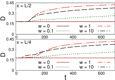
Figure 3: The time evolution of the particle density $D(x,t)$ arising from the protocol outlined in Sec. II.3, in the presence of pumping/decay boundary dissipative mechanisms, for $\bar{\mu}_{i}=\bar{\mu}=0$, $L=360$, $x=L/4$ (bottom) and $x=L/2$ (top), and various values of $w$, versus the time $t$. Note that it takes some time, $t=t^{*}>0$ to depart from the initial value, corresponding to the time needed for a signal of speed $v_{m}=2$ to travel from the closest end to the site $x$, see text.

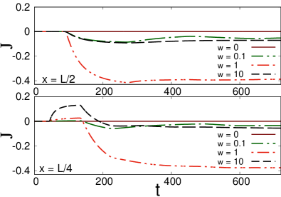
Figure 4: The time evolution of the fermionic current $J(x,t)$, for $\bar{\mu}_{i}=\bar{\mu}=0$, $L=360$, $x=L/4$ (bottom) and $x=L/2$ (top), and various values of $w$, versus the time $t$. In the presence of pumping/decay boundary dissipative mechanisms, the fermionic current becomes nonzero. Of course, the current goes from the end where the bath is pumping particles to the other one where they get lost.

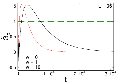
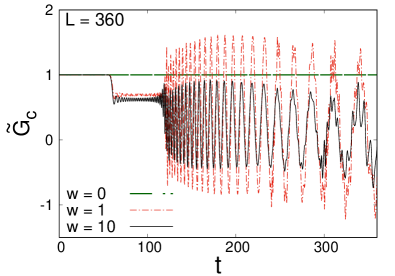
Figure 5: The time volution of the ratio $\widetilde{G}_{c}$, cf. Eq. (18), related to the fixed-time fermionic correlation $G_{c}$, in the presence of pumping/decay boundary dissipative mechanisms, for $\bar{\mu}_{i}=\bar{\mu}=0$, $x=L/3$ and $y=2L/3$ (symmetric with respect to the center of the lattice), and various values of $w$, versus the time $t$. The top figure shows data for $L=36$ up to large times approaching the stationary state. The bottom figure shows data for $L=360$ and relatively small time. In the presence of dissipation $w>0$, we note a significant change of behavior, being characterized by ample oscillations, whose frequency appear approximately independent of $w$, while the oscillation amplitudes are apparently nonmonotonic, being larger for $w=1$ than $w=10$.

Figure 6: Asymptotic large-$t$ values of $J(x,t)$ for $\bar{\mu}=0$ and $x=L/2$ for various sizes $L$. They turn out to be hardly distinguishable. The same results are obtained for any site not involving the ends of the chain. These results provide the dependence on $w$ of the asymptotic large-time limit $f(\bar{\mu},w)$ of the fermionic current $J(x,t)$, cf. Eq. (25), for $\bar{\mu}=0$. Note that $f(0,w)$ is nonmonotonic, indeed its absolute value has a maximum at a finite value $w\approx 1.7265$.

In Figs. 3, 4 and 5, we show some results for the evolution of the particle density, the fermionic current, and the correlation $G_{c}$ respectively, for protocols with pumping and decay dissipative boundaries, when starting from a critical ground state at $\bar{\mu}_{i}=0$. The quantum evolution leads to stationary states depending on $\bar{\mu}$ and $w$, while it is independent of the initial condition, thus independent of $\bar{\mu}_{i}$. The asymptotic stationary state corresponds to the eigenstate of the Lindbladian generator ${\cal L}$ with zero eigenvalue, i.e. it is solution of ${\cal L}(\rho)=0$. The observables defined in Sec. II.3 asymptotically turn out to behave as

$${\rm lim}_{t\to\infty}\;D(x,\bar{\mu}_{i},\bar{\mu},w,t,L)={1/2}\,,$$ (24)

$${\rm lim}_{t\to\infty}\;J(x,\bar{\mu}_{i},\bar{\mu},w,t,L)=f(\bar{\mu},w)\,,$$ (25)

$${\rm lim}_{t\to\infty}\;G_{c/p}(x,y,\bar{\mu}_{i},\bar{\mu},w,t,L)=0\,,$$ (26)

for any sites except those at the ends of the chain that are in contact with the baths (the fermionic density and current take different values at the boundaries). Only the asymptotic large-$t$ fermionic current given by the function $f(\bar{\mu},w)$ shows a behavior dependent on $\bar{\mu}$ and $w$, see Fig. 6, being nonzero and constant for any site $x$ excluded those involving the ends of the chain. The above results can be derived by solving the corresponding dynamic equations, see App. A, in the stationary limit when the time derivatives in the l.h.s. vanish.

The asymptotic stationary states do not appear particularly interesting. However, we are mostly interested in the quantum evolution before approaching the asymptotic stationary states. As we shall see, this turns out to be quite complex, developing two different dynamic regimes: an early-time regime for $t\sim L$, and a large-time regime for $t\sim L^{3}$ that describe the approach to the above stationary states.

We note that in protocols without quenching of the Hamiltonian parameters, thus limiting itself to switch the boundary dissipative interactions on, the observables far from the ends remain unchanged up to a certain time $t=t^{*}>0$, see Figs. 3, 4 and 5 (all obtained without quenching the Hamiltonian parameter $\bar{\mu}$). This fact can be related to the propagation of the quasi-particle modes within the bulk of the system LR-72 ; CC-05 . In the equivalent quantum Ising chain, cf. Eq. (4), their maximum speed is given by $v_{m}=2\,{\rm Min}[g,1]$, CEF-12-1 therefore $v_{m}=2$ at the critical point. For example Fig. 3 shows that the particle density at $x=L/2$ and $x=L/4$ starts departing from its initial value at $t^{*}\approx L/4$ and $t^{*}=L/8$ respectively, which is the time needed for a signal of speed $v_{m}=2$ to arrive at the site $x$, starting from the closest dissipative end at $t=0$. Analogous initial behaviors are observed for the other observables considered.

We also note that the time scale of the signal propagation, i.e. $t\sim L$, is compatible with the time scaling variable $\theta=t/L$ introduced in Sec. III. Therefore, we expect that phenomena related to propagation are essentially encoded in the asymptotic dynamic scaling functions entering Eq. (21). We also mention that the finite-speed propagation of quasi-particle modes gives also rise to peculiar revival phenomena in closed finite-size systems RV-21-rev ; HHH-12 ; KLM-14 ; Cardy-14 ; JJ-17 ; MAC-20 ; RV-21 .

IV.2 The early-time dynamic finite-size scaling

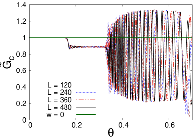
Figure 7: Dynamic scaling of the ratio $\widetilde{G}_{c}(x,y,\bar{\mu}_{i},\bar{\mu},w,t,L)$ associated with the fermionic correlation $G_{c}$, as defined in Eq. (18), for fixed $X=x/L=1/3$, $Y=y/L=2/3$ (so that $Y-X=1/3$), $\kappa_{i}=\kappa=0$, $w=1/4$, versus $\theta=t/L$, for various size $L$ up to $L=480$. These results support the dynamic FSS put forward in Eq. (23), indeed they appear to converge to an asymptotic scaling function of $\theta$, characterized by sizeable oscillations whose amplitude and frequency appear to scale as well. The approach to the asymptotic behavior is globally compatible with the existence of $O(1/L)$ corrections. The case for $w=0$, i.e. no dissipation, is trivially represented by a constant line, $\widetilde{G}_{c}=1$.

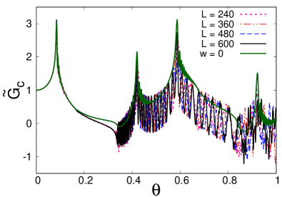
Figure 8: Dynamic scaling of $\widetilde{G}_{c}(x,y,\bar{\mu}_{i},\bar{\mu},w,t,L)$ for fixed $X=x/L=1/3$, $Y=y/L=2/3$ (so that $Y-X=1/3$, top figure) and $X=x/L=3/8$, $Y=y/L=5/8$ (so that $Y-X=1/4$, bottom figure), $\kappa_{i}=0$, $\kappa=3$, $w=1/4$, versus $\theta=t/L$, for various size $L$ up to $L=600$. These results support the dynamic FSS put forward in Eq. (23). The comparison with the case without dissipation, i.e. the $w=0$ curve for $L=480$, show similarities, but very distinct oscillatory behaviors for $w=1/4$.

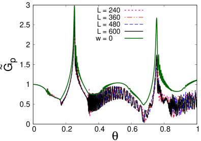
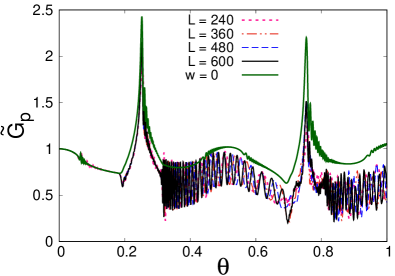
Figure 9: Dynamic scaling of the ratio $\widetilde{G}_{p}(x,y,\bar{\mu}_{i},\bar{\mu},w,t,L)$ associated with the fermionic correlation $G_{p}$, cf. Eq. (18), for fixed $X=x/L=1/3$, $Y=y/L=2/3$ (so that $Y-X=1/3$, top figure) and $X=x/L=3/8$, $Y=y/L=5/8$ (so that $Y-X=1/4$, bottom figure), $\kappa_{i}=0$, $\kappa=3$, $w=1/4$, versus $\theta=t/L$, for various size $L$ up to $L=600$. These results support the dynamic FSS put forward in Eq. (23). For comparison we also report the curve for $w=0$ for $L=480$.

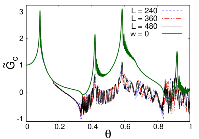
Figure 10: Dynamic scaling of $\widetilde{G}_{c}(x,y,\bar{\mu}_{i},\bar{\mu},w,t,L)$ for a single decay dissipative boundary, for $X=x/L=1/3$ and $Y=y/L=2/3$, at fixed $\kappa_{i}=0$, $\kappa=3$, and $w=10$, versus $\theta=t/L$, for various size $L$ up to $L=480$. Again the dynamic FSS (23) emerges, thus supporting the value $\zeta=0$ for the exponent entering the scaling variable associated with $w$. We again compare with the case in the absence of dissipation, i.e. for $w=0$ (the reported curve is that for $L=480$).

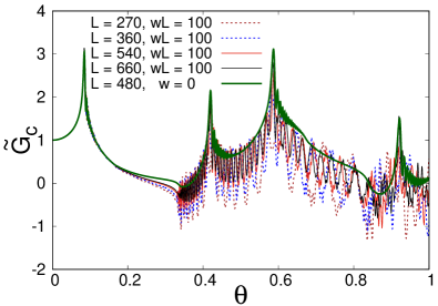
Figure 11: Check of the behavior of the fermionic correlation $\widetilde{G}_{c}(x,y,\bar{\mu}_{i},\bar{\mu},w,t,L)$ when decreasing the dissipation parameter as $w\sim L^{-1}$, like the dynamic scaling for homogenous dissipations. In particolar, we report results for fixed $X=x/L=1/3$, $Y=y/L=2/3$ (so that $Y-X=1/3$), $\kappa_{i}=0$, $\kappa=3$, $wL=100$, versus $\theta=t/L$, for various size $L$ up to $L=660$. The curves appear to approach that in the absence of dissipation, with oscillations whose amplitude is decreasing as $1/L$ approximately.

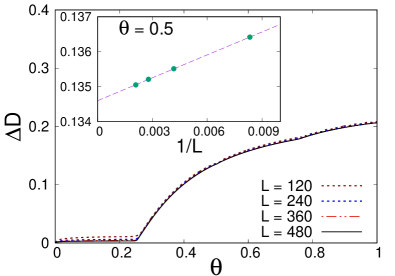
Figure 12: Dynamic scaling of the subtracted particle density $\Delta D(x,\bar{\mu}_{i},\bar{\mu},w,t,L)$ defined in Eq. (27), at fixed $\kappa_{i}=0$, $\kappa=3$, and $w=1$ for various $L$.

We now investigate the early-time regime of the quantum evolution arising from the protocol described in Sec. II.3. This is the regime where $t\sim L$, therefore the appropriate time scaling variable is $\theta=t/L$, like the dynamic FSS developed by closed fermionic Kitaev wires at CQTs, cf. Eq. (15).

To determine the correct scaling associated with the boundary dissipation parameter, and in particular the exponent $\zeta$ in Eq. (23), we compute the time evolution of the fixed-time fermionic correlations $G_{c}$ and $G_{p}$ for various values of $w$. Figs. 7, 8 and 9 show results at fixed $w=1/4$. We show results without quenching the Hamiltonian parameter $\mu$, in Fig. 7, and quenching it around the critical point, in Figs. 8 and 9. Analogous results are observed for other values of $w$. The curves appear to approach an asymptotic scaling behavior matching the FSS ansatz (23), thus supporting the value $\zeta=0$ for the exponent entering the scaling variable associated with $w$. The asymptotic scaling functions appear clearly distinct from those in the absence of dissipation, i.e. for $w=0$. Their comparison shows some similarities, for example the existence of spikes, but very distinct oscillatory behaviors for $w=1/4$, which persist in the dynamic FSS limit. The convergence to the large-$L$ asymptotic behavior is generally consistent with $O(1/L)$ corrections. However, the convergence is expected to be nonuniform, i.e. the amplitudes of the corrections are expected to increase, making it slower and slower with increasing $\theta$, as also shown by the data. Analogous results are also obtained in the case of a single decay dissipative boundary, see Fig. 10 for results with $w=10$.

As a check of the apparent dynamic scaling with $\zeta=0$, in Fig. 11) we show plots obtained by keeping the product $w\,L$ fixed when increasing the size $L$, thus by decreasing the dissipation parameter as $w\sim 1/L$. This is the scaling analogous to the case of homogenous dissipators, cf. Eqs. (20) and (21). In this case, the curves appear to approach the scaling function of the close system for $w=0$, and the oscillations gets suppressed as $1/L$.

Therefore, we conclude that the dynamic FSS developed by the fermionic correlations $G_{c/p}$ within the early-time regime is compatible with a vanishing exponent $\zeta$ in Eq. (23), and exclude the value $\zeta=1$. Of course our numerical analysis cannot really distinguish $\zeta=0$ from a small value, say $|\zeta|\lesssim 0.2$. A more conclusive evidence for $\zeta=0$ would require exact computations in the dynamic FSS limit, or numerical results for much larger chains. A simple (likely naive) interpretation of the evidence in favor of $\zeta=0$ may be related to the fact that the dynamic FSS for homogenous bulk dissipation requires $w\sim L^{-z}$, but it involves a number $L$ of dissipators as in Fig. 2. On the other hand, the boundary dissipation arises from a number of dissipators smaller by a $O(1/L)$ factor. Therefore, one might interpret the vanishing of $\zeta$ as the result of the simple relation $\zeta=z-1=0$. We believe that this point deserve further investigation, for example by checking it in other models, with CQTs characterized by different critical exponents.

We also show some results for the particle density, in particular for the difference

$$\Delta D(x,t)=D(x,t)-D(x,t=0)\,,$$ (27)

see Fig. 12. They show an apparent scaling behavior when plotted versus $\theta$, demonstrating that the early-time scale of the variations of the particle density is $t\sim L$ as well. However, this scaling behavior does not come from the original critical modes, since their contributions are suppressed as $O(L^{-y_{n}})$, thus as $O(L^{-1})$, see Eq. (14). Analogous results are obtained for the fermionic current.

We finally note that the asymptotic dynamic scaling behaviors of the correlations, reported in Figs. 7-11, are characterized by the presence of cusps, thus indicating a nonanalytic time dependence in the rescaled time variable $\theta$. This features are reminiscent of the behavior at the so-called dynamical phase transitions HPK-13 ; Heyl-18 . Likely, they deserve further investigation.

IV.3 Large-time regime approaching stationary states

The approach to the asymptotic stationary states are generally controlled by the Liouvillian gap $\Delta_{\cal L}$ associated with the generator ${\cal L}$, cf. Eq. (1). BP-book ; RH-book ; Znidaric-15 ; MBBC-18 ; SK-20 . The asymptotic stationary state is provided by the eigenstate of ${\cal L}$ with vanishing eigenvalue, $\Lambda_{0}=0$, while all other eigenstates have eigenvalues $\Lambda_{i}$ with negative real part, i.e. ${\rm Re}\,\Lambda_{i}<0$ for any $i>0$. The approach to the stationary state is controlled by Liouvillian gap $\Delta_{\cal L}$ which is given by the eigenvalue with the largest nonzero real part, i.e.

$$\Delta_{\cal L}=-{\rm Max}_{i>0}\,{\rm Re}\,(\Lambda_{i})\,.$$ (28)

As shown in Ref. RV-19, , in the case of homogenous dissipative schemes (like that in Fig. 2), the conjectured dynamic scaling, such as that in Eq. (21), describes also the approach to the asymptotic stationary states. Indeed, for homogenous local dissipative mechanisms such as pumping or decay, $\Delta_{\cal L}$ scales as $\Delta_{\cal L}\sim 1/L$ when keeping $\gamma=uL$ fixed, analogously to the critical gap $\Delta_{L}\sim 1/L$ at the CQT of the Kitaev wire. Therefore, the dynamic scaling can follow the whole dynamic process from $t=0$ to the asymptotic stationary states. This is supported by the data in Fig. 13, which show that the dynamic FSS ansatz (21) describes the whole quantum dynamics from $t=0$ to the corresponding asymptotic stationary states. Note that Fig. 13 reports results for fermionic wires with open boundary conditions, thus extending the evidence of dynamic FSS already reported in Refs. NRV-19, ; RV-19, for systems with antiperiodic boundary conditions.

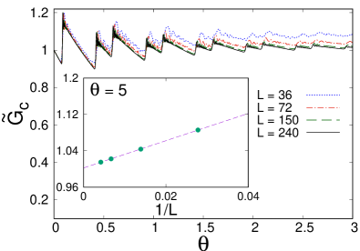
Figure 13: Evolution of $\widetilde{G}_{c}(x,y,\bar{\mu}_{i},\bar{\mu},u,t,L)$ for the homogenous decay dissipation mechanisms, such as those sketched in Fig. 2, and for $X=x/L=1/3$ and $Y=y/L=2/3$, for $\bar{\mu}_{i}=\bar{\mu}=0$, and $\gamma=uL=1$ fixed, versus $\theta=t/L$, for various size $L$ up to $L=240$. The inset shows the $1/L$ convergence at $\theta=5$.

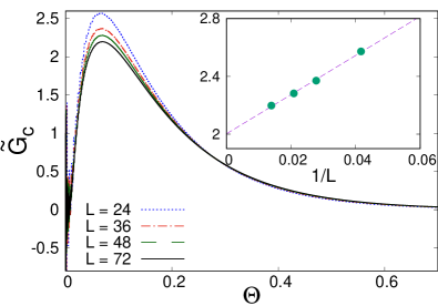
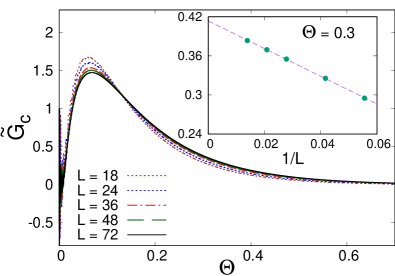
Figure 14: Evolution of $\widetilde{G}_{c}(x,y,\bar{\mu}_{i},\bar{\mu},w,t,L)$ for the case with pumping/decay boundary dissipations, and for $X=x/L=1/3$ and $Y=y/L=2/3$, for $\kappa_{i}=\kappa=0$ (bottom) and $\kappa_{i}=\kappa=3$ (top), and $w=10$, versus $\Theta=t/L^{3}$, for various size $L$ up to $L=72$. The inset in the top figure shows the large-$L$ convergence at the maximum of the curve, while that of the bottom figure shows the convergence at $\Theta=0.3$.

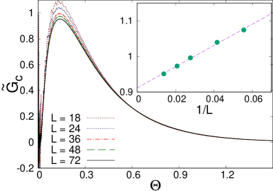
Figure 15: Evolution of $\widetilde{G}_{c}(x,y,\bar{\mu}_{i},\bar{\mu},w,t,L)$ with a single decay dissipative boundary, for $X=x/L=1/3$, $Y=y/L=2/3$, $\bar{\mu}_{i}=\bar{\mu}=0$, and $w=10$, versus $\Theta=t/L^{3}$, for various size $L$ up to $L=72$. The inset shows the large-$L$ convergence at the maximum of the curves.

In the case of dissipative boundaries we observe another scenario, for which the approach to the stationary behavior requires a different scaling regime, characterized by much larger times, scaling as $t\sim L^{3}$, instead of $t\sim L$. This is in agreement with analytical and numerical results for quantum spin chains with baths coupled at the ends of chain PP-08 ; Prosen-08 ; Znidaric-15 ; SK-20 , where the Liouvillian gap behaves as $\Delta_{\cal L}\sim L^{-3}$. Indeed, we find that in the large-$L$ limit

$$L^{3}\Delta_{\cal L}\approx F(\bar{\mu},w)\,.$$ (29)

In particular the function $F(0,w)$ is nonmonotonic with a minimum for $w\approx 1.7265$ in correspondence of the maximum of the absolute value of the fermionic current, see Fig. 6. These results imply that the asymptotic approach to stationarity in Kitaev wires with dissipative pumping/decay boundary dissipation is associated with a large time regime scaling as $t\sim L^{3}$.

In Figs. 14 and 15 we show some results for the fermionic correlation in the case of boundary dissipations at both ends and at only one end, respectively. They definitely support the asymptotic dynamic scaling in the terms of the scaling time variable

$$\Theta=tL^{-3}\,.$$ (30)

This regime is again controlled by the interplay between the Hamiltonian parameter $\bar{\mu}$ and the dissipative rate $w$. The results hint at the dynamic scaling behavior

$$\widetilde{G}_{c/p}(x,y,\bar{\mu}_{i},\bar{\mu},w,t,L)\approx\widetilde{G}_{c/p}(X,Y,\kappa_{i},\kappa,\Theta,w)\,.$$ (31)

Note that within this large-time regime the system looses the memory of the initial the critical condition of the system, approaching a noncritical stationary state.

V Conclusions

We have investigated how the presence of boundary dissipative interactions (see Fig. 1) affects the quantum critical dynamics of many-body systems at CQTs, i.e. when the Hamiltonian parameters driving the unitary dynamics get tuned to their critical values, leading to a vanishing gap and a diverging length scale.

As a paradigmatic model, we consider the quantum fermionic Kitaev wires, defined by the Hamiltonian (3), and subject to dissipative interactions at the boundaries, associated with particle pumping and decay mechanisms. They are induced by couplings with a Markovian bath, such that the evolution of the system density matrix can be effectively described by a Lindblad master equation, such as Eq. (1). The Kitaev wire with pumping/decay dissipative interactions is particularly convenient for numerical computations, indeed it allows us to perform numerical computations for relatively large systems, and therefore to achieve accurate checks of the dynamic scaling behaviors in the presence of dissipative interactions with the environment, see also Refs. NRV-19, ; RV-19, ; RV-20, ; DRV-20, . In our study we address the relevance of dissipative boundaries at CQTs, i.e. whether they maintain the system within a critical regime, or they make the system depart from criticality. Moreover, we check if their effects can be casted within a dynamic scaling framework as in the case of homogenous dissipative mechanisms.

To address the quantum dynamic resulting from the competition of the unitary Hamiltonian and boundary dissipative drivings, we consider protocols (see Sec. II.3) based on an instantaneous quenching of the Hamiltonian parameters and turning on of the dissipative interactions, starting at $t=0$ from ground states of the Hamiltonian with parameters close to their critical values. Analogous protocols were also considered to address the effects of homogenous dissipative interactions involving the bulk of the system NRV-19 ; RV-19 ; RV-20 ; DRV-20 , as sketched in Fig. 2, so that we can make an interesting comparison of the effects of bulk and boundary dissipations described within the analogous Lindblad framework.

On the one hand, in the case of bulk homogenous dissipation at quantum transitions, the quantum dynamics of systems of size $L$ can be described within dynamic FSS frameworks where the relevant scaling variable associated with time is $\theta=tL^{-z}\sim t\Delta_{L}$ (where $\Delta_{L}\sim L^{-z}$ is the vanishing gap of the critical Hamiltonian), and the global dissipative rate $u$ must be tuned to zero as $u\sim\Delta_{L}\sim L^{-z}$ with $z=1$. The out-of-equilibrium dissipative quantum dynamics shows essentially one dynamic regime, from the beginning to the large-time asymptotic behavior.

On the other hand, quantum fermionic wires with boundary dissipations show notable differences. In particular their quantum evolution during the above mentioned protocol show two different dynamic regimes. There is an early-time regime for times $t\sim L$, where the competition between coherent and incoherent drivings develops a dynamic FSS analogous to that applying to bulk dissipations, but the boundary dissipative-rate parameter $w$ does not require to be tuned to zero. Then there is a large-time regime for $t\sim L^{3}$ whose dynamic scaling describes the late quantum evolution leading to the $t\to\infty$ stationary states. The large time scales $t\sim L^{3}$ are essentially related to the slowest decay of the Lindbladian gap $\Delta_{\cal L}\sim L^{-3}$, which characterize several quantum spin chains and fermionic wires with boundary dissipations PP-08 ; Prosen-08 ; Znidaric-15 ; SK-20 .

We present various numerical results for systems with decay and pumping dissipative interactions with equal dissipation rate at their ends, and also dissipative interactions localized to one end only. The emerging scaling scenarios appear similar, thus we believe that their validity extends to more general situations with localized dissipative interactions. For example one may consider periodic wires close to quantum transitions with one, or more then one, localized dissipative interactions with external sources.

Further investigations are called for, to achieve a deeper understanding of the effects of boundary dissipative interactions at quantum transitions. In this respect, a crucial role is played by the exponent $\zeta$ entering the scaling law (23), and controlling the scaling of the boundary dissipation parameters. Our numerical results show that it is compatible with zero in fermionic Kitaev wires with pumping and decay boundary dissipative mechanisms. An interesting question is whether it assumes different values in other one-dimensional models with boundary dissipations, which may be also related to mechanisms that are not describable by Lindblad equations, such as baths with an infinite set of harmonic oscillators CL-83 ; Leggett-etal-87 . Other interesting issues concern higher-dimensional systems with dissipative interactions around the boundaries. Moreover, one may also address the effects of boundary dissipations at first-order quantum transitions, which are characterised by an extreme sensitivity to the boundary properties CPV-14 ; PRV-18 ; PRV-20 ; DRV-20 .

Appendix A Some details on the numerical computations

To compute the time evolution of an observable $A(t)$ associated with an operator $\hat{A}$,

$$A(t)={\rm Tr}[\rho(t)\,\hat{A}]\,,$$ (32)

such as those defined in Sec. II.3, we solve corresponding coupled differential equations, formally obtained from the Lindblad master equation (1), as

$${\partial\over\partial t}A(t)={\rm Tr}[{\cal L}(\rho)\,\hat{A}]\,,\qquad A(0)={\rm Tr}[\rho_{i}\,\hat{A}]\,.$$ (33)

To the purpose of computing the observables introduced in Sec. II.3, we consider the quantities

$$\mathscr{C}_{x,y}(t)={\rm Tr}[\rho(t)\,\hat{c}_{x}^{\dagger}\hat{c}_{y}^{\phantom{\dagger}}]\,,\quad\mathscr{P}_{x,y}(t)={\rm Tr}[\rho(t)\,\hat{c}_{x}^{\dagger}\hat{c}_{y}^{\dagger}]\,.\quad$$ (34)

Then, straightforward computations allow us to derive the linear equations

$$\frac{d}{dt}\,\mathscr{C}_{x,y}=i\,(\mathscr{C}_{x,y+1}-\mathscr{C}_{x-1,y}+\mathscr{C}_{x,y-1}-\mathscr{C}_{x+1,y})\qquad$$ (35)

$$\quad-i\,(\mathscr{P}_{y,x-1}^{\dagger}-\mathscr{P}_{y,x+1}^{\dagger}-\mathscr{P}_{x,y-1}+\mathscr{P}_{x,y+1})$$

$$\quad-\frac{w}{2}\,(\delta_{L,y}\,\mathscr{C}_{x,L}+\delta_{L,x}\,\mathscr{C}_{L,y}+\delta_{1,y}\,\mathscr{C}_{x,1}+\delta_{1,x}\,\mathscr{C}_{1,y})$$

$$\quad+w\,\delta_{L,y}\,\delta_{L,x}\,,$$

$$\frac{d}{dt}\,\mathscr{P}_{x,y}=-i\,(\mathscr{P}_{x,y+1}+\mathscr{P}_{x+1,y}+\mathscr{P}_{x,y-1}+\mathscr{P}_{x-1,y})$$

$$\quad-i\,(\mathscr{C}_{x,y-1}-\mathscr{C}_{y,x-1}-\mathscr{C}_{x,y+1}+\mathscr{C}_{y,x+1})$$

$$\quad-i\,(\delta_{x-1,y}-\delta_{x+1,y})-2\,i\,\mu\,\mathscr{P}_{x,y}$$

$$\quad-\frac{w}{2}\,(\delta_{1,y}\,\mathscr{P}_{x,1}+\delta_{1,x}\,\mathscr{P}_{1,y}+\delta_{L,y}\,\mathscr{P}_{x,L}+\delta_{L,x}\,\mathscr{P}_{L,y})\,.$$

These coupled equations must be solved using the initial conditions $\mathscr{C}_{x,y}(0)={\rm Tr}[\rho_{i}\,\hat{c}_{x}^{\dagger}\hat{c}_{y}^{\phantom{\dagger}}]$ and $\mathscr{P}_{x,y}(0)={\rm Tr}[\rho_{i}\,\hat{c}_{x}^{\dagger}\hat{c}_{y}^{\dagger}]$, where $\rho_{i}$ is the initial pure-state density matrix corresponding to the ground state of the Hamiltonian for $\bar{\mu}_{i}$. They can be computed using standard diagonalization techniques, see, e.g., Ref. Blaizot-book, . Then differential equations are solved using the four-order Runge-Kutta method. Finally, the observables defined in Sec. II.3 are easily obtained by $D(x,t)=\mathscr{C}_{x,x}(t)$, $J(x,t)=-2\,{\rm Im}\,\mathscr{C}_{x+1,x}(t)$, $G_{c}(x,y,t)=2\,{\rm Re}\,\mathscr{C}_{x,y}(t)$, and $G_{p}(x,y,t)=2\,{\rm Re}\,\mathscr{P}_{x,y}(t)$.

We finally describe how we obtained the asymptotic stationary behaviors reported in Eqs. (24), (25), and (26). First, we solved Eqs. (35) in the stationary limit for systems of finite size $L$ using exact diagonalization, by assuming that the time derivatives in the l.h.s. vanish. The results turn out to rapidly converge to their large-$L$ limit, as for example shown by the data reported in Fig. 6. This allows us to obtain a robust guess of their large-$L$ limits, such as those reported in Eqs. (24), (25), and (26). Then we verified that they exactly solve the coupled equations in the stationary and large-$L$ limits. Of course, these results are consistent with the asymptotic large-time convergence of the observables in the time evolution arising from the dynamic protocol.

References

- (1) A. A. Houck, H. E. Türeci, and J. Koch, On-chip quantum simulation with superconducting circuits, Nat. Phys. 8, 292 (2012).
- (2) M. Müller, S. Diehl, G. Pupillo, and P. Zoller, Engineered open systems and quantum simulations with atoms and ions, Adv. At. Mol. Opt. Phys. 61, 1 (2012).
- (3) I. Carusotto and C. Ciuti, Quantum fluids of light, Rev. Mod. Phys. 85, 299 (2013).
- (4) M. Aspelmeyer, T. J. Kippenberg, and F. Marquardt, Cavity optomechanics, Rev. Mod. Phys. 86, 1391 (2014).
- (5) M. J. Hartmann, Quantum simulation with interacting photons, J. Opt. 18, 104005 (2016).
- (6) C. Noh and D. G. Angelakis, Quantum simulations and many-body physics with light, Rep. Prog. Phys. 80, 016401 (2017).
- (7) F. Minganti, A. Biella, N. Bartolo, and C. Ciuti, Spectral theory of Liouvillians for dissipative quantum transitions, Phys. Rev. A 98, 042118 (2018).
- (8) Y. Li, X. Chen, and M. P. A. Fisher, Measurement-driven entanglement transition in hybrid quantum circuits, Phys. Rev. B 100, 134306 (2019).
- (9) B. Skinner, J. Ruhman, and A. Nahum, Measurement-induced phase transitions in the dynamics of entanglement, Phys. Rev. X 9, 031009 (2019).
- (10) D. Rossini and E. Vicari, Coherent and dissipative dynamics at quantum phase transitions, arXiv:2103.02626, submitted to Physics Reports.
- (11) S. Yin, P. Mai, and F. Zhong, Nonequilibrium quantum criticality in open systems: The dissipation rate as an additional indispensable scaling variable, Phys. Rev. B 89, 094108 (2014).
- (12) S. Yin, C.-Y. Lo, and P. Chen, Scaling behavior of quantum critical relaxation dynamics of a system in a heat bath, Phys. Rev. B 93, 184301 (2016).
- (13) D. Nigro, D. Rossini, and E. Vicari, Competing coherent and dissipative dynamics close to quantum criticality, Phys. Rev. A 100, 052108 (2019).
- (14) D. Rossini and E. Vicari, Scaling behavior of stationary states arising from dissipation at continuous quantum transitions, Phys. Rev. B 100, 174303 (2019).
- (15) D. Rossini and E. Vicari, Dynamic Kibble-Zurek scaling framework for open dissipative many-body systems crossing quantum transitions, Phys. Rev. Research 2, 023211 (2020).
- (16) S. L. Sondhi, S. M. Girvin, J. P. Carini, and D. Shahar, Continuous quantum phase transitions, Rev. Mod. Phys. 69, 315 (1997).
- (17) S. Sachdev, Quantum Phase Transitions, (Cambridge University, Cambridge, England, 1999).
- (18) G. Di Meglio, D. Rossini, and E. Vicari, Dissipative dynamics at first-order quantum transitions, Phys. Rev. B 102, 224302 (2020).
- (19) M. Campostrini, J. Nespolo, A. Pelissetto, and E. Vicari, Finite-size scaling at first-order quantum transitions, Phys. Rev. Lett. 113, 070402 (2014).
- (20) H.-P. Breuer and F. Petruccione, The Theory of Open Quantum Systems (Oxford University Press, New York, 2002).
- (21) A. Rivas and S. F. Huelga, Open Quantum System: An Introduction (SpringerBriefs in Physics, Springer, 2012).
- (22) G. Lindblad, On the generators of quantum dynamical semigroups, Commun. Math. Phys. 48, 119 (1976).
- (23) V. Gorini, A. Kossakowski, and E. C. G. Sudarshan, Completely positive dynamical semigroups of N-level systems, J. Math. Phys. 17, 821 (1976).
- (24) L. M. Sieberer, M. Buchhold, and S. Diehl, Keldysh field theory for driven open quantum systems, Rep. Prog. Phys. 79, 096001 (2016).
- (25) A. D’Abbruzzo and D. Rossini, Self-consistent microscopic derivation of Markovian master equations for open quadratic quantum systems, Phys. Rev. A 103, 052209 (2021).
- (26) A. Yu. Kitaev, Unpaired Majorana fermions in quantum wires, Phys. Usp. 44, 131 (2001).
- (27) T. Prosen and I. Pizorn, Quantum Phase Transition in a Far-from-Equilibrium Steady State of an XY Spin Chain, Phys. Rev. Lett. 101, 105701 (2008).
- (28) T. Prosen, Third quantization: a general method to solve master equations for quadratic open Fermi systems, New J. Phys. 10, 043026 (2008).
- (29) L. Bianchi, P, Giorda, and P. Zanardi, Quantum information-geometry of dissipative quantum phase transitions, Phys. Rev. E 89, 022102 (2014).
- (30) M. Znidaric, Relaxation times of dissipative many-body quantum systems, Phys. Rev. E 92, 042143 (2015).
- (31) L. M. Vasiloiu, F. Carollo, and J. P. Garrahan, Enhancing correlation times for edge spins through dissipation, Phys. Rev. B 98, 094308 (2018).
- (32) H. Fröml, A. Ciocchetta, C. Kollath, and S. Diehl, Fluctuation-Induced Quantum Zeno Effect, Phys. Rev. Lett. 122, 040402 (2019)
- (33) F. Tonielli, R. Fazio, S. Diehl, and J. Marino, Orthogonality catastrophe in dissipative quantum many body systems, Phys. Rev. Lett. 122, 040604 (2019).
- (34) W. Berdanier, J. Marino, and E. Altman, Universal Dynamics of Stochastically Driven Quantum Impurities, Phys. Rev. Lett. 123, 230604 (2019).
- (35) P. L. Krapivsky, K. Mallick and D. Sels, Free fermions with a localized source, J. Stat. Mech. (2019) 113108.
- (36) N. Shibata and H. Katsura, Quantum Ising chain with boundary dephasing, Prog. Theor. Exp. Phys. 12A108 (2020).
- (37) S. Wolff, A. Sheikhan, S. Diehl, and C. Kollath, Non-equilibrium metastable state in a chain of interacting spinless fermions with localized loss, Phys. Rev. B 101, 075139 (2020).
- (38) H. Fröml, C. Muckel, C. Kollath, A. Ciocchetta, and S. Diehl, Ultracold quantum wires with localized losses: many-body quantum Zeno effect, Phys. Rev. B 101, 144301 (2020)
- (39) D. Rossini, A. Ghermaoui, M. Bosch Aguilera, R. Vatrè, R. Bouganne, J. Beugnon, F. Gerbier, and L. Mazza, Strong correlations in lossy one-dimensional quantum gases: from the quantum Zeno effect to the generalized Gibbs ensemble, Phys. Rev. A 103, L060201 (2021).
- (40) V. Alba and F. Carollo, Noninteracting fermionic systems with localized dissipation: Exact results in the hydrodynamic limit, arXiv:2103.05671.
- (41) B. Horstmann and J. I. Cirac, Noise-driven dynamics and phase transitions in fermionic systems, Phys.Rev. A 87, 012108 (2013).
- (42) M. Keck, S. Montangero, G. E. Santoro, R. Fazio, and D. Rossini, Dissipation in adiabatic quantum computers: lessons from an exactly solvable model, New. J. Phys. 19, 113029 (2017).
- (43) D. Nigro, On the uniqueness of the steady-state solution of the Lindblad-Gorini-Kossakowski-Sudarshan equation, J. Stat. Mech. (2019) 043202.
- (44) W. H. Zurek and U. Dorner and P. Zoller, Dynamics of a quantum phase transition, Phys. Rev. Lett. 95, 105701 (2005).
- (45) A. Polkovnikov, Universal adiabatic dynamics in the vicinity of a quantum critical point, Phys. Rev. B 72, 161201 (2005).
- (46) J. Dziarmaga, Dynamics of a quantum phase transition: Exact solution of the quantum Ising model, Phys. Rev. Lett. 95, 245701 (2005).
- (47) S. Deng, G. Ortiz, and L. Viola, Dynamical non-ergodic scaling in continuous finite-order quantum phase transitions, Eur. Phys. Lett. 84, 67008 (2009).
- (48) C. De Grandi, V. Gritsev, and A. Polkovnikov, Quench dynamics near a quantum critical point, Phys. Rev. B 81,012303 (2010).
- (49) S. Gong, F. Zhong, X. Huang, and S. Fan, Finite-time scaling via linear driving, New J. Phys. 12, 043036 (2010).
- (50) A. Chandran, A. Erez, S. S. Gubser, S. L. Sondhi, Kibble-Zurek problem: Universality and the scaling limit, Phys. Rev. B 86, 064304 (2012).
- (51) M. Kolodrubetz, B. K. Clark, and D. A. Huse, Nonequilibrium dynamic critical scaling of the quantum Ising chain, Phys. Rev. Lett. 109, 015701 (2012).
- (52) A. Francuz, J. Dziarmaga, B. Gardas, and W. H. Zurek, Space and time renormalization in phase transition dynamics, Phys. Rev. B 93, 075134 (2016).
- (53) A. Pelissetto, D. Rossini, and E. Vicari, Dynamic finite-size scaling after a quench at quantum transitions, Phys. Rev. E 97, 052148 (2018).
- (54) A. Pelissetto, D. Rossini, and E. Vicari, Out-of-equilibrium dynamics driven by localized time-dependent perturbations at quantum phase transitions, Phys. Rev. B 97, 094414 (2018).
- (55) E. Vicari, Decoherence dynamics of qubits coupled to systems at quantum transitions, Phys. Rev. A 98, 052127 (2018).
- (56) D. Rossini and E. Vicari, Scaling of decoherence and energy flow in interacting quantum spin systems, Phys. Rev. A 99, 052113 (2019).
- (57) D. Nigro, D. Rossini, and E. Vicari, Scaling properties of work fluctuations after quenches near quantum transitions, J. Stat. Mech. (2019) 023104.
- (58) M. Campostrini, A. Pelissetto, and E. Vicari, Finite-size scaling at quantum transitions, Phys. Rev. B 89, 094516 (2014).
- (59) P. Calabrese, M. Caselle, A. Celi, A. Pelissetto, and E. Vicari, Nonanalyticity of the Callan-Symanzik -function of two-dimensional O() models, J. Phys. A 33, 8155 (2000).
- (60) M. Caselle, M. Hasenbusch, A. Pelissetto, and E. Vicari, Irrelevant operators in the two-dimensional Ising model, J. Phys. A 35, 4861 (2002).
- (61) P. Pfeuty, The one-dimensional Ising model with a transverse field, Ann. Phys. 57, 79 (1970).
- (62) E. H. Lieb and D. W. Robinson, The finite group velocity of quantum spin systems, Commun. Math. Phys. 28, 251 (1972).
- (63) P. Calabrese and J. Cardy, Evolution of Entanglement Entropy in One-Dimensional Systems, J. Stat. Mech. (2005) P04010.
- (64) P. Calabrese, F. H. Essler, and M. Fagotti, Quantum quench in the transverse field Ising chain: I. Time evolution of order parameter correlators, J. Stat. Mech. (2012) P07016.
- (65) J. Häppölä, G. B. Halász and A. Hamma, Universality and robustness of revivals in the transverse field XY model, Phys. Rev. A 85, 032114 (2012).
- (66) P. L. Krapivsky, J. M. Luck and K. Mallick, Survival of classical and quantum particles in the presence of traps, J. Stat. Phys. 154, 1430 (2014)
- (67) J. Cardy, Thermalization and revivals after a quantum quench in conformal field theory, Phys. Rev. Lett. 112, 220401, (2014).
- (68) R. Jafari and H. Johannesson, Loschmidt echo revivals: Critical and noncritical, Phys. Rev. Lett. 118, 015701 (2017).
- (69) , R. Modak, V. Alba and P. Calabrese, Entanglement revivals as a probe of scrambling in finite quantum systems, J. Stat. Mech. (2020) 083110.
- (70) D. Rossini and E. Vicari, Dynamics after quenches in one-dimensional quantum Ising-like systems, Phys. Rev. B 102, 054444 (2020); Phys. Rev. B 103, 179901(E) (2021).
- (71) M. Heyl, A. Polkovnikov, and S. Kehrein, Dynamical Quantum Phase Transitions in the Transverse-Field Ising Model, Phys. Rev. Lett. 110, 135704 (2013).
- (72) M. Heyl, Dynamical quantum phase transitions: a review, Rep. Prog. Phys. 81, 054001 (2018).
- (73) A. O. Caldeira and A. J. Leggett, Quantum tunnelling in a dissipative system, Ann. Phys. 149, 374 (1983).
- (74) A. J. Leggett and S. Chakravarty and A. T. Dorsey and M. P. A. Fisher and A. Garg and W. Zwerger, Dynamics of the dissipative two-state system, Rev. Mod. Phys. 59, 1 (1987).
- (75) A. Pelissetto, D. Rossini, and E. Vicari, Scaling properties of the dynamics at first-order quantum transitions when boundary conditions favor one of the two phases, Phys. Rev. E 102, 012143 (2020).
- (76) J.-P. Blaizot and G. Ripka, Quantum Theory of Finite Systems, MIT Press, 1986.