latexOverwriting file
Consensus Based Sampling
Abstract
We propose a novel method for sampling and optimization tasks based on a stochastic interacting particle system. We explain how this method can be used for the following two goals: (i) generating approximate samples from a given target distribution; (ii) optimizing a given objective function. The approach is derivative-free and affine invariant, and is therefore well-suited for solving inverse problems defined by complex forward models: (i) allows generation of samples from the Bayesian posterior and (ii) allows determination of the maximum a posteriori estimator. We investigate the properties of the proposed family of methods in terms of various parameter choices, both analytically and by means of numerical simulations. The analysis and numerical simulation establish that the method has potential for general purpose optimization tasks over Euclidean space; contraction properties of the algorithm are established under suitable conditions, and computational experiments demonstrate wide basins of attraction for various specific problems. The analysis and experiments also demonstrate the potential for the sampling methodology in regimes in which the target distribution is unimodal and close to Gaussian; indeed we prove that the method recovers a Laplace approximation to the measure in certain parametric regimes and provide numerical evidence that this Laplace approximation attracts a large set of initial conditions in a number of examples.
Keywords.- stochastic interacting particle systems, sampling, optimization
1 Introduction
1.1 Background
We consider the inverse problem of finding from where
| (1.1) |
Here is the observation, is the unknown parameter, is the forward model and is the observational noise. We adopt the Bayesian approach to inversion [42] and assume that the parameter and the noise are independent and normally distributed: and . By (1.1) and Bayes’ formula, the posterior density (i.e., the conditional probability density function of given ) equals
| (1.2) |
where
| (1.3) |
In the foregoing and in what follows, we adopt the following notation: for a positive definite matrix ,
We also define the matrix norm (noting that this is not the induced matrix norm from vector norm ).
Solving inverse problems in the Bayesian framework can be prohibitively expensive because of the need to characterize an entire probability distribution. One approach to this is simply to seek the point of maximum posterior probability, the MAP point [42, 20], defined by
| (1.4) |
However, this essentially reduces the solution of the inverse problem to a classical optimization approach [25] and fails to capture uncertainty. A compromise between a fully Bayesian approach and the classical optimization approach is to seek a Gaussian approximation of the measure [50]. By the Bernstein–von Mises theorem (and its extensions) [70], the posterior is expected to be well approximated by a Gaussian density in the large data limit, if the parameter is identifiable in the infinite data setting; a Gaussian approximation is also expected to be good if the forward map is close to linear. For these reasons, use of the Laplace method [66] to obtain a Gaussian approximation of the posterior density is often viewed as a useful approach in many application domains.
Many inverse problems arising in applications are defined by complex forward models , often available only as a black box, and in particular adjoints and derivatives may not be readily available. Consensus-based approaches are proving to be interesting and viable derivative-free techniques for optimization [60, 11, 15]. The focus of this paper is on developing consensus-based sampling of the posterior distribution for Bayesian inverse problems and, in particular, on the study of such methods in the context of Gaussian approximation of the posterior.
The computational methodology we introduce applies to arbitary measures with negative log density , and is not restricted to the choice in (1.3) resulting from the inverse problem (1.1). Some of our analysis, however, is specific to the inverse problem in the case where is linear. The proposed methodology is potentially useful for the solution of complex problems for which the evaluation of or is expensive, and derivatives of and are not available, or noisy and not useable. In this sense the proposed methodology is competitive with state-of-the-art ensemble Kalman methods for inverse problems, which are also of particular value for derivative-free sampling when is expensive to evaluate. The fact that the analysis of the accuracy of the proposed sampling method is confined to unimodal distributions which are close to Gaussian is also a limitation of ensemble Kalman methods. Our work thus provides impetus for further innovation in the analysis and design of particle-based, derivative-free sampling methods.
1.2 Literature Review
Systematic procedures to sample probability measures have their roots in statistical physics and the 1953 paper of Metropolis et al [51]. In 1970 Hastings recognized this work as a special case of what is now known as the Metropolis-Hastings methodology [35]. These methods in turn may be seen as part of the broader Markov Chain Monte Carlo (MCMC) approach to sampling [9]. In 2006, sequential Monte Carlo (SMC) methods, based on creating a homotopy deforming the initial (simple to sample) measure into the desired target measure, were introduced [21]; in practice these methods work best when entwined with MCMC kernels. These SMC methods introduce the idea of using the evolution of a system of interacting particles to approximate the desired target measure; the large particle limit of this evolution captures the homotopy from the initial measure to the target measure. In a parallel development, the mathematical physics community has developed a large body of understanding of interacting particle systems, and their mean field limits, initially primarily for models on a countable state space [48, 67] and more recently for models in uncountable state space [68, 13, 4, 5, 40]. Studying interactions between sampling, collective dynamics of particles and mean field limits holds considerable promise as a direction for finding improved sampling algorithms for specific classes of problems and is an active area of research [61, 72, 10, 71].
The focus of this work is on sampling measure (1.2), or optimizing objective function (1.4), by means of algorithms which only involve black box evaluation of . While some MCMC and SMC methods are of this type, the Metropolis algorithm being a primary example, the use of collective dynamics of particles opens the door to a wider range of methods to solve inverse problems in this setting. There are two primary classes of methods emerging in this context: those arising from consensus forming dynamics [60] and those arising from ensemble Kalman methods [62].
Iterative ensemble Kalman methods for inverse problems were introduced in [17, 24]. Similar ideas are also implicit in the work of Reich [61] who studies state estimation sequential data assimilation, rather than the inverse problem; however, what is termed the “analysis” step in sequential data assimilation corresponds to solving a Bayesian inverse problem. These iterative ensemble Kalman methods are similar to SMC in that they seek to map the prior to the posterior in finite continuous time or in a finite number of steps. Reich also introduced continuous time analysis of ensemble Kalman methods for state estimation in [1, 2], naming the resulting algorithm the ensemble Kalman Bucy filter (EnKBF); the ensemble Kalman approach to inverse problems introduced in [17, 24] may be studied using the EnKBF leading to a clear link with SMC methods in continuous time. An alternative Kalman methodology (ensemble Kalman inversion – the EKI) for the optimization approach to the inverse problem, which involves iteration to infinity, was introduced and studied in [38, 37] in discrete time and in [64, 65] in continuous time; the idea of using ensemble methods for optimization rather than sampling was anticipated in [61]. The ensemble based optimization approach was generalized to approximate sampling of the Bayesian posterior solution to the inverse problem in [30] (the ensemble Kalman sampler – the EKS), and studied further in [16, 31, 54].
The idea of consensus based optimization may be seen as a variation of particle swarm optimization methods [22, 44] which are themselves related to Cucker-Smale dynamics for collective behavior and opinion formation [69, 19, 34, 4, 13, 53]. These dynamical systems model the tendency of the constituent particles to align (consensus in velocity) or to concentrate in certain variables modelling averaged quantities (consensus in position or opinion), and they have been extensively studied in terms of long time asymptotics leading to consensus [12, 53]. Consensus Based Optimization (CBO) was introduced in [60] based on the following simple idea: particles are explorers in the landscape of the graph of the function to be minimized, they are able to exchange information instantaneously, and they redirect their movement towards the location of a consensus position in parameter space that is a weighted average of the explorer’s parameter values relative to the Gibbs measure associated to the function , . Noise is introduced for suitable exploration in parameter space but the strength of the noise is reduced according to the distance to the consensus parameter values. These effects lead to concentration in parameter space at the global minimum of the function, as proven in [11] for the mean-field limit PDE and in [33] for the particle system under certain conditions on and the parameters of the model. The original CBO method has been recently improved so as to be efficient for high-dimensional optimization problems [15], such as those arising in machine learning, by adding coordinate-wise noise terms and introducing ideas from random batch methods [41] for computing stochastic particle systems efficiently. Furthermore, these ideas have been recently used to solve constraint problems on the sphere [27, 28, 29]. There are other approaches to the use of interacting particles system in optimization, including the use of individual gradient dynamics coupled through a graph Laplacian [8, 6, 7, 43].
The development of the EKI into the EKS suggests a parallel development of CBO into a sampling methodology. In this paper we pursue this idea and develop Consensus Based Sampling (CBS). A key property of the EKS is that it is affine invariant [32] as shown in the paper [31] where the Affine Invariant Interacting Langevin Dynamics (ALDI) algorithm is introduced; relatedly, in the mean field limit, the rate of convergence to the posterior is the same for all Gaussian posterior distributions [30]. We will show identical properties for the CBS algorithm. Our focus is on unimodal distributions and obtaining Gaussian approximations to the target distribution. We note, however, that there are recent forays into the use of ensemble Kalman methods for the sampling of multimodal distributions [63, 49]. Furthermore there is also recent work extending ensemble Kalman methods to inverse problems beyond the setting of additive Gaussian noise; more complex loss functions, such as cross-entropy and those arising in logistic regression [45, 59] are considered. And finally, recent work shows that ensemble methods automatically smooth noisy likelihood functions, essentially denoising rough energy landscapes [23]. Similar developments for the CBS methodology proposed here would also be of interest. Like the ensemble Kalman sampler, the CBS approach is only exact for Gaussian problems and in the mean field limit. However recently developed methods based on multiscale stochastic dynamics provide a refineable methodology for sampling from non-Gaussian distributions [57]; methods such as CBS or EKS may be used to precondition these multiscale stochastic dynamics algorithms, making them more efficient. Alternatively, the CBS method may be used in the calibration step employed within the calibrate-emulate-sample methodology introduced in [18]. Thus, the methods developed in this paper potentially form an important component in an efficient and rigorously justifiable approach to solving Bayesian inverse problems.
1.3 Our Contributions
We introduce CBS as a method to approximate probability distributions of the form (1.2), or to find the MAP estimator (1.4). The method requires only as a black-box (it is derivative-free) and hence is of potential use for large-scale inverse problems. We study the proposed algorithm in settings where the posterior is Gaussian or close to Gaussian. We reemphasize that the computational methodology does not require the specific choice of in (1.3), it applies to arbitary measures with negative log density , up to an additive constant; however some of our analysis exploits the specific form in (1.3) in the case where is linear. We show the following:
-
•
in the case of linear , and in the mean field limit, parameters can be chosen in the algorithm so that, if initiated at a Gaussian, successive iterates remain Gaussian and converge to the Gaussian posterior (1.2);
-
•
in the case of linear , and in the mean field limit, parameters can be chosen in the algorithm so that, if initiated at a Gaussian, successive iterates remain Gaussian and converge to a Dirac located at the MAP point given by (1.4);
-
•
the CBS method is affine invariant and, in the case of linear and in the mean field limit, converges at the same rate across all linear inverse problems defined by (1.2); for linear , we obtain sharp convergence rates that are explicit in terms of all parameters of the method;
-
•
in the case of nonlinear , and in the mean field limit, parameters can be chosen in the algorithm so that it has a steady state solution which is Gaussian, close to the Laplace approximation of the posterior (1.2) and the algorithm is a local contraction mapping in the neighbourhood of the steady state; we make explicit the dependence of this approximation, and its rate of attraction, on the parameters of the method;
-
•
we present numerical results illustrating the foregoing theory and, more generally, demonstrating the viability of the CBS scheme for sampling posterior distributions and for finding MAP estimators.
The results are in arbitrary dimension , with the exception of the results concerning the Laplace approximation which are restricted to . There are no intrinsic barriers to extending the Laplace approximation results to arbitrary dimension, but doing so will be technically involved and would lose the focus of the paper.
In Section 2 we introduce the method, including its continuous time limit, and mean field limits in both discrete and continuous time; we establish its properties in the Gaussian setting. Section 3 contains analysis of the method beyond the Gaussian setting, deriving conditions for convergence to an approximation of the MAP estimator when in optimization mode, and for convergence to the Laplace approximation of the target measure when in sampling mode. In Section 4 we provide the numerical experiments. Proofs of most of the theoretical results in Sections 2 and 3 are presented in Section 5.
2 Presentation of the Method
We propose a novel method for sampling and optimization tasks based on a system of interacting particles. Our goals are the following:
- (1)
-
(2)
Optimization: to find the minimizer of , which corresponds to the MAP point (1.4), the most likely parameter given the data and the model relating them.
In order to introduce the approach, we start by defining the mean-field limits of the algorithms, in discrete and continuous time; later we explain how particle approximations of the mean-field limit lead to implementable algorithms. We will be interested in the following McKean difference equation: given parameters , and ,
| (2.1) |
where , for are independent random variables, and denote respectively the mean and variance for a suitable reweighting of measures:
| (2.2a) | |||
| (2.2b) | |||
Letting and viewing as a discrete time approximation of a continuous time process at time , we find that the continuous-time limit associated with these dynamics is the following McKean SDE:
| (2.3) |
where denotes a standard Brownian motions in d. We refer to the two familes of methods as Consensus Based Sampling (CBS) methods, parameterized by with the ranges corresponding to (2.1) and corresponding to (2.3). Recall that . We will focus on two choices of : (i) the choice , when the method is used to minimize , which will be referred to as CBS-O(,); and (ii) when the method is used for sampling the target distribution , which will be referred to as CBS(,).
In Subsection 2.1, we introduce the notation used throughout the paper. In Subsection 2.2 we give motivation for the mean field stochastic dynamical systems (2.1) and (2.3). In Subsection 2.3 we describe key properties of the mean field models, and in Subsection 2.4, we establish convergence to equilibrium for (2.1) and (2.3) in the setting where the forward model is linear and the law of the initial condition is Gaussian. Subsection 2.5 introduces particle approximations to the mean field limit.
2.1 Notation
In what follows, we denote by the density of the Gaussian random variable :
| (2.4) |
We also use the short-hand notation
| (2.5) |
More generally, we frequently denote and for the standard mean and covariance calculated with respect to a probability measure . For a matrix , we denote by the operator norm induced by the Euclidean vector norm, and by the Frobenius norm111The Frobenius norm on matrices should not to be confused with the norm on vectors defined previously. . Sometimes, we will make use of the shorthand notation for a given invertible matrix . We let and , and we denote by the set of symmetric strictly positive definite matrices in d×d. For symmetric matrices and , the notation (resp. ) means that is positive semidefinite (resp. negative semidefinite).
2.2 Motivation
The mean-field model (2.1) contains a number of tuneable parameters. In this section we give intuition about the role of these parameters in effecting approximate sampling or optimization for the inverse problem defined by (1.1). We motivate sampling primarily through the discrete time mean field model and optimization primarily through the continuous time mean field model. However both discrete and continuous time models apply to optimization and to sampling. In practice, the mean field SDEs in this subsection can be made into algorithms by invoking finite particle approximations, as described in Subsection 2.5.
2.2.1 Sampling.
Let be a linear map so that the posterior distribution given by (1.2) is Gaussian, and denote this Gaussian by . The mean and covariance may be identified by completing the square in (1.2): is of the form ,
To motivate the algorithms that are the object of study in this paper we describe parameter choices for which the iteration (2.1) has equilibrium distribution given by the Gaussian . For any choice of forward model , it can be shown that the evolution of the first and second moments is given by
| (2.6a) | ||||
| (2.6b) | ||||
From these identities it is clear that any fixed point of the mean and covariance is independent of Further, when the initial distribution is Gaussian the systems of equations (2.1) for map Gaussians into Gaussians. Computing the relationship between the mean and covariance of the Gaussian and the mean and covariance of the Gaussian gives
| (2.7a) | ||||
| (2.7b) | ||||
Therefore, the mean and covariance of a non-degenerate Gaussian steady state for (2.1) satisfes
This has solution
Choosing delivers a steady state equal to the posterior distribution. This motivates our choice of in the sampling case. Furthermore, choosing is seen to be natural in the optimization setting: the fixed point of the iteration is then a Dirac at the MAP estimator We will demonstrate that these two distinguished choices of work well for sampling and optimization, beyond the setting of a Gaussian posterior .
Remark 2.1 (Enlarging the Choice of Parameters.).
The mean-field dynamics (2.1) can be generalized to the form
| (2.8) |
where are independent random variables. Given , one can ask the following question: for what values of the parameters does the dynamics (2.8) admit the Gaussian as an equilibrium distribution? A calculation analogous to that above shows that is a steady state of (2.8) if and only if
| (2.9a) | |||
| (2.9b) | |||
Note that these constraints do not guarantee that is the only steady state, and in fact, if and , then any distribution is a steady state. In this paper, we study only the dynamics (2.1), which corresponds to the special case where and , and , but it is potentially useful to exploit this wider class of mean-field models.
2.2.2 Optimization.
We now discuss the algorithm in optimization mode, through the lens of the continuous time limit. Another starting point triggering the research in this paper is the use of systems of interacting particles for minimizing a target function . The papers [60, 11] introduce the CBO technique for achieving this aim by means of particle appoximations of the stochastic dynamical system
| (2.10) |
where is a standard Brownian motion in d, is the noise strength and is the law of The idea behind the CBO method is to think about realizations of as explorers, in the landscape of the function , which can continuously exchange the evaluation of the function at their position , through Then, the explorers compute a weighted average of their position in parameter space and direct their relaxation movement towards this average ; this explains the first term on the right hand side of (2.10). The role of the second term is to impose the property of noise strength decreasing proportionally to the distance of the explorer to the weighted average . The choice of the weighted average promotes the concentration towards parameter points leading to smaller values of . The resulting law of the system converges as towards a Dirac mass concentrated at the MAP point , the global minimizer of , under certain conditions on ; see [11, 33]. The weighted covariance provides an alternative to the cooling schedule in (2.10) by way of using as the modulation of the noise. In other words, one could propose as alternative to the CBO method (2.10), the following mean field system
| (2.11) |
This gives (2.3) in the optimization mode . We show in Proposition 2.6 for the quadratic case, and Proposition 3.8 for the one-dimensional convex case, that (2.11) converges precisely to the minimizer of , whereas the CBO method usually concentrates to a point in the vicinity of the minimizer, with an error depending on . On the other hand, while the CBO dynamics concentrates exponentially fast under rather general assumptions on , including the multidimensional non-convex setting [11, 15], the dynamics (2.11) converges algebraically in time and our proofs concern only simple settings, considering quadratic or one-dimensional convex functions . Adapting the parameter during the evolution is shown empirically to improve the rate of convergence for (2.11), see the discussions in Section 4; but analysis is needed to understand this property. Other differences between the methods are that, unlike CBO, the dynamics (2.11) is affine invariant (see Subsection 2.3.2) and satisfies the invariant subspace property (see Lemma 2.7), although further investigation is necessary to determine whether these two properties are useful in the context of optimization.
In terms of time complexity, one iteration of (the particle approximations of) either method requires the evaluation of at all the particles; thus, in the context of Bayesian inverse problems where evaluating the forward model is the dominating computational expense, the methods have a similar computational cost per iteration. For problems where the dimension of the state space is very large and evaluation of is cheap, however, the particle method corresponding to (2.11) is slightly more expensive than that of (2.10), as it requires calculating the square root of large matrices . We note, however, that employing a generalized square root as proposed in [31] for the ALDI method would help to mitigate this difficulty.
2.3 Key Properties of the Mean Field Limits
In this subsection, we summarize key properties of the stochastic dynamics (2.1) and (2.3). We consider, in turn: (i) the time evolution of the laws; (ii) the affine invariance; (iii) the steady states; (iv) the evolution of the first and second moments; and (v) propagation properties for Gaussian initial conditions.
2.3.1 Evolution Equations for the Law of the Mean Field Dynamical Systems.
The time evolution of the law of the solution (2.1) is governed by the following discrete-time dynamics on probability densities:
| (2.12) |
When , the map (2.12) takes a particularly simple form (recalling notation 2.4 for a Gaussian):
| (2.13) |
Likewise, the time evolution of the law of the solution to (2.3) is governed by the following nonlinear and nonlocal Fokker–Planck equation:
| (2.14) |
Remark 2.2.
We will not discuss here the question of existence and uniqueness of solutions to (2.14), and we assume from now on that there exists a unique strong solution to (2.14) for smooth initial data , implying in turn the existence and uniqueness of a solution to (2.3). The equation (2.14) will be analyzed in subsequent work.
2.3.2 Affine Invariance.
A fundamental property of both (2.1) and (2.3) is that they are affine invariant, in the sense of [32]; the utility of this concept has been established for MCMC methods in [46] and for Langevin based dynamics through the ALDI algorithm in [31]. For linear inverse problems with posterior this has the consequence that the rate of convergence is independent of the conditioning of . We study affine invariance of (2.1); a similar reasoning can be employed to show that the continuous-time mean-field dynamics (2.3) are also affine invariant.
In order to demonstrate affine invariance for (2.1), let denote the solution to (2.1) with initial condition , and let . Consider a vector and an invertible matrix which, together, define the affine transformation . We introduce the following notation:
We also introduce and . To prove the affine invariance of the scheme (2.1), we must show that is equal in law to the solution of
| (2.15) |
with initial condition and where are independent random variables. In order to show this, we apply the affine transformation to both sides of (2.1), which leads to
Now notice that , where , that
and that , which implies that is indeed a solution to (2.15).
2.3.3 Steady States.
The steady states of (2.1) and (2.3) coincide, if they exist, and they are necessarily Gaussian. Recall the notation (2.4). We have:
Lemma 2.1.
Let probability distribution have finite second moment and be a steady-state solution of (2.12) or (2.14). Then
| (2.16) |
Conversely, all probability distributions solving (2.16) are steady states of (2.12) and (2.14). In particular, all steady states are Gaussian (with the limiting case of Diracs included in the definition) and all Dirac masses are steady states.
2.3.4 Equations for the Moments.
The evolution equations for the moments given in (2.6) hold regardless of whether is Gaussian but they define closed equations characterizing completely in settings where is Gaussian. The evolution of the moments can also be written for the limiting continuous time stochastic dynamical system (2.3) obtained when :
| (2.18a) | ||||
| (2.18b) | ||||
2.3.5 Propagation of Gaussians.
We show that Gaussianity is preserved along the flow, both in discrete and continuous time.
Lemma 2.2.
Let and .
Proof.
For the discrete-time dynamics in setting (i), this follows directly from (2.13). For (ii) note that, if , then , being the sum of Gaussian random variables as given in (2.1), is also normally distributed.
In order to show (iii), we consider a solution to the moment equations (2.20). Then solves (2.14). To see this, one can verify that general Gaussians satisfy the relations
for any ; see similar computations in [30, 16]. The first identity can be checked directly, and the second identity follows e.g. from equations (57) and (61) in [58]. Then
where we used the explicit expression of in the last equation. ∎
2.4 Convergence for Gaussian Targets
In this subsection, we consider the case of a linear forward map in (1.1), leading to the posterior distribution being a Gaussian where, throughout, we assume that is strictly positive definite, . The corresponding potential is given by the quadratic function . Recall the shorthand notation . Throughout this section, we denote
The main convergence results of this subsection, Propositions 2.4, 2.5 and 2.6, establish the convergence of the moments of the solutions to (2.1) and (2.3), respectively, in the case of Gaussian initial conditions. All results show algebraic convergence in optimization mode () and exponential convergence in sampling mode (); this is analogous to what is known about the EKI [64] and the EKS [30] methods. We provide in Table 1 an overview of the results we obtain. Most proofs of the results presented in the rest of this subsection are given in Subsection 5.1.
| Sampling | Optimization | |||
|---|---|---|---|---|
| Mean | Covariance | Mean | Covariance | |
We draw a number of conclusions from these results. Firstly, in the discrete time setting, smaller choices of provide a faster rate of convergence, and choosing is therefore the most favorable choice in this regard. Secondly, larger choices of increase the speed of convergence, without limit as for ; in the case , increasing is favourable but does not give rates which increase without limit.
2.4.1 Convergence Analysis for the Discrete-Time Dynamics.
Using the explicit expression of the weighted moments in the Gaussian case (2.7), we can rewrite the right-hand sides of 2.19 as
Letting and , we can verify that solves the following recurrence relation:
| (2.21a) | ||||
| (2.21b) | ||||
This is a recurrence relation uniquely solvable given initial conditions . We begin by studying the easier case , where the convergence of the scheme can be computed explicitly by a direct argument.
Lemma 2.3.
Consider the iterative scheme (2.13) with and initial conditions . Then, for any and , we have
Proof.
When , the evolution equations (2.21) for the moments simplify to
For , the result for the covariance matrix is easily obtained by solving the second equation explicitly for . Next, consider the case . We have
For the evolution of the mean, notice that
Hence, and the result follows. ∎
We deduce from this result a convergence estimate for the mean and the covariance of the iterates.
Proposition 2.4.
Consider the iterative scheme (2.13) with and initial conditions . Then the following statements hold:
-
(i)
Sampling mode . For all , it holds that
-
(ii)
Optimization mode . For all , it holds that
In order to study the convergence in the general case , we will reduce the evolution of the moments (2.21) to the scalar case,
| (2.22a) | ||||
| (2.22b) | ||||
by diagonalization. Then, using Lemma A.1, the asymptotic behavior of the moments can be summarized as follows.
Proposition 2.5.
Consider the iterative scheme (2.1) with and initial conditions . Then the following statements hold:
-
(i)
Sampling mode . For all ,
-
(ii)
Optimization mode . For all , it holds that
2.4.2 Convergence Analysis for the Continuous-time Dynamics.
Next, we consider the limiting case . Rewriting the right-hand side of (2.20a) and (2.20b) using (2.7), we obtain for any and ,
| (2.23a) | ||||
| (2.23b) | ||||
Proposition 2.6.
Let denote the solution to 2.23 with initial conditions . Then the following statements hold:
-
(i)
Sampling mode . For all ,
-
(ii)
Optimization mode . For all , it holds
Remark 2.3 (Discrete to Continuum).
Notice that, by letting in the convergence results obtained for in Proposition 2.5 and taking the limit , we recover the convergence results of the continuous-time setting, up to the constant prefactor.
Remark 2.4 (Sharpness).
It is possible to show, using the lower bounds on the trend to equilibrium provided by Lemmas A.1 and A.2, that the convergence rates we obtained in Propositions 2.5 and 2.6 are all sharp with respect to and respectively. Note that the argument leading to Proposition 2.5 also applies to the case . However, the upper bounds we obtain in Proposition 2.4 are stronger than those we would be able to obtain by applying Lemma A.1 for . Lower bounds for the sampling mode in the case can be obtained the same way as for . In optimization mode (, we can derive lower bounds explicitly using the expression from Lemma 2.3 as follows: for , we have , so
The conclusion from the above observations is that all rates provided in Table 1 are sharp.
Remark 2.5 (Attractor).
As a consequence of the above convergence results for linear objective functions , the steady state is the unique attractor of the moment equations (2.19) and (2.20) when taking an initial condition with . Therefore, whilst the mean-field dynamics (2.12) and (2.14) admit infinitely many steady states given by all Dirac distributions in addition to the Gaussian steady state , the solutions to the mean-field dynamics always converge to the desired target measure when initialized at Gaussian initial conditions with , avoiding the manifold of Diracs along the evolution.
2.5 Particle Approximations
In this subsection we describe particle approximations of the mean field dynamics (2.1) and (2.3). This leads to the implementable algorithms used in Section 4. The following is a discrete-time system of interacting particles in d with mean field limit given by (2.1):
| (2.26) |
Here , for and , are independent random variables, and is the empirical measure associated with the particle system at iteration ,
We note that
| (2.27a) | ||||
| (2.27b) | ||||
The limit cases and for fixed and reduce to simpler systems. Indeed, in the case where , the method simplifies to
On the other hand, when , the particle evolution 2.26 may be viewed as a time discretization with timestep of the following continuous-time interacting particle system, in which we generalize the notation (2.27) to continuous time in the obvious way:
| (2.28) |
where are independent standard Brownian motions in d. The formal mean field limit of this equation is given by (2.3).
We note that the finite-dimensional particle systems (2.26) and (2.28) are both affine invariant; the proof is similar to that given for the mean-field limit. In addition, like ensemble Kalman based methods for inverse problems [39], the particle systems (2.26) and (2.28) both satisfy the following invariant subspace property.
Lemma 2.7.
Let denote the linear span of . Then for all and for all .
Proof.
We prove only the first claim, which follows from a simple recursion. Let us assume the claim is true for and prove that it is then also true for . Let , where is the orthogonal complement of in d. Taking the inner product of both sides of (2.26) with , we obtain for all that
and so by the Cauchy–Schwarz inequality,
because by the formula (2.27b) for the weighted covariance . Since was arbitrary in , the proof is complete. ∎
Remark 2.6 (Cooling schedule).
To improve algorithmic implementations it will be of value to develop a rigorous understanding of the relationship between the number of particles and the parameter needed to establish good performance of the method. Relatedly, it will also be useful to investigate theoretically the rate of convergence to equilibrium in the setting where a cooling schedule is employed for . See Section 4 for numerical investigations in this direction.
3 Analysis Beyond The Gaussian Setting
In this section, we study the proposed method (2.1) in the case where the function is not necessarily quadratic, and so the target probability distribution may be non-Gaussian. We begin, in Subsection 3.1, by presenting preliminary bounds on and defined in (2.5), and then we analyze the optimization () and sampling () methods in Subsections 3.2 and 3.3, respectively. The proofs of all results are presented in Section 5, with the exception of Theorem 3.9 which is presented in-text.
The results in this section are based on the following two assumptions.
Assumption 1 (Convexity of the potential).
The function satisfies and for all , for some and some .
Assumption 1 guarantees the existence of a unique global minimizer for , which we will denote throughout this section by
Assumption 2 (Bound from above on the Hessian).
The function satisfies and for all , for some and some .
These assumptions are very similar to the ones made in [11] in order to show the convergence of the CBO method [60] for global optimization. The convergence results we present in this section are summarized in Table 2.
| Sampling | Optimization | |||
|---|---|---|---|---|
| Mean () | Covariance () | Mean () | Covariance (any ) | |
3.1 Preliminary Bounds
We first obtain sharp bounds on which, in the special case when is quadratic, enable to recover (2.7b). The first bound relies on a logarithmic Sobolev inequality for the probability measure , where is the normalization constant.
Lemma 3.1 (Upper bound on weighted covariance).
If Assumption 1 holds, then
Remark 3.1.
We note that, by the standard Holley–Stroock result, see e.g. [47, Theorem 2.11], a similar bound could be obtained when is of the type , where satisfies the convexity property Assumption 1 and is a bounded function.
The next lemma provides a bound from below on .
Lemma 3.2 (Lower bound on weighted covariance).
If Assumption 2 holds, then
We now obtain a crude bound on the weighted first moment , which will be our starting point for establishing the existence of a steady state for the sampling scheme. This bound is useful because it shows that for any fixed and .
Lemma 3.3 (Bound on weighted mean).
If Assumptions 1 and 2 hold, then there exists a positive constant such that,
Unfortunately, this bound degenerates in the limit . In spatial dimension one, we will obtain, in the proof of Proposition 3.7, a finer bound on the weighted mean that can be used for proving convergence of the optimization scheme.
3.2 Analysis of the Optimization Scheme
In this subsection, we are concerned with the large-time convergence of the law of the solutions to the mean-field evolution equations (2.1) and (2.3) when and under the following assumption on the initial condition:
Assumption 3 (Non-degenerate Gaussian initial conditions).
Under this assumption, following Lemma 2.2, the solutions are normally distributed for all (discrete or continuous) times with the first and second moments evolving according to 2.19 and (2.20), respectively. We will show that, under appropriate assumptions, the mean converges to and the covariance to zero.
Throughout this subsection, we denote by a solution to (2.19) with , and by a solution to (2.20) with . We also denote by and solutions to (2.12) and (2.14), respectively.
We begin by showing that the covariance matrices decrease to zero with rates matching those obtained in the case of quadratic in Subsection 2.4, up to constant prefactors.
Proposition 3.4 (Collapse of the ensemble in optimization mode).
Let and and assume that Assumption 1 holds. Then we have
-
(i)
Discrete time . If , then
(3.1) -
(ii)
Discrete time . If , then
(3.2) -
(iii)
Continuous time . If , then
(3.3)
Ideally, we would like to show that and ; however, we were able to show this result only in the one-dimensional setting. In the multi-dimensional case, we establish the following weaker result.
Theorem 3.5.
Let , , , and suppose that Assumptions 1 and 2 hold. If there exists such that for some or for , then is the minimizer of .
It follows from the identity
| (3.4) |
where denotes the quadratic Wasserstein distance, that Proposition 3.4 and Theorem 3.5 can be combined in order to obtain convergence results for the solutions to the mean field systems (2.12) and (2.14). For example, the following result holds in the discrete-time case.
Corollary 3.6.
Suppose that Assumptions 1, 2 and 3 hold. If there exists such that , then .
In the one-dimensional case, it is possible to prove the convergence of and to the minimizer without the a priori assumption that and have a limit.
Proposition 3.7 (Convergence in the one-dimensional case).
Let , , , , and suppose that Assumptions 1 and 2 are satisfied. Then it holds that for and, likewise, for .
As above, this result can be combined with Proposition 3.4 to obtain a convergence result in Euclidean Wasserstein distance for the solution to (2.12) and (2.14), under Assumptions 1, 2 and 3. When deriving this convergence result, we obtain non-optimal rates of order for the case , for and for , with .
To conclude this section, we present a convergence result for with an explicit sharp rate in the particular case .
Proposition 3.8 (Rate of convergence).
Let , , , , and suppose that Assumptions 1 and 2 are satisfied. Suppose additionally that is, together with all its derivatives, bounded from above uniformly in . Then there exists a positive constant such that, for sufficiently large ,
The rate of convergence obtained in Proposition 3.8 is almost optimal in view of the fact shown in Subsection 2.4 that scales with as in the case when is quadratic. We expect the result to extend to other values of and to the continuous-time solution to (2.20), but we focus on the case in order to avoid overly lengthy and technical proofs. We point out that, already in the Gaussian case, the argument to obtain an optimal decay rate for is quite technical. Finding a simplified argument to prove optimal rates in the optimization setting is an interesting open problem, which we leave for future work.
3.3 Analysis of the Sampling Scheme
In this subsection, we investigate the existence of steady states and convergence for the mean field dynamics associated with the consensus-based samplers, that is when used with . We consider both the iteration (2.12) (in the case ) and the nonlocal, nonlinear Fokker–Planck equation (2.14) (in the case ).
We begin by stating an existence result in the multi-dimensional setting. Since the corresponding proof is very short, we include it in this section.
Theorem 3.9 (Existence of steady states).
Let , and . Suppose Assumptions 1 and 2 are satisfied. Then there exists such that, for all , the dynamics (2.12) and (2.14) admit a Gaussian steady state satisfying
Proof.
By Lemma 2.1, a Gaussian is a steady state if and only if
i.e. if and only if is a fixed point of the map
In order to prove the result, we show that for all sufficiently large, where
and , with the constant from Lemma 3.3. Since is continuous, the result then follows from Brouwer’s fixed point theorem. By Lemmas 3.1 and 3.2, it holds that for any , so we have to show only that there exist such that
If , then by Lemma 3.3 there exists such that
from where the statement follows easily with . ∎
This result shows that the sampling scheme admits a steady state whose mean is close to the minimizer of for large , but it does not provide much information on the covariance of the Gaussian steady state. In the one-dimensional setting, we can show that the steady state is in fact unique and arbitrarily close to the Laplace approximation of the target distribution provided that is sufficiently large. By the Laplace approximation of the target distribution, we mean the Gaussian probability distribution , that is
(Note that coincides with the target distribution when is quadratic.) In order to establish results in the one-dimensional setting, we make the following additional assumption on .
Assumption 4.
Let . The function is smooth and, together with all its derivatives, it is bounded from above by the reciprocal of a Gaussian, in the sense that for all there exists such that
We let and denote by the closed ball of radius around .
Theorem 3.10 (Convergence to the steady state).
Let and , and suppose Assumptions 1 and 4 hold. For any , there exists and such that the following statements hold for all :
- •
-
•
Discrete time . If Assumption 3 holds and the moments of the initial (Gaussian) law satisfy , then the solution to the iterative scheme 2.12 converges geometrically to the steady state provided that . More precisely,
-
•
Continuous time . If Assumption 3 holds and the moments of the initial (Gaussian) law satisfy , then the solution to the mean field Fokker Planck equation (2.14) converges exponentially to the steady state provided that . More precisely,
There is no conceptual obstruction to generalizing this result to the multi-dimensional setting, but the associated calculations involving the Laplace’s method, on which the proof of Theorem 3.10 relies, are significantly more technical than in the one-dimensional setting, so we focus here on the one-dimensional case only.
4 Numerical Experiments
In this section, we present numerical experiments illustrating our method. The performance of CBS in optimization mode is studied in Subsection 4.1. We then illustrate the efficacy of the method for sampling in Subsection 4.2, where a simple inverse problem with low-dimensional parameter and data is considered, and in Subsection 4.3, where a more realistic and challenging example is examined. Video animations associated with the numerical experiments presented in this section are freely available online [14].
4.1 General-Purpose Optimization
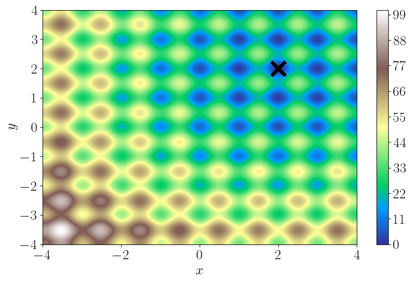
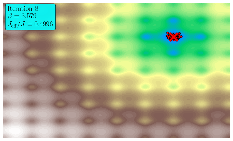
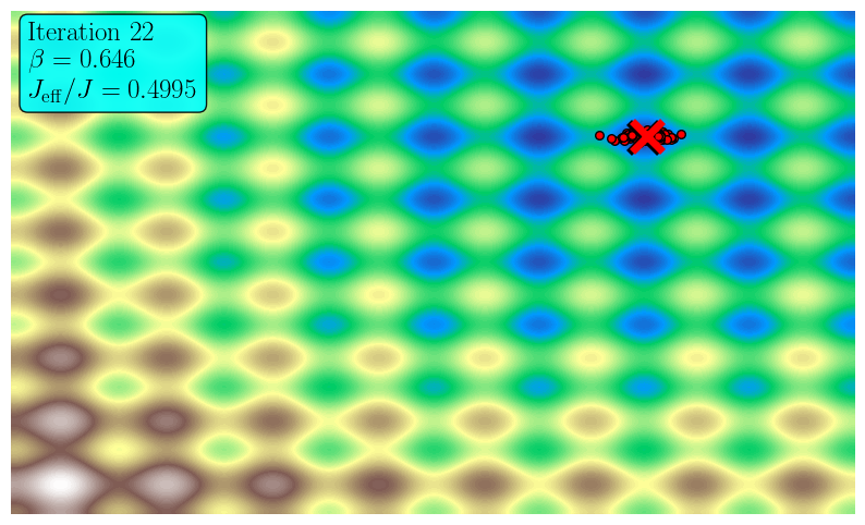
In this subsection, we study the efficacy of our method for solving optimization problems that do not necessarily originate from a Bayesian context. We also show empirically how the convergence of the algorithm can be improved by adapting the parameter appropriately during the simulation. Throughout the subsection, we consider the same non-convex test functions as those taken in [60]: the translated Ackley function, defined for by
| (4.1) |
and the Rastrigin function, defined by
| (4.2) |
Both functions are minimized at , where is a translation parameter. They are depicted in Fig. 1.

In all simulations presented below, the initial particle ensemble members are drawn independently from , and the simulation is stopped when for the first time; here denotes the empirical measure associated with the ensemble at iteration .
4.1.1 Dynamic Adaptation of
In this paragraph, we show numerically that adapting dynamically during a simulation can be advantageous for convergence. We consider the following simple adaptation scheme with parameter : denoting by the ensemble at step , the parameter employed for the next iteration is obtained as the positive solution to the following equation:
| (4.3) |
Employing the notation , we calculate
so is a continuous, non-increasing function with and . Consequently, equation (4.3) admits a unique solution in . The left-hand side of (4.3) is known in statistics as an effective sample size, which motivates the notation . When this approach is employed, the parameter is generally small in the early stage of the simulation as long as the initial ensemble has large enough spread, and it increases progressively as the simulation advances and the ensemble spread decreases. In other words, this cooling schedule for ensures that roughly always the same proportion of particles contribute to the weighted sums in the scheme. This adaptation approach is useful for a two primary reasons:
-
•
On the one hand, provided that and are sufficiently large, adapting according to (4.3) ensures that situations where the ensemble quickly collapses to a very narrow distribution do not arise. An early collapse of the ensemble is not desirable as the scheme may then get stuck in local minima of the objective function , or in the case when the collapse is not complete, the convergence is slowed down considerably. This issue is especially critical when the scheme (2.26) is employed with : in this case, if is not sufficiently small at the beginning of the simulation, it is often the case that the weighted covariance of the initial ensemble is very close to zero, in which case the ensemble collapses nearly to a point in a single step.
-
•
On the other hand, increasing in the later stage of the simulation significantly accelerates convergence to the minimizer. Indeed, when a fixed value of is employed, the weights all converge to the same value as the simulation progresses and the ensemble collapses, and so the influence of the objective function on the dynamics diminishes. By increasing dynamically, we strengthen the bias of the dynamics towards areas of small , thereby accelerating convergence.
In the remainder of this section, we consider for simplicity only the choice . A more detailed analysis of the efficiency of this approach, through both theoretical and numerical means, is left for future work. More generally, an interesting open question is whether it is possible to determine an optimal cooling schedule for taking the above considerations into account. We illustrate in Table 3 the performance of CBS in optimization mode, with both fixed and adaptive , for finding the minimizer of the Ackley function with in dimension 2. The data presented in each cell are calculated from 100 independent runs of the method. For all the values of and considered, using the adaptive strategy based on (4.3) provides a significant advantage, in terms of both the number of iterations required for convergence and the accuracy of the approximate minimizer.
| Adapt? | ||||
|---|---|---|---|---|
| no | ||||
| no | ||||
| no | ||||
| yes | ||||
| yes | ||||
| yes |
4.1.2 Low-dimensional Optimization Problem:
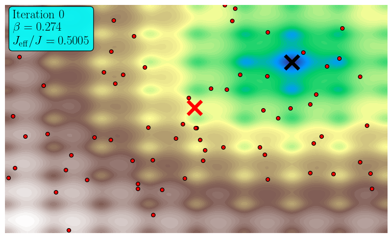
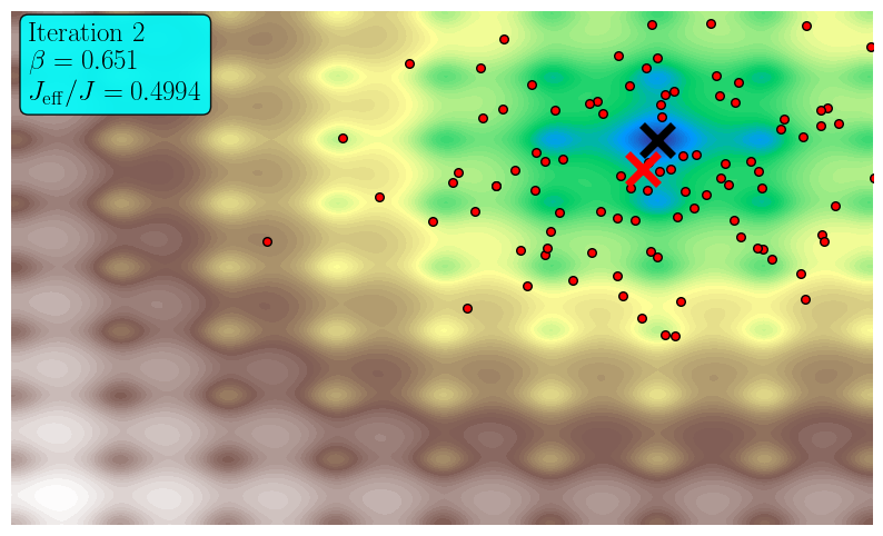
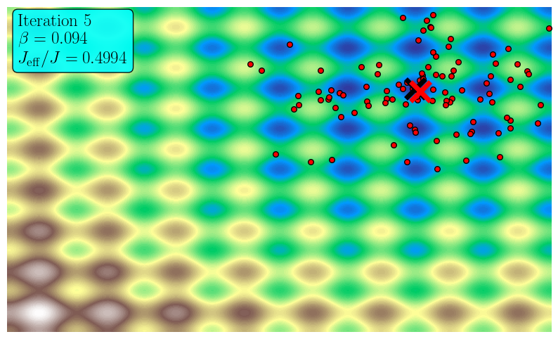
The performance of CBS in optimization mode is illustrated in Tables 4 and 5, for the Ackley and Rastrigin functions respectively, in spatial dimension . We make a few observations:
-
•
Influence of : The simulations corresponding to consistently require fewer iterations to converge than those corresponding to , and they have a better success rate for the Rastrigin function.
-
•
Influence of : For the Rastrigin function, a high number of particles, i.e. a large value of , correlates with a better success rate. With only 50 particles, the method often converges to the wrong local minimizer, but with 200 particles the ensemble almost always collapses at the global minimizer.
-
•
Influence of : For the Rastrigin function, a low value of correlates with better performance. This behavior, which was observed also for CBO in [60], is not surprising because, when , the minimizer is centered with respect to the initial ensemble.
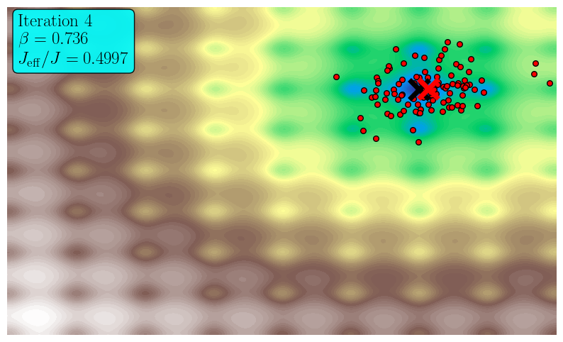
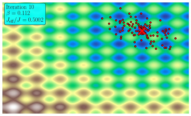
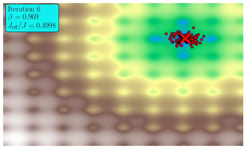
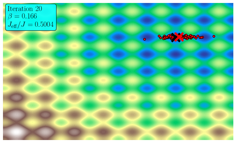
We also note that, like CBO [60], our method performs markedly better for the Ackley function than for the Rastrigin function. Snapshots of the particles are presented in Fig. 2 for the parameters and .

4.1.3 Higher-Dimensional Optimization Problem:
In this paragraph, we repeat the numerical experiments of the previous section in higher dimension . We employ an adaptive in all the simulations, as this approach was shown in the previous subsection to perform much better. The associated results are presented in Tables 6 and 7, which show that the method performs better for small and large for this case as well. Overall, the method seems to require a larger ensemble size than CBO in order to guarantee a similar success rate. A fair comparison of the computational expenses required by both methods is difficult, however, because the number of time steps employed in CBO is not documented in [60].
4.2 Sampling: Low-Dimensional Parameter Space
We first consider an inverse problem with low-dimensional parameter space that was first presented in [26] and later employed as a test problem in [36, 30]. In this problem, the forward model maps the unknown to the observation , where and and where denotes the solution to the boundary value problem
| (4.4) |
with boundary conditions and . This problem admits the following explicit solution [36]:
We employ the same parameters as in [30]: the prior distribution is with , and the noise distribution is with . The observed data is .
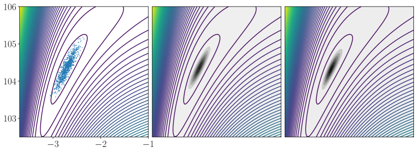
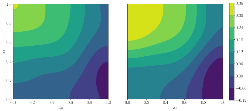
We now investigate the efficiency of (2.26) for sampling from the posterior distribution. To this end, we use the parameters and particles. The ensemble after 100 iterations is depicted in Fig. 3, together with the true posterior. It appears from the figure that the Gaussian approximation of the posterior provided by scheme (2.26) is close to the true posterior, and indeed we can verify that the mean and covariance of the true and approximate posterior distributions, which are given respectively by
and
are fairly close.
4.3 Sampling: Higher-Dimensional Parameter Space
In this section, we consider the more challenging inverse problem of finding the permeability field of a porous medium from noisy pressure measurements in a Darcy flow; for other methods applied to this problem, see [20, 30, 57]. Assuming Dirichlet boundary conditions and scalar permeability for simplicity, we consider the forward model mapping the logarithm of the permeability, denoted by , to the solution of the PDE
| (4.5a) | |||||
| (4.5b) | |||||
Here is the domain and represents a source of fluid. We assume that noisy pointwise measurements of are taken at a finite number equispaced points in , given by
and that these measurements are perturbed by Gaussian noise with distribution , where and . For the prior distribution, we employ a Gaussian measure on with mean zero and precision (inverse covariance) operator given by
equipped with Neumann boundary conditions on the space of mean-zero functions. Here and are parameters controlling the smoothness and characteristic inverse length scale of samples drawn from the prior, respectively. The eigenfunctions and eigenvalues of the covariance operator are
By the Karhunen–Loève (KL) expansion [56], it holds for any that
| (4.6) |
for independent coefficients , and where denotes the -inner product.
In order to approach the problem numerically, we take as object of inference a finite number of terms in the KL expansion of the log-permeability, which may be ordered as a linear vector given an ordering of . The associated prior distribution is given by the finite-dimensional Gaussian , where . At the numerical level, the forward model is evaluated as follows: for a given vector of coefficients , a log-permeability field is calculated by summation as , and the corresponding solution to (4.5) is approximated with a finite element method (FEM). Linear shape functions over a regular mesh with 100 subdivisions per direction are employed for the finite element solution.
For the numerical experiments presented below, a true value for the vector of coefficients is drawn from and employed in order to construct the true permeability field which, in turn, is used with the FEM described above in order to generate the data. In particular, we employ only terms in the KL expansion of the true permeability. We note that, with this approach, the resulting random field should be viewed only as an approximate sample from . Our aim is to study the performance of CBS, not the effect of FEM discretization and truncation of the KL series on the solution of the inverse problem.
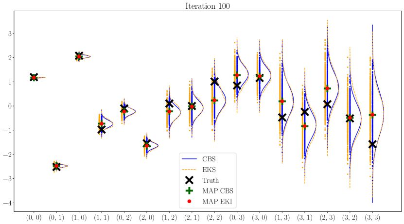
The ensemble obtained after 100 iterations of CBS with adaptive , with and with is depicted in Fig. 4, along with the marginals of the Gaussian distribution with the same first and second moments as the empirical measure associated with the ensemble. The particles forming the initial ensembles were drawn independently from . In order to validate our results, we use as point of reference the solution provided by the ensemble Kalman sampling method [30], combined with the adaptive time-stepping scheme from [45]. It appears from the simulations that the agreement between the posterior distribution obtained by CBS and that obtained by ensemble Kalman sampling is very good, and both approximate posteriors are in good agreement with the true solution.
Using the final ensemble as initial condition for (2.26) in optimization mode, and running 50 more iterations of the algorithm, one obtains an approximation of the MAP estimator, whose associated permeability field is illustrated in Fig. 5. Here we use as point of comparison the solution provided by the ensemble Kalman inversion approach [38]. We present below the values of the first 9 Karhunen–Loève coefficients of (i) the true permeability, (ii) the MAP estimator obtained by CBS, and (iii) the MAP estimator obtained by ensemble Kalman inversion:
(All the numbers displayed here were rounded to two decimals.) The agreement between the MAP estimators as approximated by ensemble Kalman inversion and by our method is very good, and both vectors are close to the KL series of the logarithm of the true permeability.
4.4 Discussion
We draw the following conclusions from the numerical experiments presented in this section.
-
•
It is crucial to dynamically adapt the parameter during a simulation for our method to be competitive, both for optimization and sampling tasks. We obtained very good numerical results with the adaptation scheme based on the effective sample size in (4.3).
-
•
For optimization tasks, our method generally requires more particles than CBO [60] in order to consistently find the global minimizer when the number of local minima is large. Relatedly, for a given number of particles, the probability of converging to (a small neighborhood) of the correct minimizer appears to be better for CBO.
-
•
For sampling tasks, our numerical experiments suggest that the CBS method is competitive with the ensemble Kalman sampling scheme [30]. The number of iterations required by both methods in order to reach equilibrium is of the same order of magnitude, and the quality of the posterior approximation appears similar in the test cases we considered.
In future work, we will aim to give our proposed -adaptation scheme a theoretical footing, and to investigate other adaptation strategies. It will also be worthwhile to more precisely compare our method with discretizations of CBO and EKS in terms of computational cost, especially for PDE-based inverse problems, where evaluations of the forward model are typically the predominant computational cost. Finally, it would be interesting, both for optimization and sampling tasks, to investigate whether ideas from [41, 55, 31] could be leveraged in order to improve the performance of our method when the number of particles is of the same order of magnitude as the dimension of the parameter space.
5 Proof of the Main Results
Throughout this section, for a given and , we will use the notation
| (5.1) |
where is the normalization constant. When the parameters , are clear from the context, we will often write just and for conciseness.
5.1 Proof of the Convergence Estimates in the Gaussian Setting
Proof of Proposition 2.4.
Consider first the sampling case . Using the same notation as in the proof of Lemma 2.3, we have
| (5.2) |
Rearranging the equation, we obtain
Since commutes with from (5.2), the matrix is symmetric and positive definite. By (5.2), the eigenvalues of are of the form
where denote the eigenvalues of . Hence,
This shows the convergence result of the covariance, and the convergence result for the mean follows similarly using Lemma 2.3:
In the optimization case , we have using the definition of that
This shows the convergence result for the covariance, which directly implies the convergence estimate for the mean. ∎
Proof of Proposition 2.5.
Notice that the right-hand side of (2.21b) commutes with , so there exists an orthogonal matrix such that is diagonal for all . Introducing , we can check that and solve again (2.21). Therefore, for all , it holds that solves the discrete-time equation (2.22) with initial conditions which depend on The convergence of the solution for the two-dimensional difference equation (2.22) is then given by Lemma A.1. Note that for all , because by definition . In the sampling case, we have
On the other hand, it holds for any that
From this, we deduce
Since for any symmetric matrix and orthogonal matrix , we deduce
The statement then follows because by definition of . An analogous argument, using the estimates (A.3a) and (A.3b) in Lemma A.1 and noting that the function is strictly decreasing for , yields the bounds for the optimization case . ∎
Proof of Proposition 2.6.
Letting and , we can verify that and solve
It is then straightforward to show the result by employing the same reasoning as in the discrete-time case and using Lemma A.2, which characterizes the convergence to equilibrium for the following ODE system with scalar functions:
| (5.4) |
We leave the details to the reader. ∎
5.2 Proof of the Preliminary Bounds
Proof of Lemma 3.1.
Recall notation (5.1), and let denote the unique global minimizer of . The function defined by
is such that and for all , by the convexity assumption on the function . We denote
and define where is the normalization constant. By a change of variables, it holds
It remains to show or, equivalently, that for every unit vector it holds
| (5.5) |
Clearly and , so . Therefore, by the Bakry-Emery criterion [47, Theorem 2.10], the probability distribution satisfies a logarithmic Sobolev inequality, and thus also a Poincaré inequality by [47, Proposition 2.12], with the factor on the right equal to 1. That is, it holds
Applying this inequality with gives (5.5). ∎
Proof of Lemma 3.2.
Let denote again the unique global minimizer of , where is given in (5.1). The function defined by
is such that and for all , by Assumption 2. By a change of variables, it holds
where , with the normalization constant and
It remains to show that . To this end, let for brevity and, for a given unit vector , let and so . By the Cauchy–Schwarz inequality,
After rearranging and using integration by parts, this gives
where we denote . Since because , it follows immediately that . ∎
Proof of Lemma 3.3.
Let denote again the unique global minimizer of given by (5.1). We first show a bound on . By the assumptions on , it holds
Likewise, it holds , so we obtain
In particular, for any such that
it holds , implying that . Now,
| (5.6) |
Since is minimized at , it holds
Using these inequalities, we can obtain an upper bound for the numerator in (5.6) and a lower bound for the denominator in (5.6), respectively:
Combining these inequalities, writing the determinant as a product of eigenvalues, and using the inequality for all , we deduce
The statement then follows from the triangle inequality,
and from the fact that . ∎
5.3 Proof of Proposition 3.4 and Theorem 3.5
Proof of Proposition 3.4.
Let for simplicity. It holds by (2.6b) and Lemma 3.1 that
Therefore, introducing , it holds
Let denote the solution to the discrete-time equation
It is clear that for all . Indeed, this is true for , and if then
By [3, Proposition V.1.6], the function is operator monotone on , meaning that if two symmetric positive definite matrices and are such that , then it holds that . Therefore
which shows that . Now note that satisfies the same equation as in (2.21b), so we deduce by a reasoning similar to the proof of Proposition 2.5 that satisfies
which implies the statement for the discrete-time case . If , then it follows from Proposition 2.4 that
Similarly in the continuous-time case, let and let denote the solution to the equation
We have by (2.18b) and Lemma 3.1 that
Using the same reasoning as in the discrete-time case, we derive that
and so for all . Employing a reasoning similar to that in Proposition 2.6, we obtain the statement. ∎
We show a similar result establishing a lower bound on .
Lemma 5.1 (Lower bound on the covariance in optimization mode).
Let , and , and assume that Assumption 2 holds. Then, for any solution to 2.19a and 2.19b with , it holds that
| (5.7) |
Likewise, for any solution to 2.20a and 2.20b with , the following inequality holds:
| (5.8) |
Proof.
Remark 5.1.
A simple corollary of Propositions 3.4 and 5.1 is that the condition number
of remains bounded as , and similarly in continuous time.
In order to prove Theorem 3.5, we first show the following auxiliary result.
Lemma 5.2.
Let and suppose satisfies Assumptions 1 and 2. Then there exists a constant such that the following inequality holds
for all such that the denominator is positive.
Proof.
By Taylor’s theorem, there exists for all a point on the straight segment between and such that
By Assumption 1 and Assumption 2, it is clear that
where denote the Frobenius norm. Consequently, there exists a constant such that
| (5.9) |
We therefore deduce
| (5.10a) | ||||
| (5.10b) | ||||
with remainder terms satisfying the bounds
| (5.11) |
The second bound holds because, by (5.9) and a change of variable, we have
Using 5.10a and 5.10b, we obtain
In view of (5.11), it therefore holds
Using the bound on given in (5.11), we obtain the statement. ∎
Proof of Theorem 3.5.
For a contradiction, assume and , where denotes the global minimizer of . Then, by the convexity assumption on , it holds that . By Proposition 3.4, it holds , and by Remark 5.1, the condition number of satisfies for some and all . By continuity of at , we have that for any , there is such that
| (5.12) |
Fix and let . From Lemma 5.2, there exists such that the inequality
| (5.13) |
is satisfied for all such that the denominator is positive. We claim that there exists such that the following inequalities are satisfied for all and all matrices such that :
| (5.14) |
Indeed, it suffices to choose
Here the arguments of the minimum guarantee that each of the three inequalities in (5.14) are satisfied, respectively. We note that by (5.12) and the fact that . To justify that the third inequality in (5.14) is indeed satisfied for this choice of , notice that
Substituting the three inequalities in (5.14) into the estimate (5.13) from Lemma 5.2, we obtain that, for all and all such that , it holds
| (5.15) |
Now since as by assumption, there exists sufficiently large such that and and for all . By (2.6), we have that for any it holds
where is the remainder term, bounded by (5.15). Taking the inner product of both sides with and using (5.15), we deduce
For any with , it holds
Together with (5.12), this implies
By repeating this reasoning with a smaller if necessary, we can ensure
| (5.16) |
with a constant independent of . Since by (5.7), for some other constant independent of , we conclude that for any , it holds
which is a contradiction because we assumed . A similar reasoning applies in the continuous-time setting. ∎
5.4 Proof of Propositions 3.7 and 3.8
For simplicity, we introduce the “dimensionless” notation and . We also introduce
We begin by obtaining auxiliary results.
Lemma 5.3 (Bound on the weighted mean).
Let and . If Assumption 1 is satisfied, then it holds
| (5.17) |
with the probability density function of the standard normal distribution, i.e. .
Proof.
Let and , where is defined as in (5.1) and , are the normalization constants. It is clear that
For example, we have
Now notice that, since for a function that is nondecreasing on and such that , it holds by Lemma A.3 that
Completing the square in the last expression, we obtain
We claim that , which is the mean of a truncated Gaussian up to the additive constant , is a nondecreasing function for fixed . Indeed, let us introduce the function . Since is an increasing function of for fixed , it is sufficient to show that the function
| (5.18) |
is nondecreasing for fixed . To this end, assume that and note that
Since the second factor is decreasing for , we deduce by Lemma A.3 that the function defined in (5.18) is nondecreasing, and therefore is also nondecreasing.
Using the standard formula for the mean of a truncated normal distribution, we deduce
where denotes the CDF of the standard normal distribution. Using the notation introduced at the beginning of this section and the fact that , this rewrites
Since is nondecreasing, we deduce that
Employing the same reasoning for , we obtain similarly
Using the fact that for all , and
we obtain the statement. ∎
In order to establish Proposition 3.8, we prove the following technical result.
Lemma 5.4 (Bound on the ratio of weighted moments).
Let and . If Assumptions 1 and 2 are satisfied, then there exists for all a constant such that
where .
Proof.
Using Lemma 3.2 and Lemma 5.3, we deduce
| (5.19) |
If for some , then it holds that
| (5.20) |
since is non-increasing. We claim that, for sufficiently large, the right-hand side of this inequality is bounded from above by 1 for all . Checking this claim is technical but not difficult, so we postpone the proof to Lemma A.4 in the appendix. For such a value of , it holds by (5.19) that if , then
On the other hand, since is increasing for fixed (because the function is increasing), it holds that, if , then by Lemma A.4 again, which proves the result. ∎
Proof of Proposition 3.7.
Let us first assume that . Then, by (2.19), since the moments of successive iterates are related by
for this value of , it holds by Lemma 5.4 that
| (5.21) |
which gives directly the convergence of to 0, in view of the fact that by Proposition 3.4. In the case where , the moments of successive iterates are related by the equations
so clearly
We will now use the technical Lemma A.5 in the appendix with parameters
Using Lemma 5.4, we check that the assumptions of Lemma A.5 are satisfied:
so we deduce that, for ,
Since by Proposition 3.4, this implies
implying the convergence of with rate .
A similar reasoning can be employed to show the convergence in continuous time; the details are omitted for conciseness. ∎
Proof of Proposition 3.8.
Let us now obtain a convergence rate in the case where . To this end, the main idea is to express that, close to equilibrium, i.e. when and , the algorithm behaves similarly to how it would in a quadratic potential. Employing the same reasoning as in the derivation of (5.10a) and (5.10b), now using Taylor’s theorem up to higher orders, we deduce
| (5.22a) | ||||
| (5.22b) | ||||
with remainder terms (different from the ones in the proof of Theorem 3.5) satisfying
for an appropriate constant . We claim that
| (5.23a) | ||||
| (5.23b) | ||||
with and satisfying
for a possibly different constant independent of and and appropriate positive constants and . For completeness, let us present the details of the proof of (5.23a). To simplify the notation, we will write to mean that there exist constants , and such that for all and for all . It holds, by a Taylor expansion of the function around ,
In the second line, we used that by Taylor’s theorem, for some appropriate . Moreover, the third line is a consequence of the estimate
due to (5.22a)-(5.22b). Equation (5.23b) can be shown using a similar approach, so we will omit its derivation. Combining (5.23a) and (5.23b), we deduce
Now let denote the iterates of the optimization scheme. In view of the definition of the notation, and since we already showed that and for some positive constant and some due to (5.21), the previous equation implies that there exists another constant and an index sufficiently large such that, for all ,
| (5.24) |
All the summands are bounded from above by the worst decay given by the last summand , up to a constant factor. Since
| (5.25) |
with a constant independent of changing from occurrence to occurrence, we deduce that the right-hand side of (5.24) is controlled by . Therefore, using the fact that with rate , we obtain
We have thus upgraded the convergence rate to . This procedure can be repeated until only the first term in the sum on the right-hand side of (5.24) is non-summable, leading finally to the estimate
by a similar argument as in (5.25) applied to the decay . ∎
5.5 Proof of Theorem 3.10
In this section, we analyze the mean-field dynamics 2.14 and 2.12. We show, in the convex one-dimensional case, the existence and uniqueness of a steady state close to the Laplace approximation of the Bayesian posterior at the MAP estimator. We begin by showing a version of Laplace’s method, which is based on reducing all information about the objective function into the unique smooth and increasing function satisfying
| (5.26) |
with . For details, see Lemma A.7.
Proposition 5.5 (Laplace’s method).
Let . Suppose Assumptions 1 and 4 hold, and assume additionally that is a smooth function such that
| (5.27) |
for some and some . Then, introducing the function , where is the map provided by Lemma A.7, it holds
and the remainder satisfies the bound
for some constants and .
Proof.
Applying Lemma A.7, we can use the change of variable to obtain
By Faà di Bruno’s formula (generalized chain rule), we have
where, for , the functions are polynomials (more precisely, Bell polynomials) of degree to . By Lemma A.7, there exist a constant such that
It is clear, therefore, that
Combining this inequality with (5.27), we deduce that there exists such that
It follows that, in particular, the assumptions of Lemma A.6 are satisfied for the function , with the parameters and . By Lemma A.6, it holds that
where the remainder satisfies the bound
which concludes the proof. ∎
In order to prove Theorem 3.10, let us now introduce the following map on :
| (5.28) |
In view of Lemma 2.1, existence of a fixed point of implies the existence of a steady state solution both for the iterative scheme (2.12) with any and for the nonlinear Fokker–Planck equation 2.14. In order to prove the existence of a fixed point of we will apply Laplace’s method Proposition 5.5, and therefore need to calculate the coefficients , which requires the calculation of the derivatives of the smooth function at 0. This can be achieved by implicit differentiation of the equation (5.26). For example, differentiating twice, we obtain
Since, refers here to the unique increasing function such that (5.26) holds, only the positive solution is retained. Differentiating (5.26) again we obtain
The following result therefore implies the existence of steady state close to the Laplace approximation of the target distribution both for the iterative scheme (2.12) with any and for the nonlinear Fokker–Planck equation 2.14.
Proposition 5.6 (Existence of a fixed point of ).
Let and assume that Assumptions 1 and 4 hold. Then there exist and such that, for all , there exists a fixed point of satisfying
Proof.
It is clear from the definitions of and that the map is continuous. Our approach in order to show the existence of a fixed point is to use Brouwer’s fixed point theorem. To this end, let us define
Introducing the function , and using the notation for conciseness, we calculate
so we deduce
for some constant independent of and . Since , this directly implies
| (5.29) |
Let us take any and introduce the notation for any functions and to mean that there exist constants and such that
where denotes the closed ball of radius centered at . Since , it is clear that, for all and , the right-hand side of (5.29) is bounded from above by a constant over , uniformly in , and . Thus, we can apply Laplace’s method, Proposition 5.5. Letting , we calculate
Note that only the first term in the expression of is nonzero. Therefore, Laplace’s method applied with or gives
| (5.31a) | ||||
| (5.31b) | ||||
| (5.31c) | ||||
Further, is bounded above and below on by positive constants. Hence, equation (5.31b) leads to
| (5.32) |
For the covariance term, note that
which by (5.31c) and the equality , leads to
Consequently, we deduce by definition of that there exist constants and such that
where denotes the Euclidean norm. That is, it holds that for any . If additionally , we have and so
Consequently, in this case Brouwer’s theorem implies the existence of a fixed point of in . This proves the statement with . ∎
Next, we show that the map given in (5.28) is a contraction for sufficiently large .
Proposition 5.7 ( is a contraction).
Under the same assumptions as in Proposition 5.6 and for any , there exists a constant and such that, for all , the map is a contraction with constant for the Euclidean norm over the closed ball of radius centered at : for all and in , it holds that
Proof.
We assume without loss of generality that , which is justified because the method is affine invariant, discussed in Subsection 2.3, and we recall that relates the moments of successive iterates from (2.1) with when this scheme is initialized at a Gaussian density. Let us introduce the notation
Using the fact that
and noting that
we calculate
Applying Laplace’s method, and noting that vanishes at for all , we obtain that
Combining these estimates with 5.31a, 5.31b and 5.31c and (5.32), and using the same notation as in the proof of Proposition 5.6, we deduce
It easily follows that
| (5.33) |
Therefore, for all and , it holds
where . Since , by (5.33), this concludes the proof of the statement. ∎
The proof of Theorem 3.10 is now a simple consequence of Propositions 5.6 and 5.7.
Proof of Theorem 3.10.
Let and , as well as and , be as given in the statements of Propositions 5.6 and 5.7, respectively. Let and be defined by
By Proposition 5.6, there exists for all a fixed point of in . Since is a contraction over for such value of by Proposition 5.7, this fixed point is unique in . Let us now show the convergence to the fixed point in the discrete and continuous-time cases.
-
(i)
Case . We consider the iteration (2.6),
Denoting the fixed point by , we rewrite this system as
and so, by the triangle inequality,
from where the statement follows easily.
-
(ii)
Case . Similarly, in the continuous-time setting, we can rewrite the equations (2.18) for the moments as
Therefore
which leads to the statement by Grönwall’s inequality.
∎
Appendix A Auxiliary Technical Results
Lemma A.1.
Let denote the solution to the recurrence relation (2.22)
| (A.1a) | ||||
| (A.1b) | ||||
with initial condition and . Denote . We separate the sampling and optimization cases.
-
(i)
Case . It holds, for all , that
(A.2a) (A.2b) -
(ii)
Case . For all , it holds that
(A.3a) and (A.3b)
Proof.
Case . Rearranging the equation for , we obtain
| (A.4) |
If , then clearly for all . Therefore, since is a strictly decreasing function on , it holds that which leads directly to the convergence estimate
Similarly, for , we obtain for all , which leads to the lower bound . For the opposite bounds, we calculate using (A.4) that
Hence, if , then
with the inequalities reversed in the case . Iterating the last inequality, combining the above estimates and noting that gives (A.2b).
Next, notice that the equation for can be rewritten as
| (A.5) |
where is strictly decreasing on . Clearly, if , then we have
| (A.6) |
with the reversed inequality holding for . Noting that and do not change sign with , we calculate by analogy with the continuous-time case Lemma A.2 that
| (A.7) |
Since for all and all , we deduce for ,
and iterating this inequality, then using (A.2b), we have
with reversed inequality of . Since , this concludes the proof of (A.2a).
Case . Rearranging the equation for , we have
| (A.8) |
Since clearly
| (A.9) |
we have
so we obtain a lower bound on :
| (A.10) |
In order to obtain an upper bound for , we note that
Therefore we deduce
Using for all , we have
so we conclude that the upper bound in (A.3b) holds. A similar reasoning with the inequality
can be employed in order to show the upper bound on in (A.3a). To obtain the lower bound on , we use the fact that is increasing to estimate from (A.7) that
By iterating this inequality and using (A.10), we conclude
which is the result. ∎
Lemma A.2.
Let , and let denote the unique global solution to the ODE system (5.4) with initial condition and .
-
(i)
Case . It holds that
(A.11a) (A.11b) -
(ii)
Case . For all , it holds that
(A.12a) and (A.12b)
Proof.
Note that solutions to (5.4) are unique, and exist globally in time.
Case . We begin with the sampling case (i) when , The second equation in (5.4) can be rewritten as
For , we obtain
We can rewrite this equation as
| (A.13) |
leading to
Since is decreasing if and increasing if , estimate (A.11b) directly follows.
Next, we consider the first equation in (5.4), and note that it can be rewritten as
This implies
| (A.14) |
where it is not difficult to verify that the arguments of the logarithms are positive for all times. Applying (A.11b), we conclude that (A.11a) holds.
Case . The argument follows analogously; the second equation in (5.4) reads
| (A.15) |
Since the right-hand is bounded from below by , we directly deduce that
| (A.16) |
Now, since the function is increasing, it is clear that satisfies
Using Grönwall’s inequality, we obtain the upper bound in (A.12b).
The bounds on are then obtained from (A.14) and the bounds on . ∎
Remark A.1.
Remark A.2.
-
•
In the discrete-time case, rearranging the equation for and using that for all , we have
(A.17) Since is decreasing with , this directly implies, using the lower bound (A.10),
so we deduce the following inequality:
which holds for large enough to ensure that the right-hand side is strictly positive.
- •
Though slightly better in the long time limit, these bounds are more cumbersome to manipulate than the ones presented in Lemmas A.1 and A.2.
Lemma A.3.
Assume that is a probability measure on , with the Borel -algebra on , and that is a positive and nondecreasing (resp. nonincreasing) function. Let be the probability measure defined by
Then it holds (resp. ).
Proof.
Let us assume that is nondecreasing, and let us denote the cumulative distribution functions (CDFs) by and . For any probability measure with CDF , it holds
so it is sufficient to show for all . If , this inequality is clearly satisfied, so let us verify the inequality for any such that . For such a value of , employing the fact that is nondecreasing, we obtain
Applying the function to both sides of this inequality, and flipping the direction of the inequality accordingly (because this function is decreasing over ), we obtain the desired inequality . ∎
Lemma A.4.
Let be given. There exists sufficiently large such that
where denotes the density of the standard normal distribution, i.e. .
Proof.
If , then
By concavity of , and the fact that the first term is strictly decreasing, we have
Since the first term is strictly less than 1, there exists sufficiently large such that the right-hand side is bounded from above by 1.
If , on the other hand, we have
Therefore,
The sum of the first two terms is bounded as follows (where we employ that ):
Employing this estimate together with the elementary bound , we have
Clearly, there exists such that uniformly, so we deduce
It is possible to choose sufficiently large such that the right-hand side of this equation is bounded from above by 0 for , and the statement then follows easily. ∎
Lemma A.5.
Assume that and that , , and are nonnegative real numbers satisfying and
for some . Then defined by
satisfy
Proof.
Letting , , , and , we can rewrite the equations for and as
By the assumptions, it holds that and and so
We claim that
| (A.18) |
This will imply that and thus , giving the statement. Let us now prove (A.18). A simple calculation gives
The argument of the sign function in the last line, i.e. , is a quadratic function of with a minimizer at . If , then . On the other hand, for any such that , it holds
If , a direct bound of the right-hand side of the previous equation shows that , and if we have by the constraint that
which concludes the proof of (A.18). ∎
Lemma A.6 (Generalization of Watson’s lemma with bound on remainder).
Assume that is a smooth function satisfying
| (A.19) |
for some constant and . Then for it holds
where the remainder satisfies the bound
Proof.
We follow here the approach of [52, Chapter 2]. We first notice that
The function is even and smooth, all its odd derivatives vanish at . Therefore, by Taylor’s theorem, for any there exists such that
With a change of variables , this leads to
where, by (A.19) and for , the remainder term is bounded from above as follows:
which concludes the proof. ∎
Lemma A.7.
Suppose that Assumptions 1 and 4 are satisfied. Then there exists a unique smooth and increasing function such that
In addition, the function and all its derivatives are bounded from above by the reciprocal of a Gaussian, in the sense that for all there exists such that
Proof.
Introducing , we must prove the existence of a function satisfying
| (A.20) |
By assumption , so and for all . This implies that the preimage set contains exactly two elements for any value of , a positive one and a negative one . Further, the preimage is simply . If satisfies (A.20) and is increasing, then it holds necessarily that
By the inverse function theorem, we observe that and are smooth on , because is smooth and strictly monotonic over and , and consequently is smooth on and . Therefore, in order to show that is a smooth function over , it is sufficient to verify that is also infinitely differentiable in a neighborhood of . To this end, we define, analogously to [52, Chapter 3],
The function is smooth over 2 and it is simple to verify that for and . Therefore, the implicit function theorem implies the existence of a unique smooth function , defined on an interval , such that and for any . Since the function satisfies by construction, and since it is increasing for sufficiently small because , this function must necessarily coincide with on the interval , implying that is indeed smooth over .
Now note that, since the function and its derivatives are bounded by the reciprocal of a Gaussian by assumption, then clearly so are the function and its derivatives; for any , there exists such that
Differentiating (A.20) repeatedly, we obtain
| (A.21a) | ||||
| (A.21b) | ||||
| (A.21c) | ||||
where are polynomials. Recalling that for all , we can therefore divide the equations in A.21 by in order to obtain expressions for the derivatives which are valid when . From these expressions, it is then easy to obtain the desired bounds. For example, if we have already shown that , which follows from (A.21a), then from (A.21b) we obtain, using the fact that ,
where is a constant changing from occurrence to occurrence. The last inequality is justified because . Since is continuous and the set is compact, this shows the existence of that . ∎
Acknowledgements
The authors are grateful to Zehua Lai for pointing out that the Poincaré inequality could be employed for proving Lemma 3.1. JAC was supported by the Advanced Grant Nonlocal-CPD (Nonlocal PDEs for Complex Particle Dynamics: Phase Transitions, Patterns and Synchronization) of the European Research Council Executive Agency (ERC) under the European Union’s Horizon 2020 research and innovation programme (grant agreement No. 883363) and by EPSRC grant number EP/T022132/1. JAC and UV were also supported by EPSRC grant number EP/P031587/1. FH was funded by the Deutsche Forschungsgemeinschaft (DFG, German Research Foundation) under Germany’s Excellence Strategy - GZ 2047/1, Projekt-ID 390685813. AMS is supported by NSF (award AGS-1835860), by NSF (award DMS-1818977) and by the Office of Naval Research (award N00014-17-1-2079). UV was also supported by the Fondation Sciences Mathématiques de Paris (FSMP), through a postdoctoral fellowship in the “mathematical interactions” program.
References
- [1] K. Bergemann and S. Reich. A localization technique for ensemble kalman filters. Q. J. R. Meteorol. Soc., 136(648):701–707, 2010.
- [2] K. Bergemann and S. Reich. An ensemble Kalman–Bucy filter for continuous data assimilation. Meteorol. Z., 21(3):213, 2012.
- [3] R. Bhatia. Matrix analysis, volume 169 of Graduate Texts in Mathematics. Springer-Verlag, New York, 1997.
- [4] F. Bolley, J. A. Cañizo, and J. A. Carrillo. Stochastic mean-field limit: non-Lipschitz forces and swarming. Math. Models Methods Appl. Sci., 21(11):2179–2210, 2011.
- [5] F. Bolley and J. A. Carrillo. Nonlinear diffusion: geodesic convexity is equivalent to Wasserstein contraction. Comm. Partial Differential Equations, 39(10):1860–1869, 2014.
- [6] A. Borovykh, N. Kantas, P. Parpas, and G. Pavliotis. Stochastic mirror descent for fast distributed optimization and federated learning. In OPT2020: 12th Annual Workshop on Optimization for Machine Learning, 2020.
- [7] A. Borovykh, N. Kantas, P. Parpas, and G. A. Pavliotis. To interact or not? the convergence properties of interacting stochastic mirror descent. In International Conference on Machine Learning (ICML) Workshop on ‘Beyond First order methods in ML Systems, 2020.
- [8] A. Borovykh, N. Kantas, P. Parpas, and G. A. Pavliotis. On stochastic mirror descent with interacting particles: convergence properties and variance reduction. Physica D: Nonlinear Phenomena, 418:132844, 2021.
- [9] S. Brooks, A. Gelman, G. L. Jones, and X.-L. Meng, editors. Handbook of Markov chain Monte Carlo. Chapman & Hall/CRC Handbooks of Modern Statistical Methods. CRC Press, Boca Raton, FL, 2011.
- [10] P. Bunch and S. Godsill. Approximations of the optimal importance density using Gaussian particle flow importance sampling. J. Amer. Statist. Assoc., 111(514):748–762, 2016.
- [11] J. A. Carrillo, Y.-P. Choi, C. Totzeck, and O. Tse. An analytical framework for consensus-based global optimization method. Math. Models Methods Appl. Sci., 28(6):1037–1066, 2018.
- [12] J. A. Carrillo, M. Fornasier, J. Rosado, and G. Toscani. Asymptotic flocking dynamics for the kinetic Cucker-Smale model. SIAM J. Math. Anal., 42(1):218–236, 2010.
- [13] J. A. Carrillo, M. Fornasier, G. Toscani, and F. Vecil. Particle, kinetic, and hydrodynamic models of swarming. In Mathematical modeling of collective behavior in socio-economic and life sciences, Model. Simul. Sci. Eng. Technol., pages 297–336. Birkhäuser Boston, Boston, MA, 2010.
- [14] J. A. Carrillo, F. Hoffmann, A. M. Stuart, and U. Vaes. Consensus based sampling: figshare media, 2021.
- [15] J. A. Carrillo, S. Jin, L. Li, and Y. Zhu. A consensus-based global optimization method for high dimensional machine learning problems. ESAIM Control Optim. Calc. Var., 27(suppl.):Paper No. S5, 22, 2021.
- [16] J. A. Carrillo and U. Vaes. Wasserstein stability estimates for covariance-preconditioned fokker-planck equations. Nonlinearity, 34:2275–2295, 2021.
- [17] Y. Chen and D. S. Oliver. Ensemble randomized maximum likelihood method as an iterative ensemble smoother. Math. Geosci., 44(1):1–26, Jan 2012.
- [18] E. Cleary, A. Garbuno-Inigo, S. Lan, T. Schneider, and A. M. Stuart. Calibrate, emulate, sample. J. Comput. Phys., 424:109716, 20, 2021.
- [19] F. Cucker and S. Smale. On the mathematics of emergence. Jpn. J. Math., 2(1):197–227, 2007.
- [20] M. Dashti, K. J. H. Law, A. M. Stuart, and J. Voss. MAP estimators and their consistency in Bayesian nonparametric inverse problems. Inverse Problems, 29(9):095017, 27, 2013.
- [21] P. Del Moral, A. Doucet, and A. Jasra. Sequential Monte Carlo samplers. J. R. Stat. Soc. Ser. B Stat. Methodol., 68(3):411–436, 2006.
- [22] M. Dorigo and C. Blum. Ant colony optimization theory: a survey. Theoret. Comput. Sci., 344(2-3):243–278, 2005.
- [23] A. B. Duncan, A. M. Stuart, and M.-T. Wolfram. Ensemble inference methods for models with noisy and expensive likelihoods. arXiv preprint arXiv:2104.03384, 2021.
- [24] A. A. Emerick and A. C. Reynolds. Investigation of the sampling performance of ensemble-based methods with a simple reservoir model. Comput. Geosci., 17(2):325–350, 2013.
- [25] H. W. Engl, M. Hanke, and A. Neubauer. Regularization of inverse problems, volume 375 of Mathematics and its Applications. Kluwer Academic Publishers Group, Dordrecht, 1996.
- [26] O. G. Ernst, B. Sprungk, and H. Starkloff. Analysis of the ensemble and polynomial chaos Kalman filters in Bayesian inverse problems. SIAM/ASA J. Uncertain. Quantif., 3(1):823–851, 2015.
- [27] M. Fornasier, H. Huang, L. Pareschi, and P. Sünnen. Consensus-based optimization on hypersurfaces: well-posedness and mean-field limit. Math. Models Methods Appl. Sci., 30(14):2725–2751, 2020.
- [28] M. Fornasier, H. Huang, L. Pareschi, and P. Sünnen. Consensus-based optimization on hypersurfaces: Well-posedness and mean-field limit. arXiv e-prints, 2001.11994, 2020.
- [29] M. Fornasier, T. Klock, and K. Riedl. Consensus-based optimization methods converge globally in mean-field law. arXiv e-prints, 2103.15130, 2021.
- [30] A. Garbuno-Inigo, F. Hoffmann, W. Li, and A. M. Stuart. Interacting Langevin diffusions: gradient structure and ensemble Kalman sampler. SIAM J. Appl. Dyn. Syst., 19(1):412–441, 2020.
- [31] A. Garbuno-Inigo, N. Nüsken, and S. Reich. Affine invariant interacting Langevin dynamics for Bayesian inference. SIAM Journal on Applied Dynamical Systems, 19(3):1633–1658, 2020.
- [32] J. Goodman and J. Weare. Ensemble samplers with affine invariance. Commun. Appl. Math. Comput. Sci., 5(1):65–80, 2010.
- [33] S.-Y. Ha, S. Jin, and D. Kim. Convergence of a first-order consensus-based global optimization algorithm. Math. Models Methods Appl. Sci., 30(12):2417–2444, 2020.
- [34] S.-Y. Ha and J.-G. Liu. A simple proof of the Cucker-Smale flocking dynamics and mean-field limit. Commun. Math. Sci., 7(2):297–325, 2009.
- [35] W. K. Hastings. Monte Carlo sampling methods using Markov chains and their applications. Biometrika, 57(1):97–109, 1970.
- [36] M. Herty and G. Visconti. Kinetic methods for inverse problems. Kinet. Relat. Models, 12(5):1109–1130, 2019.
- [37] M. A. Iglesias. A regularizing iterative ensemble Kalman method for PDE-constrained inverse problems. Inverse Problems, 32(2):025002, 45, 2016.
- [38] M. A. Iglesias, K. J. H. Law, and A. M. Stuart. Ensemble Kalman methods for inverse problems. Inverse Problems, 29(4):045001, 20, 2013.
- [39] M. A. Iglesias, K. J. H. Law, and A. M. Stuart. Ensemble Kalman methods for inverse problems. Inverse Problems, 29(4):045001, 20, 2013.
- [40] P.-E. Jabin and Z. Wang. Mean field limit for stochastic particle systems. In Active particles. Vol. 1. Advances in theory, models, and applications, Model. Simul. Sci. Eng. Technol., pages 379–402. Birkhäuser/Springer, Cham, 2017.
- [41] S. Jin, L. Li, and J.-G. Liu. Random batch methods (RBM) for interacting particle systems. J. Comput. Phys., 400:108877, 30, 2020.
- [42] J. Kaipio and E. Somersalo. Statistical and computational inverse problems, volume 160 of Applied Mathematical Sciences. Springer-Verlag, New York, 2005.
- [43] N. Kantas, P. Parpas, and G. A. Pavliotis. The sharp, the flat and the shallow: Can weakly interacting agents learn to escape bad minima? arXiv preprint arXiv:1905.04121, 2019.
- [44] J. Kennedy. Particle swarm optimization. In Encyclopedia of Machine Learning, pages 760–766. Springer, 2010.
- [45] N. B. Kovachki and A. M. Stuart. Ensemble Kalman inversion: a derivative-free technique for machine learning tasks. Inverse Problems, 35(9):095005, 35, 2019.
- [46] B. Leimkuhler, C. Matthews, and J. Weare. Ensemble preconditioning for markov chain monte carlo simulation. Statistics and Computing, 28(2):277–290, 2018.
- [47] T. Lelièvre and G. Stoltz. Partial differential equations and stochastic methods in molecular dynamics. Acta Numer., 25:681–880, 2016.
- [48] T. M. Liggett. Interacting particle systems. Classics in Mathematics. Springer-Verlag, Berlin, 2005. Reprint of the 1985 original.
- [49] Y. Lu, J. Lu, and J. Nolen. Accelerating langevin sampling with birth-death. arXiv e-prints, 1905.09863, 2019.
- [50] Y. Lu, A. Stuart, and H. Weber. Gaussian approximations for probability measures on . SIAM/ASA J. Uncertain. Quantif., 5(1):1136–1165, 2017.
- [51] N. Metropolis, A. W. Rosenbluth, M. N. Rosenbluth, A. H. Teller, and E. Teller. Equation of state calculations by fast computing machines. J. Chem. Phys., 21(6):1087–1092, 1953.
- [52] P. D. Miller. Applied asymptotic analysis, volume 75 of Graduate Studies in Mathematics. American Mathematical Society, Providence, RI, 2006.
- [53] S. Motsch and E. Tadmor. Heterophilious dynamics enhances consensus. SIAM Rev., 56(4):577–621, 2014.
- [54] N. Nüsken and S. Reich. Note on Interacting Langevin Diffusions: Gradient Structure and Ensemble Kalman Sampler by Garbuno-Inigo, Hoffmann, Li and Stuart. arXiv e-prints, 1908.10890, 2019.
- [55] N. Nüsken and S. Reich. Note on Interacting Langevin Diffusions: Gradient Structure and Ensemble Kalman Sampler by Garbuno-Inigo, Hoffmann, Li and Stuart. arXiv e-prints, 1908.10890, 2019.
- [56] G. A. Pavliotis. Stochastic processes and applications, volume 60 of Texts in Applied Mathematics. Springer, New York, 2014. Diffusion processes, the Fokker-Planck and Langevin equations.
- [57] G. A. Pavliotis, A. M. Stuart, and U. Vaes. Derivative-free Bayesian Inversion Using Multiscale Dynamics. arXiv e-prints, 2102.00540, Feb. 2021.
- [58] K. B. Petersen and M. S. Pedersen. The matrix cookbook, Oct. 2008. Version 20081110.
- [59] J. Pidstrigach and S. Reich. Affine-invariant ensemble transform methods for logistic regression. arXiv preprint arXiv:2104.08061, 2021.
- [60] R. Pinnau, C. Totzeck, O. Tse, and S. Martin. A consensus-based model for global optimization and its mean-field limit. Math. Models Methods Appl. Sci., 27(1):183–204, 2017.
- [61] S. Reich. A dynamical systems framework for intermittent data assimilation. BIT, 51(1):235–249, 2011.
- [62] S. Reich and C. Cotter. Probabilistic forecasting and Bayesian data assimilation. Cambridge University Press, New York, 2015.
- [63] S. Reich and S. Weissmann. Fokker–Planck Particle Systems for Bayesian Inference: Computational Approaches. SIAM/ASA J. Uncertain. Quantif., 9(2):446–482, 2021.
- [64] C. Schillings and A. M. Stuart. Analysis of the ensemble Kalman filter for inverse problems. SIAM J. Numer. Anal., 55(3):1264–1290, 2017.
- [65] C. Schillings and A. M. Stuart. Convergence analysis of ensemble Kalman inversion: the linear, noisy case. Appl. Anal., 97(1):107–123, 2018.
- [66] Z. Shun and P. McCullagh. Laplace approximation of high-dimensional integrals. J. Roy. Statist. Soc. Ser. B, 57(4):749–760, 1995.
- [67] J. M. Swart. A course in interacting particle systems. arXiv e-prints, 1703.10007, Mar. 2017.
- [68] A.-S. Sznitman. Topics in propagation of chaos. In École d’Été de Probabilités de Saint-Flour XIX—1989, volume 1464 of Lecture Notes in Math., pages 165–251. Springer, Berlin, 1991.
- [69] G. Toscani. Kinetic models of opinion formation. Commun. Math. Sci., 4(3):481–496, 2006.
- [70] A. W. van der Vaart. Asymptotic statistics, volume 3 of Cambridge Series in Statistical and Probabilistic Mathematics. Cambridge University Press, Cambridge, 1998.
- [71] P. J. Van Leeuwen, H. R. Künsch, L. Nerger, R. Potthast, and S. Reich. Particle filters for high-dimensional geoscience applications: A review. Q. J. R. Meteorol. Soc., 145(723):2335–2365, 2019.
- [72] T. Yang, P. G. Mehta, and S. P. Meyn. Feedback particle filter. IEEE Trans. Automat. Control, 58(10):2465–2480, 2013.