Phase Retrieval for $L^{2}([-\pi,\pi])$ via the Provably Accurate and Noise Robust Numerical Inversion of Spectrogram Measurements

Abstract

In this paper, we focus on the approximation of smooth functions $f:[-\pi,\pi]\rightarrow\mathbb{C}$, up to an unresolvable global phase ambiguity, from a finite set of Short Time Fourier Transform (STFT) magnitude (i.e., spectrogram) measurements. Two algorithms are developed for approximately inverting such measurements, each with theoretical error guarantees establishing their correctness. A detailed numerical study also demonstrates that both algorithms work well in practice and have good numerical convergence behavior.

1 Introduction

We consider the approximate recovery of a smooth function $f:\mathbb{R}\rightarrow\mathbb{C}$ supported inside of a compact interval $I\subset\mathbbm{R}$ from a finite set of noisy spectrogram measurements of the form

$$Y_{\omega,\ell}\coloneqq\left|\int_{-\infty}^{\infty}f(x)\tilde{m}\left(x-\frac{2\pi}{L}\ell\right)\mathbbm{e}^{-\mathbbm{i}x\omega}dx\right|^{2}+\eta_{\omega,\ell}.$$

Here $\tilde{m}:\mathbb{R}\rightarrow\mathbb{C}$ is a known mask, or window, and the $\eta_{\omega,\ell}$ are arbitrary additive measurement errors. Without loss of generality, we will assume that $I\subseteq[-\pi,\pi]$ and seek to characterize how well the function $f$, with its domain restricted to $[-\pi,\pi]$, can be approximated using $dL$ measurements of this form for $d$ frequencies $\omega$ at each of $L$ shifts $\ell$. Toward that end, we present two algorithms which can provably approximate any such function $f$ (belonging to a general regularity class defined below in Definition 1) up to a global phase multiple using spectrogram measurements of this type resulting from two different types of masks $\tilde{m}$. As we shall see, both algorithms ultimately work by approximating finitely many Fourier series coefficients of $f$.

Inverse problems of this type appear in many applications including optics [25], astronomy [10], and speech signal processing [15, 4] to name just a few. In this paper we are primarily motivated by phaseless imaging applications such as ptychography [23], in which Fourier magnitude data is collected from overlapping shifts of a mask/probe (e.g., a pinhole) across a specimen and then used to recover the specimen’s image. Indeed, these types of phaseless imaging applications directly motivate the types of masks $\tilde{m}:\mathbb{R}\rightarrow\mathbb{C}$ considered below. In particular, we consider two types of masks $\tilde{m}$ including both $(i)$ relatively low-degree trigonometric polynomial masks representing masking the sample $f$ with shifts of a periodic structure/grating, and $(ii)$ compactly supported masks representing the translation of, e.g., an aperture/pinhole across the sample during imaging. Note that first type of periodic masks are reminicent of some of the Coded Diffraction Pattern type measurements for phase retrieval analyzed by Candès et al. in the discrete (i.e., finite-dimensional $f$ and $\tilde{m}$) setting [7, 8]. (See Section 1 of [22] for a related discussion.) The second type of compactly supported masks, on the other hand, correspond more closely to standard ptychographic setups in which Fourier magnitude data is collected from small overlapping portions of a large sample $f$ in order to eventually recover its global image.

Although a number of algorithms exhibiting great empirical success were designed decades ago for phaseless imaging, e.g., [11], [14], [15], the mathematical community has only recently begun to undertake the challenge of designing measurement setups and corresponding recovery algorithms with provable accuracy and reconstruction guarantees. The vast majority of those theoretical works have only addressed discrete (i.e., finite-dimensional) phase retrieval problems, (see e.g., [4], [3], [7], [8], [17], [13]) where the signal of interest and measurement masks are both discrete vectors and where the relevant measurement vectors are generally random and globally supported.

In this paper, we develop a provably accurate numerical method for approximating smooth functions $f:\mathbb{R}\rightarrow\mathbb{C}$ from a finite set of Short-Time Fourier Transform (STFT) magnitude measurements. Though there has been general work concerning the uniqueness and stability of reconstruction from STFT magnitude measurements in this setting (see, e.g., recent work by Alaifari, Cheng, Daubechies, and their collaborators [2], [9]), to the best of our knowledge, no prior work exists concerning the development or analysis of provably accurate numerical methods for actually carrying out such reconstructions from a finite set of such measurements. Perhaps the closest prior work is that of Thakur [24], who gives an algorithm for the reconstruction of real-valued bandlimited functions up to a global sign from the absolute values of their point samples, and that of Gröchenig [16], who considers/surveys similar results in shift-invariant spaces. Other related work includes that of Alaifari et al. [1], which proves (among other things) that one can not hope to stably recover a periodic function up to a single global phase using a trigonometric polynomial mask of degree $\rho/2$, as done below, unless its Fourier series coefficients do not vanish on any $\rho$ consecutive integer frequencies in between two other frequencies with nonzero Fourier series coefficients. This helps to motivate the function classes we consider recovering here. (In particular, if a function $f$ satisfies Definition 1 below, then any strings of zero Fourier series coefficients in $\{\hat{f}(n)\}_{n\in\mathbbm{Z}}$ longer than a certain finite length must be part of an infinite string of zero Fourier coefficients associated with all frequencies beyond a finite cutoff.) We also refer the reader to [19] and [9] for similar considerations in the discrete setting.

1.1 Problem Setup and Main Results

Let $\tilde{m},f:\mathbb{R}\rightarrow\mathbb{C}$ be $C^{k}$-functions for some $k\geq 2$. Let $d$ be an odd number, and let $K$ and $L$ divide $d$. Let $\mathcal{D}=\{-\frac{d-1}{2},\ldots,0,\ldots,\frac{d-1}{2}\},$ and let $\mathbf{Y}=(Y_{\omega,\ell})_{\omega,\ell\in\mathcal{D}}$ be the $d\times d$ measurement matrix defined by

$$Y_{\omega,\ell}\coloneqq\left|\int_{\mathbb{R}}f(x)\tilde{m}\left(x-\frac{2\pi}{d}\ell\right)\mathbbm{e}^{-\mathbbm{i}x\omega}dx\right|^{2}+\eta_{\omega,\ell},$$ (1)

where ${\bm{\eta}}=(\eta_{\omega,\ell})_{\omega,\ell\in\mathcal{D}}$ is an arbitrary additive noise matrix. The goal of this paper is to address the following question.

Question 1.

Under what conditions on $f$ and $\tilde{m}$ can we produce an efficient and noise robust algorithm which provably recovers $f$ from the $K\times L$ measurement matrix $\mathbf{Y}_{K,L}$ obtained by subsampling equispaced entries of $\mathbf{Y}$.

In order to partially answer this question, we will assume that $f$ satisfies a regularity assumption defined below in Definition 1 and also that one of the following two assumptions hold:

1. $f$ is compactly supported with $\text{supp}(f)\subseteq[-\pi,\pi]$ and $\tilde{m}$ is a trigonometric polynomial given by

   $$\tilde{m}(x)=\sum_{p=-\rho/2}^{\rho/2}\widehat{m}(p)\mathbbm{e}^{\mathbbm{i}px}$$

   for some even number $\rho<d$ and some complex numbers $\widehat{m}(-\rho/2),\ldots,\widehat{m}(0),\ldots,\widehat{m}(\rho/2)$.

2. Both $f$ and $\tilde{m}$ are compactly supported with $\text{supp}(f)\subseteq(-a,a)$ and $\text{supp}(\tilde{m})\subseteq(-b,b)$ for some
   $a$ and $b$ such that $a+b\leq\pi$.

We will introduce a four-step method which relies on recovering the Fourier coefficients of $f$. In our discretization step, we approximate the mask $\tilde{m}$ by a function with finitely many nonzero Fourier coefficients. Therefore, we effectively regard the mask as being compactly supported in the frequency domain. As mentioned above, several previous works, including [19], [1], and [9], have noted that this implies that the recovery of $f$ is impossible if $f$ has many consecutive Fourier coefficients which are equal to zero followed by nonzero Fourier coefficients at higher frequencies. Moreover, if there are many consecutive small Fourier coefficients followed by larger coefficients at higher frequencies, the problem is inherently unstable. Therefore, we will remove such pathological functions from consideration by assuming that our function $f$ is a member of the following function class for a suitable choice of $\beta$. This choice of $\beta$ will depend on whether $f$ and $\tilde{m}$ satisfy Assumption 1 or Assumption 2, respectively.

Definition 1.

Let $\beta$ be a positive integer and let $D_{n}=\max_{|m-n|<\beta/2}|\widehat{f}(m)|$. We say that $f$ has $\beta$ Fourier decay if $D_{n}\geq D_{n^{\prime}}$ whenever $|n|\leq|n^{\prime}|$.

A useful property of this function class, which follows immediately from the definition, is summarized in the following remark.

Remark 1.

Suppose $f$ has $\beta$ Fourier decay, and let $a,n\in\mathbbm{Z}$ with $|a|<|n|$. Then the string of $\beta-1$ consecutive integers centered around $a$ contains an integer $m$ such that $|\widehat{f}(m)|\geq|\widehat{f}(n)|$.

We will show that functions satisfying Definition 1 can be reconstructed from $\mathbf{Y}$ using the following four-step approach:

1. Approximate the matrix of continuous measurements $\mathbf{Y}$, defined in terms of functions $f$ and $\tilde{m}$, by a matrix of discrete measurements $\mathbf{T}^{\prime}$, defined in terms of corresponding vectors $\mathbf{x}$ and $\mathbf{z}$.

2. Apply a discrete Wigner distribution deconvolution method [22] to recover a portion of the Fourier autocorrelation matrix $\widehat{\mathbf{x}}\widehat{\mathbf{x}}^{*}$.

3. Recover $\widehat{\mathbf{x}}$, the discrete Fourier transform of $\mathbf{x}$, via a greedy angular synchronization scheme along the lines of the one used in [20].

4. Estimate $f$ by a trigonometric polynomial with coefficients given by $\widehat{\mathbf{x}}$.

The details of step 2 are quite different depending on whether $f$ and $\tilde{m}$ satisfy Assumption 1 or Assumption 2. However, we emphasize that the other three steps of the process are identical in either case. The result of this approach is two algorithms which allow for the reconstruction of $f$ under either Assumption 1 or 2, as well as two theorems providing theoretical guarantees. The following main results are variants of Corollaries 1 and 2 presented in Section 4.

Theorem 1.

Let $\mathcal{C}^{k}_{\rho/2}$ be the set of all compactly supported functions $f:\mathbbm{R}\rightarrow\mathbbm{C}$ with $\text{supp}(f)\subseteq[-\pi,\pi]$ that are $C^{k}$-smooth for some $k\geq 5$ and that have $\rho/2$ Fourier decay. Then, there exist degree $\rho/2$ trigonometric polynomial masks $\tilde{m}$ such that for all $f\in\mathcal{C}^{k}_{\rho/2}$, $K=d\geq 2\rho+6$, and $L$ dividing $d$ with $2+\rho\leq L\leq 2\rho$ the trigonometric polynomial $f_{e}(x)$ output by Algorithm 1 is guaranteed to satisfy

$$\min_{\theta\in[0,2\pi]}\left\|\mathbbm{e}^{\mathbbm{i}\theta}f-f_{e}\right\|_{L^{2}([-\pi,\pi])}^{2}\leq C_{f,m}\bigg{(}\left(\frac{1}{d}\right)^{k-9/2}+\frac{d^{3}}{L^{1/2}}\|\mathbf{\bm{\eta}_{d,L}}\|_{F}\bigg{)},$$

where $\mathbf{\bm{\eta}_{d,L}}$ is the $d\times L$ matrix obtained by subsampling equispaced entries of $\bm{\eta}$ and $C_{f,m}$ is a constant only depending on $f,\widetilde{m},$ and $k$.

Proof.

Apply Corollary 1 with $s=\lceil(d+1)/2\rceil$ and $r=d-s-1\geq d/2-2$. The assumption that $d\geq 2\rho+6$, implies that $\rho\leq r-1$. Noting now that $\kappa\coloneqq L-\rho\geq 2$ and applying Proposition 1 for choices of $\tilde{m}$ satisfying (17) with $\kappa$ replaced by $\rho$ (since $\rho\geq\kappa$), we have that $\mu_{1}^{-1}\leq C_{m}d$ for a mask-dependent constant $C_{m}$. ∎

Theorem 1 guarantees the existence of periodic masks which allow the exact recovery of all sufficiently smooth $f$ as above as $d\rightarrow\infty$ in the noiseless case (i.e., when $\bm{\eta}=\bm{0}$). In particular, it is shown that a single mask $\tilde{m}$ will work with all sufficiently large choices of $d$ as long as $d$ has a divisor in $[\rho+2,2\rho]$. Furthermore, Theorem 1 demonstrates that Algorithm 1 is robust to small amounts of arbitrary additive noise on its measurements for any fixed $d$. We note here that the $d^{3}$ term in front of the noise term $\|\mathbf{\bm{\eta}_{d,L}}\|_{F}$ is almost certainly highly pessimistic, and the numerical results in Section 5 indicate that the method performs well with noisy measurements in practice. We expect that this $d^{3}$ dependence in our theory can be reduced, especially for more restricted classes of functions $f$ that are compatible with less naive angular synchronization approaches than the one utilized here. (See, for example, recent work on angular synchronization approaches for phase retrieval by Filbir et al. [12].)

Focusing on the total number of STFT magnitude measurements (1) used by Algorithm 1, we can see that Theorem 1 guarantees that $KL\leq 2d\rho$ will suffice for accurate reconstruction when the mask $\tilde{m}$ is a trigonometric polynomial. In particular, this is linear in $d$ for a fixed $\rho$. As we shall see below, the situation appears more complicated when $\tilde{m}$ is compactly supported. In particular, Theorem 2 stated below requires $KL=d^{2}/3$ STFT magnitude measurements in that setting (and more generally, the argument we give here always requires $KL\geq Cbd^{2}$, where $C$ is an absolute constant, and $b$ is the support size of the mask as per Assumption 2).

Theorem 2.

Let $\mathcal{\tilde{C}}^{k}_{a,\beta}$ be the set of all compactly supported functions $f:\mathbbm{R}\rightarrow\mathbbm{C}$ with $\text{supp}(f)\subseteq(-a,a)$ for some $a\in(0,\pi-3/4)$ that are $C^{k}$-smooth for some $k\geq 4$ and have $\beta$ Fourier decay. Let $b=3/4$, and then fix $d=L$ to be a multiple of three large enough that all of the following hold: $\beta<\lceil db/2\pi\rceil-1/2$, $s=r=\lceil db/2\pi\rceil<d/8-1$, and $5d/21<\delta=\lfloor db/\pi\rfloor<d/4$. Finally, set $K=d/3$. Then, for any compactly supported mask $\tilde{m}$ with $\text{supp}(\tilde{m})\subseteq(-b,b)$ and $\mu_{2}>0$ (see (29) and (8) for the definition of $\mu_{2}$) the trigonometric polynomial $f_{e}(x)$ output by Algorithm 2 is guaranteed to satisfy

$$\min_{\theta\in[0,2\pi]} \left\|\mathbbm{e}^{\mathbbm{i}\theta}f-f_{e}\right\|_{L^{2}([-\pi,\pi])}^{2}\leq C_{f,m}\bigg{(}\frac{1}{\mu_{2}\sigma_{\min}(\mathbf{W})d^{k}}+\frac{\|\mathbf{\bm{\eta}_{K,d}}\|_{F}}{\mu_{2}\sigma_{\min}(\mathbf{W})}+\left(\frac{1}{d}\right)^{2k-2}\bigg{)}$$

for all $f\in\mathcal{\tilde{C}}^{k}_{a,\beta}$, where $C_{f,m}$ is a constant only depending on $f,\widetilde{m},$ and $k$. Here $\sigma_{\min}(\mathbf{W})$ denotes the smallest singular value of the $(2(d/3-\lfloor 3d/4\pi\rfloor)-1)\times\lceil db/2\pi\rceil$ partial Fourier matrix $\mathbf{W}$ defined in Section 3.2 and $\mathbf{\bm{\eta}_{K,d}}$ is the $K\times d$ matrix obtained by subsampling equispaced entries of $\bm{\eta}$.

Proof.

We first note that $\delta+(s+1)/2<5d/16\leq K\leq 10d/21<2\delta$. Next, we apply Corollary 2 with $s,r,\delta,$ and all other parameters set as above. Next, we observe that $\mathbf{W}$ will be full rank given that it is a Vandermonde matrix. Therefore, $\sigma_{\min}(\mathbf{W})>0$ will always hold. Finally, we note that, for any choice of $d$ and $b\leq\pi-a$, Proposition 2 guarantees the existence of a smooth and compactly supported mask $\tilde{m}$ with $\mu_{2}>0$. ∎

Theorem 2 demonstrates that sufficiently smooth functions $f$ can be approximated well for measurement setups and masks having $\mu_{2}$ and $\sigma_{\min}(\mathbf{W})$ not too small. Furthermore, Proposition 2 demonstrates that masks exist for which $\mu_{2}$ scales polynomially in $d$ (independently of $f$ and $k$). It remains an open problem, however, to find a single compactly supported mask $\tilde{m}$ which will provably allow recovery for all choices of $d$, as well as optimal constructions of such masks more generally. Nonetheless, our numerical results in Section 5 demonstrate that Algorithm 2 does indeed work well in practice for a fixed compactly supported mask and that the mask we evaluate has reasonable values of $\mu_{2}$ for the range of choices of $d$ evaluated there.

1.2 Notation

We will denote matrices and vectors by bold letters. We will let $\mathbf{M}_{j}$ denote the $j$-th column of a matrix $\mathbf{M}$ and, if $\mathbf{x}$ and $\mathbf{y}$ are vectors, we will let

$$\frac{\mathbf{x}}{\mathbf{y}}$$

denote their componentwise quotient. For any odd number $n$, we will let

$$[n]_{c}\coloneqq\left[\frac{1-n}{2},\frac{n-1}{2}\right]\cap\mathbb{Z}$$

be the set of $n$ consecutive integers centered at the origin. In a slight abuse of notation, if $n$ is even, we will define $[n]_{c}\coloneqq[n+1]_{c}$, so that in either case $[n]_{c}$ is the smallest set of at least $n$ consecutive integers centered about the origin. We will let $d$ be an odd number, let $K$ and $L$ divide $d$, and let

$$\mathcal{D}\coloneqq[d]_{c},\quad\mathcal{K}\coloneqq[K]_{c},\quad\text{and}\quad\mathcal{L}\coloneqq[L]_{c}.$$

For $\ell\in\mathbb{Z}$, we let $S_{\ell}:\mathbb{C}^{d}\rightarrow\mathbb{C}^{d}$ be the circular shift operator defined for $\mathbf{x}=(x_{p})_{p\in\mathcal{D}}$ by

$$(S_{\ell}\mathbf{x})_{p}=\mathbf{x}_{p+\ell},$$

where the addition $p+\ell$ is interpreted to mean the unique element of $\mathcal{D}$ which is equivalent to $p+\ell$ modulo $d$.

If $K$ and $L$ are integers which divide $d$, and $\mathbf{M}=(M_{k,\ell})_{k,\ell\in\mathcal{D}}$ is a $d\times d$ matrix, we will let $\mathbf{M_{K,L}}$ be the $K\times L$ matrix obtained by subsampling $\mathbf{M}$ at equally spaced entries. That is, for $k\in\mathcal{K}$ and $\ell\in\mathcal{L}$, we let

$$(\mathbf{M_{K,L}})_{k,\ell}=M_{k\frac{d}{K},\ell\frac{d}{L}}.$$ (2)

We let $\mathbf{F_{d}}$ be the $d\times d$ Fourier matrix with entries given by

$$(\mathbf{\mathbf{F_{d}}})_{j,k}=\frac{1}{d}\mathbbm{e}^{\frac{-2\pi\mathbbm{i}jk}{d}}$$

for $j,k\in\mathcal{D}$, and similarly let $\mathbf{F_{L}}$ and $\mathbf{F_{K}}$ be the $L\times L$ and $K\times K$ Fourier matrices with indices in $\mathcal{L}$ and $\mathcal{K}$, respectively. Finally, we will often use generic constants whose values change from line to line, but whose dependencies on other quantities are explicitly tracked and noted. These constants will be denoted by capital $C$ and have subscripts that indicate the mathematical objects on which they depend.

2 Discretization

Let $\tilde{m},f:\mathbb{R}\rightarrow\mathbb{C}$ be $C^{k}$-functions for some $k\geq 2$ such that $\text{supp}(f)\subseteq[-\pi,\pi],$ and assume that either Assumption 1 or Assumption 2 holds. We will define $m$ to be a periodic function which coincides with $\tilde{m}$ on $[-\pi,\pi]$. Specifically, we let

$$m(x)\coloneqq\begin{cases}\tilde{m}(x)&\text{ if Assumption \ref{as: trigpoly} holds,}\\ \sum_{n\in\mathbb{Z}}\tilde{m}(x+2\pi n)&\text{ if Assumption \ref{as: compact} holds}.\end{cases}$$

As in Section 1, let $\mathcal{D}$ be the set of $d$ consecutive integers centered at the origin, and define $\mathbf{Z}=(Z_{\omega,\ell})_{\omega,\ell\in\mathcal{D}}$ to be the $d\times d$ matrix with entries given by

$$Z_{\omega,\ell}\coloneqq\left|\int_{\mathbb{R}}f(x)\tilde{m}\left(x-\frac{2\pi}{d}\ell\right)\mathbbm{e}^{-\mathbbm{i}x\omega}dx\right|^{2}.$$

Our goal is to recover $f$ from the matrix $\mathbf{Y}=(Y_{\omega,\ell})_{\omega,\ell\in\mathcal{D}}$ of noisy measurements given by

$$Y_{\omega,\ell}\coloneqq Z_{\omega,\ell}+\eta_{\omega,\ell},$$

where ${\bm{\eta}}=(\eta_{\omega,\ell})_{\omega,\ell\in\mathcal{D}}$ is an arbitrary additive noise matrix. Since the support of $f$ is contained in $[-\pi,\pi]$, we note that

$$Z_{\omega,\ell}=\left|\int_{-\pi}^{\pi}f(x)\tilde{m}\left(x-\frac{2\pi}{d}\ell\right)\mathbbm{e}^{-\mathbbm{i}x\omega}dx\right|^{2}.$$ (3)

Furthermore, under either Assumption 1 or Assumption 2, we note that we may replace $\tilde{m}$ with $m$ in (3), i.e.,

$$Z_{\omega,\ell} =\left|\int_{-\pi}^{\pi}f(x){m}\left(x-\frac{2\pi}{d}\ell\right)\mathbbm{e}^{-\mathbbm{i}x\omega}dx\right|^{2}.$$ (4)

Under Assumption 1, this is immediate since $\tilde{m}(x)=m(x)$ by definition. Under Assumption 2, we note that

$$\text{supp}(\tilde{m}-{m})\subseteq(-\infty,b-2\pi]\cup[2\pi-b,\infty)$$

and that $\left|\frac{2\pi\ell}{d}\right|<\pi$ for all $\ell\in\mathcal{D}$. Therefore, we have that

$$\tilde{m}\left(x-\frac{2\pi}{d}\ell\right)-m\left(x-\frac{2\pi}{d}\ell\right)=0\quad\text{for all }|x|<\pi-b.$$

As a result, the assumptions that the support of $f$ is contained in $(-a,a)$ and that $a<\pi-b$ imply that

$$\int_{-\pi}^{\pi}f(x)\left(\tilde{m}\left(x-\frac{2\pi}{d}\ell\right)-m\left(x-\frac{2\pi}{d}\ell\right)\right)\mathbbm{e}^{-\mathbbm{i}x\omega}dx=0$$

and so (4) follows.

For any $C^{2}$-smooth function $g:\mathbb{R}\rightarrow\mathbb{C}$, we will define

$$\widehat{g}(n)\coloneqq\frac{1}{2\pi}\int_{-\pi}^{\pi}g(x)\mathbbm{e}^{-\mathbbm{i}nx}dx$$

for all $n\in\mathbb{Z}$, and note that, if $g$ is $2\pi$-periodic, we may use Fourier series to write

$$g(x)=\sum_{n\in\mathbb{Z}}\widehat{g}(n)\mathbbm{e}^{\mathbbm{i}nx}.$$ (5)

We also note that, if $g$ is not $2\pi$-periodic, but its support is contained in $(-\pi,\pi)$, then (5) still holds for all $x\in(-\pi,\pi)$ since we may view $\{\widehat{g}(n)\}_{n\in\mathbb{Z}}$ as the Fourier coefficients of the periodized version of $g$. For any set $\mathcal{A}\subseteq\mathbb{Z}$, we define $P_{\mathcal{A}}$ to be the Fourier projection operator given by

$$P_{\mathcal{A}}g(x)\coloneqq\sum_{n\in\mathcal{A}}\widehat{g}(n)\mathbbm{e}^{\mathbbm{i}nx}.$$ (6)

Now, let $r$, $s$, and $d$ be odd numbers with $r+s<d.$ Let $\mathcal{R}\coloneqq[r]_{c}$, $\mathcal{S}\coloneqq[s]_{c}$, and $\mathcal{D}=[d]_{c}$ be the sets of $r$, $s$, and $d$ consecutive integers centered at the origin. Let $\mathbf{T}\coloneqq(T_{\omega,\ell})_{\omega,\ell\in\mathcal{D}}$ denote the matrix of measurements obtained by replacing $f$ with $P_{\mathcal{S}}f$ and ${m}$ with $P_{\mathcal{R}}{m}$ in (4), i.e., the matrix whose entries are given by

$$T_{\omega,\ell} \coloneqq\left|\int_{-\pi}^{\pi}P_{\mathcal{S}}f(x)P_{\mathcal{R}}{m}\left(x-\frac{2\pi}{d}\ell\right)\mathbbm{e}^{-\mathbbm{i}x\omega}dx\right|^{2}.$$ (7)

If Assumption 1 holds, we will assume that $r>\rho+1$ which implies $P_{\mathcal{R}}m(x)=m(x)$.

The following lemma provides a bound on the $\ell^{\infty}$-norm of the error matrix $\mathbf{Z}-\mathbf{T}.$

Lemma 1.

Let $r$, $s$, and $d$ be odd numbers with $r+s<d,$ and let $\tilde{m}:\mathbb{R}\rightarrow\mathbb{C}$ and $f:\mathbb{R}\rightarrow\mathbb{C}$ be $C^{k}$-smooth functions for some $k\geq 2$. Then, under Assumption 1, we have

$$\|\mathbf{Z}-\mathbf{T}\|_{\infty}\leq C_{f,m}\left(\frac{1}{s}\right)^{k-1},$$

and, under Assumption 2, we have

$$\|\mathbf{Z}-\mathbf{T}\|_{\infty}\leq C_{f,m}\bigg{(}\left(\frac{1}{s}\right)^{k-1}+\left(\frac{1}{r}\right)^{k-1}\bigg{)}.$$

In either case, $C_{f,m}\in\mathbbm{R}^{+}$ is a generic constant that depends only on $f$, $\tilde{m}$, and $k$ (and, in particular, is independent of $s$, $r$ and $d$).

To prove Lemma 1, we need the following auxiliary lemma. Note in particular, it can be applied both to $2\pi$-periodic functions and to functions whose support is contained in $(-\pi,\pi).$

Lemma 2.

Let $k\geq 2,$ and let $g:\mathbb{R}\rightarrow\mathbb{C}$ be a $C^{k}$-smooth function such that (5) holds for all $x\in(-\pi,\pi)$. Let $n\geq 3$ be an odd number, let $\mathcal{N}\coloneqq[n]_{c},$ and let $\mathcal{A}$ be any subset of $\mathbb{Z}.$ Then, there exists a constant $C_{g}$ depending only on $g$ and $k$ such that

$$\|P_{\mathcal{A}}g\|_{L^{\infty}([-\pi,\pi])}\leq C_{g}\quad\textrm{and}\quad\|g-P_{\mathcal{N}}g\|_{L^{\infty}([-\pi,\pi])}\leq C_{g}\left(\frac{1}{n}\right)^{k-1},$$

where $P_{\mathcal{A}}$ and $P_{\mathcal{N}}$ are the Fourier projection operators defined as in (6).

For a proof of Lemma 2, please see Appendix A.

The Proof of Lemma 1.

We note that the measurements given in (4) and (7) may be written as

$$Z_{\omega,\ell}=|M_{\omega,\ell}|^{2}\quad\text{and}\quad T_{\omega,\ell}=|U_{\omega,\ell}|^{2},$$

where

$$M_{\omega,\ell}\coloneqq\int_{-\pi}^{\pi}f(x){m}\left(x-\frac{2\pi}{d}\ell\right)\mathbbm{e}^{-\mathbbm{i}x\omega}dx\quad\text{and}\quad U_{\omega,\ell}\coloneqq\int_{-\pi}^{\pi}P_{\mathcal{S}}f(x)P_{\mathcal{R}}{m}\left(x-\frac{2\pi}{d}\ell\right)\mathbbm{e}^{-\mathbbm{i}x\omega}dx.$$

Lemma 2 implies

$$\|P_{\mathcal{R}}{m}\|_{L^{\infty}([-\pi,\pi])}\leq C_{{m}}\quad\text{and}\quad\|P_{\mathcal{S}}f\|_{L^{\infty}([-\pi,\pi])}\leq C_{f}.$$

Therefore,

$$|U_{\omega,\ell}|\leq 2\pi\|P_{\mathcal{R}}{m}\|_{L^{\infty}([-\pi,\pi])}\|P_{\mathcal{S}}f\|_{L^{\infty}([-\pi,\pi])}\leq C_{f,{m}}.$$

Next, letting $\tilde{\ell}=2\pi\ell/d$, we note that

$$M_{\omega,\ell}-U_{\omega,\ell} =\int_{-\pi}^{\pi}\big{(}f(x)-P_{\mathcal{S}}f(x)\big{)}{m}(x-\tilde{\ell})\mathbbm{e}^{-\mathbbm{i}\omega x}dx+\int_{-\pi}^{\pi}P_{\mathcal{S}}f(x)\left({m}(x-\tilde{\ell})-P_{\mathcal{R}}{m}(x-\tilde{\ell})\right)\mathbbm{e}^{-\mathbbm{i}\omega x}dx.$$

Therefore, by Lemma 2 and the triangle inequality, we get

$$|M_{\omega,\ell}-U_{\omega,\ell}| \leq C_{f,m}\bigg{(}\left(\frac{1}{s}\right)^{k-1}+\|m-P_{\mathcal{R}}m\|_{L^{\infty}([-\pi,\pi])}\bigg{)}.$$

Thus, we may use the difference of squares formula to see

$$|Z_{\omega,\ell}-T_{\omega,\ell}| =(|M_{\omega,\ell}|+|U_{\omega,\ell}|)||M_{\omega,\ell}|-|U_{\omega,\ell}||\leq(2|U_{\omega,\ell}|+|M_{\omega,\ell}-U_{\omega,\ell}|)|M_{\omega,\ell}-U_{\omega,\ell}|$$

$$\leq C_{f,m}\bigg{(}1+\left(\frac{1}{s}\right)^{k-1}+\|m-P_{\mathcal{R}}m\|_{L^{\infty}([-\pi,\pi])}\bigg{)}\bigg{(}\left(\frac{1}{s}\right)^{k-1}+\|m-P_{\mathcal{R}}m\|_{L^{\infty}([-\pi,\pi])}\bigg{)}.$$

Under Assumption 1, we have $\|m-P_{\mathcal{R}}m\|_{L^{\infty}([-\pi,\pi])}=0,$ and thus,

$$|Z_{\omega,\ell}-T_{\omega,\ell}|\leq C_{f,m}\bigg{(}1+\left(\frac{1}{s}\right)^{k-1}\bigg{)}\left(\frac{1}{s}\right)^{k-1}\leq C_{f,m}\left(\frac{1}{s}\right)^{k-1}.$$

Likewise, under Assumption 2, Lemma 2 implies $\|m-P_{\mathcal{R}}m\|_{L^{\infty}([-\pi,\pi])}\leq C_{m}\left(\frac{1}{r}\right)^{k-1},$ and so

$$|Z_{\omega,\ell}-T_{\omega,\ell}| \leq C_{f,m}\bigg{(}1+\left(\frac{1}{s}\right)^{k-1}+\left(\frac{1}{r}\right)^{k-1}\bigg{)}\bigg{(}\left(\frac{1}{s}\right)^{k-1}+\left(\frac{1}{r}\right)^{k-1}\bigg{)}$$

$$\leq C_{f,m}\bigg{(}\left(\frac{1}{s}\right)^{k-1}+\left(\frac{1}{r}\right)^{k-1}\bigg{)}.$$

∎

Algorithms 1 and 2 rely on discretizing the integrals used in the definitions of our measurements. Towards this end, we define three vectors $\mathbf{x}\coloneqq(x_{p})_{p\in\mathcal{D}},$ $\mathbf{y}\coloneqq(y_{p})_{p\in\mathcal{D}},$ and $\mathbf{z}\coloneqq(z_{p})_{p\in\mathcal{D}}$ by

$$x_{p} \coloneqq P_{\mathcal{S}}f\left(\frac{2\pi p}{d}\right),\quad y_{p}\coloneqq P_{\mathcal{R}}m\left(\frac{2\pi p}{d}\right),\quad\text{and}\quad z_{p}=m\left(\frac{2\pi p}{d}\right).$$ (8)

We note that under Assumption 1, we have $P_{\mathcal{R}}m(x)=m(x)$ and therefore $\mathbf{y}=\mathbf{z}.$ Under Assumption 2, we have that $\text{supp}(m)\cap[-\pi,\pi]\subseteq(-b,b).$ Therefore, $\text{supp}(\mathbf{z})\subseteq[\delta+1]_{c}$, where $\delta\coloneqq\lfloor\frac{b}{\pi}d\rfloor.$ The following lemma shows that the integral used in the definition of $\mathbf{T}$ can be rewritten as a discrete sum. Please see Appendix A for a proof.

Lemma 3.

Let $\mathbf{x}=(x_{p})_{p\in\mathcal{D}}$ and $\mathbf{y}=(y_{p})_{p\in\mathcal{D}}$ be defined as in (8). Then, for all $\omega\in\mathcal{D}$, $\ell\in\mathbb{Z}$, and $\tilde{\ell}=\frac{2\pi\ell}{d}$, we have that

$$\int_{-\pi}^{\pi}P_{\mathcal{S}}f(x)P_{\mathcal{R}}m(x-\tilde{\ell})\mathbbm{e}^{-\mathbbm{i}x\omega}dx=\frac{2\pi}{d}\sum_{p\in\mathcal{D}}x_{p}y_{p-\ell}\mathbbm{e}^{-2\pi\mathbbm{i}\omega p/d},$$

and as a consequence,

$$T_{\omega,\ell}=\frac{4\pi^{2}}{d^{2}}\bigg{|}\sum_{p\in\mathcal{D}}x_{p}y_{p-\ell}\mathbbm{e}^{-2\pi\mathbbm{i}\omega p/d}\bigg{|}^{2}.$$ (9)

The matrix $\mathbf{T}$ depends on the vector $\mathbf{y}$ which is obtained by sampling the trigonometric polynomial $P_{\mathcal{R}}m$. By construction, $\mathbf{y}$ is not compactly supported, even under Assumption 2. In Section 3, we will apply a Wigner Deconvolution method based on [22] to invert our discretized measurements. In order to do this, we will need to use the vector $\mathbf{z}$ which is obtained by subsampling $m$ rather than $P_{\mathcal{R}}{m}.$ (By construction, $\mathbf{z}$ will be compactly supported under Assumption 2, and under Assumption 1, we have $\mathbf{y}=\mathbf{z}$ and so this makes no difference.) This motivates the following lemma which shows that $\mathbf{T}$ is well-approximated by the matrix $\mathbf{T^{\prime}}=(T^{\prime}_{\omega,\ell})_{\omega,\ell\in\mathcal{D}}$ obtained by replacing $\mathbf{y}$ with $\mathbf{z}$ in (9), i.e.,

$$T^{\prime}_{\omega,\ell}=\frac{4\pi^{2}}{d^{2}}\bigg{|}\sum_{p\in\mathcal{D}}x_{p}z_{p-\ell}\mathbbm{e}^{-2\pi\mathbbm{i}\omega p/d}\bigg{|}^{2}.$$ (10)

Lemma 4.

Let $\mathbf{T}$ and $\mathbf{T}^{\prime}$ be the matrices defined in (7) and (10). Then, under Assumption 1, we have

$$\|\mathbf{T}-\mathbf{T^{\prime}}\|_{\infty}=0,$$

and under Assumption 2,

$$\|\mathbf{T}-\mathbf{T^{\prime}}\|_{\infty}\leq C_{f,m}\left(\frac{1}{r}\right)^{k-1}.$$

Proof.

Under Assumption 1, we have $\mathbf{y}=\mathbf{z}.$ Thus by (9) and (10) we have $\mathbf{T}=\mathbf{T}^{\prime}$ and therefore the first claim is immediate. To prove the second claim, we will assume Assumption 2 holds and use arguments similar to those used in the proof of Lemma 1. Let

$$U_{\omega,\ell}=\frac{2\pi}{d}\sum_{p\in\mathcal{D}}x_{p}y_{p-\ell}\mathbbm{e}^{-2\pi\mathbbm{i}\omega p/d}\quad\text{and}\quad U^{\prime}_{\omega,\ell}=\frac{2\pi}{d}\sum_{p\in\mathcal{D}}x_{p}z_{p-\ell}\mathbbm{e}^{-2\pi\mathbbm{i}\omega p/d}.$$

Then by Lemma 3 we have

$$T_{\omega,\ell}=|U_{\omega,\ell}|^{2}\quad\text{and}\quad T^{\prime}_{\omega,\ell}=|U^{\prime}_{\omega,\ell}|^{2}.$$

By Lemma 2 and the fact that $m$ is a continuous periodic function, we see

$$\|\mathbf{x}\|_{\infty} \leq\|P_{\mathcal{B}}f\|_{L^{\infty}([-\pi,\pi])}\leq C_{f},$$

$$\|\mathbf{y}\|_{\infty} \leq\|P_{\mathcal{R}}m\|_{L^{\infty}([-\pi,\pi])}\leq C_{m},\quad\text{and}$$

$$\|\mathbf{z}\|_{\infty} \leq\|m\|_{L^{\infty}([-\pi,\pi])}\leq C_{m}.$$

Therefore,

$$|U_{\omega,\ell}|+|U^{\prime}_{\omega,\ell}|\leq C_{f,m}.$$

To bound $|U_{\omega,\ell}-U^{\prime}_{\omega,\ell}|$, we may again apply Lemma 2, to see

$$|U_{\omega,\ell}-U^{\prime}_{\omega,\ell}|\leq 2\pi\|\mathbf{x}\|_{\infty}\|\mathbf{y}-\mathbf{z}\|_{\infty}\leq C_{f}\|m-P_{\mathcal{R}}m\|_{L^{\infty}([-\pi,\pi])}\leq C_{f,m}\left(\frac{1}{r}\right)^{k-1}.$$

Therefore, by the same reasoning as in the proof of Lemma 1, we have

$$|T_{\omega,\ell}-T^{\prime}_{\omega,\ell}|\leq(|U_{\omega,\ell}|+|U^{\prime}_{\omega,\ell}|)(|U_{\omega,\ell}-U^{\prime}_{\omega,\ell}|)\leq C_{f,m}\left(\frac{1}{r}\right)^{k-1}.$$

∎

3 Wigner Deconvolution

In this section, we will use a Wigner Deconvolution method based on [22] to recover $\mathbf{x}$ from the matrix $\mathbf{T}^{\prime}$ defined in (10). In order to do this, we let $\mathbf{E}$ be the total error matrix defined by

$$\mathbf{E}\coloneqq\mathbf{Y}-\mathbf{T}^{\prime}.$$

We note that $\mathbf{E}$ can be decomposed by

$$\mathbf{E}=(\mathbf{Z}-\mathbf{T}^{\prime})+\bm{\eta},$$

where $(\mathbf{Z}-\mathbf{T}^{\prime})$ is the error due to discretization and $\bm{\eta}$ is measurement noise. Let $K$ and $L$ divide $d.$ Let $\mathbf{E_{K,L}},$ $\mathbf{T^{\prime}_{K,L}},$ and $\mathbf{\bm{\eta}_{K,L}}$ be the $K\times L$ matrices obtained by subsampling the columns of $\mathbf{E},$ $\mathbf{T^{\prime}}$, and $\bm{\eta}$ as in (2). Similarly to [22], we introduce the quantities $\tilde{\mathbf{E}}$ and $\tilde{\mathbf{T}}$ defined by

$$\tilde{\mathbf{E}}\coloneqq\mathbf{F_{L}}\mathbf{E_{K,L}}^{T}\mathbf{F_{K}}^{T}\quad\text{ and }\quad\mathbf{\tilde{T}}\coloneqq\mathbf{F_{L}}(\mathbf{T^{\prime}_{K,L}})^{T}\mathbf{F_{K}}^{T}.$$

Since $\sqrt{L}\mathbf{F_{L}}$ and $\sqrt{K}\mathbf{F_{K}}$ are unitary, we have

$$\|\tilde{\mathbf{E}}\|_{F}=\|\mathbf{F_{L}}\mathbf{E_{K,L}}^{T}\mathbf{F_{K}}^{T}\|_{F}\leq\frac{1}{\sqrt{KL}}\|\mathbf{E_{K,L}}\|_{F}\leq\|\mathbf{Z}-\mathbf{T^{\prime}}\|_{\infty}+\frac{1}{\sqrt{KL}}\|\mathbf{\bm{\eta}_{K,L}}\|_{F}.$$

Therefore, Lemmas 1 and 4 imply that under Assumption 1 we have

$$\|\tilde{\mathbf{E}}\|_{F}\leq C_{f,m}\left(\frac{1}{s}\right)^{k-1}+\frac{1}{\sqrt{KL}}\|\mathbf{\bm{\eta}_{K,L}}\|_{F},$$ (11)

and that under Assumption 2 we have

$$\|\tilde{\mathbf{E}}\|_{F}\leq C_{f,m}\bigg{(}\left(\frac{1}{s}\right)^{k-1}+\left(\frac{1}{r}\right)^{k-1}\bigg{)}+\frac{1}{\sqrt{KL}}\|\mathbf{\bm{\eta}_{K,L}}\|_{F}.$$ (12)

It follows from Theorem 4 of [22] that

$$\tilde{T}_{\ell,\omega} =4\pi^{2}d\sum_{q\in\left[\frac{d}{L}\right]_{c}}\sum_{p\in\left[\frac{d}{K}\right]_{c}}\left(\mathbf{\mathbf{F_{d}}}\left({\widehat{\bf{\bf x}}}\circ S_{qL-\ell}\overline{{\widehat{\bf{\bf x}}}}\right)\right)_{\omega-pK}\left(\mathbf{F_{d}}\left(\widehat{{\bf{\bf z}}}\circ S_{\ell-qL}\overline{\widehat{{\bf{\bf z}}}}\right)\right)_{\omega-pK}+\tilde{E}_{\ell,\omega}$$ (13)

$$=\frac{4\pi^{2}}{d}\sum_{q\in\left[\frac{d}{L}\right]_{c}}\sum_{p\in\left[\frac{d}{K}\right]_{c}}\left(\mathbf{\mathbf{F_{d}}}\left({\bf{\bf x}}\circ S_{\omega-pK}\overline{{\bf{\bf x}}}\right)\right)_{\ell-qL}\left(\mathbf{F_{d}}\left({\bf{\bf z}}\circ S_{\omega-pK}\overline{{\bf{\bf z}}}\right)\right)_{qL-\ell}+\tilde{E}_{\ell,\omega}.$$ (14)

In Sections 3.1 and 3.2, we will be able to use (13) and (14) to recover a portion of the Fourier autocorrelation matrix $\widehat{\mathbf{x}}\widehat{\mathbf{x}}^{*}$. (Note that [22] uses a different normalization of the discrete Fourier transform and consequently (13) and (14) have different powers of $d$ than the corresponding equations there.)

3.1 Wigner Deconvolution Under Assumption 1

In this subsection, we will assume our mask $\tilde{m}(x)$ satisfies Assumption 1, i.e., that it is a trigonometric polynomial with at most $\rho$ nonzero coefficients for some $\rho\leq r-1$. We also assume that $K=d,$ that $L$ divides $d$, and that $L=\rho+\kappa$ for some $2\leq\kappa\leq\rho$.

Since $K=d,$ equation (13) simplifies to

$$\tilde{T}_{\ell,\omega}=4\pi^{2}d\sum_{q\in\left[\frac{d}{L}\right]_{c}}\left(\mathbf{\mathbf{F_{d}}}\left({\bf{\bf\widehat{x}}}\circ S_{qL-\ell}\overline{{\bf{\bf\widehat{x}}}}\right)\right)_{\omega}\left(\mathbf{F_{d}}\left({\bf\widehat{{\bf z}}}\circ S_{\ell-qL}\overline{{\bf\widehat{{\bf z}}}}\right)\right)_{\omega}+\tilde{E}_{\ell,\omega}.$$

By construction, $\text{supp}(\widehat{\mathbf{z}})\subseteq[\rho+1]_{c}$. Therefore, if $1-\kappa\leq\ell\leq\kappa-1$, we may use the same reasoning as in the proof of Lemma 10 of [22], to see

$${\bf\widehat{{\bf z}}}\circ S_{\ell-qL}\overline{{\bf\widehat{{\bf z}}}}=0$$

except for when $q=0.$ Thus,

$$\tilde{T}_{\ell,\omega}=4\pi^{2}d\left(\mathbf{F_{d}}\left({\bf{\bf\widehat{x}}}\circ S_{-\ell}\overline{{\bf{\bf\widehat{x}}}}\right)\right)_{\omega}\left(\mathbf{F_{d}}\left({\bf\widehat{{\bf z}}}\circ S_{\ell}\overline{{\bf\widehat{{\bf z}}}}\right)\right)_{\omega}+\tilde{E}_{\ell,\omega}\quad\text{for all }|\ell|\leq\kappa-1.$$ (15)

In order use (15) to solve for $\left(\mathbf{F_{d}}\left({\bf{\bf\widehat{x}}}\circ S_{-\ell}\overline{{\bf{\bf\widehat{x}}}}\right)\right)_{\omega}$, we must divide by $\left(\mathbf{F_{d}}\left({\bf\widehat{{\bf z}}}\circ S_{\ell}\overline{{\bf\widehat{{\bf z}}}}\right)\right)_{\omega}$. This motivates us to introduce a mask-dependent constant defined by

$$\mu_{1}\coloneqq\min_{|p|\leq\kappa-1,q\in\mathcal{D}}\bigg{|}\left({\bf F_{d}}\left(\widehat{{\bf z}}\circ S_{p}\overline{\widehat{\bf z}}\right)\right)_{q}\bigg{|}.$$ (16)

Proposition 1 shows that it is relatively simple to construct a trigonometric polynomial $\tilde{m}(x)$ such that $\mu_{1}$ is strictly positive. For a proof, please see Appendix B.

Proposition 1.

Assume that $\tilde{m}$ satisfies Assumption 1. Further assume

$$\left|\widehat{m}\left(-\frac{\rho}{2}\right)\right|>2\rho\left|\widehat{m}\left(-\frac{\rho}{2}+1\right)\right|$$ (17)

and

$$\left|\widehat{m}\left(-\frac{\rho}{2}+1\right)\right|\geq\left|\widehat{m}\left(-\frac{\rho}{2}+2\right)\right|\geq\ldots\geq\left|\widehat{m}\left(\frac{\rho}{2}\right)\right|>0.$$ (18)

Then the mask-dependent constant $\mu_{1}$ defined as in (16) satisfies

$$\mu_{1}\geq\frac{1}{2d}\left|\widehat{m}\left(-\frac{\rho}{2}\right)\right|\left|\widehat{m}\left(-\frac{\rho}{2}+\kappa-1|\right)\right|>0.$$

For the rest of this section, we will assume that $\mu_{1}$ is non-zero. Therefore, we may make a change of variables $\ell\rightarrow-\ell$ in (15) to see that

$$\left(\mathbf{F_{d}}\left({\bf{\bf\widehat{x}}}\circ S_{\ell}\overline{{\bf{\bf\widehat{x}}}}\right)\right)_{\omega} =\frac{1}{4\pi^{2}d}\bigg{(}\frac{\tilde{T}_{-\ell,\omega}-\tilde{E}_{-\ell,\omega}}{(\mathbf{F_{d}}(\widehat{\mathbf{z}}\circ S_{-\ell}\widehat{\mathbf{z}}))_{\omega}}\bigg{)}$$

$$=\frac{1}{4\pi^{2}d}\bigg{(}\frac{\tilde{T}_{-\ell,\omega}}{(\mathbf{F_{d}}(\widehat{\mathbf{z}}\circ S_{-\ell}\overline{\widehat{\mathbf{z}}}))_{\omega}}\bigg{)}-\frac{1}{4\pi^{2}d}\bigg{(}\frac{\tilde{E}_{-\ell,\omega}}{(\mathbf{F_{d}}(\widehat{\mathbf{z}}\circ S_{-\ell}\overline{\widehat{\mathbf{z}}}))_{\omega}}\bigg{)}$$

for all $1-\kappa\leq\ell\leq\kappa-1$. Writing the above equation in column form, we have

$$\mathbf{F_{d}}\left({\bf{\bf\widehat{x}}}\circ S_{\ell}\overline{{\bf{\bf\widehat{x}}}}\right)=\frac{1}{4\pi^{2}d}\bigg{(}\frac{\tilde{\mathbf{T}}^{T}_{-\ell}}{\mathbf{F_{d}}(\widehat{\mathbf{z}}\circ S_{-\ell}\overline{\widehat{\mathbf{z}}})}\bigg{)}-\frac{1}{4\pi^{2}d}\bigg{(}\frac{\tilde{\mathbf{E}}^{T}_{-\ell}}{\mathbf{F_{d}}(\widehat{\mathbf{z}}\circ S_{-\ell}\overline{\widehat{\mathbf{z}}})}\bigg{)}$$

and so

$${\bf{\bf\widehat{x}}}\circ S_{\ell}\overline{{\bf{\bf\widehat{x}}}}=\frac{1}{4\pi^{2}d}\mathbf{F_{d}}^{-1}\bigg{(}\frac{\tilde{\mathbf{T}}^{T}_{-\ell}}{\mathbf{F_{d}}(\widehat{\mathbf{z}}\circ S_{-\ell}\overline{\widehat{\mathbf{z}}}))}\bigg{)}-\frac{1}{4\pi^{2}d}\mathbf{F_{d}}^{-1}\bigg{(}\frac{\tilde{\mathbf{E}}^{T}_{-\ell}}{\mathbf{F_{d}}(\widehat{\mathbf{z}}\circ S_{-\ell}\overline{\widehat{\mathbf{z}}}}\bigg{)},$$ (19)

where, as mentioned in Section 1, the division of vectors is defined componentwise and $\mathbf{M}_{j}$ denotes the $j$-th column of a matrix $\mathbf{M}$.

Let $T_{\kappa}:\mathbb{C}^{d\times d}\rightarrow\mathbb{C}^{d\times d}$ be the restriction operator defined for $\mathbf{M}\in\mathbb{C}^{d\times d}$ by

$$T_{\kappa}(\mathbf{M})_{ij}=\begin{cases}M_{i,j}&\text{if }|i-j|\leq\kappa-1,\\ 0&\text{otherwise}.\end{cases}$$

Then, we may rewrite (19) in matrix form as

$$T_{\kappa}(\widehat{\mathbf{x}}\widehat{\mathbf{x}}^{*})=\mathbf{X}+\tilde{\mathbf{N}},$$ (20)

where the matrices $\mathbf{X}=(X_{i,j})_{i,j\in\mathcal{D}}$ and $\tilde{\mathbf{N}}=(\tilde{N}_{i,j})_{i,j\in\mathcal{D}}$ have entries defined by

$$X_{i,j}=\begin{cases}\frac{1}{4\pi^{2}d}\left(\mathbf{F_{d}}^{-1}\left(\frac{\tilde{\mathbf{T}}^{T}_{i-j}}{\mathbf{F_{d}}(\widehat{\mathbf{z}}\circ S_{i-j}\overline{\widehat{\mathbf{z}}})}\right)\right)_{i}&\text{if }|i-j|\leq\kappa-1,\\ 0&\text{otherwise},\end{cases}$$ (21)

and

$$\tilde{N}_{i,j}=\begin{cases}\frac{-1}{4\pi^{2}d}\left(\mathbf{F_{d}}^{-1}\left(\frac{\tilde{\mathbf{E}}^{T}_{i-j}}{\mathbf{F_{d}}(\widehat{\mathbf{z}}\circ S_{i-j}\overline{\widehat{\mathbf{z}}})}\right)\right)_{i}&\text{if }|i-j|\leq\kappa-1,\\ 0&\text{otherwise}.\end{cases}$$

For a $d\times d$ matrix, $\mathbf{M}=(M_{i,j})_{i,j\in\mathcal{D}}$, let $R(\mathbf{M})=(R(M)_{i,j})_{i\in\mathcal{D},j\in[2\kappa-1]_{c}}$ be the $d\times(2\kappa-1)$ matrix with entries defined by

$$R(M)_{i,j}=M_{i,i+j}.$$

Note that the columns of $R(\mathbf{M})$ are the diagonal bands of $\mathbf{M}$ which are near the main diagonal, and that in particular, the middle column, column zero, is the main diagonal. Since $\tilde{\mathbf{N}}$ is a banded matrix whose nonzero terms are within $\kappa$ of the main diagonal, we see

$$\|\tilde{\mathbf{N}}\|_{F}=\|R(\tilde{\mathbf{N}})\|_{F}.$$

Therefore, since $\frac{1}{\sqrt{d}}\mathbf{F_{d}}^{-1}$ is unitary, we may bound the $\ell^{2}$-norm of the columns of $R(\tilde{\mathbf{N}})$ by

$$\|R(\tilde{\mathbf{N}})_{j}\|_{2}=\bigg{\|}\frac{1}{4\pi^{2}d}\mathbf{F_{d}}^{-1}\bigg{(}\frac{\tilde{\mathbf{E}}^{T}_{-j}}{\mathbf{F_{d}}(\widehat{\mathbf{z}}\circ S_{-j}\overline{\widehat{\mathbf{z}}})}\bigg{)}\bigg{\|}_{2}\leq\frac{1}{4\pi^{2}d^{1/2}}\bigg{\|}\frac{\tilde{\mathbf{E}}^{T}_{-j}}{\mathbf{F_{d}}(\widehat{\mathbf{z}}\circ S_{-j}\overline{\widehat{\mathbf{z}}})}\bigg{\|}_{2}\leq\frac{1}{4\pi^{2}d^{1/2}\mu_{1}}\|\tilde{\mathbf{E}}^{T}_{-j}\|_{2},$$

where $\mu_{1}$ is the mask-dependent constant defined in (16). Therefore, by (11) with $K=d$, we have

$$\|\tilde{\mathbf{N}}\|_{F}=\|R(\tilde{\mathbf{N}})\|_{F}\leq C\frac{1}{d^{1/2}\mu_{1}}\|\mathbf{\tilde{E}}\|_{F}\leq C_{f,m}\frac{1}{d^{1/2}\mu_{1}}\bigg{(}\left(\frac{1}{s}\right)^{k-1}+\frac{1}{\sqrt{dL}}\|\mathbf{\bm{\eta}_{d,L}}\|_{F}\bigg{)}.$$ (22)

Let $H:\mathbb{C}^{d\times d}\rightarrow\mathbb{C}^{d\times d}$ be the Hermitianizing operator

$$H(\mathbf{M})=\frac{\mathbf{M}+\mathbf{M}^{*}}{2}.$$ (23)

Since $T_{\kappa}(\mathbf{x}\mathbf{x}^{*})$ is Hermitian, applying $H$ to both sides of (20) yields

$$T_{\kappa}(\widehat{\mathbf{x}}\widehat{\mathbf{x}}^{*})=\mathbf{A}+\mathbf{N},$$ (24)

where

$$\mathbf{A}\coloneqq H(\mathbf{X})\text{ and }\mathbf{N}\coloneqq H({\bf\tilde{N}}).$$ (25)

We note that by (22) and the triangle inequality, we have

$$\|\mathbf{N}\|_{F}\leq\|\tilde{\mathbf{N}}\|_{F}\leq C_{f,m}\frac{1}{d^{1/2}\mu_{1}}\bigg{(}\left(\frac{1}{s}\right)^{k-1}+\frac{1}{\sqrt{dL}}\|\mathbf{\bm{\eta}_{d,L}}\|_{F}\bigg{)}.$$ (26)

3.2 Wigner Deconvolution Under Assumption 2

In this subsection, we assume $f(x)$ and $\tilde{m}(x)$ satisfy Assumption 2, i.e., that $\text{supp}(f)\subseteq(-a,a)$ and $\text{supp}(\tilde{m})\subseteq(-b,b)$ with $a+b<\pi$. Note that, by construction, this implies that the vector $\mathbf{z}$ defined in (8) satisfies $\text{supp}(\mathbf{z})\subseteq[\delta+1]_{c}$, where $\delta=\lfloor\frac{bd}{\pi}\rfloor.$ We also assume that $L=d,$ that $K$ divides $d$ and that $K=\delta+\kappa$ for some $2\leq\kappa\leq\delta$. Furthermore, we let $s<2\kappa-1.$

Since $L=d,$ equation (14) simplifies to

$$\tilde{T}_{\ell,\omega}=\frac{4\pi^{2}}{d}\sum_{p\in\left[\frac{d}{K}\right]_{c}}\left(\mathbf{\mathbf{F_{d}}}\left({\bf{\bf x}}\circ S_{\omega-pK}\overline{{\bf{\bf x}}}\right)\right)_{\ell}\left(\mathbf{F_{d}}\left({\bf{\bf z}}\circ S_{\omega-pK}\overline{{\bf{\bf z}}}\right)\right)_{-\ell}+\tilde{E}_{\ell,\omega}.$$

Furthermore, if $|\omega|\leq\kappa-1,$ then by the same reasoning as in Lemma 11 and Remark 1 of [22], all terms in the above sum are zero except for the term corresponding to $p=0.$ Therefore,

$$\tilde{T}_{\ell,\omega}=\frac{4\pi^{2}}{d}\left(\mathbf{\mathbf{F_{d}}}\left({\bf{\bf x}}\circ S_{\omega}\overline{{\bf{\bf x}}}\right)\right)_{\ell}\left(\mathbf{F_{d}}\left({\bf{\bf z}}\circ S_{\omega}\overline{{\bf{\bf z}}}\right)\right)_{-\ell}+\tilde{E}_{\ell,\omega}\quad\text{for all }|\omega|\leq\kappa-1.$$ (27)

The following lemma is a restatement of Lemma 3 of [22], although we note that our result appears slightly different due to the fact that we use a different normalization of the discrete Fourier transform.

Lemma 5.

For all $\ell$ and $\omega,$ we have

$$\left(\mathbf{\mathbf{F_{d}}}\left({\bf{\bf x}}\circ S_{\omega}\overline{{\bf{\bf x}}}\right)\right)_{\ell}=d\mathbbm{e}^{2\pi\mathbbm{i}\omega\ell/d}\left(\mathbf{\mathbf{F_{d}}}\left({\bf{\widehat{\bf x}}}\circ S_{-\ell}\overline{{\bf{\widehat{\bf x}}}}\right)\right)_{\omega}.$$

Applying Lemma 5 to (27), we see that

$$\tilde{T}_{\ell,\omega}=4\pi^{2}d\left(\mathbf{\mathbf{F_{d}}}\left({\bf{\widehat{\bf x}}}\circ S_{-\ell}\overline{{\bf{\widehat{\bf x}}}}\right)\right)_{\omega}\left(\mathbf{F_{d}}\left({\bf\widehat{{\bf z}}}\circ S_{\ell}\overline{{\bf\widehat{{\bf z}}}}\right)\right)_{\omega}+\tilde{E}_{\ell,\omega}$$ (28)

for all $|\omega|\leq\kappa-1$. In order to solve for $\left(\mathbf{\mathbf{F_{d}}}\left({\bf{\widehat{\bf x}}}\circ S_{-\ell}\overline{{\bf{\widehat{\bf x}}}}\right)\right)_{\omega},$ we need to divide by $\left(\mathbf{F_{d}}\left({\bf\widehat{{\bf z}}}\circ S_{\ell}\overline{{\bf\widehat{{\bf z}}}}\right)\right)_{\omega}$. This motivates us to introduce a second mask-dependent constant given by

$$\mu_{2}\coloneqq\min_{\omega\in[2\kappa-1]_{c},\ell\in[2s-1]_{c}}\bigg{|}\left(\mathbf{F_{d}}\left(\widehat{\mathbf{z}}\circ S_{\ell}\overline{\widehat{\mathbf{z}}}\right)\right)_{\omega}\bigg{|}.$$ (29)

Proposition 2 shows that, for any given $d$, it is relatively simple to construct a mask $\tilde{m}(x)$ such that $\mu_{2}$ is strictly positive. For a proof please see Appendix B.

Proposition 2.

Assume that $\tilde{m}(x)$ satisfies Assumption 2. Let $\mathbf{z}=(z_{p})_{p\in\mathcal{D}}$ be the vector defined as in (8) by $z_{p}=m\left(\frac{2\pi p}{d}\right)$, and let $\delta=\lfloor\frac{b}{\pi}d\rfloor.$ Let $\tilde{\delta}\leq\delta+1$ and assume that $\text{supp}(\mathbf{z})=\{n,n+1,\ldots,n+\tilde{\delta}-1\}$ for some $\kappa\leq\tilde{\delta}\leq\delta+1.$ Further assume that

$$|z_{n}|>2\tilde{\delta}|z_{n+1}|$$ (30)

and that

$$|z_{n+1}|\geq|z_{n+2}|\geq\ldots|z_{n+\tilde{\delta}-1}|>0.$$ (31)

Then the mask-dependent constant $\mu_{2}$ defined in (29) satisfies

$$\mu_{2}\geq\frac{1}{2d^{2}}|z_{n}||z_{n+\kappa-1}|>0.$$

Remark 2.

Given any vector $\mathbf{z}=(z_{p})_{p\in\mathcal{D}},$ one may construct, e.g., through spline interpolation, a function $\tilde{m}(x)$ such that $\tilde{m}\left(\frac{2\pi p}{d}\right)=z_{p}$ for all $p\in\mathcal{D}.$

For the rest of this section, we will assume that $\mu_{2}$ is not equal to zero. Therefore, we may make a change of variables $\ell\rightarrow-\ell$ in (28) to see that

$$\left(\mathbf{F_{d}}\left({\bf{\bf\widehat{x}}}\circ S_{\ell}\overline{{\bf{\bf\widehat{x}}}}\right)\right)_{\omega} =\frac{1}{4\pi^{2}d}\bigg{(}\frac{\tilde{T}_{-\ell,\omega}-\tilde{E}_{-\ell,\omega}}{(\mathbf{F_{d}}(\widehat{\mathbf{z}}\circ S_{-\ell}\overline{\widehat{\mathbf{z}}}))_{\omega}}\bigg{)}$$

$$=\frac{1}{4\pi^{2}d}\bigg{(}\frac{\tilde{T}_{-\ell,\omega}}{(\mathbf{F_{d}}(\widehat{\mathbf{z}}\circ S_{-\ell}\overline{\widehat{\mathbf{z}}}))_{\omega}}\bigg{)}-\frac{1}{4\pi^{2}d}\bigg{(}\frac{\tilde{E}_{-\ell,\omega}}{(\mathbf{F_{d}}(\widehat{\mathbf{z}}\circ S_{-\ell}\overline{\widehat{\mathbf{z}}}))_{\omega}}\bigg{)}.$$

Now, recall that $s\leq 2\kappa-1$, and let $\mathbf{B}\coloneqq(B_{\omega,\ell}),\mathbf{C}\coloneqq(C_{\omega,\ell})$, and $\mathbf{D}\coloneqq(D_{\omega,\ell})$ be $(2\kappa-1)\times(2s-1)$ matrices with entries defined by

$$B_{\omega,\ell}=\left(\mathbf{F_{d}}\left({\bf{\bf\widehat{x}}}\circ S_{\ell}\overline{{\bf{\bf\widehat{x}}}}\right)\right)_{\omega},\quad C_{\omega,\ell}=\frac{1}{4\pi^{2}d}\bigg{(}\frac{\tilde{T}_{-\ell,\omega}}{(\mathbf{F_{d}}(\widehat{\mathbf{z}}\circ S_{-\ell}\overline{\widehat{\mathbf{z}}}))_{\omega}}\bigg{)},\quad D_{\omega,\ell}=\frac{-1}{4\pi^{2}d}\bigg{(}\frac{\tilde{E}_{-\ell,\omega}}{(\mathbf{F_{d}}(\widehat{\mathbf{z}}\circ S_{-\ell}\overline{\widehat{\mathbf{z}}}))_{\omega}}\bigg{)}$$ (32)

for $\omega\in[2\kappa-1]_{c}$ and $\ell\in[2s-1]_{c}$ so that

$$\mathbf{B}=\mathbf{C}+\mathbf{D}.$$

Note that

$$\|\mathbf{D}\|_{F}\leq\frac{1}{4\pi^{2}d\mu_{2}}\|\tilde{\mathbf{E}}\|_{F},$$ (33)

where $\mu_{2}$ is the mask-dependent constant defined in (29).

Next observe that we may factor $\mathbf{B}=\mathbf{WV}$, where $\mathbf{V}\coloneqq(V_{j,k})_{j\in\mathcal{S},k\in[2s-1]_{c}}$ is the $s\times(2s-1)$ matrix with entries defined by $V_{j,k}=(\widehat{\mathbf{x}}\circ S_{k}\overline{\widehat{\mathbf{x}}})_{j}$ and $\mathbf{W}\coloneqq(W_{j,k})_{j\in[2\kappa-1]_{c},k\in\mathcal{S}}$ is the $(2\kappa-1)\times s$ partial Fourier matrix with entries $W_{j,k}=(\mathbf{F_{d}})_{j,k}.$ Since $s\leq 2\kappa-1$, we may let $\mathbf{W}^{\dagger}\coloneqq(\mathbf{W}^{*}\mathbf{W})^{-1}\mathbf{W}^{*}$ be the pseudoinverse of $\mathbf{W}$ and see

$$\mathbf{V}=\mathbf{W}^{\dagger}\mathbf{C}+\mathbf{W}^{\dagger}\mathbf{D}.$$

Now, let $\Lambda:\mathbb{C}^{s\times(2s-1)}\rightarrow\mathbb{C}^{d\times d}$ be the lifting operator defined by

$$(\Lambda(M))_{i,j}=M_{i,j-i}.$$

Note that the columns of $\mathbf{M}$ are diagonal bands of $\Lambda(M)$ with the middle column on the main diagonal. By construction, we have $T_{2s-1}(\widehat{\mathbf{x}}\widehat{\mathbf{x}}^{*})=\Lambda(\mathbf{V})$. Therefore, since $T_{2s-1}(\widehat{\mathbf{x}}\widehat{\mathbf{x}}^{*})$ is Hermitian, we have

$$T_{2s-1}(\widehat{\mathbf{x}}\widehat{\mathbf{x}}^{*})=H(\Lambda(\mathbf{V})),$$

where $H$ is the Hermitianizing operator introduced in (23). Therefore,

$$T_{2s-1}(\widehat{\mathbf{x}}\widehat{\mathbf{x}}^{*})=\mathbf{A}+\mathbf{N},$$ (34)

where

$$\mathbf{A}\coloneqq H(\Lambda(\mathbf{W}^{\dagger}\mathbf{C}))\quad\text{and}\quad\mathbf{N}\coloneqq H(\Lambda(\mathbf{W}^{\dagger}\mathbf{D})).$$ (35)

Since $H$ is contractive, (33) implies

$$\|\mathbf{N}\|_{F}\leq\|\Lambda(\mathbf{W}^{\dagger}\mathbf{D})\|=\|\mathbf{W}^{\dagger}\mathbf{D}\|_{F}\leq\frac{1}{\sigma_{\min}(\mathbf{W})}\|\mathbf{D}\|_{F}\leq\frac{1}{4\pi^{2}d\mu_{2}\sigma_{\min}(\mathbf{W})}\|\tilde{\mathbf{E}}\|_{F},$$

where $\sigma_{\min}(\mathbf{W})$ is the smallest singular value of $\mathbf{W}$. Combining this with (12) yields

$$\|\mathbf{N}\|_{F}\leq C_{f,m}\frac{1}{d\mu_{2}\sigma_{\min}(\mathbf{W})}\bigg{(}\left(\frac{1}{s}\right)^{k-1}+\left(\frac{1}{r}\right)^{k-1}+\frac{1}{\sqrt{Kd}}\|\mathbf{\bm{\eta}_{K,d}}\|_{F}\bigg{)}.$$ (36)

4 Convergence Guarantees of Algorithms 1 and 2

In this section, we will provide convergence guarantees for Algorithms 1 and 2. Specifically, we will prove Theorem 3 which guarantees that we can reconstruct $f(x)$ from a noisy Fourier autocorrelation matrix. Corollaries 1 and 2, which guarantee the convergence of our algorithms, will then follow immediately from (24), (26), (34), and (36), which are proved in Section 3.

For the rest of this section, we will assume that there exists $1\leq\gamma\leq d$ such that

$$T_{\gamma}(\widehat{\mathbf{x}}\widehat{\mathbf{x}}^{*})=\mathbf{A}+\mathbf{N}.$$ (37)

Here, $\mathbf{A}=(A_{i,j})_{i,j\in\mathcal{D}}$ is a known approximation of the partial Fourier autocorrelation matrix $T_{\gamma}(\widehat{\mathbf{x}}\widehat{\mathbf{x}}^{*})$ and $\mathbf{N}\in\mathbb{C}^{d\times d}$ is an arbitrary noise matrix. We note that, under Assumption 1, equation (24) shows that (37) holds with $\gamma=\kappa$. Similarly, under Assumption 2, equation (34) shows that (37) holds with $\gamma=2s-1.$ We also remark that (26) and (36) provide bounds on $\|\mathbf{N}\|_{F}$ in these cases. We will also assume for the remainder of this section that there exists $\beta<\gamma/2$ such that $f$ belongs to the class of functions with $\beta$ Fourier decay introduced in Definition 1.

By construction, the discrete Fourier transform of the vector $\mathbf{x}$ defined in (8) satisfies

$$\widehat{x}_{n}=\widehat{f}(n)\text{ for all }n\in\mathcal{S},$$

and so the square magnitudes of the Fourier coefficients of $f$ lie on the main diagonal of the matrix $T_{\gamma}(\widehat{\mathbf{x}}\widehat{\mathbf{x}}^{*}).$ Therefore, we view $a_{n}\coloneqq\sqrt{|A_{n,n}|}$ as an approximation of $|\widehat{x}_{n}|$. More specifically, Lemma 3 of [20] shows that

$$\Big{|}a_{n}-|\widehat{f}(n)|\Big{|}^{2}\leq 3\|\mathbf{N}\|_{\infty}.$$ (38)

For each $n\in\mathcal{S}$, the greedy entry selection algorithm, Algorithm 3, outputs a sequence $\{n_{\ell}\}_{\ell=0}^{b}$, where $n_{0}=\operatorname*{arg\,max}_{n\in\mathcal{S}}a_{n}$ and $n_{b}=n$. Given that sequence, we define

$$\alpha_{n}\coloneqq\sum_{l=0}^{b-1}\arg\left(A_{n_{\ell+1},n_{\ell}}\right).$$ (39)

To understand this definition, we let

$$\theta_{0}\coloneqq\arg(\widehat{f}(n_{0}))\quad\text{and}\quad\tau_{n}\coloneqq\sum_{l=0}^{b-1}\arg\left((\widehat{\mathbf{x}}\widehat{\mathbf{x}}^{*})_{n_{\ell+1},n_{\ell}}\right).$$ (40)

By construction, $\tau_{n}=\arg\big{(}\widehat{f}(n)\big{)}-\theta_{0}$. Therefore

$$\mathbbm{e}^{-\mathbbm{i}\theta_{0}}\widehat{f}(n)=|\widehat{f}(n)|\mathbbm{e}^{\mathbbm{i}\tau_{n}}$$

for all $n\in\mathcal{S}$. (Note that $n_{0}$ does not depend on $n$.) Since $\mathbf{A}$ is a noisy approximation of (a portion of) $\widehat{\mathbf{x}}\widehat{\mathbf{x}}^{*}$, we intuitively view $\alpha_{n}$ as a noisy approximation of $\tau_{n}$ (up to a phase shift $\theta_{0}$). Lemma 7 will show that this intuition is correct when $|\widehat{f}(n)|$ is sufficiently large. Therefore, in light of (38), we define a trigonometric polynomial, $f_{e}(x)$, which estimates $f(x)$ by

$$f_{e}(x)\coloneqq\sum_{n\in\mathcal{S}}a_{n}\mathbbm{e}^{\mathbbm{i}\alpha_{n}}\mathbbm{e}^{\mathbbm{i}nx}.$$ (41)

The following theorem shows that $f_{e}(x)$ is a good approximation of $f(x)$.

Theorem 3.

Assume that $f(x)$ has $\beta$ Fourier decay for some $\beta<\gamma/2.$ For $n\in\mathcal{S}$, let $\alpha_{n}$ be defined as in (39), let $a_{n}=\sqrt{A_{n,n}}$, and let $f_{e}(x)$ be the trigonometric polynomial defined as in (41). Then,

$$\min_{\theta\in[0,2\pi]}\|\mathbbm{e}^{\mathbbm{i}\theta}f-f_{e}\|_{L^{2}([-\pi,\pi])}^{2}\leq C\,s\left(\frac{d}{\gamma}\right)^{2}\|\mathbf{N}\|_{\infty}+C_{f}\left(\frac{1}{s}\right)^{2k-2}.$$

Before proving Theorem 3, we recall that $\gamma=\kappa$ under Assumption 1 and $\gamma=2s-1$ under Assumption 2. Therefore, (26), (36), and the fact that $\|\mathbf{N}\|_{\infty}\leq\|\mathbf{N}\|_{F},$ immediately lead to the following corollaries.

Corollary 1 (Convergence Guarantees for Algorithm 1).

Let $s+r<d,$ let $K=d,$ and let $L$ divide $d$. Assume that $f(x)$ and $\tilde{m}(x)$ satisfy Assumption 1, that $\rho\leq r-1$, and that $L=\rho+\kappa$ for some $2\leq\kappa\leq\rho.$ Then the trigonometric polynomial $f_{e}(x)$ output by Algorithm 1 satisfies

$$\min_{\theta\in[0,2\pi]}\|\mathbbm{e}^{\mathbbm{i}\theta}f-f_{e}\|_{L^{2}([-\pi,\pi])}^{2}\leq C_{f,m}\bigg{(}\frac{sd^{3/2}}{\kappa^{2}\mu_{1}}\bigg{(}\left(\frac{1}{s}\right)^{k-1}+\frac{1}{\sqrt{dL}}\|\mathbf{\bm{\eta}_{d,L}}\|_{F}\bigg{)}+\left(\frac{1}{s}\right)^{2k-2}\bigg{)},$$

where $\mu_{1}$ is the mask-dependent constant defined in (16). Moreover, if $s>d/2,$ then

$$\min_{\theta\in[0,2\pi]}\|\mathbbm{e}^{\mathbbm{i}\theta}f-f_{e}\|_{L^{2}([-\pi,\pi])}^{2}\leq C_{f,m}\bigg{(}\frac{1}{\kappa^{2}\mu_{1}}\left(\frac{1}{d}\right)^{k-7/2}+\frac{d^{2}}{\kappa^{2}L^{1/2}\mu_{1}}\|\mathbf{\bm{\eta}_{d,L}}\|_{F}+\left(\frac{1}{d}\right)^{2k-2}\bigg{)}.$$

Corollary 2 (Convergence Guarantees for Algorithm 2).

Let $s+r<d,$ let $L=d,$ and let $K$ divide $d$. Assume $f(x)$ and $\tilde{m}(x)$ satisfy Assumption 2 and let $\delta=\lfloor\frac{bd}{\pi}\rfloor.$ Further, assume that $K=\delta+\kappa$ for some $2\leq\kappa\leq\delta$ and that $s<2\kappa-1.$ Then the trigonometric polynomial $f_{e}(x)$ output by Algorithm 2, satisfies

$$\min_{\theta\in[0,2\pi]} \|\mathbbm{e}^{\mathbbm{i}\theta}f-f_{e}\|_{L^{2}([-\pi,\pi])}^{2}$$

$$\leq C_{f,m}\bigg{(}\frac{d}{s\mu_{2}\sigma_{\min}(\mathbf{W})}\bigg{(}\left(\frac{1}{s}\right)^{k-1}+\left(\frac{1}{r}\right)^{k-1}+\frac{1}{\sqrt{Kd}}\|\mathbf{\bm{\eta}_{K,d}}\|_{F}\bigg{)}+\left(\frac{1}{s}\right)^{2k-2}\bigg{)},$$

where $\mu_{2}$ is the mask-dependent constant defined in (29). Moreover, if $s,r\geq\frac{db}{2\pi}$, then

$$\min_{\theta\in[0,2\pi]} \|\mathbbm{e}^{\mathbbm{i}\theta}f-f_{e}\|_{L^{2}([-\pi,\pi])}^{2}$$

$$\leq C_{f,m}\bigg{(}\frac{1}{\mu_{2}\sigma_{\min}(\mathbf{W})b^{k-1}d^{k}}+\frac{d^{1/2}}{K^{1/2}\mu_{2}\sigma_{\min}(\mathbf{W})}\|\mathbf{\bm{\eta}_{K,d}}\|_{F}+\left(\frac{1}{bd}\right)^{2k-2}\bigg{)}.$$

In order to prove Theorem 3, we need the following lemma which provides us with an estimate of $\|\mathbbm{e}^{-\mathbbm{i}\theta_{0}}P_{\mathcal{S}}f-f_{e}\|_{L^{2}([-\pi,\pi])}$ as well as the uniform convergence of Fourier series.

Lemma 6.

Assume that $f(x)$ has $\beta$ Fourier decay for some $\beta<\gamma/2.$ For $n\in\mathcal{S}$, let $\alpha_{n}$ be defined as in (39), let $a_{n}=\sqrt{A_{n,n}}$, and let $f_{e}(x)$ be the trigonometric polynomial defined as in (41) by
$f_{e}(x)=\sum_{n\in\mathcal{S}}a_{n}\mathbbm{e}^{\mathbbm{i}\alpha_{n}}\mathbbm{e}^{\mathbbm{i}nx}$. Then,

$$\Big{\|}\mathbbm{e}^{-\mathbbm{i}\theta_{0}}P_{\mathcal{S}}f-f_{e}\Big{\|}^{2}_{L^{2}([-\pi,\pi])} \leq C\,s\left(\frac{d}{\gamma}\right)^{2}\|\mathbf{N}\|_{\infty}.$$

In order to prove Lemma 6, we need the following lemma, which is a modification of [20, Lemma 4]. It shows that $\alpha_{n}$ is a good approximation of $\tau_{n}$ for all $n$ such that $|\widehat{f}(n)|$ is sufficiently large. For a proof, please see Appendix C.

Lemma 7.

Suppose that $f$ has $\beta$ Fourier decay for some $\beta\leq\gamma/2$, and let $L_{f}$ be the set of indices corresponding to large Fourier coefficients defined by

$$L_{f}\coloneqq\{n\in\mathcal{S}:|\widehat{f}(n)|^{2}\geq 48\|\mathbf{N}\|_{\infty}\}.$$ (42)

Let $n\in L_{f}$, and let $\tau_{n}$ and $\alpha_{n}$ be as in (39) and (40). Then

$$|\mathbbm{e}^{\mathbbm{i}\tau_{n}}-\mathbbm{e}^{\mathbbm{i}\alpha_{n}}|\leq\frac{4\pi d}{\gamma}\frac{\|\mathbf{N}\|_{\infty}}{|\widehat{f}(n)|^{2}}.$$

The Proof of Lemma 6.

Recall that $\widehat{\mathbf{x}}_{n}=\widehat{f}(n)$ for all $n\in\mathcal{S}$, and let $\mathbf{\widehat{x}}_{|\mathcal{S}}$ be a vector of length $s$ obtained by restricting $\mathbf{\widehat{x}}$ to indices in $\mathcal{S}.$ Define vectors $\mathbf{u}=(u_{n})_{n\in\mathcal{S}}$ and $\mathbf{v}=(v_{n})_{n\in\mathcal{S}}$ by

$$u_{n}=a_{n}\mathbbm{e}^{\mathbbm{i}\alpha_{n}}\quad\text{and}\quad v_{n}=|\widehat{f}(n)|\mathbbm{e}^{\mathbbm{i}\alpha_{n}}.$$

By Parsevals identity, we see

$$\Big{\|}\mathbbm{e}^{-\mathbbm{i}\theta_{0}}P_{\mathcal{S}}f(x)-\sum_{n\in\mathcal{S}}a_{n}\mathbbm{e}^{\mathbbm{i}\alpha_{n}}\mathbbm{e}^{\mathbbm{i}nx}\Big{\|}_{L^{2}([-\pi,\pi])} =\Big{\|}\mathbbm{e}^{-\mathbbm{i}\theta_{0}}\sum_{n\in\mathcal{S}}\widehat{f}(n)\mathbbm{e}^{\mathbbm{i}nx}-\sum_{n\in\mathcal{S}}u_{n}\mathbbm{e}^{\mathbbm{i}nx}\Big{\|}_{L^{2}([-\pi,\pi])}$$

$$\leq\sqrt{2\pi}\left\|\mathbbm{e}^{-\mathbbm{i}\theta_{0}}{\widehat{\bf{x}}}_{|\mathcal{S}}-{\bf{u}}\right\|_{\ell_{2}}$$

$$\leq\sqrt{2\pi}\left\|\mathbbm{e}^{-\mathbbm{i}\theta_{0}}{\widehat{\bf{x}}_{|\mathcal{S}}}-{\bf{v}}\right\|_{\ell_{2}}+\sqrt{2\pi}\|{\bf{u}}-{\bf{v}}\|_{\ell_{2}}$$

$$\eqqcolon I_{1}+I_{2}.$$

To estimate $I_{2}$, we recall (38) and note

$$I_{2}^{2} =2\pi\sum_{n\in\mathcal{S}}|u_{n}-v_{n}|^{2}=2\pi{\sum_{n\in\mathcal{S}}\Big{|}a_{n}\mathbbm{e}^{\mathbbm{i}\alpha_{n}}-|\widehat{f}(n)|\mathbbm{e}^{\mathbbm{i}\alpha_{n}}\Big{|}^{2}}=2\pi{\sum_{n\in\mathcal{S}}\Big{|}a_{n}-|\widehat{x}_{n}|\Big{|}^{2}}\leq 6\pi{s\|\mathbf{N}\|_{\infty}}.$$ (43)

Using Lemma 7 and the fact that $|\mathbbm{e}^{\mathbbm{i}\tau_{n}}-\mathbbm{e}^{\mathbbm{i}\alpha_{n}}|\leq 2$, we have

$$I_{1}^{2} =2\pi\sum_{n\in\mathcal{S}}|\widehat{f}(n)|^{2}|\mathbbm{e}^{\mathbbm{i}\tau_{n}}-\mathbbm{e}^{\mathbbm{i}\alpha_{n}}|^{2}$$

$$\leq C\sum_{n\in\mathcal{S}\setminus L_{f}}|\widehat{f}(n)|^{2}+C\sum_{n\in L_{f}}\left(\frac{d}{\gamma}\right)^{2}\,\|\mathbf{N}\|_{\infty}^{2}\,|\widehat{f}(n)|^{-2}$$

$$\leq C\,s\,\|\mathbf{N}\|_{\infty}+C\,\sum_{n\in L_{f}}\left(\frac{d}{\gamma}\right)^{2}\|\mathbf{N}\|_{\infty}$$

$$\leq C\,s\left(\frac{d}{\gamma}\right)^{2}\|\mathbf{N}\|_{\infty},$$

where $L_{f}$ is the set of indices corresponding to large Fourier coefficients introduced in (42). Combining this with (43) yields

$$\Big{\|}\mathbbm{e}^{-\mathbbm{i}\theta_{0}}P_{\mathcal{S}}f(x)-\sum_{n\in\mathcal{S}}a_{n}\mathbbm{e}^{\mathbbm{i}nx}\mathbbm{e}^{\mathbbm{i}\alpha_{n}}\Big{\|}^{2}_{L^{2}([-\pi,\pi])} \leq C\,s\left(\frac{d}{\gamma}\right)^{2}\|\mathbf{N}\|_{\infty}$$

as desired. ∎

Theorem 3 now follows readily via Lemma 2 which estimates $\|f-P_{\mathcal{S}}f\|_{L^{2}([-\pi,\pi])}^{2}$.

The Proof of Theorem 3.

Let $\theta_{0}=\arg(\widehat{f}(n_{0})).$ Then we get

$$\min_{\theta\in[0,2\pi]}\Big{\|}\mathbbm{e}^{\mathbbm{i}\theta}f(x) -\sum_{n\in\mathcal{S}}a_{n}\mathbbm{e}^{\mathbbm{i}\alpha_{n}}\mathbbm{e}^{\mathbbm{i}nx}\Big{\|}_{L^{2}([-\pi,\pi])}$$

$$\leq\min_{\theta\in[0,2\pi]}\bigg{(}\Big{\|}\mathbbm{e}^{\mathbbm{i}\theta}f(x)-\mathbbm{e}^{\mathbbm{i}\theta}P_{\mathcal{S}}f(x)\Big{\|}_{L^{2}([-\pi,\pi])}+\Big{\|}\mathbbm{e}^{\mathbbm{i}\theta}P_{\mathcal{S}}f(x)-\sum_{n\in\mathcal{S}}a_{n}\mathbbm{e}^{\mathbbm{i}\alpha_{n}}\mathbbm{e}^{\mathbbm{i}nx}\Big{\|}_{L^{2}([-\pi,\pi])}\bigg{)}$$

$$\leq\|f(x)-P_{\mathcal{S}}f(x)\|_{L^{2}([-\pi,\pi])}+\Big{\|}\mathbbm{e}^{-\mathbbm{i}\theta_{0}}P_{\mathcal{S}}f(x)-\sum_{n\in\mathcal{S}}a_{n}\mathbbm{e}^{\mathbbm{i}\alpha_{n}}\mathbbm{e}^{\mathbbm{i}nx}\Big{\|}_{L^{2}([-\pi,\pi])}.$$

By Lemma 6, we know that

$$\Big{\|}\mathbbm{e}^{-\mathbbm{i}\theta_{0}}P_{\mathcal{S}}f(x)-\sum_{n\in\mathcal{S}}a_{n}\mathbbm{e}^{\mathbbm{i}\alpha_{n}}\mathbbm{e}^{\mathbbm{i}nx}\Big{\|}_{L^{2}([-\pi,\pi])}^{2}\leq C\,s\left(\frac{d}{\gamma}\right)^{2}\|\mathbf{N}\|_{\infty}.$$

Therefore, we conclude by applying Lemma 2 to see

$$\|f-P_{\mathcal{S}}f\|_{L^{2}([-\pi,\pi])}^{2} \leq 2\pi\|f-P_{\mathcal{S}}f\|_{L^{\infty}([-\pi,\pi])}^{2}\leq C_{f}\left(\frac{1}{s}\right)^{2k-2}.$$

∎

Inputs

1. Trigonometric polynomial mask $\tilde{m}$ satisfying Assumption 1.

2. Matrix $\mathbf{Y}=(Y_{\omega,\ell})_{\omega\in\mathcal{D},\ell\in\mathcal{L}}$ of spectrogram measurements defined as in (1).

Steps

1. Define vector $\mathbf{z}=(z_{p})_{p\in\mathcal{D}}$ by $z_{p}=\tilde{m}\left(\frac{2\pi p}{d}\right).$

2. Let $\kappa=L-\rho$, and for $1-\kappa\leq\ell\leq\kappa-1$, estimate

   $$\mathbf{F_{d}}\left({\bf{\bf\widehat{x}}}\circ S_{\ell}\overline{{\bf{\bf\widehat{x}}}}\right)\approx\frac{1}{4\pi^{2}Ld^{2}}\left(\frac{(\mathbf{F_{L}}\mathbf{Y}^{T}\mathbf{F_{d}}^{T})_{-\ell}}{\mathbf{F_{d}}(\widehat{\mathbf{z}}\circ S_{-\ell}\overline{\widehat{\mathbf{z}}})}\right).$$

3. Invert the Fourier transforms above to recover estimates of the vectors ${\bf{\bf\widehat{{\bf x}}}}\circ S_{\ell}\overline{{\bf{\bf\widehat{{\bf x}}}}}$.

4. Organize these vectors into a banded matrix $\mathbf{X}=(X_{i,j})_{i,j\in\mathcal{D}}$ described as in (21).

5. Hermitianize $\mathbf{X}$ to obtain the matrix $\mathbf{A}=(A_{i,j})_{i,j\in\mathcal{D}}$ as described in (25).

6. Estimate $|\widehat{f}(n)|\approx a_{n}=\sqrt{|A_{n,n}|}$.

7. For $n\in\mathcal{S}$, choose $\{n_{\ell}\}_{\ell=0}^{b}$ according to Algorithm 3.

8. Approximate

   $$\arg\big{(}\widehat{f}(n)\big{)}\approx\alpha_{n}=\sum_{\ell=0}^{b-1}\arg\left(A_{n_{\ell+1},n_{\ell}}\right).$$

Output

An approximation of $f$ given by

$$f_{e}(x)=\sum_{n\in\mathcal{S}}a_{n}\mathbbm{e}^{\mathbbm{i}\alpha_{n}}\mathbbm{e}^{\mathbbm{i}nx}.$$

Algorithm 1 Signal Recovery with Trigonometric Polynomial Masks

Inputs

1. Compactly supported mask $\tilde{m}$ satisfying Assumption 2.

2. Matrix $\mathbf{Y}=(Y_{\omega,\ell})_{\omega\in\mathcal{K},\ell\in\mathcal{D}}$ of spectrogram measurements defined as in (1).

Steps

1. Define vector $\mathbf{z}=(z_{p})_{p\in\mathcal{D}}$ by $z_{p}=\tilde{m}\left(\frac{2\pi p}{d}\right).$

2. Let $\kappa=K-\delta$, and for $1-\kappa\leq\omega\leq\kappa-1,1-s\leq\ell\leq s-1$ estimate

   $$\mathbf{F_{d}}\left({\bf{\bf\widehat{x}}}\circ S_{\ell}\overline{{\bf{\bf\widehat{x}}}}\right)\approx\frac{1}{4\pi^{2}Kd^{2}}\left(\frac{(\mathbf{F_{d}}\mathbf{Y}^{T}\mathbf{F_{K}}^{T})_{-\ell}}{(\mathbf{F_{d}}(\widehat{\mathbf{z}}\circ S_{-\ell}\overline{\widehat{\mathbf{z}}}))}\right).$$

3. Form the matrix $\mathbf{C}$ according to (32).

4. Compute $\mathbf{V}=\mathbf{W}^{\dagger}\mathbf{C}$, where $\mathbf{W}=((\mathbf{F_{d}})_{j,k})_{j\in[2\kappa-1]_{c},k\in\mathcal{S}}$ is the $(2\kappa-1)\times s$ partial Fourier matrix.

5. Apply lifting operator $\Lambda$.

6. Hermitianize $\Lambda(\mathbf{V})$ to obtain the matrix $\mathbf{A}=(A_{i,j})_{i,j\in\mathcal{D}}$ as described in (35).

7. Estimate $|\widehat{f}(n)|\approx a_{n}=\sqrt{|A_{n,n}|}$.

8. For $n\in\mathcal{S}$, choose $\{n_{\ell}\}_{\ell=0}^{b}$ according to Algorithm 3.

9. Approximate

   $$\arg\big{(}\widehat{f}(n)\big{)}\approx\alpha_{n}=\sum_{\ell=0}^{b-1}\arg\left(A_{n_{\ell+1},n_{\ell}}\right).$$

Output

An approximation of $f$ given by

$$f_{e}(x)=\sum_{n\in\mathcal{S}}a_{n}\mathbbm{e}^{\mathbbm{i}\alpha_{n}}\mathbbm{e}^{\mathbbm{i}nx}.$$

Algorithm 2 Signal Recovery with Compactly Supported Masks

Inputs

1. Vector of amplitudes $\mathbf{a}=(a_{n})_{n\in\mathcal{D}},\quad a_{n}=\sqrt{|A_{n,n}|}$.

2. Entry $n\in\mathcal{S}$.

Steps

1. Choose $n_{0}=\operatorname*{arg\,max}_{n\in\mathcal{S}}a_{n}$.

2. Let $b=0$.

3. While: $|n-n_{b}|\geq\gamma$.

   If: $n>n_{b}$, let $n_{b+1}\leftarrow\operatorname*{arg\,max}_{n_{b}+\gamma-\beta\leq m<n_{b}+\gamma}a_{m}$.

   If: $n<n_{b}$, let $n_{b+1}\leftarrow\operatorname*{arg\,max}_{n_{b}-\gamma<m\geq n_{b}-\gamma+\beta}a_{m}$.

   $b\leftarrow b+1$.

4. $n_{b}\leftarrow n$.

Output

A sequence $\{n_{\ell}\}_{\ell=0}^{b}$, $|n_{\ell+1}-n_{\ell}|<2\beta$, $n_{b}=n$, $b\leq\frac{d}{\beta}$.

Algorithm 3 Entry Selection

5 Empirical Evaluation

We now present numerical results demonstrating the efficiency and robustness of Algorithms 1 and 2.

5.1 Empirical Evaluation of Algorithm 1

We begin by investigating the empirical performance of Algorithm 1 in recovering the following class of compactly supported $C^{\infty}$-smooth test functions,

$$f(x)\coloneqq\sum_{j=1}^{J}\alpha_{j}\ \xi_{c_{1},c_{2}}(x-\nu_{j}).$$ (44)

Here $J\in\mathbb{N}$, $\alpha_{j}\in\mathbb{C}$, $\nu_{j}\in[-\pi,\pi]$, and $\xi_{c_{1},c_{2}}$ denotes a $C^{\infty}$-smooth bump function with $\xi_{c_{1},c_{2}}(x)>0$ in $(c_{1},c_{2})$ and $\xi_{c_{1},c_{2}}(x)=0$ for $x\notin[c_{1},c_{2}]$. For the experiments below, we set $J=4$, $c_{1}=-\pi/5$, $c_{2}=\pi/5$, and choose $\alpha_{j}$ such that its real and complex components are both i.i.d. uniform random variables $\mathcal{U}[-1,1]$. The shifts $\nu_{j}$ are selected uniformly at random (without repetition) from the set $\left\{-\nu_{{\rm max}}+j(2\nu_{{\rm max}}/(2J-1))\right\}_{j=0}^{2J-1}$ where $\nu_{{\rm max}}=0.9\pi-\max\{|c_{1}|,|c_{2}|\}$ so that ${\rm supp}(f)\subseteq[-\pi,\pi]$. A representative plot of (the real and imaginary parts of) such a test function is provided in Fig. 1(a).

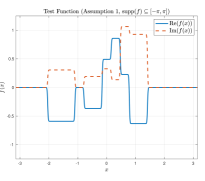
(a) Test Function (with ${\rm supp}(f)\subseteq[-\pi,\pi]$)

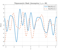
(b) Mask (Trigonometric Polynomial; $\rho=20$)

Figure 1: Representative Test Function and Mask Satisfying Assumption $1$.

To generate masks satisfying Assumption 1 (see Section 1.1), we choose the Fourier coefficients $\widehat{m}$ from a zero mean, unit variance i.i.d. complex Gaussian distribution and empirically verify that the mask-dependent constant $\mu_{1}$ (as defined in (16) is strictly positive. Fig. 1(b) plots such a (complex) trigonometric mask for $\rho=20$, where $\rho+1$ is the (two-sided) bandwidth of the mask. Table 1 lists the empirically calculated $\mu_{1}$ values, and averaged over $100$ trials) for such masks. The left two columns of the table list $\mu_{1}$ for a fixed discretization size ($d=211$) and varying $\rho$; they show that $\mu_{1}$ is approximately constant for fixed $d$. The right two columns list $\mu_{1}$ values for fixed $\rho$ and varying $d$; they show $\mu_{1}$ decreases slowly with $d$ (roughly proportional to $1/d$). This verifies that constructing admissible (i.e., with $\mu_{1}\neq 0$) trigonometric masks as per Assumption 1 is indeed possible for reasonable values of $d$ and $\rho$.

($d=211,\rho)$	$\mu_{1}$ (Average over $100$ trials)	($d,\rho=50)$	$\mu_{1}$ (Average over $100$ trials)
$(211,20)$	$1.957\times 10^{-4}$	$(111,50)$	$4.825\times 10^{-4}$
$(211,40)$	$1.704\times 10^{-4}$	$(223,50)$	$1.560\times 10^{-4}$
$(211,60)$	$1.563\times 10^{-4}$	$(447,50)$	$6.199\times 10^{-5}$
$(211,80)$	$1.500\times 10^{-4}$	$(895,50)$	$2.162\times 10^{-5}$
$(211,100)$	$1.530\times 10^{-4}$	$(1791,50)$	$8.247\times 10^{-6}$

Table 1: Empirically evaluated $\mu_{1}$ values (mask constant) for Algorithm 1. (Fourier coefficients of mask chosen as i.i.d. complex standard normal entries. Left two columns show $\mu_{1}$ values for fixed $d$, right two columns show $\mu_{1}$ values for fixed $\rho$.)

Finding closed form analytical expressions for the integral in (3) is non-trivial. Therefore, we use numerical quadrature computations on an equispaced fine grid (of $10,001$ points) in $[-\pi,\pi]$ to generate phaseless measurements corresponding to (3) under both Assumptions 1 and 2.

We now investigate the noise robustness of Algorithm 1. For the results shown in Fig. 2(a) (where each data point is generated by averaging the results of $100$ trials), we add i.i.d. random (real) Gaussian noise to the phaseless measurements (3) at desired signal to noise ratios (SNRs). In particular, the noise matrix $\mathbf{\bm{\eta}_{K,L}}\in\mathbbm{R}^{d\times L}$ in Section 3 is chosen to be i.i.d. $\mathcal{N}(\mathbf{0},\sigma^{2}\mathbf{I})$. The variance $\sigma^{2}$ is chosen such that

$$\mbox{SNR (dB)}=10\log_{10}\left(\frac{\|\mathbf{Z}\|_{F}^{2}}{dL\,\sigma^{2}}\right)$$

where $\mathbf{Z}$ denotes the corresponding matrix of perfect (noiseless) measurements. Errors in the recovered signal are also reported in dB with

$$\mbox{Error (dB)}=10\log_{10}\left(\frac{h\sum_{i=0}^{N}|f(x_{i})-f_{e}(x_{i})|^{2}}{h\sum_{i=0}^{N}|f(x_{i})|^{2}}\right),$$

where $f$ and $f_{e}$ denote the true and recovered functions respectively, and $x_{i}$ denotes (equispaced) grid points in $[-\pi,\pi]$, i.e. $x_{i}=-\pi+hi$ with $h\coloneqq 2\pi/N$. Errors reported in this section use $N=2003$.

Fig. 2(a) plots the error in recovering a test function using Algorithm 1 (for $d=257,\rho=32,\kappa=\rho-1$ and $(2\rho-1)d$ total measurements) over a wide range of SNRs. For reference, we also include results using an improved reconstruction method based on Algorithm 1, as well as the popular HIO+ER alternating projection algorithm [5, 11, 21]. Refinements over Algorithm 1 included use of an improved eigenvector-based magnitude estimation procedure in place of Step 6 (see [18, Section 6.1] for details), and (exponential) low-pass filtering in the output Fourier partial sum reconstruction step of Algorithm 1. The HIO+ER algorithm implementation used the zero vector as an initial guess, although use of a random starting guess did not change the qualitative nature of the results. As is common practice, (see for example [11]) we implemented the HIO+ER algorithm in blocks of eight HIO iterations followed by two ER iterations in order to accelerate convergence of the algorithm. To minimize computational cost while ensuring convergence (see Fig. 4), the total number of HIO+ER iterations was limited to $30$. As we see, Algorithm 1 compares well with the popular HIO+ER algorithm, with the improved method offering even better noise performance. Furthermore, this post-processing procedure does not significantly increase the computational cost. Fig. 2(b) plots the execution time (in seconds, averaged over $100$ trials) to recover a test signal using $dL$ measurements, where $d$ is the discretization size, $L=2\rho-1$ and $\rho=\min\{(d-5)/2,2\lfloor\log_{2}(d)\rfloor\}$. Both Algorithm 1 and its refined variant are essentially $\mathcal{O}(dL)$, where $dL$ is the number of measurements acquired, with Algorithm 1 performing much faster than the HIO+ER procedure. Finally, we note that reconstruction error can be reduced by increasing the number of shifts $L$ acquired (and consequently, the total number of measurements). Fig. 2(c) plots the error in reconstructing a test signal discretized using $d=257$ points, $\kappa=\rho-1$ and $Ld=(2\rho-1)d$ measurements for different values of $\rho$ (and correspondingly $L$). As expected, we see that noise performance improves as $L$ increases. Additional numerical experiments studying the convergence behavior of Algorithm 1 (in the absence of measurement errors) can be found in Appendix D.

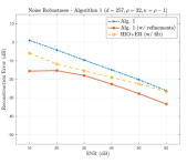
(a) Noise Robustness

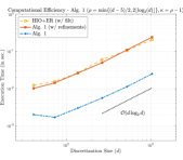
(b) Computational Cost

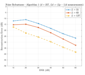
(c) Error vs. No. of Shifts

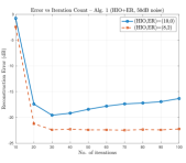
(d) HIO+ER Iterations

Figure 2: Empirical Evaluation of Algorithm 1 and Selection of HIO+ER Parameters for Comparison

5.2 Empirical Evaluation of Algorithm 2

We next present empirical simulations evaluating the robustness and efficiency of Algorithm 2. As detailed in Assumption 2 (see Section 1.1), we recover compactly supported test functions with $\operatorname{supp}(f)\subseteq(-a,a)$ using compactly supported masks which satisfy $\operatorname{supp}(\widetilde{m})\subseteq(-b,b)$, where $a+b<\pi$. For experiments in this section, we choose $b=3/4$ and $a=0.9(\pi-3/4)$. The test functions are generated as detailed in (44) of Section 5.1, as a (complex) weighted sum of shifted $C^{\infty}$-smooth bump functions, but with a maximum shift of $\nu_{{\rm max}}=a-b$. A representative test function is plotted in Fig. 3(a). The corresponding compactly supported masks are generated as the product of a trigonometric polynomial and a bump function using

$$\widetilde{m}(x)=\xi_{-b.b}(x)\cdot\left(\sum_{p=-\rho/2}^{\rho/2}\widehat{m}(p)\mathbbm{e}^{\mathbbm{i}px/b}\right),$$ (45)

where $\xi_{-b,b}$ is the $C^{\infty}$-smooth bump function described in Section 5.1, and the term in the parenthesis describes a (complex) $2b$-periodic trigonometric polynomial. A representative example of such as mask is provided in Fig. 3(b) with $\rho=16$ and the coefficients $\widehat{m}$ chosen from a zero mean, unit variance i.i.d. complex Gaussian distribution.

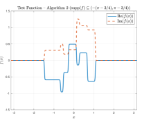
(a) Test Function ($a=\pi-3/4$; ${\rm supp}(f)\subseteq(-a,a))$

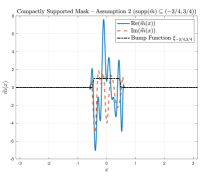
(b) Mask (${\rm supp}(\widetilde{m})\subseteq(-b,b)=(-3/4,3/4)$)

Figure 3: Representative Test Function and Mask Satisfying Assumption $2$.

($d=189,\kappa)$	$\mu_{2}$ (Average over $100$ trials)	($d,\kappa=27)$	$\mu_{2}$ (Average over $100$ trials)
$(189,3)$	$2.563\times 10^{-3}$	$(165,27)$	$9.722\times 10^{-5}$
$(189,10)$	$2.873\times 10^{-4}$	$(223,27)$	$8.866\times 10^{-5}$
$(189,31)$	$8.331\times 10^{-5}$	$(495,27)$	$4.686\times 10^{-5}$
$(189,94)$	$2.642\times 10^{-19}$	$(1045,27)$	$2.448\times 10^{-5}$

Table 2: Empirically evaluated $\mu_{2}$ values (mask constant) for Algorithm 2. The left two columns show $\mu_{2}$ values for fixed $d$, right two columns show $\mu_{2}$ values for fixed $\kappa$. Here, $\delta=\kappa+1$ and $s=\kappa-1$.

Representative values of the mask constant $\mu_{2}$ (as defined in (29) and averaged over $100$ trials) are listed in Table 2. The first two columns list $\mu_{2}$ values for fixed discretization size $d$, while the last two columns list $\mu_{2}$ values for fixed $\kappa$. In both cases, we set $K=2\kappa+1$ and ensure that $K$ divides $d$. We note that $\kappa$ denotes the number of modes used in the Wigner deconvolution procedure (Step $2$) in Algorithm 2. Since the masks constructed using (45) are compactly supported and smooth, we expect the autocorrelation of their Fourier transforms (and the corresponding Fourier coefficients of this autocorrelation) to decay rapidly. Therefore, we expect $\mu_{2}$ to be small for large $\kappa$ values; indeed, this is seen in the last row of Table 2 where the $\mu_{2}$ value is essentially zero when $d=189,\kappa=94$. However, as the functions we expect to recover also exhibit rapid decay in Fourier coefficients, we only require a small number of their Fourier modes to ensure accurate reconstructions. Hence, small to moderate $\kappa$ values suffice. As seen in Table 2, it is feasible to construct admissible masks (i.e., $\mu_{2}>0$) for such $(d,\kappa)$ pairs. Experiments have also been conducted with $\widetilde{m}$ chosen to be the bump function $\xi_{-b,b}$ and a (truncated) Gaussian, However, these experiments yield smaller mask constants $\mu_{2}$, which make the resulting reconstructions more susceptible to noise. Selection of “optimal” and physically realizable compactly supported masks is an open problem which we defer to future research.

We note that due to the equivalence of (27) and (28), the Wigner deconvolution step (Step $2$) in Algorithm 2 may be instead evaluated using (27). While theoretical analysis of this equivalent procedure is more involved, it offers computational advantages since it does not require solving the Vandermonde system of Step $4$ in Algorithm 2. The corresponding $\mu_{2}$ values for this procedure also follow the qualitative behavior in Table 2. This variant of Algorithm 2 is used in generating some of the plots in Appendix D, while Fig. 4 provides a comparison of Algorithm 2 and this alternate implementation.

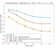
(a) Noise Robustness

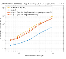
(b) Computational Cost

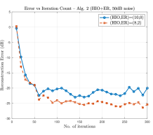
(c) HIO+ER Iterations

Figure 4: Empirical Evaluation of Algorithm 2 and Selection of HIO+ER Parameters for Comparison

We now study the robustness and computational efficiency of Algorithm 2. Fig. 4(a) plots the error in recovering a test function (with each data point averaged over $100$ trials) for discretization size $d=189$, $\delta=32$, $\kappa=\delta-1$, $s=29$ and $d/3$ total measurements over a wide range of SNRs. For reference, we also include results using the HIO+ER alternating projection algorithm, as well as the alternate implementation of Algorithm 2 (using (27) to implement the Wigner deconvolution Step $2$). As in Section 5.1, the alternate implementation of Algorithm 2 and the HIO+ER implementations utilize (exponential) low-pass filtering. The HIO+ER algorithm is implemented in blocks of eight HIO iterations followed by two ER iterations in order to accelerate the convergence of the algorithm, with a total of $100$ iterations used to ensure convergence while minimizing computational cost (see Fig. 4(c)). The proposed method (especially the alternate implementation) compares well with the HIO+ER algorithm. Additionally, we also provide results using a post-processed implementation of Algorithm 2 using just $10$ iterations of HIO+ER. In this context, we can view the proposed method as an initializer which accelerates the convergence of alternating projection algorithms such as HIO+ER. Finally, Fig. 4(b), which plots the execution time (in seconds, averaged over $100$ trials) to recover a test signal, shows that the proposed method in Algorithm 2 and its alternate implementation are computationally efficient, with all implementations running in $\mathcal{O}(dK)$ time where $dK$ is the number of measurements acquired.

Appendix A The Proofs of Lemmas 2 and 3

The Proof of Lemma 2.

We first note that $\|g\|_{L^{\infty}([-\pi,\pi])}<\infty$ since $g$ is a continuous periodic function. Next, we see that since $g$ is $C^{k}$-smooth, we have $|\widehat{g}(\omega)|\leq C_{g}\left(\frac{1}{|\omega|}\right)^{k}$ for all $\omega\in\mathbb{Z}\setminus\{0\}$, where $C_{g}$ is a constant which depends on only $g$ and $k$. As a result, we have

$$\|P_{\mathcal{A}}g\|_{L^{\infty}([-\pi,\pi])}\leq\sum_{\omega\in\mathbb{Z}}|\widehat{g}(\omega)|\leq|\widehat{g}(0)|+2C_{g}\sum_{m=1}^{\infty}\frac{1}{m^{k}}=C_{g}.$$

Similarly,

$$\|g-P_{\mathcal{N}}g\|_{L^{\infty}([-\pi,\pi])}\leq\sum_{|\omega|\geq\frac{n+1}{2}}|\widehat{g}(\omega)|\leq 2C_{g}\sum_{|\omega|\geq\frac{n+1}{2}}\left(\frac{1}{|\omega|}\right)^{\ell}\leq C_{g}\left(\frac{1}{n}\right)^{\ell-1}.$$

The desired result now follows. ∎

The Proof of Lemma 3.

Let $g\coloneqq P_{\mathcal{S}}f$ and $h\coloneqq P_{\mathcal{R}}m$, where $P_{\mathcal{S}}$ and $P_{\mathcal{R}}$ are the Fourier projection operators defined as in (6). Since $g$ and $h$ are trigonometric polynomials and $\mathcal{R}+\mathcal{S}\subseteq\mathcal{D}$, we may write

$$\int_{-\pi}^{\pi}g(x)h(x-\tilde{\ell})\mathbbm{e}^{-\mathbbm{i}x\omega}dx =\sum_{m\in\mathcal{R}}\sum_{n\in\mathcal{S}}\widehat{g}(n)\widehat{h}(m)\mathbbm{e}^{-\mathbbm{i}m\tilde{\ell}}\int_{-\pi}^{\pi}\mathbbm{e}^{\mathbbm{i}(m+n-\omega)x}dx$$

$$=\sum_{m\in\mathcal{R}}\sum_{n\in\mathcal{S}}\widehat{g}(n)\widehat{h}(m)\mathbbm{e}^{-\mathbbm{i}m\tilde{\ell}}\frac{2\pi}{d}\sum_{p\in\mathcal{D}}\mathbbm{e}^{2\pi\mathbbm{i}p(n+m-\omega)/d}$$

$$=\frac{2\pi}{d}\sum_{p\in\mathcal{D}}\left(\sum_{n\in\mathcal{S}}\widehat{g}(n)\mathbbm{e}^{2\pi\mathbbm{i}pn/d}\right)\left(\sum_{m\in\mathcal{R}}\widehat{h}(m)\mathbbm{e}^{\left(\left(\frac{2\pi\mathbbm{i}m}{d}\right)\left(p-\ell\right)\right)}\right)\mathbbm{e}^{-2\pi\mathbbm{i}mp\omega/d}$$

$$=\frac{2\pi}{d}\sum_{p\in\mathcal{D}}g\left(\frac{2\pi p}{d}\right)h\left(\frac{2\pi(p-\ell)}{d}\right)\mathbbm{e}^{-2\pi\mathbbm{i}p\omega/d}$$

$$=\frac{2\pi}{d}\sum_{p\in\mathcal{D}}x_{p}y_{p-\ell}\mathbbm{e}^{-2\pi\mathbbm{i}\omega p/d}.$$

∎

Appendix B The Proofs of Propositions 1 and 2

The Proof of Proposition 1.

We first note that

$$\widehat{z}_{q}=\begin{cases}\widehat{m}(q)&\text{if }|q|\leq\rho/2,\\ 0&\text{if }|q|>\rho/2.\end{cases}$$

Therefore, for all $|p|\leq\kappa-1$, we have

$$\left(\widehat{\mathbf{z}}\circ S_{p}\overline{\widehat{\mathbf{z}}}\right)_{q}=\begin{cases}\widehat{m}(q)\widehat{m}(p+q)&\text{if }-\rho/2\leq q,\,p+q\leq\rho/2,\\ 0&\text{otherwise}.\end{cases}$$

For any $|p|\leq\kappa-1,$ let

$$\mathcal{I}_{p}\coloneqq\{q\in\mathcal{D}:-\rho/2\leq q\leq\rho/2\quad\text{and }-\rho/2\leq q+p\leq\rho/2\}.$$

One may check that

$$\mathcal{I}_{p}=\begin{cases}\left[-\frac{\rho}{2}-p,\frac{\rho}{2}\right]\cap\mathbb{Z}&\text{if }p<0\\ \left[-\frac{\rho}{2},\frac{\rho}{2}-p\right]\cap\mathbb{Z}&\text{if }p\geq 0\end{cases}.$$

Therefore, making a simple change of variables in the case $p<0,$ we have that

$$\mathbf{F_{d}}\left(\widehat{\mathbf{z}}\circ S_{p}\overline{\widehat{\mathbf{z}}}\right)_{q} =\frac{1}{d}\sum_{\ell\in\mathcal{I}_{p}}\widehat{m}(\ell)\widehat{m}(p+\ell)\mathbbm{e}^{-2\pi\mathbbm{i}q\ell/d}=\frac{1}{d}\sum_{\ell=-\rho/2}^{\rho/2-|p|}\widehat{m}(\ell)\widehat{m}\left(\ell+|p|\right)\mathbbm{e}^{\mathbbm{i}\phi_{p,q,\ell}},$$

where $\mathbbm{e}^{\mathbbm{i}\phi_{p,q,\ell}}$ is a unimodular complex number depending on $p,q$ and $\ell.$ Using the assumptions (17) and (18), we see that

$$\bigg{|}\frac{1}{d}\sum_{\ell=-\rho/2+1}^{\rho/2-|p|}\widehat{m}(\ell)\widehat{m}(\ell+|p|)\mathbbm{e}^{\mathbbm{i}\phi_{p,q,\ell}}\bigg{|} \leq\frac{\rho}{d}\left|\widehat{m}\left(\frac{-\rho}{2}+1\right)\right|\left|\widehat{m}\left(\frac{-\rho}{2}+1+|p|\right)\right|$$

$$\leq\frac{1}{2d}\left|\widehat{m}\left(\frac{-\rho}{2}\right)\right|\left|\widehat{m}\left(\frac{-\rho}{2}+|p|\right)\right|.$$

With this, we may use the reverse triangle inequality to see

$$\bigg{|}\mathbf{F_{d}}\left(\widehat{\mathbf{z}}\circ S_{p}\overline{\widehat{\mathbf{z}}}\right)_{q}\bigg{|} =\bigg{|}\frac{1}{d}\sum_{\ell=-\rho/2}^{\rho/2-|p|}\widehat{m}(\ell)\widehat{m}(\ell+|p|)\mathbbm{e}^{\mathbbm{i}\phi_{p,q,\ell}}\bigg{|}$$

$$\geq\frac{1}{d}\bigg{|}\widehat{m}\left(\frac{-\rho}{2}\right)\bigg{|}\left|\widehat{m}\left(\frac{-\rho}{2}+|p|\right)\right|-\frac{1}{d}\bigg{|}\sum_{\ell=-\rho/2+1}^{\rho/2-|p|}\widehat{m}(\ell)\widehat{m}(\ell+|p|)\mathbbm{e}^{\mathbbm{i}\phi_{p,q,\ell}}\bigg{|}$$

$$\geq\frac{1}{2d}\left|\widehat{m}\left(\frac{-\rho}{2}\right)\right|\left|\widehat{m}\left(\frac{-\rho}{2}+|p|\right)\right|$$

$$\geq\frac{1}{2d}\left|\widehat{m}\left(\frac{-\rho}{2}\right)\right|\left|\widehat{m}\left(\frac{-\rho}{2}+\kappa-1|\right)\right|.$$

∎

The Proof of Proposition 2.

First, we note that by applying Lemma 5, and setting $p=\omega,q=\ell$, we have

$$\mu_{2}=\inf_{\omega\in[2\kappa-1]_{c},\ell\in[2s-1]_{c}}|(\mathbf{F_{d}}(\widehat{\mathbf{z}}\circ S_{\ell}\overline{\widehat{\mathbf{z}}}))_{\omega}|=\frac{1}{d}\inf_{\omega\in[2\kappa-1]_{c},\ell\in[2s-1]_{c}}|(\mathbf{F_{d}}(\mathbf{z}\circ S_{\omega}\overline{\mathbf{z}}))_{\ell}|=\frac{1}{d}\inf_{p\in[2\kappa-1]_{c},q\in[2s-1]_{c}}|(\mathbf{F_{d}}(\mathbf{z}\circ S_{p}\overline{\mathbf{z}}))_{q}|.$$

For $|p|\leq\kappa-1$, we have

$$\left(\mathbf{z}\circ S_{p}\overline{\mathbf{z}}\right)_{q}=\begin{cases}z_{q}\overline{z_{p+q}}&\text{if }n\leq q,p+q\leq n+\tilde{\delta}-1,\\ 0&\text{otherwise}.\end{cases}$$

For any $|p|\leq\kappa-1,$ let

$$\mathcal{I}_{p}\coloneqq\{q\in\mathcal{D}:n\leq q\leq n+\tilde{\delta}-1\quad\text{and}\quad n\leq q+p\leq n+\tilde{\delta}-1\}.$$

One may check that

$$\mathcal{I}_{p}=\begin{cases}[n-p,n+\tilde{\delta}-1]\cap\mathbb{Z}&\text{if }p<0,\\ [n,n+\tilde{\delta}-1-p]\cap\mathbb{Z}&\text{if }p\geq 0.\end{cases}$$

Therefore, making a simple change of variables in the case $p<0,$ we have that in either case

$$\left|\mathbf{F_{d}}\left(\mathbf{z}\circ S_{p}\overline{\mathbf{z}}\right)_{q}\right| =\frac{1}{d}\bigg{|}\sum_{\ell\in\mathcal{I}_{p}}z_{\ell}\overline{z_{p+\ell}}\mathbbm{e}^{-2\pi\mathbbm{i}\ell q/d}\bigg{|}=\frac{1}{d}\bigg{|}\sum_{\ell=n}^{n+\tilde{\delta}-1-|p|}z_{\ell}\overline{z_{\ell+|p|}}\mathbbm{e}^{\mathbbm{i}\phi_{p,q,\ell}}\bigg{|},$$

where $\mathbbm{e}^{\mathbbm{i}\phi_{p,q,\ell}}$ is a unimodular complex number depending on $p,q$ and $\ell.$ Using the assumptions (30) and (31) we see that

$$\bigg{|}\frac{1}{d}\sum_{\ell=n+1}^{n+\tilde{\delta}-1-|p|}z_{\ell}\overline{z_{\ell+|p|}}\mathbbm{e}^{\mathbbm{i}\phi_{p,q,\ell}}\bigg{|}\leq\frac{\tilde{\delta}}{d}\left|z_{n+1}\right|\left|z_{n+1+|p|}\right|\leq\frac{1}{2d}|z_{n}||z_{n+|p|}|.$$

With this,

$$\left|F_{d}\left(\mathbf{z}\circ S_{p}\overline{\mathbf{z}}\right)_{q}\right| =\bigg{|}\frac{1}{d}\sum_{\ell=n}^{n+\tilde{\delta}-1-|p|}z_{\ell}\overline{z_{\ell+|p|}}\mathbbm{e}^{\mathbbm{i}\phi_{p,q,\ell}}\bigg{|}\geq\frac{1}{d}|z_{n}||z_{n+|p|}|-\bigg{|}\frac{1}{d}\sum_{\ell=n+1}^{n+\tilde{\delta}-1-|p|}z_{\ell}\overline{z_{\ell+|p|}}\mathbbm{e}^{\mathbbm{i}\phi_{p,q,\ell}}\bigg{|}$$

$$\geq\frac{1}{2d}|z_{n}||z_{n+|p|}|\geq\frac{1}{2d}|z_{n}||z_{n+\kappa-1}|.$$

∎

Appendix C The Proof of Lemma 7

Proof.

Our proof requires the following sublemma which shows that, if $n\in L_{f}$, then Algorithm 3 used in the definition of $\alpha_{n}$ will only select indices $n_{\ell}$ corresponding to large Fourier coefficients.

Lemma 8.

Let $n\in L_{f}$, and let $n_{0},\ldots,n_{b}$ be the sequence of indices as introduced in the definition of $\alpha_{n}$. Then

$$|\widehat{f}(n_{\ell})|\geq\frac{|\widehat{f}(n)|}{2}$$

for all $0\leq\ell\leq b$.

Proof.

When $\ell=b$, the claim is immediate from the fact that $n_{b}=n$. For all $0\leq\ell\leq b-1$, the definition of $n_{\ell}$ implies that there exists an interval $I_{\ell}$ of length $\beta$, which is centered at some point $a$ with $|a|\leq|n|$, such that

$$a_{n_{\ell}}=\max_{m\in I_{\ell}}a_{m}.$$

Letting $\epsilon=\sqrt{3\|\mathbf{N}\|_{\infty}}$, we see that by (38) and Remark 1

$$|\widehat{f}(n_{\ell})| \geq a_{n_{\ell}}-\epsilon=\max_{m\in I_{\ell}}a_{m}-\epsilon\geq\max_{m\in I_{\ell}}|\widehat{f}(m)|-2\epsilon\geq|\widehat{f}(n)|-2\epsilon.$$

The result now follows from noting that $\epsilon<\frac{|\widehat{f}(n)|}{4}$ for all $n\in L_{f}$. ∎

With Lemma 8 established, we may now prove Lemma 7. Let $n\in L_{f}$ and let $n_{0},\ldots n_{b}$ be the sequence describe in the definition of $\alpha_{n}$. For $0\leq\ell\leq b-1$, let $t_{\ell}\coloneqq\widehat{f}(n_{\ell+1})\overline{\widehat{f}(n_{\ell})}$, $a^{\prime}_{\ell}\coloneqq\widehat{f}(n_{\ell+1})\overline{\widehat{f}(n_{\ell})}+N_{n_{\ell+1},n_{\ell}}$, and $N^{\prime}_{\ell}\coloneqq N_{n_{\ell+1},n_{\ell}}$. Consider the triangle with sides $a^{\prime}_{\ell}$, $t_{\ell}$, and $N^{\prime}_{\ell}$ with angles $\theta_{\ell}=|\arg(a^{\prime}_{\ell})-\arg(t_{\ell})|$ and $\phi_{\ell}=|\arg(a^{\prime}_{\ell})-\arg(N^{\prime}_{\ell})|$, as illustrated in Figure 5.

Figure 5: Triangle in the complex domain.

By the law of sines and Lemma 8, we get that

$$|\sin(\theta_{\ell})|=\left|\frac{N_{\ell}^{\prime}}{t_{\ell}}\sin(\phi_{\ell})\right|\leq\frac{\|\mathbf{N}\|_{\infty}}{|\widehat{f}(n_{\ell})||\widehat{f}(n_{\ell+1})|}\leq\frac{4\|\mathbf{N}\|_{\infty}}{|\widehat{f}(n)|^{2}}$$ (46)

for all $0\leq\ell\leq b$. By the definition of $L_{f}$ and Lemma 8, we have that for all $\ell$

$$|N^{\prime}_{\ell}|\leq\|\mathbf{N}\|_{\infty}\leq\frac{|\widehat{f(n)}|^{2}}{4}\leq|\widehat{f}(n_{\ell})||\widehat{f}(n_{\ell+1})|=|t_{\ell}|.$$

Therefore, $0\leq\theta_{\ell}\leq\frac{\pi}{2}$, and so by (46), we have

$$|\theta_{\ell}|\leq\frac{\pi}{2}\,|\sin(\theta_{\ell})|\leq 2\pi\,\frac{\|\mathbf{N}\|_{\infty}}{|\widehat{f}(n)|^{2}}.$$

By definition $\tau_{n}=\sum_{\ell=0}^{b-1}\arg(t_{\ell})$ and $\alpha_{n}=\sum_{l=0}^{b-1}\arg(a^{\prime}_{\ell})$. Therefore, we have

$$|\mathbbm{e}^{\mathbbm{i}\tau_{n}}-\mathbbm{e}^{\mathbbm{i}\alpha_{n}}|\leq|\alpha_{n}-\tau_{n}| =\bigg{|}\sum_{\ell=0}^{b-1}\arg(a^{\prime}_{\ell})-\arg(t_{\ell})\bigg{|}=\bigg{|}\sum_{\ell=0}^{b-1}\theta_{\ell}\bigg{|}\leq 2\pi b\frac{\|\mathbf{N}\|_{\infty}}{|\widehat{f}(n)|^{2}}.$$

From the definition of $n_{\ell}$, we have

$$|n_{\ell}-n_{\ell-1}|\geq\gamma-\beta\geq\frac{\gamma}{2}$$

for all $1\leq\ell\leq b-1$. Therefore, the path length $b$ is bounded by

$$b\leq\frac{|n-n_{0}|}{\min|n_{\ell}-n_{\ell-1}|}\leq\frac{2d}{\gamma}.$$

Thus, we have

$$|\mathbbm{e}^{\mathbbm{i}\tau_{n}}-\mathbbm{e}^{\mathbbm{i}\alpha_{n}}|\leq 2\pi b\frac{\|\mathbf{N}\|_{\infty}}{|\widehat{f}(n)|^{2}}\leq\frac{4\pi d}{\gamma}\frac{\|\mathbf{N}\|_{\infty}}{|\widehat{f}(n)|^{2}}$$

as desired.

∎

Appendix D Additional Numerical Simulations using Algorithms 1 and 2

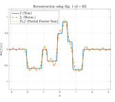
(a) $d=33$

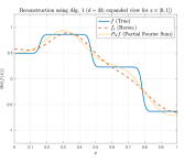
(b) $d=33$ (zoom)

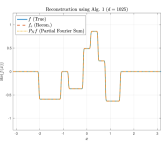
(c) $d=1025$

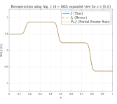
(d) $d=1025$ (zoom)

Figure 6: Evaluating the convergence behavior of Algorithm 1. Figure plots reconstructions of the real part of the test function at $d=33$ and $d=1025$ (along with an expanded view of the reconstruction in $[0,1]$) on a discrete equispaced grid in $[-\pi,\pi]$ of $7003$ points; we set $\rho=\min\{(d-5)/2,16\lfloor\log_{2}(d)\rfloor\}$ and $\kappa=\rho-1$.

In this section, we provide additional numerical simulations studying the empirical convergence behavior of Algorithms 1 and 2. We start with a study of the convergence behavior of Algorithm 1. Here, we reconstruct the same test function using different discretization sizes $d$ (with $\rho$ chosen to be $\min\{(d-5)/2,16\lfloor\log_{2}(d)\rfloor\}$ and $\kappa=\rho-1$), where the total number of phaseless measurements used is $Ld=(2\rho-1)d$. Fig. 6 plots representative reconstructions (of the real part of the test function) for two choices of $d$ ($d=33$ and $d=1025$). We note that the (smooth) test function illustrated in the figure has several sharp and closely separated gradients, making the reconstruction process challenging. This is evident in the partial Fourier sums ($P_{N}f$) plotted for reference alongside the reconstructions from Algorithm 1 ($f_{e}$). For small $d$ and $\rho$, we observe oscillatory behavior similar to that seen in the Gibbs phenomenon. Nevertheless, we see that the proposed algorithm closely tracks the performance of the partial Fourier sum, with reconstruction quality improving significantly as $d$ (and $\rho$) increases.

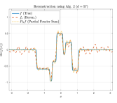
(a) $d=57$

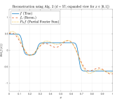
(b) $d=57$ (zoom)

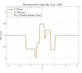
(c) $d=921$

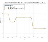
(d) $d=921$ (zoom)

Figure 7: Evaluating the convergence behavior of Algorithm 2. Figure plots reconstructions of the real part of the test function at $d=57$ and $d=921$ (along with an expanded view of the reconstruction in $[0,1]$) on a discrete equispaced grid in $[-\pi,\pi]$ of $7003$ points; we set $K=d/3,\delta=(K+1)/2$ and $\kappa=\delta-1$.

We next evaluate the convergence behavior of Algorithm 2 by reconstructing the same test function using different discretization sizes $d$ (with $K=d/3$, $\delta=(K+1)/2$, $\kappa=\delta-1$ and $s=\kappa-1$). Fig. 7 plots representative reconstructions (of the real part of the test function) for two choices of $d$ ($d=57$ and $d=921$). As in Fig. 6, we note that the (smooth) test function has several sharp and closely separated gradients, making the reconstruction process challenging. Again, the partial Fourier sums ($P_{N}f$) plotted alongside the reconstructions from Algorithm 2 ($f_{e}$) exhibit Gibbs-like oscillatory behavior for small $d$ and $\kappa$. Nevertheless, we see that the proposed algorithm closely tracks the performance of the partial Fourier sum, with reconstruction quality improving significantly as $d$ (and $\delta,\kappa$) increases.

References

- [1] Rima Alaifari, Ingrid Daubechies, Philipp Grohs, and Rujie Yin. Stable phase retrieval in infinite dimensions. Foundations of Computational Mathematics, 19(4):869–900, 2019.
- [2] Rima Alaifari and Matthias Wellershoff. Uniqueness of stft phase retrieval for bandlimited functions. Applied and Computational Harmonic Analysis, 50:34 – 48, 2021.
- [3] B. Alexeev, A. S. Bandeira, M. Fickus, and D. G. Mixon. Phase Retrieval with Polarization. SIAM Journal on Imaging Sciences, 7(1):35–66, 2014.
- [4] Radu Balan, Pete Casazza, and Dan Edidin. On signal reconstruction without phase. Applied and Computational Harmonic Analysis, 20(3):345–356, 2006.
- [5] Heinz H Bauschke, Patrick L Combettes, and D Russell Luke. Phase retrieval, error reduction algorithm, and Fienup variants: A view from convex optimization. Journal of the Optical Society of America. A, Optics, Image science, and Vision, 19(7):1334–1345, 2002.
- [6] Alessandro Buccini, Marco Donatelli, and Lothar Reichel. Iterated tikhonov regularization with a general penalty term. Numerical Linear Algebra with Applications, 24(4):2089, 2017.
- [7] Emmanuel J Candès, Yonina C Eldar, Thomas Strohmer, and Vladislav Voroninski. Phase retrieval via matrix completion. SIAM review, 57(2):225–251, 2015.
- [8] Emmanuel J. Candès, Xiaodong Li, and Mahdi Soltanolkotabi. Phase retrieval from coded diffraction patterns. Applied and Computational Harmonic Analysis, 39(2):277 – 299, 2015.
- [9] Cheng Cheng, Ingrid Daubechies, Nadav Dym, and Jianfeng Lu. Stable phase retrieval from locally stable and conditionally connected measurements. arXiv preprint arXiv:2006.11709, 2020.
- [10] C Fienup and J Dainty. Phase retrieval and image reconstruction for astronomy. Image Recovery: Theory and Application, pages 231–275, 1987.
- [11] James R Fienup. Phase retrieval algorithms: a comparison. Applied optics, 21(15):2758–2769, 1982.
- [12] F. Filbir, F. Krahmer, and O. Melnyk. On recovery guarantees for angular synchronization. arXiv preprint arXiv 2005.02032, 2020.
- [13] A. Forstner, F. Krahmer, O. Melnyk, and N. Sissouno. Well conditioned ptychograpic imaging via lost subspace completion. Inverse Problems, 2020. arXiv preprint arXiv 2004.04458.
- [14] R.W. Gerchberg and W.O. Saxton. A Practical Algorithm for the Determination of Phase from Image and Diffraction Plane Pictures. Optik, 35:237–246, 1972.
- [15] Daniel Griffin and Jae Lim. Signal estimation from modified short-time fourier transform. IEEE Transactions on Acoustics, Speech, and Signal Processing, 32(2):236–243, 1984.
- [16] Karlheinz Gröchenig. Phase-retrieval in shift-invariant spaces with gaussian generator. Journal of Fourier Analysis and Applications, 26, 2020.
- [17] David Gross, Felix Krahmer, and Richard Kueng. Improved recovery guarantees for phase retrieval from coded diffraction patterns. Applied and Computational Harmonic Analysis, 42:37 – 64, 2017.
- [18] M. A. Iwen, B. Preskitt, R. Saab, and A. Viswanathan. Phase retrieval from local measurements: improved robustness via eigenvector-based angular synchronization. Applied and Computational Harmonic Analysis, 48:415 – 444, 2020.
- [19] Mark A Iwen, Sami Merhi, and Michael Perlmutter. Lower Lipschitz bounds for phase retrieval from locally supported measurements. Applied and Computational Harmonic Analysis, 2019.
- [20] Mark A. Iwen, Aditya Viswanathan, and Yang Wang. Fast Phase Retrieval from Local Correlation Measurements. SIAM Journal on Imaging Sciences, 9(4):1655–1688, 2016.
- [21] Stefano Marchesini, Yu-Chao Tu, and Hau-tieng Wu. Alternating projection, ptychographic imaging and phase synchronization. Applied and Computational Harmonic Analysis, 41(3):815–851, 2016.
- [22] Michael Perlmutter, Sami Merhi, Aditya Viswanathan, and Mark Iwen. Inverting spectrogram measurements via aliased wigner distribution deconvolution and angular synchronization. Information and Inference: A Journal of the IMA, 2020.
- [23] JM Rodenburg. Ptychography and related diffractive imaging methods. Advances in Imaging and Electron Physics, 150:87–184, 2008.
- [24] Gaurav Thakur. Reconstruction of bandlimited functions from unsigned samples. J. Fourier Anal. Appl., 17(4):720–732, 2011.
- [25] Adriaan Walther. The question of phase retrieval in optics. Optica Acta: International Journal of Optics, 10(1):41–49, 1963.