New data structure for univariate polynomial approximation and applications to root isolation, numerical multipoint evaluation, and other problems
guillaume.moroz@inria.fr
November 17, 2021 )
Abstract
We present a new data structure to approximate accurately and efficiently a polynomial of degree given as a list of coefficients . Its properties allow us to improve the state-of-the-art bounds on the bit complexity for the problems of root isolation and approximate multipoint evaluation. This data structure also leads to a new geometric criterion to detect ill-conditioned polynomials, implying notably that the standard condition number of the zeros of a polynomial is at least exponential in the number of roots of modulus less than or greater than .
Given a polynomial of degree with for
, isolating all its complex roots or evaluating it at
points can be done with a quasi-linear number of arithmetic
operations. However, considering the bit complexity, the
state-of-the-art algorithms require at least bit operations
even for well-conditioned polynomials and when the accuracy required
is low. Given a positive integer , we can compute our new data
structure and evaluate at points in the unit disk with an
absolute error less than in bit
operations, where means that we omit logarithmic
factors. We also show that if is the absolute condition
number of the zeros of , then we can isolate all the roots of
in bit operations. Moreover, our
algorithms are simple to implement. For approximating the complex
roots of a polynomial, we implemented a small prototype in
Python/NumPy that is an order of magnitude faster than the
state-of-the-art solver MPSolve for high degree polynomials
with random coefficients.
Keywords: Polynomial evaluation, Complex root finding, Condition number
1 Introduction
One of the fundamental problem in computer algebra is the evaluation of polynomials. Since 1972, it is known that evaluating a univariate polynomial of degree on points can be done in a quasi-linear number of arithmetic operations [17]. Unfortunately, this bound doesn’t hold if we consider the bit complexity, where the arithmetic operations performed with a precision of bits costs bit operations. If we want to evaluate approximatively a polynomial on points up to a constant absolute error, a direct application of Fiduccia algorithm leads to a bit-complexity bound in bit operations, and a more sophisticated algorithm provides a bound in [45]. For almost 50 years, the following problem has remained open.
Given a polynomial of degree with coefficients of constant size, and complex points in the unit disk, is it possible to compute all the up to a constant absolute error with a number of bit operations quasi-linear in ?
Nevertheless, the evaluation of polynomials on multiple points is used in many areas of computer science, such as polynomial system solving with the Newton method [43, 24, 12, 8, 5], homotopy continuation [11, 10, 4, 31, 8] or subdivision algorithms [36, 29, 34], visualisation of algebraic surfaces through raytracing or mesh computation [47], among others. Speeding up the numerical evaluation of polynomials may lead to an effortless practical improvement for many existing algorithms.
We introduce in Sections 1.1 and 3 a new data structure, that allows us to finally solve this problem. It approximates the input polynomial by a piecewise polynomial on a carefully chosen domain that depends solely on the degree of the input polynomial, and the required precision. The fact that the domain is fixed and not adaptive makes it easy to implement.
Moreover, we show that our new data structure improves not only the
bound for the numeric multipoint evaluation problem
(Sections 1.2.1 and 4), but also the bound
for the root isolation problem (Sections 1.2.2
and 5), and the lower bound on the condition
number of polynomials (Sections 1.2.3
and 6). We expect that our approach will lead further
improvements for other related problems, notably multivariate polynomial
evaluation and polynomial system solving. As a proof of concept, we also
implemented the root isolation algorithm presented in this article. Even
though our implementation is less than lines of code written in
Python, it is an order of magnitude faster than the
state-of-the-art optimized implementation MPSolve for high degree
polynomials with random coefficients (Section 1.2.4
and source code in Appendix A).
1.1 The data structure
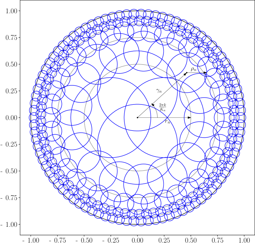
Given a polynomial of degree and an integer , we will introduce in Definition 2 the so-called an -hyperbolic approximation of , which can be seen as a piecewise approximation of by polynomials of degree . The key that will allow us to improve the state-of-the-art complexity bounds of several classical problems related to univariate complex polynomials is the hyperbolic layout used to compute this piecewise approximation. We first define this layout so-called hyperbolic covering, illustrated in Figure 1. Roughly, a hyperbolic covering is a set of disks of radius exponentially smaller near the unit circle, and such that their union contains the unit disk.
Definition 1.
Given a positive integer , an -hyperbolic covering of the unit disk is the set of disks of centers and radii for and , where and are defined by:
Remark 1.
We can also write explicitly the corresponding sequences and :
We also have explicitly , using and .
We will see in Lemma 3 that for all integers , the union of the disks of a -hyperbolic covering contains the unit disk.We can now define the -hyperbolic approximation of a polynomial , that can be seen as piecewise approximation of by polynomials of degree lower than .
Definition 2.
Given a polynomial of degree with , and an integer , an -hyperbolic approximation of is a finite set of pairs , where is a polynomial of degree , with coefficients of bit size , and is an affine transform, such that:
-
•
the set of disks is the -hyperbolic covering with
-
•
Since we constrain the polynomials approximating to have a degree , that can be significantly smaller than , it is not obvious that an approximation satisfying the conditions defined above always exists. The following theorem proves that it always exists, and furthermore that it can be computed in quasi-linear time with respect to the degree of .
Theorem 1.
Let be a polynomial of degree with , and be an integer. Algorithm 1 computes an -hyperbolic approximation of , denoted by , in bit operations.
Remark also that the maximal precision required for the arithmetic operations in Algorithm 1 is in , which makes it suitable for an implementation with machine precision arithmetic.
Main idea of the proof of Theorem 1.
Denoting the center and the radius of a disk in a -hyperbolic approximation by and , we need to prove that it is possible to compute a polynomial of degree that satisfies the bounds of Theorem 1. This comes from the fact that using the formula of Definition 1 and Remark 1, we can check that the coefficients of degree of the polynomial have a modulus less than for all . Then it remains to prove that we can approximate the first coefficients of all the in bit operations. For that, remark that . Thus, it is sufficient to prove that for a fixed , we can compute for all in bit operations. This can be done by using a combination of fast numerical composition of series (Proposition 3), and numerical fast Fourier transform (Proposition 2). More details can be found in Section 3.
1.2 Applications
Based on our new data structure, we describe three independent results that improve state-of-the-art solutions to long-standing problems. First we improve the complexity for evaluating numerically polynomials on multiple points. Then we improve the complexity of finding the roots of well-conditioned polynomials. Finally, we present a new lower bound on the condition number of the zeros of a polynomial, based on simple geometric properties of the distribution of its roots.
1.2.1 Numerical multipoint evaluation
In the literature [17, 2], [46, Chapter 10], a fast multipoint evaluation algorithm has been designed to evaluate points of a degree polynomial with a number of arithmetic operations quasi-linear in . However, in the case of numerical evaluation with precision after the binary point, this algorithm uses a number of bit operations quadratic in , even for a constant . This is due notably to the fact that this algorithm introduces intermediate polynomials with coefficients that may have a bit-size linear in . A careful analysis of the bit-complexity of this algorithm for numerical evaluation ([45, Lemma 11]) shows that this algorithm uses bit operations.
Specific sets of points were found where the problem of numeric multipoint evaluation can be solved in a quasi-linear time in . The most famous one is the set of roots of unity. Computing a numerical approximation of the for can be done in quasi-linear time [41] in . Another family of points was used by Ritzmann for the problem of fast numeric composition of series [39, Proposition 3.4]. He showed that if the modulus of the is lower than , then all the can be approximated numerically in a quasi-linear number of bit operations.
In a more recent work [45, §3.2], van der Hoeven gave the first sub-quadratic bound to evaluate points with modulus less than . More precisely, he showed that if it is possible to evaluate the with an error less than with bit operations. He achieved this bound by subdividing the unit disk in annuli of constant width. A drawback of this bound is that it increases the exponent on the required precision . By contrast, in our data structure, we subdivide the unit disk with disks of width exponentially smaller near the unit circle. This approach allows us to finally derive an algorithm that is both quasi-linear in and in for the numerical multipoint evaluation problem.
Theorem 2.
Given a polynomial of degree with , Algorithm 2 returns the evaluation of on points in the unit disk with an absolute error less than in bit operations.
Remark 2.
Using Algorithm 2 on the reverse polynomial , we see that the same complexity bound holds for a set of points in the complex plane, replacing by the function
Our algorithm is particularly well-suited for evaluating polynomials of high degree with fixed constant precision such as machine precision. This arises in many applications, notably in polynomial root approximation. One of the most famous method to approximate a root of a polynomial is the Newton method. Starting from an initial point , it consists in computing iteratively the Newton map, yielding the sequence . It was shown that starting from an explicit set of points, this approach is guaranteed to approximate all the roots of a given polynomial [24, 5]. In their work, the authors only show experiences with polynomial given by recursive formula, such that they can be evaluated with a number of operations logarithmic in their degree. Our data structure can improve their approach for dense polynomials given by their list of coefficients. In Section 1.2.2, we focus on the computation of disks isolating the roots of , that is the computation of a set of disks that are pairwise disjoint and that contain a unique root of each.
Main idea of the proof of Theorem 2.
Once we have computed a -hyperbolic approximation of the input polynomial , the algorithm is rather straight-forward. For each disk of the corresponding hyperbolic covering, we can efficiently find all the input points that it contains, using a geometric data-structure such as range searching, recalled in Section 2.7. Then, using the state-of-the-art algorithm for multipoint evaluation (Proposition 4), we can evaluate the corresponding approximate polynomial from the hyperbolic approximation on the selected points. Since has a degree lower than , evaluating on the up to precision can be done with an amortized time per point if the number of points is greater than and in a total time if there are less than points. Since the number of disks in a hyperbolic approximation is in , this leads to a bit complexity in . More details can be found in Section 4.
1.2.2 Root isolation
Our data structure also allows us to improve the state-of-the-art bound on the bit complexity for the problem of isolating all the complex roots of a given polynomial, with a bound that is adaptive in the condition number of the input. The condition number of the zeros of a polynomial measures the displacement of its roots with respect to a perturbation of its coefficients (Definition 3). For a square-free polynomial and a root , we let . Then the absolute condition number of is . Our goal is to provide for each root an isolating disk, that is a disk that contains a unique root and doesn’t intersect any other isolating disk. In our case we consider so-called projective disks, that is either a disk or the inverse of a disk defined as the set of points such that and .
Theorem 3.
Given a square-free polynomial of degree with , with absolute condition number , Algorithm 3 computes isolating projective disks of all the roots of in bit operations.
Remark 3.
If all the coefficients of are real numbers, then Algorithm 3 can be slightly modified to return all the real roots of with the same bit-complexity, by selecting the isolating projective disks that intersects the real axis.
In recent works on complex root isolation [33, 3], the best adaptive complexity bound, rewritten with our notation, is in , where . Our bound removes the dependency in , and replaces the sum by a max, which improves the state-of-the-art bounds by a factor if the condition numbers of the roots are logarithmic in or evenly distributed. In adaptive algorithms that compute isolating disks, a criterion is used for early termination. It usually checks if a disk or a rectangle contains a unique root of . Some examples of criteria are detailed in Section 2.6. All those criteria end up evaluating a polynomial of degree roughly on each of the roots ([33, §2.2.3],[3, Lemma 5], [26, Algorithms 2 and 3], …), which leads to a bit-complexity at least quadratic in if we use a naive evaluation algorithm, or in using state-of-the-art multipoint evaluation methods [45]. In our case, thanks to our new data structure, the criterion to check that a disk contains a unique root is replaced by the evaluation of a polynomial of degree , which explains partly how we avoid a cost quadratic in .
Another approach in the literature consists in computing the roots up to a precision high enough such that we can guarantee that all the roots are approximated correctly. An explicit bound exists in the case where the input polynomial has integer coefficients. Schönhage showed [42, §20]) that if we can compute an approximate factorization of close enough, then the roots of are isolated by disks centered on the roots of with a radius depending on the condition number . Combined with a bound on from Mahler [32, last inequality] for polynomials with integer coefficients, and using the algorithm of Pan [37] to compute the approximate factorization , this leads to a root-isolating algorithm in bit operations [16, §10.3.1]. Note that this algorithm requires arithmetic operations performed with a precision in , and requires at least a quadratic number of bit operations. This method was also improved in practice for small degree polynomials [20].
In our case, the bound from Mahler on implies that the bit complexity of Algorithm 3 is also in , matching the bit-complexity of state-of-the art algorithms in the worst case for square-free polynomials with integer coefficients.
Main idea of the proof of Theorem 3.
Our approach roughly follows the original approach of Schönhage [42, §20] in the sense that we will compute isolating disks centered on the roots of an approximation of . It is also adaptive like more recent works ([33, 3, 26], among others), in the sense that we use a criterion for early termination.
The main novelty of our approach is that we start by computing an -hyperbolic approximation of , for a small initial constant integer . This returns a set of polynomials of degree defined on disks covering the unit disk . Then we compute the approximate roots of the and we use a criterion to check if the corresponding approximate roots are the centers of disks isolating the roots of . If we did not find all the roots of , we double the parameter and we start again. The criterion that we use to check if an approximate root is the center of an isolating disk is based on Kantorovich theory (recalled in Section 2.6) and it can be tested using the approximate polynomials of degree lower than coming from the hyperbolic approximation. Moreover, this criterion will be satisfied for all roots of for for a universal constant (Lemma 8). Further details can be found in Section 5.
1.2.3 Lower bound on condition number
Another insightful application of our data structure is a new geometrical interpretation of ill-conditioned polynomials, based on the distribution of their roots. Since the introduction of Wilkinson’s polynomials , it is known that the problem of polynomial root finding can be ill-conditioned even in the cases where the roots are well separated [48, 49]. More recently, it has been proved that the condition number of characteristic polynomials of Gaussian matrices is in in average [9], where a Gaussian matrix is a matrix where the entries are independent, centered Gaussian random variables. Yet, no approaches provide a geometric explanation of this phenomenon. Our next theorem provides a geometric criterion that allows one to detect easily if a polynomial is ill-conditioned, based on the repartition of its roots. In these works, the authors consider the relative condition number defined as .
Theorem 4.
Given a polynomial of degree , let and let be the maximal number of roots of (resp. ) in a disk of the -hyperbolic covering . The relative condition number of is greater than .
Remark 4.
In particular, the disk is covered by disks in any -hyperbolic covering. Thus, if is the number of roots with absolute value less than or greater than , then .
As a direct consequence of this theorem, we recover the fact that the Wilkinson’s polynomials have a condition number in , since almost all their roots have a modulus larger than . Moreover, the set of eigenvalues of Gaussian matrices are the Ginibre determinantal point process [19, 23], with eigenvalues roughly spread uniformly in the disk of radius centered at , such that again, almost all the roots of the characteristic polynomial have a modulus greater than , which allows us to conclude that the expectation of the logarithm of its condition number is in .
On the other hand, for a polynomial of degree with random coefficients following a centered, Gaussian law of variance one, the expectation of the logarithm of the condition number of its real roots in [13]. This is consistent with Theorem 4 since the roots of such polynomial, called Kac polynomials or hyperbolic polynomials, are roughly distributed evenly among the disks of an hyperbolic covering [14, 44, 38, 28, …]. This means that our root solver algorithm is well-suited for polynomials with random coefficients of the same order of magnitude.
Main idea for the proof of Theorem 4.
Given a polynomial , we use Kantorovich theory to prove that for an integer logarithmic in the condition number, the -hyperbolic approximation returns polynomials of degree that have at least as many roots as in the corresponding disk of the hyperbolic covering. Thus it implies that is greater than the number of roots of , which provides a lower bound on a quantity logarithmic in the condition number.
1.2.4 Experimental proof of concept
Finally, we conclude with an experimental section, and we present a
simple implementation of a root solver in the programming language
Python, using the standard numerical library NumPy
[21], and
working with machine precision. Since our implementation is less than
lines of code, we include it in Appendix.
Our implementation is a simplified version of
Algorithm 3. For the approximate factorization and
the fast evaluation of the roots of unity, we use the standard polynomial root solver
and the Fast Fourier Transform procedures of
NumPy. For the data structure to detect duplicates, we simply round
the solutions to a lower precision and sort the rounded solutions to
detect the values with the same binary representation after rounding.
The current state-of-the-art implementation of a root solver for complex polynomials is the
software MPSolve [6, 7], implemented in the C programming language,
and based notably on the Aberth-Ehrlich method [15]
. Its development started more than years
ago and it has received several improvements over time, making it the
fastest current implementation to find all the complex roots of a
polynomial. This software also uses multi-precision arithmetic
when necessary. By contrast, our solver HCRoots is an early prototype written in
Python, working in machine precision
only, and depending solely on the NumPy library. Nevertheless, as
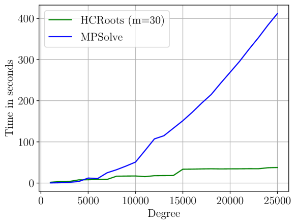
we can see in Figure 2, for random polynomial that are
known to be well-conditioned (see
Section 1.2.3), our solver HCRoots
called with a precision parameter is an order of
magnitude faster than MPSolve, which is very promising.
In our experiments, we focused on polynomials where the coefficients
are centered, Gaussian random variables with variance . In this case,
the solutions returned by our solver matched all the solutions returned by
MPSolve with an error less than , for polynomials up to
degree . Moreover, the linear
complexity of our algorithm, combined with the fact that we don’t need
to use multi-precision arithmetic, allowed us to solve polynomials of degree
25000 an order of magnitude faster than MPSolve. In
Figure 2, we show the timings to solve random
polynomials of degree with our solver, and MPSolve. Moreover,
it is easy to parallelize our algorithm, and improve furthermore its
practical efficiency.
2 Preliminaries
2.1 Notations
Given a polynomial or an analytic series , we will denote by and the derivative and the second derivative of . If is a polynomial, we will denote by , and the classical norm , and infinity on the vector of its coefficients. We will denote by the complex disk of radius centered at . Finally, for a polynomial and a root of , we let and is the absolute condition number of . It is also denoted and referred as the condition number of .
2.2 Fast elementary operations
We start with classical results on elementary operations, notably on the multiplication and the composition of polynomials.
Proposition 1 ([41, Theorem 2.2], [39, Proposition 3.2]).
Let and be two polynomials of degree with and less than , and an integer . It is possible to compute the polynomial such that in bit operations.
Using Fast Fourier transform algorithm, we can also evaluate in a quasi-linear time a polynomial on the roots of unity. Note that in this case, even if the required precision is smaller than , the algorithm is still quasi-linear in .
Proposition 2 ([41, §3], [39, Proposition 3.3]).
Let be a polynomial of degree , and with , and an integer . It is possible to compute the complex numbers such that in bit operations.
Finally, another classical result that we will use is the fast composition of polynomials.
Proposition 3 ([39, Theorem 2.2]).
Let and be two polynomials of degree with and where and . Let be a positive integer. It is possible to compute the polynomial of degree such that in bit operations.
Remark 5.
Ritzmann [39, Theorem 2.2] used the same bound for and . Our proposition is a direct consequence of Ritzmann’s theorem if we multiply in the input by , and the result by . This reduction can be done in bit operations.
2.3 Fast approximate multipoint evaluation
When we want to evaluate a polynomial on multiple points, it is possible to amortize the number of bit operations when the precision required is larger than the degree. In a recent work [45, §3.2], van der Hoeven showed that it can be done in . However, this bound is not optimal when is greater than . For the case , we recall here another state-of-the-art bound on the bit complexity for fast multipoint evaluation.
Proposition 4 ([45, Lemma 11], [30, Theorem 9]).
Let be a polynomial of degree , with , with , and let be complex points with absolute values bounded by . Then, computing such that for all is possible in bit operations.
Even though the bit complexity is quadratic in , this approach is near optimal when is greater than , since its complexity matches the size of the output in this case. We reuse notably this result to bound the complexity of Algorithm 2, since our approach reduces the problem of evaluating a polynomial of degree to the problem of evaluating several polynomials of degree with a precision greater than .
2.4 Condition number
Our root isolation algorithm has a bit complexity that depends on the condition number of the input polynomial. The absolute condition number is a measure of the displacement of its roots with respect to the displacement of its coefficients. More precisely, for a polynomial with a vector of coefficients , and a root of , there exists a neighborhood of , a neighborhood of and a differentiable function that maps to the unique zero in of the corresponding polynomial. Letting be the gradient of at , the condition number of at is the induced norm . If we consider the induced norm instead, we have .
Definition 3.
[8, §14.1.1] The standard local absolute condition number of polynomial of degree at a root is . Considering all the roots, we define the standard absolute condition number of as .
Remark 6.
The standard absolute condition number is obtained by considering the norm . If we consider the induced norm instead, we get the condition number , such that .
As shown in Remark 6, the bound depending on the logarithm of the condition number for the norm and the norm will be the same up to a factor logarithmic in . In the following, we will focus on the condition number induced by the norm .
For square-free polynomial with integer coefficients, the condition number is finite. The following proposition bounds the condition number for square-free polynomials with integer coefficients.
Proposition 5 ([32, last inequality]).
Given a square-free polynomial of degree with integer coefficients, let be a real such that . Then is in .
In particular, combined with Theorem 3, this proposition implies that for square-free polynomials, the bit-complexity of Algorithm 3 has the same worst-case bound as the state-of-the-art root-finding methods. We define also the relative condition number to represent the relative displacement of the roots, with respect to a relative displacement of the coefficients.
Definition 4 ([8, §14.1.1]).
The standard local relative condition number of a polynomial at a root is , and the standard relative condition number of is . Similarly, we define , and the associated relative condition number of is .
Remark 7.
An interesting property of the relative condition number at a nonzero root of is that it is equal to the relative condition number at the root of the polynomial . Moreover for the absolute condition number we have for outside the unit disk.
Proof of the remark.
By construction, the inverse function is a bijection between the non-zero roots of and the non-zero roots of . Computing the derivative of at a root we have . Thus . Finally, since by construction, we have . ∎
This number is a standard way to measure to stability of the roots with respect to independent perturbations of the coefficients. In Theorem 4, we provide a geometric criterion to bound from below this condition number.
2.5 Fast approximate factorization
Another important result on univariate polynomials is a bound on the bit complexity to approximate all its roots. In the complex, approximating the roots is equivalent to compute an approximate factorization. We recall the state-of-the-art bound on the bit complexity for this problem.
Proposition 6 ([37, Theorem 2.1.1]).
Let be a polynomial of degree with leading coefficient and all its roots in the unit disk, and a fixed real number. It is possible to compute complex numbers such that in bit operations.
Remark 8.
Proof of the remark.
Let . Then has all its roots in the unit disk and . Computing the approximate factorization of such that can be done in since . Then with the change of variable , we have . ∎
This theorem does not directly give a bound on the distances between the roots. Schönhage shows [42, §19] that in the worst case . This bound can be improved for well-conditioned roots. In our case, we will also need a bound on the distance between some pairs of roots of two polynomials that have different degrees. We will use Kantorovich theory for the bounds in these cases (Section 2.6 and 5.1).
Note that Remark 8 requires a bound on the modulus of the roots of the polynomial. For that, we will use the classical Fujiwara bound.
Proposition 7 ([18]).
Let be a polynomial of degree . Then the moduli of the roots of are lower or equal to
2.6 Certification of the roots
Several approaches in the literature guarantee that a neighborhood of a point contains a unique root of a given polynomial. We may cite notably Kantorovich criterion [12, §3.2], Smale’s alpha theorem [12, §3.3], Newton interval method [36, Theorem 5.1.7], Pellet’s test [33], Pellet’s test combined with Graeffe iteration [3, 27], Cauchy’s integral theorem [26, 25], and others [40], …A first crude bound from the literature to guarantee that a disk centered at a point contains a root of a polynomial is the following.
Proposition 8 ([22, Theorem 6.4e], [6, Theorem 9]).
Let be a polynomial of degree , and a complex point. Let . Then, for all , the disk contains a root of . In particular, the disk contains a root of .
With some additional conditions, Kantorovich criterion provides a smaller radius to guarantee that a disk contains a root .
Proposition 9 ([12, Theorem 88]).
Given a function of class , and a point such that , let , and . If , then has a root in the disk .
The previous propositions are useful to find a disk that contains a root of , but they don’t guarantee that the disk contains a unique root of . In order to prove that Algorithm 3 terminates and to bound its complexity, we use the lower bound from Kantorovich theory on the size of the basin of attraction of the roots of . More precisely, for each root , we bound the size of a disk containing where the Newton method always converges toward .
Proposition 10 ([12, Theorem 85]).
Given a function of class , and a root such that . If there exists such that , with , then is the unique root of in the disk . Moreover, for any , the Newton sequence defined by converges toward .
Remark 9.
If is a polynomial of degree , and , then a consequence of Proposition 10 is that the set of disks , for all roots of in the unit disk, are pairwise distinct.
For any complex point , we also prove the following lemma to have a criterion guaranteeing that a ball around is included in a basin of attraction of a root of .
Lemma 1.
Given a function of class and a point such that . Let and for all . If then, has a unique root in , and for all , the Newton sequence starting from converges to .
2.7 Geometric range searching
Our data structure can be seen as a piecewise polynomial approximation. As such, when doing multipoint evaluation, we will need to report the points that fall in a disk. This problem can be solved efficiently using classical range searching and point intersection searching algorithms.
Proposition 11 ([1, §5.2, Table 7]).
Given points in , it is possible to compute a data structure in operations such that for any disk , returning the list of points contained in can be done in operations, where is the number of points in .
Moreover, when we isolate the roots of a polynomial , we reduce the problem to isolate the roots in each disk of an -hyperbolic covering. Because those disks overlap, we need to remove redundant boxes. For that, we use fast rectangle-rectangle searching techniques.
Proposition 12 ([1, §3.6]).
Given rectangles in the plane, it is possible to compute a data structure in such that for any rectangle , returning the list of rectangle intersecting can be done in operations, where is the number of rectangles intersecting .
Note that in an -hyperbolic covering, each disk intersect at most other disks of the covering. Indeed the disks centered in the disk , it intersects at most other disks. For and a disk with a center between the circle of radius and a circle of radius , it intersects disks of the hyperbolic covering that have their centers in the same ring. Then it can intersects at most other disks coming from the inner adjacent ring, and other from the outer adjacent ring. Thus, in Algorithm 3, this will guarantee that each query will be done in (see Section 5.2).
3 Computation of the hyperbolic approximation
3.1 Properties
First, given an integer and a polynomial of degree , and a pair from the hyperbolic approximation , we give a bound on the coefficients of the polynomials . That gives also a bound on the polynomial , since is an approximation of the polynomial truncated to the degree .
Lemma 2.
Given a polynomial of degree and a integer , let be an affine transformation appearing in the hyperbolic approximation . Letting and , we have
Proof.
By construction, is of the form , with and two positive real numbers. Letting , and expanding the , we have . We now distinguish two cases. First if , then by construction of the sequences in Definition 1, we have . Thus . This proves the desired bound for both the cases where and the case where .
Then, if , then and , where . Then . Using the inequalities and we have . Moreover, , such that . This also proves the desired bound for both the cases where and the case where . ∎
We also give a bound on the number of disks appearing in the decomposition.
Lemma 3.
Given two integers and , let and let . Then the number of disks in the -hyperbolic covering is in . Moreover, the union of the disks contains the unit disk.
Proof.
First, remark that the total number of disks in a -covering is . Such that using Remark 1 we have , and . Thus the number of disks is in .
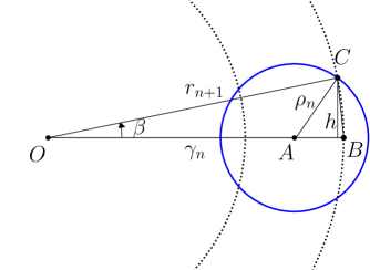
Then, we need to prove that for any ring , the union of the disks centered at with radius contains . For that, let be the disk and let be the segment intersection of with the half-line starting from and with angle . Then, let be the smallest angle such that is not included in . Then if the angle it implies that for all , the segment is included in a disk of the -hyperbolic covering.
Since , it is sufficient to prove that . Consider the triangle with , and (see Figure 3). Letting , remark that is the angle .
Let be the distance between the point and the line . By construction, . If we prove that the angles at vertex and vertex are each smaller than , then we can conclude that . Such that .
In order to prove that the angles at and are smaller than , remark that the triangle is isosceles, such that the angle is less than . Moreover, considering the triangle , the angle is larger than if . This inequality holds for since . Thus is less than . Since the angle of the triangle at the vertices and are less than , we can conclude that for all , is small enough to let the disks cover the unit disk.
∎
Finally, we give a bound on the bit size of the coefficients of the polynomials of an hyperbolic approximation, by bounding the size of the polynomials , leading also to a bound the its second derivative.
Lemma 4.
Given a polynomial of degree and an affine transform from an -hyperbolic approximation of , let . Letting , we have and for all , we have .
Proof.
Let be of the form . Let . Since and are positive numbers, we have . By construction, with . This implies that and thus . Then, we obtain the bound on the derivative and second derivative of by bounding the absolute value of the derivative and second derivative of each term . By construction, either or and .
In the former case, using binomial inequalities, we have such that . In the second case, with , we have , which implies .
∎
3.2 Proof of Theorem 1
We can now prove that Algorithm 1 returns an hyperbolic approximation of a polynomial with a complexity quasi-linear in the degree and the required precision.
Correctness.
First, for the correctness of the algorithm, we will prove that Algorithm 1 returns a list of pairs satisfying the constraints of Definition 2. First the affine transforms computed in Algorithm 1 send the unit disk to the disks described in Definition 1 of a hyperbolic covering. Then, the polynomials computed are approximation of the polynomials . We will show that the approximation satisfies the bound .
In part of Algorithm 1, we start by truncating to . The resulting polynomial satisfies . Let be of the form and let . Since and are positive numbers, we have . In the case where and , we have . Thus . Moreover, since . This implies that .
Then, the algorithm will evaluate on and , modulo and modulo . The advantage is that composition modulo can be done efficiently using Proposition 3 and evaluation modulo on can be reduced to Fast Fourier Transform and be done efficiently too using Proposition 2. The part up to can perform this computation with an error less than on each coefficients. More precisely, in the algorithm computes . Then in we have . Letting , the truncated polynomial associated to the disk of center and radius is . In step , for a fixed and a fixed between and , the coefficient of of , denoted by , is . Those coefficients can be computed efficiently using the fast Fourier transform algorithm. Such that using the notation of Algorithm 1 we finally have .
Finally, letting , we have by Lemma 2 that for all . Thus, we have .
Gathering the norm inequalities, we have as required:
Complexity.
The number of loop iterations in Algorithm 1 is in . Thus, it is sufficient to prove that each iteration can be performed in to achieve the complexity in Theorem 1. First, part can be done in operations. Then in part , we will use the state-of-the-art complexity bounds on the elementary operations recalled in Section 2.2.
First, in part and , we are reordering the coefficients, gathering together the coefficients of with the same value , which can be done in bit operations. Note that the polynomials computed in this part have a degree less than , with and , such that the degree of is in .
Then in part , we do multiplication of polynomials of degree in with an absolute error on the result in . Moreover, we have . Since , this implies . Using Proposition 1, each multiplication can be done in bit operations, and part requires bit operations.
Similarly, in part , since and , using proposition 3 on fast composition, we can compute with an error less than in . We also perform the multiplication by in this part within the same complexity. Overall, since the composition and the multiplication is done times, part can be done in operations.
Finally, in part , we use the Fast Fourier Transform algorithm to evaluate of degree on the roots of unity . If for an integer , the evaluation of on the points with an error less than can be done in using Proposition 2. Thus the bit complexity for part is in . To bound , remark that . Let be the polynomial where we replaced the coefficients by their absolute value. In this case . Moreover . In turn , and , such that . Finally, . Thus part can be computed in bit operations.
4 Multipoint evaluation
A direct application of our data structure is the fast evaluation of polynomials. The main idea is to approximate the input polynomial with a piecewise polynomial, where each polynomial has a degree with the same order of magnitude as the required precision. Then we can use state-of-the-art multipoint evaluation technique on each .
Proof of Theorem 2.
The correction of Algorithm 2 is ensured by the fact that for all in a disk , letting , we have . If we compute the evaluation of with an error less than , the result will have an error less than , using the bound on given in Lemma 4. So finally we have .
First the data structure can be computed in
using Proposition 11, and the hyperbolic approximation
in using Theorem 1. Then in the
loop, the algorithm queries the points in
using Proposition 11.
Let be the degree of , and . We can evaluate on
points using times the fast multipoint evaluation method in
Proposition 4. For an absolute error less than
, this can be done in bit
operations. Note that , such that the total
complexity in an iteration of the for loop is in . Note also that the sum of the is .
If is the number of discs in the hyperbolic approximation, after adding the complexity of all the
main loop iterations, Algorithm 2 requires
. By Lemma 3, is in
, such that the total complexity of
Algorithm 2 is in .
∎
5 Root isolation
5.1 Properties of the approximate roots
We start by describing the properties satisfied by the roots of the truncated polynomials coming from an -hyperbolic approximations. In particular, we show how to perturb them such that all their roots are contained in a small enough disks.
Lemma 5.
Let be two positive integers. Let be a polynomial of degree and be a constant such that and for . Then for the roots of the polynomial are in the disk .
Proof.
Using the Fujiwara bound on the modulus of the roots of a polynomial (Proposition 7) on the polynomial , we have for , and for we have . Finally for , . ∎
Then we will use a technical lemma that gives a bound on the derivative of the difference of an analytic function and a polynomial, given bounds on their coefficients and the difference of their coefficients.
Lemma 6.
Let be an analytic series with radius of convergence greater than . Let be a polynomial of degree and be a positive real number such that: and for all . Then, for all in the unit disk we have
Proof.
Using the bounds on the coefficients of and , we have . The sum can be bounded using the function defined for a real in . We have and , such that . Also we have . This leads to ∎
For an analytic function , this allows us to prove that if a polynomial is a good enough approximation of , each root of in the unit disk is near a root of .
Lemma 7.
Let be an analytic series with radius of convergence greater than . Let be a polynomial of degree and be a positive real number such that: and for all . Let be a root of in the unit disk such that and let .
If , then has a root in .
Remark 10.
If , the inequality holds as soon as .
Proof.
Using Proposition 8, if , then has a root in the disk . Since is in the unit disk, . For the derivative, we have . The difference between the derivative of and can be bounded using Lemma 6 by . Since , this implies , which allows us to conclude.
∎
Finally, to prove that Algorithm 3 terminates, we will need the following lemma that guarantees that the criterion of Lemma 1 will be satisfied for a small enough approximation.
Lemma 8.
Let be an analytic series with radius of convergence greater than and be a root of in the unit disk such that . Let and be positive real greater than for all in the disk . Then, for any positive real and all :
Proof.
Using Taylor expansion at , we have , and thus . Similarly, . Factoring out in the numerator, and in the denominator, this leads to . Since , the numerator is less than and the denominator is greater than , such that .
∎
5.2 Proof of Theorem 3
We can now prove the main theorem bounding the bit complexity of Algorithm 3. We split our proof in three part. First the correctness, then the termination and finally a bound on the complexity of Algorithm 3.
Correctness.
First, the correctness of Algorithm 3 follows from Lemma 1. Indeed, using Lemma 4 and Lemma 6, each disk added to satisfies the condition of Lemma 1 and contains a unique root of . Then, if the algorithm terminates, it returns a list of pairwise distinct disks, containing a root of each, such that the result is correct.
Termination.
For the termination of Algorithm 3, we fix and we will use Lemma 7 and 8 to show that for sufficiently large, Algorithm 3 terminates. First, using Lemma 7 to bound the distance between a root of and the closest root of , we need a bound and a bound on the condition number of . The first bound comes from . Using Lemma 4, we have , such that . Moreover, and for . This leads to . For the bound on the condition number, since is of the form , this implies that for all in the unit disk , such that . Letting , we have that for each root of , if , Lemma 7 implies that there exists a root of in the disk , where .
We will now use this property with Lemma 8 to show that the criterion computed on line 3 of Algorithm 3 will eventually be satisfied. Using the notations of Algorithm 3, we show that the criterion will be satisfied for all roots of for large enough. Let . Using the bound on given by Definition 2 and the bound on given by Lemma 6, we have . Moreover is in the disk , with . From Lemma 8, we can conclude that is smaller than for , that is for , which holds as soon as . Note that for , is smaller than , such that for all and the algorithm terminates after iterations of the main loop.
Complexity bound.
First, at each iteration of the main while loop, computing the
-hyperbolic approximation costs bit operations.
Then for a fixed , the approximate factorization
is called times on polynomials of degree , with bit operations for
each call, using Proposition 6. With Remark 8, this bound holds for
polynomial that have all their roots of modulus less than .
By Lemma 2, the coefficients of the polynomial
satisfy the condition of Lemma 5 and we conclude
that all its
roots of are included in .
Thus the approximate factorization can be computed within .
Thus, for all cases, the total cost for the approximate factorization
in an iteration of the while loop is in bit
operations. After that, for each , we need to evaluate and
up to a precision in . This can be done
using state-of-the-art fast approximate multipoint evaluation in
for all the approximate roots of
using Proposition 4. This amounts to a total of
bit operations for the steps
3 to 3. If , then the
factorization is called a constant number of times on polynomials of
degree , for a total cost in bit operations, and
all the multipoint evaluations will cost a total of bit operations. Finally, removing
duplicate solutions can be done in operations.
Indeed, by construction, given a box of in a disk of the
-hyperbolic covering, the number of times that it
appears in is bounded by the maximal number of disks of the -hyperbolic
covering that intersects , that is (see
Section 2.7). Thus, using
Proposition 12, this ensures that each query to
detect a duplicate will cost at most operations,
and removing all the duplicates will cost at most
bit operations. In total, the costs is per iteration of the
while loop. Since is doubled at each iteration, the cost is
the same as the cost of the last iteration, that is in bit operations.
6 Lower bound on the condition number
The lower bound on the condition number is a consequence of Lemma 7, that gives a bound on the distance between the roots of two polynomials with close enough coefficients, applied on the polynomials from the adapted hyperbolic approximation. Essentially, the idea is that for any greater or equal to function of and for any pair of an -hyperbolic approximation of , the number of roots of is greater than the number of roots of in the disk . In particular, this property allows us to deduce a lower bound on depending on the number of roots of in the disk .
Proof of Theorem 4.
Let be a disk where the number of solutions of is maximal. Without restriction of generality, using Remark 3, we can assume that the absolute value of the center of is less than . Up to a change of variable , where is a complex number of modulus , we can assume that the center of is a positive real number. Letting , we can see easily that is included in a disk of the -hyperbolic covering of the unit disk. Let and let be the polynomial of degree obtained by truncating at order . By Lemma 2, the coefficients of for degree are less than . Using the bounds in Lemma 4, we have for all in the unit disk . Moreover , and , such that . Let , and . We can now prove by contradiction that the number of roots of exceeds its degree if . Indeed in this case, by Lemma 7, for each root of , the polynomial has a root in . Moreover, using Remark 9, for all the roots of in the unit disk, the disks are pairwise distinct, such that has at least roots. Thus, to avoid this contradiction, we thus have . That is, we must have either or . Equivalently, this amounts to . For , this implies . Finally, for each root of with we have , which allows us to conclude. ∎
Acknowledgement
The author thanks the anonymous reviewers for their thoughtful comments on this work and on a previous related work.
Appendix A Source code
For the reproducibility of our experiments, and to demonstrate the
conciseness of our implementation, we report here the full source code of our root
solver
HCRoots, along with an implementation of the multipoint evaluation algorithm
(hceval.py), both available on a public gitlab server [35].
References
- [1] Pankaj K Agarwal and Jeff Erickson. Geometric range searching and its relatives. In B. Chazelle, J. E. Goodman, and R. Pollack, editors, Advances in discrete and computational geometry, volume 223 of Contemporary Mathematics, pages 1 – 56. American Mathematical Society, Providence, RI, 1999.
- [2] Alfred V. Aho and John E. Hopcroft. The Design and Analysis of Computer Algorithms. Addison-Wesley Longman Publishing Co., Inc., USA, 1st edition, 1974.
- [3] Ruben Becker, Michael Sagraloff, Vikram Sharma, and Chee Yap. A near-optimal subdivision algorithm for complex root isolation based on the pellet test and newton iteration. Journal of Symbolic Computation, 86:51 – 96, 2018.
- [4] Carlos Beltrán and Luis Miguel Pardo. Fast linear homotopy to find approximate zeros of polynomial systems. Foundations of Computational Mathematics, 11(1):95–129, Feb 2011.
- [5] Todor Bilarev, Magnus Aspenberg, and Dierk Schleicher. On the speed of convergence of newton’s method for complex polynomials. Mathematics of Computation, 85(298):693–705, 2016.
- [6] Dario A. Bini and Giuseppe Fiorentino. Design, analysis, and implementation of a multiprecision polynomial rootfinder. Numerical Algorithms, 23(2):127–173, Jun 2000.
- [7] Dario A. Bini and Leonardo Robol. Solving secular and polynomial equations: A multiprecision algorithm. Journal of Computational and Applied Mathematics, 272:276–292, 2014.
- [8] Peter Bürgisser and Felipe Cucker. Condition: The Geometry of Numerical Algorithms. Springer Berlin Heidelberg, Berlin, Heidelberg, 2013.
- [9] Peter Bürgisser, Felipe Cucker, and Elisa Rocha Cardozo. On the condition of the zeros of characteristic polynomials. Journal of Complexity, 42:72–84, 2017.
- [10] Felipe Cucker, Teresa Krick, Gregorio Malajovich, and Mario Wschebor. A numerical algorithm for zero counting, i: Complexity and accuracy. Journal of Complexity, 24(5):582–605, 2008.
- [11] Felipe Cucker and Steve Smale. Complexity estimates depending on condition and round-off error. J. ACM, 46(1):113–184, January 1999.
- [12] Jean-Pierre Dedieu. Points fixes, zéros et la méthode de Newton. Mathématiques et Applications. Springer Berlin Heidelberg, Berlin, Heidelberg, 2006.
- [13] Yen Do, Hoi Nguyen, and Van Vu. Real roots of random polynomials: expectation and repulsion. Proceedings of the London Mathematical Society, 111(6):1231–1260, 2015.
- [14] Alan Edelman and Eric Kostlan. How many zeros of a random polynomial are real? Bulletin of the American Mathematical Society, 32(1):1–37, 1995.
- [15] Louis W. Ehrlich. A modified newton method for polynomials. Commun. ACM, 10(2):107–108, February 1967.
- [16] Ioannis Z. Emiris, Victor Y. Pan, and Elias Tsigaridas. Algebraic algorithms. Chapter 10 of Computing Handbook , Volume I: Computer Science and Software Engineering (Allen B. Tucker, Teo Gonzales, and Jorge L. Diaz-Herrera, editors), 2014.
- [17] Charles M. Fiduccia. Polynomial evaluation via the division algorithm the fast fourier transform revisited. In Proceedings of the Fourth Annual ACM Symposium on Theory of Computing, STOC ’72, page 88–93, New York, NY, USA, 1972. Association for Computing Machinery.
- [18] Matsusaburô Fujiwara. Über die obere schranke des absoluten betrages der wurzeln einer algebraischen gleichung. Tohoku Mathematical Journal, First Series, 10:167–171, 1916.
- [19] Jean Ginibre. Statistical ensembles of complex, quaternion, and real matrices. Journal of Mathematical Physics, 6(3):440–449, 1965.
- [20] Xavier Gourdon. Algorithmique du theoreme fondamental de l’algebre. Research Report RR-1852, INRIA, 1993. HAL: https://hal.inria.fr/inria-00074820.
- [21] Charles R. Harris, K. Jarrod Millman, Stéfan J. van der Walt, et al. Array programming with NumPy. Nature, 585(7825):357–362, September 2020.
- [22] Peter Henrici. Applied and computational complex analysis, Vol. 1. Wiley, New York, 1974.
- [23] J. Ben Hough, Majunath Krishnapur, Yuval Peres, and Bálint Virág. Determinantal processes and independence. Probability Surveys, 3:206–229 (electronic), 2006. 00000.
- [24] John Hubbard, Dierk Schleicher, and Scott Sutherland. How to find all roots of complex polynomials by newton’s method. Inventiones mathematicae, 146(1):1–33, Oct 2001.
- [25] Rémi Imbach and Victor Y. Pan. New practical advances in polynomial root clustering. In Daniel Slamanig, Elias Tsigaridas, and Zafeirakis Zafeirakopoulos, editors, Mathematical Aspects of Computer and Information Sciences, pages 122–137, Cham, 2020. Springer International Publishing.
- [26] Rémi Imbach and Victor Y. Pan. New progress in univariate polynomial root finding. In Proceedings of the 45th International Symposium on Symbolic and Algebraic Computation, ISSAC ’20, page 249–256, New York, NY, USA, 2020. Association for Computing Machinery.
- [27] Rémi Imbach, Victor Y. Pan, and Chee Yap. Implementation of a near-optimal complex root clustering algorithm. In James H. Davenport, Manuel Kauers, George Labahn, and Josef Urban, editors, Mathematical Software – ICMS 2018, pages 235–244, Cham, 2018. Springer International Publishing.
- [28] Zakhar Kabluchko and Dmitry Zaporozhets. Asymptotic distribution of complex zeros of random analytic functions. The Annals of Probability, 42(4):1374 – 1395, 2014.
- [29] R. Baker Kearfott. Rigorous global search: continuous problems. Nonconvex optimization and its applications. Kluwer Academic Publishers, Dordrecht, Boston, 1996.
- [30] Alexander Kobel and Michael Sagraloff. Fast approximate polynomial multipoint evaluation and applications, 2016. arXiv:https://arxiv.org/abs/1304.8069v2 [cs.NA].
- [31] Pierre Lairez. A deterministic algorithm to compute approximate roots of polynomial systems in polynomial average time. Foundations of Computational Mathematics, 17(5):1265–1292, Oct 2017.
- [32] Kurt Mahler. An inequality for the discriminant of a polynomial. Michigan Mathematical Journal, 11(3):257 – 262, 1964.
- [33] Kurt Mehlhorn, Michael Sagraloff, and Pengming Wang. From approximate factorization to root isolation with application to cylindrical algebraic decomposition. Journal of Symbolic Computation, 66:34–69, 2015.
- [34] Ramon E. Moore, R. Baker Kearfott, and Michael J. Cloud. Introduction to interval analysis. Siam, 2009.
- [35] Guillaume Moroz. HCRoots: Hyperbolic Complex Root solver. https://gitlab.inria.fr/gmoro/hcroots, 2021.
- [36] Arnold Neumaier. Interval methods for systems of equations. Cambridge University Press, 1990.
- [37] Victor Y. Pan. Univariate polynomials: Nearly optimal algorithms for numerical factorization and root-finding. Journal of Symbolic Computation, 33(5):701–733, 2002.
- [38] Yuval Peres and Bálint Virág. Zeros of the i.i.d. Gaussian power series: a conformally invariant determinantal process. Acta Mathematica, 194(1):1 – 35, 2005.
- [39] Peter Ritzmann. A fast numerical algorithm for the composition of power series with complex coefficients. Theoretical Computer Science, 44:1–16, 1986.
- [40] Siegfried M. Rump. Ten methods to bound multiple roots of polynomials. Journal of Computational and Applied Mathematics, 156(2):403 – 432, 2003.
- [41] Arnold Schönhage. Asymptotically fast algorithms for the numerical multiplication and division of polynomials with complex coefficients. In Jacques Calmet, editor, Computer Algebra, pages 3–15, Berlin, Heidelberg, 1982. Springer Berlin Heidelberg.
- [42] Arnold Schönhage. The fundamental theorem of algebra in terms of computational complexity. Technical report, Departement of Mathematics, University of Tübingen, Germany, 1982. updated 2004.
- [43] Steve Smale. The fundamental theorem of algebra and complexity theory. Bull. Amer. Math. Soc. (N.S.), 4(1):1–36, 01 1981.
- [44] Mikhail Sodin and Boris Tsirelson. Random complex zeroes, i. asymptotic normality. Israel Journal of Mathematics, 144(1):125–149, Mar 2004.
- [45] Joris van der Hoeven. Fast composition of numeric power series. Technical Report 2008-09, Université Paris-Sud, Orsay, France, 2008.
- [46] Joachim von zur Gathen and Jürgen Gerhard. Modern Computer Algebra. Cambridge University Press, Cambridge, U.K., 3 edition, 2013.
- [47] Rephael Wenger. Isosurfaces: geometry, topology, and algorithms. CRC Press, 2013.
- [48] James H. Wilkinson. The evaluation of the zeros of ill-conditioned polynomials. part ii. Numerische Mathematik, 1(1):167–180, Dec 1959.
- [49] James H. Wilkinson. Rounding errors in algebraic processes. Englewood Cliffs, N.J: Prentice-Hall, 1964.