Lattice gauge theories in the presence of a linear gauge-symmetry breaking

Abstract

We study the effects of gauge-symmetry breaking (GSB) perturbations in three-dimensional lattice gauge theories with scalar fields. We study this issue at transitions in which gauge correlations are not critical and the gauge symmetry only selects the gauge-invariant scalar degrees of freedom that become critical. A paradigmatic model in which this behavior is realized is the lattice CP¹ model or, more generally, the lattice Abelian-Higgs model with two-component complex scalar fields and compact gauge fields. We consider this model in the presence of a linear GSB perturbation. The gauge symmetry turns out to be quite robust with respect to the GSB perturbation: the continuum limit is gauge-invariant also in the presence of a finite small GSB term. We also determine the phase diagram of the model. It has one disordered phase and two phases that are tensor and vector ordered, respectively. They are separated by continuous transition lines, which belong to the O(3), O(4), and O(2) vector universality classes, and which meet at a multicritical point. We remark that the behavior at the CP¹ gauge-symmetric critical point substantially differs from that at transitions in which gauge correlations become critical, for instance at transitions in the noncompact lattice Abelian-Higgs model that are controlled by the charged fixed point: in this case the behavior is extremely sensitive to GSB perturbations.

I Introduction

Gauge symmetries have been crucial in the development of theoretical models of fundamental interactions Wilson-74 ; Weinberg-book ; ZJ-book . They also play a relevant role in statistical and condensed-matter physics  Wen-book ; Anderson-15 ; GASVW-18 ; Sachdev-19 ; SSST-19 ; GSF-19 ; Wetterich-17 ; FNN-80 ; INT-80 . For instance, it has been suggested that they may effectively emerge as low-energy effective symmetries of many-body systems. However, because of the presence of microscopic gauge-symmetry violations, it is crucial to understand the role of the gauge-symmetry breaking (GSB) perturbations. One would like to understand whether these perturbations do not change the low-energy dynamics—in this case the gauge-symmetric theory would describe the asymptotic dynamics even in the presence of some (possibly small) violations—or whether even small perturbations can destabilize the emergent gauge model— consequently, a gauge-invariant dynamics would be observed only if an appropriate tuning of the model parameters is performed. This issue is also crucial in the context of analog quantum simulations, for example, when controllable atomic systems are engineered to effectively reproduce the dynamics of gauge-symmetric theoretical models, with the purpose of obtaining physical information from the experimental study of their quantum dynamics in laboratory. Several proposals of artificial gauge-symmetry realizations have been reported, see, e.g., the review articles ZCR-15 ; Banuls-etal-20 ; BC-20 and references therein, in which the gauge symmetry is expected to effectively emerge in the low-energy dynamics.

Previous studies of the critical behavior (or continuum limit) of three-dimensional (3D) lattice gauge theories with scalar matter have shown the emergence of two different scenarios. One possibility is that scalar-matter and gauge-field correlations are both critical at the transition point. This behavior is related to the existence of a charged fixed point (FP) in the renormalization-group (RG) flow of the corresponding continuum gauge field theory ZJ-book . This is realized in some of the transitions observed in the 3D lattice Abelian-Higgs (AH) model with noncompact gauge fields BPV-21 . Alternatively, it is possible that only scalar-matter correlations are critical at the transition. The gauge variables do not display long-range critical correlations, although their presence is crucial to identify the gauge-invariant scalar-matter degrees of freedom that develop the critical behavior. This typically occurs in lattice AH models with compact gauge variables.

In Ref. BPV-21-gsb we studied GSB perturbations in the 3D lattice AH model with noncompact gauge field, at transitions controlled by the charged FP of the RG flow of 3D electrodynamics with multicomponent charged scalar fields HLM-74 ; FH-96 ; IZMHS-19 ; ZJ-book ; MZ-03 (also called AH field theory). In that case a photon-mass GSB term, however small, gives rise to a drastic departure from the gauge-invariant continuum limit of the statistical lattice gauge theory, driving the system towards a different critical behavior (continuum limit). This is due to the fact that a photon-mass term qualitatively changes the phase diagram of the noncompact lattice AH theory BPV-21 . The Coulomb phase is no longer present and therefore, the nature of the transition to the Higgs phase, previously controlled by the charged fixed point, varies. One ends up with a new critical behavior with noncritical gauge fields.

At transitions where gauge fields are not critical, the role of gauge symmetries is more subtle, but still crucial to determine the continuum limit. Even if gauge correlations are not critical, gauge fields prevent non-gauge invariant correlators from acquiring nonvanishing vacuum expectation values and therefore, from developing long-range order. Therefore, gauge symmetries effectively reduce the number of degrees of freedom of the matter-field critical modes. The lattice CP^N-1 model PV-19-CP ; TIM-05 ; TIM-06 or, more generally, the lattice AH model with compact gauge fields PV-19-AH3d , where an $N$-component complex scalar field is gauge-invariantly coupled to a compact U(1) gauge field associated with the links of the lattice, have transitions of this type. In these models the role of the U(1) gauge symmetry is that of hindering some scalar degrees of freedom, i.e., those related to a local phase, from becoming critical. As a consequence, the critical behavior or continuum limit is driven by the condensation of a gauge-invariant tensor scalar operator, and the corresponding continuum field theory is associated with a Landau-Ginzburg-Wilson (LGW) field theory with a tensor field, but without gauge fields. For $N=2$, the LGW approach predicts that the continuum limit of the CP¹ model (or of the $N=2$ lattice compact AH model) is equivalently described by the LGW field theory for a three-component real vector field with O(3) global symmetry.

In this paper we investigate the effects of perturbations breaking the gauge symmetry when gauge-field correlations are not critical and the gauge symmetry acts only to prevent some of the matter degrees of freedom from becoming critical. For this purpose we consider a lattice AH model with compact gauge fields, focusing on the case of two scalar components. We consider the most natural and simplest GSB term, adding to the Hamiltonian (or action, in the high-energy physics terminology) a term that is linear in the gauge link variable. This GSB term is similar to the photon mass term considered in noncompact lattice AH models, and indeed it is equivalent to it in the limit of small noncompact field $A_{{\bm{x}},\mu}$, as can be immediately seen by expanding the exponential relation between the compact and noncompact gauge fields, i.e., $\lambda_{{\bm{x}},\mu}=\exp(iA_{{\bm{x}},\mu})$. At variance with what was obtained in Ref. BPV-21-gsb , where we considered GSB perturbations at transitions controlled by charged FPs, in the present case the linear GSB perturbation does not change the continuum limit, at least for a sufficiently small finite strength of the perturbation.

In Fig. 1 we anticipate a sketch of the phase diagram of the lattice CP¹ model in the presence of a GSB term whose strength is controlled by the parameter $w$. It presents three different phases: a high-temperature (small $J$) disordered phase, and two low-temperature (large $J$) phases with different orderings. When the GSB perturbation is small, the low-temperature phase is qualitatively analogous to that of the gauge-invariant model, i.e., it is characterized by the condensation of a bilinear tensor scalar operator. In the RG language, the GSB perturbation turns out to be irrelevant at the FP of the gauge-invariant theory. On the other hand, when the GSB parameter $w$ is sufficiently large, there is a second ordered phase characterized by the condensation of the vector scalar field. These phases are separated by three different transition lines, meeting at a multicritical point. Along the disordered-tensor (DT) transition line we observe the same critical behavior as in the CP¹ model: the tensor degrees of freedom behave as in the O(3) vector model. The GSB term is irrelevant and the continuum limit of the model with a finite GSB breaking is the same as that of the gauge-invariant model. Along the DV line, we observe instead a different continuum limit: vector and tensor degrees of freedom behave as in the O(4) model. Finally, on the TV line we observe an O(2) vector critical behavior.

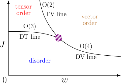
Figure 1: Sketch of the phase diagram of the lattice CP¹ model in the presence of the GSB term $H_{b}=-w\sum_{{\bm{x}},\mu}{\rm Re}\,\lambda_{{\bm{x}},\mu}$. This is a particular case of the lattice AH model with two-component scalar matter and compact gauge variables for $\gamma=0$. The phase diagram is characterized by three different phases: a disordered phase (small $J$), a tensor-ordered phase where the tensor operator $Q$ condenses (large $J$ and small $w$), and a vector-ordered phase where the vector field ${\bm{z}}_{\bm{x}}$ condenses (large $J$ and $w$). These phases are separated by the DT, DV, and TV transition lines, where CP¹/O(3), O(4) vector, and O(2) vector critical behavior is observed.

The paper is organized as follows. In Sec. II we define the lattice AH model with compact gauge variables and the linear GSB perturbation. In Sec. III we define the observables that we consider in the numerical study and review the main properties of the finite-size scaling (FSS) analyses employed. In Sec. IV we discuss some limiting cases where the thermodynamic behavior is known and propose a possible phase diagram for the model. In Sec. V we discuss our numerical results for $N=2$, which support the conjectured phase diagram. Finally, in Sec. VI we summarize and draw our conclusions. In the Appendix we report some universal curves in the O($N$) vector model, that allow us to identify the universality class of the different transitions.

II The model

II.1 The lattice Abelian-Higgs model with compact gauge variables

A compact lattice formulation of the three-dimensional AH model is obtained by associating complex $N$-component unit vectors ${\bm{z}}_{\bm{x}}$ with the sites ${\bm{x}}$ of a cubic lattice, and U(1) variables $\lambda_{{\bm{x}},\mu}$ with each link connecting the site ${\bm{x}}$ with the site ${\bm{x}}+\hat{\mu}$ (where $\hat{\mu}=\hat{1},\hat{2},\ldots$ are unit vectors along the positive lattice directions). The partition function of the system reads

$$Z=\sum_{\{{\bm{z}},\lambda\}}e^{-H_{\rm AH}({\bm{z}},\lambda)}\,,$$ (1)

$$H_{\rm AH}({\bm{z}},\lambda)=H_{z}({\bm{z}},\lambda)+H_{\lambda}(\lambda)\,.$$ (2)

We define

$$H_{z}=-J\,N\sum_{{\bm{x}},\mu}2\,{\rm Re}\,\lambda_{{\bm{x}},\mu}\,\bar{\bm{z}}_{\bm{x}}\cdot{\bm{z}}_{{\bm{x}}+\hat{\mu}}\,,$$ (3)

where the sum runs over all lattice links, and

$$H_{\lambda}=-\gamma\sum_{{\bm{x}},\mu>\nu}2\,{\rm Re}\,\Pi_{{\bm{x}},{\mu}\nu}\,,$$ (4)

where

$$\Pi_{{\bm{x}},{\mu}\nu}=\lambda_{{\bm{x}},{\mu}}\,\lambda_{{\bm{x}}+\hat{\mu},{\nu}}\,\bar{\lambda}_{{\bm{x}}+\hat{\nu},{\mu}}\,\bar{\lambda}_{{\bm{x}},{\nu}}\,,$$ (5)

and the sum runs over all plaquettes of the cubic lattice. The AH Hamiltonian is invariant under the global SU($N$) transformations

$$z_{\bm{x}}\to Uz_{\bm{x}}\,,\qquad U\in\mathrm{SU}(N)\,,$$ (6)

and the local U(1) gauge transformations

$$z_{\bm{x}}\to e^{i\theta_{\bm{x}}}z_{\bm{x}}\,,\quad\lambda_{{\bm{x}},\mu}\to e^{i\theta_{\bm{x}}}\lambda_{{\bm{x}},\mu}e^{-i\theta_{{\bm{x}}+\hat{\mu}}}\,,$$ (7)

where $\theta_{\bm{x}}$ is an arbitrary space-dependent real function. The parameter $\gamma\geq 0$ plays the role of inverse gauge coupling.

For $\gamma=0$, the model is a particular lattice formulation of the 3D CP^N-1 model, which is quadratic in the scalar-field variables and linear in the gauge variables. We can obtain a lattice formulation without explicit gauge fields by integrating out the link variables. We obtain

$$Z=\sum_{\{{\bm{z}},\lambda\}}e^{-H_{z}({\bm{z}},\lambda)}=\sum_{\{{\bm{z}}\}}\prod_{{\bm{x}},\mu}I_{0}\left(2JN|\bar{\bm{z}}_{\bm{x}}\cdot{\bm{z}}_{{\bm{x}}+\hat{\mu}}|\right)\,,$$ (8)

where $I_{0}(x)$ is a modified Bessel function. The corresponding effective Hamiltonian is

$$H_{{\rm eff}}=-\sum_{{\bm{x}},\mu}\ln I_{0}\left(2JN|\bar{\bm{z}}_{\bm{x}}\cdot{\bm{z}}_{{\bm{x}}+\hat{\mu}}|\right)\,,$$ (9)

which is invariant under the gauge transformations (7) even in the absence of gauge fields. For $J$ small, since $I_{0}(x)=1+x^{2}/4+O(x^{4})$, the Hamiltonian $H_{{\rm eff}}$ simplifies to

$$H_{CP}=-J^{2}N^{2}\sum_{{\bm{x}},\mu}|\bar{\bm{z}}_{\bm{x}}\cdot{\bm{z}}_{{\bm{x}}+\hat{\mu}}|^{2},$$ (10)

which represents another equivalent formulation of the CP^N-1 model.

The compact AH model presents two phases when varying $J$ and $\gamma$ PV-19-AH3d , separated by a transition line, whose nature does not depend on the gauge parameter $\gamma$. The appropriate order parameter is the bilinear gauge-invariant operator

$$Q_{{\bm{x}}}^{ab}=\bar{z}_{\bm{x}}^{a}z_{\bm{x}}^{b}-{1\over N}\delta^{ab}\,,$$ (11)

which is a hermitian and traceless $N\times N$ matrix. It transforms as $Q_{{\bm{x}}}\to{U}^{\dagger}Q_{{\bm{x}}}\,{U}$ under the global SU($N$) transformations. Its condensation signals the spontaneous breaking of the global SU($N$) symmetry.

II.2 Linear breaking of the U(1) gauge symmery

In the following we investigate the effects of perturbations breaking gauge invariance. In particular, we consider the simplest gauge-breaking perturbation that is linear in the $\lambda$ variables. We consider the extendend Hamiltonian

$$H_{e}({\bm{z}},\lambda)=H_{\rm AH}({\bm{z}},\lambda)+H_{b}(\lambda)\,,$$ (12)

where

$$H_{b}=-w\sum_{{\bm{x}},\mu}{\rm Re}\,\lambda_{{\bm{x}},\mu}\,.$$ (13)

Note that, if we perform the change of variables

$${\bm{z}}_{\bm{x}}\to(-1)^{x_{1}+x_{2}+x_{3}}{\bm{z}}_{\bm{x}}\ ,\quad\lambda_{{\bm{x}},\mu}\to-\lambda_{{\bm{x}},\mu}\,,$$ (14)

we reobtain the action (12), with $w$ replaced by $-w$. Thus, the phase diagram is independent of the sign of $w$ (but, for $w<0$, the relevant vector order parameters would be staggered quantities). Thus, in the following we only consider the case $w\geq 0$.

When $\gamma=0$, one can straightforwardly integrate out the link variables $\lambda$, obtaining

$$Z = \sum_{\{{\bm{z}},\lambda\}}e^{-H_{z}({\bm{z}},\lambda)-H_{b}(\lambda)}$$ (15)

$$= \sum_{\{{\bm{z}}\}}\prod_{{\bm{x}},\mu}I_{0}\left(2JN|\hat{w}+\bar{{\bm{z}}}_{\bm{x}}\cdot{\bm{z}}_{{\bm{x}}+\hat{\mu}}|\right),$$

where $\hat{w}=w/(2JN)$. The corresponding effective Hamiltonian reads

$$H_{{\rm eff}}=-\sum_{{\bm{x}},\mu}\ln I_{0}\left(2JN|\hat{w}+\bar{\bm{z}}_{\bm{x}}\cdot{\bm{z}}_{{\bm{x}}+\hat{\mu}}|\right)\,.$$ (16)

The Bessel function should be irrelevant for the critical behavior. Since, the argument of the Bessel function can be equivalently written as

$$|\hat{w}+\bar{\bm{z}}_{\bm{x}}\cdot{\bm{z}}_{{\bm{x}}+\hat{\mu}}|^{2}=\hat{w}^{2}+2\hat{w}\,\hbox{Re}\,(\bar{\bm{z}}_{\bm{x}}\cdot{\bm{z}}_{{\bm{x}}+\hat{\mu}})+|\bar{\bm{z}}_{\bm{x}}\cdot{\bm{z}}_{{\bm{x}}+\hat{\mu}}|^{2},$$ (17)

we expect that, for infinite gauge coupling, the model has the same critical behavior as a model with Hamiltonian

$$\widetilde{H}_{{\rm eff}}=-J^{2}N^{2}\sum_{{\bm{x}},\mu}\Big{[}|\bar{\bm{z}}_{\bm{x}}\cdot{\bm{z}}_{{\bm{x}}+\hat{\mu}}|^{2}+2\hat{w}\,{\rm Re}\,\bar{\bm{z}}_{\bm{x}}\cdot{\bm{z}}_{{\bm{x}}+\hat{\mu}}\Big{]}\,.$$ (18)

Such a Hamiltonian is the sum of a U($N$) invariant CP^N-1 model and an O($2N$) invariant vector model, which represents now the gauge-breaking perturbation. Thus, the introduction of the linear gauge-breaking term (13) is equivalent to the addition of a ferromagnetic vector interaction ${\rm Re}(\bar{\bm{z}}_{\bm{x}}\cdot{\bm{z}}_{{\bm{x}}+\hat{\mu}})$ among the vector fields. Although this has been shown for $\gamma=0$, we expect this equivalence to hold at criticality for any positive finite $\gamma$.

We would like now to show that, at transitions where the vector fields show a critical behavior, one observes an enlarged O($2N$) symmetry. For this purpose, note that the CP^N-1 interaction in Eq. (18) can be rewritten as

$$|\bar{\bm{z}}_{\bm{x}}\cdot{\bm{z}}_{{\bm{x}}+\hat{\mu}}|^{2}=({\rm Re}\,\bar{\bm{z}}_{\bm{x}}\cdot{\bm{z}}_{{\bm{x}}+\hat{\mu}})^{2}+({\rm Im}\,\bar{\bm{z}}_{\bm{x}}\cdot\Delta_{\mu}{\bm{z}}_{\bm{x}})^{2},$$ (19)

where $\Delta_{\mu}{\bm{z}}_{\bm{x}}\equiv{\bm{z}}_{{\bm{x}}+\hat{\mu}}-{\bm{z}}_{\bm{x}}$, and we used the fact that $\bar{\bm{z}}_{x}\cdot{\bm{z}}_{x}=1$. The first term represents an additional O($2N$) invariant vector ferromagnetic interaction, while the second one is only invariant under U($N$) transformations. We will now argue that the latter term is irrelevant at the O($2N$) fixed point. For this purpose, we consider the usual LGW approach and define a real field $\Psi_{ai}$, $a=1,...,N$ and $i=1,2$, which represents a coarse-grained version of the field ${\bm{z}}_{\bm{x}}$, the correspondence being

$${\rm Re}\,{\bm{z}}_{\bm{x}}^{a}\to\Psi_{a1}({\bm{x}})\,,\qquad{\rm Im}\,{\bm{z}}_{\bm{x}}^{a}\to\Psi_{a2}({\bm{x}})\,,$$ (20)

The coarse-grained Hamiltonian corresponding to model (18) is given by

$$L_{\rm LGW}={1\over 2}\sum_{ai,\mu}(\partial_{\mu}\Psi_{ai})^{2}+{r\over 2}\sum_{ai}\Psi_{ai}^{2}$$ (21)

$$\;\;+{u\over 4!}(\sum_{ai}\Psi_{ai}^{2})^{2}+v\sum_{a,\mu}(\Psi_{a1}\,\partial_{\mu}\Psi_{a2}-\Psi_{a2}\,\partial_{\mu}\Psi_{a1})^{2}\,.$$

The first three terms are O($2N$) symmetric and represent the coarse-grained version of the O($2N$)-invariant part of the Hamiltonian. The last term corresponds to the O($2N$)-symmetry breaking term, i.e., to the last term in Eq. (19). Since this quartic term contains two derivatives, its naive dimension is six close to four dimensions and, therefore, it is generally expected to be irrelevant at the three-dimensional O($2N$)-symmetric fixed point. This symmetry enlargement is a general result that holds for generic 3D vector systems with global U($N$) invariance (without gauge symmetries) BPV-21-gsb . It should be stressed that this symmetry enlargement is only present in the large-scale critical behavior. Moreover, it assumes that the vector fields are critical at the transition, since the LGW theory is defined in terms of coarse-grained $z$ fields. Therefore, no O($2N$) behavior is expected at transitions where vector correlations are short-ranged (as we discuss below this may also occur for finite values of $w$).

II.3 Axial-gauge fixing

In a lattice gauge theory the redundancy arising from the gauge symmetry can be eliminated by adding a gauge fixing, which leaves gauge-invariant observables unchanged. For example, one may consider the axial gauge, obtained by fixing the link variable $\lambda_{{\bm{x}},\mu}$ along one direction,

$${\rm axial}\;{\rm gauge}:\qquad\lambda_{{\bm{x}},3}=1\,.$$ (22)

For periodic boundary conditions, this constraint cannot be satisfied on all sites, and a complete gauge fixing is obtained by setting $\lambda_{{\bm{x}},\mu}=1$ on a maximal lattice tree Creutz-book ; ItzDro-book , that necessarily involves some links that belong to an orthogonal plane. To avoid this problem, one can use $C^{*}$ boundary conditions KW-91 ; LPRT-16 ; BPV-21-gsb . In this case, one can require condition (22) on all sites $\bm{x}$.

In the following we will study the phase diagram of the model (12) in the presence of the axial gauge fixing. Note that, also in the case, the phase diagram is independent of the sign of $w$. Instead of Eq. (14) one should consider the mapping ${\bm{z}}_{\bm{x}}\to(-1)^{x_{1}+x_{2}}{\bm{z}}_{\bm{x}}$, $\lambda_{{\bm{x}},\mu}\to-\lambda_{{\bm{x}},\mu}$.

It is interesting to write down the effective Hamiltonian that is obtained by integrating the gauge fields. In the axial gauge, repeating the same arguments presented in Sec.II.2, we obtain

$$\widetilde{H}_{{\rm eff}} = -J^{2}N^{2}\sum_{{\bm{x}},\mu}\Big{[}|\bar{{\bm{z}}}_{\bm{x}}\cdot{\bm{z}}_{{\bm{x}}+\hat{\mu}}|^{2}+2\hat{w}\,{\rm Re}\,\bar{\bm{z}}_{\bm{x}}\cdot{\bm{z}}_{{\bm{x}}+\hat{\mu}}\Big{]}\,$$ (23)

$$-2JN\sum_{{\bm{x}}}{\rm Re}\,\bar{\bm{z}}_{\bm{x}}\cdot{\bm{z}}_{{\bm{x}}+\hat{3}},$$

where, in the first sum, $\mu$ takes only the values 1 and 2. We this obtain a stacked CP^N-1-O($2N$) ferromagnetic system, in which the different layers are ferromagnatically coupled by a standard vector interaction.

III Observables and FSS analyses

In our numerical analysis we consider the vector and tensor two-point functions of the scalar field, respectively defined as

$$G_{V}({\bm{x}},{\bm{y}})=\hbox{Re}\ \langle\bar{\bm{z}}_{\bm{x}}\cdot{\bm{z}}_{\bm{y}}\rangle$$ (24)

and

$$G_{T}({\bm{x}},{\bm{y}})=\langle{\rm Tr}\,Q_{\bm{x}}Q_{\bm{y}}\rangle\,,$$ (25)

where $Q$ is the bilinear operator defined in Eq. (11). The corresponding susceptibility and second-moment correlation length are defined by the relations

$$\chi_{V/T}=\sum_{{\bm{x}}}G_{V/T}({\bm{x}})=\widetilde{G}_{V/T}({\bm{0}}),$$ (26)

$$\xi_{V/T}^{2}\equiv{1\over 4\sin^{2}(\pi/L)}{\widetilde{G}_{V/T}({\bm{0}})-\widetilde{G}_{V/T}({\bm{p}}_{m})\over\widetilde{G}_{V/T}({\bm{p}}_{m})},$$ (27)

where $\widetilde{G}_{V/T}({\bm{p}})=\sum_{{\bm{x}}}e^{i{\bm{p}}\cdot{\bm{x}}}G_{V/T}({\bm{x}})$ is the Fourier transform of $G_{V/T}({\bm{x}})$, and ${\bm{p}}_{m}=(2\pi/L,0,0)$. In our FSS analysis we consider the ratios

$$R_{V/T}=\xi_{V/T}/L\,$$ (28)

associated with the vector and tensor correlation lengths, and the vector and tensor Binder parameters

$$U_{V/T}=\frac{\langle\mu_{V/T}^{2}\rangle}{\langle\mu_{V/T}\rangle^{2}}\,,$$ (29)

$$\mu_{V}=\sum_{{\bm{x}},{\bm{y}}}{\rm Re}\,\bar{\bm{z}}_{\bm{x}}\cdot{\bm{z}}_{\bm{y}}\,,\qquad\mu_{T}=\sum_{{\bm{x}},{\bm{y}}}{\rm Tr}\,Q_{\bm{x}}Q_{\bm{y}}\,.$$

We recall that, at continuous phase transitions driven by a relevant Hamiltonian parameter $r$, the RG invariant quantities associated with the critical modes are expected to scale as (we denote a generic RG invariant quantity by $R$) PV-02

$$R(L,w) \approx f_{R}(X)\,,\quad X=(r-r_{c})\,L^{1/\nu}\,,$$ (30)

where $\nu$ is the critical exponent associated with the correlation length. Scaling corrections decaying as $L^{-\omega}$ have been neglected in Eq. (30), where $\omega$ is the exponent associated with the leading irrelevant operator. The function $f_{R}(X)$ is universal up to a multiplicative rescaling of its argument. In particular, $U^{*}\equiv f_{U}(0)$ and $R_{\xi}^{*}\equiv f_{R_{\xi}}(0)$ are universal, depending only on the boundary conditions and the aspect ratio of the lattice. To verify universality, we will plot $U$ versus $R_{\xi}$. The data are expected to approach a universal curve, i.e.,

$$U=F_{U}(R)+O(L^{-\omega})\,,$$ (31)

where $F_{U}(R)$ is universal and independent of any normalization. It only depends on the boundary conditions and aspect ratio of the lattice.

IV Phase diagram and critical behaviors

Before presenting the results of the numerical simulations, we discuss some limiting cases that allow us to determine the phase diagram of the model. Because of the symmetry under the change of the sign of $w$, we only consider the case $w\geq 0$.

IV.1 The model for $w=0$ and $w=\infty$

For $w=0$ we recover the lattice AH model with compact U(1) gauge variables. Its phase diagram has been extensively studied in the literature, see Refs. PV-19-AH3d ; PV-20 . For any $\gamma\geq 0$, there is a disordered phase for small $J$ and an ordered phase for large $J$, where the gauge-invariant operator $Q$ defined in Eq. (11) condenses. For $N=2$ the transition occurs at  PV-19-AH3d $J_{c}=0.7102(1)$ for $\gamma=0$, $J_{c}=0.4145(5)$ for $\gamma=0.5$, and $J_{c}=0.276(1)$ for $\gamma=1$. For this value of $N$ the transitions are continuous and belong to the O(3) vector universality class PV-02 as the transition in the CP¹ model corresponding to $\gamma=0$. Accurate estimates of the O(3) critical exponents can be found in Refs. Hasenbusch-20 ; Chester-etal-20-o3 ; KP-17 ; HV-11 ; PV-02 ; CHPRV-02 ; GZ-98 . In the following we use the estimate of the correlation-length exponent $\nu$ of Ref. Hasenbusch-20 , $\nu=0.71164(10)$. For $N>2$, transitions are instead of first order PV-19-AH3d ; PV-20 .

In the limit $\gamma\to\infty$, the plaquette operator $\Pi_{{\bm{x}},{\mu}\nu}$ converges to 1. In infinite volume, this implies that $\lambda_{{\bm{x}},\mu}=1$ modulo gauge transformations. We thus recover the O$(2N)$ vector model. For $N=2$ the relevant model is the O(4) model, which has a transition at BFMM-96 ; CPRV-96 ; BC-97 $J_{c}=0.233965(2)$. Estimates of the O(4) critical exponents can be found in Refs. HV-11 ; PV-02 : for example, $\nu=0.750(2)$. The O(4) fixed point at $\gamma=\infty$ is unstable with respect to nonzero gauge couplings. For finite values of $\gamma$ it only gives rise to crossover phenomena PV-19-AH3d .

It is important to stress that, in the limit $\gamma\to\infty$, one obtains O($2N$) behavior only for gauge-invariant quantities, as $\lambda_{{\bm{x}},\mu}=1$ modulo gauge transformations. For instance, tensor correlations in the AH model converge to the corresponding O($2N$) correlations in the limit. Instead, quantities that are not gauge invariant are not related to the corresponding quantities of the O($2N$) model. For instance, vector correlations satisfy $G_{V}({\bm{x}})=\delta_{{\bm{x}},{\bm{0}}}$ for any $\gamma$ and are therefore not related to vector correlations in the O($2N$) model.

In a finite volume with periodic boundary conditions, the limit $\gamma\to\infty$ is more subtle. Indeed, Polyakov loops, i.e., the product of the gauge fields along nontrivial paths that wrap around the lattice, do not order in the limit. This implies that one cannot set $\lambda_{{\bm{x}},\mu}=1$ on all sites. Rather, on some boundary links one should set

$$\lambda_{(L,n_{2},n_{3}),1}=\tau_{1},$$

$$\lambda_{(n_{1},L,n_{3}),2}=\tau_{2},$$

$$\lambda_{(n_{1},n_{2},L),3}=\tau_{3},$$ (32)

where $\tau_{1}$, $\tau_{2}$, and $\tau_{3}$ are three space-independent boundary phases that should be integrated over. We thus obtain an O($2N$) model with U(1)-fluctuating boundary conditions. This argument generalizes a similar result that holds in systems with real fields and ${\mathbb{Z}}_{2}$ gauge invariance Hasenbusch-96 . In the latter case, one obtains models with fluctuating periodic-antiperiodic boundary conditions.

The behavior for $w\to\infty$ is definitely simpler. In this limit $\lambda_{{\bm{x}},\mu}$ converges to 1 trivially. Thus, for any $\gamma$ both gauge-invariant and non gauge-invariant quantities behave as in the standard O($2N$) vector model.

IV.2 The model for $J\to\infty$

For $J\to\infty$, the relevant configurations are those that minimize the Hamiltonian term $H_{z}$. This implies that

$${\bm{z}}_{\bm{x}}=\lambda_{{\bm{x}},\mu}{\bm{z}}_{{\bm{x}}+\hat{\mu}}.$$ (33)

By repeated application of this relation, one can verify that the product of the gauge fields along any lattice loop, including nontrivial loops that wrap around the lattice, is always 1. Therefore, the gauge variables can be written (in a finite volume with periodic boundary conditions, too) as

$$\lambda_{{\bm{x}},\mu}=\bar{\psi}_{\bm{x}}\psi_{{\bm{x}}+\hat{\mu}}\,,\qquad\psi_{\bm{x}}\in{\rm U}(1)\,.$$ (34)

Substituting in Eq. (33), we obtain

$${\bm{z}}_{\bm{x}}\psi_{\bm{x}}={\bm{z}}_{{\bm{x}}+\hat{\mu}}\psi_{{\bm{x}}+\hat{\mu}}.$$ (35)

We can thus define a constant unit-length vector ${\bm{v}}={\bm{z}}_{\bm{x}}\psi_{\bm{x}}$, so that

$${\bm{z}}_{\bm{x}}=\bar{\psi}_{\bm{x}}\,{\bm{v}}.$$ (36)

Because of Eqs. (34) and (36), the only nontrivial Hamiltonian term is $H_{b}$ defined in Eq. (13), which reduces to the XY Hamiltonian

$$H_{b}=-w\sum_{{\bm{x}},\mu}{\rm Re}\,\bar{\psi}_{\bm{x}}\,\psi_{{\bm{x}}+\hat{\mu}}\,.$$ (37)

The XY model has a continuous transition at CHPV-06 ; DBN-05 $w_{c}=0.4541652(11)$. Estimates of the critical exponents can be found in Refs. CHPV-06 ; Hasenbusch-19 ; CLLPSSV-19 ; for example, $\nu=0.6717(1)$. Thus, for $J=\infty$ we expect two phases, which can be equivalently characterized by using correlations of the gauge field or vector correlations. Indeed, relation (36) implies

$$G_{V}({\bm{x}},{\bm{y}})=\hbox{\rm Re}\,\langle\bar{\bm{z}}_{\bm{x}}\cdot{\bm{z}}_{\bm{y}}\rangle=\hbox{\rm Re}\,\langle\bar{\psi}_{\bm{x}}\,\psi_{\bm{y}}\rangle\,.$$ (38)

IV.3 The model for $\gamma=\infty$

We have already discussed this limit for $w=0$. In that case, gauge-invariant quantities behave as in the O($2N$) model, although with different boundary conditions. For $w\not=0$, as the model is not gauge invariant, we cannot get rid of the gauge fields. However, we can still rewrite the gauge fields as in Eq. (34)—for the moment, we ignore the subtleties of the boundary conditions—and therefore obtain the following effective Hamiltonian

$$H_{\gamma=\infty} = 2JN\sum_{{\bm{x}},\mu}\hbox{\rm Re}\,\bar{\psi}_{\bm{x}}\psi_{{\bm{x}}+\hat{\mu}}\,\bar{\bm{z}}_{\bm{x}}\cdot{\bm{z}}_{{\bm{x}}+\hat{\mu}}$$ (39)

$$-w\sum_{{\bm{x}},\mu}{\rm Re}\,\bar{\psi}_{\bm{x}}\psi_{{\bm{x}}+\hat{\mu}}.$$

If we define new variables ${\bm{Z}}_{\bm{x}}={\bm{z}}_{\bm{x}}\psi_{\bm{x}}$, the Hamiltonian $H_{\gamma=\infty}$ is the sum of two contributions that corresponding to two independent models: an O($2N$) model with coupling $J$ and fields ${\bm{Z}}_{\bm{x}}$ and an XY model with coupling $w$ and fields $\psi_{\bm{x}}$. Thus, four different phases appear, that are separated by the critical lines $w=w_{c}$ and $J=J_{c}$ meeting at a tetracritical point, with O($2N$) and XY decoupled multicriticality. Correlation functions of the bilinear fields $Q_{\bm{x}}$ and $\lambda_{{\bm{x}},\mu}$ are only sensitive to the O($2N$) and XY critical behavior, respectively. Vector correlations instead are sensitive to both transitions, since

$$G_{V}({\bm{x}})=\hbox{Re}\,\langle\bar{\bm{Z}}_{\bm{0}}\cdot{\bm{Z}}_{\bm{x}}\rangle\langle{\psi}_{\bm{0}}\bar{\psi}_{\bm{x}}\rangle.$$ (40)

In particular, the vector fields only order for $w>w_{c}$ and $J>J_{c}$, where both ${\bm{Z}}_{\bm{x}}$ and $\psi_{\bm{x}}$ show long-range correlations.

The decoupling of the XY and O($2N$) degrees of freedom only occurs in infinite volume. For finite systems with periodic boundary conditions, for $\gamma\to\infty$ one obtains U(1) fluctuating boundary conditions for both fields, with the same boundary fields $\tau_{\mu}$. In this case, a complete decoupling is not realized.

IV.4 The model for $J=0$

For $J=0$ we obtain a pure U(1) gauge theory in the presence of the gauge-breaking term (13). For $\gamma=\infty$, as discussed in Sec. IV.3, an XY transition occurs at $w=w_{c}$, where the gauge field $\lambda_{{\bm{x}},\mu}$ becomes critical. As we discuss below, this transition disappears for finite values of $\gamma$. For large values of $\gamma$ only a crossover occurs for $w\approx w_{c}$.

IV.5 The phase diagram

The limiting cases we have discussed above and the numerical results that we present below allow us to conjecture the phase diagram of the model. In Fig. 1 we sketch the $J$-$w$ phase diagram for $\gamma=0$ and $N=2$. It is supported by the numerical results and is consistent with the limiting cases reported above. We expect three different phases. For small values of $J$ there is a disordered phase, while for large $J$ there are two different ordered phases. For small $w$ and large $J$, the tensor operator $Q$ condenses, while the vector correlation $G_{V}$, defined in Eq. (24), is short ranged. In this phase the model behaves as for $w=0$: the gauge-symmetry breaking is irrelevant and gauge invariance is recovered in the critical limit. On the other hand, for large $w$, both vector and tensor correlations are long-ranged. In the latter phase, the ordered behavior of tensor correlations is just a consequence of the ordering of the vector variables ${\bm{z}}_{\bm{x}}$. We do not expect $\gamma$ to be relevant, and therefore, we expect the same phase diagram for any finite $\gamma$.

Note that, for $\gamma=\infty$, the multicritical point is tetracritical and four lines are present. In particular, there is a line where $\lambda_{{\bm{x}},\mu}$ orders, while both vector and tensor correlations are short-ranged. We have no evidence of this transition line for finite values of $\gamma$, at least for $N=2$, the only case we consider. Simulations for $J=0$ and for small values of $J$, in the parameter region where vector and tensor correlations are both disordered, observe crossover effects but no transitions.

The three phases mentioned above are separated by three transition lines, whose nature depends on the value of $N$. For $N=2$, transitions are continuous. Along the DT line, which separates the disordered phase from the tensor-ordered and vector-disordered phase, we expect the transition to belong to the same universality class as the transition for $w=0$. Thus, the transitions should belong to the O(3) vector universality class. Along the DV line, which separates the disordered phase from the vector-ordered and tensor-ordered phase, we expect the transition to belong to the same universality class as the transition for $w=\infty$. It should belong to the O(4) vector universality class, consistently with the LGW argument presented in Sec. II.2. Finally, along the TV line that starts at $J=\infty$ and separates the two tensor-ordered phases, the critical behavior should be associated with the phases of the scalar variables. Therefore, the most natural hypothesis is that transitions belong to the O(2) or XY universality class, as it occurs for $J\to\infty$. The three transition lines are expected to meet at a multicritical point, see Fig. 1.

The three phases can be characterized using the renormalization-group invariant quantities $U_{V/T}$ and $R_{V/T}$. In the disordered phase $R_{V}=R_{T}=0$, while $U_{V}$ and $U_{T}$ take in the O(N) model the values

$$U_{V}={N+1\over N},\qquad\qquad U_{T}={N^{2}+1\over N^{2}-1}.$$ (41)

In the vector-ordered phase $R_{V}=R_{T}=\infty$ and $U_{V}=U_{T}=1$. In the tensor-ordered phase $R_{V}=0$, $R_{T}=\infty$ and $U_{T}=1$. As for $U_{V}$, note that the ordering of $Q$ implies the ordering of the absolute value of each component $z_{\bm{x}}^{a}$, and of the relative phases between $z_{\bm{x}}^{a}$ and $z_{\bm{x}}^{b}$. Only the global phase of the field does not show long-range correlations. Thus, ${\bm{z}}_{\bm{x}}$ can be written as $\bar{\psi}_{\bm{x}}{\bm{v}}$ where ${\bm{v}}$ is a constant vector and ${\psi}_{\bm{x}}$ an uncorrelated phase. Therefore, we expect $U_{V}$ to converge to the value appropriate for a disordered O(2) model, i.e., $U_{V}=2$.

As we discussed in Sec. II.2, for $\gamma=0$, the model we consider should be equivalent to a model with Hamiltonian

$$H=H_{z}+\tilde{w}\sum_{{\bm{x}},\mu}\hbox{Re}\,\bar{\bm{z}}_{\bm{x}}\cdot{\bm{z}}_{{\bm{x}}+\hat{\mu}},$$ (42)

i.e., an equivalent breaking of the gauge invariance is obtained by adding a ferromagnetic O($2N$)-invariant vector interaction. On the basis of an analysis analogous to that presented above, we expect a phase diagram, in terms of $J$ and $\tilde{w}$, similar to the one presented in Fig. 1. The only difference should be the behavior of the DV line, that should connect the multicritical point with the point $J=0$, $\tilde{w}=w_{c}$, where $w_{c}$ is the O($2N$) critical point. By using the relation between the original model and the formulation with Hamiltonian (42), one can understand why the gauge fields $\lambda_{{\bm{x}},\mu}$ can only be critical at transitions where the vector field has long-range correlations. For $\gamma=0$, zero-momentum correlations of $\hbox{Re}\,\lambda_{{\bm{x}},\mu}$ can be directly related to vector energy correlations in the model with Hamiltonian (42). Thus, gauge fields become critical only on the DV and TV lines.

IV.6 The phase diagram in the presence of an axial gauge fixing

Let us finally discuss the expected phase diagram in the presence of an axial gauge fixing. The behavior for $w=0$, i.e., in the gauge-invariant theory, is mostly unchanged. Gauge-invariant quantities are indeed identical in the two cases. Vector correlations vary, but are still short-ranged. Indeed, the gauge fixing introduces a ferromagnetic interaction, which is, however, effectively one-dimensional (this is evident in the formulation with Hamiltonian (23)) and therefore unable to give rise to long-range correlations.

The behavior for $\gamma\to\infty$ and $J\to\infty$ instead changes. In this limit, since no gauge degrees of freedom are present, the gauge fields converge to 1. Therefore, only two phases are present—a disordered phase and a vector-ordered phase—and a single DV transition line. Given these results, it would be possible for the system to have, for finite values of $\gamma$ and $J$, a phase diagram without the tensor-ordered phase. The numerical data we will show, instead, indicate that the qualitative behavior is not changed by the gauge fixing: the phase diagram is still the one presented in Fig. 1. However, consistency with the limiting cases gives constraints on the large-$J$, large-$\gamma$ behavior of the TV line. If the TV line is given by the equation $w=f_{TV}(J,\gamma)$, one should have $f_{TV}(J,\gamma)\to 0$ for $J\to\infty$ at fixed $\gamma$ and for $\gamma\to\infty$ at fixed $J$. The gauge fixing only shrinks the size of the tensor-ordered phase.

V Numerical results

In this section we discuss our numerical Monte Carlo results for $N=2$ for the model with Hamiltonian (12), focusing mostly on the behavior for $\gamma=0$. They provide strong evidence in support of the phase diagram sketched in Fig. 1 and of the theoretical analysis of Sec. IV. An accurate study of the nature of the multicritical point deserves further investigations, that we leave for future work.

The Monte Carlo data are generated by combining Metropolis updates of the scalar and gauge fields with microcanonical updates of the scalar field. The latter are obtained by generalizing the usual reflection moves used in O($N$) models. Trial states for the Metropolis updates are generated so that approximately $30\%$ of the proposed updates are accepted. Each data point corresponds to a few milion updates, where a single update consists of 1 Metropolis sweep and 5 microcanonical sweeps of the whole lattice. Errors are estimated by using standard jackknife and blocking procedures.

We consider cubic lattices of linear size $L$. In the absence of gauge fixing we use periodic boundary conditions along all lattice directions. We consider $C^{*}$ boundary conditions  KW-91 ; LPRT-16 ; BPV-21-gsb in simulations in which the axial gauge—$\lambda_{{\bm{x}},3}=1$ on all sites—is used.

V.1 The extended model for $N=2$

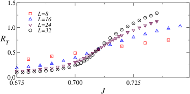
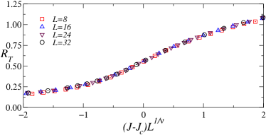
Figure 2: Numerical data for $\gamma=0$ and $w=0.3$. Top: tensor correlation-length ratio $R_{T}$ versus $J$. Bottom: $R_{T}$ versus $(J-J_{c})L^{1/\nu}$, with $J_{c}=0.7097$ and the O(3) critical exponent $\nu\approx 0.7117$.

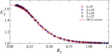
Figure 3: Numerical data for $\gamma=0$ and $w=0.3$. We report $U_{T}$ versus $R_{T}$ and the universal scaling curve $U_{T}(R_{T})$, defined in Eq. (31), for the O(3) vector model (Eq. (46) in the Appendix).

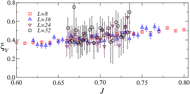
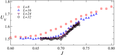
Figure 4: Numerical data for $\gamma=0$ and $w=0.3$. Results for $\xi_{V}$ (top) and $U_{V}$ (bottom) as a function of $J$ across the transition, which show that the vector degrees of freedom are disordered in the whole critical region.

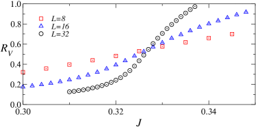
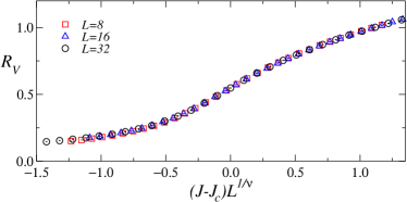
Figure 5: Numerical data for $\gamma=0$ and $w=2.25$. Top: Vector correlation-length ratio $R_{V}$ versus $J$. Bottom: $R_{V}$ versus $(J-J_{c})L^{1/\nu}$, using $J_{c}=0.3270$ and the O(4) critical exponent $\nu=0.750$.

We start the numerical investigation of the phase diagram of the model with Hamiltonian (12), by studying the critical behavior in the small-$w$ region, where we expect transitions to belong to the DT line. Since for $J=\infty$ the tensor-ordered phase corresponds to $w<w_{c}\approx 0.454$, we perform simulations keeping $w=0.3<w_{c}$ fixed and varying $J$. We observe criticality in the tensor channel for $J\approx 0.71$, see the upper panel in Fig. 2. The data for $R_{T}$ are fully consistent with an O(3) critical behavior, as it is evident from the lower panel where we show a scaling plot using the O(3) critical exponent $\nu$ and the estimate $J_{c}=0.7097(1)$ of the critical point. Stronger evidence for O(3) behavior is provided in Fig. 3, where data for $U_{T}$ are reported as a function of $R_{T}$ and compared with the universal curve of the O(3) vector model, obtaining excellent agreement.

Finally, we check that vector degrees of freedom are not critical at the transition: for all the values of $J$ studied, $\xi_{V}$ is very small, see Fig. 4, and the same is true for the susceptibility $\chi_{V}$, which takes the value $\chi_{V}\approx 1.9$ in the transition region (not shown); note that $\chi_{V}=1$ for every $J$ when $w=0$. The vector Binder parameter $U_{V}$ is also reported in Fig. 4. As expected, it is approximately equal to 3/2 in the disordered phase, see Eq. (41), and increases towards to XY value 2 as J increases.

We next investigate the behavior for large $w$ values, where we expect the DV line. Vector and tensor correlations should simultaneously order, displaying O(4) vector critical behavior. Again we perform simulations at fixed $w$, choosing $w=2.25$.

In Fig. 5 we show $R_{V}$ as a function of $J$: a transition is identified for $J=J_{c}=0.3270(1)$. The data show very good scaling when plotted against $(J-J_{c})L^{1/\nu}$, using the O(4) exponent $\nu=0.750$. The O(4) nature of the transition is further confirmed by the plots of $U_{V}$ and $U_{T}$ versus $R_{V}$ and $R_{T}$, respectively, shown in Fig. 6. The numerical data fall on top of the scaling curves $U_{V}(R_{V})$ and $U_{T}(R_{T})$ computed in the O(4) vector model.

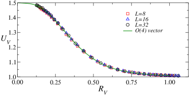
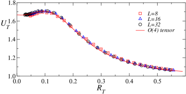
Figure 6: Numerical data for $\gamma=0$ and $w=2.25$. Plots of $U_{V}$ versus $R_{V}$ (top) and of $U_{T}$ versus $R_{T}$ (bottom). The numerical data are compared with the universal scaling curves $U_{V}(R_{V})$ (top) and $U_{T}(R_{T})$ (bottom), defined in Eq. (31), computed in the O(4) vector model (Eqs. (47) and (48) in the Appendix).

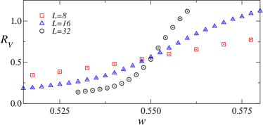
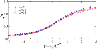
Figure 7: Numerical data for $\gamma=0$ and $J=1$. Top: Vector correlation-length ratio $R_{V}$ versus $w$. Bottom: $R_{V}$ versus $(w-w_{c})L^{1/\nu}$, using the O(2) value $\nu=0.6717$. The critical point is located at $w_{c}=0.5505(3)$.

Finally, we performed a set of simulations, to investigate the nature of the TV line, that separates the two phases in which the tensor degrees of freedom are ordered. As discussed in Sec. IV.5, the TV line can be identified using vector observables that should display O(2) critical behavior. Given that the DT line ends at $J_{c}=0.7102$, $w=0$, we fixed $J=1$ and increased $w$. As evident from Fig. 1, this choice should allow us to observe the TV line.

In Fig. 7, we report $R_{V}$ versus $w$. A crossing point is detected for $w_{c}\approx 0.5505$. Close to it, vector data are fully consistent with an O(2) critical behavior. This is further confirmed by the results reported in Fig. 8. The data of the vector Binder parameter, when plotted versus $R_{V}$, are fully consistent with the corresponding universal curve computed in the vector O(2) model. As a further check that the transition belongs to the TV line, in Fig. 9 we report $U_{T}$ versus $J$: $U_{T}$ converges to 1 by increasing the size of the lattice on both sides of the transition, confirming that tensor modes are fully magnetized.

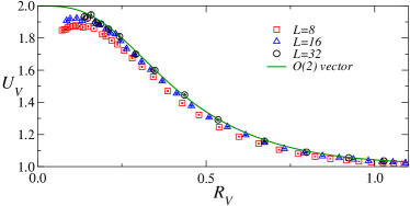
Figure 8: Numerical data for $\gamma=0$ and $J=1$. We report $U_{V}$ versus $R_{V}$ and the universal scaling curve $U_{V}(R_{V})$, defined in Eq. (31), for the O(2) vector model (Eq. (45) in the Appendix).

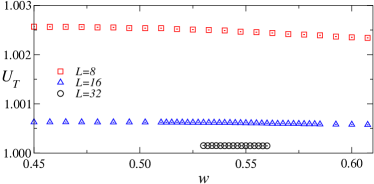
Figure 9: Numerical data for $\gamma=0$ and $J=1$. Estimates of $U_{T}$ versus $w$ across the transition: the tensor degrees of freedom are ordered on both sides of the transition [$w_{c}=0.5505(3)$].

V.2 Simulations in the presence of an axial gauge fixing

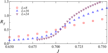
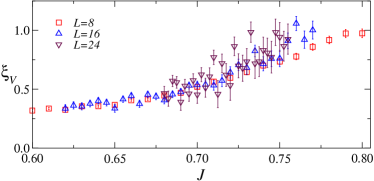
Figure 10: Numerical data for $\gamma=0$ and $w=0.1$, in the axial gauge with $C^{*}$ boundary conditions. Behavior of $R_{T}$ (top) and $\xi_{V}$ (bottom) across the transition [$J_{c}=0.706(1)$]. While a crossing point for $R_{T}$ is clearly seen, vector degrees of freedom are disordered for all values of $J$.

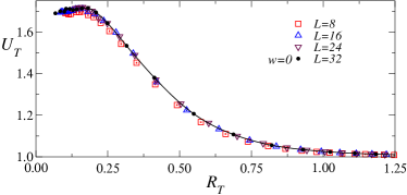
Figure 11: Numerical data for $\gamma=0$ and $w=0.1$, in the axial gauge with $C^{*}$ boundary conditions. The estimates of $U_{T}$ versus $R_{T}$ obtained for $w=0.1$ (results for $L=8,16,24$) are compared with results for the gauge-invariant model with $w=0$ (results for $L=32$). The continuous line is a spline interpolation of the $w=0$ data. The consistency of the data signals that the two transitions belong to the same O(3) universality class.

We now discuss the extended model with Hamiltonian (12) in the presence of the axial gauge fixing. We use C^∗ boundary conditions KW-91 ; LPRT-16 ; BPV-21-gsb , so that we can require $\lambda_{{\bm{x}},3}=1$ on all sites. The purpose of the simulations is that of understanding if a tensor-ordered phase as well as a DT transition line are present, so that gauge invariance is recovered in the critical limit for finite small values of $w$. As we shall see, the answer is positive: the gauge fixing does not change the qualitative shape of the phase diagram.

As we have discussed in Sec. IV.6, even if the qualitative phase diagram is unchanged, the DT phase should shrink and the TV line should get closer to the $w=0$ axis. For this reason, we decided to perform simulations at fixed $w=0.1$. The vector and tensor correlation lengths are reported in Fig. 10 as a function of $J$. The data for $R_{T}$ have a crossing point at $J_{c}=0.706(1)$, which is very close to the critical point for $w=0$, $J_{c}=0.7102(1)$ PV-19-AH3d . The tensor degrees of freedom are critical at the transition. The vector ones are instead disordered and $\xi_{V}$ is of order 1 across the transition. Thus, the data confirm the existence of a DT line also in the presence of the axial gauge fixing. As an additional check, in Fig. 11 we plot $U_{T}$ against $R_{T}$. The data are compared with the results for the gauge-invariant model ($w=0$) with the same C^∗ boundary conditions (we consider results with $L=32$, which should provide a good approximation of the asymptotic curve). The agreement is excellent, confirming that the transition belongs indeed to the DT line, where O(3) behavior is expected. As a side remark, note that the O(3) curves reported in Figs. 11 and 3 are different, since the scaling curve depends on the boundary conditions.

We also performed simulation with $w=0.2$. In this case, we observe two very close transitions, that are naturally identified with transitions on the DT and TV line. They provide an approximate estimate of the multicritical point, $w_{mc}\approx 0.2$, $0.69\lesssim J_{mc}\lesssim 0.70$. Note that the size of the tensor-ordered phase is, not surprisingly, significantly smaller than in the absence of gauge fixing. Indeed, in the latter case $w_{mc}\gtrsim w_{c}(J=1)\approx 0.55$.

V.3 Finite $\gamma$ results for the pure gauge model

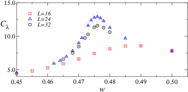
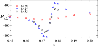
Figure 12: Numerical data for $\gamma=2.5$ and $J=0$ (pure gauge model). Top panel: specific heat $C_{\lambda}$; Bottom panel: third moment $M_{3,\lambda}$.

At $\gamma=\infty$, the phase diagram is characterized by four transition lines, see Sec. IV.3. In addition to the lines reported in Fig. 1, there is a line where $\lambda_{{\bm{x}},\mu}$ is critical and which separates two phases with no tensor or vector order. As we have discussed in Sec. IV.5, such a line is not expected to occur at $\gamma=0$. We wish now to provide evidence that such a line does not exist for any finite $\gamma$. As this line starts on the $J=0$ line, we consider the pure gauge model with Hamiltonian

$$H=H_{\lambda}(\lambda)+H_{b}(\lambda).$$ (43)

For $\gamma=\infty$, there is an XY transition for $w=w_{c,XY}\approx 0.454$. We wish now to verify whether there is a transition for large, but finite values of $\gamma$. If it were present, it would imply the presence of a fourth transition line in the phase diagram. For this purpose, we have studied the model for $\gamma=2.5$. For this value of $\gamma$ the gauge fields are significantly ordered and indeed $\langle\Pi_{{\bm{x}},\mu\nu}\rangle\approx 0.93$ in the relevant region $w\approx w_{c,XY}$. To detect the transition, we have considered cumulants of the energy

$$C_{\lambda} = {1\over Vw^{2}}\langle(H_{b}-\langle H_{b}\rangle)^{2}\rangle,$$

$$M_{3,\lambda} = {1\over Vw^{3}}\langle(H_{b}-\langle H_{b}\rangle)^{3}\rangle.$$ (44)

At an XY transition, the specific heat has a nondiverging maximum while the third cumulant should have a positive and a negative peak SSNHS-03 , both diverging as $L^{3/\nu-3}=L^{(1+\alpha)/\nu}\approx L^{1.47}$. In Fig. 12, we show the two quantities as a function of $w$. The specific heat has a maximum at $w\approx 0.476$, which might in principle signal an XY transition. However, $M_{3,\lambda}$ is not diverging. It increases significantly as $L$ changes from 16 to 24, but its maxima decrease as $L$ varies from 24 to 32. We are evidently observing a crossover behavior, due to the transition present for infinite $\gamma$. Simulations do not provide evidence of finite-$\gamma$ transitions and therefore, of a fourth transition line in the phase diagram.

VI Conclusions

In this work we discuss the role of GSB perturbations in lattice gauge models. In Ref. BPV-21-gsb we studied the AH model with noncompact gauge fields, analyzing the role of GSB perturbations at transitions associated with a charged FP, i.e., where both scalar-matter and gauge correlations are critical. In that case we showed that there is an extreme sensitivity of the system to GSB perturbations, such as the photon mass in the AH field theory. In this work, instead, we discuss the behavior at transitions where gauge correlations are not critical and the gauge symmetry has only the role of reducing the scalar degrees of freedom that display critical behavior. A paradigmatic model in which this type of behavior is observed is the 3D lattice CP¹ model or, more generally, the lattice AH model with two-component complex scalar matter and U(1) compact gauge fields. We find that in this case, the critical gauge-invariant modes are robust against GSB perturbations: for small values of the GSB coupling, the critical behavior (continuum limit) is the same as in the gauge-invariant model.

Note that, even when gauge symmetry is explicitly broken, the existence of a gauge-symmetric limit is very useful to understand the physics of the model. If indeed one directly studies the gauge-broken model, a detailed analysis of the nonperturbative dynamics of the model would be required to identify the nature of the critical degrees of freedom, which instead emerges naturally in the gauge-invariant limit. Looking for gauge-invariant limits or deformations might thus be a useful general strategy to pursue in order to understand the origin of “unusual” orderings and transitions (the DT and the TV lines in the present model or in the models with Hamiltonians (18) and (23)).

In our study we consider the $N=2$ lattice AH model with Hamiltonian (2). The model has two phases PV-19-AH3d separated by a continuous transition line driven by the condensation of the gauge-invariant operator $Q$ defined in Eq. (11). The nature of the transition is independent of the gauge coupling and the is same as that in the CP¹ model, which, in turn, is the same as that in the O(3) vector model.

We add to the Hamiltonian (2) the GSB term $H_{b}=-w\sum_{{\bm{x}},\mu}{\rm Re}\,\lambda_{{\bm{x}},\mu}$, where the parameter $w$ quantifies the strength of the perturbation. A detailed numerical MC study, supported by the analysis of some limiting cases, allows us to determine the phase diagram of the model, see Fig. 1. Its main features are summarized as follows.

• The parameter $w$ is an irrelevant RG perturbation of the gauge-invariant critical behavior (continuum limit). Therefore, even in the presence of a finite small GSB perturbation, the critical behavior is the same as that of the gauge-invariant CP¹ universality class. The gauge-breaking effects of the linear perturbation disappear in the large-distance behavior.

• As sketched in Fig. 1, the phase diagram of the model with Hamiltonian Eq. (12) presents three phases for $\gamma=0$: a disordered phase for small $J$ and two ordered phases for large $J$. There is a tensor-ordered phase for small values of $w$, in which the operator $Q$ defined in Eq. (11) condenses, while the vector correlation $G_{V}$ defined in Eq. (24) is short ranged. For sufficiently large values of $w$, the ordered phase is characterized by the condensation of the vector matter field.

  The three phases are separated by three different transition lines that presumably meet at a multicritical point. It would be interesting to understand its nature, but we have not pursued this point further.

  Most of our results are obtained for the case $\gamma=0$, i.e., for the CP¹ model, but we expect the same phase diagram also for any finite $\gamma$, with strong crossover effects for large values of $\gamma$.

• Transitions along the DT line, that separates the disordered phase from the tensor-ordered phase, belong to the O(3) vector universality class, as the transition for $w=0$.

• Transitions along the DV line, that separates the disordered phase from the vector-ordered phase, belong to the O(4) vector universality class BPV-21-gsb . Note the effective symmetry enlargement at the transition—from U(2) to O(4)—that was predicted using RG arguments based on the correspoding LGW theory BPV-21-gsb . Of course, the symmetry enlargement is limited to the critical regime. Outside the critical region, one can only observe the global U(2) symmetry of the model.

• Transitions along the TV line, that separates the tensor and the vector ordered phases, are associated with the condensation of the global phase of the scalar field, which is disordered in the tensor-ordered phase and ordered in the vector-ordered phase. Continuous transitions along the TV line belong to the O(2) or XY universality class. Note that this mechanism realizes an unusual phenomenon: two ordered phases are separated by a continuous transition line.

• We have also studied the model in the presence of a gauge fixing. We considered the axial gauge fixing defined in Eq. (22). We find the phase diagram to be qualitatively similar to that found in the absence of a gauge fixing, see Fig. 1. In particular, for sufficiently small $w$, the critical behavior is the same as in the gauge-invariant theory.

We have not analyzed the behavior for $N>2$. Also in this case, we expect a phase diagram with three different phases, as for $N=2$. However, the nature of the transition lines might be different. Since the transitions in the gauge-invariant lattice CP^N-1 models are of first-order for any $N>2$, the transitions along the DT line should be of first order. Transitions along the TV line should still belong to the XY universality class, if they are continuous, while transitions along the DV line are expected to belong to the O($2N$) vector universality class with the effective enlargement of the symmetry of the critical modes from U($N$) to O($2N$).

There are several interesting extension of our work. One might consider GSB terms involving higher powers of the link variables, for instance $H_{b,q}=-w\sum_{{\bm{x}},\mu}{\rm Re}\,\lambda_{{\bm{x}},\mu}^{q}$, which leave a residual discrete ${\mathbb{Z}}_{q}$ gauge symmetry. In this case we may have a more complex phase diagram where the residual gauge symmetry may play a role. One may also consider the same linear perturbation in the AH model with higher-charge compact matter fields BPV-20-q2 , which has a more complex phase diagram than the AH lattice model we consider here.

Finally, we mention that several nonabelian gauge models with multiflavor scalar matter BPV-19-sqcd ; BPV-20-son ; BFPV-21-adj have transitions where gauge correlations do not become critical. Gauge symmetry is only relevant for defining the critical modes and therefore the symmetry-breaking pattern associated with the transition, as in the lattice AH model we have considered here. For this class of nonabelian models, one might investigate the role of similar GSB terms, for instance of a perturbation $H_{b}=-w\sum_{{\bm{x}},\mu}\hbox{Re Tr}\,U_{{\bm{x}},\mu}$ where $U_{{\bm{x}},\mu}$ are the gauge variables associated with the lattice links Wilson-74 , to understand whether a gauge-invariant continuum limit is still obtained for small values of $w$.

Appendix A Universal scaling curve in O($N$) vector models

In this Appendix we collect the expressions of the scaling curves $F_{U}(R)$, defined in Eq. (31), for periodic boundary conditions and cubic lattices $L^{3}$, computed in the O(2), O(3), and O(4) vector models. We report here some simple parametrizations. The error on these expressions should be less than 0.5%.

On the TV line, the vector data have been compared with analogous vector data computed in the XY model. The XY curve $U_{V}=F_{U}(R_{V})$ is given by

$$F_{U}(x)=2$$

$$\qquad+27.508562x^{2}-216.397337x^{3}+360.327374x^{4}$$

$$\qquad-307.205086x^{5}+133.83076x^{6}-23.718357x^{7}$$

$$\qquad-(1-e^{-7x^{2}})(4.038703-5.785571x)$$

$$\qquad+22.958929x^{2}(1-e^{-8x}),$$ (45)

valid for $x<1.1$.

Along the DT line, the scaling curve $U_{T}=F_{U}(R_{T})$ in the tensor sector is the same as the scaling curve in the O(3) model for vector quantities (i.e., computed using correlations of $m^{a}=\sum_{x}s^{a}_{\bm{x}}$, where $s^{a}_{\bm{x}}$ is a three-dimensional unit spin):

$$F_{U}(x)={5\over 3}-47.83889x^{2}+58.48967x^{3}-67.02068x^{4}$$

$$\qquad+38.408855x^{5}-8.8557348x^{6}$$

$$\qquad+x(3.0263535+23.139470x)(1-e^{-15x}),$$ (46)

valid for $x<1.0$.

Finally, the scaling curves $U_{V}=F_{U}(R_{V})$ and $U_{T}=F_{U}(R_{T})$ along the DV line can be computed in the O(4) model. The vector curve $U_{V}=F_{U}(R_{V})$ corresponds to the vector curve in the O(4) model, which can be parametrized as

$$F_{U}(x)={3\over 2}-48.804243x^{2}+64.371024x^{3}$$

$$\qquad-85.177814x^{4}+62.735307x^{5}$$

$$\qquad-24.558342x^{6}+3.998991x^{7}$$

$$\quad+x(3.039763+23.904433x)(1-e^{-15x}),$$ (47)

valid for $x<1.0$. The tensor curve $U_{T}=F_{U}(R_{T})$ for the tensor operator $Q$ can also be related to an O(4) scaling curve. The relation is discussed in App. B of Ref. PV-19-AH3d . We parametrize the O(4) results as

$$F_{U}(x)={5\over 3}-2077.568536x^{2}+6198.556568x^{3}$$

$$\quad-15494.694968x^{4}+22321.613611x^{5}$$

$$\quad-17453.201432x^{6}+5754.439605x^{7}$$

$$+x(128.626365+713.495184x)(1-e^{-16x}),$$ (48)

valid for $x<0.6$.

References

- (1) K. G. Wilson, Confinement of quarks, Phys. Rev. D 10, 2445 (1974).
- (2) S. Weinberg, The Quantum Theory of Fields, (Cambridge University Press, 2005).
- (3) J. Zinn-Justin, Quantum Field Theory and Critical Phenomena, fourth edition (Clarendon Press, Oxford, 2002).
- (4) X.-G. Wen, Quantum field theory of many-body systems: from the origin of sound to an origin of light and electrons, (Oxford University Press, 2004)
- (5) P. W. Anderson, Superconductivity: Higgs, Anderson and all that, Nat. Phys. 11, 93 (2015).
- (6) S. Gazit, F. F. Assaad, S. Sachdev, A. Vishwanath, and C. Wang, Confinement transition of gauge theories coupled to massless fermions: emergent QCD3 and SO(5) symmetry, Proceedings of the National Academy of Sciences 115, E6987 (2018).
- (7) S. Sachdev, Topological order, emergent gauge fields, and Fermi surface reconstruction, Rep. Prog. Phys. 82, 014001 (2019).
- (8) S. Sachdev, H. D. Scammell, M. S. Scheurer, and G. Tarnopolsky, Gauge theory for the cuprates near optimal doping, Phys. Rev. B 99, 165126 (2019).
- (9) H. Goldman, R. Sohal, and E. Fradkin, Landau-Ginzburg Theories of Non-Abelian Quantum Hall States from Non-Abelian Bosonization, Phys. Rev. B 100, 115111 (2019).
- (10) C. Wetterich, Gauge symmetry from decoupling, Nucl. Phys. B 915, 135 (2017).
- (11) D. Foerster, H. B. Nielsen, and N. Ninomiya, Dynamical stability of local gauge symmetry, Phys. Lett. B 94, 135 (1980).
- (12) J. Iliopoulos, D. V. Nanopoulos, and T. N. Tomaras, Infrared stability of anti-grandunification, Phys. Lett. B 94, 141 (1980).
- (13) E. Zohar, J. I. Cirac, and B. Reznik, Quantum simulations of lattice gauge theories using ultracold atoms in optical lattices, Rep. Prog. Phys. 79, 014401 (2015).
- (14) M. C. Bañuls, et al, Simulating lattice gauge theories with quantum technologies, Eur. Phys. J. D. 74, 165 (2020).
- (15) M. C. Bañuls and K. Cichy, Review on novel methods for lattice gauge theories, Rep. Prog. Phys. 83, 024401 (2020).
- (16) C. Bonati, A. Pelissetto, and E. Vicari, Lattice Abelian-Higgs model with noncompact gauge fields, Phys. Rev. B 103, 085104 (2021).
- (17) C. Bonati, A. Pelissetto, and E. Vicari, Breaking of the gauge symmetry in lattice gauge theories, arXiv:2104.09892.
- (18) B. I. Halperin, T. C. Lubensky, and S. K. Ma, First-Order Phase Transitions in Superconductors and Smectic-A Liquid Crystals, Phys. Rev. Lett. 32, 292 (1974).
- (19) R. Folk and Y. Holovatch, On the critical fluctuations in superconductors, J. Phys. A 29, 3409 (1996).
- (20) B. Ihrig, N. Zerf, P. Marquard, I. F. Herbut, and M. M. Scherer, Abelian Higgs model at four loops, fixed-point collision and deconfined criticality, Phys. Rev. B 100, 134507 (2019).
- (21) M. Moshe and J. Zinn-Justin, Quantum field theory in the large limit: A review, Phys. Rep. 385, 69 (2003).
- (22) A. Pelissetto and E. Vicari, Three-dimensional ferromagnetic CPN-1 models, Phys. Rev. E 100, 022122 (2019).
- (23) S. Takashima, I. Ichinose, and T. Matsui, CP1+U(1) lattice gauge theory in three dimensions: Phase structure, spins, gauge bosons, and instantons, Phys. Rev. B 72, 075112 (2005).
- (24) S. Takashima, I. Ichinose, and T. Matsui, Deconfinement of spinons on critical points: Multiflavor CP1+U(1) lattice gauge theory in three dimension, Phys. Rev. B 73, 075119 (2006).
- (25) A. Pelissetto and E. Vicari, Multicomponent compact Abelian-Higgs lattice models, Phys. Rev. E 100, 042134 (2019).
- (26) M. Creutz, Quarks, Gluons and Lattices (Cambridge, Cambridge University press, 1985).
- (27) C. Itzykson and J. Drouffe, Statistical field theory (Cambridge, Cambridge University Press, 1989).
- (28) A. S. Kronfeld and U. J. Wiese, SU(N) gauge theories with C periodic boundary conditions. 1. Topological structure, Nucl. Phys. B 357, 521 (1991).
- (29) B. Lucini, A. Patella, A. Ramos and N. Tantalo, Charged hadrons in local finite-volume QED+QCD with C∗ boundary conditions, JHEP 02, 076 (2016).
- (30) A. Pelissetto and E. Vicari, Critical Phenomena and Renormalization Group Theory, Phys. Rep. 368, 549 (2002).
- (31) M. Hasenbusch, Monte Carlo study of a generalized icosahedral model on the simple cubic lattice, Phys. Rev. B 102, 024406 (2020).
- (32) S. M. Chester, W. Landry, J. Liu, D. Poland, D. Simmons-Duffin, N. Su, and A. Vichi, Bootstrapping Heisenberg magnets and their cubic instability, arXiv:2011.14647.
- (33) M. V. Kompaniets and E. Panzer, Minimally subtracted six-loop renormalization of -symmetric theory and critical exponents, Phys. Rev. D 96, 036016 (2017).
- (34) M. Hasenbusch and E. Vicari, Anisotropic perturbations in 3D O(N) vector models, Phys. Rev. B 84, 125136 (2011).
- (35) M. Campostrini, M. Hasenbusch, A. Pelissetto, P. Rossi, and E. Vicari, Critical exponents and equation of state of the three-dimensional Heisenberg universality class, Phys. Rev. B 65, 144520 (2002).
- (36) R. Guida and J. Zinn-Justin, Critical exponents of the -vector model, J. Phys. A 31, 8103 (1998).
- (37) A. Pelissetto, E. Vicari, Large- behavior of three-dimensional lattice CPN-1 models, J. Stat. Mech. (2020) 033209.
- (38) H. G. Ballesteros, L. A. Fernandez, V. Martín-Mayor, A. Muñoz Sudupe, Finite size effects on measures of critical exponents in O() models, Phys. Lett. B 387, 125 (1996).
- (39) M. Campostrini, A. Pelissetto, P. Rossi, E. Vicari, Four-point renormalized coupling in O() models, Nucl. Phys. B 459, 207 (1996).
- (40) P. Butera and M. Comi, -vector spin models on the sc and the bcc lattices: a study of the critical behavior of the susceptibility and of the correlation length by high temperature series extended to order , Phys. Rev. B 56, 8212 (1997).
- (41) M. Hasenbusch, O() and RPN-1 models in two dimensions, Phys. Rev. D 53, 3445 (1996).
- (42) M. Campostrini, M. Hasenbusch, A. Pelissetto, and E. Vicari, Theoretical estimates of the critical exponents of the superfluid transition in 4He by lattice methods, Phys. Rev. B 74, 144506 (2006).
- (43) Y. Deng, H. W. J. Blöte, and M, Nightingale, Surface and bulk transitions in three-dimensional models, Phys. Rev. E 72, 016128 (2005).
- (44) M. Hasenbusch, Monte Carlo study of an improved clock model in three dimensions, Phys. Rev. B 100, 224517 (2019).
- (45) S. M. Chester, W. Landry, J. Liu, D. Poland, D. Simmons-Duffin, N. Su, and A. Vichi, Carving out OPE space and precise O(2) model critical exponents, J. High Energy Phys. 06, 142 (2020).
- (46) J. Smiseth, E. Smørgrav, F. S. Nogueira, J. Hove, and A. Sudbø, Phase Structure of Compact Lattice Gauge Theories and the Transition from Mott Insulator to Fractionalized Insulator, Phys. Rev. B 67, 205104 (2003).
- (47) C. Bonati, A. Pelissetto, E. Vicari Higher-charge three-dimensional compact lattice Abelian-Higgs models Phys. Rev. E 102, 062151 (2020).
- (48) C. Bonati, A. Pelissetto, and E. Vicari, Phase Diagram, Symmetry Breaking, and Critical Behavior of Three-Dimensional Lattice Multiflavor Scalar Chromodynamics, Phys. Rev. Lett. 123, 232002 (2019); Three-dimensional lattice multiflavor scalar chromodynamics: Interplay between global and gauge symmetries, Phys. Rev. D 101. 034505 (2020).
- (49) C. Bonati, A. Pelissetto, and E. Vicari, Three-dimensional phase transitions in multiflavor scalar SO() gauge theories, Phys. Rev. E 101, 062105 (2020).
- (50) C. Bonati, A. Franchi, A. Pelissetto, and E. Vicari, Three-dimensional lattice SU() gauge theories with multiflavor scalar matter in the adjoint representation, in preparation.