A topological characterisation of the Kashiwara–Vergne groups

Abstract.

In [BND17] Bar-Natan and the first author show that solutions to the Kashiwara–Vergne equations are in bijection with certain knot invariants: homomorphic expansions of welded foams. Welded foams are a class of knotted tubes in $\mathbb{R}^{4}$, which can be finitely presented algebraically as a circuit algebra, or equivalently, a wheeled prop. In this paper we describe the Kashiwara-Vergne groups $\mathsf{KV}$ and $\mathsf{KRV}$ – the symmetry groups of Kashiwara-Vergne solutions – as automorphisms of the completed circuit algebras of welded foams, and their associated graded circuit algebras of arrow diagrams, respectively. Finally, we provide a description of the graded Grothendieck-Teichmüller group $\mathsf{GRT}_{1}$ as automorphisms of arrow diagrams.

1. Introduction

Universal finite type invariants, or homomorphic expansions, are powerful tools in the study of knots and three-manifolds. Given a class of knotted objects $\mathcal{K}$, an expansion $Z:\mathcal{K}\rightarrow\mathsf{A}$ takes values in the associated graded space of $\mathcal{K}$ with respect to a Vassiliev filtration, and satisfies the universality property that the associated graded map of $Z$ is the identity map of $\mathsf{A}$. An expansion is homomorphic if it respects any operations defined on $\mathcal{K}$, such as braid or tangle composition, knot connected sum or cabling. The space $\mathsf{A}$ is usually combinatorially described as Jacobi or Feynman diagrams. The most famous class of examples is the Kontsevich integral of knots [Kon93], and its many variants [BN13], [BN95], [LM96], [LMO98].

In practice, producing homomorphic expansions is often difficult, and in many cases (e.g. for tangles) they don’t exist. When $\mathcal{K}$ can be finitely presented as an algebraic structure (e.g. parenthesised braids viewed as a category), the Vassiliev filtration coincides with the $I$-adic filtration by powers of the augmentation ideal, and finding a homomorphic expansion is equivalent to solving a set of equations in the associated graded space $\mathsf{A}$. In this vein, Bar-Natan [BN98] showed that there is a bijection between homomorphic expansions for parenthesised braids and Drinfeld associators: objects in quantum algebra defined as the set of solutions to the pentagon and hexagon equations. The existence of homomorphic expansions for parenthesised braids can thus be inferred from the existence of Drinfeld associators.

In [Dri90], Drinfeld introduced two groups, the Grothendieck–Teichmüller group $\mathsf{GT}$ and its graded version $\mathsf{GRT}_{1}$, which act freely and transitively on the set of associators. Bar-Natan’s homomorphic expansions induce isomorphisms between the prounipotent completion of parenthesised braids, $\widehat{\mathsf{PaB}}$, and their associated graded parenthesised chord diagrams, $\mathsf{PaCD}$. As such, Bar-Natan [BN98] showed that it is natural to identify these symmetry groups with automorphisms of the source and target so that

$$\mathsf{GT}\cong\operatorname{Aut}(\widehat{\mathsf{PaB}})\quad\text{and}\quad\mathsf{GRT}_{1}\cong\operatorname{Aut}(\mathsf{PaCD}),$$

which act freely and transitively on homomorphic expansions by pre- and post-composition respectively. Later, several authors noticed that the collections of parenthesised braids and parenthesised chord diagrams could be concisely described as operads, and that homomorphic expansions, and therefore Drinfeld associators, can be identified with the set of operad isomorphisms $Z:\widehat{\mathsf{PaB}}\rightarrow\mathsf{PaCD}$ ([Tam98], [Fre17a]).

A higher-dimensional version of Bar-Natan’s story arises in the Lie theoretic context of the Kashiwara–Vergne problem. Informally, the Kashiwara–Vergne conjecture asks when, in the non-commutative setting, one can simplify the exponentiation rule

$$e^{x}e^{y}=e^{\mathfrak{bch}(x,y)}.$$

Here, we write

$$\mathfrak{bch}(x,y)=x+y+\frac{1}{2}[x,y]+\frac{1}{12}[x,[x,y]]+\dots$$

for the Baker–Campbell–Hausdorff series. While the Baker–Campbell–Hausdorff series provides a formula for $e^{x}e^{y}$ as an infinite Lie series, this is not always useful in applications. The original form of the Kashiwara–Vergne (KV) conjecture [KV78] asks if the Baker-Campbell-Hausdorff series can be expressed in terms of a convergent power series and adjoint endomorphisms. A solution to the KV conjecture can be formulated as an automorphism $F$ of the (degree completed) free Lie algebra $\widehat{\mathfrak{lie}}_{2}$ with generators $x$ and $y$, such that $F$ satisfies the first KV equation

$$F(e^{x}e^{y})=e^{x+y},$$

as well as several other properties which we omit here (complete details in Section 5).

The existence of general solutions to the KV conjecture was shown in 2006 [AM06] and a deep relationship between the KV conjecture and Drinfeld associators was established in [AT12, AET10]. As in the case of Drinfeld associators, there exist symmetry groups, called the Kashiwara–Vergne groups and denoted $\mathsf{KV}$ and $\mathsf{KRV}$, which act freely and transitively on the set of solutions to the KV equations.

As with Drinfeld associators, the set of KV solutions has a topological description. Welded foams, heretofore called $w$-foams, are a class of knotted surfaces in $\mathbb{R}^{4}$ [Sat00]. They have much in common with parenthesised braids, but live in a higher dimension. In a series of papers [BND16, BND17], Bar-Natan and the first author show that homomorphic expansions of $w$-foams are in bijection with the solutions to the KV conjecture [BND17, Theorem 4.9]. The existence of a homomorphic expansion for $w$-foams can therefore be deduced from the existence of solutions to the KV conjecture. In this paper, we build on this topological interpretation of the KV conjecture to give a simultaneously topological and “operadic” interpretation of the Kashiwara–Vergne groups.

A key feature of $w$-foams is that they are finitely presented as a circuit algebra with additional cabling-type operations called unzips. Circuit algebras, reviewed in Section 2.1, are a generalisation of Jones’s planar algebras [Jon99], in which one drops the planarity condition on “connection diagrams”. We describe circuit algebras as algebras over the coloured operad of wiring diagrams in Definition 2.3. Alternatively, in [DHR21, Theorem 5.5] we showed that circuit algebras are equivalent to a type of tensor category called a wheeled prop. The preliminary sections of this paper describe the circuit algebra of $w$-foams, denoted $\mathsf{wF}$, as well as its associated graded circuit algebra $\mathsf{A}$, where homomorphic expansions take values. $\mathsf{A}$ admits a combinatorial description in terms of arrow diagrams (Definition 3.3): an oriented version of the better known space of chord diagrams. The first main theorem of this paper is the following (Theorem 5.12):

Theorem.

There is an isomorphism of groups $\operatorname{Aut}_{v}(\mathsf{A})\cong\mathsf{KRV}$.

In order to develop the corresponding theorem for the group $\mathsf{KV}$, we construct a prounipotent completion of the circuit algebra of $w$-foams. We show explicitly that completion intertwines with the circuit algebra operations, as well as unzips and the further auxiliary operations. In this way, we avoid a full development of the rational homotopy theory of circuit algebras which arises in the operadic approach to the Grothendieck-Teichmüller group (e.g. Fresse [Fre17b]). The decision to avoid rational homotopy theory for circuit algebras is due to the fact that $w$-foams have a richer structure than that of just a circuit algebra: the most notable additional structure is embodied by the unzip operations. Full details are in Sections 2.2 and 2.3.

After taking the prounipotent completion of $w$-foams, we show that homomorphic expansions correspond to isomorphisms of circuit algebras (Theorem 4.9).

Theorem.

For any homomorphic expansion $Z:\mathsf{wF}\xrightarrow{}\mathsf{A}$, the induced map $\widehat{Z}:\widehat{\mathsf{wF}}\to\mathsf{A}$ is an isomorphism of filtered, complete circuit algebras.

This is a new contribution to the literature on homomorphic expansions of $w$-foams, where completions so far have not been discussed. Current work-in-progress by Bar-Natan [Bar15] further explores the interactions between prounipotent completion and homomorphic expansions for groups. A direct consequence of this result is that we can identify KV solutions with isomorphisms of circuit algebras. Another consequence of Theorem 4.9 is that we can describe the symmetry group $\mathsf{KV}$ as automorphisms of (completed) $w$-foams by combining a (non-canonical) isomorphism $\widehat{Z}$ and the isomorphism $\operatorname{Aut}_{v}(\mathsf{A})\cong\mathsf{KRV}$ in Theorem 5.16:

Theorem.

There is an isomorphism of groups $\operatorname{Aut}_{v}(\widehat{\mathsf{wF}})\cong\mathsf{KV}$.

These results complete the $4$-dimensional topological interpretation of the Kashiwara–Vergne conjecture initiated by Bar-Natan and the first author. At the same time, combining these results with the wheeled prop description of circuit algebras [DHR21], we have given an “operadic” interpretation of the Kashiwara-Vergne groups. Namely, solutions of the Kashiwara–Vergne conjecture give rise to isomorphisms of completed wheeled props, and the symmetry groups $\mathsf{KV}$ an $\mathsf{KRV}$ are identified with automorphism groups of completed wheeled props.

The parallels between Drinfeld associators and Kashiwara–Vergne solutions are more than a coincidence. In a series of breakthrough articles Alekseev, Enriquez and Torossian [AT12, AET10] show that each Drinfeld associator $\Phi$ ([Dri90, Dri89]) gives rise to a KV solution $F_{\Phi}$. Conversely, a KV solution $F$ gives rise to a “KV associator” $\Phi_{F}$. The main distinction is that KV associators live in a different space than Drinfeld associators: KV associators are automorphisms of free Lie algebras and Drinfeld associators are automorphisms of Lie algebras of infinitesimal braids.

This close relationship extends to a relationship between the graded Grothendieck–Teichmüller group $\mathsf{GRT}_{1}$ and the graded Kashiwara–Vergne group $\mathsf{KRV}$. Alekseev and Torossian construct a group homomorphism $\varrho:\mathsf{GRT}_{1}\rightarrow\mathsf{KRV}$ and conjecture that $\mathsf{KRV}\cong\mathsf{GRT}_{1}\times\mathbb{Q}$ [AT12, Remark 9.14]. It is natural to wish to interpret this relationship in the topological and operadic context. In Section 6, we describe the relationship between the operad of parenthesised chord diagrams $\mathsf{PaCD}$ and the circuit algebra of arrow diagrams $\mathsf{A}$. Because the algebraic structures are different– $\mathsf{PaCD}$ is an operad and $\mathsf{A}$ a circuit algebra– the relationship is subtle. Nonetheless, we construct an image of $\mathsf{PaCD}$ in $\mathsf{A}$, and exhibit $\mathsf{GRT}_{1}$ as automorphisms of arrow diagrams in Theorem 6.10.

Remark 1.1.

The topological interpretation of the analogous map $\varrho:\mathsf{GT}_{1}\rightarrow\mathsf{KV}$ which maps the prounipotent radical of the Grothendieck–Teichmüller group into the Kashiwara–Vergne group $\mathsf{KV}$ ([AET10]) is not included in this paper, but is the topic of separate, future work.

Acknowledgements

The authors would like to thank Dror Bar-Natan, who has been generous with his insights throughout the writing of this paper, and contributed important ideas to several proofs. We also thank Anton Alekseev, Tamara Hogan, Arun Ram, and Chris Rogers for their interest, suggestions and helpful mathematical discussions. The first and third author would like to thank the Mathematical Sciences Research Institute (MSRI) for their support via the 2020 program "Higher Categories and Categorification" and the Sydney Mathematical Research Institute (SMRI) for providing visitor funding to the third author, and a constructive working environment where much of this paper was written.

2. Preliminaries

2.1. Circuit algebras

A circuit algebra is an algebraic structure analogous to Jones’s planar algebras  [Jon99] used to describe virtual and welded tangles in low-dimensional topology. Informally, an oriented circuit algebra is a bi-graded sequence of sets or vector spaces, together with a family of operations parametrised by wiring diagrams $\mathfrak{D}$. More formally, the collection of all wiring diagrams forms a coloured operad and circuit algebras are algebras over this operad. Here we present the basic details needed in this paper, and refer the reader to [DHR21] for a complete introduction and an alternate, equivalent, description of circuit algebras as wheeled props.

Throughout this section, let $\mathcal{I}$ denote a countable alphabet, the set of labels.

Definition 2.1.

An oriented wiring diagram is a triple $\mathfrak{D}=(\mathcal{L},M,f)$ consisting of:

1. A set of sets of labels

   $$\mathcal{L}=\{L_{0}^{-},L_{0}^{+};L_{1}^{-},L_{1}^{+},\ldots,L_{r}^{-},L_{r}^{+}\}\subseteq\mathcal{I}.$$

   The elements of the set $L^{-}_{i}$ are referred to as the $i$th set of outgoing labels and the elements of $L^{+}_{i}$ are the $i$th set of incoming labels. The sets $L_{0}^{-}$ and $L_{0}^{+}$ play a distinguished role: their elements are called the output labels of the diagram $\mathfrak{D}$, while $L_{i}^{+}$ and $L_{i}^{-}$ for $i>0$ are called input labels. We write $L_{i}^{\pm}$ to mean “$L_{i}^{-}$ and $L_{i}^{+}$, respectively” and we may refer to the set $L_{i}^{\pm}$ as the $i$th label set of $\mathfrak{D}$.

2. An abstract, oriented, compact $1$-manifold $M$ with boundary, $\partial M$, regarded up to orientation-preserving homeomorphism. We write $\partial M^{-}$ for the set of beginning boundary points of $M$, and $\partial M^{+}$ for the set of ending boundary points, so $\partial M=\partial M^{-}\sqcup\partial M^{+}$.

3. Set bijections

   $$\partial M^{-}\xrightarrow{f}\cup^{r}_{i=0}{L^{-}_{i}}\quad\textrm{and}\quad\partial M^{+}\xrightarrow{f}\cup^{r}_{i=0}{L^{+}_{i}}.$$

Wiring diagrams have a convenient pictorial representation as tangle diagrams, as in Figure 1. In this representation, we arrange the elements of $\mathcal{L}$ on the boundary of a disc with $r$ disjoint holes

$$D_{0}\setminus(\mathring{D}_{1}\sqcup\mathring{D}_{2}\sqcup\ldots\sqcup\mathring{D}_{r}).$$

The set $L_{0}^{\pm}$ gives a set of distinguished points on the boundary of the big disc $D_{0}$ and each $L_{i}^{\pm}$ represents a set of distinguished points on the boundary of the $i$th interior disc. The abstract $1$-manifold $M$ is pictured as an immersed $1$-manifold, pairing up the input and output labels from $\mathcal{L}$. While this pictorial representation is convenient, and we will use it throughout the paper, we emphasise that wiring diagrams are combinatorial, not topological objects. In particular, the chosen immersion of the $1$-manifold $M$ depicted in Figure 1 is not part of the wiring diagram data. See [DHR21, Proposition 2.3] for more details.

Figure 1. An example of an oriented wiring diagram. The labels sets are $L_{0}^{-}=\{l_{1},l_{2},l_{4}\}$, $L_{0}^{+}=\{l_{3},l_{5}\}$, $L_{1}^{-}=\{a_{2},a_{3}\}$, $L_{1}^{+}=\{a_{1},a_{4}\}$, $L_{2}^{-}=\{b_{1},b_{2},b_{5}\}$, $L_{2}^{+}=\{b_{3},b_{4}\}$. The manifold, drawn in red lines, is a disjoint union of seven oriented intervals and one oriented circle. We don’t draw arrows on circles, since they are abstract, not embedded: there is only one homeomorphism type of an oriented circle.

Wiring diagrams assemble into a coloured operad. We briefly recall that for a fixed set of colours, $\mathfrak{C}$, a $\mathfrak{C}$-coloured operad $\mathsf{P}=\{\mathsf{P}(c_{0};c_{1},\ldots,c_{r})\}$ consists of a collection of sets $\mathsf{P}(c_{0};c_{1},\ldots,c_{r})$: one for each sequence $c_{0};c_{1},\ldots,c_{r}$ of colours in $\mathfrak{C}$. This is equipped with an $\mathcal{S}_{r}$–action permuting $c_{1},\ldots,c_{r}$, together with an equivariant, associative and unital family of partial compositions

$$\leavevmode\hbox to307.05pt{\vbox to17.42pt{\text{[drawing]}}}, {\circ_{i}:\mathsf{P}(c_{0};c_{1},\ldots,c_{r})\times\mathsf{P}(d_{0};d_{1},\ldots,d_{s})} {\mathsf{P}(c_{0};c_{1},\ldots,c_{i-1},d_{1},\ldots,d_{s},c_{i+1},\ldots,c_{r})} {\circ_{i}:\mathsf{P}(c_{0};c_{1},\ldots,c_{r})\times\mathsf{P}(d_{0};d_{1},\ldots,d_{s})} {\mathsf{P}(c_{0};c_{1},\ldots,c_{i-1},d_{1},\ldots,d_{s},c_{i+1},\ldots,c_{r})}$$

whenever $d_{0}=c_{i}$. For full details see [BM07, Definition 1.1].

We denote the set of all wiring diagrams of type $(L^{\pm}_{0};L^{\pm}_{1},\ldots,L^{\pm}_{r})$ by $\mathsf{WD}(L^{\pm}_{0};L^{\pm}_{1},\ldots,L^{\pm}_{r})$. The set $\mathsf{WD}(L^{\pm}_{0};L^{\pm}_{1},\ldots,L^{\pm}_{r})$ has a natural action by $\mathcal{S}_{r}$ permuting the input label sets, so that for any $\sigma\in\mathcal{S}_{r}$

Definition 2.2.

The collection $\mathsf{WD}=\{\mathsf{WD}(L^{\pm}_{0};L^{\pm}_{1},\ldots,L^{\pm}_{r})\}$ forms a discrete coloured operad called the operad of oriented wiring diagrams with partial compositions as follows. For $\mathfrak{D}=(\mathcal{L},M,f)$ and $\mathfrak{D}^{\prime}=(\mathcal{L}^{\prime},N,g)$, if $L_{i}^{-}=L_{0}^{\prime+}$ and $L_{i}^{+}=L_{0}^{\prime-}$ then $\mathfrak{D}\circ_{i}\mathfrak{D}^{\prime}$ is defined by the label set $\{L_{1}^{\pm},...,L_{i-1}^{\pm},L_{1}^{\prime\pm},...,L_{s}^{\prime\pm},L_{i+1}^{\pm}...L_{r}^{\pm}\}$, the manifold $M\sqcup N/\sim$ obtained from $M$ and $N$ by gluing along the boundary identification $L_{i}^{-}=L_{0}^{\prime+}$ and $L_{i}^{+}=L_{0}^{\prime-}$, and the set bijection $f\sqcup g/\sim$ induced by $f$ and $f^{\prime}$ in the natural way.

Pictorially, wiring diagram composition shrinks the wiring diagram $\mathfrak{D}^{\prime}$ and glues it into the $i$th input circle of $\mathfrak{D}$ in such a way that the labels match and the boundary points of the $1$-manifolds are identified: see Figure 2. Composition in the operad $\mathsf{WD}$ is similar to the operad of planar tangles in [Jon99] and [HPT, Definition 2.1].

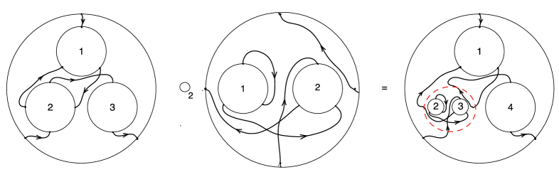
Figure 2. An example of the partial composition of oriented wiring diagrams.

An oriented circuit algebra is an algebra over the operad of wiring diagrams. Unwinding the definition of an algebra over a coloured operad (Definition 1.2 [BM07]), we obtain the following definition:

Definition 2.3.

An oriented circuit algebra in sets is a collection of sets $\mathsf{V}=\{\mathsf{V}[L^{-};L^{+}]\}$, where $L^{-},L^{+}$ run over all pairs of label sets in $\mathcal{I}$, together with a family of multiplication functions parametrised by oriented wiring diagrams. Namely, for each wiring diagram $\mathfrak{D}=(\mathcal{L},M,f)$, there is a corresponding function

$$F_{\mathfrak{D}}:\mathsf{V}[L^{-}_{1};L^{+}_{1}]\times\ldots\times\mathsf{V}[L^{-}_{r};L^{+}_{r}]\rightarrow\mathsf{V}[L^{+}_{0};L^{-}_{0}].$$

This data must satisfy the following axioms:

1. The assignment $\mathfrak{D}\mapsto F_{\mathfrak{D}}$ is compatible with wiring diagram composition in the following sense. Let

   $$\mathfrak{D}=(\{L^{\pm}_{0},\ldots,L^{\pm}_{r}\},M,f),\quad\mathfrak{D}^{\prime}=(\{L^{\prime\pm}_{0},\ldots,L^{\prime\pm}_{s}\},N,g)$$

   be two wiring diagrams composable as $\mathfrak{D}\circ_{i}\mathfrak{D}^{\prime}$. Then the map corresponding to the composition $\mathfrak{D}\circ_{i}\mathfrak{D}^{\prime}$ is

   $$F_{\mathfrak{D}\circ_{i}\mathfrak{D}^{\prime}}=F_{\mathfrak{D}}\circ(\operatorname{Id}\times\dots\times\operatorname{Id}\times F_{\mathfrak{D}^{\prime}}\times\operatorname{Id}\times\dots\times\operatorname{Id}),$$

   where $F_{\mathfrak{D}^{\prime}}$ is inserted in the $i$th component.

2. There is an action of the symmetric groups on wiring diagrams which permutes the input sets (that is, the input indices $i=1,...,r$). The maps $F_{\mathfrak{D}}$ are equivariant in the following sense. Let $\mathfrak{D}=(\{L^{\pm}_{0},L^{\pm}_{1},\ldots,L^{\pm}_{r}\},M,f)$ be a wiring diagram, $\sigma\in\mathcal{S}_{r}$, and let $\sigma\mathfrak{D}=(\{L^{\pm}_{0},L^{\pm}_{\sigma^{-1}(1)},\ldots,L^{\pm}_{\sigma^{-1}(r)}\},M,f)$ be the wiring diagram $\mathfrak{D}$ with the input sets reordered; note that the output set $L^{\pm}_{0}$ is fixed. Then $F_{\sigma\mathfrak{D}}=F_{\mathfrak{D}}\circ\sigma^{-1}$, where $\sigma^{-1}$ acts on $\mathsf{V}[L^{-}_{\sigma(1)};L^{+}_{\sigma(1)}]\times\ldots\times\mathsf{V}[L^{-}_{\sigma(r)};L^{+}_{\sigma(r)}]$ by permuting the factors.

Definition 2.4.

A homomorphism of circuit algebras $\Phi:\mathsf{V}\rightarrow\mathsf{W}$ is a family of maps $\{\Phi_{L^{-};L^{+}}:\mathsf{V}[L^{-};L^{+}]\rightarrow\mathsf{W}[L^{-};L^{+}]\}_{L^{-},L^{+}\subseteq\mathcal{I}}$ which commutes with the action of wiring diagrams. That is, for any wiring diagram $\mathfrak{D}=(\mathcal{L},M,f)$ we have a commutative diagram:

The category of all circuit algebras is denoted $\mathsf{CA}$.

Remark 2.5.

One can define a circuit algebra in any closed, symmetric monoidal category $\mathcal{E}=(\mathcal{E},\otimes,1)$. In Section 2.3 and in [DHR21] we consider circuit algebras in $\mathbb{Q}$-vector spaces. In this case, the action maps

$$F_{D}:\mathsf{V}[L^{-}_{1};L^{+}_{1}]\otimes\ldots\otimes\mathsf{V}[L^{-}_{r};L^{+}_{r}]\rightarrow\mathsf{V}[L^{+}_{0};L^{-}_{0}]$$

are linear maps of $\mathbb{Q}$-vector spaces.

Remark 2.6.

The main examples of circuit algebras we use in this paper will be defined using presentation notation $\mathsf{CA}\left<g_{1},\ldots,g_{n}\mid r_{1},\ldots,r_{m}\right>$ where the $g_{i}$ are generators and the $r_{j}$ are relations. The generators are elements living in a specified $\mathsf{V}[L^{-};L^{+}]$ and the relations generate circuit algebra ideals by which one quotients the free circuit algebra generated by $g_{1},\ldots,g_{n}$.

Notation 2.7.

We write $\mathfrak{D}(p_{1},\ldots,p_{r})$ to refer to the image of a sequence of elements $p_{1},\ldots,p_{r}$ under the composition map

$$F_{\mathfrak{D}}:\mathsf{V}[L^{-}_{1};L^{+}_{1}]\times\ldots\times\mathsf{V}[L^{-}_{r};L^{+}_{r}]\rightarrow\mathsf{V}[L^{+}_{0};L^{-}_{0}]$$

for a fixed wiring diagram $\mathfrak{D}$ (e.g. Example 2.12).

Example 2.8.

Any free circuit algebra always contains all of the wiring diagrams with no input label sets. In other words, the arity $0$ operations of the operad of wiring diagrams $\mathsf{WD}(L^{\pm}_{0};-)$ are elements in every free circuit algebra.

We single out the subset $\mathsf{WD}(n)\subseteq\mathsf{WD}(L^{\pm}_{0};-)$ consisting of those wiring diagrams with no input discs and $L_{0}^{+}=L_{0}^{-}=\{1,2,...,n\}$. Elements of the set $\mathsf{WD}(n)$ are elements of the symmetric group on $n$ letters $\mathcal{S}_{n}$ together with a nonnegative integer (the number of circle components of $M$). This gives a bijection of sets

Remark 2.9.

Circuit algebras are equivalent to a type of rigid tensor category called a wheeled prop [DHR21, Theorem 5.5]. One can interpret the sets $\mathsf{V}[L_{i}^{-};L_{i}^{+}]$ as morphisms from objects $L_{i}^{-}$ to objects $L_{i}^{+}$. In this interpretation, the generators $g_{i}$ are generating morphisms of this tensor category and the $1$-manifold depicts a chosen composition of these morphisms. We have chosen to write this paper using the circuit algebra language as our main examples, defined in the next sections, are easier to grapple with in this combinatorial/topological interpretation rather than in their categorical form.

2.2. The circuit algebra of $w$-foams

Circuit algebras provide a combinatorial model for the main topological object of this paper, $w$-foams (Definition 2.14). Topologically, $w$-foams are a class of tangled tubes with singular vertices in $\mathbb{R}^{4}$ equipped with a ribbon filling. Their simpler cousins, welded tangles, or $w$-tangles, are described by a Reidemeister theory obtained by generalising the classical Reidemeister theory of tangles ([BN05, Section 5]) by replacing the planar algebra structure of classical tangles with a circuit algebra structure, and imposing an additional relation called “Overcrossings Commute” (Figure 3). The topological description of $w$-tangles and $w$-foams plays a minimal role in this paper, but we recommend [DHR21, Section 3.2], [BND17, Sections 3.4 and and 4.1], and [Sat00] for the reader interested in the topological background.

Definition 2.10.

The circuit algebra of $w$-tangles is given by the presentation

$$\mathsf{wT}=\textsf{CA}\left<\overcrossing,\undercrossing\mid R1^{s},R2,R3,OC\right>$$

where the relations $R1^{s}$, $R2$, $R3$ and $OC$ are pictured in Figure 3.

The circuit algebra $\mathsf{wT}$ is a discrete circuit algebra, where elements of the set $\mathsf{wT}[L^{-}_{i};L^{+}_{i}]$ are $w$-tangles with $|L^{-}_{i}|=|L^{+}_{i}|$ (open) strands.

Remark 2.11.

While this is not crucial for this paper, we mention that topologically, under Satoh’s tubing map [Sat00], the positive crossing represents an interaction between two oriented tubes in $\mathbb{R}^{4}$, which can be described as a “movie” in $\mathbb{R}^{3}$ in which two horizontal circles switch places by one flying through the other. The circle flying through is represented by the under-strand. See [BND17, Section 3.4] for further details on the topology.

Figure 3. The classical Reidemeister moves and “Overcrossings Commute”, presented as circuit algebra relations between the crossings (generators). The relations are imposed in all possible (consistent) strand orientations.

Example 2.12.

Figure 4 shows a $w$-tangle with three strands as an element of the circuit algebra $\mathsf{wT}$. This tangle is given by a wiring diagram composition of the generators and , where the abstract $1$-manifold of the wiring diagram $\mathfrak{D}$ is depicted in red. Explicitly, this composition is

Figure 4. An example of a $w$-tangle presented as an element $\mathfrak{D}(\undercrossing,\overcrossing)$ of the circuit algebra $\mathsf{wT}$.

We note that the additional crossing in Example 2.12 arises only as a feature of the wiring diagram $\mathfrak{D}$. Topologically, this represents two tubes passing around one another in $\mathbb{R}^{4}$ without interaction (i.e. with disjoint fillings). Such crossings are often called virtual crossings in the literature ([BND17],[Kup03],[DK05], and more) but we emphasise that these crossings are not generators of the circuit algebra. We make this more precise in the following example.

Example 2.13.

The set of all $w$-tangles with $n$ strands (and possibly some circle components), $\mathsf{wT}[L_{0}^{-};L_{0}^{+}]$ where $|L^{-}_{0}|=|L^{+}_{0}|=n$, is fibered over the symmetric group. Recall from Example 2.8 that the wiring diagrams $\mathsf{WD}(n)$ which have no input discs are in bijection with $\mathcal{S}_{n}\times\mathbb{Z}_{\geq 0}$. There is a natural projection map

which sends the generators and to the transposition in $\mathsf{WD}(2)$. As we can identify $\mathsf{WD}(n)$ with the set of elements of $\mathcal{S}_{n}\times\mathbb{Z}_{\geq 0}$, we say that every $w$-tangle has an underlying permutation, and write $\pi^{-1}(\sigma\times\mathbb{Z}_{\geq 0})$ for all $w$-tangles whose underlying permutation is $\sigma\in\mathcal{S}_{n}$.

The circuit algebra of $w$-foams is an extension of $w$-tangles in which we add foamed vertices and capped strands to $w$-tangles. Topologically, a capped strand is the closure of an oriented tube by gluing a $2$-disc to one end. In the Reidemeister theory, we denote capped strands by .

A foamed vertex, diagrammatically, is a trivalent vertex with a total ordering of the incident edges, denoted . The first edge in the total ordering is the top (blue) edge, and edges are ordered counterclockwise. Topologically, a vertex is a singular surface in $\mathbb{R}^{4}$, which is easiest to visualise as a movie in $\mathbb{R}^{3}$ in which a circle flies inside another, they merge, and become a single circle. The “merged” circle corresponds to the top edge. Those interested in the topological details may read [BND17, Section 4.1.1] for details. We allow all possible orientations of foamed vertices. The symbol stands for the vertex all of whose edges are oriented upwards, and all seven other vertices can be obtained from this via orientation switch operations (as in Definition 2.15 below). For more detail see [BND17, Figure 16].

Definition 2.14.

The circuit algebra of $w$-foams is given by the presentation

$$\mathsf{wF}=\mathsf{CA}\left<\overcrossing,\undercrossing,\includegraphics[width=14.45377pt]{Vertex.pdf},\upcap\mid R1^{s},R2,R3,R4,OC,CP\right>.$$

Moreover, $\mathsf{wF}$ is equipped with the following auxiliary operations: orientation switches $S_{e},A_{e}$, unzips $u_{e}$, and strand deletion $d_{e}$ described in Definition 2.15 below.

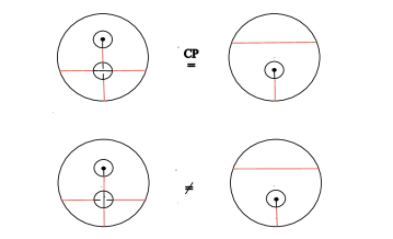
Figure 5. The additional relations on $\mathsf{wF}$; note the asymmetry of the CP relation.

As with $w$-tangles, $\mathsf{wF}$ is a discrete circuit algebra where elements of the set $\mathsf{\mathsf{wF}}[L^{-}_{i};L^{+}_{i}]$ are $w$-foams. Notice that in $\mathsf{wF}$ the cardinality of $L^{-}_{i}$ may not be the same as $L^{+}_{i}$, as vertices allow for strands to merge and split. An example of a $w$-foam is presented on the left in Figure 7.

The auxiliary operations on $\mathsf{wF}$ are external to the structure of a circuit algebra, which is to say that these are operations that are not parametrised by the operad of wiring diagrams. The full topological explanation of these operations can be found in [BND17, Section 4.1.3].

Definition 2.15.

The circuit algebra $\mathsf{wF}$ is equipped with the following auxiliary operations:

1. Orientation switch $S_{e}$: Diagrammatically, orientation switch reverses the direction of the strand $e$. Topologically, this operation switches both the 1D direction and the 2D orientation of the tube of the strand $e$.

2. Adjoint $A_{e}$: Diagrammatically, the adjoint operation reverses the direction of the strand $e$ and conjugates each crossing $e$ passes over by virtual crossings. Topologically, it reverses only the 1D direction of a tube $e$, but not the 2D orientation of the surface.

3. Unzip, and disc unzip $u_{e}$: Diagrammatically, unzip doubles the strand $e$ between two foam vertices using the blackboard framing, then attaches the ends of the doubled strands to the corresponding ends from the foam vertices, as in Figure 6. A similar operation for capped strands is disc unzip, also illustrated in Figure 6. Topologically, this operation doubles a tube in the framing direction.

4. Deletion $d_{e}$: It deletes the strand $e$, as long as $e$ is not attached to foam vertices on either end (these are called “long strands”).

The circuit algebra of $w$-foams is an example of a circuit algebra with a skeleton. In the context of Remark 2.9, a circuit algebra with a skeleton is a wheeled prop for which the set of objects also forms a wheeled prop.

Definition 2.16.

The circuit algebra of $w$-foam skeleta

$$\mathcal{S}=\mathsf{CA}\left<\upcap,\includegraphics[width=14.45377pt]{Vertex.pdf}\right>$$

is the free circuit algebra generated by the oriented caps and vertices . Moreover, this circuit algebra also possesses auxiliary operations: $S_{e},A_{e},u_{e}$ and $d_{e}$.

Figure 6. The unzip operation doubles a tube edge ending in the distinguished edges of two foamed vertices. Disc unzip doubles a capped strand which ends as a distinguished strand of a vertex.

An example of an element of $\mathcal{S}$ is depicted on the right in Figure 7. We saw in Example 2.8 that since $\mathcal{S}$ is a free circuit algebra, it contains every element of $\mathsf{WD}(L^{\pm}_{0};-)$. In particular, $\mathcal{S}$ contains all of the symmetric groups. As with $w$-tangles, we can project the circuit algebra of $w$-foams to the underlying circuit algebra of skeleta:

Definition 2.17.

For any pair of label sets $L^{-},L^{+}$ we define a skeleton projection map

which “flattens” the generators and to . We write $\mathsf{wF}(s)=\pi^{-1}(s)$ for the subset of foams $\mathsf{wF}[L^{-};L^{+}]$ with skeleton $s\in\mathcal{S}$.

Example 2.18.

In Figure 7, the circle on the left depicts a $w$-foam as an element of the circuit algebra $\mathsf{wF}$, given as a wiring diagram composition $\mathfrak{D}(\undercrossing,\includegraphics[width=14.45377pt]{Vertex.pdf})$. The black circles represent the input discs of the wiring diagram $\mathfrak{D}$, in which we have drawn the generators and . These generators are composed via the (abstract) $1$-manifold in $\mathfrak{D}$, which is depicted in red. The picture on the right of Figure 7 is the projection of this foam onto its skeleton, which is an element of the circuit algebra $\mathcal{S}$. The generator is sent to in the skeleton, which forms part of the wiring diagram.

Figure 7. A projection of a $w$-foam to its skeleton.

Proposition 2.19.

The skeleton projection maps assemble to give a homomorphism of circuit algebras, meaning that the following diagram commutes for all wiring diagrams $\mathfrak{D}$:

Skeleton projections also commute with all auxiliary operations.

Proof.

To verify this, observe that since the map $\pi$ is defined on generators, it is a circuit algebra map if it respects the relations of $\mathsf{wF}$. As one example, consider the relation R$2$ (Figure 3). The projection $\pi$ sends both sides of R$2$ to the identity element in the symmetric group $\mathcal{S}_{2}$ and thus $\pi$ preserves the relation R$2$. The remainder of the relations are equally straightforward, and so is the commutativity with auxiliary operations. We leave these to the reader to check. ∎

As the projection map is a homomorphism of circuit algebras, it follows that we can use the skeleton to provide an indexing of the circuit algebra of $w$-foams and write

$$\mathsf{wF}:=\coprod_{s\in\mathcal{S}}\mathsf{wF}(s).$$

Note, however, that for a specific $s\in\mathcal{S}$ the set $\mathsf{wF}(s)$ is not a circuit subalgebra of $\mathsf{wF}$.

2.3. Completion of $\mathbf{w}$-foams

In this section, we construct a prounipotent completion of the circuit algebra $\mathsf{wF}$. This is largely formal: circuit algebras are algebras over the operad of wiring diagrams (Definition 2.3) and thus completion of a circuit algebra is the completion of an algebra over an operad similar to that in [Fre98, 1.4.2]. The main difference between this section and [Fre98, 1.4.2] is that we index the circuit algebra $\mathsf{wF}$ by skeleta as opposed to the arity of the operations.

Definition 2.20.

An ideal $\mathcal{I}$ of a linear circuit algebra $\mathsf{V}=\{\mathsf{V}[L^{-};L^{+}]\}$ is a collection

$$\mathcal{I}=\{\mathcal{I}[L^{-};L^{+}]\subseteq\mathsf{V}[L^{-};L^{+}]\}\quad\text{where}$$

$$\mathfrak{D}(p_{1},\ldots,p_{r},k)\in\mathcal{I}[L_{0}^{+};L_{0}^{-}]\quad\text{whenever}\quad p_{i}\in\mathsf{V}[L_{i}^{-};L_{i}^{+}],1\leq i\leq r,\quad\text{and}\quad k\in\mathcal{I}[L_{j}^{-};L_{j}^{+}].$$

Equivalently, $\mathcal{I}$ is an ideal if the action of the operad $\mathsf{WD}$ descends to a circuit algebra structure on the quotient $\mathsf{V}/\mathcal{I}$.

The $n$th power ideal $\mathcal{I}^{n}$ consists of operations $\mathfrak{D}(p_{1},\ldots,p_{r})$ in which at least $n$ of the $p_{i}$, $1\leq i\leq r$, are in $\mathcal{I}$.

A quotient circuit algebra $\mathsf{V}/\mathcal{I}^{n}$ is said to be nilpotent if the circuit algebra multiplications

vanish for all wiring diagrams $\mathfrak{D}$ with $r>R$ input discs, for some $R$.

Definition 2.21.

A circuit algebra $\mathsf{V}$ is complete if $\mathsf{V}=\lim_{n}\mathsf{V}/\mathcal{I}^{n}$, where $\mathcal{I}^{n}$, $n\geq 1$ is a descending sequence of ideals of $\mathsf{V}$ and each $\mathsf{V}/\mathcal{I}^{n}$ is nilpotent.

To complete the circuit algebra $\mathsf{wF}$, we first linearly extend $\mathsf{wF}$ to a circuit algebra in $\mathbb{Q}$-vector spaces. For each skeleton $s\in\mathcal{S}$, let $\mathbb{Q}[\mathsf{wF}](s)$ denote the $\mathbb{Q}$-vector space of formal linear combinations of $w$-foams $T_{i}$ with skeleton $s\in\mathcal{S}$,

$$\sum_{T_{i}\in\mathsf{wF}(s)}\alpha_{i}T_{i}\in\mathbb{Q}[\mathsf{wF}](s).$$

The collection of vector spaces

$$\mathbb{Q}[\mathsf{wF}]=\bigsqcup_{s\in\mathcal{S}}\mathbb{Q}[\mathsf{wF}](s)$$

forms a circuit algebra where the operad of wiring diagrams acts by the linear extension of the action on $\mathsf{wF}$. In particular, $\mathbb{Q}[\mathsf{wF}]$ is a linear circuit algebra with skeleton $\mathcal{S}$.

Definition 2.22.

At each skeleton $s\in\mathcal{S}$ we define an augmentation map

$$\epsilon_{s}:\mathbb{Q}[\mathsf{wF}](s)\ \longrightarrow\ \mathbb{Q}$$

$$\Sigma\alpha_{i}T_{i}\mapsto\Sigma\alpha_{i}.$$

We denote the kernel of $\epsilon_{s}$ by $\mathcal{I}(s)$. The augmentation ideal of $\mathbb{Q}[\mathsf{wF}]$ is the disjoint union

$$\mathcal{I}=\bigsqcup_{s\in\mathcal{S}}\mathcal{I}(s).$$

Lemma 2.23.

$\mathcal{I}$ is an ideal in $\mathbb{Q}[\mathsf{wF}]$.

Proof.

Let $\mathfrak{D}$ be a wiring diagram composing the elements $p_{1},...,p_{r},k$, where $p_{i}\in\mathbb{Q}[\mathsf{wF}](s_{i})$, $1\leq i\leq r$, and $k\in\mathcal{I}(s_{k})$. We then verify that the composite $\mathfrak{D}(p_{1},\ldots,p_{r},k)$ is in $\mathcal{I}$.

Because a circuit algebra is an algebra over an operad, circuit algebra composition is associative and equivariant. It follows that any circuit algebra composition $\mathfrak{D}(p_{1},\ldots,p_{r},k)$ can be equivalently written $\mathfrak{D}_{1}(\mathfrak{D}_{2}(p_{1},\ldots p_{r-1},k),p_{r}).$ Therefore, without loss of generality we may assume that $\mathfrak{D}$ has only two inputs.

Given elements $p\in\mathbb{Q}[\mathsf{wF}](s)$ and $k\in\mathcal{I}(s_{k})$ with

$$p=\sum_{j}\alpha_{j}T_{j}\quad\text{and}\quad k=\sum_{i}\lambda_{i}K_{i},\quad\text{ with }T_{j}\in\mathsf{wF}(s),\text{ and }K_{i}\in\mathsf{wF}(s_{k}),$$

the composite via the wiring diagram $\mathfrak{D}$ is by definition

$$\mathfrak{D}(p,k)=\sum_{j}\alpha_{j}\sum_{i}\lambda_{i}\;\;\mathfrak{D}(T_{j},K_{i}).$$

Since $k$ is in $\mathcal{I}(s_{k})$ we know that $\sum_{i}\lambda_{i}=0$. It follows that $\sum_{j}\alpha_{j}\sum_{i}\lambda_{i}=0$ and therefore the composition $\mathfrak{D}(p,k)$ is in $\mathcal{I}$. The lemma now follows. ∎

Since $\mathcal{I}$ is an ideal, $\mathbb{Q}[\mathsf{wF}]/\mathcal{I}$ is a circuit algebra. The next lemma implies that the auxiliary operations are also well-defined on the quotient:

Lemma 2.24.

For any $k\in\mathcal{I}$, the w-foams resulting from auxiliary operations $u_{e}(k)$, $S_{e}(k)$, $A_{e}(k)$ and $d_{e}(k)$ are in $\mathcal{I}$ whenever these operations are defined.

Proof.

Let $p\in\mathbb{Q}[\mathsf{wF}](s)$ be an element with $p=\sum_{T_{j}\in\mathsf{wF}(s)}\alpha_{j}T_{j}$. For a strand $e$ in the skeleton $s\in\mathcal{S}$, the unzip operation produces $u_{e}(p)\in\mathbb{Q}[\mathsf{wF}](u_{e}(s))$, which is by definition the element

$$u_{e}(p)=\sum_{u_{e}(T_{j})\in\mathsf{wF}(u_{e}(s))}\alpha_{j}u_{e}(T_{j}).$$

In this case, the coefficients remain unchanged, so if $\sum_{T_{j}}\alpha_{j}=0$ and $p\in\mathcal{I}$, this still holds for $u_{e}(p)$. The same argument works for the operations $S_{e}$, $A_{e}$ and $d_{e}$. ∎

For each $s\in\mathcal{S}$, the $\mathbb{Q}$-vector space $\mathbb{Q}[\mathsf{wF}](s)$ admits a descending filtration given by powers of the augmentation ideal:

$$\mathbb{Q}[\mathsf{wF}](s)\supset\mathcal{I}(s)\supset\mathcal{I}^{2}(s)\supset\ldots\supset\mathcal{I}^{n}(s)\supset\ldots.$$

Since circuit algebra composition and the auxiliary operations are compatible with this filtration, $\mathbb{Q}[\mathsf{wF}]$ is a circuit algebra in filtered $\mathbb{Q}$-vector spaces.

Definition 2.25.

The (prounipotent) completion of the $\mathbb{Q}$-vector space $\mathbb{Q}[\mathsf{wF}](s)$ is the inverse limit of the system

$$\mathbb{Q}[\mathsf{wF}](s)/\mathcal{I}(s)\stackrel{{\scriptstyle}}{{\leftarrow}}\mathbb{Q}[\mathsf{wF}](s)/\mathcal{I}^{2}(s)\stackrel{{\scriptstyle}}{{\leftarrow}}\mathbb{Q}[\mathsf{wF}](s)/\mathcal{I}^{3}(s)\stackrel{{\scriptstyle}}{{\leftarrow}}...$$

We denote the resulting completed $\mathbb{Q}$-vector space by $\widehat{\mathsf{wF}}(s)=\lim_{n}\mathbb{Q}[\mathsf{wF}](s)/\mathcal{I}^{n}(s)$.

The passage from filtered $\mathbb{Q}$-vector spaces to completed $\mathbb{Q}$-vector spaces extends to a lax symmetric monoidal functor ([Fre17a, Proposition 7.3.11; Section 7.3.12])

Algebras over coloured operads transfer over symmetric monoidal functors, which in this case means that, for every wiring diagram $\mathfrak{D}$, the following diagram commutes:

The following proposition follows immediately.

Proposition 2.26.

The completion of $w$-foams

$$\widehat{\mathsf{wF}}:=\coprod_{s\in\mathcal{S}}\widehat{\mathsf{wF}}(s)$$

is a circuit algebra with auxiliary operations $A_{e}$, $S_{e}$, $u_{e}$ and $d_{e}$. ∎

Definition 2.27.

For every skeleton $s\in\mathcal{S}$, the filtration of $\mathbb{Q}[\mathsf{wF}](s)$ by powers of the augmentation ideal gives rise to the (complete) associated graded vector space

$$\mathsf{A}(s)=\prod_{n\geq 0}\mathcal{I}^{n}(s)/\mathcal{I}^{n+1}(s).$$

The functor from filtered $\mathbb{Q}$-vector spaces to completed $\mathbb{Q}$-vector spaces restricts to a lax symmetric monoidal functor from filtered $\mathbb{Q}$-vector spaces to graded $\mathbb{Q}$-vector spaces [Fre17a, Lemma 7.3.10; Section 7.3.13]. It follows from the same argument as above that the graded $\mathbb{Q}$-vector spaces $\mathsf{A}(s)$ assemble into a circuit algebra

$$\mathsf{A}:=\coprod_{s\in\mathcal{S}}\mathsf{A}(s).$$

Moreover, the filtration is compatible with the auxiliary operations of $\mathsf{wF}$, and therefore $\mathsf{A}$ is a circuit algebra with the associated graded auxiliary operations, also denoted $A_{e}$, $S_{e}$, $u_{e}$ and $d_{e}$. The following proposition shows that completion of the circuit algebra $\mathsf{wF}$ is filtration-preserving and that $\mathsf{A}$ is the associated graded space of $\widehat{\mathsf{wF}}$ also.

Proposition 2.28.

The circuit algebra $\widehat{\mathsf{wF}}$ is filtered by $\widehat{\mathcal{I}^{n}}:=\displaystyle{\lim_{k>n}\mathcal{I}^{n}/\mathcal{I}^{k}}$. Moreover, with this filtration it is a complete circuit algebra and there is a canonical isomorphism of circuit algebras $\text{gr}(\widehat{\mathsf{wF}})\cong\mathsf{A}$.

Proof.

Our first goal is to show that $\widehat{\mathsf{wF}}$ is filtered. We know that the $\mathbb{Q}$-module $\mathbb{Q}[\mathsf{wF}](s)$ has a filtration by powers of the augmentation ideal and that the quotient maps $\mathbb{Q}[\mathsf{wF}](s)\rightarrow\mathbb{Q}[\mathsf{wF}](s)/\mathcal{I}^{\ell}(s)$ lifts canonically to a morphism

$$\mathbb{Q}[\mathsf{wF}](s)\rightarrow\widehat{\mathsf{wF}}(s)=\lim_{n}\mathbb{Q}[\mathsf{wF}](s)/\mathcal{I}^{n}(s).$$

This induces a canonical filtration on $\widehat{\mathsf{wF}}(s)$ with $F_{\ell}(\widehat{\mathsf{wF}}(s))=\text{ker}\left(\widehat{\mathsf{wF}}(s)\rightarrow\mathbb{Q}[\mathsf{wF}](s)/\mathcal{I}^{\ell+1}(s)\right)$ which are the kernels of the projection of maps on the right-hand tower

$$\leavevmode\hbox to204.81pt{\vbox to55.29pt{\text{[drawing]}}}. {F_{\ell}(\widehat{\mathsf{wF}}(s))} {\widehat{\mathsf{wF}}(s)} {\mathbb{Q}[\mathsf{wF}](s)/\mathcal{I}^{\ell+1}(s)} {F_{\ell-1}(\widehat{\mathsf{wF}}(s))} {\widehat{\mathsf{wF}}(s)} {\mathbb{Q}[\mathsf{wF}](s)/\mathcal{I}^{\ell}(s)} \scriptstyle{\subseteq} \scriptstyle{=} {F_{\ell}(\widehat{\mathsf{wF}}(s))} {\widehat{\mathsf{wF}}(s)} {\mathbb{Q}[\mathsf{wF}](s)/\mathcal{I}^{\ell+1}(s)} {F_{\ell-1}(\widehat{\mathsf{wF}}(s))} {\widehat{\mathsf{wF}}(s)} {\mathbb{Q}[\mathsf{wF}](s)/\mathcal{I}^{\ell}(s)} \scriptstyle{\subseteq} \scriptstyle{=}$$

What is more, we have $F_{\ell}(\widehat{\mathsf{wF}}(s))=\widehat{\mathcal{I}}^{\ell}(s)=\displaystyle{\lim_{k>\ell}\mathcal{I}(s)^{\ell}/\mathcal{I}(s)^{k}}$ by [Fre17a, 7.3.6] and

$$F_{\ell}(\widehat{\mathsf{wF}}(s))/F_{\ell+1}(\widehat{\mathsf{wF}}(s))\cong\mathcal{I}^{\ell}(s)/\mathcal{I}^{\ell+1}(s).$$

In a similar fashion, we define the associated graded as

$$\mathsf{A}^{\ell}(s)=\text{ker}\left(\mathbb{Q}[\mathsf{wF}](s)/\mathcal{I}^{\ell+1}(s)\twoheadrightarrow\mathbb{Q}[\mathsf{wF}](s)/\mathcal{I}^{\ell}(s)\right).$$

By a short calculation, each component of the associated graded $\mathsf{A}$ is identified as

$$\mathsf{A}^{\ell}(s)=\mathcal{I}^{\ell}(s)/\mathcal{I}^{\ell+1}(s)\cong\widehat{\mathcal{I}}^{\ell}(s)/\widehat{\mathcal{I}}^{\ell+1}(s)=\text{gr}(\widehat{\mathsf{wF}}(s))^{\ell}.$$

These filtrations respect the symmetric monoidal structure of filtered $\mathbb{Q}$-modules [Fre17a, 7.3.10] and thus we can lift this identification to a canonical isomorphism of circuit algebras $\text{gr}(\widehat{\mathsf{wF}})\cong\mathsf{A}$ . ∎

3. Arrow diagrams and the Kashiwara–Vergne Lie algebras

3.1. The circuit algebra of arrow diagrams

Variants of chord diagram spaces – chord diagrams, Jacobi diagrams, arrow diagrams – are prevalent throughout knot theory, and in particular, the theory of finite type invariants. They are combinatorial models for the associated graded spaces of filtered linearised spaces of knots, braids, or other knotted objects. Chord diagram spaces also arise in quantum algebra as a computational tool capturing properties of Lie algebras.

Informally, a Jacobi diagram is a graph with trivalent and univalent vertices, whose univalent vertices are arranged on a knot or tangle skeleton (e.g. a circle, or $n$ disjoint horizontal lines). These diagrams are considered modulo a set of relations: STU, IHX and anti-symmetry, and others depending on the context. The trivalent vertex captures the algebraic properties of a Lie bracket, for example, the IHX relation corresponds to the Jacobi identity. For more details on Jacobi diagrams in the classical setting see, for example, [BN95] or [CDM12, Chapter 5] and references therein.

The space of $w$-Jacobi diagrams is an oriented variant of Jacobi diagrams, on $w$-foam skeleta, which gives a combinatorial description for the associated graded space of $w$-foams. They are introduced and studied in [BND17, Definition 3.8 and Section 4.2]. Here, we briefly review their definition and most important properties.

Definition 3.1.

A $w$-Jacobi diagram on a $w$-foam skeleton $s\in\mathcal{S}$ is a – possibly infinite – linear combination of uni-trivalent oriented graphs with the following properties:

1. trivalent vertices are incident to two incoming edges and one outgoing edge, and are cyclically ordered

2. univalent vertices are attached to $s$ (this data is combinatorial, i.e. only the ordering of univalent vertices along each skeleton edge matters).

The collection of $w$-Jacobi diagrams on a given $s\in\mathcal{S}$ forms a graded complete vector space, where the degree is given by half the number of vertices in a diagram (including trivalent and univalent vertices).

An example of a $w$-Jacobi diagram is depicted in Figure 8 where the oriented graph is depicted in red and the $w$-foamed skeleton is in black.

Figure 8. On the left is an example of a $w$-Jacobi diagram. Sometimes, we denote an arbitrary w-Jacobi diagram located on a certain part of a skeleton by a red box, as shown on the right.

Definition 3.2.

Given a $w$-foam skeleton $s\in\mathcal{S}$, let $\mathsf{J}(s)$ denote the graded complete $\mathbb{Q}$-vector space of $w$-Jacobi diagrams on the skeleton $s$, modulo the STU, AS, IHX, TC, VI, CP and RI relations shown in Figures 9 and 10 and briefly explained below.

The convention for diagrammatic relations is that only the relevant part of the diagrams is depicted, and the rest of the diagrams is arbitrary, but the same throughout the relation. Importantly, the TC relation states that arrow Tails Commute along skeleton strands. The CP relation means that any arrow diagram with an arrow head immediately adjacent to a cap is zero. The VI relation states that an arrow diagram with a single arrow ending (head or tail) on the distinguished edge of a skeleton vertex is equivalent to the sum of the two arrow diagrams with the arrow ending on each of the two merging strands. This version of the VI relation applies when the non-distinguished strands of the skeleton vertex are both incoming or both outgoing. If their orientations are opposite, a sign is introduced. Note that the VI relation implies that an arrow diagram with $k$ arrows ending (heads or tails) on the distinguished edge of a skeleton vertex is equal to a sum of $2^{k}$ arrow diagrams where the arrow endings are split between the two non-distinguished edges in all possible ways.

Figure 9. The STU, TC, AS and IHX relations.

Figure 10. Relations VI, CP and RI in $\mathsf{A}$.

All of these relations are degree-preserving and hence the quotient $\mathsf{J}(s)$ remains graded. The STU and TC relations in fact imply the AS and IHX relations; the latter are stated for convenience. We remark that the arrow diagram relations described arise from the relations of $\mathsf{wF}$ via the associated graded construction. For a brief explanation of this point, see [BND17, Definition 3.8 and Proposition 3.9].

The collection $\mathsf{J}=\{\mathsf{J}(s)\}_{s\in\mathcal{S}}$ assembles naturally into a linear circuit algebra where the operad of wiring diagrams acts on $\mathsf{J}$ by wiring together the skeleta and preserving the arrow graphs.

The circuit algebra $\mathsf{J}$ admits a – not obvious – finite presentation. Note that via iterated applications of the STU relations, all trivalent vertices in Jacobi diagrams can be eliminated. In other words, all Jacobi diagrams are equivalent to an “arrows only” form: a linear combination of diagrams in which only oriented arrows are attached to the foam skeleton. Such diagrams are called arrow diagrams, as below. It turns out that the arrow diagram equivalent of a $w$-Jacobi diagram is unique up to the arrow diagram relations 4T, TC, VI, CP and RI, and this leads to an isomorphic finite presentation of $\mathsf{J}$ as a circuit algebra, denoted $\mathsf{A}$, as below. [BND17, Theorem 4.6, based on Theorem 3.13]

Definition 3.3.

[BND17, Definition 4.8] The circuit algebra of arrow diagrams is the complete circuit algebra in $\mathbb{Q}$-vector spaces with presentation

$$\mathsf{A}:=\mathsf{CA}\left<\rightarrowdiagram,\upcap,\includegraphics[width=14.45377pt]{Vertex.pdf}\mid\text{4T, TC, VI, CP, RI}\right>.$$

In addition, $\mathsf{A}$ is equipped with the associated graded auxiliary operations: orientation switches $S_{e},A_{e}$, unzips $u_{e}$, and strand deletion $d_{e}$ described in Definition 3.6.

The relations are shown in Figures 10 and 11. There is a well-defined skeleton map $\pi:\mathsf{A}\rightarrow\mathcal{S}$ which forgets arrows, so $\mathsf{A}$ is indexed by skeleta: $\mathsf{A}=\coprod_{s\in\mathcal{S}}\mathsf{A}(s)$, where $\mathsf{A}(s):=\pi^{-1}(s)$. For any given $s\in S$, $\mathsf{A}(s)$ is a graded complete vector space, where the degree is given by the number of arrows.

Figure 11. Relation $4$T in $\mathsf{A}$.

The following is Theorem 4.5 of [BND17]. In the theory of finite type invariants, this is called a “bracket rise” theorem, and the proof uses standard Jacobi diagram techniques, as in [CDM12, Chapter 5], for example. We give a proof sketch below to illustrate the main points.

Theorem 3.4.

There is a canonical isomorphism of circuit algebras $\mathsf{A}\cong\mathsf{J}$.

Proof.

(Sketch) Since arrow diagrams are in particular $w$-Jacobi diagrams (without trivalent vertices), there is a natural inclusion $\iota_{s}:\mathsf{A}(s)\rightarrow\mathsf{J}(s)$. The image of the $4T$ relation under $\iota_{s}$ vanishes by the STU relation. The rest of the relations of $\mathsf{A}(s)$ are also imposed in $\mathsf{J}(s)$, so $\iota_{s}$ is well-defined. The inclusion $\iota_{s}$ has an inverse $\phi_{s}:\mathsf{J}(s)\rightarrow\mathsf{A}(s)$ which resolves all of the trivalent vertices of a $w$-Jacobi diagram by repeated applications of the STU relation, as mentioned above; to show that this is well-defined is a case analysis.

The operad $\mathsf{WD}$ acts on both $\mathsf{J}$ and $\mathsf{A}$ by wiring together skeleta and preserving arrows or arrow graphs. Thus, the collection of all isomorphisms $\iota_{s}:\mathsf{A}(s)\rightarrow\mathsf{J}(s)$ assembles into a circuit algebra isomorphism $\iota:\mathsf{A}\rightarrow\mathsf{J}$. ∎

Remark 3.5.

The presentation $\mathsf{A}$ has the obvious advantages of a finite presentation; while the definition of $\mathsf{J}$ has a more convenient set of relations, especially in the context of Lie algebras, which plays a prominent role later in this paper. Given the canonical isomorphism $\mathsf{A}\cong\mathsf{J}$, from now on we do not distinguish $w$-Jacobi and arrow diagrams, refer to both as “arrow diagrams”, and use $\mathsf{A}$ to denote either space. In general, we work with Jacobi diagrams, but we use the finite presentation of $\mathsf{A}$ in a fundamental way in Sections 4 and 5.

The circuit algebra $\mathsf{A}$ is equipped with auxiliary operations: $S_{e},A_{e},u_{e}$ and $d_{e}$, which are the associated graded operations of the $w$-foam operations by the same name described in Definition 2.15.

Definition 3.6.

Let $e$ denote a strand (edge) in the skeleton $s\in\mathcal{S}$. The auxiliary operations on $\mathsf{A}$ are defined as follows:

1. The orientation switch $S_{e}:\mathsf{A}(s)\rightarrow\mathsf{A}(S_{e}(s))$ reverses the direction of $e$ and multiplies each arrow diagram by

   $$(-1)^{\#(\text{arrow heads and tails on }e)}.$$

2. The adjoint map $A_{e}:\mathsf{A}(s)\rightarrow\mathsf{A}(A_{e}(s))$ reverses the direction of $e$ and multiplies each arrow diagram by

   $$(-1)^{\#(\text{arrow heads on }e)}.$$

3. The unzip and disc unzip maps, both denoted $u_{e}:\mathsf{A}(s)\rightarrow\mathsf{A}(u_{e}(s))$, unzip the strand $e$ and map each arrow ending on $e$ to a sum of two arrows, as shown in Figure 12.

4. The deletion map $d_{e}:\mathsf{A}(s)\rightarrow\mathsf{A}(d_{e}(s))$ deletes the long strand $e$ (which is not incident to any skeleton vertices), and an arrow diagram with any arrow head or tail on $e$ is sent to 0.

Figure 12. The unzip operations $u_{e}$ for arrow diagrams. A single arrow ending on $e$ is mapped to a sum of two arrows. If a diagram has $k$ arrows ending on $e$, it is mapped to a sum of $2^{k}$ terms.

Remark 3.7.

The operations are well-defined, that is, they commute with all the relations on $\mathsf{A}$. For example, the commutative diagram in Figure 13 shows how unzip and the “vertex invariance” operation (VI) are compatible. The reader may verify as an exercise that all of the operations are compatible with the relations on $\mathsf{A}$.

Figure 13. The compatibility of the unzip operation with the VI relation.

Remark 3.8.

We note that the rotation invariance $RI$ relation of $\mathsf{A}$ has an equivalent “wheel” formulation for Jacobi diagrams, as shown in Figure 14.

Figure 14. The RI relation, reformulated.

Recall that the complete associated graded space of $\mathsf{wF}$ (Definition 2.27) was also denoted $\mathsf{A}$, like the circuit algebra of arrow diagrams. This is no accident, as the two spaces are canonically isomorphic. This follows from the existence of a homomorphic expansion for $\mathsf{wF}$ combined with [BND17] Propositions 3.9 and 2.7:

Theorem 3.9.

[BND17] The circuit algebra $\mathsf{A}$ of arrow diagrams is canonically isomorphic to the complete associated graded circuit algebra of $\mathsf{wF}$ and the diagrammatic operations $S_{e},A_{e},u_{e}$ and $d_{e}$ are the associated graded maps of their topological counterparts.

3.2. Algebraic structures in $\mathsf{A}$

At each $w$-foam skeleton $s\in\mathcal{S}$, the $\mathbb{Q}$-vector space $\mathsf{A}(s)$ can be equipped with a counital, coassociative coproduct:

Definition 3.10.

For each $s\in\mathcal{S}$ the coproduct

sends an arrow diagram $D\in\mathsf{A}(s)$ to the sum of all ways of distributing the connected components of the arrow graph of $D$ – that is, the diagram minus the skeleton – amongst two copies of the skeleton.

An example of the coproduct is given in Figure 15. Note that the relative position of the two connected components of the Jacobi diagram is preserved.

Figure 15. The coproduct of an arrow diagram in $\mathsf{A}(\uparrow_{3})$. The arrow diagram on the left has two connected components (after the skeleton is removed). Hence, the coproduct is a sum of four terms.

It is a straightforward exercise, which we leave to the reader, to verify that the coproduct in Definition 3.10 is counital and coassociative.

Definition 3.11.

An arrow diagram $D\in\mathsf{A}(s)$ is said to be primitive if

$$\Delta(D)=D\otimes 1+1\otimes D.$$

A quick inspection shows that primitive arrow diagrams are (linear combinations of) diagrams whose arrow graph (the arrow diagram with the skeleton removed) is connected. For example, the arrow diagram in Figure 15 is not primitive, but the arrow diagram in Figure 19 is primitive.

In [BND17, Section 3.2] there is a full characterisation of connected arrow graphs in terms of trees and wheels:

1. trees are cycle-free arrow graphs oriented towards a single head, and

2. wheels consist of an oriented cycle with inward-oriented arrow “spokes”.

The two components of the arrow graph in Figure 15 are a tree and a 2-wheel. Arrow graphs where trees are attached to a cycle can be resolved using IHX relations to a linear combination of wheels. Arrow graphs with more than one cycle are zero as they cannot satisfy the two-in-one-out condition at all vertices.

An important case of arrow diagram spaces are arrow diagrams on a skeleton which consists of $n$ long strands, drawn as $n$ upward-oriented vertical lines, $\mathsf{A}(\uparrow_{n})$. For example, the arrow diagrams in Figure 15 are in $\mathsf{A}(\uparrow_{3})$. In addition to the coalgebra structure, $\mathsf{A}(\uparrow_{n})$ is equipped with an associative product

given by “stacking”. Stacking is a circuit algebra operation realised by the wiring diagram in Figure 16. This product is associative because wiring diagram composition is associative. The multiplicative unit is the empty arrow diagram (with no arrows) in $\mathsf{A}(\uparrow_{n})$.

Figure 16. The wiring diagram $\mathfrak{D}_{s}$ for stacking elements of $\mathsf{A}(\uparrow_{n})$.

The following fact is established in [BND17, Section 3.2]:

Proposition 3.12.

The stacking product and arrow diagram coproduct make $\mathsf{A}(\uparrow_{n})$ into a Hopf algebra, and, by the Milnor–Moore theorem [MM65], $\mathsf{A}(\uparrow_{n})$ is isomorphic to the completed universal enveloping algebra over its primitive elements.

Note that arrow diagrams on an arbitrary skeleton do not assemble into a Hopf algebra. However, the following lemma is a straightforward application of the VI relation:

Lemma 3.13.

[BND17, Lemma 4.7] There is a canonical isomorphism of vector spaces

$$\mathsf{A}(\includegraphics[width=14.45377pt]{Vertex.pdf})\cong\mathsf{A}(\uparrow_{2}).$$

Therefore, the Hopf algebra structure on $\mathsf{A}(\uparrow_{2})$ can be pulled back along this isomorphism to give a Hopf algebra structure on $\mathsf{A}(\includegraphics[width=14.45377pt]{Vertex.pdf}).$

Example 3.14.

The product of two arrow diagrams $A$ and $B$ in $\mathsf{A}(\includegraphics[width=14.45377pt]{Vertex.pdf})$ can be realised by a sequence of circuit algebra compositions and unzip, as shown in Figure 17. First compose $A$ with a vertex of the opposite orientation, and compose with $B$ (circuit algebra operations). Then unzip the middle edge. This product, together with the coproduct of Definition 3.10 makes $\mathsf{A}(\includegraphics[width=14.45377pt]{Vertex.pdf})$ into a Hopf algebra.

Figure 17. Stacking multiplication realised on a vertex.

3.3. The Kashiwara–Vergne spaces

In this section, we review the relationship between the circuit algebra of arrow diagrams and the spaces where the Kashiwara–Vergne equations “live”, based on [BND17, Section 3.2] and [AT12].

Throughout, we will write $\widehat{\mathfrak{lie}}_{n}$ for the degree completed free Lie algebra generated by $x_{1},\ldots,x_{n}$. In the case of $n=1,2,3$ we will often write the generators as $x,y,z$ to reduce notational clutter. We let $\widehat{\mathfrak{ass}}_{n}:=\mathbb{Q}\left<\left<x_{1},\ldots,x_{n}\right>\right>$ denote the degree completed free associative algebra generated by the same symbols. As a completed Hopf algebra, $\widehat{\mathfrak{ass}}_{n}$ is the universal enveloping algebra of $\widehat{\mathfrak{lie}}_{n}$: $\widehat{U}(\widehat{\mathfrak{lie}}_{n})=\widehat{\mathfrak{ass}}_{n}.$ Degree completions throughout ensure that the group-like elements in $\widehat{U}(\widehat{\mathfrak{lie}}_{n})=\widehat{\mathfrak{ass}}_{n}$ are identified with the group $\exp(\widehat{\mathfrak{lie}}_{n})$.

A tangential derivation on $\widehat{\mathfrak{lie}}_{n}$ is a derivation $u$ of $\widehat{\mathfrak{lie}}_{n}$ which acts on the generators $x_{i}$ by $u(x_{i})=[x_{i},a_{i}]$, for some $a_{i}\in\widehat{\mathfrak{lie}}_{n}$. For this reason, we write tangential derivations as a tuple of Lie words $u:=(a_{1},\ldots,a_{n})$ ([AT12, Definition 3.2]). The collection of all tangential derivations of $\widehat{\mathfrak{lie}}_{n}$ forms a Lie algebra which we denote by $\mathfrak{tder}_{n}$, where the bracket $[u,v]$ is given by $[u,v](x_{k}):=u(v(x_{k}))-v(u(x_{k}))$; see [AT12, Proposition 3.4].

Example 3.15.

The tuple $t^{1,2}=(y,x)$ is a tangential derivation of $\widehat{\mathfrak{lie}}_{2}$, given by $t^{1,2}(x)=[x,y]$ and $t^{1,2}(y)=[y,x]$.

The tuple description of tangential derivations defines a map $(\widehat{\mathfrak{lie}}_{n})^{\oplus n}\to\mathfrak{tder}_{n}$, whose kernel is generated by the tuples $(0,...,0,x_{i},0,...,0)$, where $x_{i}$ appears in the $i$th component. Therefore, there is an isomorphism $(\widehat{\mathfrak{lie}}_{n})^{\oplus n}\cong\mathfrak{tder}_{n}\oplus\mathfrak{a}_{n}$, where $\mathfrak{a}_{n}$ is the $n$-dimensional abelian Lie algebra generated by $\{x_{1},...,x_{n}\}$.

Both $\widehat{\mathfrak{lie}}_{n}$ and $\widehat{\mathfrak{ass}}_{n}$ are naturally graded. Explicitly, $\widehat{\mathfrak{lie}}_{n}=\prod_{k\geq 1}\widehat{\mathfrak{lie}}_{n}^{k}$ where $\widehat{\mathfrak{lie}}_{n}^{k}$ is spanned by Lie words with $k$ letters. For example, $[x,z]\in\widehat{\mathfrak{lie}}_{3}^{2}$ and $[y,[x,z]]\in\widehat{\mathfrak{lie}}_{3}^{3}$. Similarly, $\widehat{\mathfrak{ass}}_{n}=\prod_{k\geq 1}\widehat{\mathfrak{ass}}_{n}^{k}$. This grading descends to the vector space of cyclic words.

Definition 3.16.

The complete graded vector space of cyclic words is the linear quotient

$$\mathrm{cyc}_{n}:=\widehat{\mathfrak{ass}}_{n}/\left<ab-ba\mid\forall a,b\in\widehat{\mathfrak{ass}}_{n}\right>=\widehat{\mathfrak{ass}}_{n}/[\widehat{\mathfrak{ass}}_{n},\widehat{\mathfrak{ass}}_{n}].$$

We denote the natural projection map by $\textrm{tr}:\widehat{\mathfrak{ass}}_{n}\rightarrow\mathrm{cyc}_{n}$.

The action of $\mathfrak{tder}_{n}$ on $\widehat{\mathfrak{lie}}_{n}$ extends to $\widehat{\mathfrak{ass}}_{n}$ by the Leibniz rule, and in turn descends to $\mathrm{cyc}_{n}$. We illustrate this in the following example, borrowed from [AT12, Example 3.18]:

Example 3.17.

Let $u=(y,0)\in\mathfrak{tder}_{2}$ and $a=\textrm{tr}(xy)\in\mathrm{cyc}^{2}_{2}$. Then

$$u\cdot a=\textrm{tr}(u(x)\,y+x\,u(y))=\textrm{tr}([x,y]y)=\textrm{tr}(xy^{2}-yxy)=0.$$

In [BND17, Section 3.2], primitive elements of $\mathsf{A}(\uparrow_{n})$ are mapped isomorphically to tangential derivations and cyclic words in the following way. Let $D$ be either a single tree or single wheel arrow graph on a skeleton of $n$ vertical strands. Label the skeleton strands with the generators $x_{1},x_{2},...,x_{n}$.

1. If $D$ is a tree, we construct an element of $(\widehat{\mathfrak{lie}}_{n})^{\oplus n}$. The tree determines a Lie word by reading the generator corresponding to the skeleton strand of each leaf (tail) of the tree, and combining these with brackets corresponding to each trivalent vertex; see Example 3.18 below. The placement of the root (head) of the tree determines which coordinate of $(\widehat{\mathfrak{lie}}_{n})^{\oplus n}$ the Lie word is placed in, as in the example.

2. If $D$ is a wheel, $D$ determines a cyclic word in the letters $x_{i}$, which is determined by the placement of the “spokes” of the wheel on the skeleton, and the orientation of the wheel.

Example 3.18.

Consider the element $t^{1,2}=(y,x)\in\mathfrak{tder}_{2}$ from Example 3.15. The arrow diagram corresponding to $t^{1,2}$ is depicted on the left in Figure 18. Similarly, the tree arrow diagram on the right of Figure 18 corresponds to $u=(0,[[x,y],z],0)\in\mathfrak{tder}_{3}$. The wheel in Figure 19 corresponds to the cyclic word $\textrm{tr}(x^{2}yz)\in\mathrm{cyc}_{3}^{4}$.

Figure 18. The arrow diagram on the left corresponds to $t^{1,2}=(y,x)\in\mathfrak{tder}_{2}$; the diagram on the right corresponds to $u=(0,[[x,y],z],0)\in\mathfrak{tder}_{3}$.

Figure 19. The cyclic word $\textrm{tr}(x^{2}yz)$ as an arrow diagram. We use the convention that wheels are oriented couterclockwise, unless otherwise marked.

The subspace of $\mathsf{A}(\uparrow_{n})$ spanned by primitive elements, $\mathsf{P}(\uparrow_{n})$, forms a Lie algebra with the bracket given by the algebra commutator of $\mathsf{A}(\uparrow_{n})$. There is a Lie algebra isomorphism $\mathsf{P}(\uparrow_{n})\cong(\mathfrak{tder}_{n}\oplus\mathfrak{a}_{n})\ltimes\mathrm{cyc}_{n}$ [BND17, Proposition 3.19]. In the semidirect product, $\mathfrak{a}_{n}$ is central and $\mathfrak{tder}_{n}$ acts on $\mathrm{cyc}_{n}$ as in Example 3.17, which in light of the discussion above can be realised in $\mathsf{A}(\uparrow_{n})$, as illustrated in Figure 20.

Figure 20. An illustration of the action of $\mathfrak{tder}_{n}$ on $\mathrm{cyc}_{n}$ from Example 3.17 realised as arrow diagrams.

Since, by the Milnor–Moore Theorem, $\mathsf{A}(\uparrow_{n})$ is the universal enveloping algebra of $\mathsf{P}(\uparrow_{n})$, this implies the following:

Proposition 3.19.

There is an isomorphism of Hopf algebras

$$\Upsilon:\mathsf{A}(\uparrow_{n})\stackrel{{\scriptstyle\cong}}{{\longrightarrow}}\widehat{U}((\mathfrak{tder}_{n}\oplus\mathfrak{a}_{n})\ltimes\mathrm{cyc}_{n}).$$

It is important to keep in mind that at the level of primitive elements $\Upsilon$ identifies $\mathfrak{tder}_{n}\oplus\mathfrak{a}_{n}$ with connected tree diagrams, and $\mathrm{cyc}_{n}$ with wheels.

Remark 3.20.

In [BND17, Proof of Proposition 19] the action of $\mathfrak{tder}_{n}$ on $\widehat{\mathfrak{lie}}_{n}$ is described in diagrammatic terms; we give a summary here. Let $D\in\mathsf{P}(\uparrow_{n})$ be an arrow diagram consisting of a single tree, corresponding to $u=(0,\ldots,a_{i},\ldots,0)\in\mathfrak{tder}_{n}$. The tails of $D$ correspond to the letters in the Lie word $a_{i}$ and the root of the tree (the single arrow head) is on the $i$th strand of $\mathsf{A}(\uparrow_{n})$.

We consider $D$ as an element of $\mathsf{A}(\uparrow_{n+1})$ by adding an empty skeletal strand to the right. The free Lie algebra $\widehat{\mathfrak{lie}}_{n}$ embeds in $\mathsf{A}(\uparrow_{n})$, by representing $x_{j}$ as an arrow from strand $j$ to the extra strand. Then $D$ acts on $x_{j}$ via the commutator, i.e. the difference of the stacking products $x_{j}D-Dx_{j}$. Using the TC and STU relations, one can verify that this commutator is in the image of $\widehat{\mathfrak{lie}}_{n}$.

We write $\operatorname{TAut}_{n}:=\exp(\mathfrak{tder}_{n})$ to denote the group associated to the Lie algebra $\mathfrak{tder}_{n}$. As a group, $\operatorname{TAut}_{n}$ consists of “basis-conjugating” automorphisms of $\exp(\widehat{\mathfrak{lie}}_{n})$: for any $e^{u}\in\operatorname{TAut}_{n}$ there exists an element $e^{a_{i}}\in\exp(\widehat{\mathfrak{lie}}_{n})$ where $e^{u}\cdot e^{x_{i}}=e^{-a_{i}}e^{x_{i}}e^{a_{i}}$.

After exponentiation, we obtain that the following diagram commutes:

(3.1)

Here, given $e^{u}\in\operatorname{TAut}_{n}$, by $\Upsilon^{-1}(u)$ we mean $\Upsilon^{-1}(((u+0),0))$ embedded on the first $n$ strands of $\mathsf{A}(\uparrow_{n})$. The map $\iota$ is the exponential of the embedding of $\widehat{\mathfrak{lie}}_{n}$ above. Ad denotes the adjoint action and “conj” denotes conjugation of the second component by the first.

Arrow diagrams with an arrow head adjacent to a cap vanish by the CP relation. Thus, when the skeleton consists only of capped strands, arrow heads can be eliminated entirely by successive applications of STU and CP relations. Arrow diagrams with no arrow heads can always be expressed as a linear combination of only wheels, which in turn can be encoded as cyclic words. This leads to the following lemma, which is a straightforward generalisation of [BND17, Lemma 4.6].

Lemma 3.21.

There is an isomorphism of graded vector spaces $\kappa:\mathsf{A}({}_{n})\stackrel{{\scriptstyle\cong}}{{\longrightarrow}}\mathrm{cyc}_{n}/\mathrm{cyc}_{n}^{1}$. Here $\mathrm{cyc}_{n}^{1}$ denotes the degree 1 component of cyclic words.

The reason for factoring out the degree $1$ component in this lemma is the $RI$ relation, see Figure 14.

Remark 3.22.

Note that cyclic words in one letter are power series, so we will also write $\kappa:\mathsf{A}({}_{1})\stackrel{{\scriptstyle\cong}}{{\longrightarrow}}\mathbb{Q}[[\xi]]/\langle\xi\rangle$, where the quotient is understood linearly. In addition, since $\mathrm{cyc}_{n}\cong\textrm{tr}(\mathbb{Q}\langle\langle x_{1},x_{2},...,x_{n}\rangle\rangle)$, we have, for example $\mathsf{A}({}_{2})\cong\textrm{tr}(\mathbb{Q}\langle\langle\xi,\zeta\rangle\rangle)/\langle\xi,\zeta\rangle$.

Remark 3.23.

The $\mathbb{Q}$-vector space $\mathsf{A}({}_{2})$ is a left $\mathsf{A}(\uparrow_{2})$-module with the action given by stacking:

$$\mathsf{A}(\uparrow_{2})\times\mathsf{A}({}_{2})\xrightarrow{\text{stack}}\mathsf{A}({}_{2}).$$

This stacking action is compatible with the natural action of $\mathfrak{tder}_{2}$ on $\mathrm{cyc}_{2}$ described in Example 3.17, in the sense that the following diagram commutes:

(3.2)

It is non-trivial to see why a stacking action agrees with a commutation action. In short, this is because $\mathfrak{tder}_{n}$ is embedded in $\mathsf{A}(\uparrow_{n})$ as trees, and the term of the commutator where the tree is adjacent to the cap vanishes by the CP relation. For a more thorough explanation, see [BND17, Remark 3.24].

The action of $\mathfrak{tder}_{n}$ on $\mathrm{cyc}_{n}$ can be formally exponentiated to a conjugation action of $\operatorname{TAut}_{n}$ on $\exp(\mathrm{cyc}_{n})$. This action commutes with the stacking action of $\mathsf{A}(\uparrow_{n})$ on $\mathsf{A}({}_{n})$ for the same reason as above:

(3.3)

3.3.1. Cosimplicial Structure

Tangential derivations admit a semi-cosimplicial structure, as described in [AT12, Section 3.2]. That is, for $i=0,1,...,n,$ there are Lie algebra homomorphisms, called coface maps $\delta_{i}:\mathfrak{tder}_{n-1}\rightarrow\mathfrak{tder}_{n}$ defined by sending the tangential derivation $u=(a_{1},\ldots,a_{n-1})$ to $\delta_{i}(u)=(a_{1},\ldots,0,\ldots,a_{n-1})$ in $\mathfrak{tder}_{n}$, where $0$ is inserted in the $i$th entry of $\delta_{i}(u)$, and the subsequent components are shifted.

To simplify notation, we will suppress the coface maps and use a superscript notation with $\delta_{i}(u):=u^{1,\ldots,i-1,i+1,\ldots,n}.$ For example, if $u=(a_{1}(x,y),a_{2}(x,y))\in\mathfrak{tder}_{2}$, then $u^{2,3}=(0,a_{1}(y,z),a_{2}(y,z))\in\mathfrak{tder}_{3}$. Diagrammatically, that is, after applying $\Upsilon^{-1}$, this corresponds to inserting an empty strand in position $i$.

A second type of coface map, denoted by double entries in the superscripts, corresponds to an “unzip-style” strand-doubling. For instance, given $u\in\mathfrak{tder}_{2}$ as above,

$$u^{1,23}=(a_{1}(x,y+z),a_{2}(x,y+z),a_{2}(x,y+z))\in\mathfrak{tder}_{3}.$$

Diagrammatically, $\Upsilon^{-1}(u^{1,...,i(i+1),i+2,...,n})$ is obtained from $\Upsilon^{-1}(u)$ by doubling the $i$th strand and replacing any arrows ending on the $i$th strand with a sum of two arrows, as in the definition of the unzip operation, Figure 12.

3.4. Divergence and the Jacobian

Note that each element $a\in\widehat{\mathfrak{ass}}_{n}$ has a unique decomposition

$$a=a_{0}+\partial_{1}(a)x_{1}+\ldots+\partial_{n}(a)x_{n}=a_{0}+\Sigma_{i=1}^{n}\partial_{i}(a)x_{i}$$

for some $a_{0}\in\mathbb{Q}$ and $\partial_{i}(a)\in\widehat{\mathfrak{ass}}_{n}$ for $1\leq i\leq n$. In practice, $\partial_{i}$ picks out the words of a sum which end in $x_{i}$ and deletes their last letter $x_{i}$, as well as all other words. This enables the definition of the non-commutative divergence, a $1$-cocycle of $\mathfrak{tder}_{n}$ ([AT12, Proposition 3.20]):

Definition 3.24.

The non-commutative divergence map $j:\mathfrak{tder}_{n}\rightarrow\mathrm{cyc}_{n}$ is a linear map defined by

$$j(u):=\textrm{tr}(\Sigma_{i=1}^{n}\partial_{i}(a_{i})x_{i})$$

where $u$ is the derivation given by the tuple of Lie words $(a_{1},\ldots,a_{n})$.

The divergence map is a $1$-cocycle of the Lie algebra $\mathfrak{tder}_{n}$, that is:

$$j([u,v])=u\cdot j(v)-v\cdot j(u),$$

where the $\cdot$ notation denotes the natural $\mathfrak{tder}_{n}$ action on $\mathrm{cyc}_{n}$ is in Example 3.17.

Example 3.25.

The tangential derivation $t^{1,2}=(y,x)\in\mathfrak{tder}_{2}$ described in Example 3.15 has vanishing divergence since $\partial_{x}(y)=\partial_{y}(x)=0$ so $j(t^{1,2})=\textrm{tr}\left(\partial_{x}(y)x+\partial_{y}(x)y\right)=0$.

Integrating the divergence cocycle leads to a linear map called the non-commutative Jacobian.

Definition 3.26.

The non-commutative Jacobian map

$$J:\operatorname{TAut}_{n}\rightarrow\mathrm{cyc}_{n}$$

is given by setting

$$J(1)=0\quad\text{and}\quad\frac{d}{dt}\Big{|}_{t=0}J(e^{tu}g)=j(u)+u\cdot J(g)$$

for $g\in\operatorname{TAut}_{n}$ and $u\in\mathfrak{tder}_{n}$.

The map $J$ is a group $1$-cocycle, that is, for any $g,h\in\operatorname{TAut}_{n}$,

$$J(gh)=J(g)+g\cdot J(h).$$

Finally, the exponential Jacobian, denoted $\mathcal{J}$, is the map $\mathcal{J}:\operatorname{TAut}_{n}\rightarrow\exp(\mathrm{cyc}_{n})$ given by $\mathcal{J}(e^{u})=e^{J(e^{u})}$, for $u\in\mathfrak{tder}_{n}$.

The exponential Jacobian has a diagrammatic interpretation captured by the adjoint operation $A_{e}$, defined in Definition 3.6. For $a\in\mathsf{A}(\uparrow_{n})$ let $a^{*}$ denote $A_{1}...A_{n}(a)$, that is, the adjoint operation applied to every strand of $a$. Then, for any $u\in\mathfrak{tder}_{n}$, we have $\Upsilon^{-1}(\mathcal{J}(e^{u}))=\Upsilon^{-1}(e^{u})(\Upsilon^{-1}(e^{u}))^{*}$. See [BND17, Proposition 3.27] for details.

4. Homomorphic expansions

Expansions are known in knot theory and cognate areas as “universal finite type invariants”. An expansion is homomorphic if it respects any additional structure or operations possessed by a class of knotted objects. For example, an expansion for classical knots is the Kontsevich integral, which is homomorphic in the sense that it respects connected sum and cabling of knots (e.g. [Kon93], [Dan10]). Constructing homomorphic expansions is often difficult, for instance, different constructions of the Kontsevich integral involve complex analysis, Drinfeld associators, and perturbative Chern–Simons theory (also known as “configuration space integrals”). We suggest the paper [BN95] for an introduction to the theory of finite type invariants, however, a familiarity with the theory is not necessary for reading this paper.

Our interest in homomorphic expansions stems from their capacity to translate problems from topology to quantum algebra and vice versa. A classical example of this, analogous to the results of this paper, is the description of Drinfeld associators and the Grothendieck-Teichmüller groups in terms of homomorphic expansions of parenthesised braids and their symmetries [BN98].

In [BND17], Bar-Natan and the first author show that homomorphic expansions of $\mathsf{wF}$ are in one-to-one correspondence with solutions to the Kashiwara–Vergne equations. As a consequence, the existence of homomorphic expansions for $w$-foams follows from the existence of solutions to the Kashiwara–Vergne conjecture.

In this section we review useful classification criteria [BND17] for homomorphic expansions of $w$-foams $Z:\mathsf{wF}\rightarrow\mathsf{A}$ (Proposition 4.7). Furthermore, in Theorem 4.9 we show that homomorphic expansions $Z:\mathsf{wF}\to\mathsf{A}$ induce isomorphisms $\widehat{Z}:\widehat{\mathsf{wF}}\to\mathsf{A}$ of completed circuit algebras. This is a new contribution to the theory of $w$-foams, since [BND17] did not consider prounipotent completions of $w$-foams. Combining Theorem 4.9 with the [BND17] correspondence, it follows that that solutions of the Kashiwara–Vergne conjecture are in one-to-one correspondence with a class of isomorphisms $\widehat{Z}:\widehat{\mathsf{wF}}\to\mathsf{A}$ of completed circuit algebras.

4.1. Homomorphic expansions and Kashiwara–Vergne solutions

Homomorphic expansions of $w$-foams are circuit algebra homomorphisms $Z:\mathsf{wF}\rightarrow\mathsf{A}$ satisfying a universal property. The terminology for expansions comes from group theory, so we begin with the group theory context for motivation.

Example 4.1.

Given a group $G$, consider the group ring $\mathbb{Q}[G]$, which is filtered by powers of its augmentation ideal $\mathcal{I}=\text{ker}\left(\mathbb{Q}[G]\xrightarrow{\epsilon}\mathbb{Q}\right)$. Here, the map $\epsilon$ sends a linear combination of group elements to the sum of their coefficients. Define the complete associated graded algebra of $\mathbb{Q}[G]$ to be the $\mathbb{Q}$-algebra

$$A(G):=\text{gr}(\mathbb{Q}[G])=\prod_{m\geq 0}\mathcal{I}^{m}/\mathcal{I}^{m+1}.$$

An expansion of the group $G$ is a map $Z:G\rightarrow A(G)$, such that the linear extension of $Z$ to the group ring, $Z:\mathbb{Q}[G]\rightarrow A(G)$, is a filtration-preserving map of algebras and the induced map

$$\text{gr}(Z):(\text{gr}(\mathbb{Q}[G])=A(G))\rightarrow(\text{gr}(A(G))=A(G))$$

is the identity of $A(G)$. The latter condition is equivalent to saying that the degree $m$ piece of $Z$ restricted to $\mathcal{I}^{m}$ is the projection onto $\mathcal{I}^{m}/\mathcal{I}^{m+1}$.

As we move to homomorphic expansions of $w$-foams, we will require that they respect the skeleton index of the underlying circuit algebras:

Definition 4.2.

Given two circuit algebras $\mathsf{V}$ and $\mathsf{W}$ with skeleta in $\mathcal{S}$, a circuit algebra morphism $F:\mathsf{V}\rightarrow\mathsf{W}$ is said to be skeleton preserving if it restricts to a homomorphism $F(s):\mathsf{V}(s)\rightarrow\mathsf{W}(s)$ for each $s\in\mathcal{S}$.

Definition 4.3.

A homomorphic expansion of $w$-foams is a circuit algebra homomorphism $Z:\mathsf{wF}\rightarrow\mathsf{A}$ such that its linear extension $Z:\mathbb{Q}[\mathsf{wF}]\to\mathsf{A}$ is a filtered, skeleton preserving homomorphism of linear circuit algebras for which $\textrm{gr}Z=\operatorname{id}_{\mathsf{A}}$, and which intertwines all auxiliary operations with their associated graded counterparts.

Definition 4.4.

A homomorphic expansion is group-like if the $Z$-values of generators are exponentials of primitive elements in $\mathsf{A}$ (group-like in the target space).

4.1.1. A classification of homomorphic expansions of $\mathsf{wF}$

Homomorphisms of finitely presented circuit algebras are determined by their values on the generators, and must satisfy the relations between those generators – this is true broadly for any homomorphism of a finitely presented algebraic structure.

Therefore, a homomorphic expansion of $\mathsf{wF}$ is determined by its values on the generators, and for a group-like expansion these values are exponentials of primitive elements in $\mathsf{A}$. By [BND17, Theorem 3.30], any group-like homomorphic expansion of $w$-foams sends the crossing to the exponential of a single arrow from the over-strand to the under-strand $e$:

$$Z(\overcrossing)=e=R\in\mathsf{A}(\uparrow_{2}),\quad Z(\includegraphics[width=14.45377pt]{Vertex.pdf})=e^{v}=V\in\mathsf{A}(\includegraphics[width=14.45377pt]{Vertex.pdf})\cong\mathsf{A}(\uparrow_{2}),$$

$$\text{and}\quad Z(\upcap)=e^{c}=C\in\mathsf{A}(\upcap)\cong\mathbb{Q}[[\xi]]/\langle\xi\rangle.$$

Since $Z$ is skeleton preserving, the value of $Z(\includegraphics[width=14.45377pt]{Vertex.pdf})$ is an arrow diagram in $\mathsf{A}(\includegraphics[width=14.45377pt]{Vertex.pdf})$. By Lemma  3.19, the VI relation on $\mathsf{A}$ induces an isomorphism of Hopf algebras $\mathsf{A}(\includegraphics[width=14.45377pt]{Vertex.pdf})\cong\mathsf{A}(\uparrow_{2})$. Under the isomorphism $\Upsilon:\mathsf{A}(\uparrow_{2})\rightarrow\widehat{U}(\mathrm{cyc}_{2}\rtimes(\mathfrak{tder}_{2}\oplus\mathfrak{a}_{2}))$ we can identify the value $Z(\includegraphics[width=14.45377pt]{Vertex.pdf})\in\mathsf{A}(\uparrow_{2})$ with

$$\Upsilon(Z(\includegraphics[width=14.45377pt]{Vertex.pdf}))=e^{b}e^{\nu}\in\widehat{U}(\mathrm{cyc}_{2}\rtimes(\mathfrak{tder}_{2}\oplus\mathfrak{a}_{2})),$$

where $b\in\mathrm{cyc}_{2}$ and $\nu\in\mathfrak{tder}_{2}\oplus\mathfrak{a}_{2}$. (We will soon assume that the $\mathfrak{a}_{2}$ component of $\nu$ is zero.)

Similarly, we recall from Lemma 3.21 that there is a linear isomorphism $\kappa:\mathsf{A}(\upcap)\to\mathbb{Q}[[\xi]]/\langle\xi\rangle$ from arrow diagrams on a single capped strand to the completed polynomial algebra understood as a graded vector space and factored out by linear terms. Therefore, the value of the cap can be described as the exponential of a power series $\kappa(c)\in\mathbb{Q}[[\xi]]/\langle\xi\rangle$.

Kashiwara–Vergne solutions are in fact in bijection with families of group-like homomorphic expansions of $\mathsf{wF}$; and in each family one representative has the following special property:

Definition 4.5.

We say that a homomorphic expansion is $v$-small if the projection of $\log\Upsilon(Z(\includegraphics[width=14.45377pt]{Vertex.pdf}))$ onto $\mathfrak{a}_{2}$ is zero.

We are now ready to recall the main theorem of [BND17]. Note that Kashiwara–Vergne solutions will be formally defined in Definition 5.1.

Theorem 4.6.

[BND17, Theorem 4.9] There is a one-to-one correspondence between the set of $v$-small, group-like homomorphic expansions $Z:\mathsf{wF}\xrightarrow{}\mathsf{A}$, and Kashiwara–Vergne solutions.

4.2. Characterisation of group-like homomorphic expansions

The following classification for group-like homomorphic expansions of $w$-foams can be found in [BND17, Section 4.3]; note that it is not formally stated as a theorem there, but discussed in a short section. In this statement, we use the (diagrammatic) cosimplicial notation as explained in Section 3.3.1.

Proposition 4.7.

A filtered, skeleton preserving homomorphism of circuit algebras $Z:\mathsf{wF}\xrightarrow{}\mathsf{A}$ is a v-small group-like homomorphic expansion of $\mathsf{wF}$ if and only if the values

$$Z(\overcrossing)=e=R\quad Z(\includegraphics[width=14.45377pt]{Vertex.pdf})=e^{v}=V\quad\text{and}\quad Z(\upcap)=e^{c}=C$$

satisfy the following equations:

(R4) $$V^{12}R^{(12)3}=R^{23}R^{13}V^{12}$$

(U) $$V\cdot A_{1}A_{2}(V)=1$$

(C) $$V^{12}C^{12}=C^{1}C^{2}\quad\textnormal{ in }\quad\mathsf{A}({}_{2}).$$

Sketch of the proof:.

As $Z:\mathsf{wF}\rightarrow\mathsf{A}$ is a homomorphism of circuit algebras, it is uniquely determined by its values on the generators. These values must satisfy the equations obtained from applying $Z$ to the relations of $\mathsf{wF}$, and the equations forced by the homomorphicity condition with respect to the auxiliary operations. The result is obtained by going through each of these conditions. Many of the equations obtained are tautologically true, due to the choice of $Z(\overcrossing)=e$. The few which are not give the equations stated: the $R4$ relation with a strand moving under a vertex implies the equation $(R4)$; homomorphicity with respect to unzip implies the unitarity equation $(U)$; homomorphicity with respect to disc unzip implies the cap equation $(C)$. ∎

4.3. Completing homomorphic expansions

We end this section with a few important facts about extending homomorphic expansions to the prounipotent completion $\widehat{\mathsf{wF}}$. Recall from Proposition 2.28 that $\widehat{\mathsf{wF}}$ is filtered, and its associated graded circuit algebra is canonically isomorphic to $\mathsf{A}$.

Proposition 4.8.

Any homomorphic expansion $Z:\mathsf{wF}\to\mathsf{A}$ induces a map on the completion $\widehat{Z}:\widehat{\mathsf{wF}}\to\mathsf{A}$, with $\textrm{gr}\widehat{Z}=\operatorname{id}_{A}$. Furthermore, this correspondence is a bijection between the set of homomorphic expansions and filtered circuit algebra maps $W:\widehat{\mathsf{wF}}\to\mathsf{A}$ which respect auxiliary operations and for which $\textrm{gr}W=\operatorname{id}_{\mathsf{A}}$.

Proof.

The setup can be summarised in the following commutative diagram:

It is clear that if $W:\widehat{\mathsf{wF}}\to\mathsf{A}$ is a filtered circuit algebra map respecting auxiliary operations and $\textrm{gr}W=\operatorname{id}_{\mathsf{A}}$, then it induces a homomorphic expansion $Z=W\circ\gamma$ via pre-composition with the canonical map $\gamma:\mathsf{wF}\rightarrow\widehat{\mathsf{wF}}$. It therefore remains to show that each homomorphic expansion $Z$ can be completed to a map $W$ with the necessary properties.

Let $Z_{\leq m}:\mathbb{Q}[\mathsf{wF}]\to\mathsf{A}_{\leq m}$ denote the composition $p_{\leq m}\circ Z$, where $p_{\leq m}$ is the quotient map which truncates $\mathsf{A}$ at degree $m$. Note that by the universal property of expansions, $Z_{\leq m}$ restricted to $\mathcal{I}^{m+1}$ is zero, and therefore it makes sense to talk about $Z_{\leq m}$ as a map on $\mathbb{Q}[\mathsf{wF}]/\mathcal{I}^{m+1}$:

$$Z_{\leq m}:\mathbb{Q}[\mathsf{wF}]/\mathcal{I}^{m+1}\to\mathsf{A}_{\leq m}\hookrightarrow\mathsf{A}.$$

The maps $Z_{\leq m}$ for $m\in\mathbb{Z}_{\geq 0}$ are compatible with the projections $\mathbb{Q}[\mathsf{wF}]/\mathcal{I}^{m}\leftarrow\mathbb{Q}[\mathsf{wF}]/\mathcal{I}^{m+1}$, and $\mathsf{A}_{\leq m}\leftarrow\mathsf{A}_{\leq m+1}$, and therefore, by the functoriality of inverse limits, induce a filtered circuit algebra map

$$W=\widehat{Z}:\widehat{\mathsf{wF}}\to\mathsf{A}.$$

By construction, $\textrm{gr}\widehat{Z}=\operatorname{id}_{\mathsf{A}}$, $\widehat{Z}$ respects the auxiliary operations, and $Z=W\circ\gamma$. Therefore, this is a bijective correspondence between homomorphic expansions $Z$ and maps $W:\widehat{\mathsf{wF}}\to\mathsf{A}$ with the stated properties. ∎

Theorem 4.9.

For any homomorphic expansion $Z:\mathsf{wF}\xrightarrow{}\mathsf{A}$, the induced map $\widehat{Z}:\widehat{\mathsf{wF}}\to\mathsf{A}$ is an isomorphism of filtered, completed circuit algebras.

Proof.

Since $\widehat{Z}$ is a filtered circuit algebra homomorphism, we only need to prove that it is invertible. Note that by the universal property of expansions, $Z_{\leq m}:\mathbb{Q}[\mathsf{wF}]/\mathcal{I}^{m+1}\to\mathsf{A}$ restricts to the identity map $\mathcal{I}^{m}/\mathcal{I}^{m+1}\to\mathsf{A}_{m}$. Let $\psi_{m}$ denote the composition of the projection onto degree $m$ with the identity map and the inclusion:

$$\psi_{m}:\mathsf{A}\twoheadrightarrow\mathsf{A}_{m}\to\mathcal{I}^{m}/\mathcal{I}^{m+1}\hookrightarrow\mathbb{Q}[\mathsf{wF}]/\mathcal{I}^{m+1}$$

By construction, both $\psi_{m}\circ Z_{\leq m}$ and $Z_{\leq m}\circ\psi_{m}$ restrict to the identity map on $\mathcal{I}^{m}/\mathcal{I}^{m+1}$ in $\mathbb{Q}[\mathsf{wF}]/\mathcal{I}^{m+1}$ and in $\mathsf{A}$, respectively. This can be summarised in the following commutative diagram:

By the universal property of inverse limits, there is a map $\Psi:\mathsf{A}\to\widehat{\mathsf{wF}}$, compatible with the maps $\psi_{m}$, which implies that $\Psi$ is an inverse to $\widehat{Z}$. ∎

5. Topological characterisation of the groups $\mathsf{KV}$ and $\mathsf{KRV}$

Alekseev and Torossian describe solutions to the generalised Kashiwara–Vergne (KV) equations in Section 5.3 of [AT12]. A solution of the KV equations is a tangential automorphism of the degree completed free Lie algebra on two generators, $F\in\operatorname{TAut}_{2}$, such that

$$F(e^{x}e^{y})=e^{x+y},$$

which also satisfies an additional divergence condition. Recall that the logarithm of $e^{x}e^{y}$ is an infinite Lie series

$$\mathfrak{bch}(x,y)=\log(e^{x}e^{y})=x+y+\frac{1}{2}[x,y]+\frac{1}{12}[x,[x,y]]+\ldots$$

called the Baker–Campbell–Hausdorff (BCH) series in $x$ and $y$. In this sense, the KV problem is a refinement of the BCH Theorem.

Definition 5.1.

The set of solutions to the KV equations is given by

$$\text{SolKV}=\text{SolKV}(\mathbb{Q}):=\Big{\{}(F,r)\in\operatorname{TAut}_{2}(\mathbb{Q})\times u^{2}\mathbb{Q}[[u]]\Big{|}\\ F(e^{x}e^{y})=e^{x+y}\ \text{and}\ J(F)=\textrm{tr}\Big{(}r(x+y)-r(x)-r(y)\Big{)}\Big{\}}.$$

In fact, in any pair $(F,r)\in\text{SolKV}$, the element $F$ uniquely determines the power series $r$ ([AET10, before Proposition 6]). This assignment $F\mapsto r$ is called the Duflo map, and $r$ is called the Duflo function of the automorphism $F$. Accordingly, the automorphism $F\in\operatorname{TAut}_{2}$ is often called a KV solution and, following the literature, we will write $F\in\text{SolKV}$, as long as there exists $r\in u^{2}\mathbb{Q}[[u]]$ with $(F,r)\in\text{SolKV}$.

The symmetry groups $\mathsf{KV}$ and $\mathsf{KRV}$ act freely and transitively on the set of KV solutions. Both $\mathsf{KV}$ and $\mathsf{KRV}$ are subgroups of tangential automorphisms which satisfy a divergence condition. While elements of $\mathsf{KV}$ and $\mathsf{KRV}$ are defined below as pairs, in both cases the first component of the pair determines the second uniquely, and the group structures are given by composition in $\operatorname{TAut}_{2}$ ([AET10, Section 6.1]).

Definition 5.2.

[AET10, after Proposition 7] The Kashiwara–Vergne group $\mathsf{KV}$ is

$$\mathsf{KV}=\mathsf{KV}(\mathbb{Q}):=\Big{\{}(a,\sigma)\in\operatorname{TAut}_{2}(\mathbb{Q})\times u^{2}\mathbb{Q}[[u]]\Big{|}\\ a(e^{x}e^{y})=e^{x}e^{y}\ \text{and}\ J(a)=\textrm{tr}\Big{(}\sigma(\mathfrak{bch}(x,y))-\sigma(x)-\sigma(y)\Big{)}\Big{\}}$$

The left action of $\mathsf{KV}$ on SolKV is given by right composition with the inverse in $\operatorname{TAut}_{2}$. That is, $a\cdot F=F\circ a^{-1}.$

The graded Kashiwara–Vergne group $\mathsf{KRV}$ is the group corresponding to the Lie subalgebra of the tangential derivations of $\widehat{\mathfrak{lie}}_{2}$ which vanish on the sum of the generators, and whose divergence is in the kernel of the 1-cocycle $\delta$ [AET10, Remark 50], [AT12, Sec. 4.1]:

Definition 5.3.

[AET10, after Proposition 7] The group $\mathsf{KRV}$ is defined as

$$\mathsf{KRV}=\mathsf{KRV}(\mathbb{Q}):=\Big{\{}(\alpha,s)\in\operatorname{TAut}_{2}(\mathbb{Q})\times u^{2}\mathbb{Q}[[u]]\Big{|}\\ \alpha(e^{x+y})=e^{x+y}\ \text{and}\ J(\alpha)=\textrm{tr}\Big{(}s(x+y)-s(x)-s(y)\Big{)}\Big{\}}$$

The right action of $\mathsf{KRV}$ on SolKV is given by left composition with the inverse in $\operatorname{TAut}_{2}$. That is, $F\cdot\alpha=\alpha^{-1}\circ F$.

For both $\mathsf{KV}$ and $\mathsf{KRV}$ there are Duflo maps given by $a\mapsto\sigma$ and $\alpha\mapsto s$. These Duflo maps are group homomorphisms $\operatorname{TAut}_{2}\to u^{2}\mathbb{Q}[[u]]$, where the group operation in $\operatorname{TAut}_{2}$ is composition, and $u^{2}\mathbb{Q}[[u]]$ is the additive group [AET10, Proposition 34]. For example, if $(\alpha_{1},s_{1})\in\mathsf{KRV}$ and $(\alpha_{2},s_{2})\in\mathsf{KRV}$ then $(\alpha_{2}\circ\alpha_{1},s_{1}+s_{2})\in\mathsf{KRV}$.

In this section we identify the two symmetry groups $\mathsf{KV}$ and $\mathsf{KRV}$ with the groups of automorphisms of the circuit algebras of $w$-foams and arrow diagrams, respectively. These act freely and transitively on the set of homomorphic expansions – which are identified with SolKV in [BND17] – by pre- and post-composition. Since working with graded spaces is more tractable, we consider automorphisms of arrow diagrams first.

5.1. Automorphisms of arrow diagrams and the group $\mathsf{KRV}$

A circuit algebra automorphism of $\mathsf{A}$ is said to be skeleton preserving if it restricts to a linear map $\mathsf{A}(s)\to\mathsf{A}(s)$ for each skeleton $s\in\mathcal{S}$.

Definition 5.4.

We denote by $\operatorname{Aut}(\mathsf{A})$ the group of skeleton preserving, filtered circuit algebra automorphisms $G:\mathsf{A}\to\mathsf{A}$ which commute with the auxiliary operations (orientation switches and unzips as in Definition 3.6), and which satisfy

$$G(\rightarrowdiagram)=\rightarrowdiagram,\quad G(\includegraphics[width=14.45377pt]{Vertex.pdf})=N=e^{\eta},\quad\text{and}\quad G(\upcap)=\Gamma=e^{\gamma},$$

for primitive elements $\eta\in\mathsf{A}(\uparrow_{2})$ and $\gamma\in\mathsf{A}(\upcap)$.

The following proposition justifies why $\operatorname{Aut}(\mathsf{A})$ is the correct choice of automorphism group to consider for $\mathsf{A}$.

Proposition 5.5.

Given a circuit algebra automorphism $G:\mathsf{A}\to\mathsf{A}$, the following are equivalent:

1. $G\in\operatorname{Aut}(\mathsf{A})$.

2. For any group-like homomorphic expansion $Z:\mathsf{wF}\to\mathsf{A}$, the composition $G\circ Z:\mathsf{wF}\rightarrow\mathsf{A}$ is also a group-like homomorphic expansion.

Proof.

First assume that $G\in\operatorname{Aut}(\mathsf{A})$ and that $Z:\mathsf{wF}\to\mathsf{A}$ is a group-like homomorphic expansion. We will show that $G\circ Z$ is also a group-like homomorphic expansion.

Since $G$ and $Z$ are both circuit algebra homomorphisms which commute with the auxiliary operations, it follows that $G\circ Z$ is also a homomorphism which commutes with these operations. We need to verify that $\textrm{gr}(G\circ Z)=\operatorname{id}_{\mathsf{A}}$. Indeed,

$$\textrm{gr}(G\circ Z)=\textrm{gr}(G)\circ\textrm{gr}(Z)=\textrm{gr}(G)\circ\operatorname{id}_{A}=\textrm{gr}(G).$$

The fact that $\textrm{gr}(G)=\operatorname{id}_{\mathsf{A}}$ follows from the properties that $G(\rightarrowdiagram)=\rightarrowdiagram$, $G(\includegraphics[width=14.45377pt]{Vertex.pdf})=e^{\eta}$, $G(\upcap)=e^{\gamma}$, via the definition of the associated graded map. Hence, $G\circ Z$ is a homomorphic expansion.

The homomorphic expansion $G\circ Z$ is group-like if and only if the $G\circ Z$-values of the generators , and are group-like (exponentials of primitives). Recall from Proposition 4.7 that

$$Z(\overcrossing)=R=e\in\mathsf{A}(\uparrow_{2}),\quad Z(\upcap)=C=e^{c}\in\mathsf{A}(\upcap)\quad\text{and}\quad Z(\includegraphics[width=14.45377pt]{Vertex.pdf})=V=e^{v}\in\mathsf{A}(\uparrow_{2}).$$

Therefore, $(G\circ Z)(\overcrossing)=e$, since $G$ fixes the arrow ; this is a group-like element. For the cap, $(G\circ Z)(\upcap)=C\Gamma$ as shown in Figure 21. This is a group-like element, as products of group-like elements are group-like (product here is understood as stacking in $\mathsf{A}(\uparrow)$). Similarly for the vertex, $(G\circ Z)(\includegraphics[width=14.45377pt]{Vertex.pdf})=VN$ is group-like, as it is a product of group-like elements in the Hopf algebra $\mathsf{A}(\uparrow_{2})$ (using Lemma 3.13). This completes the proof of the direction $(1)\Rightarrow(2)$.

For the opposite direction, assume that $G:\mathsf{A}\to\mathsf{A}$ is a circuit algebra automorphism with the property that, for any group-like homomorphic expansion $Z$, the composite $G\circ Z$ is also a group-like homomorphic expansion. First note that by the uniqueness of the induced maps $\widehat{Z}$ (Proposition 4.8), we have that

$$\widehat{G\circ Z}=G\circ\widehat{Z}:\widehat{\mathsf{wF}}\stackrel{{\scriptstyle\cong}}{{\longrightarrow}}\mathsf{A}.$$

We need to show that $G$ is filtered, skeleton preserving and commutes with all auxiliary operations. All of these follow from the fact that $\widehat{Z}$ is a skeleton preserving circuit algebra isomorphism which intertwines auxiliary operations. To explicitly demonstrate this for the unzip operation, note that in the diagram:

the outer rectangle commutes and that the $\widehat{Z}$ maps are invertible. It follows that the square on the right-hand side commutes. An identical argument works for the other operations. Thus, $G$ is a skeleton preserving circuit algebra automorphism which commutes with unzips and orientation switches.

The automorphism $G$ is filtered because the composite $G\circ\widehat{Z}$ is filtered and $\widehat{Z}$ is a filtered isomorphism, therefore $G=G\circ\widehat{Z}\circ\widehat{Z}^{-1}$ is a composition of filtered maps.

By Theorem 3.10 of [BND17], any homomorphic expansion $Z:\mathsf{wF}\to\mathsf{A}$ takes the value $Z(\overcrossing)=e=R$. Therefore, if $G\circ Z$ and $Z$ are both homomorphic expansions, then $G(\rightarrowdiagram)=\rightarrowdiagram$. Let $G(\includegraphics[width=14.45377pt]{Vertex.pdf})=N$ and $G(\upcap)=\Gamma$. Then $(G\circ Z)(\includegraphics[width=14.45377pt]{Vertex.pdf})=VN$ and $(G\circ Z)(\upcap)=C\Gamma$. By assumption, $V$, $VN$, $C$ and $C\Gamma$ are group-like. It follows that $N$ and $\Gamma$ are group-like, and hence can be described as $N=e^{\eta}$ and $\Gamma=e^{\gamma}$ as in Definition 5.4. This completes the proof of the $(2)\Rightarrow(1)$ direction. ∎

$$G\circ Z(\upcap)=G\left(\raisebox{-0.35pt}{\begin{picture}(1.0,1.45971)\put(0.0,0.0){\includegraphics[width=0.0pt,page=1]{Composition.pdf}}\put(0.38878,0.54218){\color[rgb]{0,0,0}\makebox(0.0,0.0)[lt]{\smash{\begin{tabular}[t]{l}$e^{c}$\end{tabular}}}}\put(0.0,0.0){\includegraphics[width=0.0pt,page=2]{Composition.pdf}}\end{picture}}\right)=\raisebox{-0.4pt}{\begin{picture}(1.0,2.22777)\put(0.0,0.0){\includegraphics[width=0.0pt,page=1]{Composition2.pdf}}\put(0.38645,0.53893){\color[rgb]{0,0,0}\makebox(0.0,0.0)[lt]{\smash{\begin{tabular}[t]{l}$e^{c}$\end{tabular}}}}\put(0.0,0.0){\includegraphics[width=0.0pt,page=2]{Composition2.pdf}}\put(0.29461,1.30789){\color[rgb]{0,0,0}\makebox(0.0,0.0)[lt]{\smash{\begin{tabular}[t]{l}$\Gamma$\end{tabular}}}}\end{picture}}$$

Figure 21. The $G\circ Z$ value of the cap.

Any skeleton preserving automorphism $G\in\operatorname{Aut}(\mathsf{A})$ is determined by its values on the generators of $\mathsf{A}$: the arrow , the cap , and the vertex . Proposition 5.5 implies that any such $G$ fixes the generator , which means that $G$ is determined by

$$G(\upcap):=\Gamma=e^{\gamma}\quad\text{and}\quad G(\includegraphics[width=14.45377pt]{Vertex.pdf}):=N=e^{\eta}.$$

These values cannot be arbitrarily chosen, but must satisfy the equations arising from the relations of $\mathsf{A}$. To determine these equations, recall from Proposition 4.7, that any group-like homomorphic expansion is determined by its values on the generators of $\mathsf{wF}$:

$$Z(\overcrossing)=R=e\in\mathsf{A}(\uparrow_{2}),\quad Z(\upcap)=C=e^{c}\in\mathsf{A}(\upcap)\quad\text{and}\quad Z(\includegraphics[width=14.45377pt]{Vertex.pdf})=V=e^{v}\in\mathsf{A}(\uparrow_{2}),$$

subject to the equations (R4), (U) and (C). Combining this with Proposition 5.5 we arrive at the following classification of automorphisms $G\in\operatorname{Aut}(\mathsf{A})$.

Proposition 5.6.

The values $G(\upcap)=\Gamma=e^{\gamma}$ and $G(\includegraphics[width=14.45377pt]{Vertex.pdf})=N=e^{\eta}$ generate an automorphism in $\operatorname{Aut}(\mathsf{A})$ if and only if they satisfy the following equations with $R=e\in\mathsf{A}(\uparrow_{2})$:

(R4’) $$N^{12}R^{(12)3}(N^{12})^{-1}=R^{(12)3}\quad\text{ in }\quad\mathsf{A}(\uparrow_{3})$$

(U’) $$N\cdot A_{1}A_{2}(N)=1\quad\text{ in }\quad\mathsf{A}(\uparrow_{2})$$

(C’) $$N^{12}\Gamma^{12}=\Gamma^{1}\Gamma^{2}\quad\text{ in }\quad\mathsf{A}({}_{2}).$$

Proof.

Assume that $G\in\operatorname{Aut}(\mathsf{A})$. As in the previous proof, we use that $(G\circ Z)(\upcap)=C\Gamma$ and $(G\circ Z)(\includegraphics[width=14.45377pt]{Vertex.pdf})=VN$. Because $G\circ Z$ is a homomorphic expansion, the values $(G\circ Z)(\upcap)=C\Gamma$ and $(G\circ Z)(\includegraphics[width=14.45377pt]{Vertex.pdf})=VN$ satisfy the equations (R4), (U) and (C) of Proposition 4.7.

The equation (R4) applied to the composite gives the equation:

(5.1) $$V^{12}N^{12}R^{(12)3}=R^{23}R^{13}V^{12}N^{12}.$$

Applying the (R4) equation on the right of (5.1) results in

$$V^{12}N^{12}R^{(12)3}=V^{12}R^{(12)3}N^{12}.$$

After some rearranging, this is equivalent to the simplified equation (R4’), as stated.

Similarly, if we apply (U) to the composite $G\circ Z$ we get the equation:

(5.2) $$VN\cdot A_{1}A_{2}(VN)=1.$$

The adjoint operation reverses the multiplication order (as it is an orientation switch). Multiplying by $V^{-1}$ on the left of (5.2) and $A_{1}A_{2}(V)^{-1}$ on the right of (5.2), we obtain

$$N\cdot A_{1}A_{2}(N)=V^{-1}\cdot A_{1}A_{2}(V)^{-1}=1,$$

where the second equality holds because of the (U) equation for $V$.

Finally, the Cap equation (C) for the composite $G\circ Z$ results in the equation:

(5.3) $$V^{12}N^{12}C^{12}\Gamma^{12}=C^{1}\Gamma^{1}C^{2}\Gamma^{2}.$$

First, observe that $N^{12}$ commutes with $C^{12}$: this is by the $VI$ relation, as shown in Figure 22. Furthermore, all instances of $\Gamma$ and $C$ commute with each other by the $TC$ relation. This leads to:

$$V^{12}C^{12}N^{12}\Gamma^{12}=C^{1}C^{2}\Gamma^{1}\Gamma^{2}.$$

Now note that the original Cap equation (C) says that on two capped strands $V^{12}C^{12}=C^{1}C^{2}$. Applying $G$ on both sides then gives $V^{12}C^{12}\Gamma^{1}\Gamma^{2}=C^{1}C^{2}\Gamma^{1}\Gamma^{2}$. Therefore, we can replace the right hand side above with $V^{12}C^{12}\Gamma^{1}\Gamma^{2}$.

$$V^{12}C^{12}N^{12}\Gamma^{12}=V^{12}C^{12}\Gamma^{1}\Gamma^{2}.$$

Using that $\mathsf{A}({}_{2})$ has a left $\mathsf{A}(\uparrow_{2})$-module by stacking – see Example 3.23 – we can then left multiply by $(V^{12}C^{12})^{-1}$ to obtain the (C’) equation.

Conversely, the equations (R4’), (U’) and (C’) for $G\circ Z$ imply the equations (R4), (U) and (C) for $Z$, and therefore by Proposition 5.5, $G\in\operatorname{Aut}{\mathsf{A}}$. ∎

Figure 22. For any $G\in\operatorname{Aut}(\mathsf{A})$ and $C\in\mathsf{A}(\uparrow)$, $N$ commutes with $C^{12}$.

Remark 5.7.

It is also possible, and requires approximately the same effort, to deduce the equations of Proposition 5.6 directly from the relations of $\mathsf{A}$. However, it would require significantly more work to show that this is a complete set of equations without relying on the [BND17] characterisation of expansions and Proposition 5.5.

Recall from Lemma 3.13 (based on [BND17, Lemma 4.6]) that there is an isomorphism of Hopf algebras

$$\mathsf{A}(\uparrow_{2})\stackrel{{\scriptstyle\Upsilon}}{{\cong}}\widehat{U}(\mathrm{cyc}_{2}\rtimes(\mathfrak{tder}_{2}\oplus\mathfrak{a}_{2})),$$

where $\mathfrak{a}_{2}$ is central, and $\mathrm{cyc}_{2}$ is commutative.

Notation 5.8.

For $N=G(\includegraphics[width=14.45377pt]{Vertex.pdf})$, we write $\Upsilon(N)=\Upsilon(e^{\eta})=:e^{w}e^{n+a}$ for the image of $N$ in $\widehat{U}(\mathrm{cyc}_{2}\rtimes(\mathfrak{tder}_{2}\oplus\mathfrak{a}_{2})),$ where $w\in\mathrm{cyc}_{2}$, $n\in\mathfrak{tder}_{2}$, and $a\in\mathfrak{a}_{2}$.

In Section 4 we saw that the set of solutions to the Kashiwara–Vergne conjecture are in one-to-one correspondence with the $v$-small homomorphic expansions. To establish the $v$-small condition in the $\mathsf{KRV}$ context, we make the following definition.

Definition 5.9.

An automorphism $G\in\operatorname{Aut}(\mathsf{A})$ is v-small if the projection of $\log\Upsilon(N)$ onto the central subalgebra $\mathfrak{a}_{2}$ is zero. In other words, for a v-small $N=G(\includegraphics[width=14.45377pt]{Vertex.pdf})$, we have $\Upsilon(N)=e^{w}e^{n}$, with $w\in\mathrm{cyc}_{2}$ and $n\in\mathfrak{tder}_{2}$. Let $\operatorname{Aut}_{v}(\mathsf{A})$ denote the subgroup of v-small elements of $\operatorname{Aut}(\mathsf{A}).$

The modified equation (U’) is identical to the equation (U), but for $N$ in place of $V$. Therefore, the following result from [BND17, Proof of Theorem 4.9 in Section 4.4] applies directly:

Proposition 5.10.

The equation (U’) is satisfied if and only if $\mathcal{J}(e^{n})=e^{-2w}$.

The following is a straightforward implication of Proposition 5.5 and 5.6:

Proposition 5.11.

For a circuit algebra automorphism $G:\mathsf{A}\to\mathsf{A}$, the following are equivalent:

1. $G\in\operatorname{Aut}_{v}(\mathsf{A})$.

2. For any v-small group-like homomorphic expansion $Z:\mathsf{wF}\to\mathsf{A}$, the composition $G\circ Z:\mathsf{wF}\rightarrow\mathsf{A}$ is also a v-small group-like homomorphic expansion.

3. Denoting $G(\includegraphics[width=14.45377pt]{Vertex.pdf})=N$ and $G(\upcap)=\Gamma$, the projection of $\log\Upsilon(N)$ to $\mathfrak{a}_{2}$ is zero, and $N$ and $\Gamma$ satisfy the equations (R4’), (U’) and (C’) with $R=e$.

∎

We’re now ready to state and prove the main theorem of this section:

Theorem 5.12.

There is an isomorphism of groups $\operatorname{Aut}_{v}(\mathsf{A})\cong\mathsf{KRV}$.

Proof.

Let $G$ be an element in $\operatorname{Aut}_{v}(\mathsf{A})$ with

$$G(\includegraphics[width=14.45377pt]{Vertex.pdf})=N=e^{\eta}=\Upsilon^{-1}(e^{w}e^{n})\quad\text{and}\quad G(\upcap)=\Gamma=e^{\mu}=e^{\kappa^{-1}(\gamma)},$$

where we recall from Lemma 3.21 that $\gamma=\kappa(\mu)\in x^{2}\mathbb{Q}[[x]]$. Similarly, by Lemma 3.13, $e^{\eta}=\Upsilon^{-1}(e^{w}e^{n})$, with $n\in\mathfrak{tder}_{2}$ and $w\in\mathrm{cyc}_{2}$. We define a map

($$\overline{\Theta} {\overline{\Theta}:\operatorname{Aut}_{v}(\mathsf{A})} {\mathsf{KRV}}$$)

by setting $\overline{\Theta}(G)=(\alpha,s)\in\mathsf{KRV}$ with $\alpha=e^{n}$ and $s=2\gamma$. We will show that $\overline{\Theta}$ is an anti-isomorphism, and then compose with inversions to obtain an isomorphism.

The main difficulty is in showing that the map $\overline{\Theta}$ is well-defined, that is, that the pair $(\alpha,s)$ satisfies the defining equations of the group $\mathsf{KRV}$. To do this, we use that the isomorphism $\Upsilon$ is compatible with the adjoint action of $\operatorname{TAut}_{2}$ on $\exp(\widehat{\mathfrak{lie}}_{2})$ in the following sense. Let $(\Upsilon^{-1})^{12}$ denote the composition

$$(\Upsilon^{-1})^{12}:\operatorname{TAut}_{2}\xrightarrow{\Upsilon^{-1}}\mathsf{A}(\uparrow_{2})\hookrightarrow\mathsf{A}(\uparrow_{3}),$$

where the inclusion $\mathsf{A}(\uparrow_{2})\hookrightarrow\mathsf{A}(\uparrow_{3})$ is the natural inclusion of arrow diagrams by adding an empty third strand. As we saw in Remark 3.20, there is an inclusion $\log\iota:\widehat{\mathfrak{lie}}_{2}\hookrightarrow\mathsf{A}(\uparrow_{3})$ defined on basis elements by $\log\iota(x)=a_{13}$, $\log\iota(y)=a_{23}$, where $a_{ij}$ denotes the horizontal arrow from strand $i$ to strand $j$, and the bracket in the Lie algebra of primitive elements of $\mathsf{A}(\uparrow_{3})$ is the algebra commutator. The map $\iota:\exp(\widehat{\mathfrak{lie}}_{2})\to\mathsf{A}(\uparrow_{3})$ is defined to be $e^{\log\iota}$. With this notation, we recall from Remark 3.20 that the following diagram commutes:

(5.4)

Now, applying $\Upsilon$ to the (R4’) equation, we obtain:

(5.5) $$e^{w}e^{n}e^{x+y}e^{-n}e^{-w}=e^{x+y}.$$

Multiplying (5.5) by $e^{-w}$ on the left and by $e^{w}$ on the right, and using that $[w,x]=[w,y]=0$, as $\mathrm{cyc}_{2}$ acts trivially on $\widehat{\mathfrak{lie}}_{2}$, this simplifies to

$$e^{n}e^{x+y}e^{-n}=e^{x+y}.$$

Therefore, $e^{x+y}=e^{-n}e^{x+y}e^{n}=\alpha(e^{x+y})$ by the definition of the action of $\alpha$. Thus, we have shown $\alpha(e^{x+y})=e^{x+y}$: the first defining equation of the group $\mathsf{KRV}$.

To verify that the pair $(\alpha,s)$ satisfies the second equation of the group $\mathsf{KRV}$, recall from Lemma 3.21 that there are linear isomorphisms $\kappa:\mathsf{A}(\upcap)\xrightarrow{\cong}\mathrm{cyc}_{1}/\langle\xi\rangle$ and $\kappa:\mathsf{A}({}_{2})\xrightarrow{\cong}\mathrm{cyc}_{2}/\langle\xi,\zeta\rangle$, between arrow diagrams on capped strands and degree completed cyclic words with no single-letter terms (see also Example 2.2 and 2.3 of [AT12]). Thus, we will write $\kappa(Z(\upcap))=\kappa(C)=e^{\textrm{tr}(c(\xi))}$, and $\kappa(G(\upcap))=\kappa(\Gamma)=e^{\textrm{tr}(\gamma(\xi))}$, where $c,\gamma\in\mathbb{Q}[[\xi]]$ have no linear terms. It follows that $\kappa(C^{12})=e^{\textrm{tr}(c(\xi+\zeta))}$, and $\kappa(\Gamma^{12})=e^{\textrm{tr}(\gamma(\xi+\zeta))}$, where $\textrm{tr}:\widehat{\mathfrak{ass}}_{2}\to\mathrm{cyc}_{2}$ is the linear trace operator.

Recall from Remark 3.23 that $\mathsf{A}({}_{2})$ is a left $\mathsf{A}(\uparrow_{2})$-module and the following diagram commutes:

(5.6)

where the top map is the basis conjugating action of $\operatorname{TAut}_{2}$ on $\exp(\mathrm{cyc}_{2})$ as in Example 3.17 and Remark 3.23.

Putting this all together, we see that applying $\kappa$ to the equation (C’) yields the following equation in $\mathrm{cyc}_{2}/\langle\xi,\zeta\rangle$:

(5.7) $$e^{w}e^{n}\cdot(e^{\textrm{tr}(\gamma(\xi+\zeta))})=e^{\textrm{tr}(\gamma(\xi))}e^{\textrm{tr}(\gamma(\zeta))}.$$

Now, since the action of $\operatorname{TAut}_{2}$ on $\mathrm{cyc}_{2}$ comes from the action of $\operatorname{TAut}_{2}$ on $\exp(\widehat{\mathfrak{lie}}_{2})$ via taking traces, we have that $e^{n}\cdot e^{\xi+\zeta}=e^{\xi+\zeta}$ by the (R4’) equation (and noticing that if $e^{-n}$ fixes $(\xi+\zeta)$ then so does $e^{n}$). Therefore,

$$e^{n}\cdot(e^{\textrm{tr}(\gamma(\xi+\zeta))})=e^{\textrm{tr}(\gamma(\xi+\zeta))},$$

and equation (5.7) simplifies to

$$e^{w}=e^{\textrm{tr}(\gamma(\xi))}e^{\textrm{tr}(\gamma(\zeta))}e^{-\textrm{tr}(\gamma(\xi+\zeta))}=e^{\textrm{tr}(\gamma(\xi)+\gamma(\zeta)-\gamma(\xi+\zeta))}.$$

Proposition 5.10 says that since $G$ respects the (U’) equation, we know that $\mathcal{J}(e^{n})=e^{-2w}$ and thus $e^{w}=(\mathcal{J}(e^{n}))^{-1/2}=\mathcal{J}(\alpha)^{-1/2}$. Thus,

$$\log\mathcal{J}(\alpha)=J(\alpha)=\textrm{tr}(2\gamma(\xi+\zeta)-2\gamma(\xi)-2\gamma(\zeta)),$$

and therefore $s=2\gamma$ satisfies the second defining equation of $\mathsf{KRV}$ with $\alpha=e^{n}$. This completes the proof that $\overline{\Theta}$ is well-defined.

It remains to show that the map $\overline{\Theta}$ is anti-multiplicative: given $G_{1},G_{2}\in\operatorname{Aut}_{v}(\mathsf{A})$ with $G_{1}(\includegraphics[width=14.45377pt]{Vertex.pdf})=N_{1}$ and $G_{2}(\includegraphics[width=14.45377pt]{Vertex.pdf})=N_{2}$, then $(G_{2}\circ G_{1})(\includegraphics[width=14.45377pt]{Vertex.pdf})=N_{1}N_{2}$, where the multiplication is performed in $\mathsf{A}(\uparrow_{2})$ (using Lemma 3.13). Similarly, if $G_{1}(\upcap)=e^{\kappa^{-1}(\gamma_{1}(x))}$ and $G_{2}(\upcap)=e^{\kappa^{-1}(\gamma_{2}(x))}$ then $(G_{2}\circ G_{1})(\upcap)=e^{\kappa^{-1}((\gamma_{1}+\gamma_{2})(x))}$ (We have omitted the trace notation in order to reduce clutter.). It follows that $\overline{\Theta}:\operatorname{Aut}_{v}(\mathsf{A})\to\mathsf{KRV}$ is a group anti-homomorphism.

To show that $\overline{\Theta}$ is bijective, we will construct its inverse $\overline{\Theta}^{-1}:\mathsf{KRV}\to\operatorname{Aut}_{v}(\mathsf{A})$ as follows. Given a pair $(\alpha,s)\in\mathsf{KRV}$, define an automorphism $G=\overline{\Theta}^{-1}(\alpha,s)\in\operatorname{Aut}_{v}(\mathsf{A})$ by setting:

$$N=G(\includegraphics[width=14.45377pt]{Vertex.pdf})=\Upsilon^{-1}\left((\mathcal{J}(\alpha))^{-1/2}\alpha\right)\quad\text{and}\quad\Gamma=G(\upcap)=e^{\kappa^{-1}(s/2)}.$$

Recall that in $N$, since $\alpha\in\operatorname{TAut}_{2}$, therefore $\Upsilon^{-1}(\alpha)$ is an exponential of tree diagrams, and since $\mathcal{J}(\alpha)\in\mathrm{cyc}_{2}$, $\Upsilon^{-1}((\mathcal{J}(\alpha))^{-1/2})$ is an exponential of wheels.

The map $\overline{\Theta}^{-1}$ is clearly inverse to $\overline{\Theta}$, and so it remains to show that it is well-defined. By Proposition 5.11 this amounts to verifying that $N$ and $\Gamma$ satisfy equations (R4’), (U’) and (C’) and therefore define an automorphism of $\operatorname{Aut}_{v}(\mathsf{A})$. Of these, (U’) is automatic by construction and by Proposition 5.10. Equation (R4’) is satisfied by the commutativity of diagram (5.4) and the first defining equation of $\mathsf{KRV}$. Equation (C’) reduces to the second defining equation of $\mathsf{KRV}$, using the commutativity of the diagram (5.6).

To complete the proof and show we have a group isomorphism, we compose $\overline{\Theta}$ with the group inversion in $\mathsf{KRV}$:

($$\Theta {{\Theta}:\operatorname{Aut}_{v}(\mathsf{A})} {\mathsf{KRV}} {\mathsf{KRV}} \scriptstyle{\overline{\Theta}} \scriptstyle{(-)^{-1}}$$)

The map $\Theta$ is well-defined since $\mathsf{KRV}$ is a group, and it is an isomorphism because it is a composite of two anti-isomorphisms. Explicitly, we have $\Theta(G)=(\alpha:=e^{-n},s:=-2\gamma)$, where $G$ is as in the beginning of the proof. ∎

We show that the isomorphism from Theorem 5.12 is compatible with the action of $\mathsf{KRV}$ on SolKV. In order to do this we briefly summarise [BND17, Theorem 4.9] which identifies the set SolKV with the set of $v$-small group-like homomorphic expansions of $\mathsf{wF}$ as follows.

A $v$-small homomorphic expansion $Z$ evaluated at the vertex determines a value $\Upsilon(Z(\includegraphics[width=14.45377pt]{Vertex.pdf}))=e^{b}e^{\nu}$ with $b\in\mathrm{cyc}_{2}$ and $\nu\in\mathfrak{tder}_{2}$, so $e^{\nu}\in\operatorname{TAut}_{2}$. The corresponding KV solution $F\in\text{SolKV}$ is given by $F_{Z}:=e^{-\nu}$. Conversely, given an $F\in\text{SolKV}$, the corresponding homomorphic expansion $Z_{F}:\mathsf{wF}\to\mathsf{A}$ is defined by $Z_{F}(\includegraphics[width=14.45377pt]{Vertex.pdf})=\Upsilon^{-1}((\mathcal{J}(F^{-1}))^{-1/2}F^{-1})$ and $Z_{F}(\upcap)$ is uniquely determined by $Z_{F}(\includegraphics[width=14.45377pt]{Vertex.pdf})$.

Let $\mathcal{HE}$ denote the set of $v$-small, group-like homomorphic expansions $Z:\mathsf{wF}\to\mathsf{A}$ and let $\mathcal{W}$ denote the [BND17] identification $\mathcal{HE}\longrightarrow\text{SolKV}$ sending $Z\mapsto F_{Z}:=e^{-\nu}$.

Proposition 5.13.

The action of $\operatorname{Aut}_{v}(\mathsf{A})$ on $\mathcal{HE}$ via post-composition with the inverse, $Z\cdot G=G^{-1}\circ Z$, is compatible with the action of $\mathsf{KRV}$ on SolKV. That is, the following square commutes:

Proof.

Let $(Z,G)\in\mathcal{HE}\times\operatorname{Aut}_{v}(\mathsf{A})$, with $Z(\includegraphics[width=14.45377pt]{Vertex.pdf})=V$, $G(\includegraphics[width=14.45377pt]{Vertex.pdf})=N$, $\Upsilon(V)=e^{b}e^{\nu}$, $\Upsilon(N)=e^{w}e^{n}$. Then $\mathcal{W}(Z)=e^{-\nu}\in\text{SolKV}$, and $\Theta(G)=e^{-n}\in\mathsf{KRV}$. Finally, the right action of KRV on SolKV is, as discussed above, $e^{-\nu}\cdot e^{-n}=e^{n}e^{-\nu}\in\text{SolKV}$.

On the other hand, $Z\cdot G=G^{-1}\circ Z$, and $G^{-1}\circ Z(\includegraphics[width=14.45377pt]{Vertex.pdf})=VN^{-1}$. The latter statement uses the fact that $G(\rightarrowdiagram)=\rightarrowdiagram$, which in turn implies that $G^{-1}(\includegraphics[width=14.45377pt]{Vertex.pdf})=N^{-1}$. Since $\Upsilon(VN^{-1})=e^{b}e^{\nu}e^{-n}e^{-w}$, we have $\mathcal{W}(G^{-1}\circ Z)=(e^{\nu}e^{-n})^{-1}=e^{n}e^{-\nu}$. This agrees with the above, completing the proof. ∎

5.2. The group $\mathsf{KV}$

In this section, we describe the symmetry group $\mathsf{KV}$ as a group of automorphisms of the completed circuit algebra of welded foams $\widehat{\mathsf{wF}}$. The structure of $\widehat{\mathsf{wF}}$ is considerably more complicated than its associated graded $\mathsf{A}$. This makes direct computation of the group of automorphisms of $\widehat{\mathsf{wF}}$ difficult. As such, we rely on Theorem 4.9, which states that homomorphic expansions $Z$ of $w$-foams induce circuit algebra isomorphisms $\widehat{Z}:\widehat{\mathsf{wF}}\to\mathsf{A}$.

Definition 5.14.

Let $\operatorname{Aut}(\widehat{\mathsf{wF}})$ denote the group of circuit algebra automorphisms $g:\widehat{\mathsf{wF}}\rightarrow\widehat{\mathsf{wF}}$ which preserve the set of group-like homomorphic expansions under pre-composition. Let $\operatorname{Aut}_{v}(\widehat{\mathsf{wF}})$ denote the group of circuit algebra automorphisms of $\widehat{\mathsf{wF}}$ which preserve the set of group-like homomorphic expansions, and the $v$-small property, under pre-composition.

Proposition 5.15.

Any choice of homomorphic expansion $Z:\mathsf{wF}\to\mathsf{A}$ induces an isomorphism $\theta_{Z}:\operatorname{Aut}(\widehat{\mathsf{wF}})\to\operatorname{Aut}(\mathsf{A})$ given by $\theta_{Z}(g)=\widehat{Z}g\widehat{Z}^{-1}$, for $g\in\operatorname{Aut}(\widehat{\mathsf{wF}})$. For a homomorphic expansion $Z$ satisfying the $v$-small condition, this restricts to an isomorphism $\theta_{Z}:\operatorname{Aut}_{v}(\widehat{\mathsf{wF}})\to\operatorname{Aut}_{v}(\mathsf{A})$.

Proof.

This follows from the fact that $\widehat{Z}$ is a circuit algebra isomorphism which also intertwines the auxiliary operations (Proposition 4.8). Note that by [BND17] and [AT12], the existence of a KV solution implies that at least one homomorphic expansion exists. ∎

Recall that the groups $\mathsf{KV}$ and $\mathsf{KRV}$ act freely and transitively on SolKV on the left and right respectively, as follows: for $a\in\mathsf{KV}$, $F\in\text{SolKV}$ and $\alpha\in\mathsf{KRV}$, we have $a\cdot F:=F\circ a^{-1}$, and $F\cdot\alpha:=\alpha^{-1}\circ F$, where composition takes place in $\operatorname{TAut}_{2}$. In particular, given a choice of $F\in\text{SolKV}$, there is an isomorphism $T_{F}:\mathsf{KV}\to\mathsf{KRV}$ given by $T_{F}(a)=FaF^{-1}$ ([AET10, after Proposition 8]).

In summary, there are group isomorphisms

$$\mathsf{KRV}\stackrel{{\scriptstyle\Theta}}{{\cong}}\operatorname{Aut}_{v}(\mathsf{A})\quad\text{and}\quad\operatorname{Aut}_{v}(\mathsf{A})\stackrel{{\scriptstyle\theta_{Z}}}{{\cong}}\operatorname{Aut}_{v}(\widehat{\mathsf{wF}}).$$

and there is also an isomorphism $\mathsf{KV}\stackrel{{\scriptstyle T_{F}}}{{\cong}}\mathsf{KRV}$ dependent on a choice of an element $F\in\text{SolKV}$. Putting these isomorphisms in the commutative diagram:

(5.8)

we obtain an isomorphism $\mathsf{KV}\cong\operatorname{Aut}_{v}(\widehat{\mathsf{wF}})$ for any choice of $Z\in\mathcal{HE}$ and corresponding $F_{Z}\in\text{SolKV}$.

Theorem 5.16.

The isomorphism $\Psi_{Z}=T_{F_{Z}}^{-1}\circ\Theta\circ\theta_{Z}$ identifies the left action of $\mathsf{KV}$ on SolKV with the action of $\operatorname{Aut}_{v}(\widehat{\mathsf{wF}})$ on homomorphic expansions by pre-composition with the inverse. In other words, the following diagram:

commutes.

Proof.

Let $g\in\operatorname{Aut}_{v}(\widehat{\mathsf{wF}})$, then $g=\widehat{Z}^{-1}G\widehat{Z}$ for some $G\in\operatorname{Aut}_{v}(\mathsf{A})$. Let $Z^{\prime}:\mathsf{wF}\to\mathsf{A}$ be an arbitrary homomorphic expansion. Set

$$Z(\includegraphics[width=14.45377pt]{Vertex.pdf})=V,\ \Upsilon(V)=e^{b}e^{\nu}\quad\text{and}\quad G(\includegraphics[width=14.45377pt]{Vertex.pdf})=N,\ \Upsilon(N)=e^{w}e^{n}\quad\text{and}\quad Z^{\prime}(\includegraphics[width=14.45377pt]{Vertex.pdf})=V^{\prime},\ \Upsilon(V^{\prime})=e^{b^{\prime}}e^{\nu^{\prime}}.$$

The automorphism $g$ acts on $Z^{\prime}$ by pre-composition with the inverse:

$$g\cdot Z^{\prime}=Z^{\prime}\circ(\widehat{Z}^{-1}G^{-1}\widehat{Z}).$$

In order to find the corresponding element of SolKV, we need to determine the value $Z^{\prime}\widehat{Z}^{-1}G^{-1}\widehat{Z}(\includegraphics[width=14.45377pt]{Vertex.pdf})$. Since we can always multiply $VN^{-1}$ by $V^{-1}V$ (Figure 23) we have

$$Z^{\prime}\widehat{Z}^{-1}G^{-1}\widehat{Z}(\includegraphics[width=14.45377pt]{Vertex.pdf})=VN^{-1}V^{-1}V^{\prime}.$$

Figure 23. The value $Z^{\prime}\widehat{Z}^{-1}G^{-1}\widehat{Z}$ at the vertex.

The corresponding KV solution is the inverse of the $\operatorname{TAut}_{2}$-component of

$$\Upsilon(VN^{-1}V^{-1}V^{\prime})=e^{b}e^{\nu}e^{-n}e^{-w}e^{-\nu}e^{-b}e^{b^{\prime}}e^{\nu^{\prime}}.$$

After commuting the $\mathrm{cyc}_{2}$-components in the semi-direct product to the left, we obtain

$$(e^{\nu}e^{-n}e^{-\nu}e^{\nu^{\prime}})^{-1}=e^{-\nu^{\prime}}e^{\nu}e^{n}e^{-\nu}\in\text{SolKV}.$$

On the other hand, $\Psi_{Z}(g)=T^{-1}_{F_{Z}}(\Theta(G))=e^{\nu}e^{-n}e^{-\nu}\in\mathsf{KV}$. In turn, $\mathsf{KV}$ acts on SolKV by composition on the right with the inverse, therefore

$$e^{\nu}e^{-n}e^{-\nu}\cdot e^{-\nu^{\prime}}=e^{-\nu^{\prime}}e^{\nu}e^{n}e^{-\nu},$$

completing the proof. ∎

6. The image of $\mathsf{GRT}_{1}$ in $\mathsf{KRV}$

The Grothendieck–Teichmüller groups $\mathsf{GT}$ and $\mathsf{GRT}_{1}$, defined by Drinfeld in [Dri90], are known to act freely and transitively on the set of all Drinfeld associators. It was shown by Bar-Natan [BN98, Proposition 4.5, Proposition 4.8] that $\mathsf{GRT}_{1}$ is isomorphic to the automorphisms of parenthesised chord diagrams; and later understood that this same result could be concisely presented using operads in [Tam98] and [Fre17a, Theorem 10.3.6]. In their paper [AT12], Alekseev and Torossian establish a close relationship between the graded Grothendieck–Teichmüller group and the group $\mathsf{KRV}$, conjecturing that $\mathsf{KRV}\cong\mathbb{Q}t\times\mathsf{GRT}_{1}$ ([AT12, Section 4; Remark 9.14]). In this section we demonstrate how, using the relationship between $\mathsf{GRT}_{1}$ and $\mathsf{KRV}$ established by Alekseev and Torossian, we can describe $\mathsf{GRT}_{1}$ as certain automorphisms of arrow diagrams.

6.1. $\mathsf{GRT}_{1}$ as automorphisms of an operad

We briefly recall the description of the Grothendieck-Teichmüller group $\mathsf{GRT}_{1}$ as automorphisms of the operad of parenthesised chord diagrams. The interested reader can find a more in-depth description in [BN98], [Fre17a] or [Mer21]. The Lie algebra of infinitesimal braids on $n$ strands, $\mathfrak{t}_{n}$, $n\geq 2$, is the quotient of the free Lie algebra $\widehat{\mathfrak{lie}}_{\frac{n(n-1)}{2}}$ generated by the symbols $\{t_{i,j}=t_{j,i}\}_{1\leq i<j\leq n}$ subject to the relations

$$[t_{i,j},t_{k,l}]=0\quad\text{and}\quad[t_{i,j},t_{i,k}+t_{k,j}]=0$$

whenever $i,j,k,l$ are distinct.

The completed universal enveloping algebra, $\widehat{U}(\mathfrak{t}_{n})$, can be viewed as a category of chord diagrams on $n$ strands, $\mathsf{CD}(n)$. This category has one object and is enriched in (completed, filtered, coassociative) coalgebras (e.g. [Mer21, Section 6.4]). Morphisms of $\mathsf{CD}(n)$ are depicted as chord diagrams on $n$ vertical strands, where $t_{i,j}$ is represented by a chord between strands $i$ and $j$. Composition of morphisms is depicted by “stacking” the chord diagrams. The collection of categories $\mathsf{CD}:=\{\mathsf{CD}(n)\}$, $n\geq 2$, forms an operad in which operadic composition is defined by a cabling operation (Figure 24). Every operation in $\mathsf{CD}$ can be generated by operadic and categorical compositions using a single generator $t_{1,2}:=\includegraphics[height=7.22743pt,width=7.22743pt]{Chord.pdf}\in\mathsf{CD}(2)$.

Figure 24. An example of composition in the operad $\mathsf{CD}$.

The category of parenthesised chord diagrams, $\mathsf{PaCD}(n)$, is obtained by formally replacing the object of the category $\mathsf{CD}(n)$ with the set of parenthesised words of length $n$ with distinct letters. Let $M(n)$ denote the subset of parenthesised monomials in $\{1,...,n\}$ where each element of the set occurs exactly once. For example, $(12)(3(45))$ is an element in $M(5)$. The symmetric group $\mathcal{S}_{n}$ acts on the right of $M(n)$ by permuting the elements of the set $\{1,...,n\}$ and there is an obvious map $u:M(n)\rightarrow\ast$ which collapses every monomial to a point (e.g. [Fre17a, Section 10.3.1]).

The category $\mathsf{PaCD}(n)$ is the pullback of the category $\mathsf{CD}(n)$ along the map $u$. In other words, the set of objects of $\mathsf{PaCD}(n)$ is $M(n)$. Morphisms between any two $p_{i},p_{j}\in M(n)$ are defined as

$$\operatorname{Hom}_{\mathsf{PaCD}(n)}(p_{i},p_{j}):=\operatorname{Hom}_{\mathsf{CD}(n)}(\ast,\ast)=\widehat{U}(\mathfrak{t}_{n}).$$

Categorical composition makes $\mathsf{PaCD}(n)$ into a Hopf groupoid [Fre17a, Section 10.3.2].

The collection of all parenthesised chord diagrams, $\mathsf{PaCD}:=\{\mathsf{PaCD}(n)\}_{n\geq 2}$, forms an operad in Hopf groupoids. At the level of objects, operadic composition is given by replacing letters by monomials. For example, we have the following composition $(1(34))(25)\circ_{4}(13)2=(1(3((46)5)))(27)$. The operadic composition of morphisms is the operadic composition of $\mathsf{CD}$. See [BN98] or Chapter 10.3.1 [Fre17a] for full details.

Every operation in the operad $\mathsf{PaCD}$ can be written as a combination of operadic and categorical compositions of three generators:

$$\virtualcrossing\in\operatorname{Hom}_{\mathsf{PaCD}(2)}((12),(21)),\quad\includegraphics[height=7.22743pt,width=7.22743pt]{Chord.pdf}\in\operatorname{Hom}_{\mathsf{PaCD}(2)}((12),(12))\quad\text{and}\quad\Associator\in\operatorname{Hom}_{\mathsf{PaCD}(3)}((12)3,1(23)).$$

These generating morphisms are considered up to the pentagon and two hexagon relations (notation explained below):

(6.1) $$d_{1}\Associator\cdot d_{3}\Associator=d_{4}\Associator\cdot d_{2}\Associator\cdot d_{0}\Associator$$

(6.2) $$d_{1}\virtualcrossing=\Associator\cdot d_{0}\virtualcrossing\cdot((23)(\Associator)^{-1})\cdot(23)d_{3}\virtualcrossing\cdot(321)\Associator$$

(6.3) $$d_{1}(\virtualcrossing)^{-1}=\Associator\cdot d_{0}(\virtualcrossing)^{-1}\cdot((23)(\Associator)^{-1})\cdot(23)d_{3}(\virtualcrossing)^{-1}\cdot(321)\Associator$$

Here, the operation $d_{0}$ adds an "empty" strand to the left of the chord diagram, and $d_{n+1}$ adds an empty strand to the right. For $1\leq i\leq n$, the operation $d_{i}$ doubles the $i$th strand of a chord diagram (similar to the unzip operation of arrow diagrams). This is described on the generators $t_{j,k}$ as follows (see [BN98, Definition 2.9]):

$$d_{i}(t_{j,k})=\begin{cases}t_{j+1,k+1}\ \text{if}\ i<j<k\\ t_{j,k+1}+t_{j+1,k+1}\ \text{if}\ i=j<k\\ t_{j,k+1}\ \text{if}\ j<i<k\\ t_{j,k}+t_{j,k+1}\ \text{if}\ j<i=k\\ t_{j,k}\ \text{if}\ j<k<i.\end{cases}$$

Definition 6.1.

[AT12, Section 4.2] The graded Grothendieck–Teichmüller group $\mathsf{GRT}_{1}$ is the exponentiation of the Lie algebra $\mathfrak{grt}_{1}$ spanned by derivations $\psi=(0,\psi)\in\mathfrak{tder}_{2}$ which satisfy the following equations:

(6.4) $$\psi(x,y)=-\psi(y,x),$$

(6.5) $$\psi(x,y)+\psi(y,z)+\psi(z,x)=0\quad\text{ whenever }x+y+z=0$$

(6.6) $$\psi(t_{1,2},t_{2,34})+\psi(t_{12,3},t_{3,4})=\psi(t_{2,3},t_{3,4})+\psi(t_{1,23},t_{23,4})+\psi(t_{1,2},t_{2,3}).$$

In equation (6.6), $t_{i,j}\in\mathfrak{t}_{4}$ and the notation $t_{ij,k}$ is shorthand for $t_{i,k}+t_{j,k}$. Similarly, $t_{i,jk}=t_{i,j}+t_{i,k}$.

Let $\operatorname{Aut}(\mathsf{PaCD})$ denote the group of automorphisms of the operad $\mathsf{PaCD}$ which fix objects and the elements $\virtualcrossing\in\operatorname{Hom}_{\mathsf{PaCD}(2)}((12),(21))$ and $\includegraphics[height=7.22743pt,width=7.22743pt]{Chord.pdf}\in\operatorname{Hom}_{\mathsf{PaCD}(2)}((12),(12))$. The following theorem can be found in [BN98, Proposition 4.5, Proposition 4.8] or [Fre17a, Theorem 10.3.6]. See also [Tam98] or [Mer21, Section 6.7].

Theorem 6.2.

There is an isomorphism of groups $\operatorname{Aut}(\mathsf{PaCD})\cong\mathsf{GRT}_{1}$.

We do not reproduce the proof of Theorem 6.2 in this paper, but we will use the following key points. Since every element of $\mathsf{PaCD}$ can be written via operadic and categorical compositions of , and , it follows that any automorphism $G\in\operatorname{Aut}(\mathsf{PaCD})$ is uniquely determined by its value $G(\Associator)=\Psi(t_{1,2},t_{2,3})$, where $\Psi=e^{\psi}$ is an element of $\widehat{U}(\widehat{\mathfrak{lie}}_{2})$. Since $G$ is an automorphism of $\mathsf{PaCD}$, $G$ respects the pentagon (6.1) and hexagon (6.2), (6.3) relations, which means that $\Psi=e^{\psi}$ satisfies equations (6.4), (6.5) and (6.6) and is therefore in $\mathsf{GRT}_{1}$.

6.2. $\mathsf{GRT}_{1}$ as automorphisms of arrow diagrams

Alekseev and Torossian [AT12, Theorem 4.6]) provide an injective Lie algebra homomorphism $\varrho:\mathfrak{grt}_{1}\rightarrow\mathfrak{krv}_{2}$ given by

$$\psi\mapsto(\psi(-x-y,x),\psi(-x-y,y)).$$

Combining this result with those of Theorem 5.12 and the now classical Theorem 6.2, we have following commutative diagram of groups:

In order to describe the graded Grothendieck-Teichmüller group $\mathsf{GRT}_{1}$ as automorphisms of arrow diagrams, we first describe the image of $\tilde{\varrho}$ in $\operatorname{Aut}_{v}(\mathsf{A}).$

6.2.1. The relationship between $\mathsf{PaCD}$ and $\mathsf{A}$

The algebraic structures of $\mathsf{PaCD}$ and $\mathsf{A}$ are different: operads do not embed directly into circuit algebras. Nonetheless, we can describe the image of the underlying collection of Hopf groupoids $\bigcup_{n}\mathsf{PaCD}(n)$ inside the circuit algebra $\mathsf{A}$.

For any $n\geq 2$, there is an inclusion of Lie algebras $\mathfrak{t}_{n}\hookrightarrow\mathfrak{tder}_{n}$, where $\mathfrak{t}_{n}$ is isomorphic to a Lie subalgebra of $\mathfrak{tder}_{n}$ spanned by tangential derivations of the form $t^{i,j}=(0,\ldots,x_{j},\ldots,x_{i},\ldots 0)$, with non-vanishing components $x_{i}$ at the $j$th place and $x_{j}$ at the $i$th place [AT12, Proposition 3.11]. The inclusion $\mathfrak{t}_{n}\hookrightarrow\mathfrak{tder}_{n}$ extends to a Hopf algebra homomorphism

Lemma 6.3.

For each $n\geq 2$ there exists an inclusion of Hopf algebras

Proof.

We start by defining a linear map The generating element $t_{i,j}$ in $\mathfrak{t}_{n}$ is represented as a chord diagram in $\widehat{U}(\mathfrak{t}_{n})$ which has a single chord connecting the $i$th vertical strand to the $j$th vertical strand (e.g. $t_{1,2}=\includegraphics[height=7.22743pt,width=7.22743pt]{Chord.pdf}$). We set $\varepsilon(t_{i,j})$ to be the sum of two arrow diagrams: the first a single arrow going from strand $i$ to $j$ and the second a single arrow going from $j$ to $i$. In other words, we send the chord diagram $t_{i,j}$ to the arrow diagram $\Upsilon^{-1}(t^{i,j})$. In particular, $\varepsilon(t_{1,2})=\varepsilon(\includegraphics[height=7.22743pt,width=7.22743pt]{Chord.pdf})=\includegraphics[height=7.22743pt,width=7.22743pt]{rightarrow.pdf}+\includegraphics[height=7.22743pt,width=7.22743pt]{leftarrow.pdf}$. By [AT12, Proposition 3.11], this map is well-defined as the $t^{i,j}$s satisfy the relations of $\mathfrak{t}_{n}$.

The coproduct on $\mathsf{CD}(n)$ is defined on generators as $\Delta_{\mathsf{CD}}(t_{i,j})=t_{i,j}\otimes 1+1\otimes t_{i,j}$. It is now straightforward to check that $\varepsilon(\Delta_{\mathsf{CD}}(t_{i,j}))=\Delta_{\mathsf{A}}(\varepsilon(t_{i,j}))$, where the latter is defined in Definition 3.10. Similarly, the product commutes with $\varepsilon$ since the categorical composition of $\mathsf{CD}(n)$ corresponds to circuit algebra composition given by the wiring diagram $\mathfrak{D}_{s}$ (Figure 16) which stacks arrow diagrams on $n$ strands. ∎

Next, we extend Lemma 6.3 to an inclusion of Hopf groupoids by working “one skeleton at a time”. For any two objects $p_{1},p_{2}$ in $\mathsf{PaCD}(n)$, the empty chord diagram in $\operatorname{Hom}_{\mathsf{PaCD}(n)}(p_{1},p_{2})$ has an underlying permutation $p_{2}^{-1}p_{1}\in\mathcal{S}_{n}$ (here $p_{1}$, $p_{2}\in M(2)$ are considered as permutations interpreted in the one-line notation). As we saw in Example 2.13, there is a corresponding skeleton in $\mathcal{S}$. We have already implicitly used this idea when we write for the empty chord diagram in $\operatorname{Hom}_{\mathsf{PaCD}(2)}((12),(21))$ which has underlying permutation $(21)\in\mathcal{S}_{2}$. The empty chord diagram in $\operatorname{Hom}_{\mathsf{PaCD}(n)}(p_{1},p_{2})$ carries the additional structure of the parenthesisations $p_{1}$ and $p_{2}$ which we can encode by “closing up” the skeleton permutation $p_{2}^{-1}p_{1}$ with binary trees at the bottom and top according to the parenthesisations $p_{1}$ and $p_{2}$. We will denote this skeleton element by $c_{p_{1}p_{2}}$ in $\mathsf{A}$. For example, the closure of $\Associator\in\operatorname{Hom}_{\mathsf{PaCD}(3)}((12)3,1(23))$ is the skeleton element $\includegraphics[height=7.22743pt,width=10.84006pt]{bubble.pdf}\in\mathsf{A}$ depicted in Figure 25.

Figure 25. The closure of in $\mathsf{A}$.

We define the map

($$\star {\operatorname{Hom}_{\mathsf{PaCD}(n)}(p_{1},p_{2})} {\mathsf{A}(c_{p_{1}p_{2}})} \scriptstyle{\varepsilon}$$)

as the composition of the old $\varepsilon$ (as in Lemma 6.3) applied to the underlying morphism of $\mathsf{CD}(n)$, followed by the skeleton closure. Letting $p_{i},p_{j}$ run over all objects in $\mathsf{PaCD}(n)$, we have the following theorem.

Theorem 6.4.

The categorical composition of $\mathsf{PaCD}(n)$ can be realised using the operations in $\bigcup_{c_{p_{i}p_{j}}}\mathsf{A}(c_{p_{i}p_{j}})$, and this elevates $\varepsilon$ to an inclusion of Hopf groupoids

We split the proof of this theorem into three lemmas: first, we show that the categorical composition of $\mathsf{PaCD}(n)$ can be realised in $\bigcup_{c_{p_{i}p_{j}}}\mathsf{A}(c_{p_{i}p_{j}})$ to make $\varepsilon$ multiplicative. Then we show that $\varepsilon$ is well-defined, that is, it respects the pentagon and hexagon relations.

Lemma 6.5.

The categorical composition of $\mathsf{PaCD}(n)$ can be realised using the operations of $\bigcup_{c_{p_{i}p_{j}}}\mathsf{A}(c_{p_{i}p_{j}})$ to make $\varepsilon$ multiplicative.

Proof.

We need to define a composition operation on $\bigcup_{c_{p_{i}p_{j}}}\mathsf{A}(c_{p_{i}p_{j}})$ in a way that makes the maps ($\star$ ‣ 6.2.1) compatible with categorical composition in $\mathsf{PaCD}(n)$. This is summarised in the following commutative diagram, for any $p_{1},p_{2},p_{3}\in\mathsf{PaCD}(n)$:

(6.7)

In the diagram (6.7), the left vertical map is categorical composition in $\mathsf{PaCD}$ and the right vertical map is given by first "stacking" (a circuit algebra operation using a wiring diagram as in Figure 16), and then applying the unzip operation $n-1$ times to eliminate the vertices in the middle, as in Figure 26. ∎

Recall that every element of the operad $\mathsf{PaCD}$ can be obtained by iterated categorical and operadic compositions of the morphisms , and . Moreover, these generating morphisms satisfy the pentagon and hexagon relations (6.1), (6.2), and (6.3). The operadic composition of $\mathsf{PaCD}$ is not preserved by $\varepsilon$ (that is, not realised by circuit algebra operations, unzips and orientation switches). However, operadic composition is not required for stating the pentagon and hexagon relations. This, and the multiplicativity of $\varepsilon$ helps show below that these relations are preserved by

($$\star\star {\bigcup\limits_{n\geq 2}\mathsf{PaCD}(n)} {\mathsf{A}.} \scriptstyle{\cup\varepsilon}$$)

Figure 26. Closure and composition of chord diagrams.

Lemma 6.6.

The map ($\star\star$ ‣ 6.2.1) respects the pentagon relation. That is, the $\varepsilon$-images of the two sides of the pentagon relation coincide in $\mathsf{A}$.

Proof.

Recall that the pentagon equation (6.1) in $\mathsf{PaCD}$ is

$$d_{1}\Associator\cdot d_{3}\Associator=d_{4}\Associator\cdot d_{2}\Associator\cdot d_{0}\Associator.$$

We apply the closure operation to each of the $d_{i}\Associator$ to get the corresponding skeleton element $d_{i}\includegraphics[height=7.22743pt,width=10.84006pt]{bubble.pdf}$, $0\leq i\leq 4$. We then multiply these elements in $\mathsf{A}$ using the operation $u^{n-1}\mathfrak{D}_{s}$, as in the diagram (6.7). In particular, the image of $d_{1}\Associator\cdot d_{3}\Associator$ in $\mathsf{A}$ is the composite of the two “bubbles” pictured on the left in Figure 27(a). Completely unzipping the interior of this composite results in the third “bubble” on the left in Figure 27(a). Similarly, the element $d_{4}\Associator\cdot d_{2}\Associator\cdot d_{0}\Associator$ corresponds to the stacking of bubbles depicted on the right of Figure 27(b). Completely unzipping the interior results in the third bubble on the right in Figure 27(b). It follows that

(6.8) $$d_{1}\includegraphics[height=7.22743pt,width=10.84006pt]{bubble.pdf}\cdot d_{3}\includegraphics[height=7.22743pt,width=10.84006pt]{bubble.pdf}=d_{4}\includegraphics[height=7.22743pt,width=10.84006pt]{bubble.pdf}\cdot d_{2}\includegraphics[height=7.22743pt,width=10.84006pt]{bubble.pdf}\cdot d_{0}\includegraphics[height=7.22743pt,width=10.84006pt]{bubble.pdf}$$

holds in $\mathsf{A}$ as both sides of the equation represent the same skeleton element. ∎

(a) The left hand side of the pentagon equation.

(b) The right hand side of the pentagon equation.

Figure 27. The two sides of the pentagon equation in $\mathsf{A}$.

Lemma 6.7.

The map ($\star\star$ ‣ 6.2.1) respects the hexagon relations. That is, the $\varepsilon$-images of the two sides of each hexagon relation coincide in $\mathsf{A}$.

Proof.

Recall that the first hexagon relation (6.2) in $\mathsf{PaCD}$ is

$$d_{1}\virtualcrossing=\Associator\cdot d_{0}\virtualcrossing\cdot((23){}^{-1})\cdot(23)d_{3}\virtualcrossing\cdot(321)\Associator.$$

The element $\virtualcrossing\in\operatorname{Hom}_{\mathsf{PaCD}(2)}((12),(21))$ is the empty chord diagram on the transposition map; $\varepsilon$ maps this to the skeleton element $\includegraphics[height=7.22743pt,width=10.84006pt]{Twist.pdf}\in A$. As before, we write $d_{i}\includegraphics[height=7.22743pt,width=10.84006pt]{bubble.pdf}$ or $d_{j}\includegraphics[height=7.22743pt,width=10.84006pt]{Twist.pdf}$ for the skeleton closures of the morphisms $d_{i}\Associator$ and $d_{j}\virtualcrossing$ in $\mathsf{PaCD}$. One can then check, after fully unzipping the composite in Figure 28 that the equation

(6.9) $$d_{1}\includegraphics[height=7.22743pt,width=10.84006pt]{Twist.pdf}=\includegraphics[height=7.22743pt,width=10.84006pt]{bubble.pdf}\cdot d_{0}\includegraphics[height=7.22743pt,width=10.84006pt]{Twist.pdf}\cdot((23)\includegraphics[height=7.22743pt,width=10.84006pt]{bubble.pdf}^{-1})\cdot(23)d_{3}\includegraphics[height=7.22743pt,width=10.84006pt]{Twist.pdf}\cdot(321)\includegraphics[height=7.22743pt,width=10.84006pt]{bubble.pdf}$$

holds in $\mathsf{A}$. The second hexagon equation is similar. ∎

Figure 28. The right hand side of the image of the hexagon relation.

Proof of Theorem 6.4. By Lemmas 6.6 and 6.7, $\varepsilon$ is well-defined. By definition, every $\operatorname{Hom}_{\mathsf{PaCD}(n)}(p_{1},p_{2})$ is a (completed, filtered coassocaitive) coalgebra so $\varepsilon$ is a map of (complete filtered, coassociative) coalgebras. Finally, by Lemma 6.5, $\varepsilon$ is multiplicative. ∎

6.2.2. The image of $\mathsf{GRT}_{1}$ in $\operatorname{Aut}_{v}(\mathsf{A})$

Recall that the Alekseev–Torossian map of Lie algebras $\varrho:\mathfrak{grt}_{1}\rightarrow\mathfrak{krv}_{2}$ induces a group homomorphism $\tilde{\varrho}$:

(6.10)

The fact that $\tilde{\varrho}$ is a group homomorphism is automatic since $\tilde{\varrho}$ is a composite of group homomorphisms. Moreover, $\tilde{\varrho}$ is injective because $\varrho$ is injective. The image of $\operatorname{Aut}(\mathsf{PaCD})$ in $\operatorname{Aut}_{v}(\mathsf{A})$ is a subgroup of $\mathsf{KRV}$ isomorphic to $\mathsf{GRT}_{1}$. In Theorem 6.10 we give a direct description of $\mathsf{GRT}_{1}$ as automorphisms of arrow diagrams whose value on satisfies an additional condition. We start with two useful lemmas.

Lemma 6.8.

For any $G_{1},G_{2}\in\operatorname{Aut}_{v}(\mathsf{A})$, if $G_{1}(\includegraphics[height=7.22743pt,width=10.84006pt]{bubble.pdf})=G_{2}(\includegraphics[height=7.22743pt,width=10.84006pt]{bubble.pdf})$ then $G_{1}=G_{2}$.

Proof.

By Theorem 5.12, an automorphism $G\in\operatorname{Aut}_{v}(\mathsf{A})$ is determined by $G(\includegraphics[width=14.45377pt]{Vertex.pdf})=N$. In particular, $\Upsilon(N)=e^{w}e^{n}$, and $w$ is uniquely determined by $n$, so $G$ is determined by $n$.

For $i=1,2$, set $\Upsilon(G_{i}(\includegraphics[width=14.45377pt]{Vertex.pdf}))=e^{w_{i}}e^{n_{i}}$, and it is enough to prove that $n_{1}=n_{2}$. Since the $G_{i}$ are circuit algebra maps, we have

$$\Upsilon(G_{i}(\includegraphics[height=7.22743pt,width=10.84006pt]{bubble.pdf}))=\Upsilon((G_{i}(\includegraphics[width=14.45377pt]{Vertex.pdf})^{12,3})^{-1}(G_{i}(\includegraphics[width=14.45377pt]{Vertex.pdf})^{1,2})^{-1}G_{i}(\includegraphics[width=14.45377pt]{Vertex.pdf})^{2,3}G_{i}(\includegraphics[width=14.45377pt]{Vertex.pdf})^{1,23}).$$

The $\operatorname{TAut}_{3}$ (“tree”) component of this expression is:

$$(e^{-n_{i}})^{12,3}(e^{-n_{i}})^{1,2})(e^{n_{i}})^{2,3}(e^{n_{i}})^{1,23}\in\operatorname{TAut}_{3}.$$

Then, expanding the $\operatorname{TAut}_{3}$ component of $G_{1}(\includegraphics[height=7.22743pt,width=10.84006pt]{bubble.pdf})G_{2}(\includegraphics[height=7.22743pt,width=10.84006pt]{bubble.pdf})^{-1}=1$ degree by degree, using the above equation, we obtain that $n_{1}=n_{2}$, which implies the result. ∎

Recall that for $x\in\mathsf{A}(\uparrow_{n})$ we denote $x^{*}=A_{1}A_{2}...A_{n}(x)$, where $A_{i}$ is the adjoint (direction switch) operation on strand $i$. The following fact from [BND17] helps prove equalities between elements in $\mathsf{A}(\uparrow_{n})$:

Lemma 6.9.

[BND17, Lemma 4.16] Two group-like elements $a$ and $b$ in $\mathsf{A}(\uparrow_{n})$ are equal if and only if their “tree components” – that is, their projections to $\exp(\mathfrak{tder}_{n}\oplus\mathfrak{a}_{n})$ – are equal, and in addition $aa^{*}=bb^{*}$.

Theorem 6.10.

The (isomorphic) image of $\mathsf{GRT}_{1}$ in $\operatorname{Aut}_{v}(\mathsf{A})$ is the subgroup

$$\mathsf{E}=\{\tilde{G}\in\operatorname{Aut}_{v}(\mathsf{A})~{}:~{}\tilde{G}(\includegraphics[height=7.22743pt,width=10.84006pt]{bubble.pdf})=\varepsilon(G(\Associator))\text{ for some (unique) }G\in\operatorname{Aut}(\mathsf{PaCD})\}.$$

Proof.

By the diagram (6.10), the isomorphic image of $\mathsf{GRT}_{1}$ in $\operatorname{Aut}_{v}(A)$ is $\tilde{\varrho}(\operatorname{Aut}(\mathsf{PaCD}))$. Therefore, we need to show that $\tilde{\varrho}(\operatorname{Aut}(\mathsf{PaCD}))=\mathsf{E}$.

First, for an element $G\in\operatorname{Aut}(\mathsf{PaCD})$, we show that $\tilde{G}:=\tilde{\varrho}(G)\in\mathsf{E}$. In the proof of Theorem 6.2, the isomorphism $\operatorname{Aut}(\mathsf{PaCD})\cong\mathsf{GRT}_{1}$ comes from the identification of $G(\Associator)=\Psi(t_{1,2},t_{2,3})$ where $\Psi=e^{\psi}$ for some $\psi\in\mathfrak{grt}_{1}$. Applying $\exp(\varrho)$, we get an element $\exp(\varrho(\psi)):=\alpha\in\mathsf{KRV}$. By Proposition 9.12 of [AT12], we have

(6.11) $$\Psi(t^{1,2},t^{2,3})=\alpha^{12,3}\alpha^{1,2}(\alpha^{2,3})^{-1}(\alpha^{1,23})^{-1}$$

Recall that the element $\alpha\in\mathsf{KRV}$ uniquely determines the corresponding Duflo series $s$. By Theorem 5.12, $\tilde{G}=\Theta^{-1}(\alpha)\in\operatorname{Aut}_{v}(\mathsf{A})$ is given by

$$\tilde{G}(\includegraphics[width=14.45377pt]{Vertex.pdf}):=\Upsilon^{-1}((\mathcal{J}(\alpha^{-1}))^{-\frac{1}{2}}\alpha^{-1})\quad\text{and}\quad\tilde{G}(\upcap):=e^{-\kappa^{-1}(s)/2}.$$

Since $\tilde{G}$ is an automorphism of circuit algebras, we have (explained in more detail below):

(6.12) $$\tilde{G}(\includegraphics[height=7.22743pt,width=10.84006pt]{bubble.pdf})=(\tilde{G}(\includegraphics[width=14.45377pt]{Vertex.pdf})^{12,3})^{-1}(\tilde{G}(\includegraphics[width=14.45377pt]{Vertex.pdf})^{1,2})^{-1}\tilde{G}(\includegraphics[width=14.45377pt]{Vertex.pdf})^{2,3}\tilde{G}(\includegraphics[width=14.45377pt]{Vertex.pdf})^{1,23}.$$

Here the cosimplicial notation on $\tilde{G}(\includegraphics[width=14.45377pt]{Vertex.pdf})$ is the same as in Section 3.3.1, keeping in mind that $\tilde{G}(\includegraphics[width=14.45377pt]{Vertex.pdf})\in\mathsf{A}(\uparrow_{2})$ by Lemma 3.13. For example, $(\tilde{G}(\includegraphics[width=14.45377pt]{Vertex.pdf})^{12,3})^{-1}$ is the value of the bottom vertex in . It is inverted as it is a vertex of the opposite orientation, see [BND17, Proof of Theorem 4.9]. A priori, this value is an arrow diagram on the top two strands of the bottom vertex. However, by the VI relation it can be “pushed up” to the middle three strands of the skeleton , this effectively doubles the first strand, hence the superscript “$12,3$”.

Denote by $a$ the right hand side of Equation (6.12), and by $b$ the $\Upsilon^{-1}$ value of the right hand side of equation (6.11). We use Lemma 6.9 to show that $a=b$. Observe that the tree components of $a$ and $b$ are the same (by definition of $\tilde{G}$). Furthermore, $aa^{*}=1$ by the (U’) equation. On the other hand, $bb^{*}=1$, as follows. The isomorphism $\Upsilon^{-1}$ maps $t^{i,j}$ to a sums of two horizontal arrows, and hence $(\Upsilon^{-1}(t^{ij}))^{*}=-\Upsilon^{-1}(t^{i,j})$. The group-like property $\Psi=e^{\psi}$ then implies that $\Upsilon^{-1}(\Psi(t^{1,2},t^{2,3}))\left(\Upsilon^{-1}(\Psi(t^{1,2},t^{2,3}))\right)^{*}=bb^{*}=1$. Therefore, $a=b$. In other words, this means that the “wheel components” of the vertex values in Equation (6.12) all cancel.

Applying $\Upsilon^{-1}$ to Equation 6.11, note that $\Upsilon^{-1}\Psi(t^{1,2},t^{2,3})=\varepsilon(G(\Associator))$ by the definition of the map $\varepsilon$. Therefore, $\tilde{G}(\includegraphics[height=7.22743pt,width=10.84006pt]{bubble.pdf})=\varepsilon(G(\Associator)),$ so $\tilde{G}\in\mathsf{E}$.

Conversely, assume $\tilde{G}\in\mathsf{E}$; we show that $\tilde{G}$ is in the image of $\tilde{\varrho}$. The statement $\tilde{G}\in\mathsf{E}$ means that $\tilde{G}\in\operatorname{Aut}_{v}(\mathsf{A})$ and $\tilde{G}(\includegraphics[height=7.22743pt,width=10.84006pt]{bubble.pdf})=\varepsilon(G(\Associator))$ for some $G\in\operatorname{Aut}(\mathsf{PaCD})$.

Such a $G$ is unique, because $\varepsilon$ is injective and the value $G(\Associator)$ determines $G$. We will show that $\tilde{G}=\tilde{\varrho}(G)$, so $\tilde{G}\in\tilde{\varrho}(\operatorname{Aut}(\mathsf{PaCD}))$. By the construction above, we know that $\tilde{\varrho}(G)\in\operatorname{Aut}_{v}(\mathsf{A})$ satisfies $\tilde{\varrho}(G)(\includegraphics[height=7.22743pt,width=10.84006pt]{bubble.pdf})=\varepsilon(G(\Associator))$. Therefore,

$$\tilde{\varrho}(G)(\includegraphics[height=7.22743pt,width=10.84006pt]{bubble.pdf})=\tilde{G}(\includegraphics[height=7.22743pt,width=10.84006pt]{bubble.pdf}).$$

Applying Lemma 6.8, we get $\tilde{G}=\tilde{\varrho}(G)$. ∎

References

- [AET10] A. Alekseev, B. Enriquez, and C. Torossian, Drinfeld associators, braid groups and explicit solutions of the Kashiwara-Vergne equations, Publ. Math. Inst. Hautes Études Sci. (2010), no. 112, 143–189. MR 2737979
- [AM06] A. Alekseev and E. Meinrenken, On the Kashiwara-Vergne conjecture, Invent. Math. 164 (2006), no. 3, 615–634. MR 2221133
- [AT12] A. Alekseev and C. Torossian, The Kashiwara-Vergne conjecture and Drinfeld’s associators, Ann. of Math. (2) 175 (2012), no. 2, 415–463. MR 2877064
- [Bar15] D. Bar-Natan, Expansions and quadraticity for groups, 2015, http://drorbn.net/AcademicPensieve/Projects/ExQu/index.html.
- [BM07] C. Berger and I. Moerdijk, Resolution of coloured operads and rectification of homotopy algebras, 31–58. MR 2342815
- [BN95] D. Bar-Natan, On the Vassiliev knot invariants, Topology 34 (1995), no. 2, 423–472. MR 1318886
- [BN98] by same author, On associators and the Grothendieck-Teichmuller group. I, Selecta Math. (N.S.) 4 (1998), no. 2, 183–212. MR 1669949
- [BN05] by same author, Khovanov’s homology for tangles and cobordisms, Geom. Topol. 9 (2005), 1443–1499. MR 2174270
- [BN13] by same author, Introduction to Vassiliev knot invariants [book review of mr2962302], Bull. Amer. Math. Soc. (N.S.) 50 (2013), no. 4, 685–690. MR 3090428
- [BND16] D. Bar-Natan and Z. Dancso, Finite-type invariants of w-knotted objects, I: w-knots and the Alexander polynomial, Algebr. Geom. Topol. 16 (2016), no. 2, 1063–1133. MR 3493416
- [BND17] by same author, Finite type invariants of w-knotted objects ii: tangles, foams and the kashiwara-vergne conjecture, Mathematische Annalen 367 (2017), no. 3-4, 1517–1586.
- [CDM12] S. Chmutov, S. Duzhin, and J. Mostovoy, Jacobi diagrams, p. 115–156, Cambridge University Press, 2012.
- [Dan10] Z. Dancso, On the Kontsevich integral for knotted trivalent graphs, Algebr. Geom. Topol. 10 (2010), no. 3, 1317–1365. MR 2661529
- [DHR21] Z. Dancso, I. Halacheva, and M. Robertson, Circuit algebras are wheeled props, J. Pure Appl. Algebra 225 (2021), no. 12, 106767. MR 4265709
- [DK05] H. Dye and L. H. Kauffman, Virtual knot diagrams and the Witten–Reshetikin–Turaev invariant, Journal of knot theory and its ramifications 14 (2005), no. 8, 1045–1075.
- [Dri89] V. G. Drinfeld, Quasi-Hopf algebras, Algebra i Analiz 1 (1989), no. 6, 114–148. MR 1047964
- [Dri90] by same author, On quasitriangular quasi-Hopf algebras and on a group that is closely connected with , Algebra i Analiz 2 (1990), no. 4, 149–181. MR 1080203
- [Fre98] B. Fresse, Lie theory of formal groups over an operad, J. Algebra 202 (1998), no. 2, 455–511. MR 1617616
- [Fre17a] by same author, Homotopy of operads and Grothendieck-Teichmüller groups. Part 1, Mathematical Surveys and Monographs, vol. 217, American Mathematical Society, Providence, RI, 2017, The algebraic theory and its topological background. MR 3643404
- [Fre17b] by same author, Homotopy of operads and Grothendieck-Teichmüller groups. Part 2, Mathematical Surveys and Monographs, vol. 217, American Mathematical Society, Providence, RI, 2017, The applications of (rational) homotopy theory methods. MR 3616816
- [HPT] A. Henriques, D. Penneys, and J. Tener, Planar algebras in braided tensor categories, 2016, arXiv preprint arXiv:1607.06041.
- [Jon99] V. F. R. Jones, Planar algebras i, 1999, arXiv:math.QA/9909027.
- [Kon93] M. Kontsevich, Vassiliev’s knot invariants, I. M. Gelfand Seminar, Adv. Soviet Math., vol. 16, Amer. Math. Soc., Providence, RI, 1993, pp. 137–150. MR 1237836
- [Kup03] G. Kuperberg, What is a virtual link?, Algebraic and Geometric Topology 3 (2003), no. 1, 587–591.
- [KV78] M. Kashiwara and M. Vergne, The Campbell-Hausdorff formula and invariant hyperfunctions, Invent. Math. 47 (1978), no. 3, 249–272. MR 492078
- [LM96] T. T. Q. Le and J. Murakami, The universal Vassiliev-Kontsevich invariant for framed oriented links, Compositio Math. 102 (1996), no. 1, 41–64. MR 1394520
- [LMO98] T. T. Q. Le, J. Murakami, and T. Ohtsuki, On a universal perturbative invariant of -manifolds, Topology 37 (1998), no. 3, 539–574. MR 1604883
- [Mer21] S. Merkulov, Grothendieck-teichmueller group, operads and graph complexes: a survey, 2021, arXiv:1904.13097.
- [MM65] John W. Milnor and John C. Moore, On the structure of Hopf algebras, Ann. of Math. (2) 81 (1965), 211–264. MR 174052
- [Sat00] S. Satoh, Virtual knot presentation of ribbon torus-knots, J. Knot Theory Ramifications 9 (2000), no. 4, 531–542. MR 1758871
- [Tam98] D. E. Tamarkin, Another proof of m. kontsevich formality theorem, 1998, math/9803025.