Cupid’s Invisible Hand:
Social Surplus and Identification in Matching Models

Abstract

We investigate a model of one-to-one matching with transferable utility and general unobserved heterogeneity. Under a separability assumption that generalizes Choo and Siow (2006), we first show that the equilibrium matching maximizes a social gain function that trades off exploiting complementarities in observable characteristics and matching on unobserved characteristics. We use this result to derive simple closed-form formulæ that identify the joint matching surplus and the equilibrium utilities of all participants, given any known distribution of unobserved heterogeneity. We provide efficient algorithms to compute the stable matching and to estimate parametric versions of the model. Finally, we revisit Choo and Siow’s empirical application to illustrate the potential of our more general approach.

Introduction

Since the seminal contribution of Becker (1973), many economists have modeled the marriage market as a matching problem. When utility is perfectly transferable, each potential match generates a marital surplus. The distributions of tastes and of desirable characteristics determine equilibrium shadow prices, which in turn explain how partners share the marital surplus in any realized match. This insight is not specific to the marriage market: it characterizes the “assignment game” of Shapley and Shubik (1972), i.e. models of matching with transferable utilities. Family economics makes extensive use of this class of models; we refer the reader to the recent book by Chiappori (2017). Matching with transferable utilities has also been applied to competitive equilibrium in good markets with hedonic pricing (Chiappori, McCann, and Nesheim, 2010), to trade (e.g., Costinot and Vogel, 2015) to the labour market (Tervio (2008) and Gabaix and Landier (2008)) and to industrial organization (Bajari and Fox (2013), Fox (2018), Fox, Yang, and Hsu (2018)) among other fields. Our results apply in all of these contexts; however for concreteness, we will stick to the marriage metaphor in our exposition of the main results.

While Becker presented the general theory, he focused on the special case in which the types of the partners are one-dimensional and are complementary in producing surplus. As is well-known, the social optimum then exhibits positive assortative matching: higher types pair up with higher types. Moreover, the resulting configuration is stable, and it is in the core of the corresponding matching game. This sorting result is both simple and powerful; but its implications are also at variance with the data, in which matches are observed between partners with quite different characteristics. To account for a wider variety of matching patterns, one solution consists of allowing the matching surplus to incorporate latent characteristics—heterogeneity that is unobserved by the analyst. Choo and Siow (2006) have shown how it can be done in a way that yields a highly tractable model in large populations, provided that the unobserved heterogeneities enter the marital surplus quasi-additively, and that they are independent and identically distributed as standard type I extreme value terms. Choo and Siow (2006) used their model to evaluate the effect of the legalization of abortion on gains to marriage; and they applied it in Siow and Choo (2006) to Canadian data to measure the impact of demographic changes. It has also been used to study increasing returns in marriage markets (Botticini and Siow (2011)), to compare the preference for marriage versus cohabitation (Mourifié and Siow, 2021) and to estimate the changes in the returns to education on the US marriage market (Chiappori, Salanié, and Weiss, 2017). A continuous version of Choo and Siow’s logit framework has been developed by Dupuy and Galichon (2014) to understand the affinities between continuous characteristics personality traits on the marriage market, using Dagsvik’s theory of extreme value processes. Ciscato, Galichon, and Goussé (2020) used this approach to compare same-sex and different-sex couples.

We revisit here the theory of matching with transferable utility in the light of Choo and Siow’s insights. Three assumptions underlie their contribution: the unobserved heterogeneities on the two sides of a match do not interact in producing matching surplus; they are distributed as iid type I extreme values; and populations are large. We maintain the first “separability” assumption, and the last one which is innocuous in many applications. Choo and Siow’s distributional assumption, on the other hand, is very special; it generates a multinomial logit model that has quite specific restrictions on cross-elasticities. We first show that this distributional assumption can be completely dispensed with, and that the Choo-Siow framework can be extended to encompass much less restrictive assumptions on the unobserved heterogeneity. Our second contribution is to spell out a complete empirical approach to identification, parametric estimation, and computation in this class of models. Our third contribution is to revisit the original Choo and Siow (2006) dataset on marriage patterns by age, making use of the new possibilities allowed by our extended framework. We shall defer to Section 1.3 the precise description of each step of our paper.

There are other approaches to estimating matching models with unobserved heterogeneity; see the handbook chapter by Graham (2011, 2014) and the surveys by Chiappori and Salanié (2016) and Chiappori (2020). For markets with transferable utility, Fox (2010, 2018) has proposed pooling data across many similar markets and relying on a “rank-order property” that is valid when unobserved heterogeneity is separable and exchangeable—which excludes the nested logit, mixed logit, and other models considered in our paper. Bajari and Fox (2013) applied this approach to spectrum auctions. Fox, Yang, and Hsu (2018) focus on identifying the complementarity between unobservable characteristics. Gualdani and Sinha (2019) study partial identification issues in nonparametric matching models.

The literature on markets with non-transferable utility has evolved separately, with some interesting similarities—in particular with Menzel (2015)’s investigation of large NTU markets, building on a model of Dagsvik (2000). Many papers have modeled school assignment, where preferences on one side of the market are highly constrained by regulation (see Agarwal and Somaini (2020) for a recent review.) Agarwal (2015) estimates matching in the US medical resident program; his work relies on the assumption that all hospitals agree on how they rank candidates.

Notation and terminology In the following, $X\sim P$ will denote that random variable $X$ has probability distribution $P$. We use bold type to denote vectors and matrices. Under perfectly transferable utility, the stable matching maximizes the social surplus over the set of feasible matchings (Shapley and Shubik, 1972); we sometimes use the terms “social optimum” or “equilibrium” to denote the stable matching. For simplicity, we also use “joint surplus” and “joint utility” interchangeably. We hope that this creates no confusion.

1 Framework and Roadmap

We study in this paper a bipartite, one-to-one matching market with transferable utility. We maintain throughout some of the basic assumptions of Choo and Siow (2006): utility transfers between partners are unconstrained, matching is frictionless, and there is no asymmetric information among potential partners. We call the partners “men” and “women”, as we have in mind an application to the heterosexual marriage market; our results are not restricted to a marriage context, however.

1.1 The setting

Following Choo and Siow, we assume that the analyst can only observe which group each individual belongs to. Each man $i\in\mathcal{I}$ belongs to one group $x_{i}\in\mathcal{X}$; and, similarly, each woman $j\in\mathcal{J}$ belongs to one group $y_{j}\in\mathcal{Y}$. We will say that “man $i$ is in group $x$” and “woman $j$ is in group $y$.” There is a finite number of groups; they are defined by the intersection of the characteristics which are observed by all men and women, and also by the analyst. On the other hand, men and women of a given group differ along some dimensions that they all observe, but which do not figure in the analyst’s dataset.

Like Choo and Siow, we assume that there is an (uncountably) infinite number of men in any group $x$, and of women in any group $y$. We denote $n_{x}$ the mass of men in group $x$, and $m_{y}$ the mass of women in group $y$. Since the problem is homogenous, we can assume that the total mass of individuals is normalized to one, that is $\sum_{x}n_{x}+\sum_{y}m_{y}=1$. Hence, $n_{x}$ and $m_{y}$ are not to be thought as numbers of individual of each types, but as masses. We will often use the notation $\bm{r}=(\bm{n},\bm{m})$ for the vector that collects the “margins” of the problem.

A matching is the specification of who matches with whom. It is feasible if each individual is matched to 0 or 1 partner. It is stable if no individual who has a partner would prefer to be single, and if no two individuals would prefer forming a couple to their current situation.

Our data can only describe matchings at the group level—that is, the mass distribution of matched pairs across groups. Let $\mu_{xy}$ be the mass of the couples where the man belongs to group $x$, and where the woman belongs to group $y$. The (group-level) feasibility constraints state that the mass of married individuals in each group cannot be greater than the mass of individuals in that group, which is denoted $\bm{\mu}\in\mathcal{M}\left(\bm{r}\right)$, where $\mathcal{M}\left(\bm{r}\right)$ (or $\mathcal{M}$ in the absence of ambiguity) is defined by:

$$\mathcal{M}\left(\bm{n},\bm{m}\right)=\left\{\bm{\mu}\geq 0:\forall x\in\mathcal{X},~{}\sum_{y\in\mathcal{Y}}\mu_{xy}\leq n_{x}~{};~{}\forall y\in\mathcal{Y},~{}\sum_{x\in\mathcal{X}}\mu_{xy}\leq m_{y}\right\}$$ (1.1)

With mild abuse, we will call each element of $\mathcal{M}$ a feasible matching. For notational convenience, we shall denote $\mu_{x0}=n_{x}-\sum_{y\in\mathcal{Y}}\mu_{xy}$ the corresponding mass of single men of group $x$ and $\mu_{0y}=m_{y}-\sum_{x\in\mathcal{X}}\mu_{xy}$ the mass of single women of group $y$. We also define the sets of marital choices that are available to male and female agents, including singlehood:

$$\mathcal{X}_{0}=\mathcal{X}\cup\left\{0\right\}\text{, }\mathcal{Y}_{0}=\mathcal{Y}\cup\left\{0\right\},$$

and we denote

$$\mathcal{A}=\left(\mathcal{X}\times\mathcal{Y}\right)\cup\left(\mathcal{X}\times\left\{0\right\}\right)\cup\left(\left\{0\right\}\times\mathcal{Y}\right)$$

the set of marital arrangements.

1.2 Separability

Every match between a man $i$ and a woman $j$ generates a joint surplus, which is the excess of the sum of their utilities when married over the sum of their utilities when single. As shown in Chiappori, Salanié, and Weiss (2017), an important assumption made implicitly in Choo and Siow is that the joint surplus created when a man $i$ of group $x$ marries a woman $j$ of group $y$ does not allow for interactions between their unobserved characteristics, conditional on $(x,y)$. This leads us to assume:

Assumption 1 (Separability).

There exist a matrix $\bm{\Phi}$ and random terms $\bm{\varepsilon}$ and $\bm{\eta}$ such that

• the joint utility from a match between a man $i$ in group $x\in\mathcal{X}$ and a woman $j$ in group $y\in\mathcal{Y}$ is

  $$\tilde{\Phi}_{ij}=\Phi_{xy}+\varepsilon_{iy}+\eta_{xj},$$ (1.2)

• the utility of a single man $i$ is $\tilde{\Phi}_{i0}=\varepsilon_{i0}$

• the utility of a single woman $j$ is $\tilde{\Phi}_{0j}=\eta_{0j}$

where, conditional on $x_{i}=x$, the random vector $\bm{\varepsilon}_{i}=(\varepsilon_{iy})_{y\in\mathcal{Y}_{0}}$ has probability distribution $\bm{P}_{x}$, and, conditional on $y_{j}=y$, the random vector $\bm{\eta}_{j}=(\eta_{xj})_{x\in\mathcal{X}_{0}}$ has probability distribution $\bm{Q}_{y}$. The variables

$$\max_{y\in\mathcal{Y}_{0}}\;\lvert\varepsilon_{iy}\rvert\;\mbox{ and }\;\max_{x\in\mathcal{X}_{0}}\;\lvert\eta_{xj}\rvert$$

have finite expectations under $\bm{P}_{x}$ and $\bm{Q}_{y}$ respectively.

While separability is a restrictive assumption, it allows for “matching on unobservables”: a match between a man of group $x$ and a woman of group $y$ may occur because this woman has unobserved characteristics that make her attractive to men of group $x$, and/or because this man has a strong unobserved preference for women of group $y$. What separability does rule out, however, is sorting on unobserved characteristics on both sides of the market, e.g. some unobserved preference of man $i$ for some unobserved characteristics of woman $j$.

Note that we did not constrain the distributions $\bm{P}_{x}$ and $\bm{Q}_{y}$ to belong to the extreme value class. We extend the logit framework of Choo and Siow (2006) in several important ways: we allow for different families of distributions, with any form of heteroskedasticity, and with any pattern of correlation across partner groups. We will demonstrate the use of these extensions on an application in Section 6.

To summarize, a man $i$ in this economy is characterized by his full type $\left(x_{i},\bm{\varepsilon}_{i}\right)$, where $x_{i}\in\mathcal{X}$ and $\bm{\varepsilon}_{i}\in\mathbb{R}^{\mathcal{Y}_{0}}$; the distribution of $\bm{\varepsilon}_{i}$ conditional on $x_{i}=x$ is $\bm{P}_{x}$. Similarly, a woman $j$ is characterized by her full type $\left(y_{j},\bm{\eta}_{j}\right)$ where $y_{j}\in\mathcal{Y}$ and $\bm{\eta}_{j}\in\mathbb{R}^{\mathcal{X}_{0}}$, and the distribution of $\bm{\eta}_{j}$ conditional on $y_{j}=y$ is $\bm{Q}_{y}$.

1.3 Objectives and a roadmap

While the paper’s final goal is to develop inference tools for matching problems with transferable utility and separable unobserved heterogeneity, this will require several intermediate steps.

First, we show how given separability, the two-sided matching problem resolves into a collection of one-sided problems of lower complexity.

Second, we provide new results on discrete choice (one-sided) models. One-sided discrete choice problems will play a key role in our analysis. Section 2 provides new results on this class of problems. We introduce a convex function which we call the generalized entropy of choice. Theorem 1 shows that this function is the value of an optimal transport problem, for which numerous computational methods have been developed. Theorem 2 then proves that given the choice probabilities and the distribution of errors, the underlying mean utilities are identified by the gradient of the generalized entropy of choice. These results should be useful beyond the setting of this paper.

Third, we show how the stable matching solves a convex optimization problem. This is done in Section 3.1, and formally stated in Theorem 3.

Fourth, we use convex duality to identify the matching surplus. Identification consists of recovering the matching surplus based on the observation of the matching patterns; this is the “inverse problem” to the computation of the stable matching given the surplus. We show in Section 3.2 that these two problems are conjugate of each other in the sense of convex duality. As a consequence, the matching surplus is identified from the matching patterns given any distribution of errors (Theorem 4).

Fifth, we propose new computational methods for the equilibrium and estimation problems. The convexity of all of our objects allows for a number of efficient computational methods to compute the stable matching and/or recover the joint surplus. Section 4 shows how this can be done by gradient descent, coordinate descent, and linear programming. In particular, coordinate descent generates a very efficient “IPFP” algorithm for variants of the logit model; we prove its convergence in Theorem 5.

Taken together, these results allow us to develop a comprehensive set of tools for the parametric estimation of the matching model. We allow for parameters both in the matching surplus and in the distribution of the random utility. Section 5 first investigates the properties of maximum likelihood estimation in that setting (Section 5.1). We present an alternative method based on matching observed moments of the distributions of matched pairs in Section 5.2. This is attractive as unlike maximum likelihood, it retains global convexity and has an intuitive interpretation. Finally, we test our approaches in Section 6, where we fit several instances of separable models to the Choo and Siow (2006) dataset.

We have tried to keep the exposition intuitive in the body of the paper; all proofs can be found in Appendix A. Appendix B specializes our results to several common specifications of unobserved heterogeneity. The paper is complemented by several online appendices where we discuss the assumptions that are relaxed or maintained in the paper (Appendix C); we provide complementary results with equilibrium predictions (Appendix D); we provide complementary estimation results (Appendix E); we give pseudo-code for our IPFP algorithm and give simulation results for this and other algorithms (Appendix F); and we provide additional details on the application of Section 6 (Appendix G). Finally, we provide Python and R code to estimate this class of models at https://bsalanie.github.io/.

2 Social surplus and identification in the one-sided case: discrete choice models

As shown by Chiappori, Salanié, and Weiss (2017), separability reduces the two-sided matching problem to a collection of one-sided discrete choice problems that are only linked through a surplus-splitting formula. Men of a given group $x$ match with women of different groups, since each man $i$ has idiosyncratic $\bm{\varepsilon_{i\cdot}}$ shocks. But as a consequence of the separability assumption, if a man of group $x$ matches with a woman of group $y$, he would be equally well-off with any other woman of this group.

We now state this result more rigorously:

Proposition 1 (Splitting the surplus).

Under Assumption 1, there exist $\bm{U}=(U_{xy})$ and $\bm{V}=(V_{xy})$ for $(x,y)\in A$, with $U_{x0}=V_{0y}=0$, such that at any stable matching $(\mu_{xy})$,

(i) A man $i$ of group $x$ marries a woman of group $y^{\ast}\in\mathcal{Y}$ iff $y^{\ast}$ maximizes $U_{xy}+\varepsilon_{iy}$ over $y\in\mathcal{Y}_{0}$. If the maximum is achieved at $y=0$, this man remains single. Man $i$’s utility $\tilde{u}_{i}$ is the value of the maximum.

(ii) A woman $j$ of group $y$ marries a man of group $x^{\ast}\in\mathcal{X}$ iff $x^{\ast}$ maximizes $V_{xy}+\eta_{xj}$ over $x\in\mathcal{X}_{0}$. If the maximum is achieved at $x=0$, this woman remains single. Woman $j$’s utility $\tilde{v}_{j}$ is the value of the maximum.

(iii) $U_{xy}+V_{xy}\geq\Phi_{xy}$ for all $(x,y)\in\mathcal{A}$, with equality if $\mu_{xy}>0$.

Before we solve the two-sided matching problem, we need to derive results on one-sided discrete choice problems. Since these results are of independent interest, we step back from the matching problem and consider the classic problem of an individual who chooses from a set of alternatives $y\in\mathcal{Y}_{0}=\mathcal{Y}\cup\{0\}$ whose utilities are $U_{y}+\varepsilon_{y}$. We assume that the vector $\bm{\varepsilon}=(\varepsilon_{y})_{y\in\mathcal{Y}_{0}}$ has a distribution $\mathbb{P}$; without loss of generality, we impose $U_{0}=0$ and we denote $\bm{U}=(U_{1},\ldots,U_{\lvert Y\rvert})$.

2.1 Social surplus in discrete choice models

We first show that the ex-ante indirect surplus can be expressed as a sum of two terms: the weighted sum of the mean utilities, and a generalized entropy of choice which stems from the unobservable heterogeneity. We will provide two useful characterizations of the generalized entropy function, one as the convex conjugate of the ex-ante indirect utility, and the other one as the solution to an optimal transport problem (see Galichon, 2016, for an introduction). To the best of our knowledge, these results are new.

The average utility of the agent is

$$G(\bm{U})=\mathbb{E}_{\bm{P}}\max_{y\in\mathcal{Y}_{0}}(U_{y}+\varepsilon_{y})$$ (2.1)

where the expectation is taken over the random vector $\bm{\varepsilon}=(\varepsilon_{0},\ldots,\varepsilon_{\left|\mathcal{Y}\right|})\sim\bm{P}$. The function $G$ is known as the Emax operator in the discrete choice literature.

Note that as the expectation of the maximum of linear functions of the $(U_{y})$, $G$ is a convex function of $\bm{U}$. Now consider a large population of individuals who face the same mean utilities and draw independent $\bm{\varepsilon}_{i}$ from $\mathbb{P}$. Let $Y_{i}^{\ast}\in\mathcal{Y}_{0}$ denote the optimal choice of individual $i$; then

$$G(\bm{U})=\mathbb{E}_{\bm{P}}\left(U_{Y_{i}^{\ast}}+\varepsilon_{i,Y_{i}^{\ast}}\right)=\sum_{y\in\mathcal{Y}}\mu_{y}U_{y}+\mathbb{E}_{\bm{P}}\left(\varepsilon_{i,Y_{i}^{\ast}}\right),$$ (2.2)

where $\mu_{y}$ is the proportion of individuals who choose alternative $y$.

2.2 Generalized entropy of choice

Our analysis gives a prominent role to a classical concept in convex analysis: the Legendre-Fenchel transform of $G$. Let $\bm{\mu}=(\mu_{1},\ldots,\mu_{\lvert\mathcal{Y}\rvert})$; we define

$$G^{\ast}(\bm{\mu})=\sup_{\bm{\tilde{U}}=(\tilde{U}_{1},\ldots,\tilde{U}_{\lvert\mathcal{Y}\rvert})}\left(\sum_{y\in\mathcal{Y}}\mu_{y}\tilde{U}_{y}-G(\bm{\tilde{U}})\right)$$ (2.3)

whenever $\sum_{y\in\mathcal{Y}}\mu_{y}\leq 1$, and $G^{\ast}(\bm{\mu})=+\infty$ otherwise. Note that the domain of $G^{\ast}$ is the set of $\bm{\mu}$ that can be interpreted as vectors of choice probabilities of alternatives in $\mathcal{Y}$. As the supremum of a set of linear functions of $\bm{\mu}$, $G^{\ast}$ is a convex function.

We will see in Example 2.1 that in the logit setting, $-G^{\ast}$ is the usual entropy function. This motivates the following definition:

Definition 1.

We call the function $-G^{\ast}$ the generalized entropy of choice.

The theory of convex duality implies that since $G$ is convex, it is reciprocally the Legendre-Fenchel transform of $G^{\ast}$:

$$G(\bm{U})=\sup_{\bm{\tilde{\mu}}=(\tilde{\mu}_{1},\ldots,\tilde{\mu}_{\lvert\mathcal{Y}\rvert})}\left(\sum_{y\in\mathcal{Y}}\tilde{\mu}_{y}U_{y}-G^{\ast}(\bm{\tilde{\mu}})\right).$$ (2.4)

Assume that $\bm{\mu}$ attains the supremum in (2.4). Then

$$G(\bm{U})+G^{\ast}(\bm{\mu})=\sum_{y\in\mathcal{Y}}\mu_{y}U_{y};$$

and comparing with (2.2) shows that

$$G^{\ast}\left(\bm{\mu}\right)=-\mathbb{E}_{\bm{P}}\left(\varepsilon_{iY_{i}^{\ast}}\right).$$ (2.5)

Therefore $-G^{\ast}\left(\bm{\mu}\right)$ is just the average heterogeneity that is required to rationalize the conditional choice probability vector $\bm{\mu}$. The following result goes beyond formula (2.5) and allows us to provide a useful characterization of the generalized entropy of choice. It shows that it can be computed by solving an optimal transport problem.

Theorem 1 (Characterization of the generalized entropy of choice).

Let $\bm{\mu}=(\mu_{1},\ldots,\mu_{\lvert\mathcal{Y}\rvert})$ with $\sum_{y\in\mathcal{Y}}\mu_{y}\leq 1$, and denote $\mu_{0}=1-\sum_{y\in\mathcal{Y}}\mu_{y}$. Let $\mathcal{M}\left(\bm{\mu},\bm{P}\right)$ denote the set of probability distributions $\pi$ of the random joint vector $\left(\bm{Y},\bm{\varepsilon}\right)$, where $\bm{Y}\sim(\mu_{0},\bm{\mu})$ is a random element of $\mathcal{Y}_{0}$, and $\bm{\varepsilon}\sim\bm{P}$ is a random vector of $\mathbb{R}^{\lvert\mathcal{Y}_{0}\rvert}$.

Then $-G^{\ast}(\bm{\mu})$ is the value of the optimal transport problem between the distribution $(\mu_{0},\bm{\mu})$ of $\bm{Y}$ and the distribution $\bm{P}$ of $\bm{\varepsilon}$, when the surplus is given by $\varepsilon_{\bm{Y}}$. That is,

$$-G^{\ast}(\bm{\mu})=\sup_{\pi\in\mathcal{M}\left(\bm{\mu},\bm{P}\right)}\mathbb{E}_{\pi}\left(\varepsilon_{\bm{Y}}\right)\text{.}$$ (2.6)

Since a discretized version of problem (2.6) can be solved by efficient linear programming algorithms, it provides us with a practical solution to the computation of generalized entropy for quite general distributions of unobserved heterogeneity. Several applications of this result to useful classes of distributions are given below in Section 2.4.

2.3 Identification of discrete choice models

The generalized entropy of choice function $-G^{\ast}$ is our gateway to identifying the mean utilities. Let us first give the intuition of our result. Assume that the distribution $\mathbb{P}$ is known and that it generates functions $G$ and $G^{\ast}$ that are continuously differentiable – this is the case, in particular, when the distribution has a density with full support. By the Daly-Zachary-Williams theorem, we know that the derivative of the average maximized utility of an agent with respect to $U_{y}$ is equal to the probability that this agent chooses the corresponding alternative $y$, that is

$$\frac{\partial G}{\partial U_{y}}(\bm{U})=\mu_{y}.$$ (2.7)

This is simply an application of the envelope theorem to (2.1). We can also use it on (2.3); this gives

$$\frac{\partial G^{\ast}}{\partial\mu_{y}}(\bm{\mu})=U_{y}$$ (2.8)

where $U_{y}$ achieves the maximum in (2.3). By the Fenchel duality theorem, these two sets of conditions are equivalent. As a consequence, for any fixed distribution of $\bm{\varepsilon}$ (which determines the shape of $G$ and $G^{\ast}$), the mean utilities $\bm{U}$ are identified from $\bm{\mu}$, the observed matching patterns of the agents.

Theorem 2 (Identifying the mean utilities).

Let $\bm{\mu}=(\mu_{1},\ldots,\mu_{\lvert\mathcal{Y}\rvert})$ with $\sum_{y\in\mathcal{Y}}\mu_{y}\leq 1$; $U_{0}=0$; and $\bm{U}=(U_{1},\ldots,U_{\lvert\mathcal{Y}\rvert})$. If $\bm{P}$ has full support and is absolutely continuous with respect to the Lebesgue measure, the following statements are equivalent:

1. for every $y\in\mathcal{Y}$, $\mu_{y}={\displaystyle\frac{\partial G}{\partial U_{y}}(\bm{U})}$

2. for every $y\in\mathcal{Y}$, $U_{y}={\displaystyle\frac{\partial G^{\ast}}{\partial\mu_{y}}(\bm{\mu})}$

3. there exists a scalar function $u\left(\bm{\varepsilon}\right)$, integrable with respect to $\bm{P}$, such that $\left(u,\bm{U}\right)$ are the unique minimizers of the dual problem to (2.6), that is of:

   $$-G^{\ast}(\bm{\mu})=\min_{\bar{U},\bar{u}} \int\bar{u}\left(\bm{\varepsilon}\right)d\bm{P}\left(\bm{\varepsilon}\right)-\sum_{y\in\mathcal{Y}}\mu_{y}\bar{U}_{y}$$ (2.9)

   $$s.t.~{} \bar{u}\left(\bm{\varepsilon}\right)-\bar{U}_{y}\geq\varepsilon_{y}\;\;\;\;\forall y\in\mathcal{Y},\forall\bm{\varepsilon}\in\mathbb{R}^{\mathcal{Y}_{0}}$$

   $$\bar{U}_{0}=0.$$

Since the functions $G$ and $G^{\ast}$ are convex, they are differentiable almost everywhere. Our assumption on $\bm{P}$ makes them continuously differentiable. This is not essential to our approach, but it makes for simpler formulæ and numerical computations.

Part 1 of Theorem 2 is well-known in the discrete choice literature, and we only restate it for completeness. Parts 2 and 3 do not seem to have appeared before our paper. The only related prior results we could find are the inversion formulæ of Hotz and Miller (1993) and Arcidiacono and Miller (2011) for dynamic discrete choice models; but their scope is much more restricted since they only apply to multinomial logit and to GEV models, respectively. In contrast, parts 2 and 3 provides a constructive method to identify $U_{y}$ based on the conditional choice probabilities $\bm{\mu}$, as the solution to a convex optimization problem (part 2) which is in fact an optimal transport problem (part 3). The intuition behind part 3 is simply that each observed choice probability $\mu_{y}$ must be matched to the values of idiosyncratic preference shocks $\bm{\varepsilon}_{i}\sim\bm{P}$ for which $y$ is the most preferred choice. The $\bm{U}$ are the shadow prices that support this matching. Chiong, Galichon, and Shum (2016) apply our approach to dynamic discrete-choice models.

2.4 Examples

Example 2.1 (Logit and nested logit).

The nested logit model is a well-known generalization of the ubiquitous (multinomial) logit model. Consider a two-layer nested logit model where alternative $0$ is alone in a nest and each other nest $n\in\mathcal{N}$ contains alternatives $y\in\mathcal{Y}\left(n\right)$. The correlation of alternatives whithin nest $n$ is proxied by $1-\lambda_{n}^{2}$ (with $\lambda_{0}=1$ for the nest made of alternative $0$). Calculations detailed in Appendix B.2 show that

$$G(\bm{U}) = \log\left[1+\sum_{n\in\mathcal{N}}\left(\sum_{y\in\mathcal{Y}\left(n\right)}\exp\left(\frac{U_{y}}{\lambda_{n}}\right)\right)^{\lambda_{n}}\right],$$ (2.10)

$$G^{\ast}(\bm{\mu}) = \mu_{0}\log\mu_{0}+\sum_{n\in\mathcal{N}}\left(\lambda_{n}\sum_{y\in\mathcal{Y}\left(n\right)}\mu_{y}\log\mu_{y}+\left(1-\lambda_{n}\right)\mu_{n}\log\mu_{n}\right)$$ (2.11)

where $\mu_{0}:=1-\sum_{y\in\lvert\mathcal{Y}\rvert}\mu_{y}$ and $\mu_{n}:=\sum_{y\in\mathcal{Y}\left(n\right)}\mu_{y}$.

Moreover, $U_{y}=\lambda_{n}\log\left(\mu_{y}/\mu_{0}\right)+\left(1-\lambda_{n}\right)\log\left(\mu_{n}/\mu_{0}\right)$.

In particular, when $\lambda_{n}=1$ for every nest $n$, we recover the multinomial logit model:

$$G(\bm{U}) = \log\left(1+\sum_{y\in\mathcal{Y}}\exp(U_{y})\right)$$ (2.12)

$$G^{\ast}(\bm{\mu}) = \mu_{0}\log\mu_{0}+\sum_{y\in\mathcal{Y}}\mu_{y}\log\mu_{y}.$$ (2.13)

along with $\mu_{y}=\exp\left(U_{y}\right)/\left(1+\sum_{y^{\prime}\in\mathcal{Y}}\exp(U_{y^{\prime}})\right)$ and $U_{y}=\log\left(\mu_{y}/\mu_{0}\right)$.

Example 2.2 (Random coefficients multinomial logit and pure characteristics model).

Now consider the random coefficient logit model which underlies much of empirical industrial organization (Berry, Levinsohn, and Pakes, 1995). In this case, $\bm{\varepsilon}=\bm{Z}\bm{e}+T\bm{\eta}$, where $\bm{e}$ is a random vector on $\mathbb{R}^{d}$ with distribution $\mathbf{P}_{e}$; $\bm{Z}$ is a $\left|\mathcal{Y}_{0}\right|\times d$ matrix; $T>0$ is a scalar parameter, and $\bm{\eta}$ is a vector of $\lvert\mathcal{Y}\rvert$ extreme value type-I (Gumbel) random variables that is independent from $e$. Appendix B.3 shows that $-G^{\ast}(\bm{\mu})$ is a solution to the regularized optimal transport problem

$$-G^{\ast}(\bm{\mu})=\min_{U_{0}=0,\bm{U}\in\mathbb{R}^{\mathcal{Y}}}\left[\int T\log\sum_{y\in\mathcal{Y}_{0}}\exp\left(\frac{U_{y}+\left(\bm{Z}\bm{e}\right)_{y}}{T}\right)d\bm{P}_{e}(\bm{e})-\sum_{y\in\mathcal{Y}}\mu_{y}U_{y}\right]$$ (2.14)

and the vector $\bm{U}$ that attains the minimum in (2.14) is the solution to the identification problem.

The case $T=0$ yields the pure characteristics model of Berry and Pakes (2007) described at greater length in Appendix B.4. Then $\bm{\varepsilon}=\bm{Z}\bm{e}$; and

$$-G^{\ast}(\bm{\mu})=\min_{U_{0}=0,\bm{U}\in\mathbb{R}^{\mathcal{Y}}}\int\max_{y\in\mathcal{Y}_{0}}\left\{\left(\bm{Z}\bm{e}\right)_{y}+U_{y}\right\}d\bm{P}_{\epsilon}\left(\epsilon\right)-\sum_{y\in\mathcal{Y}}\mu_{y}U_{y}$$ (2.15)

is the solution to the power diagram problem (see Galichon, 2016, Chapter 5).

3 Social surplus and identification in the two-sided case: matching models

We now return to matching models. Proposition 1 shows that a man $i$ of group $x$ can be modeled as choosing a partner by maximizing $(U_{xy}+\varepsilon_{iy})$ over $y\in\mathcal{Y}_{0}$ (continuing with our convention that $U_{x0}=0$). Building on our results on one-sided discrete choice, we define $G_{x}$ to be the corresponding Emax function:

$$G_{x}(\bm{U}_{x\cdot})=E_{\bm{P}_{x}}\max_{y\in\mathcal{Y}_{0}}\left(U_{xy}+\varepsilon_{iy}\right)$$

and the Legendre-Fenchel transform

$$G^{\ast}_{x}(\bm{\nu})=\max_{\bm{U}\in\mathrm{I\kern-1.18999ptR}^{\mathcal{Y}}}\left(\sum_{y\in\mathcal{Y}}\nu_{y}U_{y}-G_{x}(\bm{U})\right)$$

for $\sum_{y\in\mathcal{Y}}\nu_{y}\leq 1$ (and $G^{\ast}_{x}(\bm{\nu})=+\infty$ otherwise). Given group numbers $\bm{n}=(n_{x})$, the aggregate welfare of men is

$$G\left(\bm{U},\bm{n}\right)=\sum_{x\in\mathcal{X}}n_{x}G_{x}\left(\bm{U}_{x\cdot}\right);$$ (3.1)

for $\bm{\mu}={(\mu_{xy})}_{x\in\mathcal{X},y\in\mathcal{Y}}$, we denote its Legendre-Fenchel transform by

$$G^{\ast}\left(\bm{\mu},\bm{n}\right)=\sup_{\bm{U}\in\mathbb{R}^{\mathcal{\ X}\times\mathcal{Y}}}\left(\sum_{x\in\mathcal{X},y\in\mathcal{Y}}\mu_{xy}U_{xy}-G\left(\bm{U},\bm{n}\right)\right)$$

which is (minus) the generalized entropy of choice of all men. Standard calculations show that

$$G^{\ast}\left(\bm{\mu},\bm{n}\right)=\sum_{x\in\mathcal{X}}n_{x}G_{x}^{\ast}\left(\bm{\mu_{x\cdot}/n_{x}}\right).$$

We define $H_{y}(\bm{V}_{\cdot y})$ as the Emax function on women’s side. Given group numbers $\bm{m}=(m_{y})$, the aggregate welfare of women is $H(\bm{V},\bm{m})$; the generalized entropy of choice of women of group $y$ and of all women are the respective Legendre-Fenchel transforms of $H_{y}$ and $H$.

3.1 Social surplus, equilibrium and entropy of matching

It has been known since Shapley and Shubik (1972) that under perfectly transferable utility, the stable matching maximizes the social surplus over the set of feasible matchings. Theorem 3 provides a simple analytical expression for the value of the optimal social surplus. We start with an intuitive derivation of this result.

The social surplus $\mathcal{W}$ is simply the sum of the aggregate welfare of men and the aggregate welfare of women:

$$\mathcal{W}=G(\bm{U},\bm{n})+H(\bm{V},\bm{m})=\sum_{x\in\mathcal{X}}n_{x}G_{x}(\bm{U_{x\cdot}})+\sum_{y\in\mathcal{Y}}m_{y}H_{y}(\bm{V_{\cdot y}}).$$ (3.2)

Let $\bm{\mu}=(\mu_{xy})_{x\in\mathcal{X},y\in\mathcal{Y}}$ be the stable matching that corresponds to $(\bm{U},\bm{V}=\bm{\Phi}-\bm{U})$. Summing the expressions (2.4) over $x$ gives

$$G\left(\bm{U},\bm{n}\right)=\sum_{x\in\mathcal{X},y\in\mathcal{Y}}\mu_{xy}U_{xy}-G^{\ast}\left(\bm{\mu},\bm{n}\right);$$

and similarly,

$$H\left(\bm{V},\bm{m}\right)=\sum_{x\in\mathcal{X},y\in\mathcal{Y}}\mu_{xy}V_{xy}-H^{\ast}\left(\bm{\mu},\bm{m}\right).$$

As a result, the value of the social welfare can be expressed as

$$\mathcal{W}=\sum_{x\in\mathcal{X},y\in\mathcal{Y}}\mu_{xy}\Phi_{xy}+\mathcal{E}(\bm{\mu},\bm{n},\bm{m})$$ (3.3)

where we have defined the generalized entropy of matching by

$$\mathcal{E}(\bm{\mu},\bm{n},\bm{m}):=-G^{\ast}(\bm{\mu},\bm{n})-H^{\ast}(\bm{\mu},\bm{m}).$$ (3.4)

To simplify the exposition, we will make sure that the $G,H,G^{\ast}$ and $H^{\ast}$ are continously differentiable everywhere.

Assumption 2 (Full support).

For all $x\in\mathcal{X}$ and $y\in\mathcal{Y}$, the distributions $\bm{P}_{x}$ and $\bm{Q}_{y}$ have full support and are absolutely continuous with respect to the Lebesgue measure.

Theorem 3 shows that the values of the optimum social welfare and the stable matching patterns emerge from the solution to simple convex optimization problems:

Theorem 3 (Social surplus at equilibrium).

Under Assumptions 1 and 2, for any $\bm{\Phi}$ and $\bm{r}=(\bm{n},\bm{m})$ the stable matching $\bm{\mu}$ maximizes the social gain over all feasible matchings $\bm{\mu}\in\mathcal{M}(\bm{r})$, that is

$$\mathcal{W}\left(\bm{\Phi},\bm{r}\right)=\max_{\bm{\mu}\in\mathbb{R}^{\mathcal{X}\times\mathcal{Y}}}\left(\sum_{x\in\mathcal{X},y\in\mathcal{Y}}\mu_{xy}\Phi_{xy}+\mathcal{E}(\bm{\mu},\bm{r})\right).$$ (3.5)

Equivalently, $\mathcal{W}$ is given by its dual expression

$$\mathcal{W}\left(\bm{\Phi},\bm{r}\right) = \min_{\bm{U},\bm{V}\in\mathbb{R}^{\mathcal{X}\times\mathcal{Y}}}\left(G(\bm{U},\bm{n})+H(\bm{V},\bm{m})\right)$$ (3.6)

s.t. $$U_{xy}+V_{xy}\geq\Phi_{xy}~{}\forall x\in\mathcal{X},y\in\mathcal{Y}.$$

The optimal solution $\bm{\mu}$ to (3.5) and the optimal solution $(\bm{U},\bm{V})$ to (3.6) are related by

$$\mu_{xy}=\frac{\partial G}{\partial U_{xy}}(\bm{U},\bm{n})=\frac{\partial H}{\partial V_{xy}}(\bm{V},\bm{m}).$$ (3.7)

The proof of this result is given in Appendix A. It calls for a few remarks.

Remark 1. The right-hand side of equation (3.5) gives the value of the social surplus when the matching patterns are $\bm{\mu}$. Its first term $\sum_{xy}\mu_{xy}\Phi_{xy}$ reflects “systematic preferences” on group characteristics, while the second term $\mathcal{E}(\bm{\mu},\bm{r})$ reflects the effect of idiosyncratic preferences. The market equilibrium trades off matching on group characteristics and matching on unobserved characteristics. If the first term dominates, then one recovers the linear programming problem of Shapley and Shubik (1972). If on the contrary, available data were so poor that unobserved heterogeneity dominates ($\bm{\Phi}\simeq 0$), then the analyst should observe something that looks like random matching. Information theory tells us that entropy is a natural measure of statistical disorder; and as we will see in Example 3.1, in the simple case analyzed by Choo and Siow the “generalized entropy of matching” $\mathcal{E}$ is just the usual notion of entropy, which is why we chose this term.

Remark 2. The dual problem (3.6) explains the destination of the surplus shared at equilibrium between men and women: $n_{x}G_{x}(\bm{U_{x\cdot}})$ is the total amount of utility going to men of type $x$, while $m_{y}H_{y}(\bm{V_{\cdot y}})$ is the total amount of utility going to women of type $y$. In contrast, the primal problem (3.5) accounts for the origin of the surplus: $\Phi_{xy}$ originates from the part of the surplus that comes from the interaction between observable characteristics in pair $xy$, while $\mathcal{E}(\bm{\mu},\bm{n},\bm{m})$ originates from unobservable heterogeneities in tastes.

Remark 3. Equations (3.7) are the first-order conditions of (3.6). They can be rewritten as the equality between the demand of men of group $x$ for women of group $y$, and the right-hand side is the demand of women of group $y$ for men of group $x$. In equilibrium these numbers must both equal the number of matches between these two groups, $\mu_{xy}$.

Remark 4. A wealth of comparative statics results and testable predictions can be deduced from Theorem 3; we explore some of them in Appendices  D.1 and D.2.

Characterizing individual and systematic utilities. We can now offer a characterization of equilibrium utilities, both at the individual level and aggregated over observable groups.

Proposition 2 (Individual and group surpluses).

Let $(\bm{U},\bm{V})$ solve (3.6), and $U_{x0}=V_{0y}=0$. Under Assumptions 1 and 2,

(i) A man $i$ of group $x$ who marries a woman of group $y^{\ast}$ obtains utility

$$U_{xy^{\ast}}+\varepsilon_{iy^{\ast}}=\max_{y\in\mathcal{Y}_{0}}\left(U_{xy}+\varepsilon_{iy}\right).$$

(ii) The average utility of men of group $x$ is

$$u_{x}=G_{x}(\bm{U_{x\cdot}})=\frac{\partial\mathcal{W}}{\partial n_{x}}(\bm{\Phi},\bm{r}).$$

(iii) Parts (i) and (ii) transpose to the other side of the market with the obvious changes; and $U_{xy}+V_{xy}=\Phi_{xy}$ for all $x,y$.

3.2 Identification

Ideally, we would want to identify nonparametrically both the matrix $\bm{\Phi}$ and the distributions of the error terms. This is clearly out of reach since we only observe the matching patterns $\bm{\mu}$. We focus in this section on the case when the distributions of the error terms are (assumed to be) known. Section 5 will turn to parameric inference.

Since Proposition 2 allowed us to decompose the matching problem into two collections of discrete choice problems, we can now use Theorem 2 in order to identify the matching surplus matrix $\bm{\Phi}$ as s function of the corresponding stable matching $\bm{\mu}$:

Theorem 4.

Under Assumptions 1 and 2:

1. $\bm{U}$ and $\bm{V}$ are identified from $\bm{\mu}$ by

   $$\bm{U}=\frac{\partial G^{\ast}}{\partial\bm{\mu}}\left(\bm{\mu}\right)\mbox{ and }\bm{V}=\frac{\partial H^{\ast}}{\partial\bm{\mu}}\left(\bm{\mu}\right)$$ (3.8)

2. The constraint in (3.6) is always saturated: $U_{xy}+V_{xy}=\Phi_{xy}$ for every $x\in\mathcal{X}$ and $y\in\mathcal{Y}$. As a result, the matching surplus $\bm{\Phi}$ is identified by

   $$\Phi_{xy}=-\frac{\partial\mathcal{E}}{\partial\mu_{xy}}(\bm{\mu},\bm{r}),$$ (3.9)

   which gives for any $x\in\mathcal{X}$ and $y\in\mathcal{Y}$:

   $$\Phi_{xy}=\frac{\partial G_{x}^{\ast}}{\partial\bm{\mu}_{y|x}}\left(\bm{\mu_{\cdot|x}}\right)+\frac{\partial H_{y}^{\ast}}{\partial\mu_{x|y}}\left(\bm{\mu_{\cdot|y}}\right),$$ (3.10)

   where $\mu_{xy}=\mu_{y|x}n_{x}=\mu_{x|y}m_{y}$.

Combining Theorem 2 and 4 shows that all of the quantities in Theorem 3 can be computed by solving simple convex optimization problems.

Example 3.1 (The Choo and Siow Specification).

Assume that $\bm{P}_{x}$ and $\bm{Q}_{y}$ are the distributions of centered i.i.d. standard type I extreme value random variables. Then the generalized entropy is

$$\mathcal{E}=-\sum_{\begin{subarray}{c}x\in\mathcal{X}\\ y\in\mathcal{Y}_{0}\end{subarray}}\mu_{xy}\log\mu_{y|x}-\sum_{\begin{subarray}{c}y\in\mathcal{Y}\\ x\in\mathcal{X}_{0}\end{subarray}}\mu_{xy}\log\mu_{x|y},$$ (3.11)

which is a standard entropy.

Average utilities are linked to matching patterns by $u_{x}=-\log\mu_{0|x}$ and $v_{y}=-\log\mu_{0|y}$, and surpluses are related to matching patterns by

$$\Phi_{xy}=2\log\mu_{xy}-\log\mu_{x0}-\log\mu_{0y}.$$ (3.12)

This is Choo and Siow (2006)’s identification result, which may be more familiar as

$$\mu_{xy}=\sqrt{\mu_{x0}\mu_{0y}}\exp(\Phi_{xy}/2).$$ (3.13)

Define

$$F(\bm{u},\bm{v};\bm{\Phi},\bm{r}):=\sum_{x\in\mathcal{X}}n_{x}\left(u_{x}+e^{-u_{x}}-1\right)+\sum_{y\in\mathcal{Y}}m_{y}\left(v_{y}+e^{-v_{y}}-1\right)\\ +2\sum_{\begin{subarray}{c}x\in\mathcal{X}\\ y\in\mathcal{Y}\end{subarray}}\sqrt{n_{x}m_{y}}e^{\frac{\Phi_{xy}-u_{x}-v_{y}}{2}}$$ (3.14)

As a sum of exponentials and of linear functions, it is a globally strictly convex function of $(\bm{u},\bm{v})$. As proved in Appendix A, the social welfare $\mathcal{W}(\bm{\Phi};\bm{r})$ equals its minimum value and at the minimum,

$$\mu_{x0} =n_{x}\exp(-u_{x})$$

$$\mu_{0y} =m_{y}\exp(-v_{y})$$

$$\mu_{xy} =\sqrt{n_{x}m_{y}}\exp\left((\Phi_{xy}-u_{x}-v_{y})/2\right).$$

4 Computation

We present two methods to compute the equilibrium: min-Emax (based on gradient descent), and IPFP (based on coordinate descent). In Appendix F, we benchmark them and present a third one: linear programming based on simulated draws.

4.1 Min-Emax method

Theorem 3 gave two expressions for the social surplus. Program (3.5) solves for the equilibrium matching patterns $\bm{\mu}$. Alternatively, program (3.6) solves for the $\bm{U}$ and $\bm{V}$ utility components. Since the generalized entropy $\mathcal{E}$ is concave and the functions $G$ and $U$ are convex, these two programs are globally convex, with linear inequality constraints. Under Assumption 2, none of the constraints $\bm{\mu}\in\mathcal{M}(\bm{n},\bm{m})$ in the first program bind at the optimum since all $\mu_{x0}$ and $\mu_{0y}$ are positive; and by part (ii) of Proposition 4, the constraints $\bm{U}+\bm{V}\geq\bm{\Phi}$ in the second program are all saturated at the optimum. Therefore by Theorem 3, we can obtain the equilibrium matching patterns by solving the globally concave unconstrained maximization problem (3.5), and we can obtain the $\bm{U}$ and $\bm{V}$ matrices by solving its dual, the globally convex unconstrained minimization problem

$$\min_{\bm{U}\in\mathrm{I\kern-1.18999ptR}^{\mathcal{X}\mathcal{Y}}}\left(G(\bm{U},\bm{n})+H(\bm{\Phi}-\bm{U},\bm{m})\right).$$ (4.1)

Since $G=\sum n_{x}G_{x}$, where $G_{x}$ is the average value of the maximum utility of men of group $x$, we call the method based on (4.1) the min-Emax method. Problem (4.1) has dimension $\lvert\mathcal{X}\rvert\times\lvert\mathcal{Y}\rvert,$ is unconstrained, and has a very sparse structure: it is easy to see that the Hessian of the objective function contains a large number of zeroes. It only requires evaluating the $G_{x}$ and $H_{y}$, which is often available in closed-form; when not, we will show later (in Appendix F.2) how to use simulation and linear programming to approximate the problem. As (4.1) is globally convex, a descent algorithm converges nicely under weak conditions; each of its iterations consists of updating $\bm{U}$ so as to reduce the excess demand of $x$ for $y$ for instance by decreasing $U_{xy}$, or equivalently increasing the price $V_{xy}=\Phi_{xy}-U_{xy}$ of women of group $y$ for men of group $x$. Solving (4.1) therefore replicates a Walrasian tâtonnement process; we need not be concerned about its convergence since global convexity guarantees it.

In some cases, such as the Choo and Siow specification, the sparse structure of the problem can be exploited very easily to reduce the dimensionality further. The function $F$ of (3.14) only has $\lvert X\rvert+\lvert Y\rvert$ arguments, rather than the $\lvert X\rvert\times\lvert Y\rvert$ of $G$ and $H$. This speeds up the search for a minimum considerably—see Appendix F.

4.2 IPFP

In some applications, the number of groups $\lvert\mathcal{X}\rvert$ and $\lvert\mathcal{Y}\rvert$ is large and solving for equilibrium by minimizing (4.1) may not be a practical option. We develop here an algorithm that extends the Iterative Projection Fitting Procedure (IPFP); it can provide a very efficient solution if the generalized entropy $\mathcal{E}$ is easy to evaluate.

The idea that underlies the algorithm is that the average utilities $(u_{x})$ and $(v_{y})$ of the groups of men and women play the role of prices that equate demand and suppply. Accordingly, we adjust the prices alternatively on each side of the market. First we fix the prices $(v_{y})$ and we find the prices $(u_{x})$ such that the demands of women for partners clear the markets for men of each group, in the sense that $\sum_{y\in\mathcal{Y}}\mu_{xy}+\mu_{x0}=n_{x}$ for each $x\in\mathcal{X}$. Then we fix these new prices $(u_{x})$ and we find the prices $(v_{y})$ such that the demands of men for partners clear the markets for women of each group $y\in\mathcal{Y}$; and we iterate. This is a coordinate descent procedure. As its name indicates, the Iterative Projection Fitting Procedure was designed to find projections on intersecting sets of constraints, by projecting iteratively on each constraint. We describe the algorithm in full detail in Appendix F, and we prove its convergence there.

Theorem 5.

Under Assumptions 1 and 2, the IPFP algorithm converges to the solution $\bm{\mu}$ of (3.5) and to the corresponding average utilities $\bm{u}$ and $\bm{v}$.

In the case of the multinomial logit Choo-Siow model of Example 3.1 for instance, we show in Appendix F.1.4 that the algorithm boils down to

$$\left\{\begin{array}[]{l}\mu_{x0}^{\left(2k+1\right)}=\left(\sqrt{n_{x}+\frac{A_{x}^{2}}{4}}-\frac{A_{x}}{2}\right)^{2}\text{ with }A_{x}=\sum_{y\in\mathcal{Y}}\exp\left(\frac{\Phi_{xy}}{2}\right)\sqrt{\mu_{0y}^{(2k)}}\\ \mu_{0y}^{\left(2k+2\right)}=\left(\sqrt{m_{y}+\frac{B_{y}^{2}}{4}}-\frac{B_{y}}{2}\right)^{2}\text{ with }B_{y}=\sum_{x\in\mathcal{X}}\exp\left(\frac{\Phi_{xy}}{2}\right)\sqrt{\mu_{x0}^{(2k+1)}}\end{array}\right.$$ (4.2)

We tested the performance of our proposed algorithms on an instance of the Choo and Siow model; we report the results in Appendix F. The IPFP algorithm is extremely fast compared to standard optimization or equation-solving methods. The min-Emax method of (4.1) is slower but it still works very well for medium-size problems, and it is applicable to all separable models.

5 Parametric Inference

We assume in this section that all observations concern a single matching market; we briefly discuss approaches that use several markets in Appendix E.3. While the formula in Theorem 3 (i) gives a straightforward estimator of the systematic surplus function $\bm{\Phi}$, with multiple payoff-relevant observed characteristics $x$ and $y$ it is likely to result in large standard errors when matching patterns are estimated from data on a finite number of matches. In addition, we do not know the distributions $\bm{P}_{x}$ and $\bm{Q}_{y}$. Both of these remarks point to the need for a parametric model in most applications. Such a model would be described by a family of joint surplus functions $\Phi_{xy}^{\bm{\lambda}}$ and distributions $\bm{P}_{x}^{\bm{\lambda}}$ and $\bm{Q}_{y}^{\bm{\lambda}}$ for $\bm{\lambda}$ in some finite-dimensional parameter space $\Lambda$.

In matching markets, the sample may be drawn from the population at the individual level or at the household level. In the former case, each man or woman in the population is a sampling unit; in the latter, all individuals in a household are sampled. Household-based sampling is the norm in population surveys and we will assume it here: our sample consists of a predetermined number $H$ of households, some of which consist of a single man or woman and some of which consist of a married couple. Such a sample will have $\hat{S}=\sum_{x}\hat{N}_{x}+\sum_{y}\hat{M}_{y}$ individuals, where $\hat{N}_{x}$ (resp. $\hat{M}_{y}$) denotes the number of men of group $x$ (resp. women of group $y$) in the sample. Since sampling is at the household level, for any given value of $H$ the numbers $\hat{\bm{N}}$ and $\hat{\bm{M}}$ of men and women of each group the sample are random: if for instance we happen to draw many households with single men, then the number of men in the sample will be large.

We will denote $\hat{n}_{x}=\widehat{N}_{x}/\hat{S}$ and $\hat{m}_{y}=\widehat{M}_{y}/\hat{S}$ the respective empirical frequencies of types of men and women. We group them in $\bm{\hat{r}}=(\bm{\hat{n}},\bm{\hat{m}})$; and we let $\hat{\mu}_{xy}$ denote the observed number of matches between men of group $x$ and women of group $y$, which satisfy the usual margin equations

$$\left\{\begin{array}[]{l}\sum_{y\in\mathcal{Y}}\mu_{xy}^{\bm{\lambda}}+\mu_{x0}^{\bm{\lambda}}=\hat{n}_{x}\\ \sum_{x\in\mathcal{X}}\mu_{xy}^{\bm{\lambda}}+\mu_{0y}^{\bm{\lambda}}=\hat{m}_{y}\end{array}\right.$$ (5.1)

We assume that this dataset is drawn from a population where matching was generated by the parametric model above, with true parameter vector $\bm{\lambda}_{0}$. Recall the expression of the social surplus:

$$\mathcal{W}(\bm{\Phi}^{\bm{\lambda}},\hat{\bm{r}})=\max_{\bm{\mu}\in\mathcal{M}\left(\hat{\bm{r}}\right)}\left(\sum_{x,y}\mu_{xy}\Phi_{xy}^{\bm{\lambda}}+\mathcal{E}^{\bm{\lambda}}\left(\bm{\mu},\hat{\bm{r}}\right)\right).$$

Let $\bm{\mu}^{\bm{\lambda}}(\hat{\bm{r}})$ be the stable matching for parameters $\bm{\lambda}$ and margins $\hat{\bm{r}}$. We have shown in Section 4 how it can be computed efficiently. We now focus on statistical inference on $\bm{\lambda}$. We propose three methods: maximum likelihood, a moment matching method, and a minimum distance estimator.

5.1 Maximum Likelihood estimation

Estimation requires that we first compute the optimal matching with parameters $\bm{\lambda}$ for given populations of men and women. To do this, we take the numbers $\hat{n}_{x}$ and $\hat{m}_{y}$ as fixed; that is, we impose the constraints (5.1). The simulated number of households

$$H^{\bm{\lambda}}\equiv\sum_{(x,y)\in\mathcal{X}\times\mathcal{Y}}\mu^{\bm{\lambda}}_{xy}+\sum_{x\in\mathcal{X}}\mu^{\bm{\lambda}}_{x0}+\sum_{y\in\mathcal{Y}}\mu^{\bm{\lambda}}_{0y}=\sum_{x\in\mathcal{X}}\hat{n}_{x}+\sum_{y\in\mathcal{Y}}\hat{m}_{y}-\sum_{(x,y)\in\mathcal{X}\times\mathcal{Y}}\mu^{\bm{\lambda}}_{xy}$$

depends on the values of the parameters. Let $\hat{\mu}_{x0}$ (resp. $\hat{\mu}_{0y}$) be the number of single men (resp. women) of observed characteristics $x$ (resp. $y$) in the sample; and $\hat{\mu}_{xy}$ the number of $(x,y)$ couples. It is easy to see that the log-likelihood of this sample can be written as

$$\log L\left(\bm{\lambda}\right)=\sum_{x\in\mathcal{X}}\sum_{y\in\mathcal{Y}}\hat{\mu}_{xy}\log\frac{\mu_{xy}^{\bm{\lambda}}}{H^{\bm{\lambda}}}+\sum_{x\in\mathcal{X}}\hat{\mu}_{x0}\log\frac{\mu_{x0}^{\bm{\lambda}}}{H^{\bm{\lambda}}}+\sum_{y\in\mathcal{Y}}\hat{\mu}_{0y}\log\frac{\mu_{0y}^{\bm{\lambda}}}{H^{\bm{\lambda}}}.$$

The maximum likelihood estimator $\hat{\bm{\lambda}}^{MLE}$ given by the maximization of $\log L$ is consistent, asymptotically normal, and asymptotically efficient under the usual set of assumptions.

5.2 Moment-based estimation in semilinear models

Maximum likelihood estimation allows for joint parametric estimation of the surplus function and of the unobserved heterogeneity. However, the log-likelihood may have several local extrema and it may be hard to maximize. We now introduce an alternative method, which is computationally very efficient but can only be used under two additional conditions. First, the distribution of the unobservable heterogeneity must be parameter-free—as it is in Choo and Siow (2006) for instance; or at least we conduct the analysis for fixed values of its parameters. Second, the parametrization of the $\bm{\Phi}$ matrix must be linear in the parameter vector:

$$\Phi_{xy}^{\bm{\lambda}}=\sum_{k=1}^{K}\lambda_{k}\phi_{xy}^{k}$$ (5.2)

where the parameter $\bm{\lambda}\in\mathbb{R}^{K}$, and $\bm{\tilde{\phi}}:=(\bm{\phi^{1}},\ldots,\bm{\phi^{K}})$ are $K$ known linearly independent basis surplus vectors. If the number of basis surplus vectors is rich enough, this can approximate any surplus function. The moment-matching estimator of $\bm{\lambda}$ we propose in this section simply matches the moments predicted by the model with the empirical moments; that is, it solves the system

$$\sum_{\begin{subarray}{c}x\in\mathcal{X}\\ y\in\mathcal{Y}\end{subarray}}\hat{\mu}_{xy}\phi_{xy}^{k}=\sum_{\begin{subarray}{c}x\in\mathcal{X}\\ y\in\mathcal{Y}\end{subarray}}\mu_{xy}^{\lambda}\phi_{xy}^{k}\;\mbox{for all}\;k.$$ (5.3)

Then the moment-matching estimator is

$$\hat{\bm{\lambda}}^{MM}:=\arg\max_{\bm{\lambda}\in\mathbb{R}^{K}}\left(\sum_{\begin{subarray}{c}x\in\mathcal{X}\\ y\in\mathcal{Y}\end{subarray}}\hat{\mu}_{xy}\Phi_{xy}^{\bm{\lambda}}-\mathcal{W}\left(\bm{\Phi}^{\bm{\lambda}},\hat{\bm{r}}\right)\right).$$ (5.4)

Since $\mathcal{W}$ is convex in $\bm{\Phi}$ and $\bm{\Phi^{\lambda}}$ is linear in $\bm{\lambda}$, the objective function in this program is globally concave. Moreover, equation (3.5) shows that the derivative of $\mathcal{W}$ with respect to $\Phi_{xy}$ is the corresponding $\mu_{xy}$. It follows that the first-order conditions associated with (5.4) are (5.3). Appendix E shows how to derive a specification test from this program.

We show in Galichon and Salanié (2021) that in the case of the Choo and Siow (2006) model, the moment matching estimator can be reformulated as a generalized linear model and estimated by a Poisson regression with two-sided fixed effects.

5.3 Minimum distance estimation

Finally, one can use (3.9) as the basis for a minimum distance estimator. That is, we write a mixed hypothesis as

$$\exists\bm{\lambda},\;\;\bm{D}^{\bm{\lambda}}\equiv\bm{\Phi}^{\bm{\lambda}}+\frac{\partial\mathcal{E}^{\bm{\lambda}}}{\partial\bm{\mu}};$$

and we choose $\hat{\bm{\lambda}}$ to minimize $\lVert\bm{D}^{\bm{\lambda}}\rVert^{2}_{\bm{\Omega}}$ for some positive definite matrix $\bm{\Omega}$. If we make the efficient choice $\bm{\Omega}=\left(V\bm{D}^{\bm{\lambda}}\right)^{-1}$, the minimized value of the squared norm follows a $\chi^{2}(p)$ if the model is well-specified, where $p=\lvert X\rvert\times\lvert Y\rvert-\mbox{dim}(\bm{\lambda})$.

This is a particularly appealing strategy if the distributions $\mathbb{P}_{x}$ and $\mathbb{Q}_{y}$ are parameter-free and the surplus matrix $\bm{\Phi}^{\bm{\lambda}}$ is linear in the parameters, as the minimum distance estimator can then be implemented by linear least-squares.

6 Empirical Application

We tested our methods on Choo and Siow’s original dataset, which they used to evaluate the impact of the Roe vs Wade 1973 Supreme Court abortion ruling on marriage patterns and on both genders’ marriage market surpluses. A detailed description of the data can be found in Appendix G. Choo and Siow (2006) exploited two waves of surveys: one from the years 1970 to 1972, and one for 1980 to 1982. They distinguished those states in which abortion was already liberalized (the “reform states”) from those where the Supreme Court ruling implied major legal changes. Our focus here is not on reexamining the effect of the ruling. We aim to test their chosen specification (a fully flexible surplus $\bm{\Phi}$ and iid type I EV errors) against some of the many other specifications that our analysis allows for. To do this, we select one of their subsamples. We chose to work with the 1970s wave, when couples married younger. This allows us to focus on the age range 16 to 40 with little loss. We use the “non-reform states” subsample, which has 224,068 observations representing 13.3m individuals.

Our Proposition 4 implies that if we let the surplus $\bm{\Phi}$ be non-parametric as in Choo and Siow (2006), all separable models achieve an exact fit to the data. In that sense, there is no way to choose between say a nested logit model and a Random Scalar Coefficients model. To circumvent this issue, we proceed in two steps. First, we keep Choo and Siow’s choice of error distribution but we fit several hundred parametric models of surplus to the data, using the semilinear model described in 5.2. We use the Bayesian Information Criterion (BIC) to select a set of basis functions $(\phi^{k}_{xy})$, as described in Appendix G.3. We then fit alternative specifications to the data, using this set of basis functions and different distributions for the error terms.

6.1 Heteroskedastic Logit Models

We focused on specifications that allow for parameterized distributions of the error terms $\bm{\varepsilon}$ and $\bm{\eta}$. These parameters cannot be estimated by moment matching, which can only be used to estimate the coefficients of the basis functions for given values of the distributional parameters. One could maximize the resulting profile log-likelihood. Alternatively, the moment-matching equalities can be imposed as constraints in an MPEC approach. We have found that in practice, maximizing the log-likelihood over all parameters (distributional and coefficients of basis functions) worked well. This is the approach we use in the rest of this section.

We explored several ways of adding heteroskedasticity to our benchmark model, while maintaining the scale normalization that is required in this two-sided discrete choice problem. As reported in Appendix G.3, adding heteroskedasticity across genders barely improves the fit, and deteriorates the BIC value. On the other hand, we found that introducing heteroskedasticity on both gender and age does improve the value of the BIC. Our preferred model in this class replaces the term $\varepsilon_{iy}+\eta_{xj}$ with $\sigma_{x}\varepsilon_{iy}+\tau_{y}\eta_{xj}$, with $\sigma_{x}=\exp(\sigma_{1}x)$, and $\tau_{y}=\exp(\tau_{0})$. This still quite parsimonious model yields a noticeable improvement in the fit: $+37.5$ points of loglikelihood, and $+25.2$ points on BIC. The two distributional parameters are precisely estimated.

Our estimates give $\tau_{y}=0.47$ and a $\sigma_{x}$ that increases from $0.19$ at age 16 to $5.29$ at age 40; or, to focus on more likely ages at marriage for men in the early 1970s, from $0.28$ at age 18 to $0.72$ at age 25. This large relative variation directly impacts the shares of surplus that each partner can expect to get in a match. Simple calculations show that in this heteroskedastic version of the Choo and Siow (2006) model, the average share of the man in an $(x,y)$ match is

$$\frac{u_{x}}{u_{x}+v_{y}}=\frac{\sigma_{x}\log\mu_{0|x}}{{\sigma_{x}\log\mu_{0|x}}+\tau_{y}\log\mu_{0|y}}.$$

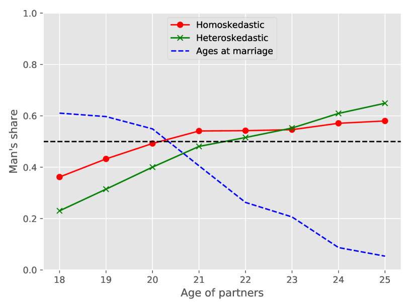
Figure 1: Men’s Share of the Marriage Surplus in the Logit Models

(a) The dashed blue line indicate the number of same-age marriages. The dashed black line corresponds to equal sharing of the surplus.

Figure 1 plots this ratio in the homoskedastic and in the heteroskedastic models for same-age couples ($x=y$). The surplus share of men clearly increases much more with age at marriage in the heteroskedastic version. Since the heteroskedastic model fits the data better, this suggests caution in interpreting the results of Choo and Siow (2006) on the effect of Roe vs Wade on the average utilities of men and women in marriage.

6.2 Flexible Multinomial Logit Models

Nested logit models assign equal correlation between all the alternatives in a given nest. This is not well-suited to the kind of correlations we would like to capture. What we need is a specification in which the preference shock for a partner of say age 22 is more positively correlated with the preference shock for a partner of age 23 than it is with the preference shock for a partner of age 29. In order to capture “age-local” correlations, we turned to the Flexible Coefficient Multinomial Logit (FC-MNL) model of Davis and Schiraldi (2014). This specification belongs to the class of Generalized Extreme Values models that we discussed in Appendix B.1. It allows for much more general substitution patterns between the different choices of partners, and in particular for “age-local” substitution patterns that we expect to find on the marriage market.

We estimated a few models of this family, along the lines suggested by Davis and Schiraldi (2014). All specifications we tried gave similar results; we present here the results we obtained where the matrix $\bm{b}$ that drives substitution patterns is given by

$$b^{x}_{y,y^{\prime}}=\begin{cases}\frac{b_{m}(x)}{\lvert y-y^{\prime}\rvert}&\mbox{ if }y\neq y^{\prime}\\ 1&\mbox{ if }y=y^{\prime};\end{cases}$$

where $b_{m}(x)$ is an affine function of the man’s age. We used a similar specification on women’s side, with an affine function $b_{w}(y)$ divided by $\lvert x-x^{\prime}\rvert$.

The maximum likelihood estimator of this model achieves a meager gain of $0.5$ point of the total loglikelihood over the basic Choo and Siow model. The affine functions are zero for the older men and women. Their estimated values for young men and women are positive but small. Still, they do suggest more subtle patterns of substitution between partners than the Choo and Siow model allows for. We illustrate this on Figures 2 and 3. Figure 2 for instance plots the “demand semi-elasticities”: $\partial\log\mu_{t|x}/\partial V_{y}$ for men whose age $x$ goes from 16 (in 1970) to 21. The horizontal and vertical axes represents partner’s ages $y$ and $t$ (five on each side of $x$, with the obvious truncation.)

In the Choo and Siow model, the semi-elasticities are given by the usual formula:

$$\frac{\partial\log\mu_{t|x}}{\partial V_{y}}=\mathrm{1\kern-3.99994pt1}(y=t)-\mu_{y|x}.$$

Aside from the diagonal $y=t$, the semi-elasticities do not depend on $t$. This appears as the vertical bands in the upper panel of Figure 2. The lower panel shows the same semi-elasticities for the FC-MNL model. Even with the small values of the $b$ coefficients we estimate, richer substitution patterns appear. Figure 3 tells a similar story for women.

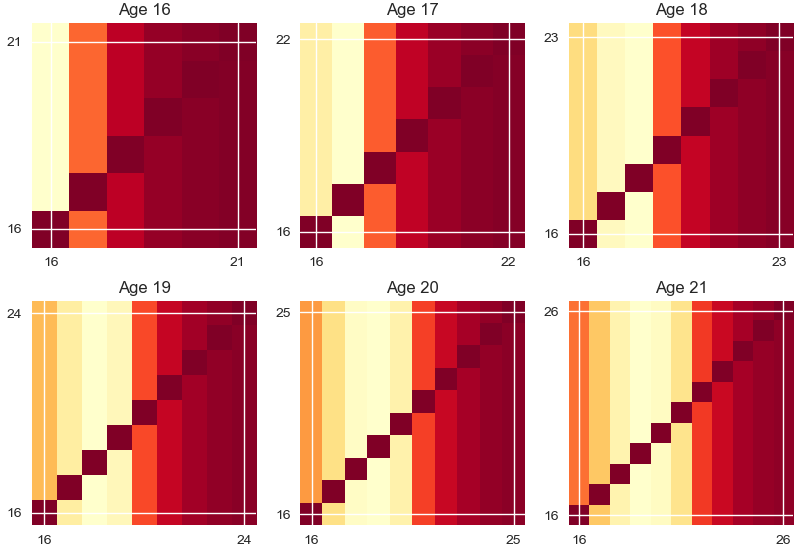
(a) Choo-Siow

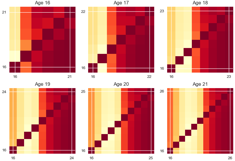
(b) FC-MNL

Figure 2: Semi-elasticities of substitution across partners: men

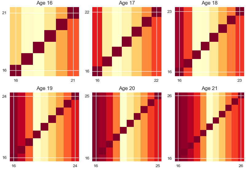
(a) Choo-Siow

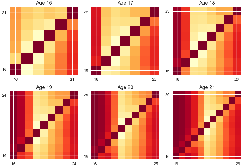
(b) FC-MNL

Figure 3: Semi-elasticities of substitution across partners: women

Concluding Remarks

Several assumptions made in our paper, in particular the separability assumption and the large market assumption are tested on simulations by Chiappori, Nguyen, and Salanié (2019). We find these simulation results reassuring about the assumptions we have maintained in the present paper. Other assumptions we made in the present paper can also be dispensed with. In particular, one challenge is to extend our analysis to the case where the observable characteristics of the partners may be continuous. This issue is addressed by Dupuy and Galichon (2014) for the Choo and Siow model, using the theory of extreme value processes; they also propose a test of the number of relevant dimensions for the matching problem. Our results also open the way to applications beyond the bipartite, one-to-one matching framework of this paper. Chiappori, Galichon, and Salanié (2019) for instance describe a formal analogy between the “roommate” (non-bipartite) problem and the bipartite one-to-one model. We expect that this framework should also prove useful in the study of trading on networks, when transfers are allowed (thus providing an empirical counterpart to Hatfield and Kominers (2012) and Hatfield, Kominers, Nichifor, Ostrovsky, and Westkamp (2013)). Finally, our assumption that utility is fully transferable without frictions can be relaxed. Galichon, Kominers, and Weber (2019) study models with imperfectly transferable utility and separable logit heterogeneity, while Galichon and Hsieh (2019) look at models with nontransferable utility and a similar form of heterogeneity.

Appendix

Appendix A Proofs

A.1 Proof of Proposition 1

Denote by $\left(\tilde{u}_{i}\right)$ and $\left(\tilde{v}_{j}\right)$ the equilibrium utilities of men and women. Stability requires that for all $(i,j)$,

• $\tilde{u}_{i}\geq\tilde{\Phi}_{i0}$, with equality if $i$ is single

• $\tilde{v}_{j}\geq\tilde{\Phi}_{0j}$, with equality if $j$ is single

• $\tilde{u}_{i}+\tilde{v}_{j}\geq\tilde{\Phi}_{ij}$, with equality if $i$ and $j$ are matched.

Let us focus on man $i$ in group $x$. This man must be single or matched. If he is matched, then $\tilde{u}_{i}=\max_{j}\left(\tilde{\Phi}_{ij}-\tilde{v}_{j}\right)$; and by Assumption 1, we have $\tilde{\Phi}_{ij}=\Phi_{xy_{j}}+\varepsilon_{iy_{j}}+\eta_{xj}$ so that

$$\tilde{u}_{i}=\max_{y}\left(\Phi_{xy}+\varepsilon_{iy}+\max_{j:y_{j}=y}\left(\eta_{xj}-\tilde{v}_{j}\right)\right).$$

If he is single, then $\tilde{u}_{i}=\tilde{\Phi}_{i0}=\varepsilon_{i0}$.

Let $V_{xy}=\inf_{j:y_{j}=y}\left(\tilde{v}_{j}-\eta_{xj}\right)$ and $V_{x0}=0$. Then

$$\tilde{u}_{i}=\max\left(\max_{y\in\mathcal{Y}}\left(\Phi_{xy}-V_{xy}+\varepsilon_{iy}\right),\varepsilon_{i0}\right)=\max_{y\in\mathcal{Y}_{0}}\left(\Phi_{xy}-V_{xy}+\varepsilon_{iy}\right).$$

Considering women would lead us to define $U_{xy}=\inf_{i:x_{i}=x}(\tilde{u}_{i}-\varepsilon_{iy})$ and $U_{0y}=0$. Since $\tilde{\Phi}_{ij}=\Phi_{x_{i}y_{j}}+\varepsilon_{iy_{j}}+\eta_{x_{i}j}$ cannot be larger than $\tilde{u}_{i}+\tilde{v_{j}}$, we obtain

$$\Phi_{x_{i}y_{j}}\leq(\tilde{u}_{i}-\varepsilon_{iy_{j}})+(\tilde{v}_{j}-\eta_{xj});$$ (A.1)

taking lower bounds gives $\Phi_{xy}\leq U_{xy}+V_{xy}$. Finally, if $\mu_{xy}>0$ then there is a couple $(i,j)$ with $x_{i}=x,y_{j}=y$ for which (A.1) is an equality, so that $\Phi_{xy}=U_{xy}+V_{xy}$.    

A.2 Proof of Theorem 1

Replacing the expression of $G$ given by (2.1) in formula (2.3) for $G^{\ast}$ gives

$$-G^{\ast}(\bm{\mu})=\inf_{\bm{\tilde{U}}}\left(-\sum_{y\in\mathcal{Y}_{0}}\mu_{y}\tilde{U}_{y}+\mathbb{E}_{\bm{P}}\max_{y\in\mathcal{Y}_{0}}\left(\varepsilon_{y}+\tilde{U}_{y}\right)\right)$$

where the minimization is over $\bm{\tilde{U}}$ such that $\tilde{U}_{0}=0$. The first term in the minimand can be seen as the expectation of the random variable $-\tilde{U}_{Y}$ under the distribution $Y\sim\mu_{Y}$. The term $\max_{y\in\mathcal{Y}_{0}}\left(\varepsilon_{y}+\tilde{U}_{y}\right)$ is the maximized utility of a man with mean utilities $\bm{\tilde{U}}$ and random taste shocks $\bm{\varepsilon}$. Alternatively, it is the value of the problem

$$\min\tilde{u}\;\mbox{ s.t.}\;\;\tilde{u}\geq\tilde{U}_{y}+\varepsilon_{y}\mbox{ for all }y\in\mathcal{Y}_{0},\mbox{ with one equality}.$$

Therefore

$$-G^{\ast}(\bm{\mu})=\inf_{\bm{\tilde{U},\tilde{u}}}\left(-\sum_{y\in\mathcal{Y}_{0}}\mu_{y}\tilde{U}_{y}+\mathbb{E}_{\bm{P}}\tilde{u}(\bm{\varepsilon})\right)$$

$$\;\mbox{ s.t.}\;\;\tilde{u}(\bm{\varepsilon})\geq\tilde{U}_{y}+\varepsilon_{y}\mbox{ for all }y\in\mathcal{Y}_{0},\bm{\varepsilon}.$$

Setting $V_{y}=-U_{y}$, we finally have

$$-G^{\ast}(\bm{\mu}) = \inf_{\bm{V},\tilde{u}}\left(\mathbb{E}_{\mu_{Y}}V_{Y}+\mathbb{E}_{\bm{P}}\tilde{u}(\bm{\varepsilon})\right)$$

$$\mbox{s.t.}~{}V_{0} = 0\;\mbox{ and }\;V_{y}+\tilde{u}(\bm{\varepsilon})\geq\varepsilon_{y}\;\;\;\forall y\in\mathcal{Y}_{0},\bm{\varepsilon}\in\mbox{supp}(\bm{P}).$$

This is exactly the value of the dual of an optimal transport problem in which the margins are $\mu_{Y}$ and $\bm{P}$ and the surplus $\varepsilon_{y}$ is split into $V_{y}$ and $\tilde{u}(\bm{\varepsilon})$. By the equivalence of the primal and the dual, this yields expression (2.6).    

A.3 Proof of Theorem 2

Since $\bm{P}$ has full support and is absolutely continuous, each $y$ achieves the maximum with positive probability; the function $G$ is strictly convex and by the envelope theorem, it is continuous differentiable and $\frac{\partial G}{\partial U_{y}}(\bm{U})$ is the probability that $y$ achieves the maximum. This is just the classical Daly-Zachary-Williams theorem. By the same token, $G^{\ast}$ is also strictly convex and continuously differentiable. The general theory of convex duality—or a straightforward application of the envelope theorem—tells us that $\mu_{y}=\left(\partial G/\partial\mu_{y}\right)(\bm{U})$ if and only if $U_{y}=\left(\partial G^{\ast}/\partial\mu_{y}\right)(\bm{\mu})$, which proves Part 2.

Now consider the strictly convex function $\bm{\tilde{U}}\longmapsto G\left(\bm{\tilde{U}}\right)-\sum_{y\in\mathcal{Y}}\mu_{y}\tilde{U}_{y}$. Part 3 follows from the fact that by the envelope theorem, $\bm{U}$ minimizes the value of this function if and only if $U_{y}=\left(\partial G^{\ast}/\partial\mu_{y}\right)(\bm{\mu})$. Since $G(\bm{U})=\mathbb{E}_{\bm{P}}\max_{y\in\mathcal{Y}_{0}}(U_{y}+\varepsilon_{y})$, defining $\tilde{u}(\bm{\varepsilon})$ as in our proof of Theorem 1 yields (2.9).    

A.4 Proof of Theorem 3

In this proof we denote $\tilde{n}$ the distribution of $\left(x,\bm{\varepsilon}\right)$ when the distribution of $x$ is $\bm{n}$ and the distribution of $\bm{\varepsilon}$ conditional on $x$ is $\bm{P}_{x}$. Formally, for $S\subseteq\mathcal{X}\times\mathbb{R}^{\mathcal{Y}_{0}}$, we get

$$\tilde{n}\left(S\right)=\sum_{x}n_{x}\int_{\mathbb{R}^{\mathcal{Y}_{0}}}\mathrm{1\kern-3.99994pt1}\left(x,\bm{\varepsilon}\in S\right)d\bm{P}_{x}\left(\bm{\varepsilon}\right).$$

We define $\tilde{m}$ in the same way.

By the dual formulation of the matching problem (see Gretsky, Ostroy, and Zame (1992)), the value of total welfare in equilibrium is obtained by solving

$$\mathcal{W}=\inf_{\tilde{u},\tilde{v}} \left(\int\tilde{u}\left(x,\bm{\varepsilon}\right)d\tilde{n}\left(x,\bm{\varepsilon}\right)+\int\tilde{v}\left(y,\bm{\eta}\right)d\tilde{m}\left(y,\bm{\eta}\right)\right)$$ (A.2)

s.t. $$\tilde{u}\left(x,\bm{\varepsilon}\right)+\tilde{v}\left(y,\bm{\eta}\right)\geq\Phi_{xy}+\varepsilon_{y}+\eta_{x}\;\;\forall(x,y,\bm{\varepsilon},\bm{\eta})$$

$$\tilde{u}\left(x,\bm{\varepsilon}\right)\geq\varepsilon_{0}\;\;\forall(x,\bm{\varepsilon})$$

$$\tilde{v}\left(y,\bm{\eta}\right)\geq\eta_{0}\;\;\forall(y,\bm{\eta}).$$

Fix any $\tilde{u},\tilde{v}$ that satisfies all constraints in this program. As in the proof of Proposition 1, for $x\in\mathcal{X}$ and $y\in\mathcal{Y}$ we define

$$U_{xy}=\inf_{\bm{\varepsilon}}\left\{\tilde{u}\left(x,\bm{\varepsilon}\right)-\varepsilon_{y}\right\}\mbox{ and }V_{xy}=\inf_{\bm{\eta}}\left\{\tilde{v}\left(y,\bm{\eta}\right)-\eta_{x}\right\};$$

and we let $U_{x0}=V_{0y}=0$. Then $\tilde{u}\left(x,\bm{\varepsilon}\right)\geq\max_{y\in\mathcal{Y}_{0}}\left\{U_{xy}+\varepsilon_{y}\right\}$ and $\tilde{v}\left(y,\bm{\eta}\right)\geq\max_{x\in\mathcal{X}_{0}}\left\{V_{xy}+\eta_{x}\right\}$; and the first constraint in (A.2) is simply $U_{xy}+V_{xy}\geq\Phi_{xy}$. Reciprocally, assume that $U_{x0}=V_{0y}=0$ and $U_{xy}+V_{xy}\geq\Phi_{xy}$ for all $x\in\mathcal{X}$ and $y\in\mathcal{Y}$, and define

$$\tilde{u}\left(x,\bm{\varepsilon}\right)=\max_{y\in\mathcal{Y}_{0}}\left\{U_{xy}+\varepsilon_{y}\right\}\;\mbox{ and }\;\tilde{v}\left(y,\bm{\eta}\right)\geq\max_{x\in\mathcal{X}_{0}}\left\{V_{xy}+\eta_{x}\right\};$$

Then $(\tilde{u},\tilde{v})$ satisfies all constraints. Therefore we can rewrite the whole program as:

$$\mathcal{W} = \min_{U,V}\left(\int\max_{y\in\mathcal{Y}_{0}}\left\{U_{xy}+\varepsilon_{y}\right\}d\tilde{n}\left(x,\bm{\varepsilon}\right)+\int\max_{x\in\mathcal{X}_{0}}\left\{V_{xy}+\eta_{x}\right\}d\tilde{m}\left(y,\bm{\eta}\right)\right)$$

s.t. $$U_{xy}+V_{xy}\geq\Phi_{xy}~{}\forall x\in\mathcal{X},y\in\mathcal{Y}$$

and $$U_{x0}=V_{0y}=0~{}\forall x\in\mathcal{X},y\in\mathcal{Y}.$$

Now remember that we defined $G_{x}(\bm{U}_{x\cdot})=\int\max_{y\in\mathcal{Y}_{0}}(U_{xy}+\varepsilon_{y})dP_{x}(\bm{\varepsilon})$ and $G(\bm{U},\bm{n})=\sum_{x}n_{x}G_{x}(\bm{U}_{x\cdot}).$ Under Assumption 1,

$$\left|\max_{y\in\mathcal{Y}_{0}}\left(U_{xy}+\varepsilon_{y}\right)\right|\leq\max_{y\in\mathcal{Y}_{0}}\lvert U_{xy}\rvert+\max_{y\in\mathcal{Y}_{0}}\lvert\varepsilon_{y}\rvert$$

is integrable, so that $G_{x}$ is well-defined. It follows that

$$\mathcal{W} = \min_{U,V}\left(G\left(\bm{U},\bm{n}\right)+H\left(\bm{V},\bm{m}\right)\right)$$

s.t. $$U_{xy}+V_{xy}\geq\Phi_{xy}~{}\forall x\in\mathcal{X},y\in\mathcal{Y}$$

which is expression (3.6). Introducing multipliers $(\mu_{xy})$, this convex minimization problem can be written in a minimax form as

$$\mathcal{W} = \min_{\bm{U},\bm{V}}\max_{\mu\geq 0}\left(G\left(\bm{U},\bm{n}\right)+H\left(\bm{V},\bm{m}\right)+\sum_{xy}\mu_{xy}\Phi_{xy}-\sum_{xy}\mu_{xy}U_{xy}-\sum_{xy}\mu_{xy}V_{xy}\right)$$

$$= \max_{\bm{\mu}\geq 0}\left(\sum_{xy}\mu_{xy}\Phi_{xy}-\max_{\bm{U},\bm{V}}\left(\sum_{xy}\mu_{xy}U_{xy}+\sum_{xy}\mu_{xy}V_{xy}-G\left(\bm{U},\bm{n}\right)-H\left(\bm{V},\bm{m}\right)\right)\right)$$

which is (3.5); and (3.7) are its first-order conditions.    

A.5 Proof of Proposition 2

Part (i) and $U_{xy}+V_{xy}=\Phi_{xy}$ restate Proposition 1 (since Assumption 2 guarantees that $\mu_{xy}>0$ for all $(x,y)\in\mathcal{A}$). For part (ii), note that applying the envelope theorem twice,

$$\frac{\partial\mathcal{W}}{\partial n_{x}}=-\frac{\partial G^{\ast}}{\partial n_{x}}=\frac{\partial G}{\partial n_{x}}$$

which equals $G_{x}$ by the definition (3.1). Part (iii) is similar.    

A.6 Proof of Theorem 4

Part (i) follows from Theorem 2 (ii). Moreover, the $\bm{\mu}$’s are the multipliers in (3.6); since they are all positive, the constraints must be saturated, proving (ii).    

A.7 Extending the Entropy

Lemma 1 below is instrumental in the derivation of an efficient algorithm in Section 4.2.

While the generalized entropy $\mathcal{E}$ defined in (3.4) is concave in the matching patterns $\bm{\mu}$, it is only strictly concave when $\bm{\mu}$ has the margins $\bm{r}$ (otherwise $\mathcal{E}$ is infinite). We will need to extend it to a function that is strictly concave everywhere.

Definition 2 (Extended Entropy).

Let $\mathcal{\ E}(\bm{\mu};\bm{r})$ be the generalized entropy of matching. We say that a function $E$ extends $\mathcal{E}$ if it is a strictly concave function of $\bm{\mu}$ that coincides with over the set of feasible matchings $\bm{\mu}\in\mathcal{M}(\bm{r})$.

There are many ways of extending a given generalized entropy function $\mathcal{E}$. Any choice of

$$E\left(\bm{\mu};\bm{r}\right)=\mathcal{E}\left(\bm{\mu},\sum_{y}\mu_{xy}+\mu_{x0},\sum_{x}\mu_{xy}+\mu_{0y}\right)+K\left(\bm{\mu};\bm{r}\right)$$

will work, where

$$K\left(\bm{\mu};\bm{r}\right)=\sum_{x}\left\{A_{x}\left(\sum_{y}\mu_{xy}+\mu_{x0}\right)-A_{x}\left(n_{x}\right)\right\}+\sum_{y}\left\{B_{y}\left(\sum_{x}\mu_{xy}+\mu_{0y}\right)-B_{y}\left(m_{y}\right)\right\},$$ (A.3)

and $A_{x}$ and $B_{y}$ are concave functions from $\mathbb{R}$ to $\mathbb{R}$. Defining $E$ in this way ensures that it coincides with $\mathcal{E}(\bm{\mu},\bm{r})$ for any feasible matching; and adding the term $K$ makes $E$ strictly concave in $\bm{\mu}$.

Lemma 1.

Let $E$ extend $\mathcal{E}$. For $\bm{u}\in\mathrm{I\kern-1.69998ptR}^{\mathcal{X}}$ and $\bm{v}\in\mathrm{I\kern-1.69998ptR}^{\mathcal{Y}}$, define $S(\bm{u},\bm{v})$ as the value of

$$\max_{\bm{\mu}}\left(E(\bm{\mu};\bm{r})+\sum_{x,y\in\mathcal{X}\times\mathcal{Y}}\mu_{xy}(\Phi_{xy}-u_{x}-v_{y})+\sum_{x\in\mathcal{X}}(n_{x}-\mu_{x0})u_{x}+\sum_{y\in\mathcal{Y}}(m_{y}-\mu_{0y})v_{y}\right).$$ (A.4)

Then $S$ is a convex function of $(\bm{u},\bm{v})$. The social welfare $\mathcal{W}$ is its minimum value; the minimizers $\bm{u}$ and $\bm{v}$ are the average utilities of the different types of men and women in equilibrium; and the solutions $\bm{\mu}$ to (A.4) at $(\bm{u},\bm{v})$ are the equilibrium matching patterns.

• Recall from equation (3.5) that the equilibrium matching $\bm{\mu}$ maximizes $\sum_{x,y}\mu_{xy}\Phi_{xy}+\mathcal{E}(\bm{\mu},\bm{r})$ over $\mu$ in $\mathbb{R}^{\mathcal{X}\times\mathcal{Y}}$. This can be rewritten as

  $$\max_{\bm{\mu}} \sum_{x,y\in\mathcal{X}\times\mathcal{Y}}\mu_{xy}\Phi_{xy}+E(\bm{\mu};\bm{r})$$ (A.5)

  $$s.t.~{} \mu_{x0}+\sum_{y\in\mathcal{Y}}\mu_{xy}=n_{x}$$

  $$\mu_{0y}+\sum_{x\in\mathcal{X}}\mu_{xy}=m_{y}.$$

  Denote $a_{x}$ and $b_{y}$ the multipliers of the constraints. The Lagrangian of (A.5) can be written as

  $$\mathcal{L} =\max_{\bm{\mu}}\min_{\bm{a},\bm{b}}\left(\begin{array}[]{c}\sum_{x,y\in\mathcal{X}\times\mathcal{Y}}\mu_{xy}\Phi_{xy}+E(\bm{\mu};\bm{r})\\ -\sum_{x\in\mathcal{X}}a_{x}\left(\mu_{x0}+\sum_{y\in\mathcal{Y}}\mu_{xy}-n_{x}\right)-\sum_{y\in\mathcal{Y}}b_{y}\left(\mu_{0y}+\sum_{x\in\mathcal{X}}\mu_{xy}-m_{y}\right)\end{array}\right)$$

  $$=\max_{\bm{\mu}}\min_{\bm{a},\bm{b}}\left(\begin{array}[]{c}\sum_{x,y\in\mathcal{X}\times\mathcal{Y}}\mu_{xy}\left(\Phi_{xy}-a_{x}-b_{y}\right)+E(\bm{\mu};\bm{r})\\ +\sum_{x\in\mathcal{X}}a_{x}\left(n_{x}-\mu_{x0}\right)+\sum_{y\in\mathcal{Y}}b_{y}\left(m_{y}-\mu_{0y}\right)\end{array}\right).$$

  Interchanging $\min$ and $\max$ gives $\mathcal{L}=\min_{\bm{a},\bm{b}}S(\bm{a},\bm{b};\bm{\Phi},\bm{r})$, where $S$ is defined in the corollary. It is a maximum of linear functions of $\bm{a},\bm{b}$ and therefore convex. Since the constraints are binding at the optimum, $\mathcal{W}=\mathcal{L}$. Moreover, by the envelope theorem $\frac{\partial\mathcal{W}}{\partial n_{x}}=\frac{\partial S}{\partial n_{x}}=a_{x}$. By Proposition 2, this gives $a_{x}=u_{x}$; and the $\mu$’s are the corresponding matching patterns.

A.8 Proof of Theorem 5

We start by extending the generalized entropy $\mathcal{E}$ to a strictly concave function $E$ as explained in A.7. For notational simplicity, we now drop the arguments $\bm{r}$ and $\bm{\Phi}$. Proposition 1 shows that the value of the matching problem is $\min_{\bm{a},\bm{b}}S(\bm{a},\bm{b})$. We solve for the minimum iteratively by coordinate descent. At step $2k$, we first fix $\bm{b}=\bm{b}^{(2k)}$ and we solve the convex minimization problem over $\bm{a}$ only:

$$\bm{a}^{(2k+1)}\equiv\arg\min_{\bm{a}}S(\bm{a},\bm{b}^{(2k)}).$$

Then we keep $\bm{a}=\bm{a}^{(2k+1)}$ fixed at this new value and we solve the minimization problem over $\bm{b}$:

$$\bm{b}^{(2k+2)}\equiv\arg\min_{\bm{b}}S(\bm{a}^{(2k+1)},\bm{b}).$$

We stop the iterations when $\bm{b}^{(2k+2)}$ and $\bm{b}^{(2k)}$ are close enough. We take $\bm{u}^{(2k+1)}$ and $\bm{v}^{(2k+2)}$ to be the average utilities, and the associated $\bm{\mu}$ to be the equilibrium matching patterns.

Let us now prove that the algorithm converges to the global minimum $(\bm{u},\bm{v})$ of $S$. We rely on results in Bauschke and Borwein (1997), which builds on Csiszár (1975). The map $\bm{\mu}\rightarrow-E(\bm{\mu})$ is smooth and strictly convex; hence it is a “Legendre function” in their terminology. Introduce the associated “Bregman divergence” $D$ as

$$D\left(\bm{\mu},\bm{\bar{\nu}}\right)=E\left(\bm{\bar{\nu}}\right)-E\left(\bm{\mu}\right)+\left\langle\nabla E\left(\bm{\bar{\nu}}\right),\bm{\mu}-\bm{\bar{\nu}}\right\rangle,$$

where $\nabla$ denotes the gradient wrt $\bm{\bar{\nu}}$; and define the linear subspaces $\mathcal{L}\left(\bm{n}\right)$ and $\mathcal{L}\left(\bm{m}\right)$ by

$$\mathcal{L}\left(\bm{n}\right)=\{\bm{\mu}\geq 0:\forall x\in\mathcal{X},~{}\sum_{y\in\mathcal{Y}_{0}}\mu_{xy}=n_{x}\}\text{ and }\mathcal{L}\left(\bm{m}\right)=\{\bm{\mu}\geq 0:\forall y\in\mathcal{Y},~{}\sum_{x\in\mathcal{X}_{0}}\mu_{xy}=m_{y}\}$$

so that $\mathcal{M}(\bm{r})=\mathcal{L}\left(\bm{n}\right)\cap\mathcal{L}\left(\bm{m}\right)$. It is easy to see that $\bm{\mu}^{(k)}$ results from iterative projections with respect to $D$ on the linear subspaces $\mathcal{L}(\bm{n})$ and $\mathcal{L}(\bm{m})$:

$$\bm{\mu}^{(2k+1)}=\arg\min_{\bm{\mu}\in\mathcal{L}\left(\bm{n}\right)}D\left(\bm{\mu},\bm{\mu}^{(2k)}\right)\text{ and }\bm{\mu}^{(2k+2)}=\arg\min_{\bm{\mu}\in\mathcal{L}\left(\bm{m}\right)}D\left(\bm{\mu},\bm{\mu}^{(2k+1)}\right).$$ (A.6)

By Theorem 8.4 of Bauschke and Borwein, the iterated projection algorithm converges to the projection $\bm{\mu}$ of $\bm{\mu}^{(0)}$ on $\mathcal{M}(\bm{r})$, which is also the maximizer $\bm{\mu}$ of (3.5).

As mentioned earlier, there are many possible ways of extending $\mathcal{E}$ to $E$, depending on the choice of the functions $A_{x}$ and $B_{y}$ in (A.3). In practice, good judgement should be exercised, as the choice of an extension $E$ that makes it easy to solve the systems in A.6 is crucial for the performance of the algorithm.

Appendix B Examples of random utility models

B.1 The Generalized Extreme Value Framework

Consider a function $g:\mathbb{R}^{\mathcal{Y}_{0}}\rightarrow\mathbb{R}$ that (i) is positive homogeneous of degree one; (ii) goes to $+\infty$ whenever any of its arguments goes to $+\infty$; (iii) has partial derivatives (outside of $\bm{0}$) at any order $k$ of sign $\left(-1\right)^{k}$; (iv) is such that the function defined by $F\left(w_{0},\ldots,w_{\lvert\mathcal{Y}\rvert}\right)=\exp\left(-g\left(e^{-w_{0}},\ldots,e^{-w_{\lvert\mathcal{Y}\rvert}}\right)\right)$ is a multivariate cumulative distribution function associated to some distribution, which we denote $\bm{P}$. Then introducing utility shocks $\bm{\varepsilon}\sim\bm{P}$, we have by a theorem of McFadden (1978):

$$G(\bm{w})=\mathbb{E}_{\bm{P}}\left[\max_{y\in\mathcal{Y}_{0}}\left\{w_{y}+\varepsilon_{y}\right\}\right]=\log g\left(e^{\bm{w}}\right)+\gamma$$ (B.1)

where $\gamma$ is the Euler constant $\gamma\simeq 0.577$.

For any vector $\bm{p}\in\mathrm{I\kern-1.69998ptR}^{\mathcal{Y}}$ such that $\sum_{y\in\mathcal{Y}}p_{y}=1$, we denote $\bm{\bar{p}}=(p_{1},\ldots,p_{\lvert\mathcal{Y}\rvert})$. Then

$$G^{\ast}\left(\bm{\bar{p}}\right)=\log g\left(e^{\bm{w}\left(\bm{p}\right)}\right)+\gamma-\sum_{y\in\mathcal{Y}_{0}}p_{y}w_{y}\left(\bm{p}\right),$$

where the vector $\bm{w}\left(p\right)$ solves the system of equations

$$p_{y}=\frac{\partial\log g}{\partial w_{y}}\left(e^{\bm{w}}\right)\;\mbox{ for all }\;y\in\mathcal{Y}_{0}.$$ (B.2)

Now take a vector $\bm{\mu}=(\mu_{y})_{y\in\mathcal{Y}}$ such that $\sum_{y\in\mathcal{Y}}\mu_{y}\leq 1$. The generalized entropy of choice arising from this heterogeneity is

$$G^{\ast}(\bm{\mu})=\log g\left(e^{\bm{w}\left(\bm{\mu}\right)}\right)-\sum_{y\in\mathcal{Y}_{0}}\mu_{y}w_{y}\left(\bm{\mu}\right)+\gamma.$$ (B.3)

Applying the envelope theorem, the derivative of this expression with respect to $\mu_{y}$ is $-w_{y}\left(\bm{\mu}\right)$. Therefore the $\bm{U}$ vector is identified by

$$U_{y}=w_{y}\left(\bm{\mu}\right).$$ (B.4)

B.2 The nested logit model

We consider the two-layer nested logit model of Example 2.1: alternative $0$ is alone in a nest and each other nest $n\in\mathcal{N}$ contains alternatives $y\in\mathcal{Y}\left(n\right)$. The correlation of alternatives whithin nest $n$ is proxied by $(1-\lambda_{n}^{2})$.

B.2.1 The entropy of choice of the one-sided nested logit model

It is well-known that

$$G(\bm{U})=\log\left(1+\sum_{n\in\mathcal{N}}\exp(I_{n}(\bm{U}))\right)$$

where $I_{n}(\bm{U})\equiv\lambda_{n}\log\left(\sum_{y\in\mathcal{Y}\left(n\right)}\exp(U_{y}/\lambda_{n})\right)$ is the inclusive value of nest $n$. For $y\in\mathcal{Y}_{n}$, this gives

$$\mu_{y}=\frac{\partial G}{\partial U_{y}}(\bm{U})=\mu_{n}\times\frac{\exp(U_{y}/\lambda_{n})}{\exp\left(I_{n}(\bm{U})/\lambda_{n}\right)},$$

where

$$\mu_{n}:=\sum_{y\in\mathcal{Y}\left(n\right)}\mu_{y}=\frac{\exp\left(I_{n}(\bm{U})\right)}{1+\sum_{m\in\mathcal{N}}\exp\left(I_{m}(\bm{U})\right)}.$$

As a result, $\log\mu_{n}=I_{n}(\bm{U})-G(\bm{U})$ and $\log\mu_{y}=\log\mu_{n}+(U_{y}-I_{n}(\bm{U}))/\lambda_{n}$. Moreover,

$$\mu_{0}=1-\sum_{n\in\mathcal{N}}\mu_{n}=\exp(-G(\bm{U})),$$

so that we can solve for

$$G(\bm{U}) =-\log\mu_{0}$$

$$I_{n}(\bm{U}) =\log(\mu_{n}/\mu_{0})$$

$$U_{y} =\lambda_{n}\log\frac{\mu_{y}}{\mu_{0}}+\left(1-\lambda_{n}\right)\log\frac{\mu_{n}}{\mu_{0}}.$$ (B.5)

Since $G^{\ast}(\bm{\mu})=\sum_{y\neq 0}\mu_{y}U_{y}-G(\bm{U})$ at the optimum, this gives

$$G^{\ast}(\bm{\mu}) =\sum_{n\in\mathcal{N}}\lambda_{n}\sum_{y\in\mathcal{Y}(n)}\mu_{y}\log\mu_{y}-\left(\sum_{y\neq 0}\mu_{y}\right)\log\mu_{0}$$

$$+\sum_{n\in\mathcal{N}}(1-\lambda_{n})\left(\sum_{y\in\mathcal{Y}(n)}\mu_{y}\right)\log\mu_{n}+\log\mu_{0};$$

using $\sum_{y\neq 0}\mu_{y}=1-\mu_{0}$ and $\sum_{y\in\mathcal{Y}(n)}\mu_{y}=\mu_{n}$, we get the generalized entropy of choice

$$G^{\ast}(\bm{\mu})=\sum_{n\in\mathcal{N}}\left(\lambda_{n}\sum_{y\in\mathcal{Y}(n)}\mu_{y}\log\mu_{y}+(1-\lambda_{n})\mu_{n}\log\mu_{n}\right)+\mu_{0}\log\mu_{0}.$$

B.2.2 The two-sided nested logit model

Now suppose that the above (indexed by $x$ as $\lambda_{n}^{x},\mathcal{N}^{x},\mathcal{Y}^{x}(n)$) describes the structure of errors for men of group $x$, and that women of group $y$ have a similar error structure with parameters $\nu_{n}^{y},\mathcal{N}^{y},\mathcal{X}^{y}(n)$. We denote $n(y;x)$ the nest of partner group $y$ for men of group $x$, and $n(x;y)$ the nest of partner group $x$ for women of group $y$. Then the matrix $\bm{U}$ is identified as

$$U_{xy}=\lambda^{x}_{n(y;x)}\log\frac{\mu_{xy}}{\mu_{x0}}+\left(1-\lambda^{x}_{n(y;x)}\right)\log\frac{\mu_{x,n(y;x)}}{\mu_{x0}}.$$

Along with the corresponding formula for $\bm{V}$, this identifies the joint surplus as

$$\Phi_{xy} =(\lambda^{x}_{n(y;x)}+\nu^{y}_{n(x;y)})\log\mu_{xy}-\log\mu_{x0}-\log\mu_{0y}$$

$$+\left(1-\lambda^{x}_{n(y;x)}\right)\log\mu_{x,n(y;x)}+\left(1-\nu^{y}_{n(x;y)}\right)\log\mu_{n(x;y),y}$$

for any given values of the parameters of the nested logit errors.

B.3 The random coefficients logit model

Recall that Example 2.2 had $\bm{\varepsilon}=\bm{Z}\bm{e}+T\bm{\eta}$, where $\bm{e}$ is a random vector on $\mathbb{R}^{d}$ with distribution $\mathbf{P}_{\epsilon}$; $\bm{Z}$ is a $\left|\mathcal{Y}_{0}\right|\times d$ matrix; $T>0$; and $\bm{\eta}$ is an extreme value type-I (Gumbel) random variable i.i.d. on $\mathbb{R}^{\mathcal{Y}_{0}}$ and independent from $\bm{e}$.

By the law of iterated expectations, making use of the independence of $\bm{e}$ and $\bm{\eta}$, we get

$$G\left(\bm{U}\right) = \mathbb{E}\left[\mathbb{E}\left[\max_{y\in\mathcal{Y}_{0}}\left\{U_{y}+\left(\bm{Z}\bm{e}\right)_{y}+T\eta_{y}\right\}|\bm{e}\right]\right]$$ (B.6)

$$= \int G_{0}\left(U+\bm{Z}\bm{e}\right)f\left(e\right)de$$ (B.7)

where

$$G_{0}\left(\bm{U}\right)=T\log\sum_{y\in\mathcal{Y}_{0}}\exp\left(\frac{U_{y}}{T}\right)$$

is the Emax operator associated with the plain multinomial logit model. It is easy to compute its convex conjugate: $G_{0}^{\ast}\left(\bm{\pi}\right)=T\sum_{y}\pi_{y}\log\pi_{y}$ if $\sum_{y}\pi_{y}=1$, and $+\infty$ otherwise.

We will use two well-known properties of convex conjugates (see e.g. Hiriart-Urruty and Lemaréchal, 2001, part E):

• the convex conjugate of a translated function $\bm{x}\to g_{t}(\bm{x})\equiv g(\bm{x}+\bm{t})$ is $g_{t}^{\ast}(\bm{y})=g^{\ast}(\bm{y})+\bm{y}\cdot\bm{t}$

• the convex conjugate of a sum of convex functions is the infimum-convolution of their convex conjugates:

  $$(f_{1}+f_{2})^{\ast}(\bm{y})=\inf_{\bm{y}_{1}+\bm{y}_{2}=\bm{y}}\left(f_{1}^{\ast}(\bm{y}_{1})+f_{2}^{\ast}(\bm{y}_{2})\right).$$

Together, they imply that

$$G^{\ast}\left(\bm{\mu}\right)=\inf_{\bm{\pi}(\cdot)\geq 0}\left\{\int G_{0}^{\ast}\left(\bm{\pi}(\bm{e})\right)d\bm{P}_{\bm{e}}(\bm{e})-\sum_{y}\int\left(Ze\right)_{y}\pi_{y}\left(\bm{e}\right)d\bm{P}_{\bm{e}}(\bm{e}):\;\int_{\bm{e}}\pi_{y}\left(\bm{e}\right)d\bm{P}_{\bm{e}}(\bm{e})=\mu_{y}\;\forall y\right\}.$$ (B.8)

It follows that

$$-G^{\ast}\left(\bm{\mu}\right) = \max_{\bm{\pi}(\cdot)\geq 0}\left\{\sum_{y}\int\left(Ze\right)_{y}\pi_{y}\left(\bm{e}\right)-T\sum_{y}\pi_{y}\left(\bm{e}\right)\log\pi_{y}\left(\bm{e}\right)\right\}d\bm{P}_{\bm{e}}(\bm{e})$$

$$s.t. \int\pi_{y}\left(\bm{e}\right)d\bm{P}_{\bm{e}}(\bm{e})=\mu_{y}\;\forall y$$

$$\sum_{y}\pi_{y}\left(\bm{e}\right)=1\;\forall\bm{e}.$$

This is an optimal transport problem with entropic regularization, (see Galichon, 2016, Chapter 7). In the absence of the second term in the objective function, it would be an optimal transport problem between the discrete random variable $Y\sim\bm{\mu}$ and the continuous random vector $\bm{e}\sim\bm{P}_{\bm{e}}$, with transport surplus $\left(y,\bm{e}\right)\rightarrow-\left(\bm{Z}\bm{e}\right)_{y}$. The second term is an entropic regularization.

B.4 The pure characteristics model

The second part of Example 2.2 is obtained by setting $T=0$ in (B.7). The regularization term in (B.8) disappears, and

$$G^{\ast}(\bm{\mu})=\max_{\bm{\pi}\in\mathcal{M}}\sum_{y\in\mathcal{Y}_{0}}\mu_{y}\int_{\bm{e}\in\mathbb{R}^{d}}-\left(Z\bm{e}\right)d\bm{P}_{\bm{e}}\left(\bm{e}\right)$$ (B.9)

which is a standard optimal transport problem (this time without the entropic regularization) between a discrete random variable on $\mathbb{R}^{d}$ $\tilde{z}$ such that $\tilde{z}_{i}=Z_{\tilde{y}i}$ where $\tilde{y}\sim\mu$, and the continuous random variable $\bm{e}\sim\bm{P}$, where the transport surplus is now the scalar product $\left(z,\bm{e}\right)\rightarrow z^{\top}\epsilon$. This is exactly the power diagram situation described in Chapter 5 of Galichon (2016).

B.5 The FC-MNL Model

Davis and Schiraldi (2014) introduced a flexible GEV specification which they called the Flexible Coefficients-Multinomial Choice Model.

Example B.1 (FC-MNL).

The function $g$ that appears in (B.1) takes the following form:

$$g(\bm{t})=\sum_{(y,y^{\prime})\in\mathcal{Y}_{0}^{2}}b_{y,y^{\prime}}\left(\frac{t_{y}^{1/\sigma}+t_{y^{\prime}}^{1/\sigma}}{2}\right)^{\tau\sigma}$$

where $(b_{y,y^{\prime}})$ is a non-negative symmetric matrix, and the parameters satisfy the inequalities $0<\sigma<1$, $\tau>1$, $\tau\sigma\leq 1$. We can set $b_{yy}=1$ for every $y$. Note that we recover the standard multinomial logit model when $\bm{b}$ is the identity matrix.

We followed Davis and Schiraldi (2014) in making $g$ a $\tau$-homogeneous function, rather than 1-homogeneous. This is a harmless normalization. It gives

$$G(\bm{U})=\frac{1}{\tau}\left(\log\sum_{(y,y^{\prime})\in\mathcal{Y}_{0}^{2}}b_{y,y^{\prime}}\left(\frac{\exp(U_{y}/\sigma)+\exp(U_{y^{\prime}}/\sigma)}{2}\right)^{\tau\sigma}\right)+\gamma.$$

While this may look forbidding, it is easy to evaluate and it yields simple demands:

$$\mu_{y}=\frac{1}{g}\exp(U_{y}/\sigma)\sum_{y^{\prime}\in\mathcal{Y}_{0}}b_{y,y^{\prime}}\left(\frac{\exp(U_{y}/\sigma)+\exp(U_{y^{\prime}}/\sigma)}{2}\right)^{\tau\sigma-1}.$$

It is apparent from the formulæ that the “cross-price elasticities” (the dependence of $\bm{\mu}$ on $\bm{U}$ are largely driven by the matrix $\bm{b}$.) In fact Davis and Schiraldi (2014) show that for any fixed $\sigma$ and $\tau$, $\bm{b}$ can be chosen to replicate any given set of own- and cross-price elasticities.

Suggested online appendices

Appendix C More on the assumptions [online]

In this online appendix, we discuss the separability assumption (which we maintain throughout), and the type I extreme value assumption of Choo and Siow (2006) (which we relax).

C.1 The separability assumption

Assumption 1 imposes that the matching surplus $\tilde{\Phi}$ be separable in the sense that

$$\tilde{\Phi}_{ij}=\Phi_{xy}+\varepsilon_{iy}+\eta_{xj}.$$

It is easy to see that Assumption 1 is equivalent to the follwing:

Assumption 3 (Separability restated).

If two men $i$ and $i^{\prime}$ belong to the same group $x$, and their respective partners $j$ and $j^{\prime}$ belong to the same group $y$, then the total surplus generated by these two matches is unchanged if partners are shuffled:

$$\tilde{\Phi}_{ij}+\tilde{\Phi}_{i^{\prime}j^{\prime}}=\tilde{\Phi}_{ij^{\prime}}+\tilde{\Phi}_{i^{\prime}j}.$$

It should be clear from this equivalent definition that we need not adopt Choo and Siow’s original interpretation, in which $\bm{\varepsilon}$ was a vector of preference shocks of the husband and $\bm{\eta}$ was a vector of preference shocks of the wife. More precisely, they assumed that the utility of a man $i$ of group $x$ who marries a woman $j$ of group $y$ was given by

$$\alpha_{xy}+\tau+\varepsilon_{iy},$$ (C.1)

where $\alpha_{xy}$ was the “systematic” part of the surplus; $\tau$ represented the utility transfer (possibly negative) that the husband gets from his partner in equilibrium; and $\varepsilon_{iy}$ was a standard type I extreme value random term. The utility of this man’s wife would be written as

$$\gamma_{xy}-\tau+\eta_{xj}.$$ (C.2)

This formulation clearly implies separability, but it is much stronger than we need. To take an extreme example, assume that men are indifferent over partners and are only interested in the transfer they receive; while women also care about some attractiveness characteristic of men, in a way that may depend on the woman’s group. In a marriage between man $i$ of group $x$ and woman $j$ of group $y$, if the wife transfers $\tau$ to the husband his net utility would be $\tau$, and hers would be $(\varepsilon_{iy}-\tau$). Since the joint surplus is $\varepsilon_{iy}$, it clearly satisfies Assumption 1. All of our results would apply in this case. Since there is a continuum of women in each group $y$, but only one man $i$, he must capture all joint surplus if he marries a woman of group $y$: his net utility must be $\varepsilon_{iy}$, and hers zero. In other words, this man will receive a transfer $\tau_{i}=\max_{y\in\mathcal{Y}}\varepsilon_{iy}$, which depends on his unobservable characteristic. In contrast, in Choo and Siow’s preferred interpretation equilibrium transfers only depend on characteristics that are observed by the analyst. Once again, this is a matter of modelling choice and not a logical necessity since the $\bm{\varepsilon}$ and $\bm{\eta}$ terms are observed by all agents.

C.2 The logit assumption

A second major assumption in the Choo and Siow model states that the distribution of the unobserved heterogeneity terms $\varepsilon_{iy}$ and $\eta_{xj}$ are distributed as type I extreme value iid random vectors. This brings in familiar but restrictive features of the logit model, and in particular, the Independence of Irrelevant Alternatives (IIA) property.

The literature on single-agent discrete choice models has long stressed the links between the type I-EV specification and IIA. In his famous discussion of Luce (1959), Debreu (1960) showed that given IIA, introducing irrelevant attributes would change choice probabilities. Matching markets are two-sided by their very nature, and defining IIA is less straightforward than in single-agent models—we propose two definitions and draw out their implications in Galichon and Salanié (2019). Still, it is not hard to construct illustrations similar to Debreu’s example within the Choo and Siow model.

Let $x$ and $y$ consist of education, with two levels $C$ (college) and $N$ (no college). Now suppose that the analyst distinguishes two types of college graduates: those whose Commencement fell on an even-numbered day $C_{e}$ and those for whom it was on an odd-numbered day $C_{o}$. Assume that this difference in fact is payoff-irrelevant: the joint surplus of any match does not depend on whether the college graduates in it (if any) had Commencement on an even day. We show in Galichon and Salanié (2019) that adding the Commencement distinction to the model changes equilibrium marriage patterns: it reduces the number of singles, and it increases the number of matches between college graduates while reducing the number of matches between non-graduates. These are clearly unappealing properties: since the Commencement date is irrelevant to all market participants, a more reasonable model would imply none of these changes.

The Choo and Siow model has other stark comparative statics predictions. Since $u_{x}=-\log(\mu_{x0}/n_{x})$ in this framework, average utilities are in a one-to-one relationship with the probabilities of singlehood. Property (D.1) becomes a statement on semi-elasticities of these probabilities. Moreover, the equilibrium equation (3.13) implies that for any 4-tuple of characteristics $(x,y,x^{\prime},y^{\prime}),$

$$\frac{\mu_{y|x}\mu_{y^{\prime}|x^{\prime}}}{\mu_{y|x^{\prime}}\mu_{y^{\prime}|x}}=\exp((\Phi_{xy}+\Phi_{x^{\prime}y^{\prime}}-\Phi_{x^{\prime}y}-\Phi_{xy^{\prime}})/2).$$

Therefore the log-odds ratio $(\mu_{y|x}\mu_{y^{\prime}|x^{\prime}})/(\mu_{y|x^{\prime}}\mu_{y^{\prime}|x})$ should only depend on the joint surplus matrix $\bm{\Phi}$, and not on the availability of different types $\bm{n},\bm{m}$. It is easy to see that none of the other specifications we study in this section has this invariance property. It is in principle testable, given data for several markets which can be assumed to have the same surplus function. This property was first pointed out by Graham (2013), who also describes other predictions of the Choo and Siow framework.

Appendix D Some properties of the stable matching [online]

We now state additional results which took too much space to fit into the main text.

D.1 Symmetry

Recall from Proposition 2 that the partial derivative of the social surplus $\mathcal{W}(\bm{\Phi},\bm{r})$ with respect to $n_{x}$ is $u_{x}$. It follows immediately that

$$\frac{\partial u_{x}}{\partial n_{x^{\prime}}}=\frac{\partial u_{x^{\prime}}}{\partial n_{x}}.$$ (D.1)

Hence the “unexpected symmetry” result proven by Decker, Lieb, McCann, and Stephens (2012) for Choo and Siow model is a direct consequence of the symmetry of the Hessian of $\mathcal{W}$; and it holds for all separable models.

Our second corollary states some properties of the objective function $\mathcal{W}$, as a direct implication of Theorem 3.

Corollary 1.

The function $\mathcal{W}\left(\bm{\Phi},\bm{n},\bm{m}\right)$ is convex in $\bm{\Phi}$. It is homogeneous of degree 1 and concave in $\bm{r}=(\bm{n},\bm{m})$.

• The convexity of $\mathcal{W}$ w.r.t. $\Phi$ follows immediately from (3.5); the concavity of $\mathcal{W}$ w.r.t. $(\bm{r})$ similarly follows from (3.6). Since $G(\bm{U},\bm{n})$ is 1-homogeneous in $\bm{n}$ and $H(\bm{V},\bm{m})$ is 1-homogeneous in $\bm{m}$, the dual program shows that $\mathcal{W}$ is 1-homogeneous in $\bm{r}=(\bm{n},\bm{m})$.

Corollary 1 entails further consequences. Since the function $\mathcal{W}(\bm{\Phi},\bm{r})$ is concave in $\bm{r}$, the matrix $\partial^{2}\mathcal{W}/\partial\bm{r}\partial\bm{r}^{\prime}$ must be semidefinite negative. This implies the symmetry result above, and much more—including sign constraints on the minors. Similarly, since $\mathcal{W}$ is convex in $\bm{\Phi}$ the matrix of general term $\partial^{2}\mathcal{W}/\partial\Phi_{xy}\partial\Phi_{zt}$ must be semi-definite positive, which implies certain symmetry and determinant sign constraints. Galichon and Salanié (2017) studies the comparative statics of separable models in more detail.

Finally, the homogeneity of $\mathcal{W}$ in $\bm{r}$ implies that all utilities (e.g. $U_{xy}$ and $v_{t}$) and all conditional matching probabilities $\mu_{y|x}$ must be homogeneous of degree 0 in $\bm{r}$. In that sense, all separable models exhibit constant returns to scale. This property distinguishes separable models from those in Dagsvik (2000) or Menzel (2015). It can be viewed either as a feature or as a bug. Mourifié and Siow (2021) and Mourifié (2019) argue for a class of “Cobb-Douglas marriage matching functions” that extends the multinomial logit specification of Choo and Siow (2006) beyond separable models and allows for scale and peer effects.

D.2 Other comparative statics results

Theorem 3 can be used to show that other comparative statics results of Decker, Lieb, McCann, and Stephens (2012) extend beyond the logit model to our generalized framework, beyond those stated in Subsection D.1. Many of these results are collected in Galichon and Salanié (2017), but we recall some here for completeness. From the results of Section 3.1, recall that $\mathcal{W}\left(\bm{\Phi},\bm{r}\right)$ is given by the dual expressions

$$\mathcal{W}\left(\bm{\Phi},\bm{r}\right) = \max_{\mu\in\mathcal{M}\left(\bm{r}\right)}\left(\sum_{xy}\mu_{xy}\Phi_{xy}+\mathcal{E}\left(\bm{\mu},\bm{r}\right)\right)\text{, and}$$ (D.2)

$$\mathcal{W}\left(\bm{\Phi},\bm{r}\right) = \min_{U_{xy}+V_{xy}=\Phi_{xy}}\left(\sum n_{x}G_{x}\left(U_{xy}\right)+\sum m_{y}H_{y}\left(V_{xy}\right)\right);$$ (D.3)

and that

$$\frac{\partial\mathcal{W}}{\partial\Phi_{xy}}=\mu_{xy},\text{ }\frac{\partial\mathcal{W}}{\partial n_{x}}=G_{x}\left(U_{xy}\right)=u_{x},\text{ }\text{and }\frac{\partial\mathcal{W}}{\partial m_{y}}=H_{y}\left(V_{xy}\right)=v_{y}.$$

By the same logic as the one that obtained (D.1), the cross-derivative of $\mathcal{W}$ with respect to $n_{x^{\prime}}$ and $\Phi_{xy}$ yields

$$\frac{\partial\mu_{xy}}{\partial n_{x^{\prime}}}=\frac{\partial^{2}\mathcal{W}}{\partial n_{x^{\prime}}\partial\Phi_{xy}}=\frac{\partial u_{x^{\prime}}}{\partial\Phi_{xy}}$$ (D.4)

which is proven (again in the case of the multinomial logit Choo and Siow model) in Decker, Lieb, McCann, and Stephens (2012, section 3). The effect of an increase in the matching surplus between groups $x$ and $y$ on the surplus of individual of group $x^{\prime}$ equals the effect of the mass of individuals of group $x^{\prime}$ on the mass of matches between groups $x$ and $y$. Let us provide an interpretation for this result. Assume that groups $x$ and $y$ are men and women with a PhD, and that $x^{\prime}$ are men with a college degree. Suppose that $\partial\mu_{xy}/\partial n_{x^{\prime}}<0$, so that an increase in the mass of men with a college degree causes the mass of matches between men and women with a PhD to decrease. This suggests that men with a college degree or with a PhD are substitutes for women with a PhD. Hence, if there is an increase in the matching surplus between men and women with a PhD, men with a college degree will become less of a substitute for men with a PhD. Therefore their share of surplus will decrease, and $\partial u_{x^{\prime}}/\partial\Phi_{xy}<0$.

Finally, differentiating $\mathcal{W}$ twice with respect to $\Phi_{xy}$ and $\Phi_{x^{\prime}y^{\prime}}$ yields

$$\frac{\partial\mu_{xy}}{\partial\Phi_{x^{\prime}y^{\prime}}}=\frac{\partial^{2}\mathcal{W}}{\partial\Phi_{xy}\partial\Phi_{x^{\prime}y^{\prime}}}=\frac{\partial\mu_{x^{\prime}y^{\prime}}}{\partial\Phi_{xy}}.$$ (D.5)

The interpretation is the following: if increasing the matching surplus between groups $x$ and $y$ has a positive effect on marriages between groups $x^{\prime}$ and $y^{\prime}$, then increasing the matching surplus between groups $x^{\prime}$ and $y^{\prime}$ has a positive (and equal) effect on marriages between groups $x$ and $y$. Again, all comparative statics results derived in this section hold in any model that satisfies our assumptions.

Appendix E Additional results on estimation [online]

E.1 Moment matching

Assume that the specification of the joint surplus $\bm{\Phi}^{\bm{\lambda}}$ is linear in $\bm{\lambda}$ and that the distributions of the unobserved heterogeneity terms $\bm{P}_{x}$ and $\bm{Q}_{y}$ are known. Let $(\phi^{k}_{xy})$ be the basis functions, and define the comoments $C^{k}(\mu)=\sum_{xy}\mu_{xy}\phi^{k}_{xy}$ for any matching $\mu$. This appendix proves the following result:

Theorem 6 (Comoments and a specification test).

Denote $\hat{\bm{\lambda}}^{MM}$ the moment-matching estimator defined by (5.4).

1. It makes predicted comoments equal to observed comoments: $C^{k}(\hat{\bm{\mu}})=C^{k}(\bm{\mu}^{\bm{\lambda}})$ for all $k$ when $\bm{\lambda}=\hat{\bm{\lambda}}^{MM}$.

2. It is also the vector of Lagrange multipliers of the comoment equality constraints in the program

   $$\mathcal{E}_{\max}\left(\hat{\bm{\mu}},\hat{\bm{r}}\right)=\max_{\bm{\mu}\in\mathcal{M}(\hat{\bm{r}})}\left(\mathcal{E}\left(\bm{\mu},\hat{\bm{r}}\right):C^{k}(\bm{\mu})=C^{k}(\hat{\bm{\mu}})\;\forall k\right).$$ (E.1)

3. The value of $\mathcal{E}_{\max}\left(\hat{\bm{\mu}},\hat{\bm{r}}\right)$ is $\mathcal{E}\left(\bm{\mu}^{\hat{\bm{\lambda}}^{MM}},\hat{\bm{r}}\right)$. Moreover, $\mathcal{E}\left(\hat{\bm{\mu}},\hat{\bm{r}}\right)\leq\mathcal{E}_{\max}\left(\hat{\bm{\mu}},\hat{\bm{r}}\right)$, with equality if and only if there is a value $\bm{\lambda}$ of the parameter such that $\bm{\Phi}^{\bm{\lambda}}=\bm{\Phi}$.

• We denote $\hat{\bm{\lambda}}:=\hat{\bm{\lambda}}^{MM}$ to simplify the notation.

  1. By definition, $\sum_{x,y}\hat{\mu}_{xy}\phi_{xy}^{k}=\left(\partial\mathcal{W}/\partial\lambda_{k}\right)(\bm{\Phi}^{\hat{\bm{\lambda}}},\bm{\hat{r}})$. Applying the envelope theorem to (3.5) shows that

     $$\frac{\partial\mathcal{W}}{\partial\lambda_{k}}(\bm{\Phi}^{\hat{\bm{\lambda}}},\bm{\hat{r}})=\sum_{x,y}\mu_{xy}^{\hat{\bm{\lambda}}}\phi_{xy}^{k}.$$

     Therefore $\sum_{xy}\mu_{xy}^{\hat{\bm{\lambda}}}\phi_{xy}^{k}=\sum_{xy}\hat{\mu}_{xy}\phi_{xy}^{k}$.

  2. Given (3.5), the program (5.4) can be rewritten as

     $$\max_{\bm{\lambda}\in\mathbb{R}^{K}}\min_{\bm{\mu}\in\mathcal{M}(\bm{\hat{r}})}\left(\sum_{k}\lambda_{k}\sum_{x,y}\left(\hat{\mu}_{xy}-\mu_{xy}\right)\phi_{xy}^{k}-\mathcal{E}\left(\bm{\mu},\bm{\hat{r}}\right)\right).$$

     Since the objective function is convex in $\bm{\mu}$ and linear in $\bm{\lambda}$, we can exchange the $\max$ and the $\min$. Consider a value of $\bm{\mu}$ such that $\sum_{x,y}\left(\hat{\mu}_{xy}-\mu_{xy}\right)\phi_{xy}^{k}\neq 0$ for some $k$; then minimizing over $\bm{\lambda}$ gives $-\infty$. Therefore these $K$ equalities must hold at the optimum, and $\bm{\mu}$ minimizes $\mathcal{E}$ over the set of $\bm{\mu}\in\mathcal{M}(\bm{\hat{r}})$ such that $\sum_{x,y}\left(\hat{\mu}_{xy}-\mu_{xy}\right)\phi_{xy}^{k}=0$ for all $k$.

  3. Since $\bm{\mu}^{\hat{\bm{\lambda}}}$ maximizes $\sum_{x,y}\mu_{xy}\Phi_{xy}^{\hat{\bm{\lambda}}}+\mathcal{E}(\bm{\mu};\bm{\hat{r}})$ over $\bm{\mu}$,

     $$\mathcal{E}\left(\bm{\mu}^{\hat{\bm{\lambda}}},\bm{\hat{r}}\right)-\mathcal{E}\left(\hat{\bm{\mu}},\bm{\hat{r}}\right)\geq\sum_{x,y}\left(\hat{\mu}_{xy}-\mu_{xy}^{\hat{\bm{\lambda}}}\right)\Phi_{xy}^{\hat{\bm{\lambda}}}$$

     and the inequality is strict unless $\bm{\mu}^{\hat{\bm{\lambda}}}=\hat{\bm{\mu}}$, since $\mathcal{E}$ is strictly concave in $\bm{\mu}$. By part 1, the RHS is zero. Therefore $\mathcal{E}_{\mbox{max}}\left(\hat{\bm{\mu}},\bm{\hat{r}}\right)=\mathcal{E}(\bm{\mu}^{\hat{\bm{\lambda}}},\bm{\hat{r}})\geq\mathcal{E}\left(\hat{\bm{\mu}},\bm{\hat{r}}\right)$, with equality if and only if $\bm{\mu}^{\hat{\bm{\lambda}}}=\hat{\bm{\mu}}$.

     If $\bm{\Phi}=\bm{\Phi}^{\bm{\lambda}}$, then $\bm{\hat{\mu}}$ maximizes $\sum_{x,y}\mu_{xy}\Phi_{xy}^{\bm{\lambda}}+\mathcal{E}(\bm{\mu},\bm{\hat{r}})$, and $\bm{\mu}^{\bm{\lambda}}=\bm{\hat{\mu}}$. Therefore $\mathcal{E}(\bm{\hat{\mu}},\bm{\hat{r}})=\mathcal{E}_{\mbox{max}}(\hat{\bm{\mu}},\bm{\hat{r}})$.

Comparing the values of $\mathcal{E}(\bm{\hat{\mu}},\bm{\hat{r}})$ and $\mathcal{E}\left(\bm{\mu}^{\hat{\bm{\lambda}}^{MM}},\hat{\bm{r}}\right)$ gives a simple specification test. Its critical values can be obtained by bootstrapping for instance. One could also run the test for different specifications of the distributions of heterogeneities and invert it to obtain confidence intervals for the parameters of $\bm{P}_{x}$ and $\bm{Q}_{y}$.

E.2 Geometric interpretation of the estimation procedure

The approach to inference we describe in Section 5.2 has a simple geometric interpretation. In this appendix, we fix the distributions $\bm{P}_{x}$ and a specification $(\phi_{xy}^{k})_{k=1,\ldots,K}$ of the linear model of surplus $\bm{Q}_{y}$; and we vary the parameter vector $\bm{\lambda}$. Now consider the set of moments associated to all feasible matchings:

$$\mathcal{F}=\left\{\left(C^{1},...,C^{K}\right):C^{k}=\sum_{xy}\mu_{xy}\phi_{xy}^{k},~{}\bm{\mu}\in\mathcal{M}\left(\hat{\bm{r}}\right)\right\}$$

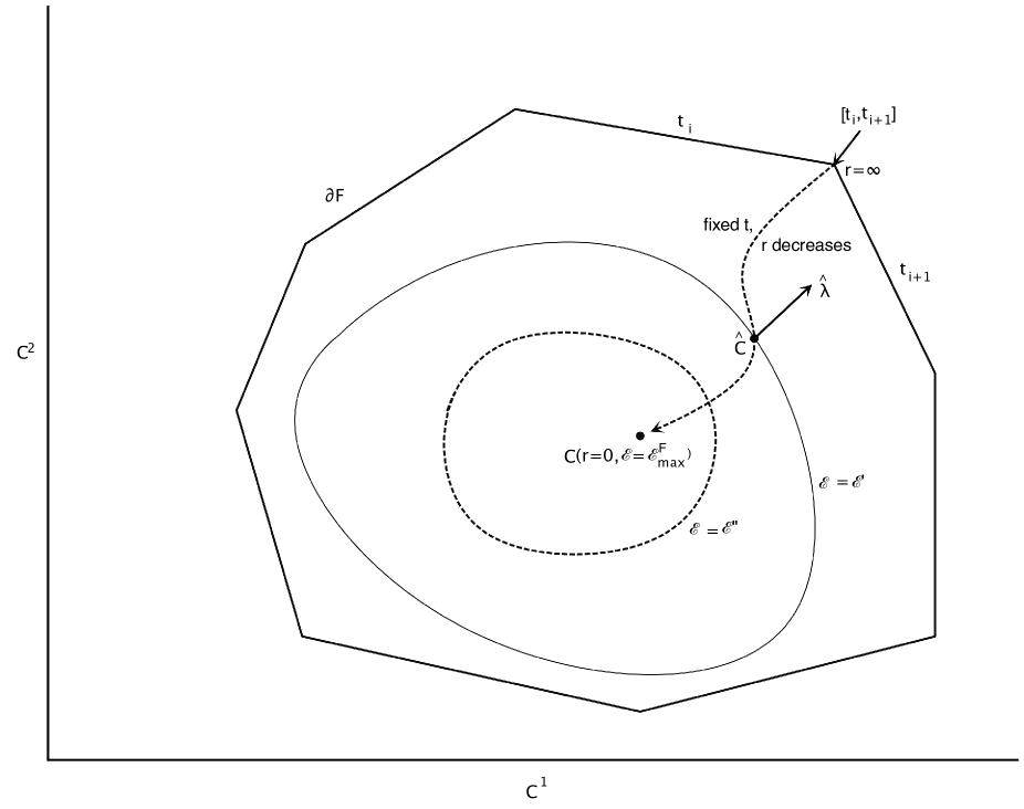
Figure 4: The covariogram and related objects

This is a convex polyhedron, which we call the covariogram. It includes the observed commoments $\hat{\bm{C}}$, as well as the vector of moments $C^{\bm{\lambda}}$ generated by the optimal matching $\bm{\mu}^{\bm{\lambda}}$ for any value of the parameter vector $\bm{\lambda}$. Each feasible matching $\bm{\mu}$ also has a generalized entropy $\mathcal{E}(\bm{\mu},\bm{\hat{r}})$; we denote $\mathcal{E}^{\bm{\lambda}}\equiv\mathcal{E}(\bm{\mu}^{\bm{\lambda}},\bm{\hat{r}})$ the generalized entropy associated with parameter vector $\bm{\lambda}$. Since the vectors $\phi$ are linearly independent, the mapping $\bm{\lambda}\longrightarrow C^{\bm{\lambda}}$ is invertible on the covariogram. Denote $\bm{\lambda}(C)$ its inverse. The corresponding optimal matching has generalized entropy $\mathcal{E}_{r}\left(C\right)=\mathcal{E}^{\bm{\lambda}\left(C\right)}$. The level sets of the function $\mathcal{E}_{r}$ are isoentropy surfaces in the covariogram.

Figure 4 illustrates these concepts. It assumes $K=2$ basis functions, so that the covariogram is a convex polyhedron in $(C^{1},C^{2})$ plane. Since $\bm{\lambda}$ also is two-dimensional, it can be represented in polar coordinates. Let the data be generated by $\bm{\lambda}=r\exp(it)$. For $r=0$, the model is uninformative: matching is random and generalized entropy takes its maximum possible value $\mathcal{E}^{F}_{\mbox{max}}$ among all possible matchings. We denote $C_{0}$ the corresponding moments. At the other extreme, the boundary $\partial F$ of the covariogram corresponds to $r=\infty$. There is no unobserved heterogeneity; generically over $t$, the moments generated by $\bm{\lambda}$ must belong to a finite set of vertices, so that $\bm{\lambda}$ is only set-identified.

As $r$ decreases for a given $t$, the corresponding moments follow a trajectory indicated by the dashed line on Figure 4, from the boundary $\partial F$ to the point $C_{0}$. The entropy $\mathcal{E}^{\bm{\lambda}}$ increases as this trajectory crosses contours of higher entropy ($\mathcal{E}^{\prime}$ then $\mathcal{E}^{\prime\prime}$ on the figure.)

We know from Theorem 6.2 that the moment-matching estimator $\hat{\bm{\lambda}}^{MM}$ is the vector of multipliers of the program that maximizes entropy over the matchings that generate the observed values of the moments. Therefore $\partial\mathcal{E}_{r}(\hat{C})/\partial C^{k}=\hat{\lambda}_{k}^{MM}$; and the moment-matching estimator lies on the normal to the isoentropy contour that goes through the observed moments $\bm{\hat{C}}$. This is shown as $\hat{\lambda}$ on Figure 4.

E.3 Parameterization, testing, and multimarket data

Proposition 4 shows that, given a specification of the distribution of the unobserved heterogeneities $\bm{P}_{x}$ and $\bm{Q}_{y}$, there is a one-to-one correspondence between $\bm{\mu}$ and $\bm{\Phi}$. To put it differently: any matching on a single market can be rationalized by exactly one model that satisfies Assumptions 1 and 2, for any such vector of distributions. This has several consequences for analysts using data on a single market. Without further restrictions, it is impossible to test separability, even assuming perfect knowledge of the distributions of unobserved heterogeneity. It is also impossible to discriminate between separable models based on different distributions. One way out of this conundrum is to incorporate credible restrictions (inspired by theoretical restrictions, or by institutional features of the market) into both the surplus matrix $\bm{\Phi}$ and the distributions of unobservable heterogeneity $\bm{P}_{x}$ and $\bm{Q}_{y}$. To take a simple example, suppose that we know that there is no interaction between partner characteristics $x^{k}$ and $y^{l}$ in the production of joint surplus: for fixed values of the other characteristics, $\Phi_{xy}$ is additive in $x^{k}$ and $y^{l}$. Given our identification formula (3.9) and observed matching patterns, this translates into a set of constraints on the derivatives of the generalized entropy, and therefore on the distributions $\bm{P}_{x}$ and $\bm{Q}_{y}$. Adding constraints on the distributions would make the model testable. As another example, consider a semiparametric specification in the spirit of Ekeland, Heckman, and Nesheim (2004): $\Phi_{xy}=\bm{b}_{y}^{\prime}\bm{\phi}_{x}$, with known $d$-dimensional vectors $\bm{\phi}_{x}$ and unknown vectors $\bm{b}_{y}$. If $d<\lvert Y\rvert$, this would restrict the number of degrees of freedom in $\bm{\Phi}$, freeing parameters to specify the distributions of heterogeneity and/or to test the model. An alternative empirical strategy is to use multiple markets with restricted parametric variation in the joint surplus $\bm{\Phi}$ and the distributions of unobserved heterogeneity $\bm{P}_{x}$ and $\bm{Q}_{y}$. The variations in the group sizes $\bm{n}$ and $\bm{m}$ across markets then generate variation in optimal matchings that can be used to overidentify the model and generate testable restrictions. Chiappori, Salanié, and Weiss (2017) relied on a variant of this approach.

Appendix F Computational Methods and Benchmarks [online]

Section 4 described two classes of methods to compute the equilibrium matching patterns: min-Emax, and IPFP. Min-Emax is more generally applicable than IPFP; on the other hand, IPFP is much faster. To document these claims, we present in this appendix a small simulation of the Choo and Siow model that explores the computational performance of four different methods: a general-purpose equation solver, the min-Emax method, the minimization of the function $F$ expressed in (3.14), and IPFP.

In the second part of this appendix, we show how linear programming techniques can be used to solve and estimate a model with discretized error distributions.

F.1 Benchmarks

We simulated ten cases, with a number of categories $|\mathcal{X}|=|\mathcal{Y}|$ that goes from 100 to 5,000. For each of these ten cases, we draw the $n_{x}$ and $m_{y}$ uniformly in $\{1,\ldots,100\}$; and for each $(x,y)$ match we draw $\Phi_{xy}/2$ from $\mathcal{N}(0,1).$

F.1.1 Minpack

We applied the Levenberg-Marquardt solver Minpack to the system of $(\mathcal{X}|+|\mathcal{Y})$ equations that characterizes the optimal matching (see Section 4). Minpack is probably the most-used solver in scientific applications; it underlies many statistical and numerical packages.

F.1.2 Min-Emax

The min-Emax method we described in Section 4 minimizes $\left(G(\bm{U},\bm{n})+H(\bm{\Phi}-\bm{U},\bm{m})\right)$ over the $|\mathcal{X}|\times|\mathcal{Y}|$ object $\bm{U}=(U_{xy}).$ In the particular case of the Choo and Siow model, the function $G$ is given by

$$G(\bm{U},\bm{n})=\sum_{x\in\mathcal{X}}n_{x}\log\left(1+\sum_{y\in\mathcal{Y}}\exp(U_{xy})\right)$$

and $H$ has the same form.

We used the Knitro optimizer to obtain the solution.

F.1.3 Minimizing $F$

Formula (3.14) provides us with an alternative method that works on the smaller object $(u_{x},v_{y})$ of group average utilities. Here again we used the Knitro optimizer.

F.1.4 IPFP

Consider the logit model of Choo and Siow.

Fix a value of $\bm{\lambda}$ and drop it from the notation: let the joint surplus function be $\bm{\Phi}$, with optimal matching $\bm{\mu}.$ Formula (3.12) can be rewritten as

$$\mu_{xy}=\exp\left(\frac{\Phi_{xy}}{2}\right)\sqrt{\mu_{x0}\mu_{0y}}.$$ (F.1)

As noted by Decker, Lieb, McCann, and Stephens (2012) we could just plug this into the feasibility constraints $\sum_{y}\mu_{xy}+\mu_{x0}=n_{x}$ and $\sum_{x}\mu_{xy}+\mu_{0y}=m_{y}$ and solve for the masses of singles $\mu_{x0}$ and $\mu_{0y}.$ This results in a system of $\lvert\mathcal{X}\rvert+\lvert\mathcal{Y}\rvert$ equations:

$$\mu_{x0}+\left(\sum_{y\in\mathcal{Y}}\exp\left(\frac{\Phi_{xy}}{2}\right)\sqrt{\mu_{0y}}\right)\sqrt{\mu_{x0}} =n_{x}$$ (F.2)

$$\mu_{0y}+\left(\sum_{x\in\mathcal{X}}\exp\left(\frac{\Phi_{xy}}{2}\right)\sqrt{\mu_{x0}}\right)\sqrt{\mu_{0y}} =m_{y}.$$ (F.3)

Taking the unknowns to be $\sqrt{\mu_{x0}}$ and $\sqrt{\mu_{0y}}$, each of these equations is quadratic in the unknowns. IPFP simply consists of solving the system (F.2) iteratively. Starting from an arbitrary guess $\mu_{0y}^{(0)}$, at step $(2k+1)$ we find the following updating equation (4.2). These equations are easily solved in closed form. The pseudo-code in Algorithm 1 gives a detailed implementation.  Note that since in the Choo and Siow model the shadow prices $u_{x}$ and $v_{y}$ are simply minus the logarithms of the corresponding $\mu_{x0}$ and $\mu_{0y}$, this algorithm in fact operates on $u_{x}$ and $v_{y}$.

Algorithm 1.

Solving for the optimal matching by IPFP

two non-negative vectors $\bm{n}$ and $\bm{m}$ (sizes $M$ and $N$); a matrix $\bm{\Phi}$ of size $(M,N)$

a tolerance $\tau$ and a maximum number of iterations $I$

the matrix $\bm{\mu}$ of size $(M,N)$ holds the marriage patterns at the optimal matching

$X\leftarrow\mbox{size}(\bm{n})$

$Y\leftarrow\mbox{size}(\bm{m})$

$\bm{K}\leftarrow\exp(\bm{\Phi}/2)$

$\delta\leftarrow\infty,i\leftarrow 0$

$\bm{T}\leftarrow 0_{Y}$

while $\delta>\tau$ and $i<I$ do

     $\bm{S}\leftarrow\bm{K}\bm{T}$ $\triangleright$ Project on $\bm{n}$ margins

     $\bm{t}\leftarrow\left(\sqrt{\bm{S}^{2}+4\bm{n}}-\bm{S}\right)/2$

     $S\leftarrow\bm{K}^{\prime}\bm{t}$ $\triangleright$ Project on $\bm{m}$ margins

     $\bm{T}\leftarrow\left(\sqrt{\bm{S}^{2}+4\bm{m}}-\bm{S}\right)/2$

     $\delta_{1}\leftarrow\max\;\lvert\bm{t}^{2}+\bm{t}\odot\bm{K}\bm{T}-\bm{n}\rvert$ $\triangleright$ Error on $\bm{n}$ margins

     $\delta_{2}\leftarrow\max\;\lvert\bm{T}^{2}+\bm{T}\odot\bm{K}^{\prime}\bm{t}-\bm{m}\rvert$ $\triangleright$ Error on $\bm{m}$ margins

     $\delta\leftarrow\max(\delta_{1},\delta_{2})$

     $i\Leftarrow i+1$

end while

if $i\geq I$ then

     Failed to achieve requested precision

else

     $\bm{\mu}\leftarrow\bm{K}\odot(\bm{t}\otimes\bm{T})$ $\triangleright$ $\otimes$ denotes outer product and $\odot$ element-wise product

end if

F.1.5 Results

For all four methods, we used C/C++ programs run on a single processor of a Mac desktop. We set the convergence criterion for all methods as a relative estimated error of $10^{-6}.$ This is not as straightforward as one would like: both Knitro and Minpack rescale the problem before solving it, while we did not attempt to do it for IPFP. Still, varying the tolerance within reasonable bounds hardly changes the results, which we present in Figure 5. Each panel gives the distribution of CPU times for one of the four methods, in the form of a Tukey box-and-whiskers graph.

There are three things to note about these graphs. First, distances on the $x$-axis are not drawn to scale, except for the smaller number of categories; second the $y$-axis is logarithmic; third, for some methods we only report results on the lower range of categories. The reasons are obvious from the graphs. Minpack solving not scale up well. The min-Emax method that minimizes $(G(\bm{U})+H(\bm{\Phi}-\bm{U}))$ is even worse: in this “logit” case, it is not competitive beyond 100 categories as it minimizes in a high-dimensional space. On the other hand, the min-Emax method that optimizes over $\bm{u}$ and $\bm{v}$ and the IPFP algorithm both perform remarkably well, even with several thousands of categories.

Choo and Siow only used 60 categories in their application (ages from 16 to 75). For such numbers, all four methods work well, but IPFP and min-Emax on $(u,v)$ again clearly dominate. We should emphasize that only the special structure of the Choo and Siow model allowed us to reduce the dimensionality by minimizing over $\bm{u}$ and $\bm{v}$. IPFP, on the other hand, can be used in a broader class of models. While IPFP has more variability than the other methods (perhaps because we did not rescale the problem beforehand), even the slowest convergence times for each problem size are at least three times smaller than those of Minpack. This is all the more remarkable that IPFP does not require any calculation of derivatives; by comparison, we fed the code for the Jacobian of the system of equations into Minpack. IPFP also compares very well with the min-Emax method on $(u,v)$, even though we fed the Jacobian and the Hessian into Knitro.

Finally, while we have run these experiments on a single processor, it is clear that IPFP is much more amenable to parallel implementation than the optimization methods, since each iteration solves $|\mathcal{X}|$ or $|\mathcal{Y}|$ equations that are independent of each other.

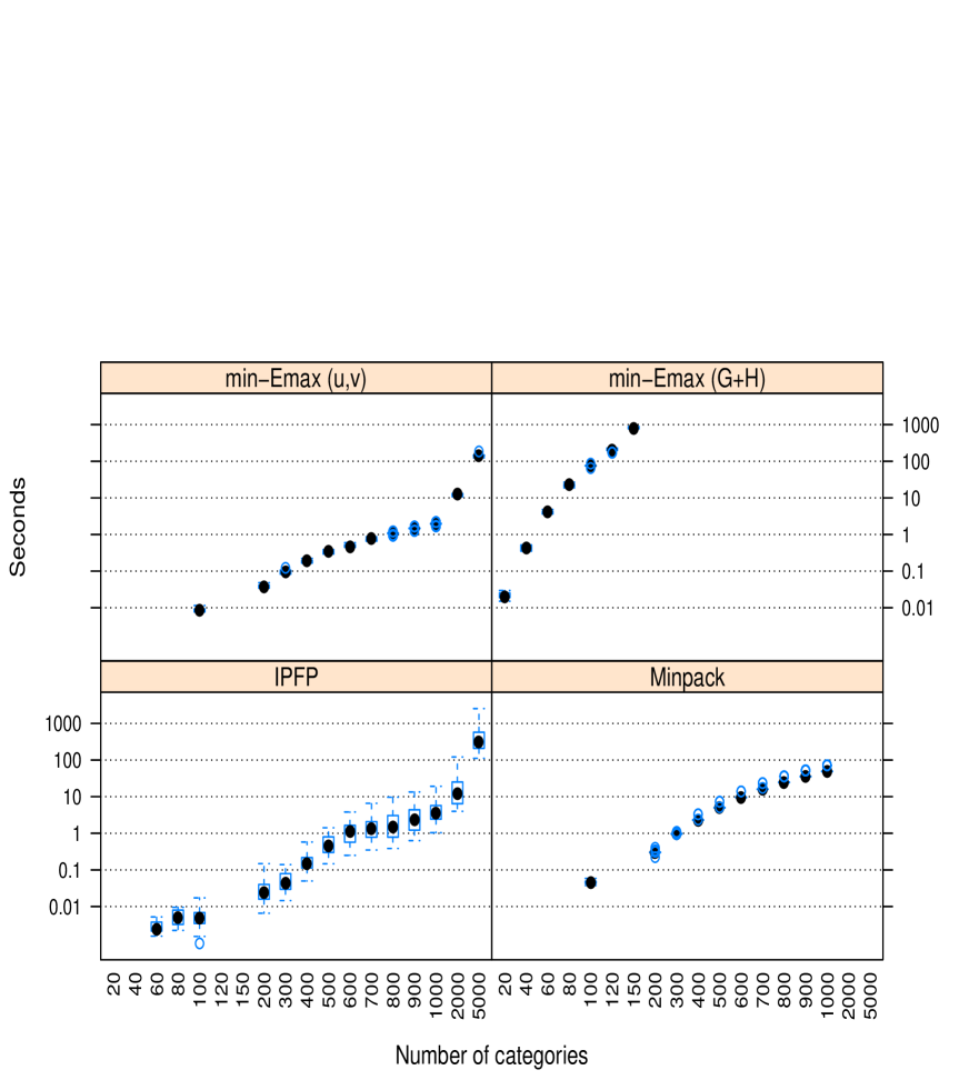
Figure 5: Solving for the optimal matching

F.2 An additional method: linear programming

Min-Emax and IPFP both exploit the structure of the separable matching problem. A more “brute-force” alternative is to simply solve the underlying linear programming problem. This requires discretizing the distribution of the error terms. We now explain how it can be done, and we extend it to obtain the moment-based estimator in a semilinear model.

F.2.1 Equilibrium via linear programming

Now suppose that the vectors $\varepsilon$ and $\eta$, instead of having full support, only take a finite number of values: these are analogous to the unobserved “types” of many structural econometric models. We define $(\varepsilon_{y}^{xk})_{y\in\mathcal{Y}_{0},k=1,\ldots,K_{x}}$ to be the points of support of $\mathbf{P}_{x}$, and $(r_{x}^{k})$ their probabilities; and we define $(\eta_{x}^{yl})$ and $(s^{l}_{y})$ similarly. In this case, $G(\bm{U},\bm{n})$ is $\sum_{x}n_{x}E_{\mathbf{P}_{x}}\max_{y}(U_{xy}+\varepsilon_{y})$, that is

$$G(\bm{U},\bm{n})=\sum_{x\in\mathcal{X}}n_{x}\sum_{k=1}^{K_{x}}r^{k}_{x}\max\left(\varepsilon_{0}^{xk},\max_{y\in\mathcal{Y}}(U_{xy}+\varepsilon_{y}^{xk})\right).$$

Define $u_{x}^{k}=\max\left(\varepsilon_{0}^{xk},\max_{y\in\mathcal{Y}}(U_{xy}+\varepsilon_{y}^{xk})\right)$, and $v_{y}^{l}=\max\left(\eta_{0}^{yl},\max_{x\in\mathcal{X}}(V_{xy}+\eta_{x}^{yl})\right)$. By construction,

$$u_{x}^{k} \geq U_{xy}+\varepsilon_{y}^{xk}\;\;\forall y\;\;\mbox{ and }\;u_{x}^{k}\geq\varepsilon_{0}^{xk}$$ (F.4)

$$v_{y}^{l} \geq V_{xy}+\eta_{x}^{yl}\;\;\forall x\;\;\mbox{ and }\;v_{y}^{l}\geq\eta_{0}^{yl}.$$ (F.5)

It follows from (3.6) that we minimize the objective function and given the constraint $U_{xy}+V_{xy}\geq\Phi_{xy}$, it is easy to see that the optimal matching solves

$$\mathcal{W}(\bm{\Phi},\bm{n},\bm{m})=\min_{\bm{u},\bm{v},\bm{U}}\left(\sum_{x\in\mathcal{X}}n_{x}\sum_{k=1}^{K_{x}}r^{k}_{x}u^{k}_{x}+\sum_{y\in\mathcal{Y}}m_{y}\sum_{l=1}^{L_{y}}s^{l}_{y}v_{y}^{l}\right)$$

subject to the constraints (F.4) and (F.5) with $V_{xy}=\Phi_{xy}-U_{xy}.$ Note that the objective function and the constraints are linear in the variables. Therefore solving for equilibrium with finite types boils down to a linear programming problem, for which very fast algorithms are available (even with many variables). The multipliers of the constraints at the optimum give the matching patterns for each type in each group, and can be averaged over types to yield the $\mu_{xy}$. This idea can be taken further: any distributions $\mathbf{P}_{x}$ and $\mathbf{Q}_{y}$ can be discretized. Solving the program above for a given finite-support approximation of the distributions gives an approximation that can be shown to converge to the optimum for the limit of the discrete distributions, by adapting an argument of Chernozhukov, Galichon, Hallin, and Henry (2017, Theorem 3.1). Hence the approach described in this subsection is applicable to any separable model.

F.2.2 Computing the moment-matching estimator

The linear programming approach of Subsection F.2.1 can be extended in order to compute the moment-matching estimator in the semilinear models of Section 5.2. Equation (5.4) shows that the moment-matching estimator minimizes $\min_{\bm{\lambda}}\left(\mathcal{W}(\bm{\lambda}^{\prime}\bm{\tilde{\phi}},\hat{\bm{r}})-\bm{\lambda}^{\prime}\hat{C}\right)$ over $\lambda$. This suggests a general approach to the estimation of separable models with known distributions of heterogeneity. First, specify a linear surplus function and distributions of unobservable heterogeneity $\mathcal{P}_{x}$ and $\mathcal{Q}_{y}$. Second, discretize the latter distributions. Third, solve the following linear program:

$$\min_{\bm{u},\bm{v},\bm{U},\bm{\lambda}}\left(\sum_{x\in\mathcal{X}}\hat{n}_{x}\sum_{k=1}^{K_{x}}r_{x}^{k}u_{x}^{k}+\sum_{y\in\mathcal{Y}}\hat{m}_{y}\sum_{l=1}^{L_{y}}s_{y}^{l}v_{y}^{l}-\bm{\lambda}^{\prime}\hat{C}\right)$$

under the constraints (F.4) and (F.5), replacing $V_{xy}$ with $\bm{\lambda}^{\prime}\bm{\tilde{\phi}_{xy}}-U_{xy}$. The objective and the constraints are still linear with respect to all variables, which now also include $\bm{\lambda}$. Once again, this program can be solved efficiently by linear programming algorithms, yielding both the moment-matching estimator and the corresponding average utilities and matching patterns.

A summary

Each computational method has pros and cons. The min-Emax method can be applied quite generally. It requires many evaluations of $G$ and $H$ however, which may be costly for large $|\mathcal{X}|,|\mathcal{Y}|$. Linear programming is attractive in semilinear models, at the price of discretization. IPFP requires no discretization, provides easy estimation of linear model, and is highly scalable. It does require evaluating the extended entropy $E$ of Section A.7, which is straightforward in logit-type models.

Appendix G Application to Choo and Siow’s data [online]

Our empirical application uses the data Choo and Siow (2006) put together, with some minor changes. We also put more emphasis on the treatment of those $(x,y)$ cells that have zero observations.

G.1 The data

Choo and Siow used data from the Census to evaluate the numbers $\bm{n}$ and $\bm{m}$ of men and women of every age in every state; and they relied on National Center for Health Statistics data to estimate the number of marriages by state and by age cell. They were kind enough to share with us their samples and programs; the description that follows is very similar to that in their paper, and in fact quotes freely from it.

G.1.1 The populations

Data on the populations of men and women of every age and state were extracted from the Integrated Public-Use Microdata Sample files of the U.S. Census (see Ruggles, Genadek, Goeken, Grover, and Sobek, 2015). Choo and Siow used data from the 1970 and 1980 U.S. Census to construct population vectors:

The samples used were the 5 percent state samples for 1980 and the 1 percent Form 1 and Form 2 samples for 1970. The 1970 data sets were appropriately scaled to be comparable with the 1980 files.

[…]

We use the marst variable in the census to identify a person as either never married, currently married, or previously married (divorced or widowed). To calculate the number of available individuals, we simply add the never marrieds and previously married.

Choo and Siow kept all individuals aged 16 to 75. Since the number of first marriages in which either partner is older than 40 is rather small in the 70s and 80s, we decided to focus on the populations aged 16 to 40 instead. The “state” of an individal is defined as his/her place of residence.

G.1.2 The marriages

Choo and Siow obtained data on marriages from the Vital Statistics reports that many states send to the National Center for Health Statistics (NCHS):

Marriage records from the 1971/72 and 1981/82 Vital Statistics were used to construct the bivariate distributions of marriages. A state has to report the number of marriages to the National Center for Health Statistics to be in the sample.

We deviated from their paper in two respects.

• To be consistent with our age window for populations in the basis year we only keep marriages in which either partner is at most 41 (in the Census year+1) or 42 (in the Census year+2). We corrected a small mistake in the construction of the data—Choo and Siow (2006) did not update the ages of the subjects between Census year+1 and Census year+2. This does not affect their main conclusions.

• The list of states we include in our application is slightly different. They excluded Iowa, Minnesota, and South Carolina which we do use since they reporteed to the NCHS in both waves. Colorado only reported to the NCHS after 1980. Choo and Siow excluded it from their study; we keep it in the 1980s wave. Choo and Siow also excluded New York City from New York State. We eventually decided to exclude both.

A “reform” state is one in which the Roe v. Wade Supreme Court decision affected the legal status of abortion. Our list of reform states comprises Alaska, California, Delaware, Florida, Georgia, Hawaii, Kansas, Maryland, and (in the 1980s only) Colorado. Our non-reform states are Alabama, Connecticut, Idaho, Illinois, Indiana, Iowa, Kentucky, Louisiana, Maine, Massachusetts, Michigan, Mississippi, Missouri, Montana, Nebraska, New Hampshire, New Jersey, Ohio, Pennsylvania, Rhode Island, South Dakota, Tennessee, Utah, Vermont, West Virginia, Wyoming, and the District of Columbia. We exclude from our study Arizona, Arkansas, Nevada, New Mexico, New York, North Dakota, Oklahoma, Texas, Washington, and (in the 1970s) Colorado.

G.1.3 Merging availables and marriages

Table 1 describes our data on the populations of men and women. The numbers between parenthesis refer to the population, the other numbers to the sample. With a total of $2.19$m observations representing $58.67$m individuals, our universe of men and women is about 40% smaller than Choo and Siow’s. This is a direct consequence of our focus on younger ages. The reform states have $34.6$% of the population in 1970 and $37.9$% in 1980. The sample is much larger in 1980, as the ACS dataset we use had a better sampling rate then.

Census		1970	1980	Population increase
Reform states	Men	$81,260$ ($4.32$m)	$351,231$ ($7.20$m)	$66.7$%
	Women	$66,920$ ($3.63$m)	$308,808$ ($6.37$m)	$76.2$%
Non-reform states	Men	$150,887$ ($7.82$m)	$566,460$ ($11.51$m)	$47.2$%
	Women	$137,839$ ($7.16$m)	$524,741$ ($10.68$m)	$49.2$%
Total	Men	$232,147$ ($12.14$m)	$917,691$ ($18.71$m)	$54.2$%
	Women	$204,759$ ($10.77$m)	$833,549$ ($17.05$m)	$58.3$%

Table 1: Numbers of men and women

Table 2 describes our subsample from the NCHS dataset. In this table $(rt,N)$ for instance refers to marriages in which the husband lists a reform state as his residence, and the wife lists a non-reform state. In more than 95% of marriages, husband and wife list a state with the same “reform status”. This is not surprising since a large majority of marriages in fact unite partners from the same state. As in Choo and Siow, the number of marriages increased much more in reform states than in non-reform states; but also less than the general population.

Wave	1971–72	1981–82	Population increase
(r,R)	$138,483$ ($838,140$)	$424,416$ ($1.00$m)	$19.4$%
(r,N)	$5,866$ ($38,518$)	$10,383$ ($32,952$)	$-14.5$%
(n,R)	$6,108$ ($33,440$)	$10,182$ ($24,530$)	$-26.6$%
(n,N)	$216,428$ ($1.70$m)	$506,953$ ($1.79$m)	$4.9$%
Total	$366,885$ ($2.61$m)	$951,934$ ($2.84$m)	$8.9$%

Table 2: Numbers of marriages

Finally, Table 3 shows that the average age at marriage increased by two years, quite uniformly across reform status and genders. As a consequence, the age difference also did not change, with husbands two years older than their wives.

Wave		1971–72	1981–82	Increase
Reform states	Men	$23.0$	$25.1$	$2.1$
	Women	$20.9$	$23.0$	$2.1$
Non-reform states	Men	$22.7$	$24.7$	$2.0$
	Women	$20.6$	$22.6$	$2.0$

Table 3: Ages at marriage

G.2 Zero cells

Like much discrete-valued economic data, the Choo and Siow data contains a small but non-negligible percentage of $(x,y)$ cells with no observed match—up to 3%, depending on the subsample. The CS specification by construction rules out zero probability cells, and Choo and Siow (2006, footnote 15, p. 186) used kernel smoothers to impute positive probabilities in these “zero cells”. More generally, no separable model with full support can simulate zero cells (see our discussion of Assumption 2).

This is not an issue with unrestricted estimation, since we only need to assign a value of $-\infty$ to the corresponding $\Phi_{xy}$. With parametric inference, maintaining Assumption 2 implies that the model is misspecified. This is a minor consideration in practice, as the estimated probabilities of these cells turn out to be very small. A cleaner alternative is to specify error distributions $\bm{P}_{x}$ and $\bm{Q}_{y}$ that do not have full support, either because their supports have lower dimension and/or because their supports are bounded.

G.3 Detailed Estimation Results

G.3.1 Selecting Basis Functions

We used our moment matching method to estimate 625 semilinear versions of the original Choo and Siow (2006) specification, which we will call “the homoskedastic logit model”. They all include the two basis functions $\phi^{1}_{xy}\equiv 1$ and $\phi^{2}_{xy}=D_{xy}\equiv\mathrm{1\kern-3.99994pt1}(x\geq y)$, where $x$ is the age of the husband and $y$ that of the wife—both linearly transformed to be in [-1,1]. The $D$ term accounts for possible jumps or kinks in surplus when the wife is older than the husband ($D=0$). In addition to these two basis functions, we include a varying set of functions of the form $x^{i}y^{j}$ and $x^{i}y^{j}D$. Our richest candidate specification has 98 basis functions; note that the nonparametric model has 625 (as many as marriage cells.)

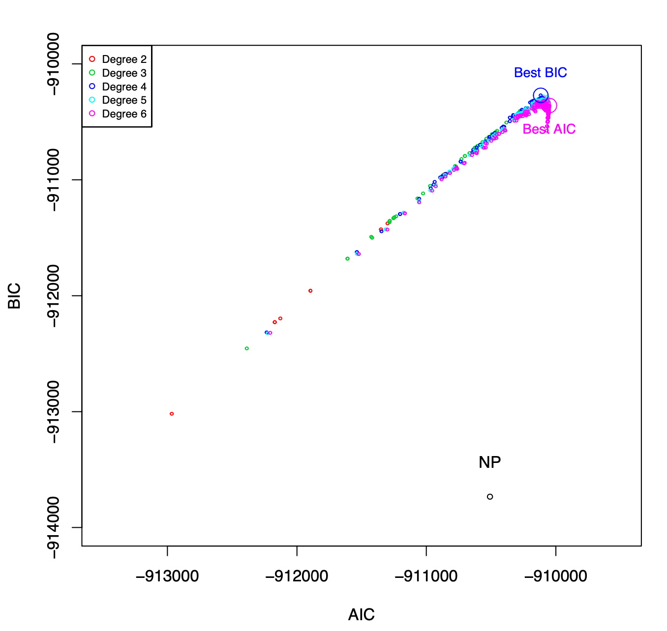
Figure 6: AIC and BIC Values for the Parametric and Nonparametric Choo and Siow Models

Figure 6 plots the values of the Akaike Information Criterion (on the horizontal axis) and of the Bayesian Information Criterion (on the vertical axis) for the 625 models, and for the nonparametric model NP. The location of NP shows that even for our sample of a couple hundred thousand observations, it is severely overparameterized: no fewer than 490 of our 625 models have a better AIC, and all of them have a better BIC.

Our best AIC model is still large: it has 60 coefficients, of which 49 are significant at 5%. With such a large sample, we could probably have included even higher-degree terms and improved the AIC slightly. While the AIC criterion subtracts twice the number of parameters from the log-likelihood, the BIC criterion penalizes it by half of the logarithm of the number of observations. With our 224,068 observations, this amounts to $6.2$ rather than $2$ times the number of parameters. As a result, the BIC-selected model only has 30 coefficients, of which 28 differ significantly from 0 at the 5% level. For model selection (as opposed to forecasting), BIC is more appropriate than AIC and we will work with its 30 selected basis functions from now on: all terms $x^{m}y^{n}$ and $x^{m}y^{n}D$ for $1\leq m\leq 2$ and $1\leq n\leq 4$.

G.3.2 The Homoskedastic Choo and Siow Model

Table 4 gives the estimated coefficients and their bootstrapped standard errors and Students for the BIC-preferred modelin this class.

	Estimates	Standard Errors	Students
$1$	-11.163	0.023	-490.9
$D$	1.147	0.066	17.3
$X$	-14.759	0.336	-44.0
$XD$	5.204	0.134	38.7
$X^{2}$	-13.211	0.208	-63.4
$X^{2}D$	5.656	0.104	54.2
$Y$	-1.220	0.066	-18.4
$YD$	4.757	0.127	37.5
$Y^{2}$	-2.064	0.041	-50.7
$Y^{2}D$	5.950	0.118	50.5
$Y^{3}$	1.097	0.054	20.4
$Y^{3}D$	1.659	0.029	57.4
$Y^{4}$	-0.563	0.033	-17.0
$Y^{4}D$	-0.637	0.018	-35.5
$XY$	26.379	0.403	65.4
$XYD$	-16.697	0.336	-49.7
$XY^{2}$	-16.956	0.455	-37.3
$XY^{2}D$	10.238	0.298	34.3
$XY^{3}$	6.206	0.336	18.4
$XY^{3}D$	-3.936	0.227	-17.3
$XY^{4}$	-0.997	0.144	-6.9
$XY^{4}D$	0.881	0.092	9.6
$X^{2}Y$	12.940	0.276	46.9
$X^{2}YD$	-11.549	0.226	-51.1
$X^{2}Y^{2}$	-5.636	0.303	-18.6
$X^{2}Y^{2}D$	4.938	0.229	21.5
$X^{2}Y^{3}$	1.131	0.196	5.8
$X^{2}Y^{3}D$	-1.053	0.137	-7.7
$X^{2}Y^{4}$	0.085	0.060	1.4
$X^{2}Y^{4}D$	-0.072	0.050	-1.4

Table 4: Estimates for the Homoskedastic Logit Model

Estimates

Table 4 in Appendix G.3 collects our estimates for the coefficients of the BIC-preferred model with iid standard type I EV errors. Since the distributions $\mathbb{P}_{x}$ and $\mathbb{Q}_{y}$ are parameter-free in this model, the table shows the estimated coefficients for the 30 basis functions in its first column. We evaluated their standard errors (third column) with a bootstrap procedure based on 999 draws from the estimated variance-covariance matrix of the observed matching patterns $\bm{\hat{\mu}}$.

The bootstrap also allows us to compute a $p$-value for the entropy test described in Theorem 6. The value of the entropy test statistic in the sample has a bootstrapped $p$-value is $0.856$. Recall that this tests the hypothesis that the true surplus function is a linear combination of our 30 basis functions, conditional on the distributional assumptions being true. The $p$-value tells us that this “spanning hypothesis” would only be rejected at the 15% level. This confirms that the 30-bases model is a very good approximation to the data-generating process. The Choo and Siow model aims at explaining marriage patterns by age, from age 16 to age 75. In the early 1970s, close to 80% of marriages occurred before either partner was 30 years old, so that the number of data points to fit is rather small. Even using BIC to reward parsimony, with more than 200,000 observations we end up with a rich model and an excellent fit.

As a consequence, the distributional parameters we introduce can only improve the fit marginally. We did find, however, that allowing for gender- and age-dependent heteroskedasticity yielded a notable improvement in the fit. Interestingly, it also changes the profile of surplus-sharing within couples: the share that goes to the husband increases much more steeply than in the original (homoskedastic) Choo and Siow specification. We also fitted several Generalized Extreme Values models. The most promising ones seem to be those of the FC-MNL family (Davis and Schiraldi, 2014), which incorporate the type of local correlation patterns that are missing from the multinomial logit framework. While they do not outperform the basic Choo and Siow specification in our application, they are easy to implement and seem to us to have much potential in matching models.

Heteroskedastic Logit Models

We explored several ways of adding heteroskedasticity to the benchmark model. It is clear from 1.2 that the parameters can only be identified up to a scale normalization: multiplying both $\bm{\Phi}$ and the error terms $\bm{\varepsilon}$ and $\bm{\eta}$ by the same positive number has no effect on the equilibrium matching. The Choo and Siow (2006) model normalizes the scale (twice) by using standard type I EV errors for both $\bm{\varepsilon}$ and $\bm{\eta}$. When adding heteroskedasticity to $\bm{\varepsilon}$ and $\bm{\eta}$, we need to maintain one normalization.

Our simplest heteroskedastic model still uses a standard type I EV $\bm{\varepsilon}$ (our scale normalization) and adds only one parameter $\tau$, with

$$\tau^{2}=\frac{V\eta}{V\varepsilon}.$$

This model allows for heteroskedasticity across genders, but not across types. Somewhat surprisingly, the profiled loglikelihood of the model is very flat with respect to $\tau$. While we did obtain an estimate of $0.927$ that is slightly lower than one, the improvement in the loglikelihood is so small that the values of both AIC and BIC deteriorate.

Going further, we allow for type- and gender-dependent heteroskedasticity. To do this, we multiply the terms $\bm{\varepsilon}_{i\cdot}$ (resp. $\bm{\eta}_{j\cdot}$) by scale factors $\sigma_{x}$ (resp. $\tau_{y}$). We experimented with specifications of the form

$$\sigma_{x} =\exp(\sigma_{1}x+\ldots+\sigma_{p}x^{p})$$

$$\tau_{y} =\exp(\tau_{0}+\tau_{1}y+\ldots+\tau_{q}y^{q})$$

Note that we do not allow for a constant term $\sigma_{0}$; this gives us the requisite scale normalization.

Of all such specifications for $0\leq p\leq 4$ and $1\leq q\leq 4$, this yields the largest improvement in the fit: a sizeable $+38.5$ points of loglikelihood, and $+25.2$ points on BIC. The estimates of the parameters of $\sigma_{x}$ and $\tau_{y}$ can be found in Table 5.

	Estimates	Standard Errors	Students
$\sigma_{1}$	0.793	0.051	15.4
$\tau_{0}$	-0.751	0.161	-4.7

Table 5: Estimates for the Heteroskedastic Logit Model: Distributional Parameters

Two-level, Two-nest Nested Logit

We estimated a two-level nested logit model in which we separate the singlehood option from all others. This model has two nests: one corresponding to singlehood, and one to the 25 possible ages of the partner. It introduces two additional parameters, $\gamma_{m}$ on the men side and $\gamma_{w}$ for women. The familiar equation from Choo and Siow (2006):

$$2\log\mu_{xy}=\log\mu_{x0}+\log\mu_{0y}+\Phi_{xy}$$

becomes

$$\gamma_{m}\log\frac{\mu_{xy}}{\sum_{t\in\mathcal{Y}}\mu_{xt}}+\gamma_{w}\log\frac{\mu_{xy}}{\sum_{z\in\mathcal{X}}\mu_{zy}}=\log\frac{\mu_{x0}}{\sum_{t\in\mathcal{Y}}\mu_{xt}}+\log\frac{\mu_{0y}}{\sum_{z\in\mathcal{X}}\mu_{zy}}+\Phi_{xy}.$$

The values of $(1-\gamma_{m})$ and $(1-\gamma_{w})$ can be interpreted as “within-nest correlations”; they equal zero in the Choo and Siow (2006) model.

We chose this specific nested logit model because we showed in Galichon and Salanié (2019) that it satisfies a “weak IIA” property–and we conjectured that it is the only separable model that does. When we tried to estimate this two-nest specification, we consistently found a corner maximum at $\gamma_{m}=1$. The other parameter $\gamma_{w}$ has a weak maximum at $0.91$, and the loglikelihood barely improves.

FC-MNL

Davis and Schiraldi (2014) show that for any admissible values of $\sigma$ and $\tau$, there exist values of the $b$ matrix that rationalize a given set of elasticities of substitution. We followed their suggestion of using $\sigma=0.5$ and $\tau=1.1$; and we chose the very parsimonious specification of the $b$ matrix described in Section 6.2. The maximum likelihood estimates for the distributional parameters are in Table 6.

	Estimates
$b_{m}(16)$	0.011
$b_{m}(40)$	0.000
$b_{w}(16)$	0.060
$b_{w}(40)$	0.000

Table 6: Estimates for the FC-MNL Model: Distributional Parameters

References

- (1)
- Agarwal (2015) Agarwal, N. (2015): “An Empirical Model of the Medical Match,” American Economic Review, 105, 1939–1978.
- Agarwal and Somaini (2020) Agarwal, N., and P. Somaini (2020): “Revealed Preference Analysis of School Choice Models,” Annual Review of Economics, 12, 471–501.
- Anderson, de Palma, and Thisse (1988) Anderson, S., A. de Palma, and J.-F. Thisse (1988): “A Representative Consumer Theory of the Logit Model,” International Economic Review, 29, 461–466.
- Arcidiacono and Miller (2011) Arcidiacono, P., and R. Miller (2011): “Conditional Choice Probability Estimation of Dynamic Discrete Choice Models With Unobserved Heterogeneity,” Econometrica, 79, 1823–1867.
- Bajari and Fox (2013) Bajari, P., and J. Fox (2013): “Measuring the Efficiency of an FCC Spectrum Auction,” American Economic Journal: Microeconomics, 5, 100–146.
- Bauschke and Borwein (1997) Bauschke, H., and J. Borwein (1997): “Legendre Functions and the Method of Random Bregman Projections,” Journal of Convex Analysis, 4, 27–67.
- Becker (1973) Becker, G. (1973): “A theory of marriage, part I,” Journal of Political Economy, 81, 813–846.
- Berry, Levinsohn, and Pakes (1995) Berry, S., J. Levinsohn, and A. Pakes (1995): “Automobile Prices in Market Equilibrium,” Econometrica, 63, 841–890.
- Berry and Pakes (2007) Berry, S., and A. Pakes (2007): “The Pure Characteristics Demand Model,” International Economic Review, 48, 1193–1225.
- Botticini and Siow (2011) Botticini, M., and A. Siow (2011): “Are there Increasing Returns in Marriage Markets?,” IGIER Working Paper 395.
- Boyd and Vandenberghe (2004) Boyd, S., and L. Vandenberghe (2004): Convex Oprtimization. Cambridge Universitry Press.
- Byrd, Nocedal, and Waltz (2006) Byrd, R., J. Nocedal, and R. Waltz (2006): “KNITRO: An Integrated Package for Nonlinear Optimization,” in Large-Scale Nonlinear Optimization, p. 35–59. Springer Verlag.
- Chernozhukov, Galichon, Hallin, and Henry (2017) Chernozhukov, V., A. Galichon, M. Hallin, and M. Henry (2017): “Monge-Kantorovich Depth, Quantiles, Ranks and Signs,” Annals of Statistics, 45, 223–256.
- Chiappori (2017) Chiappori, P.-A. (2017): Matching with Transfers: The Economics of Love and Marriage. Princeton University Press.
- Chiappori (2020) (2020): “The Theory and Empirics of the Marriage Market,” Annual Review of Economics, 12(1), 547–578.
- Chiappori, Galichon, and Salanié (2019) Chiappori, P.-A., A. Galichon, and B. Salanié (2019): “On Human Capital and Team Stability,” Journal of Human Capital, 13, 236–259.
- Chiappori, McCann, and Nesheim (2010) Chiappori, P.-A., R. McCann, and L. Nesheim (2010): “Hedonic Price Equilibria, Stable Matching, and Optimal Transport: Equivalence, Topology, and Uniqueness,” Economic Theory, 42, 317–354.
- Chiappori, Nguyen, and Salanié (2019) Chiappori, P.-A., D. L. Nguyen, and B. Salanié (2019): “Matching with Random Components: Simulations,” Columbia University mimeo.
- Chiappori and Salanié (2016) Chiappori, P.-A., and B. Salanié (2016): “The Econometrics of Matching Models,” Journal of Economic Literature, 54, 832–861.
- Chiappori, Salanié, and Weiss (2017) Chiappori, P.-A., B. Salanié, and Y. Weiss (2017): “Partner Choice, Investment in Children, and the Marital College Premium,” American Economic Review, 107, 2109–67.
- Chiong, Galichon, and Shum (2016) Chiong, K.-X., A. Galichon, and M. Shum (2016): “Duality in dynamic discrete-choice models,” Quantitative Economics, 7, 83–115.
- Choo and Siow (2006) Choo, E., and A. Siow (2006): “Who Marries Whom and Why,” Journal of Political Economy, 114, 175–201.
- Ciscato, Galichon, and Goussé (2020) Ciscato, E., A. Galichon, and M. Goussé (2020): “Like Attract Like: A Structural Comparison of Homogamy Across Same-Sex and Different-Sex Households,” Journal of Political Economy, 128, 740–781.
- Costinot and Vogel (2015) Costinot, A., and J. Vogel (2015): “Beyond Ricardo: Assignment Models in International Trade,” Annual Review of Economics, 7, 31–62.
- Csiszár (1975) Csiszár, I. (1975): “I-divergence Geometry of Probability Distributions and Minimization Problems,” Annals of Probability, 3, 146–158.
- Dagsvik (2000) Dagsvik, J. (2000): “Aggregation in Matching Markets,” International Economic Review, 41, 27–58.
- Daly and Zachary (1978) Daly, A., and S. Zachary (1978): “Improved Multiple Choice Models,” in Identifying and Measuring the Determinants of Mode Choice, ed. by D. Henscher, and Q. Dalvi. Teakfields, London.