Learning Slice-Aware Representations with Mixture of Attentions

Abstract

Real-world machine learning systems are achieving remarkable performance in terms of coarse-grained metrics like overall accuracy and F-1 score. However, model improvement and development often require fine-grained modeling on individual data subsets or slices, for instance, the data slices where the models have unsatisfactory results. In practice, it gives tangible values for developing such models that can pay extra attention to critical or interested slices while retaining the original overall performance. This work extends the recent slice-based learning (SBL) Chen et al. (2019) with a mixture of attentions (MoA) to learn slice-aware dual attentive representations. We empirically show that the MoA approach outperforms the baseline method as well as the original SBL approach on monitored slices with two natural language understanding (NLU) tasks.

⬇ def SF_Long(sentence,k=10): n = len(sentence .split(’ ’)) return n > k def SF_Question(sentence): return sentence[-1] == ’?’

Table 1: The designed slice functions (SFs). Left: We monitor three data slices - short utterances, those involving “time”, and those involving “email”. Right: We monitor long sentences and questions.

1 Introduction

Though machine learning systems have been achieving excellent performance in terms of coarse-grained metrics like accuracy, they perform poorly or even fail on some individual data subsets (i.e., slices). For instance, many models have difficulties when learning for classes with only a few samples or samples with challenging structures.

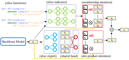
Figure 1: The slice-aware architecture with MoA. It consists of six components: (1) slice functions define the special data slices that we want to monitor; (2) backbone model for feature extraction (e.g., BERT); (3) slice indicators are membership functions to predict if a sample belongs to the slice; (4) slice experts aim to learn slice-specific representations; (5) shared head is the base task predictive layer across experts and (6) the proposed mixture of attentions (MoA) learns to attend to the slices of interest. It contains two different attention mechanism (red boxes): a membership attention and a dot-product attention. The MoA learns to re-weight the expert representation $\mathbf{r}$ to a slice-aware representation $\mathbf{s}$ and the original representation $\mathbf{x}$ to $\mathbf{s}$ (yellow lines). The slice distributions are computed in deterministic (weighted sum of slices) or stochastic (sampling) way in re-weighting $\mathbf{r}$ and $\mathbf{x}$.

Inspecting particular data slices can serve as an important component in model development cycles. A recently proposed slice-based learning (SBL) exhibited compelling results with more than 3% improvements on pre-defined slices Chen et al. (2019) in the task of binary classification. However, one potential limitation of the existing attention mechanism in SBL is that in multi-class cases, the attention suffers from the difficulty in using the experts’ confidences appropriately for computing slice distributions (refer to Sec. 3).

In this paper, we extend SBL with a mixture of attentions (MoA) mechanism. Two different attention mechanisms are learned to jointly attend to the defined slices from different representations in different latent subspaces. The first attention is based on slice membership likelihood and/or experts confidence as in SBL Chen et al. (2019), which we call membership attention. The second one is dot-product attention that is based on the backbone model (e.g., BERT Devlin et al. (2019)) extracted representations. The MoA approach is akin to multi-head attention Vaswani et al. (2017) but with different attention types that receive different inputs.

As presented in Figure 4, the two attentions in MoA can work jointly to attend to (1) the expert representation $\mathbf{r}$ and (2) the backbone model extracted representation $\mathbf{x}$, and finally form an attentive representation $\mathbf{s}$. The $\mathbf{s}$ is a slice-aware featurization of the samples in the particular data slices and will be used for making a final model prediction.

We argue that learning joint attention with MoA from different resources for computing slice distributions is beneficial Vaswani et al. (2017); Li et al. (2018). We evaluate the effectiveness of our proposed approach on intent detection Liu et al. (2019) and linguistic acceptability Warstadt et al. (2018) tasks.

Our main contributions are twofold:

• We extend SBL with MoA. The MoA approach has the ability to attend to slices in deterministic (weighted summation) and stochastic (sampling) ways.

• We conduct extensive experiments on two NLU tasks. The results show that MoA outperforms the baseline and vanilla SBL by average up to 9% and 6% respectively on defined slices.

2 Architecture

Figure 1 presents the slice-aware architecture based on SBL Chen et al. (2019). Let $\{x^{n},y^{n}\}_{n}^{N}$ be a dataset with N samples. We aim to learn slice-aware representation $\mathbf{s}$ from slice-experts-learned representation $\mathbf{r}$ and backbone-model-extracted representation $\mathbf{x}$.

We first define slice functions (SFs) as in Table 4 to split the dataset into $k$ slices of interests. Each sample is assigned with a slice label $\gamma\in[0,1]$ in $\{\gamma_{1},\gamma_{2},...,\gamma_{k}\}$ as supervision data.

Second, we use a backbone model like BERT to extract representation $\mathbf{x}\in\mathbf{R}^{d}$ for a given sample. Then, slice indicators $f_{i}(\mathbf{x};\mathbf{w}^{f}_{i})$, $\mathbf{w}^{f}_{i}\in\mathcal{R}^{d\times 1}$, $i\in\{1,..,k\}$ map $\mathbf{x}$ to a prediction $h_{i}$. $f_{i}$ are trained with $\{\mathbf{x}^{n},\gamma^{n}\}_{n}^{N}$ to predict whether a sample belongs to a particular slice. They are learned with cross entropy loss

$$\zeta_{1}=\sum_{i}^{k}\mathcal{L}_{CE}(h_{i},\gamma_{i})$$ (1)

Then, slice experts $g_{i}(\mathbf{x};\mathbf{w}^{g}_{i})$, $\mathbf{w}^{g}_{i}\in\mathcal{R}^{d\times d}$ learn a mapping from $\mathbf{x}$ to a slice vector $r_{i}\in\mathcal{R}^{d}$ with the samples that only belong to the slice, followed by a shared head, which is shared across all experts and maps $r_{i}$ to a prediction $\hat{y}=\varphi(r_{i};\mathbf{w}_{s})$. $g_{i}$ and $\varphi$ are learned on the base (original) task with ground-truth label $y$ by

$$\zeta_{2}=\sum_{i}^{k}\gamma_{i}\mathcal{L}_{CE}(\hat{y},y)$$ (2)

Finally, a mixture of attentions(MoA) (as in Sec. 3) re-weights $\mathbf{r}$ and $\mathbf{x}$ to form $\mathbf{s}$. The $\mathbf{s}$ goes through a final prediction function $\eta$ on the base task. The loss function is

$$\zeta_{3}=\mathcal{L}_{CE}(\eta(\mathbf{s};\mathbf{w}_{p}),y)$$ (3)

The total loss is a combination of the loss for slice indicators, slice experts and base task prediction function:

$$\zeta=\zeta_{1}+\zeta_{2}+\zeta_{3}$$ (4)

The whole model is optimised with back-propagation Rumelhart et al. (1986) in an end-to-end way.

3 Methodology

The SBL approach Chen et al. (2019) proposed a slice-residual attention modules (SRAMs) that are directly based on stacked membership likelihood $H\in\mathbf{R}^{k}$ and experts’ prediction confidence $\left|Y\right|\in\mathbf{R}^{c\times k}$, $c=1$ (i.e., binary classification). Then, slice distribution (attention weights) is computed with $a=\textsc{softmax}(H+\left|Y\right|)$. One potential limitation of this mechanism is that the above formulation can lead to mismatch shape in element-wise addition when $c>2$ (i.e., multi-class classification). To circumvent this, we propose a mixture of attentions (MoA) to augment membership attention with dot-product attention from different information resources.

3.1 Mixture of Attentions

Let $\mathbf{x}\in\mathbf{R}^{d}$ be the original representation from the backbone model (e.g., BERT), $h_{i}\in\mathbf{R}^{c}$ ($c=1$) as i-th indicator function’s prediction, and $r_{i}\in\mathbf{R}^{d}$ as i-th expert learned representation. When stacking on $k$ slices, we have $\mathbf{h}\in\mathbf{R}^{c\times k}$ and $\mathbf{r}\in\mathbf{R}^{d\times k}$. MoA’s goal is to (1) attend to $\mathbf{r}$ based on indicator functions’ membership likelihood and/or experts confidence; (2) attend to $\mathbf{x}$ with a dot-product attention; (3) to form a new slice-aware attentive representation $\mathbf{s}\in\mathbf{R}^{d}$ with weighted (sampled) $\mathbf{r}$ and $\mathbf{x}$.

The slice distributions are computed differently. For membership attention, the probability $\mathbf{p}_{1}=\textsc{softmax}(\mathbf{h})$ or $\mathbf{p}_{1}=\textsc{softmax}(\mathbf{h}+\left|\mathbf{r}\right|)\in\mathbf{R}^{k}$ ($d$=1 in binary classification). Then membership weighted slice representation is computed: $\mathbf{s}_{1}=\mathbf{r}\mathchoice{\mathbin{\vbox{\hbox{\scalebox{0.6}{$\displaystyle\bullet$}}}}}{\mathbin{\vbox{\hbox{\scalebox{0.6}{$\textstyle\bullet$}}}}}{\mathbin{\vbox{\hbox{\scalebox{0.6}{$\scriptstyle\bullet$}}}}}{\mathbin{\vbox{\hbox{\scalebox{0.6}{$\scriptscriptstyle\bullet$}}}}}\mathbf{p}_{1},\mathbf{s}_{1}\in\mathbf{R}^{d}$. For dot-product attention, we aim to learn an attention matrix $\mathbf{A}=\{\mathbf{a}_{1},...,\mathbf{a}_{k}\},\mathbf{a}\in\mathbf{R}^{d},\mathbf{A}\in\mathbf{R}^{d\times k}$ is randomly initialized and learned by the standard back-propagation. Intuitively, each $\mathbf{a}$ is learned to be a slice prototype Wang and Niepert (2019); Roy et al. (2020). The probability over slices is computed as:

$$\mathbf{p}_{2}=\textsc{softmax}(\mathbf{A}^{\top}\mathchoice{\mathbin{\vbox{\hbox{\scalebox{0.6}{$\displaystyle\bullet$}}}}}{\mathbin{\vbox{\hbox{\scalebox{0.6}{$\textstyle\bullet$}}}}}{\mathbin{\vbox{\hbox{\scalebox{0.6}{$\scriptstyle\bullet$}}}}}{\mathbin{\vbox{\hbox{\scalebox{0.6}{$\scriptscriptstyle\bullet$}}}}}\mathbf{x})\in\mathbf{R}^{k}$$ (5)

A new attentive representation $\mathbf{s}_{2}$ is formed by weighting $\mathbf{A}$ with $\mathbf{p}_{2}$:

$$\mathbf{s}_{2}=\mathbf{A}\mathchoice{\mathbin{\vbox{\hbox{\scalebox{0.6}{$\displaystyle\bullet$}}}}}{\mathbin{\vbox{\hbox{\scalebox{0.6}{$\textstyle\bullet$}}}}}{\mathbin{\vbox{\hbox{\scalebox{0.6}{$\scriptstyle\bullet$}}}}}{\mathbin{\vbox{\hbox{\scalebox{0.6}{$\scriptscriptstyle\bullet$}}}}}\mathbf{p}_{2},~{}~{}~{}\mathbf{s}_{2}\in\mathbf{R}^{d}$$ (6)

or sampling from $\mathbf{A}$:

$$\mbox{sample }\mathbf{s}_{2}\sim\{\mathbf{a}_{1},...,\mathbf{a}_{k}\}$$ (7)

Then slice-aware vector $\mathbf{s}$ is computed by

$$\mathbf{s}=\mathbf{s}_{1}\circledcirc\mathbf{s}_{2}$$ (8)

where $\circledcirc$ is an operator (either $\oplus$: element-wise addition or $\otimes$: element-wise multiplication). The eq.(8) can be extended into a more general form – mixture of attentions (MoA):

$$\mathbf{s}=\underbrace{\mathbf{r}\mathchoice{\mathbin{\vbox{\hbox{\scalebox{0.6}{$\displaystyle\bullet$}}}}}{\mathbin{\vbox{\hbox{\scalebox{0.6}{$\textstyle\bullet$}}}}}{\mathbin{\vbox{\hbox{\scalebox{0.6}{$\scriptstyle\bullet$}}}}}{\mathbin{\vbox{\hbox{\scalebox{0.6}{$\scriptscriptstyle\bullet$}}}}}\phi(\mathbf{h})}_{\textbf{{membership}}}\circledcirc~{}\underbrace{\mathbf{A}\mathchoice{\mathbin{\vbox{\hbox{\scalebox{0.6}{$\displaystyle\bullet$}}}}}{\mathbin{\vbox{\hbox{\scalebox{0.6}{$\textstyle\bullet$}}}}}{\mathbin{\vbox{\hbox{\scalebox{0.6}{$\scriptstyle\bullet$}}}}}{\mathbin{\vbox{\hbox{\scalebox{0.6}{$\scriptscriptstyle\bullet$}}}}}\phi(\mathbf{A}^{\top}\mathchoice{\mathbin{\vbox{\hbox{\scalebox{0.6}{$\displaystyle\bullet$}}}}}{\mathbin{\vbox{\hbox{\scalebox{0.6}{$\textstyle\bullet$}}}}}{\mathbin{\vbox{\hbox{\scalebox{0.6}{$\scriptstyle\bullet$}}}}}{\mathbin{\vbox{\hbox{\scalebox{0.6}{$\scriptscriptstyle\bullet$}}}}}\mathbf{x})}_{\textbf{{dot-product}}}$$ (9)

Note eq.(9) entails the following transformations ($\to$) and captures the representational differences from $\mathbf{r}$ to $\mathbf{s}$ and from $\mathbf{x}$ to $\mathbf{s}$:

$$\mathbf{x}\leavevmode\hbox to6.67pt{\vbox to6.67pt{\text{[drawing]}}}\to\mathbf{r}\leavevmode\hbox to6.67pt{\vbox to6.67pt{\text{[drawing]}}}\to\mathbf{p}_{1}\to\mathbf{s}_{1}\leavevmode\hbox to6.67pt{\vbox to6.67pt{\text{[drawing]}}}\to\leavevmode\hbox to6.67pt{\vbox to6.67pt{\text{[drawing]}}}\mathbf{s}$$ (10)

$$~{}~{}~{}~{}~{}~{}~{}~{}~{}~{}~{}~{}~{}\leavevmode\hbox to6.67pt{\vbox to6.67pt{\text{[drawing]}}}\mathbf{p}_{2}\to\mathbf{s}_{2}\leavevmode\hbox to6.67pt{\vbox to6.67pt{\text{[drawing]}}}\leavevmode\hbox to1.5pt{\vbox to3.2pt{\text{[drawing]}}}\leavevmode\hbox to0.4pt{\vbox to0.4pt{\text{[drawing]}}}\leavevmode\hbox to16.5pt{\vbox to8.45pt{\text{[drawing]}}}\vspace{-3mm}$$ (11)

The $\phi(\cdot)$ is either softmax: $p_{i}=\frac{\exp(z_{i})}{\sum_{j}^{k}\exp(z_{j})}$ that deterministically computes slice distributions or a Monte-Carlo gradient estimator: gumbel-softmax Gumbel (1954); Jang et al. (2017); Maddison et al. (2017):

$$p_{i}=\frac{\exp[(\log(z_{i})+\pi_{i})/\tau]}{\sum_{j}^{k}\exp[\log(z_{j})+\pi_{j})/\tau]}$$ (12)

The $\pi_{i}$ are i.i.d. samples from the Gumbel$(0,1)$, that is, $\pi=-\log(-\log(u)),u\sim\textsc{uniform}(0,1)$. $\tau$ is temperature which controls the concentration of slice distribution, and small $\tau$ leads to more confident prediction over slices. It aims to stochastically compute slice distribution. With Gumbel-softmax, the slice distribution is a soft sampling from:

$$\mathbf{p}_{1}\sim\textsc{Gumbel-Softmax}(\mathbf{h})$$ (13)

$$\mathbf{p}_{2}\sim\textsc{Gumbel-Softmax}(\mathbf{A}^{\top}\cdot\mathbf{x})$$ (14)

or a hard sampling (but differentiable) from:

$$\mathbf{p}_{1}\sim\textsc{One-hot}(\arg\max(\mathbf{p}_{1}))$$ (15)

$$\mathbf{p}_{2}\sim\textsc{One-hot}(\arg\max(\mathbf{p}_{2}))$$ (16)

for membership and dot-product attention respectively.

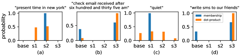
(a)

Figure 2: Distributions over slices (base, $s1$= Length, $s2$=Time and $s3$=Email) of random test samples that are from membership and dot-product attention mechanisms. In (a)(c) membership attention shows higher confidence while dot-product attention gives higher confidence in (b)(d). Top rows are the utterances from the test set.

4 Experiments

We performed our experiments on a binary classification task with linguistic acceptability and on a multi-class classification task with intent detection.

	F1			F1 Lift(%)		MCC			MCC Lift(%)
Methods	Overall	S1	S2	Avg.	Max.	Overall	S1	S2	Avg.	Max.
Baseline	0.70	0.60	0.65	—	—	0.24	0.18	0.22	—	—
SBL	0.69	0.71	0.72	9.0 %	11.0%	0.23	0.20	0.24	2.0%	2.0%
SBL-MoA $\oplus$	0.70	0.71	0.68	7.0%	11.0%	0.25	0.24	0.20	2.0%	6.0%
SBL-MoA $\otimes$	0.69	0.72	0.71	9.0%	12.0%	0.24	0.24	0.25	4.5%	6.0%
SBL-MoA-S $\oplus$	0.69	0.67	0.68	5.0%	7.0%	0.24	0.25	0.18	1.5%	7.0%
SBL-MoA-S $\otimes$	0.69	0.69	0.71	7.5%	9.0%	0.26	0.28	0.22	5.0%	10.0%
SBL-MoA-H $\oplus$	0.70	0.69	0.70	7.0%	9.0%	0.25	0.28	0.26	8.0%	10.0%
SBL-MoA-H $\otimes$	0.69	0.69	0.65	4.5%	9.0%	0.25	0.22	0.32	7.0%	10.0%

Table 2: The results on CoLA test datasets. F1-score and MCC are reported (averaged on 5 random runs for each model). $s1$=Long, and $s2$=Question.The lift is the averaged relative improvement across slices over baseline. The largest improvement is in bold and second largest lift number is in underline (same to Table 3).

4.1 Experimental Setup

Datasets and Metrics. The CoLA Warstadt et al. (2018) dataset has 8551 train and 527 development in domain samples. We randomly split it into train/val/test with 7200/878/1000 samples. As in Chen et al. (2019), we ensure the sample proportion in ground-truth are consistent across splits. We use F1-score and Matthews correlation coefficient (MCC) Matthews (1975) as our metrics. The NLU dataset Liu et al. (2019) for intent detection contains 25k user utterances across 64 intents. We randomly split it into train/val/test with ratio 0.7:0.1:0.2. We use the accuracy and F1-score as our metrics.

		Acc			Acc Lift(%)		F1				F1 Lift(%)
Methods	Overall	S1	S2	S3	Avg.	Max.	Overall	S1	S2	S3	Avg.	Max.
Baseline	0.7413	0.73	0.74	0.73	—	—	0.7404	0.74	0.72	0.74	—	—
SBL	0.7422	0.75	0.76	0.75	2.0%	2.0%	0.7418	0.74	0.72	0.75	0.3%	1.0%
SBL-MoA $\oplus$	0.7414	0.74	0.77	0.74	1.7%	3.0%	0.7390	0.74	0.73	0.74	0.3%	1.0%
SBL-MoA $\otimes$	0.7440	0.80	0.73	0.76	3.0%	7.0%	0.7411	0.77	0.74	0.74	1.7%	3.0%
SBL-MoA-S $\oplus$	0.7403	0.74	0.75	0.73	0.7%	1.0%	0.7403	0.73	0.73	0.76	0.7%	2.0%
SBL-MoA-S $\otimes$	0.7424	0.75	0.72	0.75	0.7%	2.0%	0.7421	0.75	0.74	0.74	1.0%	2.0%
SBL-MoA-H $\oplus$	0.7405	0.73	0.74	0.73	0.0%	0.0%	0.7397	0.76	0.74	0.76	2.0%	2.0%
SBL-MoA-H $\otimes$	0.7418	0.74	0.73	0.75	0.7%	2.0%	0.7401	0.75	0.74	0.74	1.0%	2.0%

Table 3: The results on intent detection. Accuracy and F1 scores are reported. $s1$=Length, $s2$=Time, $s3$=Email are the slices that we monitor and aim to improve. The experts’ confidence scores are not used as discussed in Sec.3.

Compared Methods. We implemented and compared the following methods:

• Baseline: A three-layer feed-forward network.

• SBL: Slice-based learning Chen et al. (2019).

• SBL-MoA: Our approach that extends SBL with a mixture of attentions (MoA).

For SBL-MoA, we developed multiple variants with Gumbel-Softmax. SBL-MoA-S (SBL-MoA-H) are the variant models with soft (hard) sampling from a Gumbel-Softmax distributions. We also tested the way that membership attention and dot-product interact with each other with $\oplus$ (element-wise addition) and $\otimes$ (element-wise multiplication).

Implementation Details. BERT-base Devlin et al. (2019) in sentence-transformer Thakur et al. (2020) is used as the backbone model. We use 128 hidden units for all models, which are implemented with Pytorch Paszke et al. (2019). A dropout (p=0.5) is applied after input layer. The models are trained with Adam (0.001) Kingma and Ba (2014), with weight decay of 0.01 and 0.001 for the two tasks, respectively. All models are trained with a maximum of 500 epochs with early stopping (patience=50). The best models are selected based on model performance on the validation sets. The temperature $\tau=1.0$ is fixed in all the experiments.

4.2 Results on Linguistic Acceptability

Table 2 presents the results on CoLA. First, slice-based models (i.e., SBL, SBL-MoA, and its variants) show that they can maintain (or improve) the original overall performance. Second, we observe that they achieve obvious performance lift on the monitored slices. For instance, SBL achieves an average 9% F1 score over the baseline. The proposed method (SBL-MoA, $\otimes$) achieves an average of 9% and maximum 12% lift. For MCC, the best performer is SBL-MoA-H, which achieves an average $\geqslant$7% and maximum 10% as compared to the baseline. It outperforms SBL by $\geqslant$ 5%. Also, we notice that using operator $\otimes$ (element-wise multiplication) between the attention mechanisms lead to better performance as compared to $\oplus$.

4.3 Results on Intent Detection

Table 3 demonstrates that both SBL and SBL-MoA improve model performance on the monitored slices, with a similar (slightly better) overall performance on the base task. SBL-MoA variants achieve the best scores and outperform SBL by average 1% accuracy and 1.7% F1.

Figure 2 illustrates the slice distributions given some random samples. We denote $\mathbf{p}_{1}$ and $\mathbf{p}_{2}$ for membership and dot-product attention respectively. The experiments show that $\mathbf{p}_{1}$ and $\mathbf{p}_{2}$ reach an agreement on predicting the correct slices. Interestingly, the sample in (d) — “write sms to our friends”, in principle, should be sliced as “base”, but both attentions exhibit high confidence to $s3$=“Email”. We conjecture the reason is that all utterances are encoded with BERT which captures the similarity between the sample and the utterances in the “Email” slice.

5 Related Work

SBL Chen et al. (2019) is a novel programming model for critical data slices. It is an instance of weakly supervised learning Zhou (2018); Medlock and Briscoe (2007). The weak supervision data are generated from pre-defined labeling functions Ratner et al. (2016). SBL has shown better predictive performance compared to the mixture of experts Jacobs et al. (1991) and multi-task learning Caruana (1997), with reduced run-time cost and parameters Chen et al. (2019). The concept of SBL has been recently used in many applications. Penha et al. Penha and Hauff (2020) proposed to adapt SBL to improve ranking performance and capture the failures of the ranker model. Wang et al. Wang et al. (2021) recently implemented SBL in a commercial conversational AI system in order to handle the long-tail problem of imbalanced distribution in customer queries and further improved the performance of the conversational skill routing components Li et al. (2021); Kim et al. (2018b, a).

Our proposed mixture of attention (MoA) is an instance of multi-head attention Vaswani et al. (2017) but with different attention types. MoA can also be extended to include other attention types. We have shown the effectiveness of this mechanism in determining the slice distributions.

6 Conclusion

This paper extends SBL with MoA (SBL-MoA) to improve model performance on particular data slices. We empirically show that SBL-MoA yields better slice level performance lift to baseline and vanilla SBL with two NLU tasks: linguistic acceptability and intent detection.

References

- Caruana (1997) Rich Caruana. 1997. Multitask learning. Machine learning, 28(1):41–75.
- Chen et al. (2019) Vincent Chen, Sen Wu, Alexander J Ratner, Jen Weng, and Christopher Ré. 2019. Slice-based learning: A programming model for residual learning in critical data slices. In Advances in neural information processing systems, pages 9397–9407.
- Devlin et al. (2019) Jacob Devlin, Ming-Wei Chang, Kenton Lee, and Kristina Toutanova. 2019. Bert: Pre-training of deep bidirectional transformers for language understanding. In NAACL-HLT.
- Gumbel (1954) Emil Julius Gumbel. 1954. Statistical Theory of Extreme Values and Some Practical Applications. A Series of Lectures. Number 33. US Govt. Print. Office.
- Jacobs et al. (1991) Robert A Jacobs, Michael I Jordan, Steven J Nowlan, and Geoffrey E Hinton. 1991. Adaptive mixtures of local experts. Neural computation, 3(1):79–87.
- Jang et al. (2017) Eric Jang, Shixiang Gu, and Ben Poole. 2017. Categorical reparameterization with gumbel-softmax. ICLR.
- Kim et al. (2019) Najoung Kim, Roma Patel, Adam Poliak, Alex Wang, Patrick Xia, R Thomas McCoy, Ian Tenney, Alexis Ross, Tal Linzen, Benjamin Van Durme, et al. 2019. Probing what different nlp tasks teach machines about function word comprehension. NAACL HLT 2019, page 235.
- Kim et al. (2018a) Young-Bum Kim, Dongchan Kim, Joo-Kyung Kim, and Ruhi Sarikaya. 2018a. A scalable neural shortlisting-reranking approach for large-scale domain classification in natural language understanding. arXiv preprint arXiv:1804.08064.
- Kim et al. (2018b) Young-Bum Kim, Dongchan Kim, Anjishnu Kumar, and Ruhi Sarikaya. 2018b. Efficient large-scale neural domain classification with personalized attention. In Proceedings of the 56th Annual Meeting of the Association for Computational Linguistics (Volume 1: Long Papers), pages 2214–2224.
- Kingma and Ba (2014) Diederik P Kingma and Jimmy Ba. 2014. Adam: A method for stochastic optimization. arXiv preprint arXiv:1412.6980.
- Li et al. (2021) Han Li, Sunghyun Park, Aswarth Dara, Jinseok Nam, Sungjin Lee, Young-Bum Kim, Spyros Matsoukas, and Ruhi Sarikaya. 2021. Neural model robustness for skill routing in large-scale conversational ai systems: A design choice exploration. arXiv preprint arXiv:2103.03373.
- Li et al. (2018) Jian Li, Zhaopeng Tu, Baosong Yang, Michael R Lyu, and Tong Zhang. 2018. Multi-head attention with disagreement regularization. In Proceedings of the 2018 Conference on Empirical Methods in Natural Language Processing, pages 2897–2903.
- Liu et al. (2019) Xingkun Liu, Arash Eshghi, Pawel Swietojanski, and Verena Rieser. 2019. Benchmarking natural language understanding services for building conversational agents. In 10th International Workshop on Spoken Dialogue Systems Technology 2019.
- Maddison et al. (2017) Chris J. Maddison, Andriy Mnih, and Yee Whye Teh. 2017. The Concrete Distribution: A Continuous Relaxation of Discrete Random Variables. In 5th International Conference on Learning Representations (ICLR).
- Matthews (1975) Brian W Matthews. 1975. Comparison of the predicted and observed secondary structure of t4 phage lysozyme. Biochimica et Biophysica Acta (BBA)-Protein Structure, 405(2):442–451.
- Medlock and Briscoe (2007) Ben Medlock and Ted Briscoe. 2007. Weakly supervised learning for hedge classification in scientific literature. In Proceedings of the 45th annual meeting of the association of computational linguistics, pages 992–999.
- Paszke et al. (2019) Adam Paszke, Sam Gross, Francisco Massa, Adam Lerer, James Bradbury, Gregory Chanan, Trevor Killeen, Zeming Lin, Natalia Gimelshein, Luca Antiga, Alban Desmaison, Andreas Kopf, Edward Yang, Zachary DeVito, Martin Raison, Alykhan Tejani, Sasank Chilamkurthy, Benoit Steiner, Lu Fang, Junjie Bai, and Soumith Chintala. 2019. Pytorch: An imperative style, high-performance deep learning library. In H. Wallach, H. Larochelle, A. Beygelzimer, F. d'Alché-Buc, E. Fox, and R. Garnett, editors, Advances in Neural Information Processing Systems 32, pages 8024–8035.
- Penha and Hauff (2020) Gustavo Penha and Claudia Hauff. 2020. Slice-aware neural ranking. In Proceedings of the 5th International Workshop on Search-Oriented Conversational AI (SCAI), pages 1–6.
- Ratner et al. (2016) Alexander J Ratner, Christopher M De Sa, Sen Wu, Daniel Selsam, and Christopher Ré. 2016. Data programming: Creating large training sets, quickly. Advances in neural information processing systems, 29:3567–3575.
- Roy et al. (2020) Aurko Roy, Mohammad Saffar, Ashish Vaswani, and David Grangier. 2020. Efficient content-based sparse attention with routing transformers. arXiv preprint arXiv:2003.05997.
- Rumelhart et al. (1986) David E Rumelhart, Geoffrey E Hinton, and Ronald J Williams. 1986. Learning representations by back-propagating errors. nature, 323(6088):533–536.
- Thakur et al. (2020) Nandan Thakur, Nils Reimers, Johannes Daxenberger, and Iryna Gurevych. 2020. Augmented sbert: Data augmentation method for improving bi-encoders for pairwise sentence scoring tasks. arXiv preprint arXiv:2010.08240.
- Vaswani et al. (2017) Ashish Vaswani, Noam Shazeer, Niki Parmar, Jakob Uszkoreit, Llion Jones, Aidan N Gomez, Łukasz Kaiser, and Illia Polosukhin. 2017. Attention is all you need. In Advances in neural information processing systems, pages 5998–6008.
- Wang et al. (2021) Cheng Wang, Sun Kim, Taiwoo Park, Sajal Choudhary, Sunghyun Park, Young-Bum Kim, Ruhi Sarikaya, and Sungjin Lee. 2021. Handling long-tail queries with slice-aware conversational systems. arXiv preprint arXiv:2104.13216.
- Wang and Niepert (2019) Cheng Wang and Mathias Niepert. 2019. State-regularized recurrent neural networks. In International Conference on Machine Learning, pages 6596–6606.
- Warstadt et al. (2018) Alex Warstadt, Amanpreet Singh, and Samuel R Bowman. 2018. Neural network acceptability judgments. arXiv preprint arXiv:1805.12471.
- Zhou (2018) Zhi-Hua Zhou. 2018. A brief introduction to weakly supervised learning. National science review, 5(1):44–53.