PCA Initialization for Approximate Message Passing in Rotationally Invariant Models

Abstract

We study the problem of estimating a rank-$1$ signal in the presence of rotationally invariant noise—a class of perturbations more general than Gaussian noise. Principal Component Analysis (PCA) provides a natural estimator, and sharp results on its performance have been obtained in the high-dimensional regime. Recently, an Approximate Message Passing (AMP) algorithm has been proposed as an alternative estimator with the potential to improve the accuracy of PCA. However, the existing analysis of AMP requires an initialization that is both correlated with the signal and independent of the noise, which is often unrealistic in practice. In this work, we combine the two methods, and propose to initialize AMP with PCA. Our main result is a rigorous asymptotic characterization of the performance of this estimator. Both the AMP algorithm and its analysis differ from those previously derived in the Gaussian setting: at every iteration, our AMP algorithm requires a specific term to account for PCA initialization, while in the Gaussian case, PCA initialization affects only the first iteration of AMP. The proof is based on a two-phase artificial AMP that first approximates the PCA estimator and then mimics the true AMP. Our numerical simulations show an excellent agreement between AMP results and theoretical predictions, and suggest an interesting open direction on achieving Bayes-optimal performance.

1 Introduction

We consider the problem of estimating a rank-$1$ signal from a noisy data matrix. In the square symmetric case, the data matrix is modeled as

$${\boldsymbol{X}}=\frac{\alpha}{n}{\boldsymbol{u}}^{*}{{\boldsymbol{u}}^{*}}^{{\sf T}}+{\boldsymbol{W}}\in\mathbb{R}^{n\times n},$$ (1.1)

where ${\boldsymbol{u}}^{*}\in\mathbb{R}^{n}$ is the unknown rank-$1$ signal, ${\boldsymbol{W}}\in\mathbb{R}^{n\times n}$ is a symmetric noise matrix, and $\alpha>0$ captures the signal-to-noise ratio (SNR). In the rectangular case, we observe the data matrix

$${\boldsymbol{X}}=\frac{\alpha}{m}{\boldsymbol{u}}^{*}{{\boldsymbol{v}}^{*}}^{\sf T}+{\boldsymbol{W}}\in\mathbb{R}^{m\times n},$$ (1.2)

where ${\boldsymbol{u}}^{*}\in\mathbb{R}^{m}$ and ${\boldsymbol{v}}^{*}\in\mathbb{R}^{n}$ are the unknown signals, and ${\boldsymbol{W}}\in\mathbb{R}^{m\times n}$ is a rectangular noise matrix. A natural estimator of the signal in the symmetric case is the principal eigenvector of ${\boldsymbol{X}}$ (singular vectors, in the rectangular case). The performance of this principal component analysis (PCA) estimator and, more generally, the behavior of eigenvalues and eigenvectors of models like (1.1)-(1.2) has been widely studied in statistics [Joh01, Pau07] and random matrix theory [BBAP05, BS06, BGN11, BGN12, CDMF09, FP07, KY13].

If ${\boldsymbol{u}}^{*},{\boldsymbol{v}}^{*}$ are unstructured (e.g., they are uniformly distributed on a sphere), then it is not generally possible to improve on the PCA estimator. However, in a broad range of applications, the unknown signals have some underlying structure, e.g., they may be sparse, their entries may belong to a certain set, or they may be modelled using a prior distribution. Examples of structured matrix estimation problems include sparse PCA [DM14, JL09, ZHT06], non-negative PCA [LS99, MR16], community detection under the stochastic block model [Abb17, DAM16, Moo17], and group synchronization [PWBM18]. Since PCA is ill-equipped to capture the structure of the signal, we aim to improve on it using a family of iterative algorithms known as approximate message passing (AMP). AMP algorithms have two particularly attractive features: (i) they can be tailored to take advantage of prior information on the structure of the signal; and (ii) under suitable model assumptions, their performance in the high-dimensional limit is precisely characterized by a succinct deterministic recursion called state evolution [BM11, Bol14, JM13]. AMP algorithms have been applied to a wide range of inference problems: estimation in linear models [BM12, BM11, DMM09, KMS⁺12, MAYB13], generalized linear models [BKM⁺19, MXM19, MLKZ20, MV21a, Ran11, SR14, SC19], and low-rank matrix estimation with Gaussian noise [BMR20, DM14, FR18, KKM⁺16, LKZ17, MV21b]. The survey [FVRS21] provides a unified description of AMP for these applications. Using the state evolution analysis, it has been proved that AMP achieves Bayes-optimal performance in some Gaussian models [DM14, DJM13, MV21b], and a bold conjecture from statistical physics posits that AMP is optimal among polynomial-time algorithms.

We study rank-1 matrix estimation in the setting where the noise matrix ${\boldsymbol{W}}$ is rotationally invariant. This is a much milder assumption than ${\boldsymbol{W}}$ being Gaussian: it only imposes that the orthogonal matrices in the spectral decomposition of ${\boldsymbol{W}}$ are uniformly random, and allows for arbitrary eigenvalues/singular values. Hence, ${\boldsymbol{W}}$ can capture a more complex correlation structure, which is typical in applications. For the models (1.1)-(1.2) with rotationally invariant noise, AMP algorithms were derived in [ÇO19, OCW16] and generalized in [Fan20]. In particular, the AMP algorithm of [Fan20] for the problem (1.1) produces estimates ${\boldsymbol{u}}^{t}\in\mathbb{R}^{n}$ as follows:

$${\boldsymbol{u}}^{t}={\sf u}_{t}({\boldsymbol{f}}^{t-1}),\quad{\boldsymbol{f}}^{t}={\boldsymbol{X}}{\boldsymbol{u}}^{t}-\sum_{i=1}^{t}{\sf b}_{t,i}{\boldsymbol{u}}^{i},\qquad t\geq 2.$$ (1.3)

The iteration is initialized with a pilot estimate ${\boldsymbol{u}}^{1}$. We can interpret (1.3) as a generalized power method. Recall that the power method approximates the principal eigenvector of ${\boldsymbol{X}}$ using the iterative updates $\bar{{\boldsymbol{u}}}^{t}={\boldsymbol{X}}\bar{{\boldsymbol{u}}}^{t-1}/\|{\boldsymbol{X}}\bar{{\boldsymbol{u}}}^{t-1}\|$. For each $t$, the function ${\sf u}_{t}$ can be chosen to exploit any structural information known about the signal (e.g., sparsity). The “memory” coefficients $\{{\sf b}_{t,1},\ldots,{\sf b}_{t,t}\}$ have a specific form to ensure that the iterates $({\boldsymbol{f}}^{t},{\boldsymbol{u}}^{t+1})$ have desirable statistical properties captured by state evolution. A rigorous state evolution result for the iteration (1.3) is established in [Fan20], but the algorithm and its analysis require an initialization ${\boldsymbol{u}}^{1}$ that is correlated with the unknown signal and independent of the noise ${\boldsymbol{W}}$. In practice, one typically does not have access to such an initialization.

Main contribution.

In this paper, we propose an AMP algorithm initialized via the PCA estimator, namely, the principal eigenvector of ${\boldsymbol{X}}$ for the square case (1.1) and the left singular vector of ${\boldsymbol{X}}$ for the rectangular case (1.2). Our main technical contribution is a state evolution result for this AMP algorithm, which gives a rigorous characterization of its performance in the high-dimensional limit. The challenge is that, as the PCA initialization depends on the noise matrix ${\boldsymbol{W}}$, one cannot apply the state evolution machinery of [Fan20]. To circumvent this issue, our key idea is to construct and analyze a two-phase artificial AMP algorithm. In the first phase, the artificial AMP performs a power method approaching the PCA estimator; and in the second phase, it mimics the behavior of the true AMP. We remark that the artificial AMP only serves as a proof technique. Thus, we can initialize it with a vector correlated with the signal ${\boldsymbol{u}}^{*}$ and independent of the noise matrix ${\boldsymbol{W}}$, which allows us to analyze it using the existing state evolution result.

Our analysis is tight in the sense that our AMP algorithm can be initialized with PCA whenever the PCA estimate has strictly positive correlation with the signal. This requires showing that, when PCA is effective, the state evolution of the first phase of the artificial AMP has a unique fixed point. To obtain such a result, we exploit free probability tools developed in [BGN11, BGN12]. The agreement between the practical performance of AMP and the theoretical predictions of state evolution is demonstrated via numerical results for different spectral distributions of ${\boldsymbol{W}}$. Our simulations also show that the performance of AMP—as well as its ability to improve upon the PCA initialization—crucially depends on the choice of the denoising functions ${\sf u}_{t}$ in the algorithm. Thus, the design of a Bayes-optimal AMP remains an exciting avenue for future research.

Related work.

The asymptotic Bayes-optimal error for low-rank matrix estimation has been precisely characterized for Gaussian noise [BDM⁺16, LM19], but remains an open problem for rotationally invariant noise. An AMP algorithm with PCA initialization was proposed in [MV21b] for the Gaussian setting, and it was shown to be Bayes-optimal for some signal priors. A recent paper by Zhong et al. [ZSF21b] shows how AMP with PCA initialization can be used for estimating the top-$k$ principal components in applications such as high-dimensional genomics datasets. The authors use an empirical Bayes method to determine a joint prior distribution for the $k$ principal components, and assuming a Gaussian noise model, employ an AMP algorithm tailored to the prior to improve the PCA estimates of the principal components.

Both our AMP algorithm and proof technique differ significantly from those for Gaussian noise. When ${\boldsymbol{W}}$ is Gaussian, the PCA initialization affects only the first iteration of AMP. In contrast, for more general noise distributions, the AMP algorithm and its associated state evolution require a correction term at every iteration to account for the PCA initialization. This is due to the fact that, while AMP has a single memory term in the Gaussian case, more general noise distributions lead to a more involved memory structure, as in (1.3). As regards the proof technique, the argument of [MV21b] consists of decoupling the PCA estimate from the bulk of the spectrum of ${\boldsymbol{X}}$. In contrast, our approach is based on a two-phase artificial AMP algorithm. This technique has proved successful in the context of generalized linear models [MTV20, MV21a], albeit for Gaussian measurements. Other extensions of AMP beyond the Gaussian setting include Orthogonal AMP [MP17, Tak20], Vector AMP [GAK20a, GAK20b, RSF19, SRF16], convolutional AMP [Tak21] and Memory AMP [LHK20]. These algorithms have been derived specifically for linear or generalized linear models, and extending them (with a practical initialization method) to low-rank matrix estimation is an interesting research direction.

Finally, we mention the recent independent work of Zhong et al. [ZSF21a], which appeared after the original submission of our paper. This work generalizes AMP with PCA initialization to the problem of estimating rank-$k$ matrices in rotationally invariant noise, for $k\geq 1$. We remark that, in order to prove a state evolution result for AMP initialized with PCA, in [ZSF21a] it is assumed that the signal strength is sufficiently large. In contrast, our result holds for any signal strength such that the PCA method is effective, but we require the free cumulants of the noise matrix to be non-negative. We also note that, when the signal strength is large, the assumption on the free cumulants can be automatically satisfied (see the footnote on p.1).

2 Preliminaries

Notation and definitions.

Given $a\in\mathbb{R}$, we define $(a)_{+}=\max(a,0)$. Given two integers $i\leq j$, we define $[i,j]=\{i,\ldots,j\}$. If $i>j$, then $[i,j]$ denotes the empty set; products over the empty set are taken to be 1. Given a vector ${\boldsymbol{x}}\in\mathbb{R}^{n}$, we denote by $\|{\boldsymbol{x}}\|$ its Euclidean norm and by $\langle{\boldsymbol{x}}\rangle$ its empirical mean, i.e., $\langle{\boldsymbol{x}}\rangle=\frac{1}{n}\sum_{i=1}^{n}x_{i}$. The empirical distribution of ${\boldsymbol{x}}=(x_{1},\ldots,x_{n})^{\sf T}$ is given by $\frac{1}{n}\sum_{i=1}^{n}\delta_{x_{i}}$, where $\delta_{x_{i}}$ denotes a Dirac delta mass on $x_{i}$. The notation ${\boldsymbol{x}}\stackrel{{\scriptstyle\mathclap{W}}}{{\longrightarrow}}X$ denotes convergence of the empirical distribution of ${\boldsymbol{x}}$ to the random variable $X$ in Wasserstein distance at all orders. Given a symmetric square matrix ${\boldsymbol{A}}\in\mathbb{R}^{n\times n}$, we denote by $\lambda_{1}({\boldsymbol{A}})\geq\lambda_{2}({\boldsymbol{A}})\geq\ldots\geq\lambda_{n}({\boldsymbol{A}})$ its eigenvalues sorted in decreasing order. Given a rectangular matrix ${\boldsymbol{A}}\in\mathbb{R}^{m\times n}$, with $m<n$, we denote by $\sigma_{1}({\boldsymbol{A}})\geq\sigma_{2}({\boldsymbol{A}})\geq\ldots\sigma_{m}({\boldsymbol{A}})$ its singular values sorted in decreasing order.

Rank-$1$ estimation – Symmetric square matrices.

Consider the problem of estimating the signal ${\boldsymbol{u}}^{*}\in\mathbb{R}^{n}$ from the data matrix ${\boldsymbol{X}}$ in (1.1). We assume that ${\boldsymbol{W}}$ is rotationally invariant in law, i.e., ${\boldsymbol{W}}={\boldsymbol{O}}^{\sf T}{\boldsymbol{\Lambda}}{\boldsymbol{O}}$, where ${\boldsymbol{\Lambda}}={\rm diag}({\boldsymbol{\lambda}})$ is a diagonal matrix containing the eigenvalues of ${\boldsymbol{W}}$ and ${\boldsymbol{O}}$ is a Haar orthogonal matrix independent of ${\boldsymbol{\Lambda}}$. As $n\to\infty$, we assume that the empirical distributions of ${\boldsymbol{\lambda}}$ and ${\boldsymbol{u}}^{*}$ satisfy

$${\boldsymbol{\lambda}}\stackrel{{\scriptstyle\mathclap{W}}}{{\longrightarrow}}\Lambda\quad\text{ and }\quad{\boldsymbol{u}}^{*}\stackrel{{\scriptstyle\mathclap{W}}}{{\longrightarrow}}U_{*},$$ (2.1)

where $\Lambda$ and $U_{*}$ represent the limiting spectral distribution of the noise and the prior on the signal, respectively. We take $\|{\boldsymbol{u}}\|=\sqrt{n}$ so that $\mathbb{E}\{U_{*}^{2}\}=\lim_{n\to\infty}\frac{1}{n}\|{\boldsymbol{u}}^{*}\|^{2}=1$. We assume that the moment ${\mathbb{E}}\{U_{*}^{2+\varepsilon}\}<\infty$ for some $\varepsilon>0$. We also assume that $\Lambda$ has compact support, and denote by $b$ the supremum of this support. We denote by $\{\kappa_{k}\}_{k\geq 1}$ the free cumulants corresponding to the moments $\{m_{k}\}_{k\geq 1}$ of the empirical eigenvalue distribution of ${\boldsymbol{X}}$ excluding its largest eigenvalue, i.e., $m_{k}=\frac{1}{n}\sum_{i=2}^{n}\lambda_{i}({\boldsymbol{X}})^{k}$ (for details, see (A.1)-(A.2) in Appendix A). The assumption (2.1) implies that, as $n\to\infty$, $m_{k}\to m^{\infty}_{k}=\mathbb{E}\{\Lambda^{k}\}$ and $\kappa_{k}\to\kappa^{\infty}_{k}$, where $\{m_{k}^{\infty}\}_{k\geq 1}$ and $\{\kappa_{k}^{\infty}\}_{k\geq 1}$ are respectively moments and free cumulants of $\Lambda$.

PCA – Symmetric square matrices.

Let ${\boldsymbol{u}}_{\rm PCA}$ be the principal eigenvector of ${\boldsymbol{X}}$, and define $\alpha_{\rm s}=1/G(b^{+})$, where $G(z)=\mathbb{E}\{(z-\Lambda)^{-1}\}$ is the Cauchy transform of $\Lambda$, and $G(b^{+})=\lim_{z\to b^{+}}G(z)$. Then, for $\alpha>\alpha_{\rm s}$, $\lambda_{1}({\boldsymbol{X}})\stackrel{{\scriptstyle\mathclap{\mbox{\footnotesize a.s.}}}}{{\longrightarrow}}G^{-1}(1/\alpha)$ and $\lambda_{2}({\boldsymbol{X}})\stackrel{{\scriptstyle\mathclap{\mbox{\footnotesize a.s.}}}}{{\longrightarrow}}b$, where $G^{-1}$ is the inverse of $G$; see Theorem 2.1 in [BGN11]. Furthermore, Theorem 2.2 in [BGN11] gives that, for $\alpha>\alpha_{\rm s}$,

$$\frac{\langle{\boldsymbol{u}}_{\rm PCA},{\boldsymbol{u}}^{*}\rangle^{2}}{n}\stackrel{{\scriptstyle\mathclap{\mbox{\footnotesize a.s.}}}}{{\longrightarrow}}\rho_{\alpha}^{2}=\frac{-1}{\alpha^{2}G^{\prime}(G^{-1}(1/\alpha))}>0.$$ (2.2)

In words, above the spectral threshold $\alpha_{\rm s}$, the principal eigenvalue of ${\boldsymbol{X}}$ escapes the bulk of the spectrum and its associated eigenvector becomes strictly correlated with the signal ${\boldsymbol{u}}^{*}$.

Rank-$1$ estimation – Rectangular matrices.

Consider now the problem of estimating the signals ${\boldsymbol{u}}^{*}\in\mathbb{R}^{m}$ and ${\boldsymbol{v}}^{*}\in\mathbb{R}^{n}$ given the rectangular data matrix ${\boldsymbol{X}}$ in (1.2). Without loss of generality, we assume that $m\leq n$ (if $m>n$, one can just exchange the role of ${\boldsymbol{u}}^{*}$ and ${\boldsymbol{v}}^{*}$ and consider ${\boldsymbol{X}}^{\sf T}$ in place of ${\boldsymbol{X}}$). We assume that $W$ is bi-rotationally invariant in law, i.e., ${\boldsymbol{W}}={\boldsymbol{O}}^{\sf T}{\boldsymbol{\Lambda}}{\boldsymbol{Q}}$, where ${\boldsymbol{\Lambda}}={\rm diag}({\boldsymbol{\lambda}})$ is a $m\times n$ diagonal matrix containing the singular values of ${\boldsymbol{W}}$, and ${\boldsymbol{O}}$, ${\boldsymbol{Q}}$ are Haar orthogonal matrices independent of one another and also of ${\boldsymbol{\Lambda}}$. As $n\to\infty$, we assume that ${\boldsymbol{\lambda}}\stackrel{{\scriptstyle\mathclap{W}}}{{\longrightarrow}}\Lambda$, ${\boldsymbol{u}}^{*}\stackrel{{\scriptstyle\mathclap{W}}}{{\longrightarrow}}U_{*}$, ${\boldsymbol{v}}^{*}\stackrel{{\scriptstyle\mathclap{W}}}{{\longrightarrow}}V_{*}$ and $m/n\to\gamma$, for some constant $\gamma\in(0,1]$. We take $\|{\boldsymbol{u}}\|=\sqrt{m}$ and $\|{\boldsymbol{v}}\|=\sqrt{n}$ so that $\mathbb{E}\{U_{*}^{2}\}=\mathbb{E}\{V_{*}^{2}\}=1$. As before, $b<\infty$ is the supremum of the compact support of $\Lambda$, and $U_{*},V_{*}$ are assumed to have finite $(2+\varepsilon)$-th moment for some $\varepsilon>0$ . To analyze PCA using the framework in [BGN12], we also assume that the entries of ${\boldsymbol{u}}^{*}$ and ${\boldsymbol{v}}^{*}$ are i.i.d., and their law has zero mean and satisfies a log-Sobolev inequality. We denote by $\{\kappa_{2k}\}_{k\geq 1}$ the rectangular free cumulants associated to the even moments $\{m_{2k}\}_{k\geq 1}$, with $m_{2k}=\frac{1}{m}\sum_{i=2}^{m}\sigma_{i}({\boldsymbol{X}})^{2k}$ (for details, see (A.11)-(A.12) in Appendix A). Furthermore, as $n,m\to\infty$, $m_{2k}\to m^{\infty}_{2k}=\mathbb{E}\{\Lambda^{2k}\}$ and $\kappa_{2k}\to\kappa_{2k}^{\infty}$, where $\{m_{2k}^{\infty}\}_{k\geq 1}$ and $\{\kappa_{2k}^{\infty}\}_{k\geq 1}$ are respectively even moments and rectangular free cumulants of $\Lambda$.

PCA – Rectangular matrices.

Denote by ${\boldsymbol{u}}_{\rm PCA}$ and ${\boldsymbol{v}}_{\rm PCA}$ the left and right principal singular vectors of ${\boldsymbol{X}}$, and define $\tilde{\alpha}_{\rm s}=1/\sqrt{D(b^{+})}$, where $D(z)=\phi(z)\bar{\phi}(z)$, $\phi(z)=\mathbb{E}\{z/(z^{2}-\Lambda^{2})\}$, $\bar{\phi}(z)=\gamma\phi(z)+(1-\gamma)/z$, and $D(b^{+})=\lim_{z\to b^{+}}D(z)$. Note that the singular value of the rank-one signal $\frac{\alpha}{m}{\boldsymbol{u}}^{*}{{\boldsymbol{v}}^{*}}^{\sf T}$ is $\tilde{\alpha}\triangleq\alpha/\sqrt{\gamma}$. Then, for $\tilde{\alpha}>\tilde{\alpha}_{\rm s}$, $\sigma_{1}({\boldsymbol{X}})\stackrel{{\scriptstyle\mathclap{\mbox{\footnotesize a.s.}}}}{{\longrightarrow}}D^{-1}(1/\tilde{\alpha}^{2})$ and $\sigma_{2}({\boldsymbol{X}})\stackrel{{\scriptstyle\mathclap{\mbox{\footnotesize a.s.}}}}{{\longrightarrow}}b$; see Theorem 2.8 in [BGN12]. Furthermore, Theorem 2.9 in [BGN12] gives that, for $\tilde{\alpha}>\tilde{\alpha}_{\rm s}$,

$$\frac{\langle{\boldsymbol{u}}_{\rm PCA},{\boldsymbol{u}}^{*}\rangle^{2}}{m}\stackrel{{\scriptstyle\mathclap{\mbox{\footnotesize a.s.}}}}{{\longrightarrow}}\Delta_{{\rm PCA}}=\frac{-2\phi(D^{-1}(1/\tilde{\alpha}^{2}))}{\tilde{\alpha}^{2}D^{\prime}(D^{-1}(1/\tilde{\alpha}^{2}))}>0,$$ (2.3)

$$\frac{\langle{\boldsymbol{v}}_{\rm PCA},{\boldsymbol{v}}^{*}\rangle^{2}}{n}\stackrel{{\scriptstyle\mathclap{\mbox{\footnotesize a.s.}}}}{{\longrightarrow}}\Gamma_{{\rm PCA}}=\frac{-2\bar{\phi}(D^{-1}(1/\tilde{\alpha}^{2}))}{\tilde{\alpha}^{2}D^{\prime}(D^{-1}(1/\tilde{\alpha}^{2}))}>0.$$ (2.4)

In words, above the spectral threshold $\tilde{\alpha}_{\rm s}$, the principal singular value escapes from the bulk of the spectrum and the left/right principal singular vectors become correlated with the signal ${\boldsymbol{u}}^{*}$/${\boldsymbol{v}}^{*}$.

3 PCA Initialization for Approximate Message Passing

3.1 Symmetric Square Matrices

We consider a family of Approximate Message Passing (AMP) algorithms to estimate ${\boldsymbol{u}}^{*}$ from ${\boldsymbol{X}}=\frac{\alpha}{n}{\boldsymbol{u}}^{*}{{\boldsymbol{u}}^{*}}^{{\sf T}}+{\boldsymbol{W}}$. We initialize using the PCA estimate ${\boldsymbol{u}}_{\rm PCA}$:

$${\boldsymbol{u}}^{1}=\sqrt{n}{\boldsymbol{u}}_{\rm PCA},\quad{\boldsymbol{f}}^{1}={\boldsymbol{X}}{\boldsymbol{u}}^{1}-{\sf b}_{1,1}{\boldsymbol{u}}^{1},$$ (3.1)

with ${\sf b}_{1,1}=\sum_{i=0}^{\infty}\kappa_{i+1}\alpha^{-i}$. Then, for $t\geq 2$, the algorithm computes

$${\boldsymbol{u}}^{t}={\sf u}_{t}({\boldsymbol{f}}^{t-1}),\quad{\boldsymbol{f}}^{t}={\boldsymbol{X}}{\boldsymbol{u}}^{t}-\sum_{i=1}^{t}{\sf b}_{t,i}{\boldsymbol{u}}^{i},$$ (3.2)

where the memory coefficients $\{{\sf b}_{t,i}\}_{i\in[1,t]}$ are given by ${\sf b}_{t,t}=\kappa_{1}$, and

$$\begin{split}&{\sf b}_{t,1}=\prod_{\ell=2}^{t}\langle{\sf u}_{\ell}^{\prime}({\boldsymbol{f}}^{\ell-1})\rangle\sum_{i=0}^{\infty}\kappa_{i+t}\alpha^{-i},\quad{\sf b}_{t,t-j}=\kappa_{j+1}\prod_{i=t-j+1}^{t}\langle{\sf u}_{i}^{\prime}({\boldsymbol{f}}^{i-1})\rangle,\ \mbox{ for }\,\,(t-j)\in[2,t-1].\end{split}$$ (3.3)

Here, the function ${\sf u}_{t}:\mathbb{R}\to\mathbb{R}$ is continuously differentiable and Lipschitz, it is applied component-wise to vectors, i.e., ${\sf u}_{t}({\boldsymbol{f}}^{t-1})=({\sf u}_{t}(f^{t-1}_{1}),\ldots,{\sf u}_{t}(f^{t-1}_{n}))$, and ${\sf u}_{t}^{\prime}$ denotes its derivative. The AMP algorithm in (3.1)-(3.3) is similar to the one in [Fan20, Sec. 3.1] (and the ones in [ÇO19, OCW16]), with the main differences being the initialization ${\boldsymbol{u}}^{1}$ and the formula for the memory term ${\sf b}_{t,1}$. We highlight that the algorithm does not require the knowledge of $\alpha$ or of the noise distribution. In fact, $\alpha$ can be consistently estimated from the principal eigenvalue of ${\boldsymbol{X}}$ via $\hat{\alpha}=(G(\lambda_{1}({\boldsymbol{X}})))^{-1}$. Furthermore, one can compute the moments $\{m_{k}\}_{k\geq 1}$ of the empirical eigenvalue distribution of ${\boldsymbol{X}}$ (excluding its largest one) and, from these, deduce the free cumulants $\{\kappa_{k}\}_{k\geq 1}$.

The asymptotic empirical distribution of the iterates ${\boldsymbol{u}}^{t},{\boldsymbol{f}}^{t}$, for $t\geq 1$, can be succinctly characterized via a deterministic recursion, called state evolution, and expressed via a sequence of mean vectors ${\boldsymbol{\mu}}_{K}=(\mu_{t})_{t\in[1,K]}$ and covariance matrices ${\boldsymbol{\Sigma}}_{K}=(\sigma_{s,t})_{s,t\in[1,K]}$. For $K=1$, set $\mu_{1}=\alpha\rho_{\alpha}$ and $\sigma_{11}=\alpha^{2}(1-\rho_{\alpha}^{2})$, with $\rho_{\alpha}$ given in (2.2). Then define ${\boldsymbol{\mu}}_{K+1},{\boldsymbol{\Sigma}}_{K+1}$ from ${\boldsymbol{\mu}}_{K},{\boldsymbol{\Sigma}}_{K}$ as follows. Let

$$(F_{1},\ldots,F_{K})={\boldsymbol{\mu}}_{K}U_{*}+(Z_{1},\ldots,Z_{K}),\text{ where }(Z_{1},\ldots,Z_{K})\sim\mathcal{N}(\boldsymbol{0},{\boldsymbol{\Sigma}}_{K}),\quad$$ (3.4)

$$U_{t}={\sf u}_{t}(F_{t-1})\ \text{ for }2\leq t\leq K+1,\quad\text{ and }\quad U_{t}=\frac{F_{1}}{\alpha}\ \text{ for }-\infty<t\leq 1.$$ (3.5)

Then, the entries of ${\boldsymbol{\mu}}_{K+1}$ are given by $\mu_{t}=\alpha{\mathbb{E}}\{U_{t}U_{*}\}$ for $t\in[1,K+1]$. Furthermore, the entries of ${\boldsymbol{\Sigma}}_{K+1}$ can be expressed via the following formula, for $s,t\in[1,K+1]$:

$$\sigma_{s,t} =\sum_{j=0}^{\infty}\sum_{k=0}^{\infty}\kappa_{j+k+2}^{\infty}\left(\frac{1}{\alpha}\right)^{(k-t+1)_{+}+(j-s+1)_{+}}\cdot\hskip 10.00002pt{\mathbb{E}}\{U_{s-j}U_{t-k}\}\cdot\Big{(}\prod_{i=\max(2,s+1-j)}^{s}{\mathbb{E}}\{{\sf u}_{i}^{\prime}(F_{i-1})\}\Big{)}\cdot\Big{(}\prod_{i=\max(2,t+1-k)}^{t}{\mathbb{E}}\{{\sf u}_{i}^{\prime}(F_{i-1})\}\Big{)}.$$ (3.6)

Our main result, Theorem 1, shows that for $t\geq 1$, the empirical joint distribution of the entries of $({\boldsymbol{u}}^{*},{\boldsymbol{f}}^{1},\ldots,{\boldsymbol{f}}^{t})$ converges in Wasserstein distance $W_{2}$ to the law of the random vector $(U_{*},F_{1},\ldots,F_{t})$. We provide a proof sketch in Section 5, and the complete proof is deferred to Appendix B. This result is stated in terms of pseudo-Lipschitz test functions. A function $\psi:\mathbb{R}^{m}\to\mathbb{R}$ is pseudo-Lipschitz of order $2$, i.e., $\psi\in{\rm PL}(2)$, if there is a constant $C>0$ such that

$$\left\lVert{\psi({\boldsymbol{x}})-\psi({\boldsymbol{y}})}\right\rVert\leq C(1+\|{\boldsymbol{x}}\|+\|{\boldsymbol{y}}\|)\left\lVert{{\boldsymbol{x}}-{\boldsymbol{y}}}\right\rVert.$$ (3.7)

The equivalence between convergence in terms of ${\rm PL}(2)$ functions and convergence in $W_{2}$ distance follows from [Vil08, Definition 6.7 and Theorem 6.8].

Theorem 1.

In the square symmetric model (1.1), assume that $\alpha>\alpha_{\rm s}$, and that the free cumulants of order 2 and higher are non-negative, i.e., $\kappa_{k}^{\infty}\geq 0$ for $k\geq 2$. Consider the AMP algorithm with PCA initialization in (3.1)-(3.2), with continuously differentiable and Lipschitz functions ${\sf u}_{t}:\mathbb{R}\to\mathbb{R}$. (Without loss of generality, assume that $\langle{\boldsymbol{u}}^{*},{\boldsymbol{u}}^{{\rm PCA}}\rangle\geq 0$.)

Then, for $t\geq 1$ and any PL($2$) function $\psi:\mathbb{R}^{2t+2}\to\mathbb{R}$, we almost surely have:

$$\lim_{n\to\infty}\frac{1}{n}\sum_{i=1}^{n}\psi(u^{*}_{i},u^{1}_{i},\ldots,u^{t+1}_{i},f^{1}_{i},\ldots f^{t}_{i})={\mathbb{E}}\left\{\psi(U_{*},U_{1},\ldots,U_{t+1},F_{1},\ldots,F_{t})\right\},$$ (3.8)

where $U_{1},\ldots,U_{t+1}$ and $F_{1},\ldots,F_{t}$ are defined in (3.4).

Assumptions of the theorem.

The basic assumption that the noise matrix is rotationally invariant is rather mild as it allows for arbitrary eigenvalue distributions. The assumption $\alpha>\alpha_{\rm s}$ ensures that the PCA initialization is correlated with the signal. This condition is necessary and sufficient for PCA to be effective: under the additional requirement that $G^{\prime}(b)=-\infty$, we have that, if $\alpha<\alpha_{\rm s}$, then the normalized correlation between ${\boldsymbol{u}}_{\rm PCA}$ and ${\boldsymbol{u}}^{*}$ vanishes almost surely; see Theorem 2.3 of [BGN11]. Conversely for $\alpha>\alpha_{\rm s}$, the asymptotic correlation is strictly non-zero and given by (2.2).

Non-negativity of free cumulants: The assumption that $\kappa^{\infty}_{k}\geq 0$ for $k\geq 2$ appears to be an artifact of the proof technique. As detailed in the proof sketch in Section 5, this assumption is needed to show that the state evolution of the artificial AMP in the first phase has a unique fixed point. We expect our approach to generalize to any limiting noise distribution $\Lambda$ with compact support, and defer such a generalization to future work. In support of this view, the simulations of Section 4 verify the claim of Theorem 1 in a setting where the free cumulants of $\Lambda$ have alternating signs (corresponding to an eigenvalue distribution $\Lambda\sim\text{Uniform}[-1/2,1/2]$; see Figs. 1b-1d and 2b–2d). Finally, we remark that, if ${\boldsymbol{W}}$ follows a Marcenko-Pastur distribution (${\boldsymbol{W}}={\boldsymbol{A}}{\boldsymbol{A}}^{\sf T}$, where ${\boldsymbol{A}}$ has i.i.d. Gaussian entries), then the free cumulants of $\Lambda$ are all equal and strictly positive; see [MS17, Chap. 2, Exercise 11]. Thus, the assumption of Theorem 1 holds for noise distributions that are sufficiently close to the Marcenko-Pastur one, or for sufficiently large values of the signal-to-noise ratio $\alpha$.

Continuous differentiability and other technical assumptions: The assumption that ${\sf u}_{t}$ is continuously differentiable can be weakened to: (i) ${\sf u}_{t}$ being differentiable almost everywhere, and (ii) satisfying a mild non-degeneracy condition (Assumption 4.2(e) in [Fan20]). In this way, we can cover most practically relevant choices of ${\sf u}_{t}$ such as soft thresholding and ReLU. Theorem 1 also requires the technical assumptions in (2.1) and the text below it: convergence of the empirical distributions of the signal and of the eigenvalues of the noise matrix; boundedness of the $(2+\varepsilon)$-moment of the signal; and compact support of the spectrum of the noise matrix. We regard these technical assumptions as minor, and remark that they are quite standard in the literature. For the rectangular case, we also need the additional assumption that the law of the signal is zero mean and satisfies a log-Sobolev inequality, which is necessary to apply the framework in [BGN11].

How PCA initialization influences AMP.

The form of the memory coefficient ${\sf b}_{t,1}$ in (3.3) reflects the PCA initialization of the AMP iteration. PCA initialization can be interpreted as the result of a first AMP phase with linear denoisers (see the proof sketch in Sec. 5). The coefficient ${\sf b}_{t,1}$ multiplying the initialization ${\boldsymbol{u}}_{1}$ represents the cumulative effect of this first AMP phase leading to the PCA estimate. The main differences from the AMP algorithm in [Fan20] (where the initialization is independent of ${\boldsymbol{W}}$) are the expressions for the coefficient ${\sf b}_{t,1}$ and the state evolution parameters $\sigma_{s,t}$ (compare (3.3) and (3.6) in this paper with (1.15) and (1.17) in [Fan20]). One can interpret the new form of ${\sf b}_{t,1}$ and $\sigma_{s,t}$ as a memory of the PCA initialization. For the special case of Gaussian noise, the spectral initialization only affects the first iteration of AMP [MV21b]. This is due to the fact that, while in a rotationally invariant model the AMP iterate at step $t$ depends on all previous iterates, in the Gaussian case it depends only on the iterate at step $t-1$.

Choice of ${\sf u}_{t}(\cdot)$.

Theorem 1 holds for any choice of denoisers $\{{\sf u}_{t}\}$ that are Lipschitz and continuously differentiable. Indeed, our analysis shows that by picking ${\sf u}_{t}(f)=f/\alpha$, AMP just returns the PCA estimate; see the proof sketch in Section 5. If some structural information about the signal is available (e.g., sparsity), denoisers that take advantage of this structure can give substantial improvements over PCA. Thus, a key question is how to optimally select the ${\sf u}_{t}$’s. Theorem 1 tells us that the empirical distribution of ${\boldsymbol{f}}^{t}$ converges to the law of $\mu_{t}U_{*}+\sqrt{\sigma_{t,t}}Z$, for $Z\sim\mathcal{N}(0,1)$ and independent of $U_{*}$. Hence, the quality of the estimate at each iteration $t$ is governed by the SNR $\rho_{t}:=\mu_{t}^{2}/\sigma_{t,t}$. Consider running the algorithm for $\bar{t}$ iterations, and let ${\boldsymbol{u}}^{\bar{t}+1}={\sf u}_{\bar{t}+1}({\boldsymbol{f}}^{\bar{t}})$ be the final estimate. Then, for each $t\in[2,\bar{t}\,]$, the Bayes-optimal choice for ${\sf u}_{t}$ is the one that maximizes $\rho_{t}$, i.e., the SNR for the next iteration. In the case of Gaussian noise [MV21b], the maximum is achieved by the posterior mean ${\sf u}_{t}(f)={\mathbb{E}}\{U_{*}\,|\,\mu_{t}U_{*}+\sqrt{\sigma_{t,t}}Z=f\}$. For rotationally invariant noise, this choice minimizes the mean-squared error $\frac{1}{n}\|{\boldsymbol{u}}^{t}-{\boldsymbol{u}}^{*}\|^{2}$ (for fixed ${\sf u}_{1},\ldots,{\sf u}_{t-1}$), but it does not necessarily maximize the SNR $\rho_{t}$. We provide an example of this behavior in the simulations reported in Section 4. Therefore, the optimal strategy would be to choose functions $u_{2},\ldots,u_{\bar{t}}$ to maximize the SNRs $\rho_{2},\ldots,\rho_{\bar{t}}$, and then in the final iteration, to pick $u_{\bar{t}+1}$ to minimize the desired loss. Note that ${\sf u}_{t}$ depends on the previously chosen functions $u_{1},\ldots,{\sf u}_{t-1}$ in a complicated way, due to the definition of $\sigma_{t,t}$ in (3.6). Thus, finding ${\sf u}_{t}$ that maximizes the SNR $\rho_{t}$ remains an outstanding challenge. Finally, we remark that though we only consider one-step denoisers in this paper, Theorem 1 can be readily extended to cover denoisers with memory, i.e., those of the form ${\sf u}_{t}({\boldsymbol{f}}^{1},\ldots,{\boldsymbol{f}}^{t-1})$.

3.2 Rectangular Matrices

We now present an AMP algorithm to estimate ${\boldsymbol{u}}^{*}$ and ${\boldsymbol{v}}^{*}$ from the $m\times n$ data matrix ${\boldsymbol{X}}=\frac{\alpha}{m}{\boldsymbol{u}}^{*}{{\boldsymbol{v}}^{*}}^{\sf T}+{\boldsymbol{W}}$. We initialize the algorithm using the PCA estimate ${\boldsymbol{u}}_{\rm PCA}$:

$${\boldsymbol{u}}^{1}=\sqrt{m}\,{\boldsymbol{u}}_{\rm PCA},\quad{\boldsymbol{g}}^{1}=\Bigg{(}1+\gamma\sum_{i=1}^{\infty}\kappa_{2i}\Big{(}\frac{\gamma}{\alpha^{2}}\Big{)}^{i}\Bigg{)}^{-1}{\boldsymbol{X}}^{{\sf T}}{\boldsymbol{u}}^{1},\,\,\quad{\boldsymbol{v}}^{1}={\sf v}_{1}({\boldsymbol{g}}^{1})=\frac{\gamma}{\alpha}{\boldsymbol{g}}^{1}.$$ (3.9)

Then, for $t\geq 1$, we iteratively compute:

$${\boldsymbol{f}}^{t}={\boldsymbol{X}}{\boldsymbol{v}}^{t}-\sum_{i=1}^{t}{\sf a}_{t,i}{\boldsymbol{u}}^{i},\hskip 9.49997pt{\boldsymbol{u}}^{t+1}={\sf u}_{t+1}({\boldsymbol{f}}^{t}),\hskip 9.49997pt{\boldsymbol{g}}^{t+1}={\boldsymbol{X}}{\boldsymbol{u}}^{t+1}-\sum_{i=1}^{t}{\sf b}_{t+1,i}{\boldsymbol{v}}^{i},\hskip 9.49997pt{\boldsymbol{v}}^{t+1}={\sf v}_{t+1}({\boldsymbol{g}}^{t+1}).$$ (3.10)

Here, ${\sf u}_{t+1},{\sf v}_{t+1}:\mathbb{R}\to\mathbb{R}$ are continuously differentiable Lipschitz functions that act component-wise on vectors. We define ${\sf a}_{1,1}=\alpha\sum_{i=1}^{\infty}\kappa_{2i}\big{(}\frac{\gamma}{\alpha^{2}}\big{)}^{i}$, and for $t\geq 2$:

$${\sf a}_{t,1}=\langle{\sf v}_{t}^{\prime}({\boldsymbol{g}}^{t})\rangle\prod_{i=2}^{t}\langle{\sf u}_{i}^{\prime}({\boldsymbol{f}}^{i-1})\rangle\langle{\sf v}_{i-1}^{\prime}({\boldsymbol{g}}^{i-1})\rangle\left(\sum_{i=0}^{\infty}\kappa_{2(i+t)}\Big{(}\frac{\gamma}{\alpha^{2}}\Big{)}^{i}\right),$$ (3.11)

$${\sf a}_{t,t-j}=\langle{\sf v}_{t}^{\prime}({\boldsymbol{g}}^{t})\rangle\prod_{i=t-j+1}^{t}\langle{\sf u}_{i}^{\prime}({\boldsymbol{f}}^{i-1})\rangle\langle{\sf v}_{i-1}^{\prime}({\boldsymbol{g}}^{i-1})\rangle\kappa_{2(j+1)},\qquad\mbox{ for }\,\,(t-j)\in[2,t].$$ (3.12)

Furthermore, for $t\geq 1$,

$${\sf b}_{t+1,1}=\gamma\langle{\sf u}^{\prime}_{t+1}({\boldsymbol{f}}^{t})\rangle\prod_{i=2}^{t}\langle{\sf v}_{i}^{\prime}({\boldsymbol{g}}^{i})\rangle\langle{\sf u}_{i}^{\prime}({\boldsymbol{f}}^{i-1})\rangle\left(\kappa_{2t}\,+\,\sum_{i=1}^{\infty}\kappa_{2(i+t)}\Big{(}\frac{\gamma}{\alpha^{2}}\Big{)}^{i}\right),$$ (3.13)

$${\sf b}_{t+1,t+1-j}=\gamma\langle{\sf u}^{\prime}_{t+1}({\boldsymbol{f}}^{t})\rangle\prod_{i=t+2-j}^{t}\langle{\sf v}_{i}^{\prime}({\boldsymbol{g}}^{i})\rangle\langle{\sf u}_{i}^{\prime}({\boldsymbol{f}}^{i-1})\rangle\,\kappa_{2j},\qquad\mbox{ for }\,\,(t+1-j)\in[2,t].$$ (3.14)

Similarly to the square case, $\alpha$ can be consistently estimated from the largest singular value of ${\boldsymbol{X}}$ via $\alpha=\sqrt{\gamma(D(\sigma_{1}({\boldsymbol{X}})))^{-1}}$, and the rectangular free cumulants $\{\kappa_{2k}\}_{k\geq 1}$ can be obtained from the even moments of the empirical distribution of the singular values of ${\boldsymbol{X}}$ (excluding its largest one).

The asymptotic empirical distributions of the iterates $({\boldsymbol{f}}^{t}\,,\,{\boldsymbol{g}}^{t})$ can be characterized via a state evolution recursion, which specifies a sequence of mean vectors ${\boldsymbol{\mu}}_{K}=(\mu_{t})_{t\in[0,K]},\,{\boldsymbol{\nu}}_{K}=(\nu_{t})_{t\in[1,K]}$ and covariance matrices ${\boldsymbol{\Sigma}}_{K}=(\sigma_{s,t})_{s,t\in[0,K]},{\boldsymbol{\Omega}}_{K}=(\omega_{s,t})_{s,t\in[1,K]}$. These are iteratively defined, starting with the initialization $\mu_{0}=\alpha\sqrt{\Delta_{{\rm PCA}}}$ and $\sigma_{0,0}=\alpha^{2}(1-\Delta_{{\rm PCA}})$, where $\Delta_{{\rm PCA}}$ is given by (2.3). Having defined ${\boldsymbol{\mu}}_{K},{\boldsymbol{\Sigma}}_{K},{\boldsymbol{\nu}}_{K},{\boldsymbol{\Omega}}_{K}$, let

$$(F_{0},\ldots,F_{K})={\boldsymbol{\mu}}_{K}U_{*}+(Y_{0},\ldots,Y_{K}),\text{ where }(Y_{0},\ldots,Y_{K})\sim\mathcal{N}(\boldsymbol{0},{\boldsymbol{\Sigma}}_{K}),\quad$$ (3.15)

$$U_{t}={\sf u}_{t}(F_{t-1})\,\text{ for }\,2\leq t\leq K+1,\quad\text{ and }\quad U_{t}=\frac{F_{0}}{\alpha}\ \text{ for }-\infty<t\leq 1,$$ (3.16)

$$(G_{1},\ldots,G_{K})={\boldsymbol{\nu}}_{K}V_{*}+(Z_{1},\ldots,Z_{K}),\text{ where }(Z_{1},\ldots,Z_{K})\sim\mathcal{N}(\boldsymbol{0},{\boldsymbol{\Omega}}_{K}),$$ (3.17)

$$V_{t}={\sf v}_{t}(G_{t})\,\text{ for }\,2\leq t\leq K+1,\quad\text{ and }\quad V_{t}=\frac{\gamma}{\alpha}G_{1}\ \text{ for }-\infty<t\leq 1.$$ (3.18)

Given ${\boldsymbol{\mu}}_{K}$ and ${\boldsymbol{\Sigma}}_{K}$, the entries of ${\boldsymbol{\nu}}_{K+1}$ are given by $\nu_{t}=\alpha{\mathbb{E}}\{U_{t}U_{*}\}$ (for $t\in[1,K+1]$), and the entries of ${\boldsymbol{\Omega}}_{K+1}$ (for $s+1,t+1\in[1,K+1]$) are given by

$$\omega_{s+1,t+1} =\sum_{j=0}^{\infty}\sum_{k=0}^{\infty}\gamma\left(\frac{\gamma}{\alpha^{2}}\right)^{(j-s)_{+}+(k-t)_{+}}\Big{(}\prod_{i=\max(2,s+2-j)}^{s+1}{\sf x}_{i}\cdot{\sf y}_{i-1}\Big{)}\cdot\Big{(}\prod_{i=\max(2,t+2-k)}^{t+1}{\sf x}_{i}\cdot{\sf y}_{i-1}\Big{)}$$

$$\cdot\Big{[}\kappa_{2(j+k+1)}^{\infty}{\mathbb{E}}\{U_{s+1-j}U_{t+1-k}\}\,+\,\kappa_{2(j+k+2)}^{\infty}{\mathbb{E}}\{V_{s-j}V_{t-k}\}{\sf x}_{s+1-j}\cdot{\sf x}_{t+1-k}\Big{]}.$$ (3.19)

Here, we define ${\sf x}_{i}={\mathbb{E}}\{u_{i}^{\prime}(F_{i-1})\}$ if $i\geq 2$, and ${\sf x}_{i}=1/\alpha$ otherwise; ${\sf y}_{i}={\mathbb{E}}\{v_{i}^{\prime}(G_{i})\}$ if $i\geq 2$, and ${\sf y}_{i}=\gamma/\alpha$ otherwise. We note that $\omega_{11}$ is computed by solving the linear equation obtained by setting $s=t=0$ in (3.19) (see (C.96)). Next, given ${\boldsymbol{\nu}}_{K+1}$ and ${\boldsymbol{\Omega}}_{K+1}$ for some $K\geq 1$, the entries of ${\boldsymbol{\mu}}_{K+1}$ are $\mu_{t}=\frac{\alpha}{\gamma}{\mathbb{E}}\{V_{t}V_{*}\}$ (for $t\in[0,K+1]$), and the entries of ${\boldsymbol{\Sigma}}_{K+1}$ (for $s,t\in[0,K+1]$) are

$$\sigma_{s,t} =\sum_{j=0}^{\infty}\sum_{k=0}^{\infty}\left(\frac{\gamma}{\alpha^{2}}\right)^{(j-s+1)_{+}\,+\,(k-t+1)_{+}}\Big{(}\prod_{i=\max(2,s+1-j)}^{s}{\sf x}_{i}\cdot{\sf y}_{i}\Big{)}\cdot\Big{(}\prod_{i=\max(2,t+1-k)}^{t}{\sf x}_{i}\cdot{\sf y}_{i}\Big{)}$$

$$\qquad\ \cdot\Big{[}\kappa_{2(j+k+1)}^{\infty}{\mathbb{E}}\{V_{s-j}V_{t-k}\}\,+\,\kappa_{2(j+k+2)}^{\infty}{\mathbb{E}}\{U_{s-j}U_{t-k}\}{\sf y}_{s-j}\cdot{\sf y}_{t-k}\Big{]}.$$ (3.20)

Our main result for the rectangular case, Theorem 2, shows that for $t\geq 1$, the empirical joint distribution of the entries of $({\boldsymbol{u}}^{*},{\boldsymbol{f}}^{1},\ldots,{\boldsymbol{f}}^{t})$ converges in Wasserstein distance $W_{2}$ to the law of the random vector $(U_{*},F_{1},\ldots,F_{t})$. Similarly, the empirical joint distribution of the entries of $({\boldsymbol{v}}^{*},{\boldsymbol{g}}^{1},\ldots,{\boldsymbol{g}}^{t})$ converges to the law of $(V_{*},G_{1},\ldots,G_{t})$. The proof is given in Appendix C. As in the square case, we state this result in terms of pseudo-Lipschitz test functions.

Theorem 2.

In the rectangular model (1.2), assume that $\tilde{\alpha}>\tilde{\alpha}_{\rm s}$ and that $\kappa_{2k}^{\infty}\geq 0$ for $k\geq 1$. Consider the AMP algorithm with PCA initialization in (3.9)-(3.10), with continuously differentiable and Lipschitz functions ${\sf u}_{t},{\sf v}_{t}:\mathbb{R}\to\mathbb{R}$. (Assume without loss of generality that $\langle{\boldsymbol{u}}^{*},{\boldsymbol{u}}^{{\rm PCA}}\rangle\geq 0$.)

Then, for $t\geq 1$ and any PL($2$) functions $\psi:\mathbb{R}^{2t+2}\to\mathbb{R}$ and $\varphi:\mathbb{R}^{2t+1}\to\mathbb{R}$, we almost surely have:

$$\lim_{m\to\infty}\frac{1}{m}\sum_{i=1}^{m}\psi(u^{*}_{i},u^{1}_{i},\ldots,u^{t+1}_{i},f^{1}_{i},\ldots f^{t}_{i})={\mathbb{E}}\left\{\psi(U_{*},U_{1},\ldots,U_{t+1},F_{1},\ldots,F_{t})\right\},$$ (3.21)

$$\lim_{n\to\infty}\frac{1}{n}\sum_{i=1}^{n}\varphi(v^{*}_{i},v^{1}_{i},\ldots,v^{t}_{i},g^{1}_{i},\ldots g^{t}_{i})={\mathbb{E}}\left\{\varphi(V_{*},V_{1},\ldots,V_{t},G_{1},\ldots,G_{t})\right\},$$ (3.22)

where $(U_{1},\ldots,U_{t+1})$, $(F_{1},\ldots,F_{t})$, $(V_{1},\ldots,V_{t})$ and $(G_{1},\ldots,G_{t})$ are defined as in (3.15)-(3.18).

The condition $\tilde{\alpha}>\tilde{\alpha}_{\rm s}$ is necessary and sufficient for PCA to be effective: under the additional requirement that $\phi^{\prime}(b^{+})=-\infty$, if $\tilde{\alpha}<\tilde{\alpha}_{\rm s}$, then the normalized correlation between ${\boldsymbol{u}}_{\rm PCA}$ and ${\boldsymbol{u}}^{*}$ vanishes almost surely, see [BGN12, Theorem 2.10]. Comments similar to those at the end of Section 3.1 can be made about (i) the requirement that the rectangular free cumulants are non-negative, (ii) the effect of the PCA initialization on AMP, and (iii) the choice of the denoisers ${\sf u}_{t},{\sf v}_{t}$.

4 Numerical Simulations

We consider the following settings: (i) square model (1.1) with Marcenko-Pastur noise, i.e., ${\boldsymbol{W}}=\frac{1}{n}{\boldsymbol{A}}{\boldsymbol{A}}^{\sf T}\in\mathbb{R}^{n\times n}$, where the entries of ${\boldsymbol{A}}\in\mathbb{R}^{n\times p}$ are i.i.d. standard Gaussian, see (a) in the figures; (ii) square model (1.1) with uniform noise, i.e., ${\boldsymbol{W}}={\boldsymbol{O}}^{\sf T}{\boldsymbol{\Lambda}}{\boldsymbol{O}}\in\mathbb{R}^{n\times n}$, where ${\boldsymbol{O}}$ is a Haar orthogonal matrix and the entries of ${\boldsymbol{\Lambda}}$ are i.i.d. and uniformly distributed in the interval $[-1/2,1/2]$, see (b) in the figures; (iii) rectangular model (1.2) with uniform noise, i.e., ${\boldsymbol{W}}={\boldsymbol{O}}^{\sf T}{\boldsymbol{\Lambda}}{\boldsymbol{Q}}\in\mathbb{R}^{m\times n}$, where ${\boldsymbol{O}}$, ${\boldsymbol{Q}}$ are Haar orthogonal matrices and the entries of ${\boldsymbol{\Lambda}}^{2}$ are i.i.d. and uniformly distributed in the interval $[0,1]$, see (c)-(d) in the figures.

In the simulations, $\alpha$ is estimated from the largest eigenvalue/singular value of ${\boldsymbol{X}}$. Furthermore, the free cumulants $\kappa_{k}$ ($\kappa_{2k}$ in the rectangular case) are replaced by their limits $\kappa_{k}^{\infty}$ ($\kappa_{2k}^{\infty}$ resp.), which are obtained as follows. For (a), all the free cumulants of $\Lambda$ are equal to $c\triangleq p/n$, i.e., $\kappa_{k}^{\infty}=c$ for $k\geq 1$, see [MS17, Chap. 2, Exercise 11]. For (b), the odd free cumulants of $\Lambda$ are $0$ and the even ones are given by $\kappa_{2n}^{\infty}=B_{2n}/(2n!)$, where $B_{2n}$ denotes the $2n$-th Bernoulli number. For details, see the derivation of (A.10) in Appendix A. For (c)-(d), the even moments of $\Lambda$ are given by $m_{2k}^{\infty}=1/(k+1)$ and, from these, we numerically compute the rectangular free cumulants via (A.12) in Appendix A. Furthermore, the spectral threshold for the setting in (a) is $\alpha_{\rm s}=1+\sqrt{c}$ ; for (b), $\alpha_{\rm s}=0$ ; and for (c)-(d), $\tilde{\alpha}_{\rm s}=0$. In (a), we set $n=8000$ and $c=2$; in (b), we set $n=4000$; and in (c)-(d), we set $n=8000$ and $\gamma=1/2$. The signal ${\boldsymbol{u}}^{*}$ has a Rademacher prior, i.e., its entries are i.i.d. and uniform in $\{-1,1\}$. In the rectangular case, the signal ${\boldsymbol{v}}^{*}$ has a Gaussian prior, i.e., it is uniformly distributed on the sphere of radius $\sqrt{n}$. Given these priors, ${\sf u}_{t}$ is chosen to be the single-iterate posterior mean denoiser given by ${\sf u}_{t}(x)=\tanh({\mu_{t}\,x}/\sigma_{t,t})$, where $\mu_{t}$ and $\sigma_{t,t}$ are the state evolution parameters; these are replaced by consistent estimates in the simulations. For the rectangular case, we choose ${\sf v}_{t}(x)=x$. Each experiment is repeated for $n_{\rm trials}=100$ independent runs. We report the average and error bars at $1$ standard deviation.

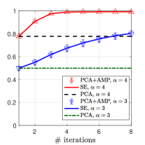
(a) Square, MP.

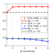
(b) Square, uniform.

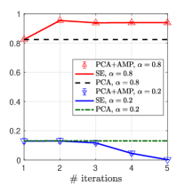
(c) Rectangular, left.

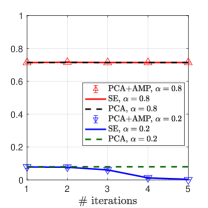
(d) Rectangular, right.

Figure 1: Comparison between AMP with PCA initialization and the related state evolution (SE). The plots show the normalized squared correlation between iterate and signal, as a function of the number of iterations.

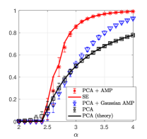
(a) Square, MP.

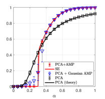
(b) Square, uniform.

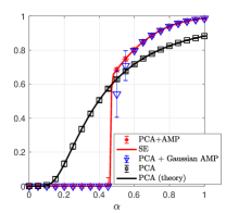
(c) Rectangular, left.

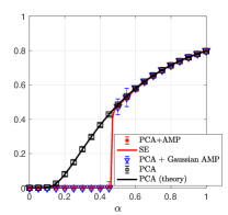
(d) Rectangular, right.

Figure 2: Comparison between AMP with PCA initialization and the PCA method alone. The plots show the normalized squared correlation between the signal and the estimate (PCA, or AMP+PCA), as a function of $\alpha$.

Figure 1 compares the performance between the proposed AMP algorithm with PCA initialization (PCA+AMP) and the theoretical predictions of state evolution (SE), for two different values of $\alpha$. On the $x$-axis, we have the number of iterations of AMP, and on the $y$-axis the normalized squared correlation between the iterate and the signal. As a reference, we also plot the performance of PCA as a horizontal line. We observe an excellent agreement of AMP with state evolution, even in the settings (b)-(c)-(d) where the free cumulants (resp. rectangular free cumulants) are alternating in sign. This supports our conjecture that Theorems 1-2 hold for more general noise distributions.

In Figure 2, we run PCA+AMP until the algorithm converges, and we compare the results with (i) the AMP with PCA initialization developed in [MV21b] which assumes that the noise matrix is Gaussian (with the correct variance), and (ii) the PCA method alone, as a function of the SNR $\alpha$. For Marchenko-Pastur noise (setting (a)), PCA+AMP always improves upon the PCA initialization. However, this is not the case when the eigenvalues/singular values of the noise are uniformly distributed (settings (b), (c) and (d)). In fact, we observe a phase transition phenomenon: below a certain critical $\alpha$, AMP converges to a trivial fixed point at $0$, while PCA shows positive correlation with the signal; above the critical $\alpha$, PCA+AMP is no worse than PCA. This is due to the sub-optimal choice of ${\sf u}_{t}$; recall the discussion on p.3.1. We observe no improvement for the estimation of the right singular vector (setting (d)), as the prior of ${\boldsymbol{v}}^{*}$ is Gaussian, in which case we expect the PCA estimate to be optimal. The interesting behavior demonstrated in Figure 2 motivates the study of the optimal choice for ${\sf u}_{t},{\sf v}_{t}$ in future work. We also note that, in settings (c)-(d), $\tilde{\alpha}_{\rm s}=0$, which means that the PCA estimator has non-zero correlation with the signal for all $\alpha>0$. However, for $\alpha<0.1$, this correlation remains rather small. Finally, we highlight that our proposed rotationally invariant PCA+AMP always improves upon the Gaussian PCA+AMP. In general, this performance gap will be significant unless the sequence of free cumulants $\kappa_{k}^{\infty}$ ($\kappa_{2k}^{\infty}$ in the rectangular case) decays quickly. For Marchenko-Pastur noise, the free cumulants are all equal, and thus the performance gap is significant. If the eigenvalues/singular values of the noise are uniform, then the sequence of free cumulants decays rapidly and the performance gap is small.

5 Proof Sketch: Symmetric Square Matrices

We consider the following artificial AMP algorithm, whose iterates are denoted by ${\tilde{\boldsymbol{u}}}^{t},{\tilde{\boldsymbol{f}}}^{t}$ for $t\geq 1$. We initialize with $\tilde{{\boldsymbol{u}}}^{1}=\rho_{\alpha}{\boldsymbol{u}}^{*}+\sqrt{1-\rho_{\alpha}^{2}}\,{\boldsymbol{n}}$ and ${\tilde{\boldsymbol{f}}}^{1}={\boldsymbol{X}}{\tilde{\boldsymbol{u}}}^{1}-\kappa_{1}{\tilde{\boldsymbol{u}}}^{1}$. Here, ${\boldsymbol{n}}$ is standard Gaussian and $\rho_{\alpha}$ is the normalized (limit) correlation of the PCA estimate given in (2.2). We note that this initialization is impractical, as it requires the knowledge of the unknown signal ${\boldsymbol{u}}^{*}$. However, this is not an issue since the artificial AMP serves only as a proof technique. (The true AMP (3.2) used for estimation uses the PCA initialization in (3.1).) The subsequent iterates of the artificial AMP are defined in two phases. In the first phase, which lasts up to iteration $(T+1)$, the functions defining the artificial AMP are chosen so that $\tilde{{\boldsymbol{u}}}^{T+1}$ is closely aligned with the eigenvector ${\boldsymbol{u}}_{{\rm PCA}}$ as $T\to\infty$. In the second phase, the functions are chosen to match those in the true AMP.

The artificial AMP initialization $\tilde{{\boldsymbol{u}}}^{1}$ is chosen such that it has non-zero asymptotic correlation with the signal ${\boldsymbol{u}}^{*}$. Indeed, when the signal prior has zero mean, a random initialization (independent of ${\boldsymbol{u}}^{*}$) would be asymptotically uncorrelated with the signal; consequently, the first phase of the artificial AMP would get stuck at a trivial fixed point and the iterates would not be guaranteed to converge to the principal eigenvector. We ensure that this does not happen by defining the initialization $\tilde{{\boldsymbol{u}}}^{1}$ to be a linear combination of the signal and Gaussian noise.

First phase.

For $2\leq t\leq(T+1)$, the artificial AMP iterates are

$$\begin{split}{\tilde{\boldsymbol{u}}}^{t}=\tilde{{\boldsymbol{f}}}^{t-1}/\alpha,\qquad{\tilde{\boldsymbol{f}}}^{t}={\boldsymbol{X}}\tilde{{\boldsymbol{u}}}^{t}-\sum_{i=1}^{t}\tilde{{\sf b}}_{t,i}\tilde{{\boldsymbol{u}}}^{i},\end{split}$$ (5.1)

where $\tilde{{\sf b}}_{t,t-j}=\kappa_{j+1}\alpha^{-j}$, for $(t-j)\in[1,t]$. We claim that, for sufficiently large $T$, $\tilde{{\boldsymbol{u}}}^{T+1}$ approaches the PCA estimate ${\boldsymbol{u}}_{\rm PCA}$, that is, $\lim_{T\to\infty}\lim_{n\to\infty}\frac{1}{\sqrt{n}}\|\tilde{{\boldsymbol{u}}}^{T+1}-\sqrt{n}{\boldsymbol{u}}_{\rm PCA}\|\,=\,0.$ This result is proved in Lemma B.31 in Appendix B.3. We give a heuristic sanity check here. Assume that the iterate $\tilde{{\boldsymbol{u}}}^{T+1}$ converges to a limit $\tilde{{\boldsymbol{u}}}^{\infty}$ in the sense that $\lim_{T\to\infty}\lim_{n\to\infty}\frac{1}{\sqrt{n}}\|\tilde{{\boldsymbol{u}}}^{T+1}-\tilde{{\boldsymbol{u}}}^{\infty}\|=0$. Then, from (5.1), the limit $\tilde{{\boldsymbol{u}}}^{\infty}$ satisfies

$$\tilde{{\boldsymbol{u}}}^{\infty}=\frac{1}{\alpha}{\boldsymbol{X}}\tilde{{\boldsymbol{u}}}^{\infty}-\sum_{i=1}^{\infty}\kappa_{i}\left(\frac{1}{\alpha}\right)^{i}\tilde{{\boldsymbol{u}}}^{\infty}\Longleftrightarrow\Bigg{(}\alpha+\sum_{i=1}^{\infty}\kappa_{i}\left(\frac{1}{\alpha}\right)^{i-1}\Bigg{)}\tilde{{\boldsymbol{u}}}^{\infty}={\boldsymbol{X}}\tilde{{\boldsymbol{u}}}^{\infty},$$ (5.2)

which means that $\tilde{{\boldsymbol{u}}}^{\infty}$ is an eigenvector of ${\boldsymbol{X}}$. Furthermore, by using known identities in free probability (see (A.4) and (A.6)), the eigenvalue $\alpha+\sum_{i=1}^{\infty}\kappa_{i}\left(\frac{1}{\alpha}\right)^{i-1}$ can be re-written as $G^{-1}(1/\alpha)$. Recall that, for $\alpha>\alpha_{\rm s}$, ${\boldsymbol{X}}$ exhibits a spectral gap and its largest eigenvalue converges to $G^{-1}(1/\alpha)$. Thus, ${\boldsymbol{u}}^{\infty}$ must be aligned with the principal eigenvector of ${\boldsymbol{X}}$, as desired.

A key step in our analysis is to show that, as $T\to\infty$, the state evolution of the artificial AMP in the first phase has the unique fixed point $(\tilde{\mu}=\alpha\rho_{\alpha},\tilde{\sigma}=\alpha^{2}(1-\rho_{\alpha}^{2}))$. This is established in Lemma B.7 proved in Appendix B.2. The proof follows the approach developed in Section 7 of [Fan20]. However, the analysis of [Fan20] requires that $\alpha$ is sufficiently large, while our result holds for all $\alpha>\alpha_{\rm s}$. Our idea is to exploit the expression of the limit correlation between the PCA estimate and the signal. In particular, we prove that, when the PCA estimate is correlated with the signal, state evolution is close to a limit map which is a contraction. The price to pay for this approach is the requirement that the free cumulants are non-negative.

Second phase.

The second phase of the artificial AMP is designed so that its iterates $({\tilde{\boldsymbol{u}}}^{T+k},{\tilde{\boldsymbol{f}}}^{T+k})$ are close to $({\boldsymbol{u}}^{k},{\boldsymbol{f}}^{k})$, for $k\geq 2$. For $t\geq(T+2)$, the artificial AMP computes:

$${\tilde{\boldsymbol{u}}}^{t}={\sf u}_{t-T}({\tilde{\boldsymbol{f}}}^{t-1}),\qquad{\tilde{\boldsymbol{f}}}^{t}={\boldsymbol{X}}{\tilde{\boldsymbol{u}}}^{t}-\sum_{i=1}^{t}{\tilde{\sf b}}_{t,i}{\tilde{\boldsymbol{u}}}^{i}.$$ (5.3)

Here, the functions $\{u_{k}\}_{k\geq 2}$, are the ones used in the true AMP (3.2). The coefficients $\{{\tilde{\sf b}}_{t,i}\}$ for $t\geq(T+2)$ are given by:

$${\tilde{\sf b}}_{tt}=\kappa_{1},\quad{\tilde{\sf b}}_{t,t-j}=\kappa_{j+1}\left(\frac{1}{\alpha}\right)^{(T+1-(t-j))_{+}}\prod_{i=\max\{t-j+1,T+2\}}^{t}\langle{\sf u}^{\prime}_{i-T}({\tilde{\boldsymbol{f}}}^{i-1})\rangle,\quad(t-j)\in[1,t-1].$$ (5.4)

Since the artificial AMP is initialized with ${\tilde{\boldsymbol{u}}}^{1}$ that is correlated with ${\boldsymbol{u}}^{*}$ and independent of the noise matrix ${\boldsymbol{W}}$, a state evolution result for it can be obtained directly from [Fan20, Theorem 1.1]. We then show in Lemma B.8 in Appendix B.4 that the second phase iterates in (5.3) are close to the true AMP iterates in (3.2), and that their state evolution parameters are also close. This result yields Theorem 1, as shown in Appendix B.5. The complete proof of Theorem 2 (rectangular case) is given in Appendix C. We describe the artificial AMP for this case along with a proof sketch in Appendix C.1.

Appendix A Free Probability Background

A.1 Symmetric Square Matrices

Let $X$ be a random variable of finite moments of all orders, and denote its moments by $m_{k}=\mathbb{E}\{X^{k}\}$. In this paper, $X$ represents either the empirical eigenvalue distribution of the noise matrix ${\boldsymbol{W}}\in\mathbb{R}^{n\times n}$, or its limit law $\Lambda$ (in the latter case, the moments and free cumulants are denoted by $\{m_{k}^{\infty}\}_{k\geq 1}$ and $\{\kappa_{k}^{\infty}\}_{k\geq 1}$, respectively). For the model (1.1), note that the empirical eigenvalue distribution of ${\boldsymbol{W}}$ coincides with the empirical eigenvalue distribution of ${\boldsymbol{X}}$ after excluding the largest eigenvalue of ${\boldsymbol{X}}$, since we consider the case $\alpha>\alpha_{\rm s}$. The free cumulants $\{\kappa_{k}\}_{k\geq 1}$ of $X$ are defined recursively by the moment-cumulant relations

$$m_{k}=\sum_{\pi\in{\rm NC}(k)}\prod_{S\in\pi}\kappa_{|S|},$$ (A.1)

where ${\rm NC}(k)$ is the set of all non-crossing partitions of $\{1,\ldots,k\}$, and $|S|$ denotes the cardinality of $S$. Furthermore, by exploiting the connection between the formal power series with coefficients $\{m_{k}\}_{k\geq 1}$ and $\{\kappa_{k}\}_{k\geq 1}$, each free cumulant $\kappa_{k}$ can be computed from $m_{1},\ldots,m_{k}$ and $\kappa_{1},\ldots,\kappa_{k-1}$ as [Nov14, Section 2.5]

$$\kappa_{k}=m_{k}-[z^{k}]\sum_{j=1}^{k-1}\kappa_{j}\left(z+m_{1}z^{2}+m_{2}z^{3}+\cdots+m_{k-1}z^{k}\right)^{j},$$ (A.2)

where $[z^{k}](q(z))$ denotes the coefficient of $z^{k}$ in the polynomial $q(z)$.

Consider now the random variable $\Lambda$ representing the limiting spectral distribution of ${\boldsymbol{W}}$, and recall that $b<\infty$ denotes the supremum of the support of $\Lambda$. Then, for $z>b$, the Cauchy transform $G(z)$ of $\Lambda$ is given by

$$G(z)=\mathbb{E}\left\{\frac{1}{z-\Lambda}\right\}.$$ (A.3)

Another transform that will be useful in our analysis is the $R$-transform $R(z)$ of $\Lambda$, which can be defined by the convergent series:

$$R(z)=\sum_{i=0}^{\infty}\kappa_{i+1}^{\infty}z^{i},$$ (A.4)

where $\{\kappa^{\infty}_{k}\}_{k\geq 1}$ are the free cumulants of $\Lambda$. The derivative of the $R$-transform is denoted by $R^{\prime}(z)$ and given by

$$R^{\prime}(z)=\sum_{i=0}^{\infty}(i+1)\kappa_{i+2}^{\infty}z^{i}=\sum_{j=0}^{\infty}\sum_{k=0}^{\infty}\kappa_{j+k+2}z^{j+k},$$ (A.5)

where the second equality follows from a double-counting argument. The series in (A.4) and (A.5) are well-defined and converge to a finite value for $z<1/\alpha_{\rm s}$, where $\alpha_{\rm s}=1/G(b^{+})$ is the spectral threshold [BGN11]. The $R$-transform can also be expressed in terms of the Cauchy transform, see e.g. Theorem 12.7 of [NS06]:

$$R(z)=G^{-1}(z)-\frac{1}{z}.$$ (A.6)

By taking the derivative on both sides of (A.5), we have

$$R^{\prime}(z)=\frac{1}{G^{\prime}(G^{-1}(z))}+\frac{1}{z^{2}}.$$ (A.7)

If ${\boldsymbol{W}}$ follows a Marcenko-Pastur distribution (i.e., ${\boldsymbol{W}}=\frac{1}{n}{\boldsymbol{G}}_{n}{\boldsymbol{G}}_{n}^{\sf T}\in\mathbb{R}^{n\times n}$, where the entries of ${\boldsymbol{G}}_{n}\in\mathbb{R}^{n\times p}$ are i.i.d. standard Gaussian), then it is well known that $\kappa_{k}^{\infty}=c\triangleq p/n$ for $k\geq 1$, see e.g. [MS17, Chap. 2, Exercise 11]. This corresponds to the setting (a) in the numerical results of Section 4. If the eigenvalues of ${\boldsymbol{W}}$ are i.i.d. and uniformly distributed in the interval $[-1/2,1/2]$, the free cumulants $\kappa_{k}^{\infty}$ have also a simple form. In fact, by explicitly computing the expectation in (A.3), we have that

$$G(z)=\log\frac{2z+1}{2z-1}.$$ (A.8)

Thus, by applying (A.6), we deduce that

$$R(z)=\frac{1}{2}\coth\left(\frac{z}{2}\right)-\frac{1}{z}.$$ (A.9)

By comparing the series expansion (A.4) with that of the hyperbolic cotangent, we conclude that

$$\kappa_{k}=\begin{cases}0,\quad\quad\mbox{ if $k$ is odd,}\vspace{.5em}\\ \displaystyle\frac{B_{k}}{k!},\,\,\quad\mbox{if $k$ is even,}\\ \end{cases}$$ (A.10)

where $B_{k}$ denotes the $k$-th Bernoulli number. This corresponds to the setting (b) in the numerical results of Section 4.

A.2 Rectangular Matrices

Let $X$ be a random variable of finite moments of all orders, and denote its even moments by $m_{2k}=\mathbb{E}\{X^{2k}\}$. In this paper, $X^{2}$ represents either the empirical eigenvalue distribution of ${\boldsymbol{W}}{\boldsymbol{W}}^{\sf T}\in\mathbb{R}^{m\times m}$, or its limit law $\Lambda^{2}$ (in the latter case, the moments and rectangular free cumulants are denoted by $\{m_{2k}^{\infty}\}_{k\geq 1}$ and $\{\kappa_{2k}^{\infty}\}_{k\geq 1}$, respectively). For the model (1.2), note that the empirical eigenvalue distribution of ${\boldsymbol{W}}{\boldsymbol{W}}^{\sf T}$ coincides with the empirical eigenvalue distribution of ${\boldsymbol{X}}{\boldsymbol{X}}^{\sf T}$ after excluding the largest eigenvalue of ${\boldsymbol{X}}{\boldsymbol{X}}^{\sf T}$, since we consider the case $\tilde{\alpha}>\tilde{\alpha}_{\rm s}$. The rectangular free cumulants $\{\kappa_{2k}\}_{k\geq 1}$ of $X$ are defined recursively by the moment-cumulant relations [BG09, Section 3]

$$m_{2k}=\gamma\sum_{\pi\in{\rm NC}^{\prime}(2k)}\prod_{\begin{subarray}{c}S\in\pi\\ \min S\,\,\,\mbox{\scriptsize is odd}\end{subarray}}\kappa_{|S|}\prod_{\begin{subarray}{c}S\in\pi\\ \min S\,\,\,\mbox{\scriptsize is even}\end{subarray}}\kappa_{|S|},$$ (A.11)

where ${\rm NC}^{\prime}(2k)$ is the set of non-crossing partitions $\pi$ of $\{1,\ldots,2k\}$ such that each set $S\in\pi$ has even cardinality. Furthermore, by exploiting the connection between the formal power series with coefficients $\{m_{2k}\}_{k\geq 1}$ and $\{\kappa_{2k}\}_{k\geq 1}$, each rectangular free cumulant $\kappa_{2k}$ can be computed from $m_{2},\ldots,m_{2k}$ and $\kappa_{2},\ldots,\kappa_{2(k-1)}$ as [BG09, Lemma 3.4]

$$\kappa_{2k}=m_{2k}-[z^{k}]\sum_{j=1}^{k-1}\kappa_{2j}\left(z(\gamma M(z)+1)(M(z)+1)\right)^{j},$$ (A.12)

where $M(z)=\sum_{k=1}^{\infty}m_{2k}z^{k}$ and $[z^{k}](q(z))$ denotes again the coefficient of $z^{k}$ in the polynomial $q(z)$.

Consider now the random variable $\Lambda$ representing the limiting distribution of the singular values of ${\boldsymbol{W}}$, and recall that $b<\infty$ denotes the supremum of the support of $\Lambda$. Then, for $z>b$, the $D$-transform $D(z)$ of $\Lambda$ is given by

$$D(z)=\phi(z)\cdot\bar{\phi}(z),$$ (A.13)

where

$$\phi(z)=\mathbb{E}\left\{\frac{z}{z^{2}-\Lambda^{2}}\right\},\quad\bar{\phi}(z)=\gamma\phi(z)+\frac{1-\gamma}{z}.$$ (A.14)

Another transform that will be useful in our analysis is the rectangular $R$-transform $R(z)$ of $\Lambda$, which can be defined by the convergent series:

$$R(z)=\sum_{i=1}^{\infty}\kappa_{2i}^{\infty}z^{i},$$ (A.15)

where $\{\kappa^{\infty}_{2k}\}_{k\geq 1}$ are the rectangular free cumulants of $\Lambda$. The derivative of the rectangular $R$-transform is denoted by $R^{\prime}(z)$ and given by

$$R^{\prime}(z)=\sum_{i=0}^{\infty}(i+1)\kappa_{2(i+1)}^{\infty}z^{i}=\sum_{j=0}^{\infty}\sum_{k=0}^{\infty}\kappa_{2(j+k+1)}z^{j+k},$$ (A.16)

where the second equality follows from a double-counting argument. By combining (A.15) and (A.16), we also obtain the useful identities

$$\sum_{j=0}^{\infty}\sum_{k=0}^{\infty}\kappa_{2(j+k+2)}z^{j+k+2}=zR^{\prime}(z)-R(z),$$ (A.17)

$$\sum_{i=0}^{\infty}(i+1)\kappa_{2(i+2)}^{\infty}z^{i}=z^{-1}R^{\prime}(z)-z^{-2}R(z).$$ (A.18)

The series in (A.15)-(A.18) are well-defined and converge to a finite value for $z<1/(\tilde{\alpha}_{\rm s})^{2}$, where $\tilde{\alpha}_{\rm s}=1/\sqrt{D(b^{+})}$ is the spectral threshold [BGN12]. The rectangular $R$-transform can also be expressed in terms of the $D$-transform, see e.g. [BGN12, Section 2.5]:

$$\gamma R^{2}(z)+(\gamma+1)R(z)+1=z(D^{-1}(z))^{2}.$$ (A.19)

Appendix B Proof of Theorem 1

This appendix is organized as follows. In Appendix B.1, we present the state evolution recursion associated to the artificial AMP iteration defined in (5.1) and (5.3). In Appendix B.2, we prove that the first phase of this state evolution admits a unique fixed point. Using this fact, in Appendix B.3, we prove that the artificial AMP iterate at the end of the first phase approaches the PCA estimator. Then, in Appendix B.4, we show that (i) the iterates in the second phase of the artificial AMP are close to the true AMP iterates, and (ii) the related state evolution parameters also remain close. Finally, in Appendix B.5, we give the proof of Theorem 1.

B.1 State Evolution for the Artificial AMP

Consider the artificial AMP iteration defined in (5.1) and (5.3), with initialization

$$\tilde{{\boldsymbol{u}}}^{1}=\rho_{\alpha}{\boldsymbol{u}}^{*}+\sqrt{1-\rho_{\alpha}^{2}}{\boldsymbol{n}},\qquad{\tilde{\boldsymbol{f}}}^{1}={\boldsymbol{X}}{\tilde{\boldsymbol{u}}}^{1}-\kappa_{1}{\tilde{\boldsymbol{u}}}^{1}.$$ (B.1)

Then, its associated state evolution recursion is expressed in terms of a sequence of mean vectors $\tilde{{\boldsymbol{\mu}}}_{K}=(\tilde{\mu}_{t})_{t\in[0,K]}$ and covariance matrices $\tilde{{\boldsymbol{\Sigma}}}_{K}=(\tilde{\sigma}_{s,t})_{s,t\in[0,K]}$ defined recursively as follows. We initialize with

$$\tilde{\mu}_{0}=\alpha\rho_{\alpha},\qquad\tilde{\sigma}_{0,0}=\alpha^{2}(1-\rho_{\alpha}^{2}),\quad\tilde{\sigma}_{0,t}=\tilde{\sigma}_{t,0}=0,\quad\mbox{ for }t\geq 1.$$ (B.2)

Given $\tilde{{\boldsymbol{\mu}}}_{K}$ and $\tilde{{\boldsymbol{\Sigma}}}_{K}$, let

$$(\tilde{F_{0}},\ldots,\tilde{F}_{K})=\tilde{{\boldsymbol{\mu}}}_{K}U_{*}+(\tilde{Z}_{0},\ldots,\tilde{Z}_{K}),\quad\text{ where }\ (\tilde{Z}_{0},\ldots,\tilde{Z}_{K})\sim\mathcal{N}(\boldsymbol{0},\tilde{{\boldsymbol{\Sigma}}}_{K}),\quad\text{ and }$$

$$\tilde{U}_{t}={\tilde{\sf u}}_{t}(\tilde{F}_{t-1}),\quad\text{ where }\ {\tilde{\sf u}}_{t}(x)=\begin{cases}x/\alpha,&1\leq t\leq T+1,\\ {\sf u}_{t-T}(x),&t\geq T+2.\end{cases}$$ (B.3)

Then, the entries of $\tilde{{\boldsymbol{\mu}}}_{K+1}$ are given by $\tilde{\mu}_{t}=\alpha{\mathbb{E}}\{\tilde{U}_{t}U_{*}\}$ (for $t\in[1,K+1]$), and the entries of $\tilde{{\boldsymbol{\Sigma}}}_{K+1}$ (for $s,t\in[1,K+1]$) are given by

$$\tilde{\sigma}_{s,t} =\sum_{j=0}^{s-1}\sum_{k=0}^{t-1}\kappa_{j+k+2}^{\infty}\left(\prod_{i=s-j+1}^{s}{\mathbb{E}}\{{\tilde{\sf u}}^{\prime}_{i}(\tilde{F}_{i-1})\}\right)\left(\prod_{i=t-k+1}^{t}{\mathbb{E}}\{{\tilde{\sf u}}^{\prime}_{i}(\tilde{F}_{i-1})\}\right){\mathbb{E}}\{\tilde{U}_{s-j}\tilde{U}_{t-k}\}.$$ (B.4)

Proposition B.1 (State evolution for artificial AMP – symmetric square matrices).

Consider the setting of Theorem 1, the artificial AMP iteration described in (5.1) and (5.3) with the initialization given in (B.1), and the corresponding state evolution parameters defined in (B.2)-(B.4). Then, for $t\geq 1$ and any PL($2$) function $\psi:\mathbb{R}^{2t+2}\to\mathbb{R}$, the following holds almost surely:

$$\lim_{n\to\infty}\frac{1}{n}\sum_{i=1}^{n}\psi(u^{*}_{i},\tilde{u}^{1}_{i},\ldots,\tilde{u}^{t+1}_{i},\tilde{f}^{1}_{i},\ldots\tilde{f}^{t}_{i})={\mathbb{E}}\left\{\psi(U_{*},\tilde{U}_{1},\ldots,\tilde{U}_{t+1},\tilde{F}_{1},\ldots,\tilde{F}_{t})\right\}.$$ (B.5)

The proposition follows directly from Theorem 1.1 in [Fan20] since the initialization $\tilde{{\boldsymbol{u}}}^{1}$ of the artificial AMP is independent of ${\boldsymbol{W}}$.

B.2 Fixed Point of State Evolution for the First Phase

From (B.2)-(B.4), we note that the state evolution recursion for the first phase $(t\in[1,T+1])$ has the following form:

$$\begin{split}\tilde{\mu}_{t}&=\alpha\rho_{\alpha},\quad\mbox{ for }t\in[1,T+1],\\ \tilde{\sigma}_{s,t}&=\sum_{j=0}^{s-1}\sum_{k=0}^{t-1}\kappa_{j+k+2}^{\infty}\left(\frac{1}{\alpha}\right)^{j+k+2}\left((\alpha\rho_{\alpha})^{2}+\tilde{\sigma}_{s-j-1,t-k-1}\right),\quad\mbox{ for }s,t\in[1,T+1].\end{split}$$ (B.6)

In this section, we prove the following result concerning the fixed point of the recursion (B.6).

Lemma B.2 (Fixed point of state evolution for first phase – Square matrices).

Consider the state evolution recursion for the first phase given by (B.6), initialized according to (B.2). Assume that $\kappa_{i}^{\infty}\geq 0$ for all $i\geq 2$, and that $\alpha>\alpha_{\rm s}$. Pick any $\xi<1$ such that $\alpha\xi>\alpha_{\rm s}$. Then,

$$\lim_{T\to\infty}\max_{s,t\in[0,T]}\xi^{\max(s,t)}|\tilde{\sigma}_{T+1-s,T+1-t}-\alpha^{2}(1-\rho_{\alpha}^{2})|=0.$$ (B.7)

To prove the claim, we consider the space of infinite matrices ${\boldsymbol{x}}=(x_{s,t}:s,t\leq 0)$ indexed by the non-positive integers and equipped with the weighted $\ell_{\infty}$-norm:

$$\|{\boldsymbol{x}}\|_{\xi}=\sup_{s,t\leq 0}\xi^{\max(|s|,|t|)}|x_{s,t}|.$$ (B.8)

We define $\mathcal{X}=\{{\boldsymbol{x}}:\|{\boldsymbol{x}}\|_{\xi}<\infty\}$, and note that $\mathcal{X}$ is complete under $\|\cdot\|_{\xi}$. For any compact set $I\subset\mathbb{R}$, we also define

$$\mathcal{X}_{I}=\{{\boldsymbol{x}}:x_{s,t}\in I\mbox{ for all }s,t\leq 0\}\subset\mathcal{X}.$$ (B.9)

Then, $\mathcal{X}_{I}$ is closed in $\mathcal{X}$ and therefore it is also complete under $\|\cdot\|_{\xi}$. We embed the matrix ${\tilde{\boldsymbol{\Sigma}}}_{\bar{T}}$ as an element ${\boldsymbol{x}}\in\mathcal{X}$ with the following coordinate identification:

$$\begin{split}\tilde{\sigma}_{s,t}&=x_{s-\bar{T},t-\bar{T}},\\ x_{s,t}&=0,\quad\mbox{ if }s<-\bar{T}\mbox{ or }t<-\bar{T}.\end{split}$$

The idea is to approximate the map ${\tilde{\boldsymbol{\Sigma}}}_{\bar{T}-1}\mapsto{\tilde{\boldsymbol{\Sigma}}}_{\bar{T}}$ with the limit map $h^{\Sigma}$ defined as

$$h_{s,t}^{\Sigma}({\boldsymbol{x}})=\sum_{j=0}^{\infty}\sum_{k=0}^{\infty}\kappa_{j+k+2}^{\infty}\left(\frac{1}{\alpha}\right)^{j+k+2}\left((\alpha\rho_{\alpha})^{2}+x_{s-j,t-k}\right).$$ (B.10)

The map $h^{\Sigma}$ has a similar structure to the embedding of the map ${\tilde{\boldsymbol{\Sigma}}}_{\bar{T}-1}\mapsto{\tilde{\boldsymbol{\Sigma}}}_{\bar{T}}$ into $\mathcal{X}$. However, comparing (B.6) and (B.10), we highlight two important differences. First, the indices of $x_{s-j,t-k}$ are shifted with respect to the indices of $\tilde{\sigma}_{s-j-1,t-k-1}$. This difference is purely technical and it simplifies the proof of the subsequent Lemma B.6, which shows that $h^{\Sigma}$ is close to the map ${\tilde{\boldsymbol{\Sigma}}}_{\bar{T}-1}\mapsto{\tilde{\boldsymbol{\Sigma}}}_{\bar{T}}$. Second, the map $h^{\Sigma}$ is fixed, in the sense that it does not depend on $s,t$. In fact, note that the sums over $j$ and $k$ run from $0$ to $\infty$ in (B.10). This is in contrast with (B.6) where the two sums run until $j=s-1$ and $k=t-1$.

The approach of approximating the state evolution map with a fixed limit map was first developed in [Fan20]. The key difference is that, in [Fan20], it is assumed that $\alpha$ is sufficiently large, which allows to simplify the analysis. On the contrary, our result holds for all $\alpha>\alpha_{\rm s}$, $\alpha_{\rm s}$ being the spectral threshold for PCA. This is because of two main reasons. First, the expressions for the state evolution recursion are simplified by considering linear denoisers in the first phase of the artificial AMP. Second, we crucially exploit the form (and the strict positivity) of the correlation between the signal and the PCA estimate, in order to prove that the limit map (B.10) is a contraction (cf. (B.14) in Lemma B.5).

First, we show that $h^{\Sigma}(\mathcal{X}_{I^{*}})\subseteq\mathcal{X}_{I^{*}}$ for a suitably defined compact set $I^{*}$.

Lemma B.3 (Image of limit map – Square matrices).

Consider the map $h^{\Sigma}$ defined in (B.10). Assume that $\kappa_{i}^{\infty}\geq 0$ for all $i\geq 2$, and that $\alpha>\alpha_{\rm s}$. Then, there exists $I^{*}=[-a^{*},a^{*}]$ such that, if ${\boldsymbol{x}}\in\mathcal{X}_{I^{*}}$, then $h^{\Sigma}({\boldsymbol{x}})\in\mathcal{X}_{I^{*}}$.

Proof.

Let ${\boldsymbol{x}}\in\mathcal{X}_{I^{*}}$. Then, the following chain of inequalities holds:

$$\begin{split}|h_{s,t}^{\Sigma}({\boldsymbol{x}})|&\stackrel{{\scriptstyle\mathclap{\mbox{\footnotesize(a)}}}}{{=}}\left|\rho_{\alpha}^{2}R^{\prime}\left(\frac{1}{\alpha}\right)+\sum_{j=0}^{\infty}\sum_{k=0}^{\infty}\kappa_{j+k+2}^{\infty}\left(\frac{1}{\alpha}\right)^{j+k+2}x_{s-j,t-k}\right|\\ &\stackrel{{\scriptstyle\mathclap{\mbox{\footnotesize(b)}}}}{{\leq}}\rho_{\alpha}^{2}\left|R^{\prime}\left(\frac{1}{\alpha}\right)\right|+\sum_{j=0}^{\infty}\sum_{k=0}^{\infty}\kappa_{j+k+2}^{\infty}\left(\frac{1}{\alpha}\right)^{j+k+2}|x_{s-j,t-k}|\\ &\stackrel{{\scriptstyle\mathclap{\mbox{\footnotesize(c)}}}}{{\leq}}\rho_{\alpha}^{2}\left|R^{\prime}\left(\frac{1}{\alpha}\right)\right|+a^{*}R^{\prime}\left(\frac{1}{\alpha}\right)\left(\frac{1}{\alpha}\right)^{2}.\end{split}$$

Here, (a) follows from (B.10) and (A.5); (b) follows from the hypothesis that $\kappa_{i}^{\infty}\geq 0$ for $i\geq 2$; and (c) uses again (A.5) and the fact that ${\boldsymbol{x}}\in\mathcal{X}_{I^{*}}$.

Now, recall from (2.2) that above the spectral threshold, namely, when $\alpha>\alpha_{\rm s}$, the PCA estimator ${\boldsymbol{u}}_{\rm PCA}$ has strictly positive correlation with the signal ${\boldsymbol{u}}^{*}$:

$$\frac{\langle{\boldsymbol{u}}_{\rm PCA},{\boldsymbol{u}}^{*}\rangle^{2}}{n}\stackrel{{\scriptstyle\mathclap{\mbox{\footnotesize a.s.}}}}{{\longrightarrow}}\rho_{\alpha}^{2}=\frac{-1}{\alpha^{2}G^{\prime}(G^{-1}(1/\alpha))},$$

which immediately implies that

$$\frac{1}{\alpha^{2}G^{\prime}(G^{-1}\left(\frac{1}{\alpha}\right))}<0.$$ (B.11)

Thus, by combining (B.11) with (A.7), we deduce that

$$R^{\prime}\left(\frac{1}{\alpha}\right)\left(\frac{1}{\alpha}\right)^{2}<1.$$ (B.12)

Hence, as $R^{\prime}\left(\frac{1}{\alpha}\right)<\infty$, there exists an $a^{*}$ such that

$$\rho_{\alpha}^{2}\left|R^{\prime}\left(\frac{1}{\alpha}\right)\right|+a^{*}R^{\prime}\left(\frac{1}{\alpha}\right)\left(\frac{1}{\alpha}\right)^{2}\leq a^{*},$$

which implies the desired claim. ∎

Next, we compute a fixed point of $h^{\Sigma}$.

Lemma B.4 (Fixed point of limit map – Square matrices).

Consider the map $h^{\Sigma}$ defined in (B.10), and let ${\boldsymbol{x}}^{*}=(x^{*}_{s,t}:s,t\leq 0)$ with $x^{*}_{s,t}=\alpha^{2}(1-\rho_{\alpha}^{2})$. Assume that $\alpha>\alpha_{\rm s}$. Then, ${\boldsymbol{x}}^{*}$ is a fixed point of $h^{\Sigma}$.

Proof.

Note that, for $x=1/\alpha$, the power series expansion (A.5) of $R^{\prime}$ converges to a finite limit as $\alpha>\alpha_{\rm s}$. Hence, by using the definition (B.10), we have that

$$h_{s,t}^{\Sigma}({\boldsymbol{x}}^{*})=R^{\prime}\left(\frac{1}{\alpha}\right).$$

Then, the claim follows from (A.7) and the definition $\rho_{\alpha}=\sqrt{\frac{-1}{\alpha^{2}G^{\prime}(G^{-1}(1/\alpha))}}$, which together show that $R^{\prime}\left(\frac{1}{\alpha}\right)=\alpha^{2}(1-\rho_{\alpha}^{2})$. ∎

Let $I^{*}$ be such that $h^{\Sigma}:\mathcal{X}_{I^{*}}\to\mathcal{X}_{I^{*}}$ (the existence of such a set $I^{*}$ is guaranteed by Lemma B.3). Then, the next step is to show that $h^{\Sigma}:\mathcal{X}_{I^{*}}\to\mathcal{X}_{I^{*}}$ is a contraction. We remark that, by the Banach fixed point theorem, this result implies that the fixed point ${\boldsymbol{x}}^{*}$ defined in Lemma B.4 is unique.

Lemma B.5 (Limit map is a contraction).

Consider the map $h^{\Sigma}:\mathcal{X}_{I^{*}}\to\mathcal{X}_{I^{*}}$ defined in (B.10) and where $I^{*}$ is given by Lemma B.3. Assume that $\kappa_{i}^{\infty}\geq 0$ for all $i\geq 2$, and let $\xi<1$ be such that $\alpha\xi>\alpha_{\rm s}$. Then, for any ${\boldsymbol{x}},{\boldsymbol{y}}\in\mathcal{X}_{I^{*}}$,

$$\|h^{\Sigma}({\boldsymbol{x}})-h^{\Sigma}({\boldsymbol{y}})\|_{\xi}\leq R^{\prime}\left(\frac{1}{\xi\alpha}\right)\left(\frac{1}{\xi\alpha}\right)^{2}\|{\boldsymbol{x}}-{\boldsymbol{y}}\|_{\xi},$$ (B.13)

where

$$R^{\prime}\left(\frac{1}{\xi\alpha}\right)\left(\frac{1}{\xi\alpha}\right)^{2}<1.$$ (B.14)

Proof.

First of all, for any $s,t\leq 0$, we have that

$$\begin{split}|h_{s,t}^{\Sigma}({\boldsymbol{x}})-h_{s,t}^{\Sigma}({\boldsymbol{y}})|&\stackrel{{\scriptstyle\mathclap{\mbox{\footnotesize(a)}}}}{{=}}\left|\sum_{j=0}^{\infty}\sum_{k=0}^{\infty}\kappa_{j+k+2}^{\infty}\left(\frac{1}{\alpha}\right)^{j+k+2}\left(x_{s-j,t-k}-y_{s-j,t-k}\right)\right|\\ &\stackrel{{\scriptstyle\mathclap{\mbox{\footnotesize(b)}}}}{{\leq}}\sum_{j=0}^{\infty}\sum_{k=0}^{\infty}\kappa_{j+k+2}^{\infty}\left(\frac{1}{\alpha}\right)^{j+k+2}|x_{s-j,t-k}-y_{s-j,t-k}|.\end{split}$$ (B.15)

Here, (a) follows from (B.10), and (b) follows from the hypothesis that $\kappa_{i}^{\infty}\geq 0$ for $i\geq 2$. Furthermore, we have that

$$|x_{s-j,t-k}-y_{s-j,t-k}|\leq\|{\boldsymbol{x}}-{\boldsymbol{y}}\|_{\xi}\xi^{-\max(|s-j|,|t-k|)}.$$ (B.16)

Thus, by using (B.15) and (B.16), we obtain

$$\begin{split}\|h^{\Sigma}({\boldsymbol{x}})-h^{\Sigma}({\boldsymbol{y}})\|_{\xi}&=\sup_{s,t\leq 0}\xi^{\max(|s|,|t|)}|h_{s,t}^{\Sigma}({\boldsymbol{x}})-h_{s,t}^{\Sigma}({\boldsymbol{y}})|\\ &\leq\sup_{s,t\leq 0}\xi^{\max(|s|,|t|)}\|{\boldsymbol{x}}-{\boldsymbol{y}}\|_{\xi}\sum_{j=0}^{\infty}\sum_{k=0}^{\infty}\kappa_{j+k+2}^{\infty}\left(\frac{1}{\alpha}\right)^{j+k+2}\xi^{-\max(|s-j|,|t-k|)}.\end{split}$$ (B.17)

Note that, as $\xi<1$,

$$\xi^{-\max(|s-j|,|t-k|)}\leq\xi^{-\max(|s|,|t|)-j-k-2},$$

which implies that the RHS of (B.17) is bounded above by

$$\|{\boldsymbol{x}}-{\boldsymbol{y}}\|_{\xi}\sum_{j=0}^{\infty}\sum_{k=0}^{\infty}\kappa_{j+k+2}^{\infty}\left(\frac{1}{\xi\alpha}\right)^{j+k+2}=R^{\prime}\left(\frac{1}{\xi\alpha}\right)\left(\frac{1}{\xi\alpha}\right)^{2}\|{\boldsymbol{x}}-{\boldsymbol{y}}\|_{\xi},$$ (B.18)

where the equality follows from (A.5). This shows that (B.13) holds. The proof of (B.14) follows the same argument as (B.12), since $\xi\alpha>\alpha_{\rm s}$. ∎

At this point, we show that the state evolution of ${\tilde{\boldsymbol{\Sigma}}}_{\bar{T}}$ can be approximated via the fixed map $h^{\Sigma}$.

Lemma B.6 (Limit map approximates state evolution map – Square matrices).

Consider the map $h^{\Sigma}:\mathcal{X}_{I^{*}}\to\mathcal{X}_{I^{*}}$ defined in (B.10), where $I^{*}$ is given by Lemma B.3. Assume that $\kappa_{i}^{\infty}\geq 0$ for all $i\geq 2$, and let $\xi<1$ be such that $\alpha\xi>\alpha_{\rm s}$. Then, for any ${\boldsymbol{x}}\in\mathcal{X}_{I^{*}}$,

$$\|{\tilde{\boldsymbol{\Sigma}}}_{\bar{T}}-h^{\Sigma}({\boldsymbol{x}})\|_{\xi}\leq R^{\prime}\left(\frac{1}{\xi\alpha}\right)\left(\frac{1}{\xi\alpha}\right)^{2}\|{\tilde{\boldsymbol{\Sigma}}}_{\bar{T}-1}-{\boldsymbol{x}}\|_{\xi}+F(\bar{T}),$$ (B.19)

where

$$\lim_{\bar{T}\to\infty}F(\bar{T})=0.$$ (B.20)

Proof.

Throughout the proof, we consider ${\tilde{\boldsymbol{\Sigma}}}_{\bar{T}},{\tilde{\boldsymbol{\Sigma}}}_{\bar{T}-1}$ as embedded in $\mathcal{X}$. First, we write

$$\begin{split}\|{\tilde{\boldsymbol{\Sigma}}}_{\bar{T}}-h^{\Sigma}({\boldsymbol{x}})\|_{\xi}&=\sup_{s,t\leq 0}\xi^{\max(|s|,|t|)}|({\tilde{\boldsymbol{\Sigma}}}_{\bar{T}})_{s,t}-h^{\Sigma}_{s,t}({\boldsymbol{x}})|\\ &=\max\Bigg{(}\sup_{\begin{subarray}{c}s,t\leq 0\\ \max(|s|,|t|)<\bar{T}\end{subarray}}\xi^{\max(|s|,|t|)}|({\tilde{\boldsymbol{\Sigma}}}_{\bar{T}})_{s,t}-h^{\Sigma}_{s,t}({\boldsymbol{x}})|,\\ &\hskip 50.00008pt\sup_{\begin{subarray}{c}s,t\leq 0\\ \max(|s|,|t|)\geq\bar{T}\end{subarray}}\xi^{\max(|s|,|t|)}|({\tilde{\boldsymbol{\Sigma}}}_{\bar{T}})_{s,t}-h^{\Sigma}_{s,t}({\boldsymbol{x}})|\Bigg{)},\end{split}$$ (B.21)

where $({\tilde{\boldsymbol{\Sigma}}}_{\bar{T}})_{s,t}=\tilde{\sigma}_{s+\bar{T},t+\bar{T}}$ if $s\geq-\bar{T}$ and $t\geq-\bar{T}$, and $({\tilde{\boldsymbol{\Sigma}}}_{\bar{T}})_{s,t}=0$ otherwise.

Let us look at the case $\max(|s|,|t|)<\bar{T}$, and define $I_{1}=\{(j,k):j\geq s+\bar{T}\mbox{ or }k\geq t+\bar{T}\}$. Then,

$$\begin{split}|({\tilde{\boldsymbol{\Sigma}}}_{\bar{T}})_{s,t}-h^{\Sigma}_{s,t}({\boldsymbol{x}})|&=\bigg{|}\sum_{j=0}^{s+\bar{T}-1}\sum_{k=0}^{t+\bar{T}-1}\kappa_{j+k+2}^{\infty}\left(\frac{1}{\alpha}\right)^{j+k+2}\left(\alpha^{2}\rho_{\alpha}^{2}+\tilde{\sigma}_{s-j+\bar{T}-1,t-k+\bar{T}-1}\right)\\ &\hskip 90.00014pt-\sum_{j=0}^{\infty}\sum_{k=0}^{\infty}\kappa_{j+k+2}^{\infty}\left(\frac{1}{\alpha}\right)^{j+k+2}\left(\alpha^{2}\rho_{\alpha}^{2}+x_{s-j,t-k}\right)\bigg{|}\\ &\leq\left|\sum_{j=0}^{s+\bar{T}-1}\sum_{k=0}^{t+\bar{T}-1}\kappa_{j+k+2}^{\infty}\left(\frac{1}{\alpha}\right)^{j+k+2}\left(\tilde{\sigma}_{s-j+\bar{T}-1,t-k+\bar{T}-1}-x_{s-j,t-k}\right)\right|\\ &\hskip 20.00003pt+\left|\sum_{j,k\in I_{1}}\kappa_{j+k+2}^{\infty}\left(\frac{1}{\alpha}\right)^{j+k+2}\left(\alpha^{2}\rho_{\alpha}^{2}+x_{s-j,t-k}\right)\right|:=T_{1}+T_{2}.\end{split}$$ (B.22)

The term $T_{1}$ can be upper bounded as follows:

$$\begin{split}T_{1}&\stackrel{{\scriptstyle\mathclap{\mbox{\footnotesize(a)}}}}{{\leq}}\sum_{j=0}^{s+\bar{T}-1}\sum_{k=0}^{t+\bar{T}-1}\kappa_{j+k+2}^{\infty}\left(\frac{1}{\alpha}\right)^{j+k+2}\left|\tilde{\sigma}_{s-j+\bar{T}-1,t-k+\bar{T}-1}-x_{s-j,t-k}\right|\\ &\leq\sum_{j=0}^{s+\bar{T}-1}\sum_{k=0}^{t+\bar{T}-1}\kappa_{j+k+2}^{\infty}\left(\frac{1}{\alpha}\right)^{j+k+2}\|{\tilde{\boldsymbol{\Sigma}}}_{\bar{T}-1}-{\boldsymbol{x}}\|_{\xi}\xi^{-\max(|s-j|,|t-k|)}\\ &\stackrel{{\scriptstyle\mathclap{\mbox{\footnotesize(b)}}}}{{\leq}}\sum_{j=0}^{s+\bar{T}-1}\sum_{k=0}^{t+\bar{T}-1}\kappa_{j+k+2}^{\infty}\left(\frac{1}{\xi\alpha}\right)^{j+k+2}\|{\tilde{\boldsymbol{\Sigma}}}_{\bar{T}-1}-{\boldsymbol{x}}\|_{\xi}\xi^{-\max(|s|,|t|)}\\ &\stackrel{{\scriptstyle\mathclap{\mbox{\footnotesize(c)}}}}{{\leq}}\sum_{j=0}^{\infty}\sum_{k=0}^{\infty}\kappa_{j+k+2}^{\infty}\left(\frac{1}{\xi\alpha}\right)^{j+k+2}\|{\tilde{\boldsymbol{\Sigma}}}_{\bar{T}-1}-{\boldsymbol{x}}\|_{\xi}\xi^{-\max(|s|,|t|)}\\ &\stackrel{{\scriptstyle\mathclap{\mbox{\footnotesize(d)}}}}{{=}}R^{\prime}\left(\frac{1}{\xi\alpha}\right)\left(\frac{1}{\xi\alpha}\right)^{2}\|{\tilde{\boldsymbol{\Sigma}}}_{\bar{T}-1}-{\boldsymbol{x}}\|_{\xi}\xi^{-\max(|s|,|t|)}.\end{split}$$ (B.23)

Here, (a) and (c) follows from the hypothesis that $\kappa_{i}^{\infty}\geq 0$ for $i\geq 2$; (b) uses that $\xi<1$; and (d) uses (A.5). The term $T_{2}$ can be upper bounded as follows:

$$\begin{split}T_{2}&\leq\left(\alpha^{2}\rho_{\alpha}^{2}+a^{*}\right)\sum_{j,k\in I_{1}}\kappa_{j+k+2}^{\infty}\left(\frac{1}{\alpha}\right)^{j+k+2}\\ &\leq\frac{\alpha^{2}\rho_{\alpha}^{2}+a^{*}}{\alpha^{2}}\sum_{i=-\max(|s|,|t|)+\bar{T}}^{\infty}\kappa_{i+2}^{\infty}(i+1)\left(\frac{1}{\alpha}\right)^{i},\end{split}$$ (B.24)

where the first inequality uses that ${\boldsymbol{x}}\in\mathcal{X}_{I^{*}}$ and the second inequality uses that, if $(j,k)\in I_{1}$, then $j+k\geq-\max(|s|,|t|)+\bar{T}$. By combining (B.22), (B.23) and (B.24), we obtain that

$$\begin{split}&\sup_{\begin{subarray}{c}s,t\leq 0\\ \max(|s|,|t|)<\bar{T}\end{subarray}}\xi^{\max(|s|,|t|)}|({\tilde{\boldsymbol{\Sigma}}}_{\bar{T}})_{s,t}-h^{\Sigma}_{s,t}({\boldsymbol{x}})|\\ &\hskip 30.00005pt\leq R^{\prime}\left(\frac{1}{\xi\alpha}\right)\left(\frac{1}{\xi\alpha}\right)^{2}\|{\tilde{\boldsymbol{\Sigma}}}_{\bar{T}-1}-{\boldsymbol{x}}\|_{\xi}+\frac{\alpha^{2}\rho_{\alpha}^{2}+a^{*}}{\alpha^{2}}\sup_{0\leq t\leq\bar{T}}\xi^{t}\sum_{i=\bar{T}-t}^{\infty}\kappa_{i+2}^{\infty}(i+1)\left(\frac{1}{\alpha}\right)^{i}.\end{split}$$ (B.25)

Let us now look at the case $\max(|s|,|t|)\geq\bar{T}$. Recall that $|h^{\Sigma}_{s,t}({\boldsymbol{x}})|\leq a^{*}$, $\tilde{\sigma}_{0,0}=(1-\rho_{\alpha}^{2})\alpha^{2}$ and $\tilde{\sigma}_{0,t}=0$ for $t\in[1,\bar{T}]$. Thus,

$$|({\tilde{\boldsymbol{\Sigma}}}_{\bar{T}})_{s,t}-h^{\Sigma}_{s,t}({\boldsymbol{x}})|\leq c_{1},$$

where $c_{1}$ is a constant independent of $s,t,\bar{T}$. This immediately implies that

$$\sup_{\begin{subarray}{c}s,t\leq 0\\ \max(|s|,|t|)\geq\bar{T}\end{subarray}}\xi^{\max(|s|,|t|)}|({\tilde{\boldsymbol{\Sigma}}}_{\bar{T}})_{s,t}-h^{\Sigma}_{s,t}({\boldsymbol{x}})|\leq c_{1}\xi^{\bar{T}},$$

which combined with (B.25) allows us to conclude that

$$\begin{split}\|{\tilde{\boldsymbol{\Sigma}}}_{\bar{T}}-h^{\Sigma}({\boldsymbol{x}})\|_{\xi}&\leq R^{\prime}\left(\frac{1}{\xi\alpha}\right)\left(\frac{1}{\xi\alpha}\right)^{2}\|{\tilde{\boldsymbol{\Sigma}}}_{\bar{T}-1}-{\boldsymbol{x}}\|_{\xi}\\ &\hskip 20.00003pt+\frac{\alpha^{2}\rho_{\alpha}^{2}+a^{*}}{\alpha^{2}}\sup_{0\leq t\leq\bar{T}}\xi^{t}\sum_{i=\bar{T}-t}^{\infty}\kappa_{i+2}^{\infty}(i+1)\left(\frac{1}{\alpha}\right)^{i}+c_{1}\xi^{\bar{T}}.\end{split}$$ (B.26)

As $\alpha>\alpha_{\rm s}$ and the series in (A.5) is convergent for $z<1/\alpha_{\rm s}$, one readily verifies that

$$\lim_{\bar{T}\to\infty}\sup_{0\leq t\leq\bar{T}}\xi^{t}\sum_{i=\bar{T}-t}^{\infty}\kappa_{i+2}^{\infty}(i+1)\left(\frac{1}{\alpha}\right)^{i}=0,$$ (B.27)

which concludes the proof. ∎

Finally, we can put everything together and prove Lemma B.7.

Proof of Lemma B.7.

Fix $\epsilon>0$ and denote by $\left(h^{\Sigma}\right)^{T_{0}}$ the $T_{0}$-fold composition of $h^{\Sigma}$. Recall from Lemmas B.4 and B.5 that ${\boldsymbol{x}}^{*}$ is the unique fixed point of $h^{\Sigma}:X_{I^{*}}\to X_{I^{*}}$. Then, for any ${\boldsymbol{x}}\in\mathcal{X}_{I^{*}}$,

$$\|\left(h^{\Sigma}\right)^{T_{0}}({\boldsymbol{x}})-{\boldsymbol{x}}^{*}\|_{\xi}=\|\left(h^{\Sigma}\right)^{T_{0}}({\boldsymbol{x}})-\left(h^{\Sigma}\right)^{T_{0}}({\boldsymbol{x}}^{*})\|_{\xi}\leq\left(R^{\prime}\left(\frac{1}{\xi\alpha}\right)\left(\frac{1}{\xi\alpha}\right)^{2}\right)^{T_{0}}\|{\boldsymbol{x}}-{\boldsymbol{x}}^{*}\|_{\xi},$$ (B.28)

where the inequality follows from Lemma B.5. Note that $R^{\prime}\left(\frac{1}{\xi\alpha}\right)\left(\frac{1}{\xi\alpha}\right)^{2}<1$ (see (B.14)) and that ${\boldsymbol{x}},{\boldsymbol{x}}^{*}\in\mathcal{X}_{I^{*}}$. Thus, we can make the RHS of (B.28) smaller than $\epsilon/2$ by choosing a sufficiently large $T_{0}$. Furthermore, an application of Lemma B.6 gives that, for all sufficiently large $\bar{T}$,

$$\|{\boldsymbol{\Sigma}}_{\bar{T}+T_{0}}-\left(h^{\Sigma}\right)^{T_{0}}({\boldsymbol{x}})\|_{\xi}\leq\left(R^{\prime}\left(\frac{1}{\xi\alpha}\right)\left(\frac{1}{\xi\alpha}\right)^{2}\right)^{T_{0}}\|{\boldsymbol{\Sigma}}_{\bar{T}}-{\boldsymbol{x}}\|_{\xi}+\frac{\epsilon}{4}.$$ (B.29)

Note that ${\boldsymbol{x}}\in\mathcal{X}_{I^{*}}$ implies that $\|{\boldsymbol{x}}\|_{\xi}\leq a^{*}$. In addition, by following the same argument as in Lemma B.3, one can show that $|\tilde{\sigma}_{s,t}|\leq a^{*}$ for all $s,t$, which in turn implies that $\|{\boldsymbol{\Sigma}}_{\bar{T}}\|_{\xi}\leq a^{*}$. As a result, we can make the RHS of (B.29) is smaller than $\epsilon/2$ by choosing sufficiently large $T_{0}$. As the RHS of both (B.28) and (B.29) can be made smaller than $\epsilon/2$, an application of the triangle inequality gives that

$$\limsup_{\bar{T}\to\infty}\|{\boldsymbol{\Sigma}}_{\bar{T}}-{\boldsymbol{x}}^{*}\|_{\xi}\leq\epsilon,$$ (B.30)

which, after setting $\bar{T}=T+1$, implies the desired result. ∎

B.3 Convergence to PCA Estimator for the First Phase

In this section, we prove that the artificial AMP iterate at the end of the first phase converges to the PCA estimator in normalized $\ell_{2}$-norm.

Lemma B.7 (Convergence to PCA estimator – Square matrices).

Consider the setting of Theorem 1, and the first phase of the artificial AMP iteration described in (5.1), with the initialization given in (B.1). Assume that $\kappa_{i}^{\infty}\geq 0$ for all $i\geq 2$, and that $\alpha>\alpha_{\rm s}$. Then,

$$\lim_{T\to\infty}\lim_{n\to\infty}\frac{1}{\sqrt{n}}\|\tilde{{\boldsymbol{u}}}^{T+1}-\sqrt{n}{\boldsymbol{u}}_{\rm PCA}\|=0\ \text{ almost surely}.$$ (B.31)

Proof.

Consider the following decomposition of $\tilde{{\boldsymbol{u}}}^{T+1}$:

$$\tilde{{\boldsymbol{u}}}^{T+1}=\zeta_{T+1}{\boldsymbol{u}}_{\rm PCA}+{\boldsymbol{r}}^{T+1},$$ (B.32)

where $\zeta_{T+1}=\langle\tilde{{\boldsymbol{u}}}^{T+1},{\boldsymbol{u}}_{\rm PCA}\rangle$ and $\langle{\boldsymbol{r}}^{T+1},{\boldsymbol{u}}_{\rm PCA}\rangle=0$. Define

$${\boldsymbol{e}}^{T+1}=\left({\boldsymbol{X}}-G^{-1}\left(\frac{1}{\alpha}\right){\boldsymbol{I}}_{n}\right)\tilde{{\boldsymbol{u}}}^{T+1},$$ (B.33)

where $G^{-1}$ is the inverse of the Cauchy transform of $\Lambda$. Then, using (B.32), (B.33) can be rewritten as

$$\left({\boldsymbol{X}}-G^{-1}\left(\frac{1}{\alpha}\right){\boldsymbol{I}}_{n}\right){\boldsymbol{r}}^{T+1}={\boldsymbol{e}}^{T+1}-\left({\boldsymbol{X}}-G^{-1}\left(\frac{1}{\alpha}\right){\boldsymbol{I}}_{n}\right)\zeta_{T+1}{\boldsymbol{u}}_{\rm PCA}.$$ (B.34)

First, we will show that

$$\left\|\left({\boldsymbol{X}}-G^{-1}\left(\frac{1}{\alpha}\right){\boldsymbol{I}}_{n}\right){\boldsymbol{r}}^{T+1}\right\|\geq c\|{\boldsymbol{r}}^{T+1}\|,$$ (B.35)

where $c>0$ is a constant (independent of $n,T$). We start by observing that the matrix ${\boldsymbol{X}}-G^{-1}\left(\frac{1}{\alpha}\right){\boldsymbol{I}}_{n}$ is symmetric, hence it can be written in the form ${\boldsymbol{Q}}\tilde{{\boldsymbol{\Lambda}}}{\boldsymbol{Q}}^{\sf T}$, with ${\boldsymbol{Q}}$ orthogonal and $\tilde{{\boldsymbol{\Lambda}}}$ diagonal. Furthermore, the columns of ${\boldsymbol{Q}}$ are the eigenvectors of ${\boldsymbol{X}}-G^{-1}\left(\frac{1}{\alpha}\right){\boldsymbol{I}}_{n}$ and the diagonal entries of $\tilde{{\boldsymbol{\Lambda}}}$ are the corresponding eigenvalues. As ${\boldsymbol{r}}^{T+1}$ is orthogonal to ${\boldsymbol{u}}_{\rm PCA}$, we can write

$$\left({\boldsymbol{X}}-G^{-1}\left(\frac{1}{\alpha}\right){\boldsymbol{I}}_{n}\right){\boldsymbol{r}}^{T+1}={\boldsymbol{Q}}\tilde{{\boldsymbol{\Lambda}}}^{\prime}{\boldsymbol{Q}}^{\sf T}{\boldsymbol{r}}^{T+1},$$ (B.36)

where $\tilde{{\boldsymbol{\Lambda}}}^{\prime}$ is obtained from $\tilde{{\boldsymbol{\Lambda}}}$ by changing the entry corresponding to $\lambda_{1}({\boldsymbol{X}})-G^{-1}\left(\frac{1}{\alpha}\right)$ to any other value. For our purposes, it suffices to substitute $\lambda_{1}({\boldsymbol{X}})-G^{-1}\left(\frac{1}{\alpha}\right)$ with $\lambda_{2}({\boldsymbol{X}})-G^{-1}\left(\frac{1}{\alpha}\right)$. Note that

$$\begin{split}\|{\boldsymbol{Q}}\tilde{{\boldsymbol{\Lambda}}}^{\prime}{\boldsymbol{Q}}^{\sf T}{\boldsymbol{r}}^{T+1}\|^{2}&\geq\|{\boldsymbol{r}}^{T+1}\|^{2}\min_{{\boldsymbol{s}}:\|{\boldsymbol{s}}\|=1}\|{\boldsymbol{Q}}\tilde{{\boldsymbol{\Lambda}}}^{\prime}{\boldsymbol{Q}}^{\sf T}{\boldsymbol{s}}\|^{2}\\ &=\|{\boldsymbol{r}}^{T+1}\|^{2}\min_{{\boldsymbol{s}}:\|{\boldsymbol{s}}\|=1}\langle{\boldsymbol{s}},{\boldsymbol{Q}}\left(\tilde{{\boldsymbol{\Lambda}}}^{\prime}\right)^{2}{\boldsymbol{Q}}^{\sf T}{\boldsymbol{s}}\rangle\\ &=\|{\boldsymbol{r}}^{T+1}\|^{2}\,\lambda_{\rm min}({\boldsymbol{Q}}\left(\tilde{{\boldsymbol{\Lambda}}}^{\prime}\right)^{2}{\boldsymbol{Q}}^{\sf T}),\end{split}$$ (B.37)

where $\lambda_{\rm min}({\boldsymbol{Q}}\left(\tilde{{\boldsymbol{\Lambda}}}^{\prime}\right)^{2}{\boldsymbol{Q}}^{\sf T})$ denotes the smallest eigenvalue of ${\boldsymbol{Q}}\left(\tilde{{\boldsymbol{\Lambda}}}^{\prime}\right)^{2}{\boldsymbol{Q}}^{\sf T}$ and the last equality follows from the variational characterization of the smallest eigenvalue of a symmetric matrix. Note that

$$\lambda_{\rm min}({\boldsymbol{Q}}\left(\tilde{{\boldsymbol{\Lambda}}}^{\prime}\right)^{2}{\boldsymbol{Q}}^{\sf T})=\lambda_{\rm min}\left((\tilde{{\boldsymbol{\Lambda}}}^{\prime})^{2}\right)=\min_{i\in\{2,\ldots,n\}}\left(\left(G^{-1}\left(\frac{1}{\alpha}\right)-\lambda_{i}({\boldsymbol{X}})\right)^{2}\right).$$ (B.38)

Recall that, for $\alpha>\alpha_{\rm s}$, $\lambda_{1}({\boldsymbol{X}})\stackrel{{\scriptstyle\mathclap{\mbox{\footnotesize a.s.}}}}{{\longrightarrow}}G^{-1}(1/\alpha)$ and $\lambda_{2}({\boldsymbol{X}})\stackrel{{\scriptstyle\mathclap{\mbox{\footnotesize a.s.}}}}{{\longrightarrow}}b<G^{-1}(1/\alpha)$, see [BGN11, Theorem 2.1]. Thus, the RHS of (B.38) is lower bounded by a constant independent of $n,T$. By combining this result with (B.36) and (B.37), we deduce that (B.35) holds.

Next, we prove that a.s.

$$\lim_{T\to\infty}\lim_{n\to\infty}\frac{1}{\sqrt{n}}\left\|{\boldsymbol{e}}^{T+1}-\left({\boldsymbol{X}}-G^{-1}\left(\frac{1}{\alpha}\right){\boldsymbol{I}}_{n}\right)\zeta_{T+1}{\boldsymbol{u}}_{\rm PCA}\right\|=0.$$ (B.39)

An application of the triangle inequality gives that

$$\left\|{\boldsymbol{e}}^{T+1}-\left({\boldsymbol{X}}-G^{-1}\left(\frac{1}{\alpha}\right){\boldsymbol{I}}_{n}\right)\zeta_{T+1}{\boldsymbol{u}}_{\rm PCA}\right\|\leq\left\|{\boldsymbol{e}}^{T+1}\right\|+\left\|\left({\boldsymbol{X}}-G^{-1}\left(\frac{1}{\alpha}\right){\boldsymbol{I}}_{n}\right)\zeta_{T+1}{\boldsymbol{u}}_{\rm PCA}\right\|.$$ (B.40)

The second term on the RHS of (B.40) is equal to

$$|\zeta_{T+1}|\left|\lambda_{1}({\boldsymbol{X}})-G^{-1}\left(\frac{1}{\alpha}\right)\right|.$$ (B.41)

By using Theorem 2.1 of [BGN11], we have that, for $\alpha>\alpha_{\rm s}$, almost surely,

$$\lim_{n\to\infty}\left|\lambda_{1}({\boldsymbol{X}})-G^{-1}\left(\frac{1}{\alpha}\right)\right|=0.$$ (B.42)

Furthermore,

$$\frac{1}{\sqrt{n}}|\zeta_{T+1}|\leq\frac{1}{\sqrt{n}}\|\tilde{{\boldsymbol{u}}}^{T+1}\|=\frac{1}{\alpha\sqrt{n}}\|\tilde{{\boldsymbol{f}}}^{T}\|.$$

By Proposition B.1, we have that

$$\lim_{n\to\infty}\frac{1}{\alpha\sqrt{n}}\|\tilde{{\boldsymbol{f}}}^{T}\|=\frac{1}{\alpha}\sqrt{\tilde{\mu}_{T}^{2}+\tilde{\sigma}_{T,T}},$$

which, for sufficiently large $T$, is upper bounded by a constant independent of $n,T$, as $\tilde{\mu}_{T}=\alpha\rho_{\alpha}$ and $\tilde{\sigma}_{T,T}$ converges to $\alpha^{2}(1-\rho_{\alpha}^{2})$ as $T\to\infty$ by Lemma B.7. By combining this result with (B.42), we deduce that

$$\lim_{T\to\infty}\lim_{n\to\infty}\frac{1}{\sqrt{n}}\left\|\left({\boldsymbol{X}}-G^{-1}\left(\frac{1}{\alpha}\right){\boldsymbol{I}}_{n}\right)\zeta_{T+1}{\boldsymbol{u}}_{\rm PCA}\right\|=0.$$ (B.43)

To bound the first term on the RHS of (B.40), we proceed as follows:

$$\begin{split}\lim_{n\to\infty}\frac{1}{n}\|{\boldsymbol{e}}^{T+1}\|^{2}&=\lim_{n\to\infty}\frac{1}{n}\left\|\left({\boldsymbol{X}}-G^{-1}\left(\frac{1}{\alpha}\right){\boldsymbol{I}}_{n}\right)\tilde{{\boldsymbol{u}}}^{T+1}\right\|^{2}\\ &\stackrel{{\scriptstyle\mathclap{\mbox{\footnotesize(a)}}}}{{=}}\lim_{n\to\infty}\frac{1}{n}\left\|\tilde{{\boldsymbol{f}}}^{T+1}+\sum_{i=1}^{T+1}\kappa_{T-i+2}\left(\frac{1}{\alpha}\right)^{T-i+1}\tilde{{\boldsymbol{u}}}^{i}-G^{-1}\left(\frac{1}{\alpha}\right)\tilde{{\boldsymbol{u}}}^{T+1}\right\|^{2}\\ &\stackrel{{\scriptstyle\mathclap{\mbox{\footnotesize(b)}}}}{{=}}\lim_{n\to\infty}\frac{1}{n}\left\|\tilde{{\boldsymbol{f}}}^{T+1}+\sum_{i=1}^{T+1}\kappa_{T-i+2}^{\infty}\left(\frac{1}{\alpha}\right)^{T-i+1}\tilde{{\boldsymbol{u}}}^{i}-G^{-1}\left(\frac{1}{\alpha}\right)\tilde{{\boldsymbol{u}}}^{T+1}\right\|^{2}\\ &\stackrel{{\scriptstyle\mathclap{\mbox{\footnotesize(c)}}}}{{=}}{\mathbb{E}}\left\{\left(\tilde{F}_{T+1}+\sum_{i=1}^{T+1}\kappa_{T-i+2}^{\infty}\left(\frac{1}{\alpha}\right)^{T-i+1}\tilde{U}_{i}-G^{-1}\left(\frac{1}{\alpha}\right)\tilde{U}_{T+1}\right)^{2}\right\}.\end{split}$$ (B.44)

Here, (a) uses the iteration (5.1) of the first phase of the artificial AMP, and (c) follows from Proposition B.1, where $\tilde{U}_{t}$ for $t\in[1,T+1]$ and $\tilde{F}_{T+1}$ are defined in (B.3). To obtain (b), we write

$$\begin{split}&\lim_{n\to\infty}\frac{1}{n}\Big{\|}\sum_{i=1}^{T+1}(\kappa_{T-i+2}-\kappa_{T-i+2}^{\infty})\left(\frac{1}{\alpha}\right)^{T-i+1}{\tilde{\boldsymbol{u}}}^{i}\Big{\|}^{2}\\ &=\lim_{n\to\infty}\sum_{i,j=1}^{T+1}(\kappa_{T-i+2}-\kappa_{T-i+2}^{\infty})(\kappa_{T-j+2}-\kappa_{T-j+2}^{\infty})\left(\frac{1}{\alpha}\right)^{2T-i-j+2}\frac{\langle{\tilde{\boldsymbol{u}}}^{i},{\tilde{\boldsymbol{u}}}^{j}\rangle}{n}\ .\end{split}$$ (B.45)

Using the state evolution result of Proposition B.1 and (B.3), we almost surely have

$$\lim_{n\to\infty}\frac{\langle{\tilde{\boldsymbol{u}}}^{i},\,{\tilde{\boldsymbol{u}}}^{j}\rangle}{n}=\frac{1}{\alpha^{2}}(\alpha^{2}\rho_{\alpha}^{2}+\tilde{\sigma}_{i,j})<1,$$ (B.46)

where the last inequality uses $\tilde{\sigma}_{i,j}<\tilde{\sigma}_{0,0}=\alpha^{2}(1-\rho_{\alpha}^{2})$. (This can be deduced from the recursion (B.6) using the formula (2.2) for $\rho_{\alpha}^{2}$, and the relations (A.5) and (A.7).) Therefore, since $\kappa_{i}\stackrel{{\scriptstyle n\to\infty}}{{\longrightarrow}}\kappa^{\infty}_{i}$ for $i\in[1,T+1]$ (by the model assumptions), we almost surely have that (b) holds.

Next, by the triangle inequality, (B.44) is upper bounded by

$$\begin{split}3\cdot\,&{\mathbb{E}}\left\{\left(\alpha-G^{-1}\left(\frac{1}{\alpha}\right)+\sum_{i=1}^{T+1}\kappa_{T-i+2}^{\infty}\left(\frac{1}{\alpha}\right)^{T-i+1}\right)^{2}\tilde{U}_{T+1}^{2}\right\}\\ &+\,3\cdot{\mathbb{E}}\left\{\left(\sum_{i=1}^{T+1}\kappa_{T-i+2}^{\infty}\left(\frac{1}{\alpha}\right)^{T-i+1}(\tilde{U}_{i}-\tilde{U}_{T+1})\right)^{2}\right\}\\ &+\,3\cdot{\mathbb{E}}\left\{(\tilde{F}_{T+1}-\alpha\tilde{U}_{T+1})^{2}\right\}:=S_{1}+S_{2}+S_{3}.\end{split}$$ (B.47)

The term $S_{3}$ can be expressed as

$$S_{3}=3\cdot{\mathbb{E}}\left\{(\tilde{F}_{T+1}-\tilde{F}_{T})^{2}\right\}=3(\tilde{\sigma}_{T+1,T+1}-2\tilde{\sigma}_{T+1,T}+\tilde{\sigma}_{T,T}).$$

Thus, by Lemma B.7, we have that

$$\lim_{T\to\infty}S_{3}=0.$$ (B.48)

The term $S_{1}$ can be expressed as

$$S_{1}=3\cdot\left(\alpha-G^{-1}\left(\frac{1}{\alpha}\right)+\sum_{i=1}^{T+1}\kappa_{T-i+2}^{\infty}\left(\frac{1}{\alpha}\right)^{T-i+1}\right)^{2}\frac{\alpha^{2}\rho_{\alpha}^{2}+\tilde{\sigma}_{T,T}}{\alpha^{2}}.$$

By Lemma B.7, we have $\lim_{T\to\infty}\tilde{\sigma}_{T,T}=\alpha^{2}(1-\rho_{\alpha^{2}})$, and hence

$$\lim_{T\to\infty}S_{1}=3\cdot\left(\alpha-G^{-1}\left(\frac{1}{\alpha}\right)+\sum_{i=0}^{\infty}\kappa_{i+1}^{\infty}\left(\frac{1}{\alpha}\right)^{i}\right)^{2}=0,$$ (B.49)

where the last equality follows from (A.4) and (A.6). Finally, consider the term $S_{2}$, which after expanding the square and some manipulations, can be expressed as

$$S_{2}=\frac{3}{\alpha^{2}}\sum_{i,j=0}^{T}\kappa_{i+1}^{\infty}\kappa_{j+1}^{\infty}\left(\frac{1}{\alpha}\right)^{i+j}\left(\tilde{\sigma}_{T-j,T-i}+\tilde{\sigma}_{T,T}-\tilde{\sigma}_{T,T-i}-\tilde{\sigma}_{T,T-j}\right).$$ (B.50)

The expression above can be bounded above as

$$\begin{split}S_{2}&\leq\frac{3}{\alpha^{2}}\sum_{i,j=0}^{T}\kappa_{i+1}^{\infty}\kappa_{j+1}^{\infty}\left(\frac{1}{\alpha}\right)^{i+j}\big{(}|\tilde{\sigma}_{T-j,T-i}-\alpha^{2}(1-\rho_{\alpha}^{2})|+|\tilde{\sigma}_{T,T}-\alpha^{2}(1-\rho_{\alpha}^{2})|\\ &\hskip 100.00015pt+|\tilde{\sigma}_{T,T-i}-\alpha^{2}(1-\rho_{\alpha}^{2})|+|\tilde{\sigma}_{T,T-j}-\alpha^{2}(1-\rho_{\alpha}^{2})|\big{)}.\end{split}$$ (B.51)

We now apply Lemma B.7 to bound each of the four absolute values on the RHS of (B.51). Fix any $\xi\in(\frac{\alpha_{\rm s}}{\alpha},1)$. Then, by Lemma B.7, for any $\epsilon>0$ there exists $T^{*}(\epsilon)$ such that for $T>T^{*}(\epsilon)$, we have

$$\begin{split}S_{2}&\leq\epsilon\cdot\frac{3}{\alpha^{2}}\sum_{i,j=0}^{T}\kappa_{i+1}^{\infty}\kappa_{j+1}^{\infty}\left(\frac{1}{\alpha}\right)^{i+j}\cdot\big{(}\xi^{-\max(i,j)}+1+\xi^{-i}+\xi^{-j}\big{)}\\ &\stackrel{{\scriptstyle\mathclap{\mbox{\footnotesize(a)}}}}{{\leq}}\epsilon\cdot\frac{12}{\alpha^{2}}\sum_{i,j=0}^{T}\kappa_{i+1}^{\infty}\kappa_{j+1}^{\infty}\left(\frac{1}{\xi\alpha}\right)^{i+j}\\ &\stackrel{{\scriptstyle\mathclap{\mbox{\footnotesize(b)}}}}{{\leq}}\epsilon\cdot\frac{12}{\alpha^{2}}\sum_{i,j=0}^{\infty}\kappa_{i+1}^{\infty}\kappa_{j+1}^{\infty}\left(\frac{1}{\xi\alpha}\right)^{i+j}\\ &\stackrel{{\scriptstyle\mathclap{\mbox{\footnotesize(c)}}}}{{\leq}}\epsilon\cdot\frac{12}{\alpha^{2}}\left(R\left(\frac{1}{\xi\alpha}\right)\right)^{2}.\end{split}$$ (B.52)

Here, (a) uses that $\xi<1$, (b) uses that $\kappa_{i}^{\infty}\geq 0$ for $i\geq 2$, and (c) uses the power series expansion (A.4) of $R(\cdot)$, which converges to a finite limit as $\xi\alpha>\alpha_{\rm s}$. Since $\epsilon$ can be arbitrarily small, we have

$$\lim_{T\to\infty}S_{2}=0.$$ (B.53)

By combining (B.44), (B.47), (B.48), (B.49) and (B.53), we have that

$$\lim_{T\to\infty}\lim_{n\to\infty}\frac{1}{\sqrt{n}}\left\|{\boldsymbol{e}}^{T+1}\right\|=0,$$ (B.54)

which, combined with (B.43), gives (B.39). Finally, by using (B.35) and (B.39), we have that

$$\lim_{T\to\infty}\lim_{n\to\infty}\frac{1}{\sqrt{n}}\left\|{\boldsymbol{r}}^{T+1}\right\|=0.$$ (B.55)

Thus, from the decomposition (B.32), we conclude that, as $n\to\infty$ and $T\to\infty$, $\tilde{{\boldsymbol{u}}}^{T+1}$ is aligned with ${\boldsymbol{u}}_{\rm PCA}$. Furthermore, from another application of Proposition B.1, we obtain

$$\lim_{T\to\infty}\lim_{n\to\infty}\frac{1}{\sqrt{n}}\|\tilde{{\boldsymbol{u}}}^{T+1}\|=\lim_{T\to\infty}\frac{1}{\alpha}\sqrt{\tilde{\mu}_{T}^{2}+\tilde{\sigma}_{T,T}}=1,$$ (B.56)

which implies that $\lim_{T\to\infty}\lim_{n\to\infty}\zeta_{T+1}=1$ and concludes the proof. ∎

B.4 Analysis for the Second Phase

We first define a modified version of the true AMP algorithm, in which the memory coefficients $\{{\sf b}_{t,i}\}_{i\in[1,t]}$ in (3.1)-(3.2) are replaced by deterministic values obtained from state evolution. The iterates of the modified AMP, denoted by ${\hat{\boldsymbol{u}}}^{t}$, are given by:

$${\hat{\boldsymbol{u}}}^{1}=\sqrt{n}{\boldsymbol{u}}_{\rm PCA},\quad{\hat{\boldsymbol{f}}}^{1}={\boldsymbol{X}}{\hat{\boldsymbol{u}}}^{1}-\bar{{\sf b}}_{1,1}{\hat{\boldsymbol{u}}}^{1},$$ (B.57)

$${\hat{\boldsymbol{u}}}^{t}={\sf u}_{t}({\hat{\boldsymbol{f}}}^{t-1}),\quad{\hat{\boldsymbol{f}}}^{t}={\boldsymbol{X}}{\hat{\boldsymbol{u}}}^{t}-\sum_{i=1}^{t}\bar{{\sf b}}_{t,i}{\hat{\boldsymbol{u}}}^{i},\qquad t\geq 2,$$ (B.58)

where

$$\begin{split}&\bar{{\sf b}}_{1,1}=\sum_{i=0}^{\infty}\kappa_{i+1}^{\infty}\alpha^{-i},\\ &\bar{{\sf b}}_{t,t}=\kappa_{1}^{\infty},\,\,\,\,\,\,\bar{{\sf b}}_{t,1}=\sum_{i=0}^{\infty}\kappa_{i+t}^{\infty}\alpha^{-i}\prod_{\ell=2}^{t}{\mathbb{E}}\{{\sf u}_{\ell}^{\prime}(F_{\ell-1})\},\\ &\bar{{\sf b}}_{t,t-j}=\kappa_{j+1}^{\infty}\prod_{i=t-j+1}^{t}{\mathbb{E}}\{{\sf u}_{i}^{\prime}(F_{i-1})\},\mbox{ for }\,\,(t-j)\in[2,t-1].\end{split}$$ (B.59)

We recall that $\{\kappa_{i}^{\infty}\}$ are the free cumulants of the limiting spectral distribution $\Lambda$, and the random variables $\{F_{i}\}$ are given by (3.4).

The following lemma shows that, as $T$ grows, the iterates of the second phase of the artificial AMP approach those of the modified AMP algorithm above, as do the corresponding state evolution parameters.

Lemma B.8.

Consider the setting of Theorem 1. Assume that $\kappa_{i}^{\infty}\geq 0$ for all $i\geq 2$, and that $\alpha>\alpha_{\rm s}$. Consider the modified version of the true AMP in (B.57)-(B.58), and the artificial AMP in (5.1)-(5.3) along with its state evolution recursion given by (B.2)-(B.4). Then, the following results hold for $s,t\geq 1$:

1. $$\lim_{T\to\infty}\tilde{\mu}_{T+t}=\mu_{t},\qquad\lim_{T\to\infty}\tilde{\sigma}_{T+s,T+t}=\sigma_{s,t}.$$ (B.60)

2. For any ${\rm PL}(2)$ function $\psi:\mathbb{R}^{2t+2}\to\mathbb{R}$, we have

$$\begin{split}&\lim_{T\to\infty}\lim_{n\to\infty}\bigg{|}\frac{1}{n}\sum_{i=1}^{n}\psi(u^{*}_{i},\tilde{u}^{T+1}_{i},\ldots,\tilde{u}^{T+t+1}_{i},\tilde{f}^{T+1}_{i},\ldots\tilde{f}^{T+t}_{i})\\ &\hskip 90.00014pt-\,\frac{1}{n}\sum_{i=1}^{n}\psi(u^{*}_{i},\hat{u}^{1}_{i},\ldots,\hat{u}^{t+1}_{i},\hat{f}^{1}_{i},\ldots\hat{f}^{t}_{i})\bigg{|}=0\quad\text{ almost surely}.\end{split}$$ (B.61)

Proof.

Proof of (B.60). We prove by induction. Consider the base case $t=1$. The formula in (B.6) for $\tilde{\mu}_{t}$ shows that $\tilde{\mu}_{t}=\alpha\rho_{\alpha}=\mu_{1}$ for $t\in[1,T+1]$. Furthermore, Lemma B.7 shows that $\lim_{T\to\infty}\tilde{\sigma}_{T+1,T+1}=\alpha^{2}(1-\rho_{\alpha}^{2})$, which equals $\sigma_{11}$ (defined right before (3.4)).

For $t\geq 2$, assume towards induction that $\lim_{T\to\infty}\tilde{\mu}_{T+\ell}=\mu_{\ell}$ and $\sigma_{T+k,T+\ell}=\sigma_{k,\ell}$, for $k,\ell\in[1,t-1]$. From (B.3)-(B.4), we have

$$\tilde{\mu}_{T+t}=\alpha{\mathbb{E}}\{{\sf u}_{t}(\tilde{\mu}_{T+t-1}U_{*}+\tilde{Z}_{T+t-1})\,U_{*}\}.$$ (B.62)

Recalling that $\tilde{Z}_{T+t-1}\sim\mathcal{N}(0,\tilde{\sigma}_{T+t-1,T+t-1})$ and $Z_{t-1}\sim\mathcal{N}(0,\sigma_{t-1,t-1})$, by the induction hypothesis and the continuous mapping theorem, the sequence of random variables $\{{\sf u}_{t}(\tilde{\mu}_{T+t-1}U_{*}+\tilde{Z}_{T+t-1})U_{*}\}$ converges in distribution as $T\to\infty$ to ${\sf u}_{t}(\mu_{t-1}U_{*}+Z_{t-1})\,U_{*}$. We now claim that the sequence $\{{\sf u}_{t}(\tilde{\mu}_{T+t-1}U_{*}+\tilde{Z}_{T+t-1})\,U_{*}\}$ is uniformly integrable, from which it follows that [Bil08]

$$\lim_{T\to\infty}\tilde{\mu}_{T+t}=\alpha{\mathbb{E}}\{{\sf u}_{t}(\mu_{t-1}U_{*}+Z_{t-1})\,U_{*}\}=\mu_{t}.$$ (B.63)

We show uniform integrability by showing that $\sup_{T}\,{\mathbb{E}}\{|{\sf u}_{t}(\tilde{\mu}_{T+t-1}U_{*}+\tilde{Z}_{T+t-1})U_{*}|^{1+\varepsilon/2}\}$ is bounded, where we recall that $\varepsilon>0$ is any constant such that ${\mathbb{E}}\{U_{*}^{2+\varepsilon}\}$ exists. Using $L_{t}\geq 1$ to denote a Lipschitz constant of ${\sf u}_{t}$, we have

$${\mathbb{E}}\{|{\sf u}_{t}(\tilde{\mu}_{T+t-1}U_{*}+\tilde{Z}_{T+t-1})U_{*}|^{1+\varepsilon/2}\}$$

$$\leq L_{t}^{1+\varepsilon/2}{\mathbb{E}}\left\{\left\lvert{\left\lvert{\tilde{\mu}_{T+t-1}}\right\rvert U_{*}^{2}+|\tilde{Z}_{T+t-1}U_{*}|+|{\sf u}_{t}(0)U_{*}|}\right\rvert^{1+\varepsilon/2}\right\}$$

$$\stackrel{{\scriptstyle\mathclap{\mbox{\footnotesize(a)}}}}{{\leq}}(3L_{t})^{1+\varepsilon/2}\bigg{(}\left\lvert{\tilde{\mu}_{T+t-1}}\right\rvert^{1+\varepsilon/2}{\mathbb{E}}\{|U_{*}|^{2+\varepsilon}\}\,+\,\big{(}{\mathbb{E}}\{|\tilde{Z}_{T+t-1}|^{1+\varepsilon/2}\}+|{\sf u}_{t}(0)|^{1+\varepsilon/2}\big{)}{\mathbb{E}}\{|U_{*}|^{1+\varepsilon/2}\}\bigg{)}$$

$$\stackrel{{\scriptstyle\mathclap{\mbox{\footnotesize(b)}}}}{{<}}\infty,$$ (B.64)

where (a) is obtained using Hölder’s inequality, and (b) holds because, by the induction hypothesis, $\tilde{\mu}_{T+t-1}\to\mu_{t-1}$ and $\tilde{\sigma}_{T+t-1,T+t-1}\to\sigma_{t-1,t-1}$.

Next, consider $\tilde{\sigma}_{T+s,T+t}$ for $s\in[1,t]$. From (B.4),

$$\tilde{\sigma}_{T+s,T+t} =\sum_{j=0}^{T+s-1}\sum_{k=0}^{T+t-1}\kappa_{j+k+2}^{\infty}\left(\prod_{i=T+s-j+1}^{T+s}{\mathbb{E}}\{{\tilde{\sf u}}^{\prime}_{i}(\tilde{F}_{i-1})\}\right)$$

$$\hskip 93.95122pt\cdot\left(\prod_{i=T+t-k+1}^{T+t}{\mathbb{E}}\{{\tilde{\sf u}}^{\prime}_{i}(\tilde{F}_{i-1})\}\right){\mathbb{E}}\{\tilde{U}_{T+s-j}\tilde{U}_{T+t-k}\}$$

$$:=A_{1}+A_{2}+A_{3}+A_{4},$$ (B.65)

where the four terms correspond to the sum over different subsets of the indices $(j,k)$. By using the definition of $\tilde{u}_{i}(\cdot)$ in (B.3), those terms can be written as

$$A_{1} =\sum_{j=0}^{s-2}\sum_{k=0}^{t-2}\kappa_{j+k+2}^{\infty}\left(\prod_{i=s-j+1}^{s}{\mathbb{E}}\{{\sf u}^{\prime}_{i}(\tilde{F}_{T+i-1})\}\right)\left(\prod_{i=t+1-k}^{t}{\mathbb{E}}\{{\sf u}^{\prime}_{i}(\tilde{F}_{T+i-1})\}\right)$$

$$\qquad\qquad\qquad\cdot{\mathbb{E}}\{\tilde{U}_{T+s-j}\tilde{U}_{T+t-k}\},$$ (B.66)

$$A_{2} =\sum_{j=0}^{s-2}\sum_{k=t-1}^{T+t-1}\Big{(}\frac{1}{\alpha}\Big{)}^{(k-t+1)}\kappa_{j+k+2}^{\infty}\left(\prod_{i=s-j+1}^{s}{\mathbb{E}}\{{\sf u}^{\prime}_{i}(\tilde{F}_{T+i-1})\}\right)\left(\prod_{i=2}^{t}{\mathbb{E}}\{{\sf u}^{\prime}_{i}(\tilde{F}_{T+i-1})\}\right)$$

$$\hskip 108.405pt\cdot{\mathbb{E}}\{\tilde{U}_{T+s-j}\tilde{U}_{T+t-k}\},$$ (B.67)

$$A_{3} =\sum_{j=s-1}^{T+s-1}\sum_{k=0}^{t-2}\Big{(}\frac{1}{\alpha}\Big{)}^{(j-s+1)}\kappa_{j+k+2}^{\infty}\left(\prod_{i=2}^{s}{\mathbb{E}}\{{\sf u}^{\prime}_{i}(\tilde{F}_{T+i-1})\}\right)\left(\prod_{i=k-t+1}^{t}{\mathbb{E}}\{{\sf u}^{\prime}_{i}(\tilde{F}_{T+i-1})\}\right)$$

$$\hskip 108.405pt\cdot{\mathbb{E}}\{\tilde{U}_{T+s-j}\tilde{U}_{T+t-k}\},$$ (B.68)

$$A_{4} =\sum_{j=s-1}^{T+s-1}\sum_{k=t-1}^{T+t-1}\Big{(}\frac{1}{\alpha}\Big{)}^{(j+k-s-t+2)}\kappa_{j+k+2}^{\infty}\left(\prod_{i=2}^{s}{\mathbb{E}}\{{\sf u}^{\prime}_{i}(\tilde{F}_{T+i-1})\}\right)\left(\prod_{i=2}^{t}{\mathbb{E}}\{{\sf u}^{\prime}_{i}(\tilde{F}_{T+i-1})\}\right)$$

$$\hskip 108.405pt\cdot{\mathbb{E}}\{\tilde{U}_{T+s-j}\tilde{U}_{T+t-k}\}.$$ (B.69)

For $i\in[2,t]$, the induction hypothesis implies that $\tilde{F}_{T+i-1}=\tilde{\mu}_{T+i-1}U_{*}+\tilde{Z}_{T+i-1}\stackrel{{\scriptstyle d}}{{\to}}F_{i-1}=\mu_{i-1}U_{*}+Z_{i-1}$. Since $u_{i}$ is Lipschitz and continuously differentiable, Lemma D.1 implies that

$$\lim_{T\to\infty}\,{\mathbb{E}}\{{\sf u}^{\prime}_{i}(\tilde{F}_{T+i-1})\}={\mathbb{E}}\{{\sf u}^{\prime}_{i}(F_{i-1})\},\qquad i\in[2,t].$$ (B.70)

Next, note that

$$\begin{split}&\tilde{U}_{T+s-j}=\begin{cases}{\sf u}_{s-j}(\tilde{F}_{T+s-j-1}),&0\leq j\leq s-2,\\ \tilde{F}_{T+s-j-1}/\alpha,&s-1\leq j\leq T+s-1,\end{cases}\\ &\tilde{U}_{T+t-k}=\begin{cases}{\sf u}_{t-k}(\tilde{F}_{T+t-k-1}),&0\leq k\leq t-2,\\ \tilde{F}_{T+t-k-1}/\alpha,&t-1\leq k\leq T+t-1.\end{cases}\end{split}$$ (B.71)

We separately consider ${\mathbb{E}}\{\tilde{U}_{T+s-j}\tilde{U}_{T+t-k}\}$ for the four cases of $(j,k)$, corresponding to $A_{1},A_{2},A_{3},A_{4}$. First, for $j\in[0,t-2]$, $k\in[0,s-2]$, we have

$${\mathbb{E}}\{\tilde{U}_{T+s-j}\tilde{U}_{T+t-k}\}={\mathbb{E}}\{{\sf u}_{s-j}(\tilde{F}_{T+s-j-1})\,{\sf u}_{t-k}(\tilde{F}_{T+t-k-1})\}.$$ (B.72)

By the induction hypothesis and the continuous mapping theorem, the sequence

$$\{{\sf u}_{s-j}(\tilde{F}_{T+s-j-1}){\sf u}_{t-k}(\tilde{F}_{T+t-k-1})\}$$

converges in distribution to ${\sf u}_{s-j}(F_{s-j-1}){\sf u}_{t-k}(F_{t-k-1})$ as $T\to\infty$. From an argument similar to (B.64), we also deduce that $\{{\sf u}_{s-j}(\tilde{F}_{T+s-j-1}){\sf u}_{t-k}(\tilde{F}_{T+t-k-1})\}$ is uniformly integrable, from which it follows that

$$\begin{split}&\lim_{T\to\infty}{\mathbb{E}}\{{\sf u}_{s-j}(\tilde{F}_{T+s-j-1}){\sf u}_{t-k}(\tilde{F}_{T+t-k-1})\}={\mathbb{E}}\{{\sf u}_{s-j}(F_{s-j-1}){\sf u}_{t-k}(F_{t-k-1})\},\\ &\hskip 144.54ptj\in[0,t-2],\ k\in[0,s-2].\end{split}$$ (B.73)

Eqs. (B.70) and (B.73) imply that

$$\lim_{T\to\infty}A_{1}=\sum_{j=0}^{s-2}\sum_{k=0}^{t-2}\kappa_{j+k+2}^{\infty}\left(\prod_{i=s-j+1}^{s}{\mathbb{E}}\{{\sf u}^{\prime}_{i}(F_{i-1})\}\right)\left(\prod_{i=t+1-k}^{t}{\mathbb{E}}\{{\sf u}^{\prime}_{i}(F_{i-1})\}\right){\mathbb{E}}\{U_{s-j}U_{t-k}\}.$$ (B.74)

Next consider the case where $j\in[s-1,\,T+s-1]$ and $k\in[t-1,\,T+t-1]$. Here,

$${\mathbb{E}}\{\tilde{U}_{T+s-j}\tilde{U}_{T+t-k}\}=\frac{1}{\alpha^{2}}{\mathbb{E}}\{\tilde{F}_{T-(j+1-s)}\tilde{F}_{T-(k+1-t)}\}=\rho_{\alpha}^{2}+\frac{1}{\alpha^{2}}\tilde{\sigma}_{T-(j+1-s),T-(k+1-t)}.$$ (B.75)

From Lemma B.7, for any $\delta>0$, for sufficiently large $T$, we have

$$|\tilde{\sigma}_{T-(j+1-s),T-(k+1-t)}-\alpha^{2}(1-\rho_{\alpha}^{2})|<\delta\xi^{-\max(j+1-s,\,k+1-t)},$$ (B.76)

for some $\xi>0$ such that $\xi\alpha>\alpha_{s}$. Combining (B.75)-(B.76) and noting from (3.4) that ${\mathbb{E}}\{U_{s-j}U_{t-k}\}=\frac{1}{\alpha^{2}}{\mathbb{E}}\{F_{1}^{2}\}=1$ we obtain, for sufficiently large $T$:

$$|{\mathbb{E}}\{\tilde{U}_{T+s-j}\tilde{U}_{T+t-k}\}-{\mathbb{E}}\{U_{s-j}U_{t-k}\}|<\frac{\delta}{\alpha^{2}}\xi^{-\max(j+1-s,\,k+1-t)},\quad\text{ for }j\geq(s-1),\ k\geq(t-1).$$ (B.77)

Now we write $A_{4}$ in (B.69) as

$$\begin{split}A_{4}&=\left(\prod_{i=2}^{s}{\mathbb{E}}\{{\sf u}^{\prime}_{i}(\tilde{F}_{T+i-1})\}\right)\left(\prod_{i=2}^{t}{\mathbb{E}}\{{\sf u}^{\prime}_{i}(\tilde{F}_{T+i-1})\}\right)\\ &\qquad\cdot\left[\sum_{j=s-1}^{T+s-1}\sum_{k=t-1}^{T+t-1}\Big{(}\frac{1}{\alpha}\Big{)}^{(j+k-s-t+2)}\kappa_{j+k+2}^{\infty}\,{\mathbb{E}}\{U_{s-j}U_{t-k}\}\,+\,\Delta_{4}\right],\end{split}$$ (B.78)

where

$$\Delta_{4}=\sum_{j=s-1}^{T+s-1}\sum_{k=t-1}^{T+t-1}\Big{(}\frac{1}{\alpha}\Big{)}^{(j+k-s-t+2)}\kappa_{j+k+2}^{\infty}\ [{\mathbb{E}}\{\tilde{U}_{T+s-j}\tilde{U}_{T+t-k}\}-{\mathbb{E}}\{U_{s-j}U_{t-k}\}].$$ (B.79)

Using (B.77), for sufficiently large $T$ we have

$$\begin{split}|\Delta_{4}|&<\frac{\delta}{\alpha^{2}}\,\sum_{j=s-1}^{T+s-1}\sum_{k=t-1}^{T+t-1}\left(\frac{1}{\xi\alpha}\right)^{(j+k-s-t+2)}\kappa_{j+k+2}^{\infty}\\ &=\frac{\delta}{\alpha^{2}}\,(\xi\alpha)^{s+t}\sum_{j=0}^{T}\sum_{k=0}^{T}\left(\frac{1}{\xi\alpha}\right)^{(j+k+s+t)}\kappa_{j+k+s+t}^{\infty}\\ &<C_{s,t}\delta,\end{split}$$ (B.80)

for a positive constant $C_{s,t}$ since the double sum is bounded for $\xi\alpha>\alpha_{s}$ (see (A.5)). Since $\delta>0$ is arbitrary, this shows that $\Delta_{4}\to 0$ as $T\to\infty$. Using this in (B.78) along with (B.70), we obtain

$$\begin{split}\lim_{T\to\infty}A_{4}&=\left(\prod_{i=2}^{s}{\mathbb{E}}\{{\sf u}^{\prime}_{i}(F_{i-1})\}\right)\left(\prod_{i=2}^{t}{\mathbb{E}}\{{\sf u}^{\prime}_{i}(F_{i-1})\}\right)\\ &\qquad\cdot\sum_{j=s-1}^{\infty}\sum_{k=t-1}^{\infty}\Big{(}\frac{1}{\alpha}\Big{)}^{(j+k-s-t+2)}\kappa_{j+k+2}^{\infty}\,{\mathbb{E}}\{U_{s-j}U_{t-k}\}.\end{split}$$ (B.81)

Next consider $j\in[0,s-2]$, $k\in[t-1,\,T+t-1]$. Here

$${\mathbb{E}}\{\tilde{U}_{T+s-j}\tilde{U}_{T+t-k}\}=\frac{1}{\alpha}{\mathbb{E}}\{{\sf u}_{s-j}(\tilde{F}_{T+s-j-1})\tilde{F}_{T-(k+1-t)}\}$$

$$=\frac{1}{\alpha}{\mathbb{E}}\{{\sf u}_{s-j}(\tilde{F}_{T+s-j-1})\tilde{F}_{T+1}\}+\frac{1}{\alpha}{\mathbb{E}}\{{\sf u}_{s-j}(\tilde{F}_{T+s-j-1})(\tilde{F}_{T+1}-\tilde{F}_{T-(k+1-t)})\}.$$ (B.82)

By the induction hypothesis and the uniform integrability of $\{{\sf u}_{s-j}(\tilde{F}_{T+s-j-1})\}$, we have

$$\lim_{T\to\infty}\frac{1}{\alpha}{\mathbb{E}}\{{\sf u}_{s-j}(\tilde{F}_{T+s-j-1})\tilde{F}_{T+1}\}=\frac{1}{\alpha}{\mathbb{E}}\{{\sf u}_{s-j}(F_{s-j-1})F_{1}\}={\mathbb{E}}\{U_{s-j}U_{t-k}\}.$$ (B.83)

The second term in (B.82) can be bounded as follows, using the Cauchy-Schwarz inequality:

$$|{\mathbb{E}}\{{\sf u}_{s-j}(\tilde{F}_{T+s-j-1})(\tilde{F}_{T+1}-\tilde{F}_{T-(k+1-t)})\}|$$

$$\leq L_{t}(\tilde{\mu}_{T+s-j-1}^{2}+\tilde{\sigma}_{T+s-j-1,T+s-j-1}+C)^{1/2}\big{(}{\mathbb{E}}\{(\tilde{F}_{T+1}-\tilde{F}_{T-(k+1-t)})^{2}\}\big{)}^{1/2}.$$ (B.84)

Using Lemma B.7, for any $\delta>0$ and $T$ sufficiently large, we have

$${\mathbb{E}}\{(\tilde{F}_{T+1}-\tilde{F}_{T-(k+1-t)})^{2}\}\leq|\sigma_{T+1,T+1}-\alpha^{2}(1-\rho_{\alpha}^{2})|$$

$$\quad\,+\,|\sigma_{T-(k+1-t),T-(k+1-t)}-\alpha^{2}(1-\rho_{\alpha}^{2})|\,+\,2|\sigma_{T-(k+1-t),T+1}-\alpha^{2}(1-\rho_{\alpha}^{2})|$$

$$<\delta\xi^{-(k+1-t)}.$$ (B.85)

Combining (B.82)-(B.84), we deduce that for any $\delta>0$, the following holds for sufficiently large $T$:

$$|{\mathbb{E}}\{\tilde{U}_{T+s-j}\tilde{U}_{T+t-k}\}-{\mathbb{E}}\{U_{s-j}U_{t-k}\}|<\delta\xi^{-(k+1-t)},\ \text{ for }j\in[0,s-2],\ k\in[t-1,T+t-1].$$ (B.86)

We write $A_{2}$ in (B.67) as

$$A_{2} =\left(\prod_{i=2}^{t}{\mathbb{E}}\{{\sf u}^{\prime}_{i}(\tilde{F}_{T+i-1})\}\right)\sum_{j=0}^{s-2}\left(\prod_{i=s-j+1}^{s}{\mathbb{E}}\{{\sf u}^{\prime}_{i}(\tilde{F}_{T+i-1})\}\right)$$

$$\qquad\cdot\left[\,\sum_{k=t-1}^{T+t-1}\Big{(}\frac{1}{\alpha}\Big{)}^{(k-t+1)}\kappa_{j+k+2}^{\infty}\,{\mathbb{E}}\{U_{s-j}U_{t-k}\}+\Delta_{2,j}\right],$$ (B.87)

where

$$\Delta_{2,j}=\sum_{k=t-1}^{T+t-1}\Big{(}\frac{1}{\alpha}\Big{)}^{(k-t+1)}\kappa_{j+k+2}^{\infty}\,({\mathbb{E}}\{\tilde{U}_{T+s-j}\tilde{U}_{T+t-k}\}-{\mathbb{E}}\{U_{s-j}U_{t-k})\}).$$ (B.88)

From (B.86), for any $\delta>0$ and sufficiently large $T$ we have

$$|\Delta_{2,j}|<\delta(\xi\alpha)^{j+t+1}\sum_{k=1}^{T+1}\left(\frac{1}{\xi\alpha}\right)^{j+k+t}\kappa^{\infty}_{j+k+t}<C_{s,j}\delta,$$ (B.89)

for a positive constant $C_{s,j}$ since the sum over $k$ is bounded (see (A.4)). Using this in (B.87) along with (B.70), we obtain

$$\lim_{T\to\infty}A_{2} =\sum_{j=0}^{s-2}\sum_{k=t-1}^{\infty}\Big{(}\frac{1}{\alpha}\Big{)}^{(k-t+1)}\kappa_{j+k+2}^{\infty}\,{\mathbb{E}}\{U_{s-j}U_{t-k}\}\left(\prod_{i=s-j+1}^{s}{\mathbb{E}}\{{\sf u}^{\prime}_{i}(F_{i-1})\}\right)$$

$$\hskip 137.31255pt\cdot\left(\prod_{i=2}^{t}{\mathbb{E}}\{{\sf u}^{\prime}_{i}(F_{i-1})\}\right).$$ (B.90)

Using a similar argument, we also have

$$\lim_{T\to\infty}A_{3} =\sum_{j=s-1}^{\infty}\sum_{k=0}^{t-2}\Big{(}\frac{1}{\alpha}\Big{)}^{(j-s+1)}\kappa_{j+k+2}^{\infty}\,{\mathbb{E}}\{U_{s-j}U_{t-k}\}\left(\prod_{i=2}^{s}{\mathbb{E}}\{{\sf u}^{\prime}_{i}(F_{i-1})\}\right)$$

$$\hskip 137.31255pt\cdot\left(\prod_{i=t-k+1}^{t}{\mathbb{E}}\{{\sf u}^{\prime}_{i}(F_{i-1})\}\right).$$ (B.91)

Noting that the sum of the limits in (B.74), (B.81), (B.90) and (B.91) equals $\sigma_{s,t}$ (defined in (3.6)), we have shown that $\lim_{T\to\infty}\tilde{\sigma}_{T+s,T+t}=\sigma_{s,t}$.

Proof of (B.61). Since $\psi\in{\rm PL}(2)$, for some universal constant $C>0$ we have

$$\left|\frac{1}{n}\sum_{i=1}^{n}\psi(u^{*}_{i},\tilde{u}^{T+1}_{i},\ldots,\tilde{u}^{T+t+1}_{i},\tilde{f}^{T+1}_{i},\ldots\tilde{f}^{T+t}_{i})\,-\,\frac{1}{n}\sum_{i=1}^{n}\psi(u^{*}_{i},\hat{u}^{1}_{i},\ldots,\hat{u}^{t+1}_{i},\hat{f}^{1}_{i},\ldots\hat{f}^{t}_{i})\right|$$

$$\leq\frac{C}{n}\sum_{i=1}^{n}\left(1+|u^{*}_{i}|+\sum_{\ell=1}^{t+1}\big{(}|\tilde{u}^{T+\ell}_{i}|+|\hat{u}^{\ell}_{i}|\big{)}+\sum_{\ell=1}^{t}\big{(}|\tilde{f}^{T+\ell}_{i}|+|\hat{f}^{\ell}_{i}|\big{)}\right)$$

$$\qquad\quad\cdot\left((\tilde{u}^{T+1}_{i}-\hat{u}^{1}_{i})^{2}+\ldots+(\tilde{u}^{T+t+1}_{i}-\hat{u}^{t+1}_{i})^{2}+(\tilde{f}^{T+1}_{i}-\hat{f}^{1}_{i})^{2}+\ldots+(\tilde{f}^{T+t}_{i}-\hat{f}^{t}_{i})^{2}\right)^{\frac{1}{2}}$$

$$\leq 2C(t+2)\left[1+\frac{\|{\boldsymbol{u}}^{*}\|^{2}}{n}+\sum_{\ell=1}^{t+1}\Big{(}\frac{\|{\tilde{\boldsymbol{u}}}^{T+\ell}\|^{2}}{n}+\frac{\|{\hat{\boldsymbol{u}}}^{\ell}\|^{2}}{n}\Big{)}+\sum_{\ell=1}^{t}\Big{(}\frac{\|{\tilde{\boldsymbol{f}}}^{T+\ell}\|^{2}}{n}+\frac{\|{\hat{\boldsymbol{f}}}^{\ell}\|^{2}}{n}\Big{)}\right]^{\frac{1}{2}}$$

$$\cdot\left(\frac{\|{\tilde{\boldsymbol{u}}}^{T+1}-{\hat{\boldsymbol{u}}}^{1}\|^{2}}{n}+\ldots+\frac{\|{\tilde{\boldsymbol{u}}}^{T+t+1}-{\hat{\boldsymbol{u}}}^{t+1}\|^{2}}{n}+\frac{\|{\tilde{\boldsymbol{f}}}^{T+1}-{\hat{\boldsymbol{f}}}^{1}\|^{2}}{n}+\ldots+\frac{\|{\tilde{\boldsymbol{f}}}^{T+t}-{\hat{\boldsymbol{f}}}^{t}\|^{2}}{n}\right)^{\frac{1}{2}},$$ (B.92)

where the last inequality is obtained by using Cauchy-Schwarz inequality (twice).

We will inductively show that in the limit $T,n\to\infty$ (with the limit in $n$ taken first): i) the terms $\frac{\|{\tilde{\boldsymbol{u}}}^{T+1}-{\hat{\boldsymbol{u}}}^{1}\|^{2}}{n},\ldots,\frac{\|{\tilde{\boldsymbol{f}}}^{T+1}-{\hat{\boldsymbol{f}}}^{1}\|^{2}}{n},\ldots$, $\frac{\|{\tilde{\boldsymbol{f}}}^{T+t}-{\hat{\boldsymbol{f}}}^{t}\|^{2}}{n}$ all converge to $0$ almost surely, and ii) each of the terms within the square brackets in (B.92) converges to a finite deterministic value.

Base case: $t=1$. From Lemma B.31, we have

$$\lim_{T\to\infty}\lim_{n\to\infty}\frac{\|{\tilde{\boldsymbol{u}}}^{T+1}-{\hat{\boldsymbol{u}}}^{1}\|^{2}}{n}=0.$$ (B.93)

From the definitions of ${\tilde{\boldsymbol{f}}}^{T+1}$ and ${\hat{\boldsymbol{f}}}^{1}$ in (5.1) and (B.57), we have

$$\begin{split}\|{\tilde{\boldsymbol{f}}}^{T+1}-{\hat{\boldsymbol{f}}}^{1}\|^{2}&=\Big{\|}{\boldsymbol{X}}({\tilde{\boldsymbol{u}}}^{T+1}-{\hat{\boldsymbol{u}}}_{1})-\big{(}\sum_{i=1}^{T+1}{\tilde{\sf b}}_{T+1,i}{\tilde{\boldsymbol{u}}}^{i}\,-\,\bar{{\sf b}}_{1,1}{\hat{\boldsymbol{u}}}^{1}\big{)}\Big{\|}^{2}\\ &\leq 2\|{\boldsymbol{X}}\|^{2}_{\rm{op}}\|{\tilde{\boldsymbol{u}}}^{T+1}-{\hat{\boldsymbol{u}}}^{1}\|^{2}\,+\,\Big{\|}\sum_{i=1}^{T+1}{\tilde{\sf b}}_{T+1,i}{\tilde{\boldsymbol{u}}}^{i}\,-\,\bar{{\sf b}}_{1,1}{\hat{\boldsymbol{u}}}^{1}\Big{\|}^{2}.\end{split}$$ (B.94)

From [BGN11, Theorem 2.1], we know that the $\|{\boldsymbol{X}}\|_{\rm op}=|\lambda_{1}({\boldsymbol{X}})|\stackrel{{\scriptstyle n\to\infty}}{{\to}}|G^{-1}(1/\alpha)|$ almost surely. Therefore, from (B.93), we almost surely have

$$\lim_{T\to\infty}\lim_{n\to\infty}\|{\boldsymbol{X}}\|^{2}_{\rm{op}}\frac{\|{\tilde{\boldsymbol{u}}}^{T+1}-{\hat{\boldsymbol{u}}}^{1}\|^{2}}{n}=0.$$ (B.95)

For the second term in (B.94), recalling that ${\tilde{\sf b}}_{T+1,T+1-j}=\kappa_{j+1}\alpha^{-j}$ for $j\in[0,T]$ (see (5.1)), and $\bar{{\sf b}}_{1,1}=\sum_{j=0}^{\infty}\kappa_{j+1}^{\infty}\alpha^{-j}$ (see (B.57)), we write

$$\sum_{i=1}^{T+1}{\tilde{\sf b}}_{T+1,i}{\tilde{\boldsymbol{u}}}^{i}\,-\,\bar{{\sf b}}_{1,1}{\hat{\boldsymbol{u}}}^{1} =\sum_{j=0}^{T}(\kappa_{j+1}-\kappa_{j+1}^{\infty})\alpha^{-j}{\tilde{\boldsymbol{u}}}^{T+1-j}+\sum_{j=0}^{T}\kappa_{j+1}^{\infty}\alpha^{-j}({\tilde{\boldsymbol{u}}}^{T+1-j}-{\tilde{\boldsymbol{u}}}^{T+1})$$

$$\qquad+\sum_{j=0}^{T}\kappa_{j+1}^{\infty}\alpha^{-j}({\tilde{\boldsymbol{u}}}^{T+1}-{\hat{\boldsymbol{u}}}^{1})-\sum_{j=T+1}^{\infty}\kappa_{j+1}^{\infty}\alpha^{-j}{\hat{\boldsymbol{u}}}^{1}.$$ (B.96)

Hence,

$$\frac{1}{n}\Big{\|}\sum_{i=1}^{T+1}{\tilde{\sf b}}_{T+1,i}{\tilde{\boldsymbol{u}}}^{i}\,-\,\bar{{\sf b}}_{1,1}{\hat{\boldsymbol{u}}}^{1}\Big{\|}^{2}\leq\frac{4}{n}\Big{\|}\sum_{j=0}^{T}(\kappa_{j+1}-\kappa_{j+1}^{\infty})\alpha^{-j}{\tilde{\boldsymbol{u}}}^{T+1-j}\Big{\|}^{2}$$

$$\qquad+\frac{4}{n}\Big{\|}\sum_{j=0}^{T}\kappa_{j+1}^{\infty}\alpha^{-j}({\tilde{\boldsymbol{u}}}^{T+1-j}-{\tilde{\boldsymbol{u}}}^{T+1})\Big{\|}^{2}+\frac{4}{n}\Big{\|}\sum_{j=0}^{T}\kappa_{j+1}^{\infty}\alpha^{-j}({\tilde{\boldsymbol{u}}}^{T+1}-{\hat{\boldsymbol{u}}}^{1})\Big{\|}^{2}$$

$$\qquad+\frac{4}{n}\Big{\|}\sum_{j=T+1}^{\infty}\kappa_{j+1}^{\infty}\alpha^{-j}{\hat{\boldsymbol{u}}}^{1}\Big{\|}^{2}:=R_{1}+R_{2}+R_{3}+R_{4}.$$ (B.97)

First, by using passages analogous to (B.45)-(B.46), we almost surely have $\lim_{T\to\infty}\lim_{n\to\infty}R_{1}=0$. Considering $R_{2}$ next, Proposition B.1 implies that almost surely

$$\lim_{n\to\infty}\frac{1}{n}\Big{\|}\sum_{j=0}^{T}\kappa_{j+1}^{\infty}\alpha^{-j}({\tilde{\boldsymbol{u}}}^{T+1-j}-{\tilde{\boldsymbol{u}}}^{T+1})\Big{\|}^{2}=\Big{(}\sum_{j=0}^{T}\kappa_{j+1}^{\infty}\alpha^{-j}{\mathbb{E}}\{\tilde{U}_{T+1-j}-\tilde{U}_{T+1}\}\Big{)}^{2}$$

$$=\sum_{i=0}^{T}\sum_{j=0}^{T}\kappa_{i+1}^{\infty}\kappa_{j+1}^{\infty}\alpha^{-(i+j)}\frac{1}{n}{\mathbb{E}}\{(\tilde{U}_{T+1-i}-\tilde{U}_{T+1})(\tilde{U}_{T+1-j}-\tilde{U}_{T+1})\}$$

$$\stackrel{{\scriptstyle\mathclap{\mbox{\footnotesize(a)}}}}{{=}}\sum_{i=0}^{T}\sum_{j=0}^{T}\kappa_{i+1}^{\infty}\kappa_{j+1}^{\infty}\alpha^{-(i+j)}(\tilde{\sigma}_{T-j,T-i}+\tilde{\sigma}_{T,T}-\tilde{\sigma}_{T-i,T}-\tilde{\sigma}_{T-j,T}).$$ (B.98)

Here, (a) is obtained from the definition $\tilde{U}_{\ell}=\tilde{F}_{\ell-1}/\alpha$ from (B.3), for $\ell\in[1,T+1]$. As $T\to\infty$, it was shown in (B.50)-(B.53) that the sum on the RHS of (B.98) converges to $0$. Therefore

$$\lim_{T\to\infty}\lim_{n\to\infty}\frac{1}{n}\Big{\|}\sum_{j=0}^{T}\kappa_{j+1}^{\infty}\alpha^{-j}({\tilde{\boldsymbol{u}}}^{T+1-j}-{\tilde{\boldsymbol{u}}}^{T+1})\Big{\|}^{2}=0\ \text{ almost surely.}$$ (B.99)

For the third term in (B.97), recalling that ${\hat{\boldsymbol{u}}}^{1}=\sqrt{n}{\boldsymbol{u}}_{{\rm PCA}}$, we almost surely have

$$\lim_{T\to\infty}\Big{(}\sum_{j=0}^{T}\kappa_{j+1}^{\infty}\alpha^{-j}\Big{)}^{2}\lim_{T\to\infty}\lim_{n\to\infty}\frac{\|{\tilde{\boldsymbol{u}}}^{T+1}-{\hat{\boldsymbol{u}}}^{1}\|^{2}}{n}=0,$$ (B.100)

where we use Lemma B.31 and the fact that $\sum_{j=0}^{\infty}\kappa_{j+1}^{\infty}\alpha^{-j}=R(1/\alpha)$ is convergent (see (A.4)). The convergence of this series also implies that $\lim_{T\to\infty}\sum_{j=T+1}^{\infty}\kappa_{j+1}\alpha^{-j}=0$, and hence the fourth term in (B.97) goes to $0$. We have therefore shown that

$$\lim_{T\to\infty}\lim_{n\to\infty}\frac{1}{n}\Big{\|}\sum_{i=1}^{T+1}{\tilde{\sf b}}_{T+1,i}{\tilde{\boldsymbol{u}}}^{i}\,-\,\bar{{\sf b}}_{1,1}{\hat{\boldsymbol{u}}}^{1}\Big{\|}^{2}=0,$$ (B.101)

almost surely. Using (B.95) and (B.101) in (B.94) shows that almost surely

$$\lim_{T\to\infty}\lim_{n\to\infty}\,\frac{1}{n}\|{\tilde{\boldsymbol{f}}}^{T+1}-{\hat{\boldsymbol{f}}}^{1}\|^{2}=0.$$ (B.102)

Recalling that ${\tilde{\boldsymbol{u}}}^{T+2}=u_{2}({\tilde{\boldsymbol{u}}}^{T+1})$, ${\hat{\boldsymbol{u}}}^{2}=u_{2}({\hat{\boldsymbol{f}}}^{1})$ and that $u_{2}$ is Lipschitz, we have $\|{\tilde{\boldsymbol{u}}}^{T+2}-{\hat{\boldsymbol{u}}}^{2}\|\leq L_{2}\|{\tilde{\boldsymbol{f}}}^{T+1}-{\hat{\boldsymbol{f}}}^{1}\|$, where $L_{2}$ is the Lipschitz constant. Eq. (B.102) therefore implies

$$\lim_{T\to\infty}\lim_{n\to\infty}\,\frac{1}{n}\|{\tilde{\boldsymbol{u}}}^{T+2}-{\hat{\boldsymbol{u}}}^{2}\|^{2}=0\ \text{ almost surely}.$$ (B.103)

By the triangle inequality, we have for $t\geq 1$:

$$\begin{split}\|{\tilde{\boldsymbol{u}}}^{T+t}\|-\|{\tilde{\boldsymbol{u}}}^{T+t}-{\hat{\boldsymbol{u}}}^{t}\|\leq\|{\hat{\boldsymbol{u}}}^{t}\|\leq\|{\tilde{\boldsymbol{u}}}^{T+t}\|+\|{\tilde{\boldsymbol{u}}}^{T+t}-{\hat{\boldsymbol{u}}}^{t}\|.\end{split}$$ (B.104)

Therefore, from (B.93), Proposition B.1, (3.4) and (3.5), we almost surely have

$$\lim_{n\to\infty}\,\frac{\|{\hat{\boldsymbol{u}}}^{1}\|^{2}}{n}=\lim_{T\to\infty}\lim_{n\to\infty}\,\frac{\|{\tilde{\boldsymbol{u}}}^{T+1}\|^{2}}{n}=\lim_{T\to\infty}\frac{1}{\alpha^{2}}(\tilde{\mu}_{T+1}^{2}+\tilde{\sigma}_{T+1,T+1})\stackrel{{\scriptstyle\mathclap{\mbox{\footnotesize(a)}}}}{{=}}\frac{1}{\alpha^{2}}(\mu_{1}^{2}+\sigma_{1,1})=1,$$ (B.105)

where (a) is due to (B.60). Similarly using (B.102), (B.103), Proposition B.1, and (3.5), we almost surely have

$$\begin{split}&\lim_{n\to\infty}\,\frac{\|{\hat{\boldsymbol{u}}}^{2}\|^{2}}{n}=\lim_{T\to\infty}\lim_{n\to\infty}\,\frac{\|{\tilde{\boldsymbol{u}}}^{T+2}\|^{2}}{n}={\mathbb{E}}\{u_{2}(\mu_{2}U_{*}+Z_{2})^{2}\},\\ &\lim_{n\to\infty}\,\frac{\|{\hat{\boldsymbol{f}}}^{1}\|^{2}}{n}=\lim_{T\to\infty}\lim_{n\to\infty}\,\frac{\|{\tilde{\boldsymbol{f}}}^{T+1}\|^{2}}{n}=\mu_{1}^{2}+\sigma_{1,1}=\alpha^{2}.\end{split}$$ (B.106)

Using (B.93), (B.102), (B.103), (B.105), and (LABEL:eq:hu2_lim) in (B.92), we conclude

$$\left|\frac{1}{n}\sum_{i=1}^{n}\psi(u^{*}_{i},\tilde{u}^{T+1}_{i},\tilde{u}^{T+2}_{i},\tilde{f}^{T+1}_{i})\,-\,\frac{1}{n}\sum_{i=1}^{n}\psi(u^{*}_{i},\hat{u}^{1}_{i},\hat{u}^{2}_{i},\hat{f}^{1}_{i})\right|=0\quad\text{ almost surely}.$$ (B.107)

Induction step: For $t\geq 2$, assume towards induction that almost surely

$$\lim_{T\to\infty}\lim_{n\to\infty}\frac{1}{n}\|{\tilde{\boldsymbol{f}}}^{T+\ell-1}-{\hat{\boldsymbol{f}}}^{\ell-1}\|^{2}=0,\quad\quad\lim_{T\to\infty}\lim_{n\to\infty}\frac{1}{n}\|{\tilde{\boldsymbol{u}}}^{T+\ell}-{\hat{\boldsymbol{u}}}^{\ell}\|^{2}=0,\quad\text{ for }2\leq\ell\leq t,\$$

$$\lim_{T\to\infty}\lim_{n\to\infty}\bigg{|}\frac{1}{n}\sum_{i=1}^{n}\psi(u^{*}_{i},\tilde{u}^{T+1}_{i},\ldots,\tilde{u}^{T+\ell}_{i},\tilde{f}^{T+1}_{i},\ldots\tilde{f}^{T+\ell-1}_{i})$$

$$\hskip 90.00014pt-\frac{1}{n}\sum_{i=1}^{n}\psi(u^{*}_{i},\hat{u}^{1}_{i},\ldots,\hat{u}^{\ell}_{i},\hat{f}^{1}_{i},\ldots\hat{f}^{\ell-1}_{i})\bigg{|}=0,\qquad\text{ for }\ \ 2\leq\ell\leq t.$$ (B.108)

Using the definitions of ${\tilde{\boldsymbol{f}}}^{T+t}$ and ${\hat{\boldsymbol{f}}}^{t}$ in (5.3) and (B.58) and applying the Cauchy-Schwarz inequality, we have

$$\frac{1}{n}\|{\tilde{\boldsymbol{f}}}^{T+t}-{\hat{\boldsymbol{f}}}^{t}\|^{2}\leq\frac{(t+1)}{n}\Bigg{(}\|{\boldsymbol{X}}({\tilde{\boldsymbol{u}}}^{T+t}-{\hat{\boldsymbol{u}}}^{t})\|^{2}+\sum_{\ell=2}^{t}\|{\tilde{\sf b}}_{T+t,T+\ell}{\tilde{\boldsymbol{u}}}^{T+\ell}-\bar{{\sf b}}_{t,\ell}{\hat{\boldsymbol{u}}}^{\ell}\|^{2}$$

$$\hskip 144.54pt+\Big{\|}\sum_{i=1}^{T+1}{\tilde{\sf b}}_{T+t,i}{\tilde{\boldsymbol{u}}}^{i}-\bar{{\sf b}}_{t,1}{\hat{\boldsymbol{u}}}^{1}\Big{\|}^{2}\Bigg{)}.$$ (B.109)

For the first term on the right, we have $\|{\boldsymbol{X}}({\tilde{\boldsymbol{u}}}^{T+t}-{\hat{\boldsymbol{u}}}^{t})\|^{2}\leq\|{\boldsymbol{X}}\|^{2}_{\rm op}\|{\tilde{\boldsymbol{u}}}^{T+t}-{\hat{\boldsymbol{u}}}^{t}\|^{2}$. Since $\|{\boldsymbol{X}}\|_{\rm op}\to|G^{-1}(1/\alpha)|$, using the induction hypothesis we obtain

$$\lim_{T\to\infty}\lim_{n\to\infty}\frac{1}{n}\|{\boldsymbol{X}}({\tilde{\boldsymbol{u}}}^{T+t}-{\hat{\boldsymbol{u}}}^{t})\|^{2}=0\quad\text{ almost surely}.$$ (B.110)

Next consider $\frac{1}{n}\|{\tilde{\sf b}}_{T+t,T+\ell}{\tilde{\boldsymbol{u}}}^{T+\ell}-\bar{{\sf b}}_{t,\ell}{\hat{\boldsymbol{u}}}^{\ell}\|^{2}$, which, for $\ell\in[2,t]$ can be bounded as

$$\frac{1}{n}\|{\tilde{\sf b}}_{T+t,T+\ell}{\tilde{\boldsymbol{u}}}^{T+\ell}-\bar{{\sf b}}_{t,\ell}{\hat{\boldsymbol{u}}}^{\ell}\|^{2}\leq 2{\tilde{\sf b}}_{T+t,T+\ell}\frac{\|{\tilde{\boldsymbol{u}}}^{T+\ell}-{\hat{\boldsymbol{u}}}^{\ell}\|^{2}}{n}+2\frac{\|{\hat{\boldsymbol{u}}}^{\ell}\|^{2}}{n}({\tilde{\sf b}}_{T+t,T+\ell}-\bar{{\sf b}}_{t,\ell})^{2}.$$ (B.111)

By the induction hypothesis, we almost surely have

$$\lim_{T\to\infty}\lim_{n\to\infty}\frac{\|{\tilde{\boldsymbol{u}}}^{T+\ell}-{\hat{\boldsymbol{u}}}^{\ell}\|^{2}}{n}=0,\quad\text{ and }$$ (B.112)

$$\lim_{n\to\infty}\frac{\|{\hat{\boldsymbol{u}}}^{\ell}\|^{2}}{n}=\lim_{T\to\infty}\lim_{n\to\infty}\frac{\|{\tilde{\boldsymbol{u}}}^{T+\ell}\|^{2}}{n}=\lim_{T\to\infty}(\tilde{\mu}_{T+\ell}^{2}+\tilde{\sigma}_{T+\ell,T+\ell})=\mu_{\ell}^{2}+\sigma_{\ell,\ell},$$ (B.113)

where the last equality is due to (B.60). Furthermore, ${\tilde{\sf b}}_{T+t,T+t}=\kappa_{1}\to\kappa_{1}^{\infty}=\bar{{\sf b}}_{t,t}$ as $n\to\infty$. For $\ell\in[2,t-1]$, from (5.4) we have ${\tilde{\sf b}}_{T+t,T+\ell}=\kappa_{t-\ell+1}\prod_{i=\ell+1}^{t}\langle{\sf u}^{\prime}_{i}({\tilde{\boldsymbol{f}}}^{T+i-1})\rangle$. Proposition B.1 implies that the empirical distribution of ${\tilde{\boldsymbol{f}}}^{T+i-1}$ converges almost surely in Wasserstein-2 distance to the law of $\tilde{F}_{T+i-1}\equiv\tilde{\mu}_{T+i-1}U_{*}+\tilde{Z}_{T+i-1}$. Therefore, applying Lemma D.1, we almost surely have

$$\lim_{n\to\infty}{\tilde{\sf b}}_{T+t,T+\ell}=\kappa_{t-\ell+1}^{\infty}\prod_{i=\ell+1}^{t}{\mathbb{E}}\{{\sf u}_{i}^{\prime}(\tilde{F}_{T+i-1})\}.$$ (B.114)

Since $\tilde{F}_{T+i-1}$ converges in distribution to $F_{i-1}\equiv\mu_{i-1}U_{*}+Z_{i-1}$ as $T\to\infty$, applying Lemma D.1 once again, we obtain

$$\lim_{T\to\infty}\lim_{n\to\infty}{\tilde{\sf b}}_{T+t,T+\ell}=\kappa_{t-\ell+1}^{\infty}\prod_{i=\ell+1}^{t}{\mathbb{E}}\{{\sf u}_{i}^{\prime}(F_{i-1})\}.$$ (B.115)

Using (B.112), (B.113) and (B.115) in (B.111), we obtain

$$\lim_{T\to\infty}\lim_{n\to\infty}\frac{1}{n}\|{\tilde{\sf b}}_{T+t,T+\ell}{\tilde{\boldsymbol{u}}}^{T+\ell}-\bar{{\sf b}}_{t,\ell}{\hat{\boldsymbol{u}}}^{\ell}\|^{2}=0\quad\text{ almost surely for }\ell\in[2,t].$$ (B.116)

To bound the last term in (B.109), we write it as

$$\Big{\|}\sum_{i=1}^{T+1}{\tilde{\sf b}}_{T+t,i}{\tilde{\boldsymbol{u}}}^{i}-\bar{{\sf b}}_{t,1}{\boldsymbol{u}}^{1}\Big{\|}^{2}=\Big{\|}\sum_{j=0}^{T}{\tilde{\sf b}}_{T+t,T+1-j}{\tilde{\boldsymbol{u}}}^{T+1-j}-\bar{{\sf b}}_{t,1}{\hat{\boldsymbol{u}}}^{1}\Big{\|}^{2},$$ (B.117)

where from (5.4) we have

$${\tilde{\sf b}}_{T+t,T+1-j}=\kappa_{t+j}\alpha^{-j}\prod_{i=2}^{t}\langle{\sf u}_{i}^{\prime}({\tilde{\boldsymbol{f}}}^{T+i-1})\rangle,\qquad 0\leq j\leq T.$$ (B.118)

Using this together with the formula for $\bar{{\sf b}}_{t,1}$ in (B.59), we have

$$\frac{1}{n}\Big{\|}\sum_{i=1}^{T+1}{\tilde{\sf b}}_{T+t,i}{\tilde{\boldsymbol{u}}}^{i}-\bar{{\sf b}}_{t,1}{\hat{\boldsymbol{u}}}^{1}\Big{\|}^{2}$$

$$=\frac{1}{n}\Big{\|}\prod_{\ell=2}^{t}\langle{\sf u}_{\ell}^{\prime}({\tilde{\boldsymbol{f}}}^{T+\ell-1})\rangle\sum_{j=0}^{T}\kappa_{t+j}\alpha^{-j}\,{\tilde{\boldsymbol{u}}}^{T+1-j}\,-\,\prod_{\ell=2}^{t}{\mathbb{E}}\{{\sf u}_{\ell}^{\prime}(F_{\ell-1})\}\,\sum_{i=0}^{\infty}\kappa_{t+i}^{\infty}\alpha^{-i}{\hat{\boldsymbol{u}}}^{1}\Big{\|}^{2}$$

$$\leq 3\Bigg{(}\frac{1}{n}\Big{\|}\prod_{\ell=2}^{t}\langle{\sf u}_{\ell}^{\prime}({\tilde{\boldsymbol{f}}}^{T+\ell-1})\rangle\sum_{j=0}^{T}\kappa_{t+j}\alpha^{-j}\,{\tilde{\boldsymbol{u}}}^{T+1-j}-\prod_{\ell=2}^{t}{\mathbb{E}}\{{\sf u}_{\ell}^{\prime}(F_{\ell-1})\}\sum_{j=0}^{T}\kappa^{\infty}_{t+j}\alpha^{-j}\,{\tilde{\boldsymbol{u}}}^{T+1-j}\Big{\|}^{2}$$

$$\quad+\,\frac{1}{n}\Big{\|}\prod_{\ell=2}^{t}{\mathbb{E}}\{{\sf u}_{\ell}^{\prime}(F_{\ell-1})\}\sum_{j=0}^{T}\kappa^{\infty}_{t+j}\alpha^{-j}\,({\tilde{\boldsymbol{u}}}^{T+1-j}-{\hat{\boldsymbol{u}}}^{1})\Big{\|}^{2}+$$

$$\quad+\frac{1}{n}\Big{\|}\prod_{\ell=2}^{t}{\mathbb{E}}\{{\sf u}_{\ell}^{\prime}(F_{\ell-1})\}\sum_{i=T+1}^{\infty}\kappa_{t+i}^{\infty}\alpha^{-i}{\hat{\boldsymbol{u}}}^{1}\Big{\|}^{2}\Bigg{)}:=3(S_{1}+S_{2}+S_{3}).$$ (B.119)

Considering the second term $S_{2}$ first, we have

$$\frac{1}{n}\Big{\|}\sum_{j=0}^{T}\kappa^{\infty}_{t+j}\alpha^{-j}\,({\tilde{\boldsymbol{u}}}^{T+1-j}-{\hat{\boldsymbol{u}}}^{1})\Big{\|}^{2}$$

$$\leq 2\Bigg{(}\frac{1}{n}\Big{\|}\sum_{j=0}^{T}\kappa^{\infty}_{t+j}\alpha^{-j}\,({\tilde{\boldsymbol{u}}}^{T+1-j}-{\tilde{\boldsymbol{u}}}^{T+1})\Big{\|}^{2}\,+\,\Big{(}\sum_{j=0}^{T}\kappa^{\infty}_{t+j}\alpha^{-j}\Big{)}^{2}\frac{\|{\tilde{\boldsymbol{u}}}^{T+1}-{\hat{\boldsymbol{u}}}^{1}\|^{2}}{n}\Bigg{)}.$$ (B.120)

By an argument similar to (B.98)-(B.99), we have

$$\lim_{T\to\infty}\lim_{n\to\infty}\frac{1}{n}\Big{\|}\sum_{j=0}^{T}\kappa^{\infty}_{t+j}\alpha^{-j}\,({\tilde{\boldsymbol{u}}}^{T+1-j}-{\tilde{\boldsymbol{u}}}^{T+1})\Big{\|}^{2}=0\quad\text{ almost surely}.$$ (B.121)

Moreover, since $R(1/\alpha)<\infty$, from (A.4) we have

$$\lim_{T\to\infty}\sum_{j=0}^{T}\kappa^{\infty}_{t+j}\alpha^{-j}=\alpha^{t-1}\Big{(}R(1/\alpha)-\sum_{i=0}^{t-2}\kappa^{\infty}_{i+1}\alpha^{-i}\Big{)}.$$

Combining this with (B.93), we have that almost surely

$$\lim_{T\to\infty}\lim_{n\to\infty}S_{2}=0.$$ (B.122)

Next consider $S_{3}$. Since the series $\sum_{j=0}^{\infty}\kappa^{\infty}_{t+j}\alpha^{-j}$ converges, $\lim_{T\to 0}\sum_{i=T+1}^{\infty}\kappa_{t+i}^{\infty}\alpha^{-i}=0$. Furthermore, by (B.105), $\|{\hat{\boldsymbol{u}}}^{1}\|^{2}/n$ converges almost surely to a finite value. Therefore

$$\lim_{T\to\infty}\lim_{n\to\infty}S_{3}=0.$$ (B.123)

Finally, we consider the term $S_{1}$ in (B.119). We have

$$S_{1} \leq 2\Big{(}\prod_{\ell=2}^{t}\langle{\sf u}_{\ell}^{\prime}({\tilde{\boldsymbol{f}}}^{T+\ell-1})\rangle\Big{)}^{2}\frac{1}{n}\Big{\|}\sum_{j=0}^{T}(\kappa_{t+j}-\kappa^{\infty}_{t+j})\alpha^{-j}\,{\tilde{\boldsymbol{u}}}^{T+1-j}\Big{\|}^{2}$$

$$\quad+\,2\Big{(}\prod_{\ell=2}^{t}\langle{\sf u}_{\ell}^{\prime}({\tilde{\boldsymbol{f}}}^{T+\ell-1})\rangle-\prod_{\ell=2}^{t}{\mathbb{E}}\{{\sf u}_{\ell}^{\prime}(F_{\ell-1})\}\Big{)}^{2}\frac{1}{n}\Big{\|}\sum_{j=0}^{T}\kappa^{\infty}_{t+j}\alpha^{-j}\,{\tilde{\boldsymbol{u}}}^{T+1-j}\Big{\|}^{2}.$$ (B.124)

Proposition B.1 implies that for $\ell\in[2,t]$, the empirical distribution of ${\tilde{\boldsymbol{f}}}^{T+\ell-1}$ converges almost surely in Wasserstein-2 distance to the law of $\tilde{F}_{T+\ell-1}$, which converges in distribution to $F_{\ell-1}$ (due to (B.60)). Therefore, applying Lemma D.1 twice (as in (B.114)-(B.115)) we almost surely have

$$\prod_{\ell=2}^{t}\langle{\sf u}_{\ell}^{\prime}({\tilde{\boldsymbol{f}}}_{T+\ell-1})\rangle=\prod_{\ell=2}^{t}{\mathbb{E}}\{{\sf u}_{\ell}^{\prime}(F_{\ell-1})\}.$$ (B.125)

Next, we have already shown that $\lim_{T\to\infty}\lim_{n\to\infty}\frac{1}{n}\|\sum_{j=0}^{T}(\kappa_{t+j}-\kappa^{\infty}_{t+j})\alpha^{-j}\,{\tilde{\boldsymbol{u}}}^{T+1-j}\|^{2}=0$ almost surely. (See (B.45)-(B.46) and the subsequent argument.) This, together with (B.125) implies that that $\lim_{T\to\infty}\lim_{n\to\infty}S_{1}=0$ almost surely. Thus, using (B.122) and (B.123) in (B.119), we have

$$\lim_{T\to\infty}\lim_{n\to\infty}\frac{1}{n}\Big{\|}\sum_{i=1}^{T+1}{\tilde{\sf b}}_{T+t,i}{\tilde{\boldsymbol{u}}}^{i}-\bar{{\sf b}}_{t,1}{\hat{\boldsymbol{u}}}^{1}\Big{\|}^{2}=0\ \text{ almost surely}.$$ (B.126)

Using (B.110), (B.116), and (B.119) in (B.109), we conclude

$$\lim_{T\to\infty}\lim_{n\to\infty}\frac{1}{n}\|{\tilde{\boldsymbol{f}}}^{T+t}-{\hat{\boldsymbol{f}}}^{t}\|^{2}=0\quad\text{ almost surely }.$$ (B.127)

Since ${\tilde{\boldsymbol{u}}}^{T+t+1}={\sf u}_{t+1}({\tilde{\boldsymbol{f}}}^{T+t})$ and ${\hat{\boldsymbol{u}}}^{t+1}={\sf u}_{t+1}({\hat{\boldsymbol{f}}}^{t})$, with ${\sf u}_{t+1}$ Lipschitz, (B.127) implies that

$$\lim_{T\to\infty}\lim_{n\to\infty}\frac{1}{n}\|{\tilde{\boldsymbol{u}}}^{T+t+1}-{\hat{\boldsymbol{u}}}^{t+1}\|^{2}=0\quad\text{ almost surely }.$$ (B.128)

Using the arguments in (B.104)-(LABEL:eq:hu2_lim), we also have almost surely:

$$\begin{split}&\lim_{T\to\infty}\lim_{n\to\infty}\frac{\|{\tilde{\boldsymbol{f}}}^{t+T}\|^{2}}{n}=\lim_{n\to\infty}\frac{\|{\hat{\boldsymbol{f}}}^{t}\|^{2}}{n}={\mathbb{E}}\{F_{t}^{2}\},\\ &\lim_{T\to\infty}\lim_{n\to\infty}\frac{\|{\tilde{\boldsymbol{u}}}^{T+t+1}\|^{2}}{n}=\lim_{n\to\infty}\frac{\|{\hat{\boldsymbol{u}}}^{t+1}\|^{2}}{n}={\mathbb{E}}\{{\sf u}_{t+1}(F_{t})^{2}\}.\end{split}$$ (B.129)

Using these together with the induction hypothesis (B.108) in (B.92) completes the proof that

$$\begin{split}&\left|\frac{1}{n}\sum_{i=1}^{n}\psi(u^{*}_{i},\tilde{u}^{T+1}_{i},\ldots,\tilde{u}^{T+t+1}_{i},\tilde{f}^{T+1}_{i},\ldots\tilde{f}^{T+t}_{i})\,-\,\frac{1}{n}\sum_{i=1}^{n}\psi(u^{*}_{i},\hat{u}^{1}_{i},\ldots,\hat{u}^{t+1}_{i},\hat{f}^{1}_{i},\ldots\hat{f}^{t}_{i})\right|\\ &=0\quad\text{ almost surely}.\end{split}$$ (B.130)

∎

B.5 Proof of Theorem 1

We will first use Lemma B.8 to prove that the state evolution result holds for the iterates of the modified AMP, i.e., for $\psi\in{\rm PL}(2)$:

$$\lim_{n\to\infty}\frac{1}{n}\sum_{i=1}^{n}\psi(u_{i}^{*},\hat{u}_{i}^{1},\ldots,\hat{u}^{t+1}_{i},\hat{f}^{1}_{i},\ldots,\hat{f}^{t}_{i})={\mathbb{E}}\{\psi(U_{*},U_{1},\ldots,U_{t+1},F_{1},\ldots,F_{t})\}.$$ (B.131)

Using the triangle inequality, for $T>0$ we have the bound

$$\begin{split}&\left\lvert{\frac{1}{n}\sum_{i=1}^{n}\psi(u_{i}^{*},\hat{u}_{i}^{1},\ldots,\hat{u}^{t+1}_{i},\hat{f}^{1}_{i},\ldots,\hat{f}^{t}_{i})-{\mathbb{E}}\{\psi(U_{*},U_{1},\ldots,U_{t+1},F_{1},\ldots,F_{t})\}}\right\rvert\\ &\leq\left\lvert{\frac{1}{n}\sum_{i=1}^{n}\psi(u_{i}^{*},\hat{u}_{i}^{1},\ldots,\hat{u}^{t+1}_{i},\hat{f}^{1}_{i},\ldots,\hat{f}^{t}_{i})-\frac{1}{n}\sum_{i=1}^{n}\psi(u_{i}^{*},\tilde{u}_{i}^{T+1},\ldots,\tilde{u}^{T+t+1}_{i},\tilde{f}^{T+1}_{i},\ldots,\tilde{f}^{T+t}_{i})}\right\rvert\\ &+\bigg{|}\frac{1}{n}\sum_{i=1}^{n}\psi(u_{i}^{*},\tilde{u}_{i}^{T+1},\ldots,\tilde{u}^{T+t+1}_{i},\tilde{f}^{T+1}_{i},\ldots,\tilde{f}^{T+t}_{i})\\ &\hskip 100.00015pt-{\mathbb{E}}\{\psi(U_{*},\tilde{U}_{T+1},\ldots,\tilde{U}_{T+t+1},\tilde{F}_{T+1},\ldots,\tilde{F}_{T+t})\}\bigg{|}\\ &+\left\lvert{{\mathbb{E}}\{\psi(U_{*},\tilde{U}_{T+1},\ldots,\tilde{U}_{T+t+1},\tilde{F}_{T+1},\ldots,\tilde{F}_{T+t})\}\,-\,{\mathbb{E}}\{\psi(U_{*},U_{1},\ldots,U_{t+1},F_{1},\ldots,F_{t})\}}\right\rvert\\ &:=S_{1}+S_{2}+S_{3}.\end{split}$$ (B.132)

First consider $S_{3}$. From (B.60), $(U_{*},\tilde{U}_{T+1},\ldots,\tilde{U}_{T+t+1},\tilde{F}_{T+1},\ldots,\tilde{F}_{T+t}))$ converges in distribution to the the law of $(U_{*},U_{1},\ldots,{\sf u}_{t+1},F_{1},\ldots,F_{t})$ as $T\to\infty$. By Skorokhod’s representation theorem [Bil08], to compute the expectations in $S_{3}$, we can take the sequence of random vectors $(U_{*},\tilde{U}_{T+1},\ldots,\tilde{U}_{T+t+1},\tilde{F}_{T+1},\ldots,\tilde{F}_{T+t})$ to be such that they belong to the same probability space and converge almost surely to $(U_{*},U_{1},\ldots,U_{t+1},F_{1},\ldots,F_{t})$ as $T\to\infty$. Then, using the pseudo-Lipschitz property of $\psi$ and using Cauchy-Schwarz inequality (twice, as in (B.92)), we obtain

$$\begin{split}S_{3}&\leq 2C(t+2)\left(2+\sum_{\ell=1}^{t+1}({\mathbb{E}}\{\tilde{U}_{T+\ell}^{2}\}+{\mathbb{E}}\{U_{\ell}^{2}\})+\sum_{\ell=1}^{t}({\mathbb{E}}\{\tilde{F}_{T+\ell}^{2}\}+{\mathbb{E}}\{F_{\ell}^{2}\})\right)^{1/2}\\ &\quad\cdot\left(\sum_{\ell=1}^{t+1}{\mathbb{E}}\big{\{}(\tilde{U}_{T+\ell}-U_{\ell})^{2}\big{\}}\,+\,\sum_{\ell=1}^{t}{\mathbb{E}}\big{\{}(\tilde{F}_{T+\ell}-F_{\ell})^{2}\big{\}}\right)^{1/2}.\end{split}$$ (B.133)

From Lemma B.8, we have $\lim_{T\to\infty}{\mathbb{E}}\{\tilde{F}_{T+\ell}^{2}\}={\mathbb{E}}\{F_{\ell}^{2}\}$ and $\lim_{T\to\infty}{\mathbb{E}}\{\tilde{U}_{T+\ell}^{2}\}={\mathbb{E}}\{U_{\ell}^{2}\}$. Moreover, since for each $\ell$,

$${\mathbb{E}}\big{\{}(\tilde{F}_{T+\ell}-F_{\ell})^{2}\big{\}}\leq 2{\mathbb{E}}\big{\{}\tilde{F}_{T+\ell}^{2}\}+2{\mathbb{E}}\big{\{}F_{\ell}^{2}\}<\infty\quad\forall\,T,$$ (B.134)

by dominated convergence we have $\lim_{T\to\infty}{\mathbb{E}}\{(\tilde{U}_{T+\ell}-U_{\ell})^{2}\}=\lim_{T\to\infty}{\mathbb{E}}\{(\tilde{F}_{T+\ell}-F_{\ell})^{2}\}=0$. Therefore $\lim_{T\to\infty}S_{3}=0$. Furthermore, by Lemma B.8 and Proposition B.1, we also have $\lim_{T\infty}\lim_{n\to\infty}S_{1}=\lim_{T\to\infty}\lim_{n\to\infty}S_{2}=0$ almost surely. This proves the state evolution result (B.131) for the modified AMP.

We now prove the result of Theorem 1 by showing that for $t\geq 1$, almost surely:

$$\lim_{n\to\infty}\left\lvert{\frac{1}{n}\sum_{i=1}^{n}\psi(u_{i}^{*},u_{i}^{1},\ldots,u^{t+1}_{i},f^{1}_{i},\ldots,f^{t}_{i})-\frac{1}{n}\sum_{i=1}^{n}\psi(u_{i}^{*},\hat{u}_{i}^{1},\ldots,\hat{u}^{t+1}_{i},\hat{f}^{1}_{i},\ldots,\hat{f}^{t}_{i})}\right\rvert=0,$$ (B.135)

$$\lim_{n\to\infty}\frac{\|{\boldsymbol{f}}^{t}-{\hat{\boldsymbol{f}}}^{t}\|^{2}}{n}=0,\quad\lim_{n\to\infty}\frac{\|{\boldsymbol{u}}^{t+1}-{\hat{\boldsymbol{u}}}^{t+1}\|^{2}}{n}=0.$$ (B.136)

The proof of (B.135)-(B.136) is by induction and similar to that of (B.61). Noting that ${\boldsymbol{u}}^{1}={\hat{\boldsymbol{u}}}^{1}=\sqrt{n}{\boldsymbol{u}}_{\rm PCA}$, assume towards induction that (B.135)-(B.136) hold with $t$ replaced by $t-1$. Since $\psi\in{\rm PL}(2)$, by the same arguments as in (B.92) we have

$$\left|\frac{1}{n}\sum_{i=1}^{n}\psi(u^{*}_{i},u^{1}_{i},\ldots,u^{t+1}_{i},f^{1}_{i},\ldots f^{t}_{i})\,-\,\frac{1}{n}\sum_{i=1}^{n}\psi(u^{*}_{i},\hat{u}^{1}_{i},\ldots,\hat{u}^{t+1}_{i},\hat{f}^{1}_{i},\ldots\hat{f}^{t}_{i})\right|$$

$$\leq 2C(t+2)\left[1+\frac{\|{\boldsymbol{u}}^{*}\|^{2}}{n}+\sum_{\ell=1}^{t+1}\Big{(}\frac{\|{\boldsymbol{u}}^{\ell}\|^{2}}{n}+\frac{\|{\hat{\boldsymbol{u}}}^{\ell}\|^{2}}{n}\Big{)}+\sum_{\ell=1}^{t}\Big{(}\frac{\|{\boldsymbol{f}}^{\ell}\|^{2}}{n}+\frac{\|{\hat{\boldsymbol{f}}}^{\ell}\|^{2}}{n}\Big{)}\right]^{\frac{1}{2}}$$

$$\quad\cdot\left(\frac{\|{\hat{\boldsymbol{u}}}^{1}-{\boldsymbol{u}}^{1}\|^{2}}{n}+\ldots+\frac{\|{\boldsymbol{u}}^{t+1}-{\hat{\boldsymbol{u}}}^{t+1}\|^{2}}{n}+\frac{\|{\boldsymbol{f}}^{1}-{\hat{\boldsymbol{f}}}^{1}\|^{2}}{n}+\ldots+\frac{\|{\boldsymbol{f}}^{t}-{\hat{\boldsymbol{f}}}^{t}\|^{2}}{n}\right)^{\frac{1}{2}}.$$ (B.137)

Using the definitions of ${\boldsymbol{f}}^{t}$ and ${\hat{\boldsymbol{f}}}^{t}$ in (3.2) and (B.58), and applying the Cauchy-Schwarz inequality, we have

$$\frac{1}{n}\|{\boldsymbol{f}}^{t}-{\hat{\boldsymbol{f}}}^{t}\|^{2}\leq\frac{(t+1)}{n}\Big{(}\|{\boldsymbol{X}}({\boldsymbol{u}}^{t}-{\hat{\boldsymbol{u}}}^{t})\|^{2}+\sum_{\ell=1}^{t}\|{\sf b}_{t,\ell}{\boldsymbol{u}}^{\ell}-\bar{{\sf b}}_{t,\ell}{\hat{\boldsymbol{u}}}^{\ell}\|^{2}\Big{)}$$

$$\leq(t+1)\Big{(}\|{\boldsymbol{X}}\|^{2}_{\rm op}\,\frac{1}{n}\|{\boldsymbol{u}}^{t}-{\hat{\boldsymbol{u}}}^{t}\|^{2}+\sum_{\ell=1}^{t}\frac{2}{n}\|{\sf b}_{t,\ell}{\boldsymbol{u}}^{\ell}-\bar{{\sf b}}_{t,\ell}{\boldsymbol{u}}^{\ell}\|^{2}+\frac{2}{n}\|\bar{{\sf b}}_{t,\ell}{\boldsymbol{u}}^{\ell}-\bar{{\sf b}}_{t,\ell}{\hat{\boldsymbol{u}}}^{\ell}\|^{2}\Big{)}.$$ (B.138)

Recall that $\|{\boldsymbol{X}}\|_{\rm op}$ converges almost surely to $|G^{-1}(1/\alpha)|$ and by the induction hypothesis, $\frac{1}{n}\|{\boldsymbol{u}}^{\ell}-{\hat{\boldsymbol{u}}}^{\ell}\|^{2}\to 0$, for $\ell\in[1,t]$. Next, we note that ${\sf b}_{t,t}=\kappa_{1}\to\kappa_{1}^{\infty}=\bar{{\sf b}}_{t,t}$ as $n\to\infty$. For $\ell\in[2,t-1]$, we have ${\sf b}_{t,\ell}=\kappa_{t-\ell+1}\prod_{i=\ell+1}^{t}\langle{\sf u}^{\prime}_{i}({\boldsymbol{f}}^{i-1})\rangle$. The induction hypothesis (B.135) implies that the empirical distribution of ${\boldsymbol{f}}^{i-1}$ converges almost surely in Wasserstein-2 distance to the law of $F_{i-1}$ for $i\in[1,t]$. Therefore, applying Lemma D.1 we almost surely have

$$\lim_{n\to\infty}{\sf b}_{t,\ell}=\kappa_{t-\ell+1}^{\infty}\prod_{i=\ell+1}^{t}{\mathbb{E}}\{{\sf u}_{i}^{\prime}(F_{i-1})\}.$$ (B.139)

This shows that $\lim_{n\to\infty}\frac{1}{n}\|{\boldsymbol{f}}^{t}-{\hat{\boldsymbol{f}}}^{t}\|^{2}=0$ almost surely. Since ${\boldsymbol{u}}^{t+1}={\sf u}_{t+1}({\boldsymbol{f}}^{t})$ with ${\sf u}_{t+1}$ Lipschitz, we also have $\lim_{n\to\infty}\frac{1}{n}\|{\boldsymbol{u}}^{t+1}-{\hat{\boldsymbol{u}}}^{t+1}\|^{2}=0$ almost surely. Moreover using a triangle inequality argument similar to (B.104), for $\ell\in[1,t]$, we almost surely have

$$\lim_{n\to\infty}\frac{\|{\boldsymbol{f}}^{\ell}\|^{2}}{n}=\lim_{n\to\infty}\frac{\|{\hat{\boldsymbol{f}}}^{\ell}\|^{2}}{n}={\mathbb{E}}\{F_{\ell}^{2}\},\qquad\lim_{n\to\infty}\frac{\|{\boldsymbol{u}}^{\ell+1}\|^{2}}{n}=\lim_{n\to\infty}\frac{\|{\hat{\boldsymbol{u}}}^{\ell+1}\|^{2}}{n}={\mathbb{E}}\{{\sf u}_{\ell+1}(F_{\ell})^{2}\}.$$ (B.140)

Using this in (B.137), we conclude that

$$\lim_{n\to\infty}\left|\frac{1}{n}\sum_{i=1}^{n}\psi(u^{*}_{i},u^{1}_{i},\ldots,u^{t+1}_{i},f^{1}_{i},\ldots f^{t}_{i})\,-\,\frac{1}{n}\sum_{i=1}^{n}\psi(u^{*}_{i},\hat{u}^{1}_{i},\ldots,\hat{u}^{t+1}_{i},\hat{f}^{1}_{i},\ldots\hat{f}^{t}_{i})\right|=0,$$ (B.141)

which combined with (B.131) completes the proof of the theorem. ∎

Appendix C Proof of Theorem 2

This appendix is organized as follows. In Appendix C.1, we present the artificial AMP for the rectangular model (1.2), and provide a sketch of the proof. In Appendix C.2, we present the state evolution recursion associated with the artificial AMP iteration. In Appendix C.3, we prove that the first phase of this state evolution admits a unique fixed point. Using this fact, in Appendix C.4, we prove that the artificial AMP iterate at the end of the first phase approaches the left singular vector produced by PCA. Then, in Appendix C.5, we show that (i) the iterates in the second phase of the artificial AMP are close to the true AMP iterates, and (ii) the related state evolutions also remain close. Finally, in Appendix C.6, we give the proof of Theorem 2.

C.1 Proof Sketch

First phase.

We consider the following artificial AMP algorithm. We initialize with

$$\begin{split}\tilde{{\boldsymbol{u}}}^{1}=\sqrt{\Delta_{\rm PCA}}{\boldsymbol{u}}^{*}+\sqrt{1-\Delta_{\rm PCA}}{\boldsymbol{n}},\ \quad\ \tilde{{\boldsymbol{g}}}^{1}={\boldsymbol{X}}^{{\sf T}}{\tilde{\boldsymbol{u}}}^{1},\ \quad\ {\tilde{\boldsymbol{v}}}^{1}=\frac{\gamma}{\alpha}\tilde{{\boldsymbol{g}}}^{1},\ \quad\ {\tilde{\boldsymbol{f}}}^{1}={\boldsymbol{X}}{\tilde{\boldsymbol{v}}}^{1}-\kappa_{2}\frac{\gamma}{\alpha}{\tilde{\boldsymbol{u}}}^{1}.\end{split}$$ (C.1)

Here, ${\boldsymbol{n}}$ has i.i.d. standard Gaussian components and $\Delta_{\rm PCA}$ is the (limiting) normalized squared correlation of the left PCA estimate, given in (2.3). As in the square case, the initialization of the artificial AMP is impractical. However, this is not a problem, as the artificial AMP is only used as a proof technique. Then, for $2\leq t\leq T+1$, the artificial AMP iterates are

$$\begin{split}&\tilde{{\boldsymbol{u}}}^{t}=\frac{1}{\alpha}\tilde{{\boldsymbol{f}}}^{t-1},\qquad\tilde{{\boldsymbol{g}}}^{t}={\boldsymbol{X}}^{\sf T}\tilde{{\boldsymbol{u}}}^{t}-\sum_{i=1}^{t-1}\tilde{{\sf b}}_{t,i}\tilde{{\boldsymbol{v}}}^{i},\\ &\tilde{{\boldsymbol{v}}}^{t}=\frac{\gamma}{\alpha}\tilde{{\boldsymbol{g}}}^{t},\qquad\tilde{{\boldsymbol{f}}}^{t}={\boldsymbol{X}}\tilde{{\boldsymbol{v}}}^{t}-\sum_{i=1}^{t}\tilde{{\sf a}}_{t,i}\tilde{{\boldsymbol{u}}}^{i},\end{split}$$ (C.2)

where $\tilde{{\sf b}}_{t,t-j}=\kappa_{2j}\frac{\gamma}{\alpha}\left(\frac{\gamma}{\alpha^{2}}\right)^{j-1}$ for $j\in[1,t-1]$, and $\tilde{{\sf a}}_{t,t-j}=\kappa_{2(j+1)}\frac{\gamma}{\alpha}\left(\frac{\gamma}{\alpha^{2}}\right)^{j}$ for $j\in[0,t-1]$. We claim that, for sufficiently large $T$, $\tilde{{\boldsymbol{u}}}^{T+1}$ approaches the left PCA estimate ${\boldsymbol{u}}_{\rm PCA}$, that is, $\lim_{T\to\infty}\lim_{n\to\infty}\frac{1}{\sqrt{m}}\|\tilde{{\boldsymbol{u}}}^{T+1}-\sqrt{m}{\boldsymbol{u}}_{\rm PCA}\|\,=\,0.$ This result is proved in Lemma C.8 in Appendix C.4. Here we give a heuristic sanity check. Assume that the iterates $\tilde{{\boldsymbol{u}}}^{T+1}$ and $\tilde{{\boldsymbol{v}}}^{T+1}$ converge to the limits $\tilde{{\boldsymbol{u}}}^{\infty}$ and $\tilde{{\boldsymbol{v}}}^{\infty}$, respectively, in the sense that $\lim_{T\to\infty}\lim_{n\to\infty}\frac{1}{\sqrt{m}}\|\tilde{{\boldsymbol{u}}}^{T+1}-\tilde{{\boldsymbol{u}}}^{\infty}\|=0$ and $\lim_{T\to\infty}\lim_{n\to\infty}\frac{1}{\sqrt{n}}\|\tilde{{\boldsymbol{v}}}^{T+1}-\tilde{{\boldsymbol{v}}}^{\infty}\|=0$. Then, from (C.2), the limits $\tilde{{\boldsymbol{u}}}^{\infty}$ and $\tilde{{\boldsymbol{v}}}^{\infty}$ satisfy

$$\begin{split}\tilde{{\boldsymbol{u}}}^{\infty}&=\frac{1}{\alpha}{\boldsymbol{X}}\tilde{{\boldsymbol{v}}}^{\infty}-\sum_{i=1}^{\infty}\kappa_{2i}\left(\frac{\gamma}{\alpha^{2}}\right)^{i}\tilde{{\boldsymbol{u}}}^{\infty},\\ \tilde{{\boldsymbol{v}}}^{\infty}&=\frac{\gamma}{\alpha}{\boldsymbol{X}}^{\sf T}\tilde{{\boldsymbol{u}}}^{\infty}-\gamma\sum_{i=1}^{\infty}\kappa_{2i}\left(\frac{\gamma}{\alpha^{2}}\right)^{i}\tilde{{\boldsymbol{v}}}^{\infty}.\end{split}$$ (C.3)

By using (A.15), we can re-write (C.3) as

$$\begin{split}\left(1+R\left(\frac{\gamma}{\alpha^{2}}\right)\right)\tilde{{\boldsymbol{u}}}^{\infty}&=\frac{1}{\alpha}{\boldsymbol{X}}\tilde{{\boldsymbol{v}}}^{\infty},\\ \left(1+\gamma R\left(\frac{\gamma}{\alpha^{2}}\right)\right)\tilde{{\boldsymbol{v}}}^{\infty}&=\frac{\gamma}{\alpha}{\boldsymbol{X}}^{\sf T}\tilde{{\boldsymbol{u}}}^{\infty},\end{split}$$ (C.4)

which leads to

$$\left(1+\gamma R\left(\frac{\gamma}{\alpha^{2}}\right)\right)\left(1+R\left(\frac{\gamma}{\alpha^{2}}\right)\right)\tilde{{\boldsymbol{u}}}^{\infty}=\frac{\gamma}{\alpha^{2}}{\boldsymbol{X}}{\boldsymbol{X}}^{\sf T}\tilde{{\boldsymbol{u}}}^{\infty}.$$ (C.5)

As a result, $\tilde{{\boldsymbol{u}}}^{\infty}$ is an eigenvector of ${\boldsymbol{X}}{\boldsymbol{X}}^{\sf T}$. Furthermore, by using (A.19), the eigenvalue

$$\frac{\alpha^{2}}{\gamma}\left(1+\gamma R\left(\frac{\gamma}{\alpha^{2}}\right)\right)\left(1+R\left(\frac{\gamma}{\alpha^{2}}\right)\right)$$

can be re-written as

$$\left(D^{-1}\left(\frac{\gamma}{\alpha^{2}}\right)\right)^{2}.$$

Recall that, for $\tilde{\alpha}>\tilde{\alpha}_{\rm s}$, ${\boldsymbol{X}}$ exhibits a spectral gap and its largest singular value converges to $D^{-1}\left(\frac{\gamma}{\alpha^{2}}\right)$. Thus, ${\boldsymbol{u}}^{\infty}$ must be aligned with the left principal singular vector of ${\boldsymbol{X}}$, as desired.

A key step in our analysis is to show that, as $T\to\infty$, the state evolution of the artificial AMP in the first phase has a unique fixed point. This is established in Lemma C.20, proved in Appendix C.3. As for the square case, we follow the approach of [Fan20, Section 7]. The crucial difference with [Fan20] is that we provide a result for all $\tilde{\alpha}>\tilde{\alpha}_{\rm s}$, while the analysis of [Fan20] requires that $\tilde{\alpha}$ is sufficiently large. To achieve this goal, we exploit the expression (2.3) of the limit correlation between ${\boldsymbol{u}}_{\rm PCA}$ and ${\boldsymbol{u}}^{*}$, and show that, as soon as the left PCA estimate is correlated with the signal ${\boldsymbol{u}}^{*}$, state evolution is close to a limit map which is a contraction. For this approach to work, we need the rectangular free cumulants to be non-negative.

Second phase.

The second phase is designed so that the iterates $({\tilde{\boldsymbol{g}}}^{T+k},{\tilde{\boldsymbol{f}}}^{T+k})$ are close to $({\boldsymbol{g}}^{k},{\boldsymbol{f}}^{k})$, for $k\geq 2$. For $t\geq(T+2)$, the artificial AMP computes

$$\begin{split}&{\tilde{\boldsymbol{u}}}^{t}={\sf u}_{t-T}({\tilde{\boldsymbol{f}}}^{t-1}),\qquad\tilde{{\boldsymbol{g}}}^{t}={\boldsymbol{X}}^{{\sf T}}{\tilde{\boldsymbol{u}}}^{t}-\sum_{i=1}^{t-1}{\tilde{\sf b}}_{t,i}{\tilde{\boldsymbol{v}}}^{i},\\ &{\tilde{\boldsymbol{v}}}^{t}={\sf v}_{t-T}({\tilde{\boldsymbol{g}}}^{t}),\qquad{\tilde{\boldsymbol{f}}}^{t}={\boldsymbol{X}}{\tilde{\boldsymbol{v}}}^{t}-\sum_{i=1}^{t}{\tilde{\sf a}}_{t,i}{\tilde{\boldsymbol{u}}}^{t}.\end{split}$$ (C.6)

Here, the functions $\{v_{k},u_{k}\}_{k\geq 2}$ are the ones used in the true AMP (3.10). Additionally, letting $u_{1}(x)=x/\alpha$ and $v_{1}(x)=\gamma x/\alpha$, the coefficients $\{{\tilde{\sf a}}_{t,i}\}$ and $\{{\tilde{\sf b}}_{t,i}\}$ are given by:

$${\tilde{\sf a}}_{t,t-j}=\kappa_{2(j+1)}\langle{\sf v}^{\prime}_{t-T}({\tilde{\boldsymbol{g}}}^{t})\rangle\left(\frac{\gamma}{\alpha^{2}}\right)^{(T+1-(t-j))_{+}}\prod_{i=\max\{t-j+1,\,T+2\}}^{t}\langle{\sf u}^{\prime}_{i-T}({\tilde{\boldsymbol{f}}}^{i-1})\rangle\langle{\sf v}^{\prime}_{i-1-T}({\tilde{\boldsymbol{g}}}^{i-1})\rangle,$$

$$\hskip 274.6262pt(t-j)\in[1,t],$$ (C.7)

$${\tilde{\sf b}}_{t,t-j}=\gamma\kappa_{2j}\langle{\sf u}^{\prime}_{t-T}({\tilde{\boldsymbol{f}}}^{t-1})\rangle\left(\frac{\gamma}{\alpha^{2}}\right)^{(T-(t-j))_{+}}\prod_{i=\max\{t-j+1,\,T+1\}}^{t-1}\langle{\sf v}^{\prime}_{i-T}({\tilde{\boldsymbol{g}}}^{i})\rangle\langle{\sf u}^{\prime}_{i-T}({\tilde{\boldsymbol{f}}}^{i-1})\rangle,$$

$$\hskip 260.17244pt(t-j)\in[1,t-1].$$ (C.8)

Since the artificial AMP is initialized with ${\tilde{\boldsymbol{u}}}^{1}$ that is correlated with ${\boldsymbol{u}}^{*}$ and independent of the noise matrix ${\boldsymbol{W}}$, a state evolution result for it can be obtained directly from [Fan20, Theorem 1.4]. We then show in Lemma C.9 in Appendix C.5 that the second phase iterates in (C.6) are close to the true AMP iterates in (3.10), and that their state evolution parameters are also close. This result yields Theorem 2, as shown in Appendix C.6.

C.2 State Evolution for the Artificial AMP

Consider the artificial AMP iteration defined in (C.2) and (C.6), with initialization $\tilde{{\boldsymbol{u}}}^{1}=\sqrt{\Delta_{\rm PCA}}{\boldsymbol{u}}^{*}+\sqrt{1-\Delta_{\rm PCA}}{\boldsymbol{n}}$. Then, its associated state evolution recursion is expressed in terms of a sequence of mean vectors $\tilde{{\boldsymbol{\mu}}}_{K}=(\tilde{\mu}_{t})_{t\in[0,K]}$, $\tilde{{\boldsymbol{\nu}}}_{K}=(\tilde{\nu}_{t})_{t\in[1,K]}$ and covariance matrices $\tilde{{\boldsymbol{\Sigma}}}_{K}=(\tilde{\sigma}_{s,t})_{s,t\in[0,K]}$, $\tilde{{\boldsymbol{\Omega}}}_{K}=(\tilde{\Omega}_{s,t})_{s,t\in[1,K]}$ defined recursively as follows. We initialize with

$$\begin{split}\tilde{\mu}_{0}=\alpha\sqrt{\Delta_{\rm PCA}},\qquad\tilde{\sigma}_{0,0}&=\alpha^{2}(1-\Delta_{\rm PCA}),\quad\tilde{\sigma}_{0,t}=\tilde{\sigma}_{t,0}=0,\quad\mbox{ for }t\geq 1.\end{split}$$ (C.9)

Given $\tilde{{\boldsymbol{\mu}}}_{K},\tilde{{\boldsymbol{\Sigma}}}_{K},\tilde{{\boldsymbol{\nu}}}_{K},\tilde{{\boldsymbol{\Omega}}}_{K}$, let

$$(\tilde{F}_{0},\ldots,\tilde{F}_{K})=\tilde{{\boldsymbol{\mu}}}_{K}U_{*}+(\tilde{Y}_{0},\ldots,\tilde{Y}_{K}),\text{ where }(\tilde{Y}_{0},\ldots,\tilde{Y}_{K})\sim\mathcal{N}(\boldsymbol{0},\tilde{{\boldsymbol{\Sigma}}}_{K}),$$ (C.10)

$$\tilde{U}_{t}={\tilde{\sf u}}_{t}(\tilde{F}_{t-1})\ \text{ where }\ {\tilde{\sf u}}_{t}(x)=\begin{cases}x/\alpha,&1\leq t\leq(T+1),\\ {\sf u}_{t-T}(x),&t\geq T+2,\end{cases}$$ (C.11)

$$(\tilde{G}_{1},\ldots,\tilde{G}_{K})=\tilde{{\boldsymbol{\nu}}}_{K}V_{*}+(\tilde{Z}_{1},\ldots,\tilde{Z}_{K}),\text{ where }(\tilde{Z}_{1},\ldots,\tilde{Z}_{K})\sim\mathcal{N}(\boldsymbol{0},\tilde{{\boldsymbol{\Omega}}}_{K}),$$ (C.12)

$$\tilde{V}_{t}=\tilde{v}_{t}(\tilde{G}_{t})\ \text{ where }\ \tilde{v}_{t}(x)=\begin{cases}\gamma x/\alpha,&1\leq t\leq T+1,\\ {\sf v}_{t-T}(x),&t\geq T+2.\end{cases}$$ (C.13)

Given $\tilde{{\boldsymbol{\mu}}}_{K}$ and $\tilde{{\boldsymbol{\Sigma}}}_{K}$, the entries of $\tilde{{\boldsymbol{\nu}}}_{K+1}$ are given by $\tilde{\nu}_{t}=\alpha{\mathbb{E}}\{\tilde{U}_{t}U_{*}\}$ (for $t\in[1,K+1]$), and the entries of $\tilde{{\boldsymbol{\Omega}}}_{K+1}$ (for $s+1,t+1\in[1,K+1]$) are given by

$$\begin{split}&\tilde{\omega}_{s+1,t+1}=\gamma\sum_{j=0}^{s}\sum_{k=0}^{t}\Big{(}\prod_{i=s-j+2}^{s+1}{\mathbb{E}}\{{\tilde{\sf u}}_{i}^{\prime}(\tilde{F}_{i-1})\}{\mathbb{E}}\{{\tilde{\sf v}}_{i-1}^{\prime}(\tilde{G}_{i-1})\}\Big{)}\Big{(}\prod_{i=t-k+2}^{t+1}{\mathbb{E}}\{{\tilde{\sf u}}_{i}^{\prime}(\tilde{F}_{i-1})\}{\mathbb{E}}\{{\tilde{\sf v}}_{i-1}^{\prime}(\tilde{G}_{i-1})\}\Big{)}\\ &\ \Big{[}\kappa_{2(j+k+1)}^{\infty}{\mathbb{E}}\{\tilde{U}_{s+1-j}\tilde{U}_{t+1-k}\}+\kappa_{2(j+k+2)}^{\infty}{\mathbb{E}}\{{\tilde{\sf u}}^{\prime}_{s+1-j}(\tilde{F}_{s-j})\}{\mathbb{E}}\{{\tilde{\sf u}}^{\prime}_{t+1-k}(\tilde{F}_{t-k})\}{\mathbb{E}}\{\tilde{V}_{s-j}\tilde{V}_{t-k}\}\Big{]}.\end{split}$$ (C.14)

(We use the convention that $\tilde{V}_{0}=0$.) Next, given $\tilde{{\boldsymbol{\nu}}}_{K+1}$ and $\tilde{{\boldsymbol{\Omega}}}_{K+1}$ for some $K\geq 1$, the entries of $\tilde{{\boldsymbol{\mu}}}_{K+1}$ are given by $\tilde{\mu}_{t}=\frac{\alpha}{\gamma}{\mathbb{E}}\{\tilde{V}_{t}V_{*}\}$ (for $t\in[0,K+1]$), and the entries of $\tilde{{\boldsymbol{\Sigma}}}_{K+1}$ (for $s,t\in[0,K+1]$) are given by

$$\tilde{\sigma}_{s,t} =\sum_{j=0}^{s-1}\sum_{k=0}^{t-1}\Big{(}\prod_{i=s-j+1}^{s}{\mathbb{E}}\{{\tilde{\sf u}}_{i}^{\prime}(\tilde{F}_{i-1})\}{\mathbb{E}}\{\tilde{v}_{i}^{\prime}(\tilde{G}_{i})\}\Big{)}\Big{(}\prod_{i=t-k+1}^{t}{\mathbb{E}}\{{\tilde{\sf u}}_{i}^{\prime}(\tilde{F}_{i-1})\}{\mathbb{E}}\{\tilde{v}_{i}^{\prime}(\tilde{G}_{i})\}\Big{)}$$

$$\cdot\Big{[}\kappa_{2(j+k+1)}^{\infty}{\mathbb{E}}\{\tilde{V}_{s-j}\tilde{V}_{t-k}\}+\kappa_{2(j+k+2)}^{\infty}{\mathbb{E}}\{{\tilde{\sf v}}^{\prime}_{s-j}(\tilde{G}_{s-j})\}{\mathbb{E}}\{{\tilde{\sf v}}^{\prime}_{t-k}(\tilde{G}_{t-k})\}{\mathbb{E}}\{\tilde{U}_{s-j}\tilde{U}_{t-k}\}\Big{]}.$$ (C.15)

Proposition C.1 (State evolution for artificial AMP).

Consider the setting of Theorem 2, the artificial AMP iteration described in (C.2) and (C.6), with initialization given by (C.1), and the corresponding state evolution parameters defined in (C.9)-(C.15).

Then, for $t\geq 1$ and any PL($2$) functions $\psi:\mathbb{R}^{2t+2}\to\mathbb{R}$ and $\varphi:\mathbb{R}^{2t+1}\to\mathbb{R}$, the following hold almost surely:

$$\lim_{m\to\infty}\frac{1}{m}\sum_{i=1}^{m}\psi(u^{*}_{i},\tilde{u}^{1}_{i},\ldots,\tilde{u}^{t+1}_{i},\tilde{f}^{1}_{i},\ldots\tilde{f}^{t}_{i})={\mathbb{E}}\left\{\psi(U_{*},\tilde{U}_{1},\ldots,\tilde{U}_{t+1},\tilde{F}_{1},\ldots,\tilde{F}_{t})\right\},$$ (C.16)

$$\lim_{n\to\infty}\frac{1}{n}\sum_{i=1}^{n}\varphi(v^{*}_{i},\tilde{v}^{1}_{i},\ldots,\tilde{v}^{t}_{i},\tilde{g}^{1}_{i},\ldots\tilde{g}^{t}_{i})={\mathbb{E}}\left\{\varphi(V_{*},\tilde{V}_{1},\ldots,\tilde{V}_{t},\tilde{G}_{1},\ldots,\tilde{G}_{t})\right\}.$$ (C.17)

The proposition follows directly from Theorem 1.4 in [Fan20] since the initialization $\tilde{{\boldsymbol{u}}}^{1}$ of the artificial AMP is independent of ${\boldsymbol{W}}$.

C.3 Fixed Point of State Evolution for the First Phase

From (C.9)-(C.15), we note that the state evolution recursion for the first phase $(t\in[1,T+1])$ has the following form:

$$\begin{split}\tilde{\mu}_{t}&=\tilde{\nu}_{t}=\alpha\sqrt{\Delta_{\rm PCA}},\quad\mbox{ for }t\in[1,T+1],\\ \tilde{\sigma}_{s,t}&=\sum_{j=0}^{s-1}\sum_{k=0}^{t-1}\left(\frac{\gamma}{\alpha^{2}}\right)^{j+k}\bigg{(}\kappa_{2(j+k+1)}^{\infty}\left(\frac{\gamma}{\alpha}\right)^{2}(\alpha^{2}\Delta_{\rm PCA}+\tilde{\omega}_{s-j,t-k})\\ &\hskip 30.00005pt+\kappa_{2(j+k+2)}^{\infty}\left(\frac{\gamma}{\alpha^{2}}\right)^{2}(\alpha^{2}\Delta_{\rm PCA}+\tilde{\sigma}_{s-j-1,t-k-1})\bigg{)},\quad\mbox{ for }s,t\in[1,T+1].\\ \tilde{\omega}_{s,t}&=\gamma\sum_{j=0}^{s-1}\sum_{k=0}^{t-1}\left(\frac{\gamma}{\alpha^{2}}\right)^{j+k}\bigg{(}\kappa_{2(j+k+1)}^{\infty}\frac{1}{\alpha^{2}}(\alpha^{2}\Delta_{\rm PCA}+\tilde{\sigma}_{s-j-1,t-k-1})\\ &\hskip 30.00005pt+\kappa_{2(j+k+2)}^{\infty}\left(\frac{\gamma}{\alpha^{2}}\right)^{2}(\alpha^{2}\Delta_{\rm PCA}+\tilde{\omega}_{s-j-1,t-k-1})\bigg{)},\quad\mbox{ for }s,t\in[1,T+1].\end{split}$$ (C.18)

In this section, we prove the following result characterizing the fixed point of state evolution for the first phase in the rectangular setting.

Lemma C.2 (Fixed point of state evolution for first phase – Rectangular matrices).

Consider the setting of Theorem 2, and the state evolution recursion for the first phase given by (C.18). Assume that $\kappa_{2i}^{\infty}\geq 0$ for all $i\geq 2$, and that $\tilde{\alpha}>\tilde{\alpha}_{\rm s}$. Pick any $\xi<1$ such that $\tilde{\alpha}\sqrt{\xi}>\tilde{\alpha}_{\rm s}$. Then,

$$\begin{split}\lim_{T\to\infty}\max_{s,t\in[0,T]}&\xi^{\max(s,t)}|\tilde{\sigma}_{T+1-s,T+1-t}-a^{*}|=0,\\ \lim_{T\to\infty}\max_{s,t\in[0,T]}&\xi^{\max(s,t)}|\tilde{\omega}_{T+1-s,T+1-t}-b^{*}|=0,\end{split}$$ (C.19)

where

$$\begin{split}a^{*}&=\alpha^{2}(1-\Delta_{\rm PCA}),\\ b^{*}&=\frac{\Delta_{{\rm PCA}}\gamma\alpha^{2}(xR^{\prime}(x)-R(x))\,+\,\gamma R^{\prime}(x)}{1+\gamma R(x)-\gamma xR^{\prime}(x)},\ \text{ with }\ x=\frac{\gamma}{\alpha^{2}}.\end{split}$$ (C.20)

As for the case of square matrices, we consider the space of infinite matrices ${\boldsymbol{x}}=(x_{s,t}:s,t\leq 0)$ equipped with the weighted $\ell_{\infty}$-norm defined in (B.8). Let $\mathcal{X}=\{{\boldsymbol{x}}:\|{\boldsymbol{x}}\|_{\xi}<\infty\}$ and, for any compact set $I\subset\mathbb{R}$, define $\mathcal{X}_{I}$ as in (B.9). Recall that both $\mathcal{X}$ and $\mathcal{X}_{I}$ are complete under $\|\cdot\|_{\xi}$. We embed the matrices ${\tilde{\boldsymbol{\Sigma}}}_{\bar{T}},{\tilde{\boldsymbol{\Omega}}}_{\bar{T}}$ as elements ${\boldsymbol{x}},{\boldsymbol{y}}\in\mathcal{X}$ with the following coordinate identification:

$$\begin{split}\tilde{\sigma}_{s,t}&=x_{s-\bar{T},t-\bar{T}},\quad\tilde{\omega}_{s,t}=y_{s-\bar{T},t-\bar{T}},\\ x_{s,t}&=0,\quad y_{s,t}=0,\quad\mbox{ if }s<-\bar{T}\mbox{ or }t<-\bar{T}\end{split}$$

The idea is to approximate the maps $({\tilde{\boldsymbol{\Sigma}}}_{\bar{T}-1},{\tilde{\boldsymbol{\Omega}}}_{\bar{T}-1})\mapsto{\tilde{\boldsymbol{\Omega}}}_{\bar{T}}$ and $({\tilde{\boldsymbol{\Sigma}}}_{\bar{T}-1},{\tilde{\boldsymbol{\Omega}}}_{\bar{T}})\mapsto{\tilde{\boldsymbol{\Sigma}}}_{\bar{T}}$ with the fixed limit maps $h^{\Sigma}$ and $h^{\Omega}$, respectively, which are defined as

$$\begin{split}h_{s,t}^{\Omega}({\boldsymbol{x}},{\boldsymbol{y}})&=\gamma\sum_{j=0}^{\infty}\sum_{k=0}^{\infty}\left(\frac{\gamma}{\alpha^{2}}\right)^{j+k}\bigg{(}\kappa_{2(j+k+1)}^{\infty}\frac{1}{\alpha^{2}}(\alpha^{2}\Delta_{\rm PCA}+x_{s-j,t-k})\\ &\hskip 30.00005pt+\kappa_{2(j+k+2)}^{\infty}\left(\frac{\gamma}{\alpha^{2}}\right)^{2}(\alpha^{2}\Delta_{\rm PCA}+y_{s-j,t-k})\bigg{)},\\ h_{s,t}^{\Sigma}({\boldsymbol{x}},{\boldsymbol{y}})&=\sum_{j=0}^{\infty}\sum_{k=0}^{\infty}\left(\frac{\gamma}{\alpha^{2}}\right)^{j+k}\bigg{(}\kappa_{2(j+k+1)}^{\infty}\left(\frac{\gamma}{\alpha}\right)^{2}(\alpha^{2}\Delta_{\rm PCA}+y_{s-j,t-k})\\ &\hskip 30.00005pt+\kappa_{2(j+k+2)}^{\infty}\left(\frac{\gamma}{\alpha^{2}}\right)^{2}(\alpha^{2}\Delta_{\rm PCA}+x_{s-j,t-k})\bigg{)}.\end{split}$$ (C.21)

First, we show that $(h^{\Omega}(\mathcal{X}_{I_{\Sigma}^{*}},\mathcal{X}_{I_{\Omega}^{*}}),h^{\Sigma}(\mathcal{X}_{I_{\Sigma}^{*}},\mathcal{X}_{I_{\Omega}^{*}}))\subseteq(\mathcal{X}_{I_{\Omega}^{*}},\mathcal{X}_{I_{\Sigma}^{*}})$ for suitably defined compact sets $I_{\Omega}^{*},I_{\Sigma}^{*}$.

Lemma C.3 (Image of limit maps – Rectangular matrices).

Consider the maps $h^{\Omega},h^{\Sigma}$ defined in (C.21). Assume that $\kappa_{2i}^{\infty}\geq 0$ for all $i\geq 1$, and that $\tilde{\alpha}>\tilde{\alpha}_{\rm s}$. Then, there exist $I_{\Omega}^{*}=[-a_{\Omega},a_{\Omega}]$ and $I_{\Sigma}^{*}=[-a_{\Sigma},a_{\Sigma}]$ such that, if $({\boldsymbol{x}},{\boldsymbol{y}})\in\mathcal{X}_{I_{\Sigma}^{*}}\times\mathcal{X}_{I^{*}_{\Omega}}$, then $(h^{\Omega}({\boldsymbol{x}},{\boldsymbol{y}}),h^{\Sigma}({\boldsymbol{x}},{\boldsymbol{y}}))\in\mathcal{X}_{I^{*}_{\Omega}}\times\mathcal{X}_{I_{\Sigma}^{*}}$.

Proof.

Let $({\boldsymbol{x}},{\boldsymbol{y}})\in\mathcal{X}_{I_{\Sigma}^{*}}\times\mathcal{X}_{I^{*}_{\Omega}}$. Then, the following chain of inequalities holds:

$$\begin{split}|h_{s,t}^{\Omega}({\boldsymbol{x}},{\boldsymbol{y}})|&\stackrel{{\scriptstyle\mathclap{\mbox{\footnotesize(a)}}}}{{\leq}}\gamma\sum_{j=0}^{\infty}\sum_{k=0}^{\infty}\left(\frac{\gamma}{\alpha^{2}}\right)^{j+k}\bigg{(}\kappa_{2(j+k+1)}^{\infty}\frac{1}{\alpha^{2}}(\alpha^{2}\Delta_{\rm PCA}+|x_{s-j,t-k}|)\\ &\hskip 30.00005pt+\kappa_{2(j+k+2)}^{\infty}\left(\frac{\gamma}{\alpha^{2}}\right)^{2}(\alpha^{2}\Delta_{\rm PCA}+|y_{s-j,t-k}|)\bigg{)}\\ &\stackrel{{\scriptstyle\mathclap{\mbox{\footnotesize(b)}}}}{{\leq}}\gamma\sum_{j=0}^{\infty}\sum_{k=0}^{\infty}\left(\frac{\gamma}{\alpha^{2}}\right)^{j+k}\bigg{(}\kappa_{2(j+k+1)}^{\infty}\frac{1}{\alpha^{2}}(\alpha^{2}\Delta_{\rm PCA}+a_{\Sigma})\\ &\hskip 30.00005pt+\kappa_{2(j+k+2)}^{\infty}\left(\frac{\gamma}{\alpha^{2}}\right)^{2}(\alpha^{2}\Delta_{\rm PCA}+a_{\Omega})\bigg{)}\\ &\stackrel{{\scriptstyle\mathclap{\mbox{\footnotesize(c)}}}}{{=}}\gamma\left(\left(\Delta_{\rm PCA}+\frac{a_{\Sigma}}{\alpha^{2}}\right)R^{\prime}\left(\frac{\gamma}{\alpha^{2}}\right)+(\alpha^{2}\Delta_{\rm PCA}+a_{\Omega})\left(\frac{\gamma}{\alpha^{2}}R^{\prime}\left(\frac{\gamma}{\alpha^{2}}\right)-R\left(\frac{\gamma}{\alpha^{2}}\right)\right)\right).\end{split}$$ (C.22)

Here, (a) follows from the hypothesis that $\kappa_{i}^{\infty}\geq 0$ for $i\geq 2$; (b) holds since $({\boldsymbol{x}},{\boldsymbol{y}})\in\mathcal{X}_{I_{\Sigma}^{*}}\times\mathcal{X}_{I^{*}_{\Omega}}$; and (c) uses (A.16)-(A.17). With similar passages, we also obtain that

$$|h_{s,t}^{\Sigma}({\boldsymbol{x}},{\boldsymbol{y}})|\leq\left(\gamma^{2}\Delta_{\rm PCA}+\frac{\gamma^{2}a_{\Omega}}{\alpha^{2}}\right)R^{\prime}\left(\frac{\gamma}{\alpha^{2}}\right)+(\alpha^{2}\Delta_{\rm PCA}+a_{\Sigma})\left(\frac{\gamma}{\alpha^{2}}R^{\prime}\left(\frac{\gamma}{\alpha^{2}}\right)-R\left(\frac{\gamma}{\alpha^{2}}\right)\right).$$ (C.23)

Set $x=\gamma/\alpha^{2}$. Then, by using (C.22) and (C.23), we obtain that the desired result holds if the following pair of inequalities is satisfied:

$$\begin{split}&\Delta_{\rm PCA}(\gamma R^{\prime}(x)+\gamma\alpha^{2}(xR^{\prime}(x)-R(x)))+a_{\Sigma}xR^{\prime}(x)+a_{\Omega}\gamma(xR^{\prime}(x)-R(x))\leq a_{\Omega},\\ &\Delta_{\rm PCA}(\gamma^{2}R^{\prime}(x)+\alpha^{2}(xR^{\prime}(x)-R(x)))+a_{\Sigma}(xR^{\prime}(x)-R(x))+a_{\Omega}\gamma xR^{\prime}(x)\leq a_{\Sigma}.\end{split}$$ (C.24)

Set $\beta=a_{\Sigma}/a_{\Omega}$. Then, (C.24) can be rewritten as

$$\begin{split}&\Delta_{\rm PCA}(\gamma R^{\prime}(x)+\gamma\alpha^{2}(xR^{\prime}(x)-R(x)))+a_{\Omega}\left(\beta xR^{\prime}(x)+\gamma(xR^{\prime}(x)-R(x))\right)\leq a_{\Omega},\\ &\Delta_{\rm PCA}(\gamma^{2}R^{\prime}(x)+\alpha^{2}(xR^{\prime}(x)-R(x)))+a_{\Omega}\left(\beta(xR^{\prime}(x)-R(x))+\gamma xR^{\prime}(x)\right)\leq\beta a_{\Omega}.\end{split}$$

This pair of inequalities holds for a sufficiently large $a_{\Omega}$ if

$$\begin{split}&\beta xR^{\prime}(x)+\gamma(xR^{\prime}(x)-R(x))<1,\\ &\beta(xR^{\prime}(x)-R(x))+\gamma xR^{\prime}(x)<\beta.\end{split}$$ (C.25)

Recall that, above the spectral threshold, namely, when $\tilde{\alpha}>\tilde{\alpha}_{\rm s}$, the PCA estimator ${\boldsymbol{u}}_{\rm PCA}$ has strictly positive correlation with the signal ${\boldsymbol{u}}^{*}$:

$$\frac{\langle{\boldsymbol{u}}_{\rm PCA},{\boldsymbol{u}}^{*}\rangle^{2}}{n}\stackrel{{\scriptstyle\mathclap{\mbox{\footnotesize a.s.}}}}{{\longrightarrow}}\Delta_{\rm PCA}>0.$$

Furthermore, from [Fan20, Eq. (7.32)], we have that $\Delta_{\rm PCA}$ can be expressed as

$$\Delta_{{\rm PCA}}=\frac{T(R(x))-xT^{\prime}(R(x))R^{\prime}(x)}{1+\gamma R(x)},$$

where $T(z)=(1+z)(1+\gamma z)$. We therefore obtain that

$$T(R(x))-xT^{\prime}(R(x))R^{\prime}(x)>0.$$ (C.26)

By using (C.26), one can readily verify that $1-xR^{\prime}(x)+R(x)>0$. Furthermore, we have that $xR^{\prime}(x)>0$, as $x>0$ and the rectangular free cumulants are non-negative. Since $xR^{\prime}(x)>0$ and $1-xR^{\prime}(x)+R(x)>0$, (C.25) can be rewritten as

$$\begin{split}&\frac{\gamma xR^{\prime}(x)}{1-xR^{\prime}(x)+R(x)}<\beta<\frac{1-\gamma xR^{\prime}(x)+\gamma R(x)}{xR^{\prime}(x)}.\end{split}$$

These above inequalities can be simultaneously satisfied for some value of $\beta$ if

$$\frac{\gamma xR^{\prime}(x)}{1-xR^{\prime}(x)+R(x)}<\frac{1-\gamma xR^{\prime}(x)+\gamma R(x)}{xR^{\prime}(x)}.$$ (C.27)

By using again that $xR^{\prime}(x)>0$ and $1-xR^{\prime}(x)+R(x)>0$, (C.27) can be rewritten as

$$1-(1+\gamma)(xR^{\prime}(x)-R(x))+\gamma(xR^{\prime}(x)-R(x))^{2}>\gamma(xR^{\prime}(x))^{2}.$$ (C.28)

The inequality (C.28) can be readily obtained from (C.26), and the proof is complete. ∎

Next, we compute a fixed point of $(h^{\Sigma},h^{\Omega})$.

Lemma C.4 (Fixed point of limit maps – Rectangular matrices).

Consider the maps $h^{\Omega},h^{\Sigma}$ defined in (C.21). Let ${\boldsymbol{x}}^{*}=(x^{*}_{s,t}:s,t\leq 0)$ and ${\boldsymbol{y}}^{*}=(y^{*}_{s,t}:s,t\leq 0)$ with $x^{*}_{s,t}=a^{*}$ and $y^{*}_{s,t}=b^{*}$, where $a^{*}$ and $b^{*}$ are defined in (C.20). Assume that $\tilde{\alpha}>\tilde{\alpha}_{\rm s}$. Then, $({\boldsymbol{x}}^{*},{\boldsymbol{y}}^{*})$ is a fixed point of $(h^{\Sigma},h^{\Omega})$.

Proof.

Note that, for $z=\gamma/\alpha^{2}$, the power series expansion (A.16) of $R^{\prime}$ converges to a finite limit as $\tilde{\alpha}>\tilde{\alpha}_{\rm s}$. Hence, by using the definition (C.21), we have that

$$\begin{split}h_{s,t}^{\Omega}({\boldsymbol{x}}^{*},{\boldsymbol{y}}^{*})&=\gamma\left(\left(\Delta_{\rm PCA}+\frac{a^{*}}{\alpha^{2}}\right)R^{\prime}\left(\frac{\gamma}{\alpha^{2}}\right)+(\alpha^{2}\Delta_{\rm PCA}+b^{*})\left(\frac{\gamma}{\alpha^{2}}R^{\prime}\left(\frac{\gamma}{\alpha^{2}}\right)-R\left(\frac{\gamma}{\alpha^{2}}\right)\right)\right),\\ h_{s,t}^{\Sigma}({\boldsymbol{x}}^{*},{\boldsymbol{y}}^{*})&=\left(\gamma^{2}\Delta_{\rm PCA}+\frac{\gamma^{2}b^{*}}{\alpha^{2}}\right)R^{\prime}\left(\frac{\gamma}{\alpha^{2}}\right)+(\alpha^{2}\Delta_{\rm PCA}+a^{*})\left(\frac{\gamma}{\alpha^{2}}R^{\prime}\left(\frac{\gamma}{\alpha^{2}}\right)-R\left(\frac{\gamma}{\alpha^{2}}\right)\right).\end{split}$$ (C.29)

Since a fixed point should satisfy $h_{s,t}^{\Omega}({\boldsymbol{x}}^{*},{\boldsymbol{y}}^{*})=b^{*}$ and $h_{s,t}^{\Sigma}({\boldsymbol{x}}^{*},{\boldsymbol{y}}^{*})=a^{*}$, writing $x=\gamma/\alpha^{2}$, (C.29) becomes

$$\left\{\begin{array}[]{l}\gamma\Delta_{\rm PCA}(R^{\prime}(x)+\alpha^{2}(xR^{\prime}(x)-R(x)))+a^{*}xR^{\prime}(x)+b^{*}\gamma(xR^{\prime}(x)-R(x))=b^{*},\\ \Delta_{\rm PCA}(\gamma^{2}R^{\prime}(x)+\alpha^{2}(xR^{\prime}(x)-R(x)))+a^{*}(xR^{\prime}(x)-R(x))+b^{*}\gamma xR^{\prime}(x)=a^{*}.\end{array}\right.$$ (C.30)

Solving (C.30) for $a^{*}$ and $b^{*}$, and using the expression for $\Delta_{\rm PCA}$ given in [Fan20, Eq. (7.32)], we obtain the formulas for $(a^{*},b^{*})$ given in (C.20). ∎

The next step is to show Lipschitz bounds on the maps $h^{\Sigma},h^{\Omega}$.

Lemma C.5 (Lipschitz bounds on limit maps).

Consider the map $(h^{\Omega}({\boldsymbol{x}},{\boldsymbol{y}}),h^{\Sigma}({\boldsymbol{x}},{\boldsymbol{y}})):\mathcal{X}_{I^{*}_{\Omega}}\times\mathcal{X}_{I_{\Sigma}^{*}}\to\mathcal{X}_{I^{*}_{\Omega}}\times\mathcal{X}_{I_{\Sigma}^{*}}$ defined in (C.21) and where $I^{*}_{\Omega}$, $I^{*}_{\Sigma}$ are given by Lemma C.3. Assume that $\kappa_{2i}^{\infty}\geq 0$ for all $i\geq 1$, and let $\xi<1$ be such that $\tilde{\alpha}\sqrt{\xi}>\tilde{\alpha}_{\rm s}$. Then, for any $({\boldsymbol{x}},{\boldsymbol{y}})\in\mathcal{X}_{I^{*}_{\Sigma}}\times\mathcal{X}_{I_{\Omega}^{*}}$,

$$\begin{split}\|h^{\Omega}({\boldsymbol{x}},{\boldsymbol{y}})-h^{\Omega}({\boldsymbol{x}}^{\prime},{\boldsymbol{y}}^{\prime})\|_{\xi}&\leq\tilde{x}R^{\prime}(\tilde{x})\|{\boldsymbol{x}}-{\boldsymbol{x}}^{\prime}\|_{\xi}+\gamma\left(\tilde{x}R^{\prime}(\tilde{x})-R(\tilde{x})\right)\|{\boldsymbol{y}}-{\boldsymbol{y}}^{\prime}\|_{\xi},\end{split}$$ (C.31)

$$\begin{split}\|h^{\Sigma}({\boldsymbol{x}},{\boldsymbol{y}})-h^{\Sigma}({\boldsymbol{x}}^{\prime},{\boldsymbol{y}}^{\prime})\|_{\xi}&\leq\gamma\tilde{x}R^{\prime}(\tilde{x})\|{\boldsymbol{y}}-{\boldsymbol{y}}^{\prime}\|_{\xi}+\left(\tilde{x}R^{\prime}(\tilde{x})-R(\tilde{x})\right)\|{\boldsymbol{x}}-{\boldsymbol{x}}^{\prime}\|_{\xi},\end{split}$$ (C.32)

where we have set $\tilde{x}=\gamma/(\xi\alpha^{2})$.

Proof.

Since $\kappa_{2i}^{\infty}\geq 0$ for $i\geq 1$, we have

$$\begin{split}|h_{s,t}^{\Omega}({\boldsymbol{x}},{\boldsymbol{y}})-h_{s,t}^{\Omega}({\boldsymbol{x}}^{\prime},{\boldsymbol{y}}^{\prime})|&\leq\gamma\sum_{j=0}^{\infty}\sum_{k=0}^{\infty}\left(\frac{\gamma}{\alpha^{2}}\right)^{j+k}\bigg{(}\kappa_{2(j+k+1)}^{\infty}\frac{1}{\alpha^{2}}|x_{s-j,t-k}-x^{\prime}_{s-j,t-k}|\\ &\hskip 50.00008pt+\kappa_{2(j+k+2)}^{\infty}\frac{\gamma^{2}}{\alpha^{4}}|y_{s-j,t-k}-y^{\prime}_{s-j,t-k}|\bigg{)}.\end{split}$$ (C.33)

Note that

$$\begin{split}|x_{s-j,t-k}-x^{\prime}_{s-j,t-k}|&\leq\|{\boldsymbol{x}}-{\boldsymbol{x}}^{\prime}\|_{\xi}\xi^{-\max(|s-j|,|t-k|)}\leq\|{\boldsymbol{x}}-{\boldsymbol{x}}^{\prime}\|_{\xi}\xi^{-\max(|s|,|t|)-j-k},\\ |y_{s-j,t-k}-y^{\prime}_{s-j,t-k}|&\leq\|{\boldsymbol{y}}-{\boldsymbol{y}}^{\prime}\|_{\xi}\xi^{-\max(|s-j|,|t-k|)}\leq\|{\boldsymbol{y}}-{\boldsymbol{y}}^{\prime}\|_{\xi}\xi^{-\max(|s|,|t|)-j-k}.\end{split}$$ (C.34)

Thus, by combining (C.33) and (C.34), we have

$$\|h^{\Omega}({\boldsymbol{x}},{\boldsymbol{y}})-h^{\Omega}({\boldsymbol{x}}^{\prime},{\boldsymbol{y}}^{\prime})\|_{\xi}\leq\frac{\gamma}{\alpha^{2}}\sum_{j=0}^{\infty}\sum_{k=0}^{\infty}\left(\frac{\gamma}{\xi\alpha^{2}}\right)^{j+k}\bigg{(}\kappa_{2(j+k+1)}^{\infty}\|{\boldsymbol{x}}-{\boldsymbol{x}}^{\prime}\|_{\xi}+\kappa_{2(j+k+2)}^{\infty}\frac{\gamma^{2}}{\alpha^{2}}\|{\boldsymbol{y}}-{\boldsymbol{y}}^{\prime}\|_{\xi}\bigg{)}.$$ (C.35)

By using (A.16) and (A.17) to compute the sums in (C.35), we deduce that

$$\begin{split}\|h^{\Omega}({\boldsymbol{x}},{\boldsymbol{y}})-h^{\Omega}({\boldsymbol{x}}^{\prime},{\boldsymbol{y}}^{\prime})\|_{\xi}&\leq\frac{\gamma}{\alpha^{2}}R^{\prime}\left(\frac{\gamma}{\xi\alpha^{2}}\right)\|{\boldsymbol{x}}-{\boldsymbol{x}}^{\prime}\|_{\xi}\\ &\hskip 10.00002pt+\xi^{2}\gamma\left(\frac{\gamma}{\xi\alpha^{2}}R^{\prime}\left(\frac{\gamma}{\xi\alpha^{2}}\right)-R\left(\frac{\gamma}{\xi\alpha^{2}}\right)\right)\|{\boldsymbol{y}}-{\boldsymbol{y}}^{\prime}\|_{\xi}.\end{split}$$ (C.36)

Recall that $\xi<1$ and note from (A.17) that $\tilde{x}R^{\prime}(\tilde{x})\geq R(\tilde{x})\geq 0$ with $\tilde{x}=\gamma/(\xi\alpha^{2})$. Thus, the claim (C.31) readily follows from (C.36).

The proof of (C.32) is analogous. First, we use that $\kappa_{2i}^{\infty}\geq 0$ for $i\geq 1$ and obtain

$$\begin{split}|h_{s,t}^{\Sigma}({\boldsymbol{x}},{\boldsymbol{y}})-h_{s,t}^{\Sigma}({\boldsymbol{x}}^{\prime},{\boldsymbol{y}}^{\prime})|&\leq\sum_{j=0}^{\infty}\sum_{k=0}^{\infty}\left(\frac{\gamma}{\alpha^{2}}\right)^{j+k}\bigg{(}\kappa_{2(j+k+1)}^{\infty}\frac{\gamma^{2}}{\alpha^{2}}|y_{s-j,t-k}-y^{\prime}_{s-j,t-k}|\\ &\hskip 50.00008pt+\kappa_{2(j+k+2)}^{\infty}\frac{\gamma^{2}}{\alpha^{4}}|x_{s-j,t-k}-x^{\prime}_{s-j,t-k}|\bigg{)}.\end{split}$$ (C.37)

Thus, by using (C.34), we have

$$\|h^{\Sigma}({\boldsymbol{x}},{\boldsymbol{y}})-h^{\Sigma}({\boldsymbol{x}}^{\prime},{\boldsymbol{y}}^{\prime})\|_{\xi}\leq\sum_{j=0}^{\infty}\sum_{k=0}^{\infty}\left(\frac{\gamma}{\xi\alpha^{2}}\right)^{j+k}\bigg{(}\kappa_{2(j+k+1)}^{\infty}\frac{\gamma^{2}}{\alpha^{2}}\|{\boldsymbol{y}}-{\boldsymbol{y}}^{\prime}\|_{\xi}+\kappa_{2(j+k+2)}^{\infty}\frac{\gamma^{2}}{\alpha^{4}}\|{\boldsymbol{x}}-{\boldsymbol{x}}^{\prime}\|_{\xi}\bigg{)}.$$ (C.38)

Finally, by using (A.16) and (A.17) to compute the sums in (C.38), we deduce that

$$\begin{split}\|h^{\Sigma}({\boldsymbol{x}},{\boldsymbol{y}})-h^{\Sigma}({\boldsymbol{x}}^{\prime},{\boldsymbol{y}}^{\prime})\|_{\xi}&\leq\frac{\gamma^{2}}{\alpha^{2}}R^{\prime}\left(\frac{\gamma}{\xi\alpha^{2}}\right)\|{\boldsymbol{y}}-{\boldsymbol{y}}^{\prime}\|_{\xi}\\ &\hskip 10.00002pt+\xi^{2}\left(\frac{\gamma}{\xi\alpha^{2}}R^{\prime}\left(\frac{\gamma}{\xi\alpha^{2}}\right)-R\left(\frac{\gamma}{\xi\alpha^{2}}\right)\right)\|{\boldsymbol{x}}-{\boldsymbol{x}}^{\prime}\|_{\xi},\end{split}$$ (C.39)

which readily leads to (C.32). ∎

Let us consider the map $G^{\Omega,\Sigma}$ obtained by the successive composition of $({\boldsymbol{x}},{\boldsymbol{y}})\mapsto({\boldsymbol{x}},h^{\Omega}({\boldsymbol{x}},{\boldsymbol{y}}))$ and $({\boldsymbol{x}},{\boldsymbol{y}})\mapsto(h^{\Sigma}({\boldsymbol{x}},{\boldsymbol{y}}),{\boldsymbol{y}})$, i.e.,

$$G^{\Omega,\Sigma}({\boldsymbol{x}},{\boldsymbol{y}})=(G_{x}^{\Omega,\Sigma}({\boldsymbol{x}},{\boldsymbol{y}}),G_{y}^{\Omega,\Sigma}({\boldsymbol{x}},{\boldsymbol{y}}))=\left(h^{\Sigma}({\boldsymbol{x}},h^{\Omega}({\boldsymbol{x}},{\boldsymbol{y}})),h^{\Omega}({\boldsymbol{x}},{\boldsymbol{y}})\right).$$ (C.40)

Given $\beta>0$, define the norm $\|\cdot\|_{\xi,\beta}$ as

$$\|({\boldsymbol{x}},{\boldsymbol{y}})\|_{\xi,\beta}=\|{\boldsymbol{x}}\|_{\xi}+\beta\|{\boldsymbol{y}}\|_{\xi}.$$ (C.41)

We now use the Lipschitz bounds of Lemma C.5 to prove that $G^{\Omega,\Sigma}$ is a contraction for a certain value of $\beta$.

Lemma C.6 (Composition of limit maps is a contraction).

Consider the map $G^{\Omega,\Sigma}$ defined in (C.40), and let $I^{*}_{\Omega}$, $I^{*}_{\Sigma}$ be the sets given by Lemma C.3. Assume that $\kappa_{2i}^{\infty}\geq 0$ for all $i\geq 1$, and let $\xi<1$ be such that $\tilde{\alpha}\sqrt{\xi}>\tilde{\alpha}_{\rm s}$. Then, if $({\boldsymbol{x}},{\boldsymbol{y}})\in\mathcal{X}_{I^{*}_{\Sigma}}\times\mathcal{X}_{I_{\Omega}^{*}}$, we have that $G^{\Omega,\Sigma}({\boldsymbol{x}},{\boldsymbol{y}})\in\mathcal{X}_{I^{*}_{\Omega}}\times\mathcal{X}_{I_{\Sigma}^{*}}$. Furthermore, there exists $\beta^{*}>0$ and $\tau<1$ such that, for any $({\boldsymbol{x}},{\boldsymbol{y}})\in\mathcal{X}_{I^{*}_{\Sigma}}\times\mathcal{X}_{I_{\Omega}^{*}}$,

$$\begin{split}\|G^{\Omega,\Sigma}({\boldsymbol{x}},{\boldsymbol{y}})-G^{\Omega,\Sigma}({\boldsymbol{x}}^{\prime},{\boldsymbol{y}}^{\prime})\|_{\xi,\beta^{*}}&\leq\tau\|({\boldsymbol{x}},{\boldsymbol{y}})-({\boldsymbol{x}}^{\prime},{\boldsymbol{y}}^{\prime})\|_{\xi,\beta^{*}}.\end{split}$$ (C.42)

Proof.

The claim that $G^{\Omega,\Sigma}:\mathcal{X}_{I^{*}_{\Omega}}\times\mathcal{X}_{I_{\Sigma}^{*}}\to\mathcal{X}_{I^{*}_{\Omega}}\times\mathcal{X}_{I_{\Sigma}^{*}}$ follows directly from Lemma C.3. We now show that (C.42) holds. By using the definition (C.40) and the Lipschitz bounds (C.31)-(C.32) of Lemma C.5, we obtain that

$$\begin{split}\|G^{\Omega,\Sigma}({\boldsymbol{x}},{\boldsymbol{y}})-G^{\Omega,\Sigma}({\boldsymbol{x}}^{\prime},{\boldsymbol{y}}^{\prime})\|_{\xi,\beta}&\leq\|{\boldsymbol{x}}-{\boldsymbol{x}}^{\prime}\|_{\xi}\left(\tilde{x}R^{\prime}(\tilde{x})-R(\tilde{x})+\gamma(\tilde{x}R^{\prime}(\tilde{x}))^{2}+\beta\tilde{x}R^{\prime}(\tilde{x})\right)\\ &+\|{\boldsymbol{y}}-{\boldsymbol{y}}^{\prime}\|_{\xi}\left(\gamma^{2}(\tilde{x}R^{\prime}(\tilde{x}))^{2}-\gamma^{2}\tilde{x}R^{\prime}(\tilde{x})R(\tilde{x})+\beta\gamma(\tilde{x}R^{\prime}(\tilde{x})-R(\tilde{x}))\right),\end{split}$$ (C.43)

where we have set $\tilde{x}=\gamma/(\xi\alpha^{2})$. Hence, the claim of the lemma holds if there exists $\beta^{*}>0$ and $\tau<1$ such that

$$\begin{split}&\beta^{*}\tilde{x}R^{\prime}(\tilde{x})+\gamma(\tilde{x}R^{\prime}(\tilde{x}))^{2}-R(\tilde{x})+\tilde{x}R^{\prime}(\tilde{x})\leq\tau,\\ &\beta^{*}\gamma(\tilde{x}R^{\prime}(\tilde{x})-R(\tilde{x}))+\gamma^{2}(\tilde{x}R^{\prime}(\tilde{x}))^{2}-\gamma^{2}\tilde{x}R(\tilde{x})R^{\prime}(\tilde{x})\leq\tau\beta^{*}.\end{split}$$ (C.44)

We note that, as $\tilde{\alpha}\sqrt{\xi}>\tilde{\alpha}_{\rm s}$, (C.26) holds with $\tilde{x}$ in place of $x$. Hence, one readily verifies that $1-\gamma\tilde{x}R^{\prime}(\tilde{x})+R(\tilde{x})>0$. Furthermore, we have that $\tilde{x}R^{\prime}(\tilde{x})>0$, as $\tilde{x}>0$ and the rectangular free cumulants are non-negative. Thus, the two inequalities in (C.44) can be satisfied simultaneously if there exists $\beta^{*}>0$ such that

$$\frac{\gamma^{2}(\tilde{x}R^{\prime}(\tilde{x}))^{2}-\gamma^{2}\tilde{x}R(\tilde{x})R^{\prime}(\tilde{x})}{1-\gamma\tilde{x}R^{\prime}(\tilde{x})+\gamma R(\tilde{x})}<\beta^{*}<\frac{1-\gamma(\tilde{x}R^{\prime}(\tilde{x}))^{2}-\tilde{x}R^{\prime}(\tilde{x})+R(x)}{\tilde{x}R^{\prime}(\tilde{x})}.$$

These last two inequalities can be satisfied simultaneously if

$$\frac{\gamma^{2}(\tilde{x}R^{\prime}(\tilde{x}))^{2}-\gamma^{2}\tilde{x}R(\tilde{x})R^{\prime}(\tilde{x})}{1-\gamma\tilde{x}R^{\prime}(\tilde{x})+\gamma R(\tilde{x})}<\frac{1-\gamma(\tilde{x}R^{\prime}(\tilde{x}))^{2}-\tilde{x}R^{\prime}(\tilde{x})+R(x)}{\tilde{x}R^{\prime}(\tilde{x})}.$$ (C.45)

By using again that $1-\gamma\tilde{x}R^{\prime}(\tilde{x})+R(\tilde{x})>0$ and $\tilde{x}R^{\prime}(\tilde{x})>0$, (C.45) can be rewritten as

$$\begin{split}&\left(1-\gamma(\tilde{x}R^{\prime}(\tilde{x}))^{2}-\tilde{x}R^{\prime}(\tilde{x})+R(x)\right)\left(1-\gamma\tilde{x}R^{\prime}(\tilde{x})+\gamma R(\tilde{x})\right)\\ &\hskip 120.00018pt>\tilde{x}R^{\prime}(\tilde{x})\left(\gamma^{2}(\tilde{x}R^{\prime}(\tilde{x}))^{2}-\gamma^{2}\tilde{x}R(\tilde{x})R^{\prime}(\tilde{x})\right),\end{split}$$

which again follows from (C.26) with $\tilde{x}$ in place of $x$. Thus, there exists $\beta^{*}>0$ and $\tau<1$ such that (C.44) is satisfied, completing the proof. ∎

At this point, we show that the state evolution of ${\tilde{\boldsymbol{\Sigma}}}_{\bar{T}}$, ${\tilde{\boldsymbol{\Omega}}}_{\bar{T}}$ can be approximated via the fixed maps $h^{\Sigma},h^{\Omega}$.

Lemma C.7 (Limit maps approximate SE maps – Rectangular matrices).

Consider the map $(h^{\Omega}({\boldsymbol{x}},{\boldsymbol{y}}),h^{\Sigma}({\boldsymbol{x}},{\boldsymbol{y}})):\mathcal{X}_{I^{*}_{\Omega}}\times\mathcal{X}_{I_{\Sigma}^{*}}\to\mathcal{X}_{I^{*}_{\Omega}}\times\mathcal{X}_{I_{\Sigma}^{*}}$ defined in (C.21), where $I^{*}_{\Omega}$, $I^{*}_{\Sigma}$ are given by Lemma C.3. Assume that $\kappa_{2i}^{\infty}\geq 0$ for all $i\geq 1$, and let $\xi<1$ be such that $\tilde{\alpha}\sqrt{\xi}>\tilde{\alpha}_{\rm s}$. Then, for any $({\boldsymbol{x}},{\boldsymbol{y}})\in\mathcal{X}_{I^{*}_{\Sigma}}\times\mathcal{X}_{I_{\Omega}^{*}}$,

$$\begin{split}\|{\tilde{\boldsymbol{\Omega}}}_{\bar{T}}-h^{\Omega}({\boldsymbol{x}},{\boldsymbol{y}})\|_{\xi}&\leq\tilde{x}R^{\prime}(\tilde{x})\|{\tilde{\boldsymbol{\Sigma}}}_{\bar{T}-1}-{\boldsymbol{x}}\|_{\xi}+\gamma(\tilde{x}R^{\prime}(\tilde{x})-R(\tilde{x}))\|{\tilde{\boldsymbol{\Omega}}}_{\bar{T}-1}-{\boldsymbol{y}}\|_{\xi}+F_{1}(\bar{T}),\end{split}$$ (C.46)

$$\begin{split}\|{\tilde{\boldsymbol{\Sigma}}}_{\bar{T}}-h^{\Sigma}({\boldsymbol{x}},{\boldsymbol{y}})\|_{\xi}&\leq\gamma\tilde{x}R^{\prime}(\tilde{x})\|{\tilde{\boldsymbol{\Omega}}}_{\bar{T}-1}-{\boldsymbol{y}}\|_{\xi}+(\tilde{x}R^{\prime}(\tilde{x})-R(\tilde{x}))\|{\tilde{\boldsymbol{\Sigma}}}_{\bar{T}-1}-{\boldsymbol{x}}\|_{\xi}+F_{2}(\bar{T}),\end{split}$$ (C.47)

where $\tilde{x}=\gamma/(\xi\alpha^{2})$ and

$$\lim_{\bar{T}\to\infty}F_{1}(\bar{T})=0,\quad\lim_{\bar{T}\to\infty}F_{2}(\bar{T})=0.$$ (C.48)

Proof.

First, we write

$$\begin{split}\|{\tilde{\boldsymbol{\Omega}}}_{\bar{T}}-h^{\Omega}({\boldsymbol{x}},{\boldsymbol{y}})\|_{\xi}&=\sup_{s,t\leq 0}\xi^{\max(|s|,|t|)}|({\tilde{\boldsymbol{\Omega}}}_{\bar{T}})_{s,t}-h^{\Omega}_{s,t}({\boldsymbol{x}},{\boldsymbol{y}})|\\ &=\max\Bigg{(}\sup_{\begin{subarray}{c}s,t\leq 0\\ \max(|s|,|t|)<\bar{T}\end{subarray}}\xi^{\max(|s|,|t|)}|({\tilde{\boldsymbol{\Omega}}}_{\bar{T}})_{s,t}-h^{\Omega}_{s,t}({\boldsymbol{x}},{\boldsymbol{y}})|,\\ &\hskip 50.00008pt\sup_{\begin{subarray}{c}s,t\leq 0\\ \max(|s|,|t|)\geq\bar{T}\end{subarray}}\xi^{\max(|s|,|t|)}|({\tilde{\boldsymbol{\Omega}}}_{\bar{T}})_{s,t}-h^{\Omega}_{s,t}({\boldsymbol{x}},{\boldsymbol{y}})|\Bigg{)},\end{split}$$

where $({\tilde{\boldsymbol{\Omega}}}_{\bar{T}})_{s,t}=\tilde{\omega}_{s+\bar{T},t+\bar{T}}$ if $s\geq-\bar{T}$ and $t\geq-\bar{T}$, and $({\tilde{\boldsymbol{\Omega}}}_{\bar{T}})_{s,t}=0$ otherwise.

Let us look at the case $\max(|s|,|t|)<\bar{T}$, and define $I_{1}=\{(j,k):j\geq s+\bar{T}\mbox{ or }k\geq t+\bar{T}\}$. Then,

$$\begin{split}&|({\tilde{\boldsymbol{\Omega}}}_{\bar{T}})_{s,t}-h^{\Omega}_{s,t}({\boldsymbol{x}},{\boldsymbol{y}})|\\ &=\bigg{|}\gamma\sum_{j=0}^{s+\bar{T}-1}\sum_{k=0}^{t+\bar{T}-1}\left(\frac{\gamma}{\alpha^{2}}\right)^{j+k}\bigg{(}\kappa_{2(j+k+1)}^{\infty}\frac{1}{\alpha^{2}}\left(\alpha^{2}\Delta_{\rm PCA}+\tilde{\sigma}_{s-j+\bar{T}-1,t-k+\bar{T}-1}\right)\\ &\hskip 120.00018pt+\kappa_{2(j+k+2)}^{\infty}\frac{\gamma^{2}}{\alpha^{4}}\left(\alpha^{2}\Delta_{\rm PCA}+\tilde{\omega}_{s-j+\bar{T}-1,t-k+\bar{T}-1}\right)\bigg{)}\\ &\hskip 20.00003pt-\gamma\sum_{j=0}^{\infty}\sum_{k=0}^{\infty}\left(\frac{\gamma}{\alpha^{2}}\right)^{j+k}\bigg{(}\kappa_{2(j+k+1)}^{\infty}\frac{1}{\alpha^{2}}\left(\alpha^{2}\Delta_{\rm PCA}+x_{s-j,t-k}\right)\\ &\hskip 120.00018pt+\kappa_{2(j+k+2)}^{\infty}\frac{\gamma^{2}}{\alpha^{4}}\left(\alpha^{2}\Delta_{\rm PCA}+y_{s-j,t-k}\right)\bigg{)}\bigg{|}\\ &\leq\bigg{|}\gamma\sum_{j=0}^{s+\bar{T}-1}\sum_{k=0}^{t+\bar{T}-1}\left(\frac{\gamma}{\alpha^{2}}\right)^{j+k}\bigg{(}\kappa_{2(j+k+1)}^{\infty}\frac{1}{\alpha^{2}}\left(x_{s-j,t-k}-\tilde{\sigma}_{s-j+\bar{T}-1,t-k+\bar{T}-1}\right)\\ &\hskip 120.00018pt+\kappa_{2(j+k+2)}^{\infty}\frac{\gamma^{2}}{\alpha^{4}}\left(y_{s-j,t-k}-\tilde{\omega}_{s-j+\bar{T}-1,t-k+\bar{T}-1}\right)\bigg{)}\bigg{|}\\ &+\bigg{|}\gamma\sum_{j,k\in I_{1}}\left(\frac{\gamma}{\alpha^{2}}\right)^{j+k}\bigg{(}\kappa_{2(j+k+1)}^{\infty}\frac{1}{\alpha^{2}}\left(\alpha^{2}\Delta_{\rm PCA}+x_{s-j,t-k}\right)\\ &\hskip 120.00018pt+\kappa_{2(j+k+2)}^{\infty}\frac{\gamma^{2}}{\alpha^{4}}\left(\alpha^{2}\Delta_{\rm PCA}+y_{s-j,t-k}\right)\bigg{)}\bigg{|}:=T_{1}+T_{2}.\end{split}$$ (C.49)

The term $T_{1}$ can be upper bounded as follows:

$$\begin{split}T_{1}&\stackrel{{\scriptstyle\mathclap{\mbox{\footnotesize(a)}}}}{{\leq}}\gamma\sum_{j=0}^{s+\bar{T}-1}\sum_{k=0}^{t+\bar{T}-1}\left(\frac{\gamma}{\alpha^{2}}\right)^{j+k}\bigg{(}\kappa_{2(j+k+1)}^{\infty}\frac{1}{\alpha^{2}}\left|x_{s-j,t-k}-\tilde{\sigma}_{s-j+\bar{T}-1,t-k+\bar{T}-1}\right|\\ &\hskip 120.00018pt+\kappa_{2(j+k+2)}^{\infty}\frac{\gamma^{2}}{\alpha^{4}}\left|y_{s-j,t-k}-\tilde{\omega}_{s-j+\bar{T}-1,t-k+\bar{T}-1}\right|\bigg{)}\\ &\leq\|{\tilde{\boldsymbol{\Sigma}}}_{\bar{T}-1}-{\boldsymbol{x}}\|_{\xi}\xi^{-\max(|s|,|t|)}\gamma\sum_{j=0}^{s+\bar{T}-1}\sum_{k=0}^{t+\bar{T}-1}\left(\frac{\gamma}{\xi\alpha^{2}}\right)^{j+k}\kappa_{2(j+k+1)}^{\infty}\frac{1}{\alpha^{2}}\\ &\hskip 40.00006pt+\|{\tilde{\boldsymbol{\Omega}}}_{\bar{T}-1}-{\boldsymbol{y}}\|_{\xi}\xi^{-\max(|s|,|t|)}\gamma\sum_{j=0}^{s+\bar{T}-1}\sum_{k=0}^{t+\bar{T}-1}\left(\frac{\gamma}{\xi\alpha^{2}}\right)^{j+k}\kappa_{2(j+k+2)}^{\infty}\frac{\gamma}{\alpha^{4}}\end{split}$$

$$\begin{split}\phantom{T_{1}\hskip 20.00003pt}&\stackrel{{\scriptstyle\mathclap{\mbox{\footnotesize(b)}}}}{{\leq}}\|{\tilde{\boldsymbol{\Sigma}}}_{\bar{T}-1}-{\boldsymbol{x}}\|_{\xi}\xi^{-\max(|s|,|t|)}\gamma\sum_{j=0}^{\infty}\sum_{k=0}^{\infty}\left(\frac{\gamma}{\xi\alpha^{2}}\right)^{j+k}\kappa_{2(j+k+1)}^{\infty}\frac{1}{\alpha^{2}}\\ &\hskip 40.00006pt+\|{\tilde{\boldsymbol{\Omega}}}_{\bar{T}-1}-{\boldsymbol{y}}\|_{\xi}\xi^{-\max(|s|,|t|)}\gamma\sum_{j=0}^{\infty}\sum_{k=0}^{\infty}\left(\frac{\gamma}{\xi\alpha^{2}}\right)^{j+k}\kappa_{2(j+k+2)}^{\infty}\frac{\gamma}{\alpha^{4}}\\ &\stackrel{{\scriptstyle\mathclap{\mbox{\footnotesize(c)}}}}{{\leq}}\|{\tilde{\boldsymbol{\Sigma}}}_{\bar{T}-1}-{\boldsymbol{x}}\|_{\xi}\xi^{-\max(|s|,|t|)}\tilde{x}R^{\prime}(\tilde{x})+\|{\tilde{\boldsymbol{\Omega}}}_{\bar{T}-1}-{\boldsymbol{y}}\|_{\xi}\xi^{-\max(|s|,|t|)}\gamma(\tilde{x}R^{\prime}(\tilde{x})-R(\tilde{x})),\end{split}$$ (C.50)

where $\tilde{x}=\gamma/(\xi\alpha^{2})$. Here, (a) and (b) follow from the hypothesis that $\kappa_{2i}^{\infty}\geq 0$ for $i\geq 1$, (c) uses (A.16), (A.17) and that $\xi\leq 1$. By using that $({\boldsymbol{x}},{\boldsymbol{y}})\in\mathcal{X}_{I^{*}_{\Sigma}}\times\mathcal{X}_{I_{\Omega}^{*}}$, the term $T_{2}$ can be upper bounded as follows:

$$\begin{split}T_{2}&\leq C_{1}\sum_{j,k\in I_{1}}\left(\frac{\gamma}{\alpha^{2}}\right)^{j+k}(\kappa_{2(j+k+1)}^{\infty}+\kappa_{2(j+k+2)}^{\infty}),\end{split}$$ (C.51)

where $C_{1}$ is a constant independent of $s,t,\bar{T}$. Note that, if $(j,k)\in I_{1}$, then $j+k\geq-\max(|s|,|t|)+\bar{T}$. Consequently, the RHS of (C.51) can upper bounded by

$$C_{2}\sum_{i=\bar{T}-\max(|s|,|t|)}^{\infty}\left(\frac{\gamma}{\alpha^{2}}\right)^{i}(i+1)\kappa^{\infty}_{2(i+1)},$$ (C.52)

where $C_{2}$ is a constant independent of $s,t,\bar{T}$. By combining (C.49), (C.50), (C.51) and (C.52), we obtain that

$$\begin{split}&\sup_{\begin{subarray}{c}s,t\leq 0\\ \max(|s|,|t|)<\bar{T}\end{subarray}}\xi^{\max(|s|,|t|)}|({\tilde{\boldsymbol{\Omega}}}_{\bar{T}})_{s,t}-h^{\Omega}_{s,t}({\boldsymbol{x}},{\boldsymbol{y}})|\leq\|{\tilde{\boldsymbol{\Sigma}}}_{\bar{T}-1}-{\boldsymbol{x}}\|_{\xi}\tilde{x}R^{\prime}(\tilde{x})\\ &\hskip 40.00006pt+\|{\tilde{\boldsymbol{\Omega}}}_{\bar{T}-1}-{\boldsymbol{y}}\|_{\xi}\gamma(\tilde{x}R^{\prime}(\tilde{x})-R(\tilde{x}))+C_{2}\sup_{0\leq t\leq\bar{T}}\xi^{t}\sum_{i=\bar{T}-t}^{\infty}\left(\frac{\gamma}{\alpha^{2}}\right)^{i}(i+1)\kappa^{\infty}_{2(i+1)}.\end{split}$$ (C.53)

Let us now look at the case $\max(|s|,|t|)\geq\bar{T}$. Recall that $|h^{\Omega}_{s,t}({\boldsymbol{x}},{\boldsymbol{y}})|\leq a_{\Omega}$, $\tilde{\sigma}_{0,0}=(1-\Delta_{\rm PCA})\alpha^{2}$ and $\tilde{\sigma}_{0,t}=0$ for $t\in[1,\bar{T}]$. Thus,

$$|({\tilde{\boldsymbol{\Omega}}}_{\bar{T}})_{s,t}-h^{\Omega}_{s,t}({\boldsymbol{x}},{\boldsymbol{y}})|\leq C_{3},$$

where $C_{3}$ is a constant independent of $s,t,\bar{T}$. This immediately implies that

$$\sup_{\begin{subarray}{c}s,t\leq 0\\ \max(|s|,|t|)\geq\bar{T}\end{subarray}}\xi^{\max(|s|,|t|)}|({\tilde{\boldsymbol{\Omega}}}_{\bar{T}})_{s,t}-h^{\Omega}_{s,t}({\boldsymbol{x}},{\boldsymbol{y}})|\leq C_{3}\xi^{\bar{T}},$$

which combined with (C.53) allows us to conclude that

$$\begin{split}&\|{\tilde{\boldsymbol{\Omega}}}_{\bar{T}}-h^{\Omega}({\boldsymbol{x}},{\boldsymbol{y}})\|_{\xi}\leq\|{\tilde{\boldsymbol{\Sigma}}}_{\bar{T}-1}-{\boldsymbol{x}}\|_{\xi}\tilde{x}R^{\prime}(\tilde{x})\\ &\hskip 20.00003pt+\|{\tilde{\boldsymbol{\Omega}}}_{\bar{T}-1}-{\boldsymbol{y}}\|_{\xi}\gamma(\tilde{x}R^{\prime}(\tilde{x})-R(\tilde{x}))+C_{2}\sup_{0\leq t\leq\bar{T}}\xi^{t}\sum_{i=\bar{T}-t}^{\infty}\left(\frac{\gamma}{\alpha^{2}}\right)^{i}(i+1)\kappa^{\infty}_{2(i+1)}+C_{3}\xi^{\bar{T}}.\end{split}$$ (C.54)

As $\tilde{\alpha}>\tilde{\alpha}_{\rm s}$ and the series in (A.16) is convergent for $z<1/(\tilde{\alpha}_{\rm s})^{2}$, one readily verifies that

$$\lim_{\bar{T}\to\infty}\sup_{0\leq t\leq\bar{T}}\xi^{t}\sum_{i=\bar{T}-t}^{\infty}\left(\frac{\gamma}{\alpha^{2}}\right)^{i}(i+1)\kappa^{\infty}_{2(i+1)}=0,$$ (C.55)

which concludes the proof of (C.46).

The proof of (C.47) follows similar passages, and we outline them below. First, we write

$$\begin{split}\|{\tilde{\boldsymbol{\Sigma}}}_{\bar{T}}-h^{\Sigma}({\boldsymbol{x}},{\boldsymbol{y}})\|_{\xi}&=\sup_{s,t\leq 0}\xi^{\max(|s|,|t|)}|({\tilde{\boldsymbol{\Sigma}}}_{\bar{T}})_{s,t}-h^{\Sigma}_{s,t}({\boldsymbol{x}},{\boldsymbol{y}})|\\ &=\max\Bigg{(}\sup_{\begin{subarray}{c}s,t\leq 0\\ \max(|s|,|t|)<\bar{T}\end{subarray}}\xi^{\max(|s|,|t|)}|({\tilde{\boldsymbol{\Sigma}}}_{\bar{T}})_{s,t}-h^{\Sigma}_{s,t}({\boldsymbol{x}},{\boldsymbol{y}})|,\\ &\hskip 50.00008pt\sup_{\begin{subarray}{c}s,t\leq 0\\ \max(|s|,|t|)\geq\bar{T}\end{subarray}}\xi^{\max(|s|,|t|)}|({\tilde{\boldsymbol{\Sigma}}}_{\bar{T}})_{s,t}-h^{\Sigma}_{s,t}({\boldsymbol{x}},{\boldsymbol{y}})|\Bigg{)},\end{split}$$

where $({\tilde{\boldsymbol{\Sigma}}}_{\bar{T}})_{s,t}=\tilde{\sigma}_{s+\bar{T},t+\bar{T}}$ if $s\geq-\bar{T}$ and $t\geq-\bar{T}$, and $({\tilde{\boldsymbol{\Sigma}}}_{\bar{T}})_{s,t}=0$ otherwise. For the case $\max(|s|,|t|)<\bar{T}$, we have

$$\begin{split}&|({\tilde{\boldsymbol{\Sigma}}}_{\bar{T}})_{s,t}-h^{\Sigma}_{s,t}({\boldsymbol{x}},{\boldsymbol{y}})|\\ &\leq\bigg{|}\sum_{j=0}^{s+\bar{T}-1}\sum_{k=0}^{t+\bar{T}-1}\left(\frac{\gamma}{\alpha^{2}}\right)^{j+k}\bigg{(}\kappa_{2(j+k+1)}^{\infty}\frac{\gamma^{2}}{\alpha^{2}}\left(y_{s-j,t-k}-\tilde{\omega}_{s-j+\bar{T},t-k+\bar{T}}\right)\\ &\hskip 120.00018pt+\kappa_{2(j+k+2)}^{\infty}\frac{\gamma^{2}}{\alpha^{4}}\left(x_{s-j,t-k}-\tilde{\sigma}_{s-j+\bar{T}-1,t-k+\bar{T}-1}\right)\bigg{)}\bigg{|}\\ &+\bigg{|}\sum_{j,k\in I_{1}}\left(\frac{\gamma}{\alpha^{2}}\right)^{j+k}\bigg{(}\kappa_{2(j+k+1)}^{\infty}\frac{\gamma^{2}}{\alpha^{2}}\left(\alpha^{2}\Delta_{\rm PCA}+y_{s-j,t-k}\right)\\ &\hskip 120.00018pt+\kappa_{2(j+k+2)}^{\infty}\frac{\gamma^{2}}{\alpha^{4}}\left(\alpha^{2}\Delta_{\rm PCA}+x_{s-j,t-k}\right)\bigg{)}\bigg{|}:=T_{3}+T_{4}.\end{split}$$ (C.56)

By using (A.16), (A.17) and the non-negativity of the rectangular free cumulants, the term $T_{3}$ can be upper bounded as follows:

$$\begin{split}T_{3}&\leq\|{\tilde{\boldsymbol{\Omega}}}_{\bar{T}}-{\boldsymbol{y}}\|_{\xi}\xi^{-\max(|s|,|t|)}\gamma\tilde{x}R^{\prime}(\tilde{x})+\|{\tilde{\boldsymbol{\Sigma}}}_{\bar{T}-1}-{\boldsymbol{x}}\|_{\xi}\xi^{-\max(|s|,|t|)}(\tilde{x}R^{\prime}(\tilde{x})-R(\tilde{x})).\end{split}$$ (C.57)

Furthermore, the term $T_{4}$ can be upper bounded as

$$T_{4}\leq C_{4}\sum_{i=\bar{T}-\max(|s|,|t|)}^{\infty}\left(\frac{\gamma}{\alpha^{2}}\right)^{i}(i+1)\kappa^{\infty}_{2(i+1)},$$ (C.58)

where $C_{4}$ is a constant independent of $s,t,\bar{T}$. For the case $\max(|s|,|t|)\geq\bar{T}$, we have

$$\sup_{\begin{subarray}{c}s,t\leq 0\\ \max(|s|,|t|)\geq\bar{T}\end{subarray}}\xi^{\max(|s|,|t|)}|({\tilde{\boldsymbol{\Sigma}}}_{\bar{T}})_{s,t}-h^{\Sigma}_{s,t}({\boldsymbol{x}},{\boldsymbol{y}})|\leq C_{5}\xi^{\bar{T}},$$ (C.59)

where $C_{5}$ is a constant independent of $s,t,\bar{T}$. By combining (C.56), (C.57), (C.58) and (C.59), we conclude that

$$\begin{split}&\|{\tilde{\boldsymbol{\Sigma}}}_{\bar{T}}-h^{\Sigma}({\boldsymbol{x}},{\boldsymbol{y}})\|_{\xi}\leq\|{\tilde{\boldsymbol{\Omega}}}_{\bar{T}}-{\boldsymbol{y}}\|_{\xi}\gamma\tilde{x}R^{\prime}(\tilde{x})\\ &\hskip 20.00003pt+\|{\tilde{\boldsymbol{\Sigma}}}_{\bar{T}-1}-{\boldsymbol{x}}\|_{\xi}(\tilde{x}R^{\prime}(\tilde{x})-R(\tilde{x}))+C_{4}\sup_{0\leq t\leq\bar{T}}\xi^{t}\sum_{i=\bar{T}-t}^{\infty}\left(\frac{\gamma}{\alpha^{2}}\right)^{i}(i+1)\kappa^{\infty}_{2(i+1)}+C_{5}\xi^{\bar{T}},\end{split}$$

which, together with (C.55), concludes the proof of (C.47). ∎

Finally, we can put everything together and prove Lemma C.20.

Proof of Lemma C.20.

Fix $\epsilon>0$ and denote by $\left(G^{\Omega,\Sigma}\right)^{T_{0}}$ the $T_{0}$-fold composition of the map $G^{\Omega,\Sigma}$ defined in (C.40). Note that Lemma C.4 implies that $({\boldsymbol{x}}^{*},{\boldsymbol{y}}^{*})$ is a fixed point of $G^{\Omega,\Sigma}$, and Lemma C.6 implies that this fixed point is unique. Then, for any $({\boldsymbol{x}},{\boldsymbol{y}})\in\mathcal{X}_{I^{*}_{\Sigma}}\times\mathcal{X}_{I_{\Omega}^{*}}$,

$$\begin{split}\|\left(G^{\Omega,\Sigma}\right)^{T_{0}}({\boldsymbol{x}},{\boldsymbol{y}})-({\boldsymbol{x}}^{*},{\boldsymbol{y}}^{*})\|_{\xi,\beta^{*}}&=\|\left(G^{\Omega,\Sigma}\right)^{T_{0}}({\boldsymbol{x}},{\boldsymbol{y}})-\left(G^{\Omega,\Sigma}\right)^{T_{0}}({\boldsymbol{x}}^{*},{\boldsymbol{y}}^{*})\|_{\xi,\beta^{*}}\\ &\leq\tau^{T_{0}}\|({\boldsymbol{x}},{\boldsymbol{y}})-({\boldsymbol{x}}^{*},{\boldsymbol{y}}^{*})\|_{\xi,\beta^{*}},\end{split}$$ (C.60)

where the inequality follows from Lemma C.6. Note that $\tau<1$ and $\mathcal{X}_{I^{*}_{\Omega}}\times\mathcal{X}_{I_{\Sigma}^{*}}$ is bounded under $\|\cdot\|_{\xi,\beta^{*}}$. Hence, we can make the RHS of (C.60) smaller than $\epsilon/2$ by choosing a sufficiently large $T_{0}$. Furthermore, an application of Lemma C.7 gives that

$$\begin{split}&\|({\tilde{\boldsymbol{\Sigma}}}_{\bar{T}},{\tilde{\boldsymbol{\Omega}}}_{\bar{T}})-G^{\Omega,\Sigma}({\boldsymbol{x}},{\boldsymbol{y}})\|_{\xi,\beta^{*}}\leq\|{\tilde{\boldsymbol{\Sigma}}}_{\bar{T}-1}-{\boldsymbol{x}}\|_{\xi}\left(\tilde{x}R^{\prime}(\tilde{x})-R(\tilde{x})+\gamma(\tilde{x}R^{\prime}(\tilde{x}))^{2}+\beta^{*}\tilde{x}R^{\prime}(\tilde{x})\right)\\ &\hskip 40.00006pt+\|{\tilde{\boldsymbol{\Omega}}}_{\bar{T}-1}-{\boldsymbol{y}}\|_{\xi}\left(\gamma^{2}(\tilde{x}R^{\prime}(\tilde{x}))^{2}-\gamma^{2}\tilde{x}R^{\prime}(\tilde{x})R(\tilde{x})+\beta^{*}\gamma(\tilde{x}R^{\prime}(\tilde{x})-R(\tilde{x}))\right)+H(\bar{T})\\ &\leq\tau\|({\tilde{\boldsymbol{\Sigma}}}_{\bar{T}-1},{\tilde{\boldsymbol{\Omega}}}_{\bar{T}-1})-({\boldsymbol{x}},{\boldsymbol{y}})\|_{\xi,\beta^{*}}+H(\bar{T}),\end{split}$$ (C.61)

where $\lim_{\bar{T}\to\infty}H(\bar{T})=0$ and the inequality follows from (C.44). Therefore, for all sufficiently large $\bar{T}$,

$$\|({\tilde{\boldsymbol{\Sigma}}}_{\bar{T}+T_{0}},{\tilde{\boldsymbol{\Omega}}}_{\bar{T}+T_{0}})-\left(G^{\Omega,\Sigma}\right)^{T_{0}}({\boldsymbol{x}},{\boldsymbol{y}})\|_{\xi,\beta^{*}}\leq\tau^{T_{0}}\|({\tilde{\boldsymbol{\Sigma}}}_{\bar{T}},{\tilde{\boldsymbol{\Omega}}}_{\bar{T}})-({\boldsymbol{x}},{\boldsymbol{y}})\|_{\xi,\beta^{*}}+\frac{\epsilon}{4}.$$ (C.62)

Note that $({\boldsymbol{x}},{\boldsymbol{y}})\in\mathcal{X}_{I^{*}_{\Sigma}}\times\mathcal{X}_{I_{\Omega}^{*}}$ implies that $\|{\boldsymbol{x}}\|_{\xi}\leq a_{\Sigma}$ and $\|{\boldsymbol{y}}\|_{\xi}\leq a_{\Omega}$. In addition, by following the same argument as in Lemma C.3, one can show that $|\tilde{\omega}_{s,t}|\leq a_{\Omega}$ and $|\tilde{\sigma}_{s,t}|\leq a_{\Sigma}$, which in turn implies that $\|{\tilde{\boldsymbol{\Omega}}}_{\bar{T}}\|_{\xi}\leq a_{\Omega}$ and $\|{\tilde{\boldsymbol{\Sigma}}}_{\bar{T}}\|_{\xi}\leq a_{\Sigma}$. As a result, we can make the RHS of (C.62) smaller than $\epsilon/2$ by choosing a sufficiently large $T_{0}$. As the RHS of both (C.60) and (C.62) can be made smaller than $\epsilon/2$, an application of the triangle inequality gives that

$$\limsup_{\bar{T}\to\infty}\|({\tilde{\boldsymbol{\Sigma}}}_{\bar{T}},{\tilde{\boldsymbol{\Omega}}}_{\bar{T}})-({\boldsymbol{x}}^{*},{\boldsymbol{y}}^{*})\|_{\xi,\beta^{*}}\leq\epsilon,$$ (C.63)

which, after setting $\bar{T}=T+1$, implies the desired result. ∎

C.4 Convergence to PCA Estimator for the First Phase

In this section, we prove that the artificial AMP iterate at the end of the first phase converges in normalized $\ell_{2}$-norm to the left singular vector produced by PCA.

Lemma C.8 (Convergence to PCA estimator – Rectangular matrices).

Consider the setting of Theorem 2, and the first phase of the artificial AMP iteration described in (C.2), with initialization given by (C.1). Assume that $\kappa_{2i}^{\infty}\geq 0$ for all $i\geq 1$, and that $\tilde{\alpha}>\tilde{\alpha}_{\rm s}$. Then,

$$\lim_{T\to\infty}\lim_{n\to\infty}\frac{1}{\sqrt{m}}\|\tilde{{\boldsymbol{u}}}^{T+1}-\sqrt{m}{\boldsymbol{u}}_{\rm PCA}\|=0\,\,\,\text{ a.s.}$$ (C.64)

Proof.

Consider the following decomposition of $\tilde{{\boldsymbol{u}}}^{T+1}$:

$$\tilde{{\boldsymbol{u}}}^{T+1}=\zeta_{T+1}{\boldsymbol{u}}_{\rm PCA}+{\boldsymbol{r}}^{T+1},$$ (C.65)

where $\zeta_{T+1}=\langle\tilde{{\boldsymbol{u}}}^{T+1},{\boldsymbol{u}}_{\rm PCA}\rangle$ and $\langle{\boldsymbol{r}}^{T+1},{\boldsymbol{u}}_{\rm PCA}\rangle=0$. Define

$${\boldsymbol{e}}^{T+1}=\left({\boldsymbol{X}}{\boldsymbol{X}}^{\sf T}-\left(D^{-1}\left(1/\tilde{\alpha}^{2}\right)\right)^{2}{\boldsymbol{I}}_{m}\right)\tilde{{\boldsymbol{u}}}^{T+1},$$ (C.66)

where $D^{-1}$ is the inverse of the $D$-transform of $\Lambda$. Then, by using (C.65), (C.66) can be rewritten as

$$\left({\boldsymbol{X}}{\boldsymbol{X}}^{\sf T}-\left(D^{-1}\left(1/\tilde{\alpha}^{2}\right)\right)^{2}{\boldsymbol{I}}_{m}\right){\boldsymbol{r}}^{T+1}={\boldsymbol{e}}^{T+1}-\left({\boldsymbol{X}}{\boldsymbol{X}}^{\sf T}-\left(D^{-1}\left(1/\tilde{\alpha}^{2}\right)\right)^{2}{\boldsymbol{I}}_{m}\right)\zeta_{T+1}{\boldsymbol{u}}_{\rm PCA}.$$ (C.67)

Note that ${\boldsymbol{X}}$ (and consequently ${\boldsymbol{X}}{\boldsymbol{X}}^{\sf T}$) has a spectral gap, in the sense that, almost surely, $\sigma_{1}({\boldsymbol{X}})\to D^{-1}(1/\tilde{\alpha}^{2})$ and $\sigma_{2}({\boldsymbol{X}})\to b<D^{-1}(1/\tilde{\alpha}^{2})$. Furthermore, ${\boldsymbol{r}}^{T+1}$ is orthogonal to the left singular vector associated to the singular value $\sigma_{1}({\boldsymbol{X}})$. Thus, by following passages analogous to (B.36), (B.37) and (B.38), we obtain that

$$\left\|\left({\boldsymbol{X}}{\boldsymbol{X}}^{\sf T}-\left(D^{-1}\left(1/\tilde{\alpha}^{2}\right)\right)^{2}{\boldsymbol{I}}_{m}\right){\boldsymbol{r}}^{T+1}\right\|\geq c\|{\boldsymbol{r}}^{T+1}\|,$$ (C.68)

where $c>0$ is a constant (independent of $n,m,T$).

Next, we prove that almost surely

$$\lim_{T\to\infty}\lim_{n\to\infty}\frac{1}{\sqrt{m}}\left\|{\boldsymbol{e}}^{T+1}-\left({\boldsymbol{X}}{\boldsymbol{X}}^{\sf T}-\left(D^{-1}\left(1/\tilde{\alpha}^{2}\right)\right)^{2}{\boldsymbol{I}}_{m}\right)\zeta_{T+1}{\boldsymbol{u}}_{\rm PCA}\right\|=0.$$ (C.69)

An application of the triangle inequality gives that

$$\begin{split}&\left\|{\boldsymbol{e}}^{T+1}-\left({\boldsymbol{X}}{\boldsymbol{X}}^{\sf T}-\left(D^{-1}\left(1/\tilde{\alpha}^{2}\right)\right)^{2}{\boldsymbol{I}}_{m}\right)\zeta_{T+1}{\boldsymbol{u}}_{\rm PCA}\right\|\\ &\hskip 30.00005pt\leq\left\|{\boldsymbol{e}}^{T+1}\right\|+\left\|\left({\boldsymbol{X}}{\boldsymbol{X}}^{\sf T}-\left(D^{-1}\left(1/\tilde{\alpha}^{2}\right)\right)^{2}{\boldsymbol{I}}_{m}\right)\zeta_{T+1}{\boldsymbol{u}}_{\rm PCA}\right\|.\end{split}$$ (C.70)

The second term on the RHS of (C.70) is equal to

$$|\zeta_{T+1}|\left|\lambda_{1}({\boldsymbol{X}}{\boldsymbol{X}}^{\sf T})-\left(D^{-1}\left(1/\tilde{\alpha}^{2}\right)\right)^{2}\right|.$$ (C.71)

By using Theorem 2.8 of [BGN12], we have that, for $\tilde{\alpha}>\tilde{\alpha}_{\rm s}$, almost surely,

$$\lim_{m\to\infty}\left|\lambda_{1}({\boldsymbol{X}}{\boldsymbol{X}}^{\sf T})-\left(D^{-1}\left(1/\tilde{\alpha}^{2}\right)\right)^{2}\right|=0.$$ (C.72)

Furthermore,

$$\frac{1}{\sqrt{m}}|\zeta_{T+1}|\leq\frac{1}{\sqrt{m}}\|\tilde{{\boldsymbol{u}}}^{T+1}\|=\frac{1}{\alpha\sqrt{m}}\|\tilde{{\boldsymbol{f}}}^{T}\|.$$

By Proposition C.1, we have that

$$\lim_{m\to\infty}\frac{1}{\alpha\sqrt{m}}\|\tilde{{\boldsymbol{f}}}^{T}\|=\frac{1}{\alpha}\sqrt{\tilde{\mu}_{T}^{2}+\tilde{\sigma}_{T,T}},$$

which, for sufficiently large $T$, is upper bounded by a constant independent of $n,m,T$, as $\tilde{\mu}_{T}=\alpha\sqrt{\Delta_{\rm PCA}}$ and $\tilde{\sigma}_{T,T}$ converges to $\alpha^{2}(1-\Delta_{\rm PCA})$ as $T\to\infty$ by Lemma C.20. By combining this result with (C.72), we deduce that

$$\lim_{T\to\infty}\lim_{m\to\infty}\frac{1}{\sqrt{m}}\left\|\left({\boldsymbol{X}}{\boldsymbol{X}}^{\sf T}-\left(D^{-1}\left(1/\tilde{\alpha}^{2}\right)\right)^{2}{\boldsymbol{I}}_{m}\right)\zeta_{T+1}{\boldsymbol{u}}_{\rm PCA}\right\|=0.$$ (C.73)

In order to bound the first term on the RHS of (C.70), we proceed as follows:

$$\begin{split}&\lim_{m\to\infty}\frac{1}{m}\|{\boldsymbol{e}}^{T+1}\|^{2}=\lim_{m\to\infty}\frac{1}{m}\left\|\left({\boldsymbol{X}}{\boldsymbol{X}}^{\sf T}-\left(D^{-1}\left(1/\tilde{\alpha}^{2}\right)\right)^{2}{\boldsymbol{I}}_{m}\right)\tilde{{\boldsymbol{u}}}^{T+1}\right\|^{2}\\ &\stackrel{{\scriptstyle\mathclap{\mbox{\footnotesize(a)}}}}{{=}}\lim_{m\to\infty}\frac{1}{m}\bigg{\|}\tilde{\alpha}^{2}\Bigg{(}\frac{1}{\alpha}\tilde{{\boldsymbol{f}}}^{T+1}+\frac{1}{\tilde{\alpha}^{2}}\sum_{i=1}^{T+1}\kappa_{2(T-i+2)}\left(\frac{1}{\tilde{\alpha}^{2}}\right)^{T-i+1}\tilde{{\boldsymbol{u}}}^{i}+\frac{\gamma}{\tilde{\alpha}^{2}}\sum_{i=1}^{T}\kappa_{2(T-i+1)}\left(\frac{1}{\tilde{\alpha}^{2}}\right)^{T-i}\\ &\hskip 40.00006pt\cdot\bigg{(}\tilde{{\boldsymbol{u}}}^{i+1}+\frac{1}{\tilde{\alpha}^{2}}\sum_{j=1}^{i}\kappa_{2(i-j+1)}\left(\frac{1}{\tilde{\alpha}^{2}}\right)^{i-j}\tilde{{\boldsymbol{u}}}^{j}\bigg{)}\Bigg{)}-\left(D^{-1}\left(1/\tilde{\alpha}^{2}\right)\right)^{2}\tilde{{\boldsymbol{u}}}^{T+1}\bigg{\|}^{2}\\ &\stackrel{{\scriptstyle\mathclap{\mbox{\footnotesize(b)}}}}{{=}}\lim_{m\to\infty}\frac{1}{m}\bigg{\|}\tilde{\alpha}^{2}\Bigg{(}\frac{1}{\alpha}\tilde{{\boldsymbol{f}}}^{T+1}+\frac{1}{\tilde{\alpha}^{2}}\sum_{i=1}^{T+1}\kappa_{2(T-i+2)}^{\infty}\left(\frac{1}{\tilde{\alpha}^{2}}\right)^{T-i+1}\tilde{{\boldsymbol{u}}}^{i}+\frac{\gamma}{\tilde{\alpha}^{2}}\sum_{i=1}^{T}\kappa_{2(T-i+1)}^{\infty}\left(\frac{1}{\tilde{\alpha}^{2}}\right)^{T-i}\\ &\hskip 40.00006pt\cdot\bigg{(}\tilde{{\boldsymbol{u}}}^{i+1}+\frac{1}{\tilde{\alpha}^{2}}\sum_{j=1}^{i}\kappa_{2(i-j+1)}^{\infty}\left(\frac{1}{\tilde{\alpha}^{2}}\right)^{i-j}\tilde{{\boldsymbol{u}}}^{j}\bigg{)}\Bigg{)}-\left(D^{-1}\left(1/\tilde{\alpha}^{2}\right)\right)^{2}\tilde{{\boldsymbol{u}}}^{T+1}\bigg{\|}^{2}\\ &\stackrel{{\scriptstyle\mathclap{\mbox{\footnotesize(c)}}}}{{=}}\mathbb{E}\Bigg{\{}\bigg{|}\tilde{\alpha}^{2}\Bigg{(}\frac{1}{\alpha}\tilde{F}_{T+1}+\frac{1}{\tilde{\alpha}^{2}}\sum_{i=1}^{T+1}\kappa_{2(T-i+2)}^{\infty}\left(\frac{1}{\tilde{\alpha}^{2}}\right)^{T-i+1}\tilde{U}_{i}+\frac{\gamma}{\tilde{\alpha}^{2}}\sum_{i=1}^{T}\kappa_{2(T-i+1)}^{\infty}\left(\frac{1}{\tilde{\alpha}^{2}}\right)^{T-i}\\ &\hskip 40.00006pt\cdot\bigg{(}\tilde{U}_{i+1}+\frac{1}{\tilde{\alpha}^{2}}\sum_{j=1}^{i}\kappa_{2(i-j+1)}^{\infty}\left(\frac{1}{\tilde{\alpha}^{2}}\right)^{i-j}\tilde{U}_{j}\bigg{)}\Bigg{)}-\left(D^{-1}\left(1/\tilde{\alpha}^{2}\right)\right)^{2}\tilde{U}_{T+1}\bigg{|}^{2}\Bigg{\}}.\end{split}$$ (C.74)

Here, (a) uses the iteration (C.2) of the first phase of the artificial AMP; (b) uses that, for all $i$, $\kappa_{2i}\to\kappa_{2i}^{\infty}$ as $n\to\infty$, as well as an argument similar to (B.45)-(B.46); and (c) follows from Proposition C.1, where $\tilde{U}_{t}$ for $t\in[1,T+1]$ and $\tilde{F}_{T+1}$ are defined in (C.10) and (C.11). After some manipulations we can upper bound the RHS of (C.74) by triangle inequality as

$$\begin{split}5\cdot&{\mathbb{E}}\Bigg{\{}\bigg{(}\tilde{\alpha}^{2}+\sum_{i=0}^{T}\kappa_{2(i+1)}^{\infty}\left(\frac{1}{\tilde{\alpha}^{2}}\right)^{i}+\gamma\sum_{i=0}^{T-1}\kappa_{2(i+1)}^{\infty}\left(\frac{1}{\tilde{\alpha}^{2}}\right)^{i}+\gamma\sum_{i=1}^{T}\sum_{j=0}^{T-i}\kappa_{2i}^{\infty}\kappa_{2(j+1)}^{\infty}\left(\frac{1}{\tilde{\alpha}^{2}}\right)^{i+j}\\ &\hskip 240.00037pt-\left(D^{-1}\left(1/\tilde{\alpha}^{2}\right)\right)^{2}\bigg{)}^{2}\tilde{U}_{T+1}^{2}\Bigg{\}}\\ &+5\cdot{\mathbb{E}}\left\{\left(\gamma\sum_{i=1}^{T}\sum_{j=0}^{T-i}\kappa_{2i}^{\infty}\kappa_{2(j+1)}^{\infty}\left(\frac{1}{\tilde{\alpha}^{2}}\right)^{i+j}(\tilde{U}_{T-i-j+1}-\tilde{U}_{T+1})\right)^{2}\right\}\\ &+5\cdot{\mathbb{E}}\left\{\left(\gamma\sum_{i=0}^{T-1}\kappa_{2(i+1)}^{\infty}\left(\frac{1}{\tilde{\alpha}^{2}}\right)^{i}(\tilde{U}_{T-i+1}-\tilde{U}_{T+1})\right)^{2}\right\}\\ &+5\cdot{\mathbb{E}}\left\{\left(\sum_{i=0}^{T}\kappa_{2(i+1)}^{\infty}\left(\frac{1}{\tilde{\alpha}^{2}}\right)^{i}(\tilde{U}_{T-i+1}-\tilde{U}_{T+1})\right)^{2}\right\}\\ &+5\cdot{\mathbb{E}}\left\{\tilde{\alpha}^{4}\left(\frac{1}{\alpha}\tilde{F}_{T+1}-\tilde{U}_{T+1}\right)^{2}\right\}:=S_{1}+S_{2}+S_{3}+S_{4}+S_{5}.\end{split}$$ (C.75)

The term $S_{5}$ can be expressed as

$$S_{5}=5\frac{\alpha^{2}}{\gamma^{2}}(\tilde{\sigma}_{T+1,T+1}-2\tilde{\sigma}_{T+1,T}+\tilde{\sigma}_{T,T}).$$

Thus, by Lemma C.20, we have that

$$\lim_{T\to\infty}S_{5}=0.$$ (C.76)

The term $S_{1}$ can be expressed as

$$\begin{split}&S_{1}=5\,\frac{\tilde{\mu}_{T}^{2}+\tilde{\sigma}_{T,T}}{\alpha^{2}}\cdot\bigg{(}\tilde{\alpha}^{2}+\sum_{i=0}^{T}\kappa_{2(i+1)}^{\infty}\left(\frac{1}{\tilde{\alpha}^{2}}\right)^{i}+\gamma\sum_{i=0}^{T-1}\kappa_{2(i+1)}^{\infty}\left(\frac{1}{\tilde{\alpha}^{2}}\right)^{i}\\ &\hskip 100.00015pt+\gamma\sum_{i=1}^{T}\sum_{j=0}^{T-i}\kappa_{2i}^{\infty}\kappa_{2(j+1)}^{\infty}\left(\frac{1}{\tilde{\alpha}^{2}}\right)^{i+j}-\left(D^{-1}\left(1/\tilde{\alpha}^{2}\right)\right)^{2}\bigg{)}^{2}.\end{split}$$

Thus, by Lemma C.20, we have that

$$\begin{split}&\lim_{T\to\infty}S_{1}=5\cdot\bigg{(}\tilde{\alpha}^{2}+\sum_{i=0}^{\infty}\kappa_{2(i+1)}^{\infty}\left(\frac{1}{\tilde{\alpha}^{2}}\right)^{i}+\gamma\sum_{i=0}^{\infty}\kappa_{2(i+1)}^{\infty}\left(\frac{1}{\tilde{\alpha}^{2}}\right)^{i}\\ &\hskip 100.00015pt+\gamma\sum_{i=1}^{\infty}\sum_{j=0}^{\infty}\kappa_{2i}^{\infty}\kappa_{2(j+1)}^{\infty}\left(\frac{1}{\tilde{\alpha}^{2}}\right)^{i+j}-\left(D^{-1}\left(1/\tilde{\alpha}^{2}\right)\right)^{2}\bigg{)}^{2}=0,\end{split}$$ (C.77)

where the last equality follows from (A.15) and (A.19). The term $S_{4}$ can be expressed as

$$\begin{split}S_{4}=\frac{5}{\alpha^{2}}\sum_{i,j=0}^{T}\kappa_{2(i+1)}^{\infty}\kappa_{2(j+1)}^{\infty}\left(\frac{1}{\tilde{\alpha}^{2}}\right)^{i+j}\big{(}&\tilde{\sigma}_{T-j,T-i}+\tilde{\sigma}_{T,T}-\tilde{\sigma}_{T,T-i}-\tilde{\sigma}_{T,T-j}\big{)},\end{split}$$

which can upper bounded by

$$\begin{split}&\frac{5}{\alpha^{2}}\sum_{i,j=0}^{T}\kappa_{2(i+1)}^{\infty}\kappa_{2(j+1)}^{\infty}\left(\frac{1}{\tilde{\alpha}^{2}}\right)^{i+j}\\ &\hskip 20.00003pt\big{(}|\tilde{\sigma}_{T-j,T-i}-\alpha^{2}(1-\Delta_{\rm PCA})|+|\tilde{\sigma}_{T,T}-\alpha^{2}(1-\Delta_{\rm PCA})|\\ &\hskip 40.00006pt+|\tilde{\sigma}_{T,T-i}-\alpha^{2}(1-\Delta_{\rm PCA})|+|\tilde{\sigma}_{T,T-j}-\alpha^{2}(1-\Delta_{\rm PCA})|\big{)}.\end{split}$$ (C.78)

By Lemma C.20, for any $\epsilon>0$, there exists $T^{*}(\epsilon)$ such that for all $T>T^{*}(\epsilon)$, the quantity in (C.78) is upper bounded by

$$\begin{split}\epsilon&\cdot\frac{5}{\alpha^{2}}\sum_{i,j=0}^{T}\kappa_{2(i+1)}^{\infty}\kappa_{2(j+1)}^{\infty}\left(\frac{1}{\tilde{\alpha}^{2}}\right)^{i+j}\cdot\big{(}\xi^{-\max(i,j)}+1+\xi^{-i}+\xi^{-j}\big{)}\\ &\stackrel{{\scriptstyle\mathclap{\mbox{\footnotesize(a)}}}}{{\leq}}\epsilon\cdot\frac{20}{\alpha^{2}}\sum_{i,j=0}^{T}\kappa_{2(i+1)}^{\infty}\kappa_{2(j+1)}^{\infty}\left(\frac{1}{\xi\tilde{\alpha}^{2}}\right)^{i+j}\\ &\stackrel{{\scriptstyle\mathclap{\mbox{\footnotesize(b)}}}}{{\leq}}\epsilon\cdot\frac{20}{\alpha^{2}}\sum_{i,j=0}^{\infty}\kappa_{2(i+1)}^{\infty}\kappa_{2(j+1)}^{\infty}\left(\frac{1}{\xi\tilde{\alpha}^{2}}\right)^{i+j}\\ &\stackrel{{\scriptstyle\mathclap{\mbox{\footnotesize(c)}}}}{{\leq}}\epsilon\cdot\frac{20}{\alpha^{2}}\left(R\left(\frac{1}{\xi\tilde{\alpha}^{2}}\right)\right)^{2}.\end{split}$$

Here, (a) uses that $\xi<1$, (b) uses that $\kappa_{2i}\geq 0$ for $i\geq 1$, and (c) uses the power series expansion (A.15) of $R$, which converges to a finite limit as $\sqrt{\xi}\tilde{\alpha}>\tilde{\alpha}_{\rm s}$. Since $\epsilon$ can be taken arbitrarily small, we deduce that

$$\lim_{T\to\infty}S_{4}=0.$$ (C.79)

By using the same argument, we also have that

$$\lim_{T\to\infty}S_{3}=0.$$ (C.80)

Finally, the term $S_{2}$ is upper bounded by

$$\begin{split}\frac{5\gamma^{2}}{\alpha^{2}}&\sum_{i=1}^{T}\sum_{j=0}^{T-i}\sum_{k=1}^{T}\sum_{\ell=0}^{T-k}\kappa^{\infty}_{2i}\kappa^{\infty}_{2k}\kappa^{\infty}_{2(j+1)}\kappa^{\infty}_{2(\ell+1)}\left(\frac{1}{\tilde{\alpha}^{2}}\right)^{i+j+k+\ell}\\ &\cdot\big{(}|\sigma_{T,T}-\alpha^{2}(1-\Delta_{\rm PCA})|+|\sigma_{T,T-i-j}-\alpha^{2}(1-\Delta_{\rm PCA})|\\ &+|\sigma_{T,T-k-\ell}-\alpha^{2}(1-\Delta_{\rm PCA})|+|\sigma_{T-i-j,T-k-\ell}-\alpha^{2}(1-\Delta_{\rm PCA})|\big{)}.\end{split}$$ (C.81)

By Lemma C.20, for any $\epsilon>0$, there exists $T^{*}(\epsilon)$ such that for all $T>T^{*}(\epsilon)$, the quantity in (C.81) is upper bounded by

$$\begin{split}\epsilon&\cdot\frac{20\gamma^{2}}{\alpha^{2}}\sum_{i=1}^{T}\sum_{j=0}^{T-i}\sum_{k=1}^{T}\sum_{\ell=0}^{T-k}\kappa^{\infty}_{2i}\kappa^{\infty}_{2k}\kappa^{\infty}_{2(j+1)}\kappa^{\infty}_{2(\ell+1)}\left(\frac{1}{\xi\tilde{\alpha}^{2}}\right)^{i+j+k+\ell}\\ &\leq\epsilon\cdot\frac{20\gamma^{2}}{\alpha^{2}}\sum_{i=1}^{\infty}\sum_{j=0}^{\infty}\sum_{k=1}^{\infty}\sum_{\ell=0}^{\infty}\kappa^{\infty}_{2i}\kappa^{\infty}_{2k}\kappa^{\infty}_{2(j+1)}\kappa^{\infty}_{2(\ell+1)}\left(\frac{1}{\xi\tilde{\alpha}^{2}}\right)^{i+j+k+\ell}\\ &\leq\epsilon\cdot\frac{20\gamma^{2}}{\alpha^{2}}\left(R\left(\frac{1}{\xi\tilde{\alpha}^{2}}\right)\right)^{4},\end{split}$$

where we use again that $\kappa_{2i}\geq 0$ for $i\geq 1$ and the power series expansion (A.15) of $R$. Since $\epsilon$ can be taken arbitrarily small, we deduce that

$$\lim_{T\to\infty}S_{2}=0.$$ (C.82)

By combining (C.74), (C.75), (C.76), (C.77), (C.79), (C.80) and (C.82), we conclude that

$$\lim_{T\to\infty}\lim_{m\to\infty}\frac{1}{\sqrt{m}}\left\|{\boldsymbol{e}}^{T+1}\right\|=0,$$ (C.83)

which, combined with (C.73), gives (C.69). Finally, by using (C.68) and (C.69), we have that

$$\lim_{T\to\infty}\lim_{m\to\infty}\frac{1}{\sqrt{m}}\left\|{\boldsymbol{r}}^{T+1}\right\|=0.$$ (C.84)

Thus, from the decomposition (C.65), we conclude that, as $m\to\infty$ and $T\to\infty$, $\tilde{{\boldsymbol{u}}}^{T+1}$ is aligned with ${\boldsymbol{u}}_{\rm PCA}$. Furthermore, from another application of Proposition C.1, we obtain

$$\lim_{T\to\infty}\lim_{m\to\infty}\frac{1}{\sqrt{m}}\|\tilde{{\boldsymbol{u}}}^{T+1}\|=\lim_{T\to\infty}\frac{1}{\alpha}\sqrt{\tilde{\mu}_{T}^{2}+\tilde{\sigma}_{T,T}}=1,$$ (C.85)

which implies that $\lim_{T\to\infty}\lim_{m\to\infty}\zeta_{T+1}=1$ and concludes the proof. ∎

C.5 Analysis for the Second Phase

As in the proof of the square case, we define a modified version of the true AMP algorithm, in which the memory coefficients $\{{\sf a}_{t,i},{\sf b}_{t+1,i}\}_{i\in[1,t]}$ are replaced by deterministic values obtained from state evolution. This modified AMP is initialized with

$${\hat{\boldsymbol{u}}}^{1}=\sqrt{m}\,{\boldsymbol{u}}_{\rm PCA},\quad{\hat{\boldsymbol{g}}}^{1}=\Bigg{(}1+\gamma\sum_{i=1}^{\infty}\kappa_{2i}^{\infty}\Big{(}\frac{\gamma}{\alpha^{2}}\Big{)}^{i}\Bigg{)}^{-1}{\boldsymbol{X}}^{{\sf T}}{\hat{\boldsymbol{u}}}^{1},\,\,\quad{\hat{\boldsymbol{v}}}^{1}=v_{1}({\hat{\boldsymbol{g}}}^{1})=\frac{\gamma}{\alpha}{\hat{\boldsymbol{g}}}^{1}.$$ (C.86)

Then, for $t\geq 1$, we iteratively compute:

$$\hat{{\boldsymbol{f}}}^{t}={\boldsymbol{X}}{\hat{\boldsymbol{v}}}^{t}-\sum_{i=1}^{t}\bar{{\sf a}}_{t,i}{\hat{\boldsymbol{u}}}^{i},\hskip 9.49997pt{\hat{\boldsymbol{u}}}^{t+1}={\sf u}_{t+1}({\hat{\boldsymbol{f}}}^{t}),\hskip 9.49997pt{\hat{\boldsymbol{g}}}^{t+1}={\boldsymbol{X}}{\hat{\boldsymbol{u}}}^{t+1}-\sum_{i=1}^{t}\bar{{\sf b}}_{t+1,i}{\hat{\boldsymbol{v}}}^{i},\hskip 9.49997pt{\hat{\boldsymbol{v}}}^{t+1}={\sf v}_{t+1}({\hat{\boldsymbol{g}}}^{t+1}).$$ (C.87)

The deterministic memory coefficients are: $\bar{{\sf a}}_{1,1}=\alpha\sum_{i=1}^{\infty}\kappa_{2i}^{\infty}\big{(}\frac{\gamma}{\alpha^{2}}\big{)}^{i}$, and for $t\geq 2$:

$$\bar{{\sf a}}_{t,1}={\mathbb{E}}\{{\sf v}_{t}^{\prime}(G_{t})\}\prod_{i=2}^{t}{\mathbb{E}}\{{\sf u}_{i}^{\prime}(F_{i-1})\}{\mathbb{E}}\{{\sf v}_{i-1}^{\prime}(G_{i-1})\}\left(\sum_{i=0}^{\infty}\kappa_{2(i+t)}^{\infty}\Big{(}\frac{\gamma}{\alpha^{2}}\Big{)}^{i}\right),$$ (C.88)

$$\bar{{\sf a}}_{t,t-j}={\mathbb{E}}\{{\sf v}_{t}^{\prime}(G_{t})\}\prod_{i=t-j+1}^{t}{\mathbb{E}}\{{\sf u}_{i}^{\prime}(F_{i-1})\}{\mathbb{E}}\{{\sf v}_{i-1}^{\prime}(G_{i-1})\}\kappa_{2(j+1)}^{\infty},\qquad\mbox{ for }\,\,(t-j)\in[2,t].$$ (C.89)

Furthermore, for $t\geq 1$,

$$\bar{{\sf b}}_{t+1,1}=\gamma{\mathbb{E}}\{{\sf u}^{\prime}_{t+1}(F_{t})\}\prod_{i=2}^{t}{\mathbb{E}}\{{\sf v}_{i}^{\prime}(G_{i})\}{\mathbb{E}}\{{\sf u}_{i}^{\prime}(F_{i-1})\}\left(\kappa_{2t}^{\infty}\,+\,\sum_{i=1}^{\infty}\kappa_{2(i+t)}^{\infty}\Big{(}\frac{\gamma}{\alpha^{2}}\Big{)}^{i}\right),$$ (C.90)

$$\bar{{\sf b}}_{t+1,t+1-j}=\gamma{\mathbb{E}}\{{\sf u}^{\prime}_{t+1}(F_{t})\}\prod_{i=t+2-j}^{t}{\mathbb{E}}\{{\sf v}_{i}^{\prime}(G_{i})\}{\mathbb{E}}\{{\sf u}_{i}^{\prime}(F_{i-1})\}\,\kappa_{2j}^{\infty},\qquad\mbox{ for }\,\,(t+1-j)\in[2,t].$$ (C.91)

We recall that $\{\kappa_{2i}^{\infty}\}$ are the rectangular free cumulants of the limiting singular value distribution $\Lambda$, and the random variables $\{F_{i},G_{i}\}$ are given by (3.15)-(3.17). The following lemma shows that, as $T$ grows, the iterates of the second phase of the artificial AMP (described in Section C.1) approach those of the modified AMP algorithm above, as do the corresponding state evolution parameters.

Lemma C.9.

Consider the setting of Theorem 2. Assume that $\kappa_{2i}^{\infty}\geq 0$ for all $i\geq 1$, and that $\tilde{\alpha}>\tilde{\alpha}_{\rm s}$. Consider the modified version of the true AMP in (C.86)-(C.87), and the artificial AMP in (C.1), (C.2), and (C.6) along with its state evolution recursion given by (C.9)-(C.15). Then, the following results hold for $s,t\geq 1$:

1. $$\lim_{T\to\infty}\tilde{\mu}_{T+t}=\mu_{t},\qquad\lim_{T\to\infty}\tilde{\sigma}_{T+s,T+t}=\sigma_{s,t},$$ (C.92)

   $$\lim_{T\to\infty}\tilde{\nu}_{T+t}=\nu_{t},\qquad\lim_{T\to\infty}\tilde{\omega}_{T+s,T+t}=\omega_{s,t},$$ (C.93)

2. For any ${\rm PL}(2)$ functions $\psi:\mathbb{R}^{2t+2}\to\mathbb{R}$ and $\varphi:\mathbb{R}^{2t+1}\to\mathbb{R}$, we almost surely have:

   $$\begin{split}&\lim_{T\to\infty}\lim_{n\to\infty}\bigg{|}\frac{1}{m}\sum_{i=1}^{m}\psi(u^{*}_{i},\tilde{u}^{T+1}_{i},\ldots,\tilde{u}^{T+t+1}_{i},\tilde{f}^{T+1}_{i},\ldots\tilde{f}^{T+t}_{i})\\ &\hskip 100.00015pt-\,\frac{1}{m}\sum_{i=1}^{m}\psi(u^{*}_{i},\hat{u}^{1}_{i},\ldots,\hat{u}^{t+1}_{i},\hat{f}^{1}_{i},\ldots\hat{f}^{t}_{i})\bigg{|}=0,\end{split}$$ (C.94)

   $$\begin{split}&\lim_{T\to\infty}\lim_{n\to\infty}\bigg{|}\frac{1}{n}\sum_{i=1}^{n}\varphi(v^{*}_{i},\tilde{v}^{T+1}_{i},\ldots,\tilde{v}^{T+t}_{i},\tilde{g}^{T+1}_{i},\ldots\tilde{g}^{T+t}_{i})\\ &\hskip 100.00015pt-\,\frac{1}{n}\sum_{i=1}^{n}\varphi(v^{*}_{i},\hat{v}^{1}_{i},\ldots,\hat{v}^{t}_{i},\hat{g}^{1}_{i},\ldots\hat{g}^{t}_{i})\bigg{|}=0.\end{split}$$ (C.95)

Proof.

Proof of (C.92)- (C.93). For $t\in[1,T+1]$, from (C.18) we have $\tilde{\mu}_{t}=\tilde{\nu}_{t}=\alpha\sqrt{\Delta_{{\rm PCA}}}=\mu_{1}=\nu_{1}$. Next, Lemma C.4 shows that $\lim_{T\to\infty}\tilde{\sigma}_{T+1,T+1}=a^{*}$ and $\lim_{T\to\infty}\tilde{\omega}_{T+1,T+1}=b^{*}$, where $a^{*},b^{*}$ are defined in (C.20). We now verify that $\sigma_{11}=a^{*}$ and $\omega_{11}=b^{*}$. Setting $s=t=0$ in (3.19) and solving for $\omega_{11}$, we obtain:

$$\omega_{1,1}=b^{*}=\frac{\Delta_{{\rm PCA}}\gamma\alpha^{2}(xR^{\prime}(x)-R(x))\,+\,\gamma R^{\prime}(x)}{1+\gamma R(x)-\gamma xR^{\prime}(x)},\ \text{ where }\ x=\frac{\gamma}{\alpha^{2}}.$$ (C.96)

Here, we have used (A.16) and (A.17) to express the double sums in terms of $R(x)$ and $R^{\prime}(x)$. Similarly, from (3.20), we obtain

$$\sigma_{1,1}=\gamma xR^{\prime}(x)(\alpha^{2}\Delta_{{\rm PCA}}+\omega_{1,1})\,+\,\gamma R^{\prime}(x)-\alpha^{2}R(x),\ \text{ where }\ x=\gamma/\alpha^{2}.$$ (C.97)

Using the formula for $\Delta_{{\rm PCA}}$ in [Fan20, Eq. (7.32)], it can be verified that the above expression for $\sigma_{1,1}$ reduces to $a^{*}=\alpha^{2}(1-\Delta_{{\rm PCA}})$, as required.

Assume towards induction that the following holds for $1\leq k,\ell\leq t$:

$$\lim_{T\to\infty}\tilde{\mu}_{T+\ell}=\mu_{\ell},\quad\lim_{T\to\infty}\tilde{\sigma}_{T+k,T+\ell}=\sigma_{k,\ell},\quad\lim_{T\to\infty}\tilde{\nu}_{T+\ell}=\nu_{\ell},\quad\lim_{T\to\infty}\tilde{\omega}_{T+k,T+\ell}=\omega_{k,\ell}.$$ (C.98)

Consider $\tilde{\nu}_{T+t+1}=\alpha{\mathbb{E}}\{\tilde{U}_{T+t+1}U_{*}\}=\alpha{\mathbb{E}}\{{\sf u}_{t+1}(\tilde{F}_{T+t})U_{*}\}$. By the induction hypothesis $\tilde{F}_{T+t}=\tilde{\mu}_{T+t}U_{*}+\tilde{Y}_{T+t}$ converges in distribution to $F_{t}=\mu_{t}U_{*}+Y_{t}$, and by arguments similar to (B.64), the sequence of random variables $\{{\sf u}_{t+1}(\tilde{F}_{T+t})U_{*}\}$ is uniformly integrable. Hence,

$$\lim_{T\to\infty}\tilde{\nu}_{T+t+1}=\alpha{\mathbb{E}}\{{\sf u}_{t+1}(F_{t})U_{*}\}=\nu_{t+1}.$$ (C.99)

Next, for $s\leq t$, consider $\tilde{\omega}_{T+s+1,T+t+1}$ which is defined via (C.14). We write $\tilde{\omega}_{T+s+1,T+t+1}=O_{1}+O_{2}+O_{3}+O_{4}$ , where

$$O_{1} =\gamma\sum_{j=0}^{s-1}\sum_{k=0}^{t-1}\Big{(}\prod_{i=s-j+2}^{s+1}{\mathbb{E}}\{{\sf u}_{i}^{\prime}(\tilde{F}_{T+i-1})\}{\mathbb{E}}\{{\sf v}_{i-1}^{\prime}(\tilde{G}_{T+i-1})\}\Big{)}$$

$$\ \ \Big{(}\prod_{i=t-k+2}^{t+1}{\mathbb{E}}\{{\sf u}_{i}^{\prime}(\tilde{F}_{T+i-1})\}{\mathbb{E}}\{{\sf v}_{i-1}^{\prime}(\tilde{G}_{T+i-1})\}\Big{)}\cdot\Big{[}\kappa_{2(j+k+1)}^{\infty}{\mathbb{E}}\{\tilde{U}_{T+s+1-j}\tilde{U}_{T+t+1-k}\}$$

$$\quad+\kappa_{2(j+k+2)}^{\infty}{\mathbb{E}}\{{\sf u}^{\prime}_{s+1-j}(\tilde{F}_{T+s-j})\}\,{\mathbb{E}}\{{\sf u}^{\prime}_{t+1-k}(\tilde{F}_{T+t-k})\}{\mathbb{E}}\{\tilde{V}_{T+s-j}\tilde{V}_{T+t-k}\}\Big{]},$$ (C.100)

$$O_{2} =\gamma\sum_{j=0}^{s-1}\sum_{k=t}^{T+t}\left(\frac{\gamma}{\alpha^{2}}\right)^{k-t}\Big{(}\prod_{i=s-j+2}^{s+1}{\mathbb{E}}\{{\sf u}_{i}^{\prime}(\tilde{F}_{T+i-1})\}{\mathbb{E}}\{{\sf v}_{i-1}^{\prime}(\tilde{G}_{T+i-1})\}\Big{)}$$

$$\ \ \Big{(}\prod_{i=2}^{t+1}{\mathbb{E}}\{{\sf u}_{i}^{\prime}(\tilde{F}_{T+i-1})\}{\mathbb{E}}\{{\sf v}_{i-1}^{\prime}(\tilde{G}_{T+i-1})\}\Big{)}\cdot\Big{[}\kappa_{2(j+k+1)}^{\infty}{\mathbb{E}}\{\tilde{U}_{T+s+1-j}\tilde{U}_{T+t+1-k}\}$$

$$\quad+\kappa_{2(j+k+2)}^{\infty}\frac{1}{\alpha}\,{\mathbb{E}}\{{\sf u}^{\prime}_{s+1-j}(\tilde{F}_{T+s-j})\}{\mathbb{E}}\{\tilde{V}_{T+s-j}\tilde{V}_{T+t-k}\}\Big{]},$$ (C.101)

$$O_{3} =\gamma\sum_{j=s}^{T+s}\sum_{k=0}^{t-1}\left(\frac{\gamma}{\alpha^{2}}\right)^{j-s}\Big{(}\prod_{i=2}^{s+1}{\mathbb{E}}\{{\sf u}_{i}^{\prime}(\tilde{F}_{T+i-1})\}{\mathbb{E}}\{{\sf v}_{i-1}^{\prime}(\tilde{G}_{T+i-1})\}\Big{)}$$

$$\ \ \Big{(}\prod_{i=t-k+2}^{t+1}{\mathbb{E}}\{{\sf u}_{i}^{\prime}(\tilde{F}_{T+i-1})\}{\mathbb{E}}\{{\sf v}_{i-1}^{\prime}(\tilde{G}_{T+i-1})\}\Big{)}\cdot\Big{[}\kappa_{2(j+k+1)}^{\infty}{\mathbb{E}}\{\tilde{U}_{T+s+1-j}\tilde{U}_{T+t+1-k}\}$$

$$\quad+\kappa_{2(j+k+2)}^{\infty}\frac{1}{\alpha}\,{\mathbb{E}}\{{\sf u}^{\prime}_{t+1-k}(\tilde{F}_{T+t-k})\}{\mathbb{E}}\{\tilde{V}_{T+s-j}\tilde{V}_{T+t-k}\}\Big{]},$$ (C.102)

$$O_{4} =\gamma\sum_{j=s}^{T+s}\sum_{k=t}^{T+t}\left(\frac{\gamma}{\alpha^{2}}\right)^{j+k-s-t}\Big{(}\prod_{i=2}^{s+1}{\mathbb{E}}\{{\sf u}_{i}^{\prime}(\tilde{F}_{T+i-1})\}{\mathbb{E}}\{{\sf v}_{i-1}^{\prime}(\tilde{G}_{T+i-1})\}\Big{)}$$

$$\ \ \Big{(}\prod_{i=2}^{t+1}{\mathbb{E}}\{{\sf u}_{i}^{\prime}(\tilde{F}_{T+i-1})\}{\mathbb{E}}\{{\sf v}_{i-1}^{\prime}(\tilde{G}_{T+i-1})\}\Big{)}\cdot\Big{[}\kappa_{2(j+k+1)}^{\infty}{\mathbb{E}}\{\tilde{U}_{T+s+1-j}\tilde{U}_{T+t+1-k}\}$$

$$\quad+\kappa_{2(j+k+2)}^{\infty}\frac{1}{\alpha^{2}}\,{\mathbb{E}}\{\tilde{V}_{T+s-j}\tilde{V}_{T+t-k}\}\Big{]}.$$ (C.103)

By the induction hypothesis, for $i\in[2,t+1]$, we have $\tilde{F}_{T+i-1}\stackrel{{\scriptstyle d}}{{\to}}F_{i-1}$ and $\tilde{G}_{T+i-1}\stackrel{{\scriptstyle d}}{{\to}}G_{i-1}$. Since $u_{i}$ and $v_{i-1}$ are Lipschitz and continuously differentiable, Lemma D.1 implies

$$\begin{split}\lim_{T\to\infty}{\mathbb{E}}\{{\sf u}_{i}^{\prime}(\tilde{F}_{T+i-1})\}={\mathbb{E}}\{{\sf u}_{i}^{\prime}(F_{i-1})\},\quad&\lim_{T\to\infty}{\mathbb{E}}\{{\sf v}_{i-1}^{\prime}(\tilde{G}_{T+i-1})\}={\mathbb{E}}\{{\sf v}_{i-1}^{\prime}(G_{i-1})\},\\ &\qquad\text{ for }\ i\in[2,t+1].\end{split}$$ (C.104)

Next, note that

$$\begin{split}(\tilde{U}_{T+s+1-j},\,\tilde{V}_{T+s-j})=\begin{cases}({\sf u}_{s+1-j}(\tilde{F}_{T+s-j}),\,{\sf v}_{s-j}(\tilde{G}_{T+s-j})),&0\leq j\leq s-1,\\ (\tilde{F}_{T+s-j}/\alpha,\,\tilde{G}_{T+s-j}\gamma/\alpha),&s\leq j\leq T+s-1,\\ (\tilde{F}_{0}/\alpha,\,0),&j=T+s.\end{cases}\end{split}$$ (C.105)

An analogous set of expressions holds for the pair $(\tilde{U}_{T+t+1-k},\,\tilde{V}_{T+t-k})$. For $j\in[0,s-1]$ and $k\in[0,t-1]$, using an argument similar to that used to obtain (B.73), we deduce that the sequences $\{{\sf u}_{s+1-j}(\tilde{F}_{T+s-j}){\sf u}_{t+1-k}(\tilde{F}_{T+t-k})\}$ and $\{{\sf v}_{s-j}(\tilde{G}_{T+s-j}){\sf v}_{t-k}(\tilde{G}_{T+t-k})\}$ are each uniformly integrable. This, together with the induction hypothesis, implies that

$$\begin{split}\lim_{T\to\infty}O_{1}&=\gamma\sum_{j=0}^{s-1}\sum_{k=0}^{t-1}\Big{(}\prod_{i=s-j+2}^{s+1}{\mathbb{E}}\{{\sf u}_{i}^{\prime}(F_{i-1})\}{\mathbb{E}}\{{\sf v}_{i-1}^{\prime}(G_{i-1})\}\Big{)}\\ &\qquad\Big{(}\prod_{i=t-k+2}^{t+1}{\mathbb{E}}\{{\sf u}_{i}^{\prime}(F_{i-1})\}{\mathbb{E}}\{{\sf v}_{i-1}^{\prime}(G_{i-1})\}\Big{)}\cdot\Big{[}\kappa_{2(j+k+1)}^{\infty}{\mathbb{E}}\{U_{s+1-j}U_{t+1-k}\}\\ &\qquad\qquad+\,\kappa_{2(j+k+2)}^{\infty}{\mathbb{E}}\{{\sf u}^{\prime}_{s+1-j}(F_{s-j})\}\,{\mathbb{E}}\{{\sf u}^{\prime}_{t+1-k}(F_{t-k})\}{\mathbb{E}}\{V_{s-j}V_{t-k}\}\Big{]}.\end{split}$$ (C.106)

Next consider the term $O_{4}$. In this case, for $j\in[s,T+s-1]$ and $k\in[t,T+t-1]$:

$$\begin{split}&{\mathbb{E}}\{\tilde{U}_{T+s+1-j}\tilde{U}_{T+t+1-k}\}=\frac{1}{\alpha^{2}}{\mathbb{E}}\{\tilde{F}_{T+s-j}\tilde{F}_{T+t-k}\}=\Delta_{{\rm PCA}}+\frac{1}{\alpha^{2}}\tilde{\sigma}_{T-(j-s),\,T-(k-t)},\\ &{\mathbb{E}}\{\tilde{V}_{T+s-j}\tilde{V}_{T+t-k}\}=\frac{\gamma^{2}}{\alpha^{2}}{\mathbb{E}}\{\tilde{G}_{T+s-j}\tilde{G}_{T+t-k}\}=\frac{\gamma^{2}}{\alpha^{2}}(\alpha^{2}\Delta_{{\rm PCA}}+\tilde{\omega}_{T-(j-s),\,T-(k-t)}).\end{split}$$ (C.107)

When $j=T+s$ or $k=T+t$, the formula above for ${\mathbb{E}}\{\tilde{U}_{T+s+1-j}\tilde{U}_{T+t+1-k}\}$ still holds, while the one for ${\mathbb{E}}\{\tilde{V}_{T+s-j}\tilde{V}_{T+t-k}\}$ becomes 0 as $\tilde{V}_{0}=0$. From Lemma C.20, for any $\delta>0$, for sufficiently large $T$ we have

$$\begin{split}&|\tilde{\sigma}_{T+s-j,T+t-k}-a^{*}|<\delta\xi^{-\max\{j+1-s,k+1-t\}},\\ &|\tilde{\omega}_{T+s-j,T+t-k}-b^{*}|<\delta\xi^{-\max\{j+1-s,k+1-t\}},\quad j\in[s,T+s],\ k\in[t,T+t],\end{split}$$ (C.108)

for some $\xi>0$ such that $\tilde{\alpha}\sqrt{\xi}>\tilde{\alpha}_{\rm s}$. From (3.15)-(3.18), we note that ${\mathbb{E}}\{U_{s-j}U_{t-k}\}=\frac{1}{\alpha^{2}}{\mathbb{E}}\{F_{0}^{2}\}=1$ and ${\mathbb{E}}\{V_{s-j}V_{t-k}\}=\frac{\gamma^{2}}{\alpha^{2}}{\mathbb{E}}\{G_{1}^{2}\}=\frac{\gamma^{2}}{\alpha^{2}}(\alpha^{2}\Delta_{{\rm PCA}}+b^{*})$. Combining this with (C.107) and (C.108), we have for sufficiently large $T$:

$$\begin{split}&|{\mathbb{E}}\{\tilde{U}_{T+1+s-j}\tilde{U}_{T+1+t-k}\}-{\mathbb{E}}\{U_{s-j}U_{t-k}\}|<\frac{\delta}{\alpha^{2}}\xi^{-\max\{j+1-s,k+1-t\}},\ \\ &|{\mathbb{E}}\{\tilde{V}_{T+s-j}\tilde{V}_{T+t-k}\}-{\mathbb{E}}\{V_{s-j}V_{t-k}\}|<\frac{\gamma^{2}\delta}{\alpha^{2}}\xi^{-\max\{j+1-s,k+1-t\}},\ \text{ for }j\geq s,k\geq t.\end{split}$$ (C.109)

We now write $O_{4}$ in (C.103) as

$$O_{4} =\gamma\Big{(}\prod_{i=2}^{s+1}{\mathbb{E}}\{{\sf u}_{i}^{\prime}(\tilde{F}_{T+i-1})\}{\mathbb{E}}\{{\sf v}_{i-1}^{\prime}(\tilde{G}_{T+i-1})\}\Big{)}\Big{(}\prod_{i=2}^{t+1}{\mathbb{E}}\{{\sf u}_{i}^{\prime}(\tilde{F}_{T+i-1})\}{\mathbb{E}}\{{\sf v}_{i-1}^{\prime}(\tilde{G}_{T+i-1})\}\Big{)}$$

$$\Bigg{[}\sum_{j=s}^{T+s}\sum_{k=t}^{T+t}\left(\frac{\gamma}{\alpha^{2}}\right)^{j+k-s-t}\Big{[}\kappa_{2(j+k+1)}^{\infty}{\mathbb{E}}\{U_{s+1-j}U_{t+1-k}\}+\kappa_{2(j+k+2)}^{\infty}\frac{1}{\alpha^{2}}\,{\mathbb{E}}\{V_{s-j}V_{t-k}\}\Big{]}$$

$$\hskip 144.54pt\,+\ \Delta_{4U}\,+\,\Delta_{4V}\Bigg{]},$$ (C.110)

where

$$\begin{split}\Delta_{4U}&=\sum_{j=s}^{T+s}\sum_{k=t}^{T+t}\left(\frac{\gamma}{\alpha^{2}}\right)^{j+k-s-t}\kappa_{2(j+k+1)}^{\infty}[{\mathbb{E}}\{\tilde{U}_{T+1+s-j}\tilde{U}_{T+1+t-k}\}-{\mathbb{E}}\{U_{s+1-j}U_{t+1-k}\}],\\ \Delta_{4V}&=\frac{1}{\alpha^{2}}\sum_{j=s}^{T+s}\sum_{k=t}^{T+t}\left(\frac{\gamma}{\alpha^{2}}\right)^{j+k-s-t}\kappa_{2(j+k+2)}^{\infty}[{\mathbb{E}}\{\tilde{V}_{T+s-j}\tilde{V}_{T+t-k}\}-{\mathbb{E}}\{V_{s-j}V_{t-k}\}].\end{split}$$ (C.111)

Using (C.109), for sufficiently large $T$ we have

$$\begin{split}|\Delta_{4U}|&<\frac{\delta}{\alpha^{2}}\sum_{j=0}^{T}\sum_{k=0}^{T}\left(\frac{\gamma}{\xi\alpha^{2}}\right)^{j+k}\kappa^{\infty}_{2(j+k+s+t+1)}\,<\,\delta C_{s,t},\\ |\Delta_{4V}|&<\frac{\gamma^{2}\delta}{\alpha^{2}}\sum_{j=0}^{T}\sum_{k=0}^{T}\left(\frac{\gamma}{\xi\alpha^{2}}\right)^{j+k}\kappa^{\infty}_{2(j+k+s+t+2)}\,<\,\delta C_{s,t},\end{split}$$ (C.112)

for a positive constant $C_{s,t}$, since each of the double sums in (C.112) is bounded as $T\to\infty$, for $\xi\tilde{\alpha}^{2}:=\xi\alpha^{2}/\gamma>\ \tilde{\alpha}_{\rm s}^{2}$. Therefore, $\Delta_{4U},\Delta_{4V}$ both tend to $0$ as $T\to\infty$. Using this in (C.110) along with (C.104), we obtain

$$\begin{split}&\lim_{T\to\infty}O_{4}=\gamma\,\prod_{i=2}^{s+1}{\mathbb{E}}\{{\sf u}_{i}^{\prime}(F_{i-1})\}{\mathbb{E}}\{{\sf v}_{i-1}^{\prime}(G_{i-1})\}\prod_{i=2}^{t+1}{\mathbb{E}}\{{\sf u}_{i}^{\prime}(F_{i-1})\}{\mathbb{E}}\{{\sf v}_{i-1}^{\prime}(G_{i-1})\}\\ &\qquad\sum_{j=s}^{\infty}\sum_{k=t}^{\infty}\left(\frac{\gamma}{\alpha^{2}}\right)^{j+k-s-t}\Big{[}\kappa_{2(j+k+1)}^{\infty}{\mathbb{E}}\{U_{s+1-j}U_{t+1-k}\}+\kappa_{2(j+k+2)}^{\infty}\frac{1}{\alpha^{2}}\,{\mathbb{E}}\{V_{s-j}V_{t-k}\}\Big{]}.\end{split}$$ (C.113)

Next, consider $O_{2}$ in (C.101), which we write as

$$\begin{split}&O_{2}=\gamma\Big{(}\prod_{i=2}^{t+1}{\mathbb{E}}\{{\sf u}_{i}^{\prime}(\tilde{F}_{T+i-1})\}{\mathbb{E}}\{{\sf v}_{i-1}^{\prime}(\tilde{G}_{T+i-1})\}\Big{)}\sum_{j=0}^{s-1}\prod_{i=s-j+2}^{s+1}{\mathbb{E}}\{{\sf u}_{i}^{\prime}(\tilde{F}_{T+i-1})\}{\mathbb{E}}\{{\sf v}_{i-1}^{\prime}(\tilde{G}_{T+i-1})\}\\ &\Bigg{[}\sum_{k=t}^{T+t}\left(\frac{\gamma}{\alpha^{2}}\right)^{k-t}\Big{[}\kappa_{2(j+k+1)}^{\infty}{\mathbb{E}}\{U_{s+1-j}U_{t+1-k}\}+\frac{\kappa_{2(j+k+2)}^{\infty}}{\alpha}\,{\mathbb{E}}\{{\sf u}^{\prime}_{s+1-j}(\tilde{F}_{T+s-j})\}{\mathbb{E}}\{V_{s-j}V_{t-k}\}\Big{]}\\ &\quad\Delta_{3U,j}\,+\,\Delta_{3V,j}\Bigg{]},\end{split}$$ (C.114)

where

$$\begin{split}\Delta_{3U,j}&=\sum_{k=t}^{T+t}\left(\frac{\gamma}{\alpha^{2}}\right)^{k-t}\kappa_{2(j+k+1)}^{\infty}[{\mathbb{E}}\{\tilde{U}_{T+s+1-j}\tilde{U}_{T+t+1-k}\}\,-\,{\mathbb{E}}\{U_{s+1-j}U_{t+1-k}\}],\\ \Delta_{3V,j}&=\frac{1}{\alpha}{\mathbb{E}}\{{\sf u}^{\prime}_{s+1-j}(\tilde{F}_{T+s-j})\}\sum_{k=t}^{T+t}\left(\frac{\gamma}{\alpha^{2}}\right)^{k-t}\kappa_{2(j+k+2)}^{\infty}\,[{\mathbb{E}}\{\tilde{V}_{T+s-j}\tilde{V}_{T+t-k}\}-{\mathbb{E}}\{V_{s-j}V_{t-k}\}].\end{split}$$ (C.115)

From (C.105), we recall that for $j\in[0,s-1]$, $k\in[t,T+t]$:

$$\begin{split}&{\mathbb{E}}\{\tilde{U}_{T+s+1-j}\tilde{U}_{T+t+1-k}\}=\frac{1}{\alpha}{\mathbb{E}}\{{\sf u}_{s+1-j}(\tilde{F}_{T+s-j})\tilde{F}_{T-(k-t)}\},\\ &{\mathbb{E}}\{\tilde{V}_{T+s-j}\tilde{V}_{T+t-k}\}=\frac{\gamma}{\alpha}{\mathbb{E}}\{{\sf v}_{s-j}(\tilde{G}_{T+s-j})\tilde{G}_{T-(k-t)}\}.\end{split}$$ (C.116)

Using the induction hypothesis and arguments similar to (B.82)-(B.86), for any $\delta>0$ and sufficiently large $T$ we have

$$\begin{split}&|{\mathbb{E}}\{\tilde{U}_{T+s+1-j}\tilde{U}_{T+t+1-k}\}\,-\,{\mathbb{E}}\{U_{s+1-j}U_{t+1-k}\}|<\frac{\delta}{\alpha}\xi^{-(k-t)},\\ &|E\{\tilde{V}_{T+s-j}\tilde{V}_{T+t-k}\}\,-\,E\{V_{s-j}V_{t-k}\}|<\frac{\gamma\delta}{\alpha}\xi^{-(k-t)},\quad j\in[0,s-1],\ k\in[t,T+t].\end{split}$$ (C.117)

Using this in (C.115), following steps similar to (B.88) and (B.89), and noting the convergence of the power series defining $R(\gamma/\xi\alpha^{2})$, we have $\lim_{T\to\infty}\Delta_{3U,j}=\lim_{T\to\infty}\Delta_{3V,j}=0$ for $j\in[0,s-1]$. Using this in (C.114) along with (C.104), we have

$$\begin{split}&\lim_{T\to\infty}O_{2}=\gamma\Big{(}\prod_{i=2}^{t+1}{\mathbb{E}}\{{\sf u}_{i}^{\prime}(F_{i-1})\}{\mathbb{E}}\{{\sf v}_{i-1}^{\prime}(G_{i-1})\}\Big{)}\sum_{j=0}^{s-1}\,\prod_{i=s-j+2}^{s+1}{\mathbb{E}}\{{\sf u}_{i}^{\prime}(F_{i-1})\}{\mathbb{E}}\{{\sf v}_{i-1}^{\prime}(G_{i-1})\}\\ &\ \sum_{k=t}^{\infty}\left(\frac{\gamma}{\alpha^{2}}\right)^{k-t}\Big{[}\kappa_{2(j+k+1)}^{\infty}{\mathbb{E}}\{U_{s+1-j}U_{t+1-k}\}+\kappa_{2(j+k+2)}^{\infty}\frac{1}{\alpha}\,{\mathbb{E}}\{{\sf u}^{\prime}_{s+1-j}(F_{s-j})\}{\mathbb{E}}\{V_{s-j}V_{t-k}\}\Big{]}.\end{split}$$ (C.118)

Using a similar sequence of steps, we also have

$$\begin{split}&\lim_{T\to\infty}O_{3}=\gamma\Big{(}\prod_{i=2}^{s+1}{\mathbb{E}}\{{\sf u}_{i}^{\prime}(F_{i-1})\}{\mathbb{E}}\{{\sf v}_{i-1}^{\prime}(G_{i-1})\}\Big{)}\sum_{k=0}^{t-1}\,\prod_{i=t-k+2}^{t+1}{\mathbb{E}}\{{\sf u}_{i}^{\prime}(F_{i-1})\}{\mathbb{E}}\{{\sf v}_{i-1}^{\prime}(G_{i-1})\}\\ &\ \sum_{j=s}^{\infty}\left(\frac{\gamma}{\alpha^{2}}\right)^{j-s}\Big{[}\kappa_{2(j+k+1)}^{\infty}{\mathbb{E}}\{U_{s+1-j}U_{t+1-k}\}+\kappa_{2(j+k+2)}^{\infty}\frac{1}{\alpha}\,{\mathbb{E}}\{{\sf u}^{\prime}_{t+1-k}(F_{t-k})\}{\mathbb{E}}\{V_{s-j}V_{t-k}\}\Big{]}.\end{split}$$ (C.119)

Noting that the sums of the limits in (C.106), (C.113), (C.118) and (C.119) equals $\omega_{s+1,t+1}$ (defined in (3.19)), we have shown that $\lim_{T\to\infty}\tilde{\omega}_{T+s+1,T+t+1}=\omega_{s+1,t+1}$. The sequence of steps to show that $\lim_{T\to\infty}\tilde{\sigma}_{T+s+1,T+t+1}=\sigma_{s+1,t+1}$ is very similar, and is omitted to avoid repetition.

Proof of (C.94)-(C.95). Since $\psi,\varphi\in{\rm PL}(2)$, using the Cauchy-Schwarz inequality (as in (B.92)), for a universal constant $C>0$ we have

$$\bigg{|}\frac{1}{m}\sum_{i=1}^{m}\psi(u^{*}_{i},\tilde{u}^{T+1}_{i},\ldots,\tilde{u}^{T+t+1}_{i},\tilde{f}^{T+1}_{i},\ldots\tilde{f}^{T+t}_{i})-\frac{1}{m}\sum_{i=1}^{m}\psi(u^{*}_{i},\hat{u}^{1}_{i},\ldots,\hat{u}^{t+1}_{i},\hat{f}^{1}_{i},\ldots\hat{f}^{t}_{i})\bigg{|}$$

$$\leq 2C(t+2)\left[1+\frac{\|{\boldsymbol{u}}^{*}\|^{2}}{m}+\sum_{\ell=1}^{t+1}\Big{(}\frac{\|{\tilde{\boldsymbol{u}}}^{T+\ell}\|^{2}}{m}+\frac{\|{\hat{\boldsymbol{u}}}^{\ell}\|^{2}}{m}\Big{)}+\sum_{\ell=1}^{t}\Big{(}\frac{\|{\tilde{\boldsymbol{f}}}^{T+\ell}\|^{2}}{m}+\frac{\|{\hat{\boldsymbol{f}}}^{\ell}\|^{2}}{m}\Big{)}\right]^{\frac{1}{2}}$$

$$\cdot\left(\frac{\|{\tilde{\boldsymbol{u}}}^{T+1}-{\hat{\boldsymbol{u}}}^{1}\|^{2}}{m}+\ldots+\frac{\|{\tilde{\boldsymbol{u}}}^{T+t+1}-{\hat{\boldsymbol{u}}}^{t+1}\|^{2}}{m}+\frac{\|{\tilde{\boldsymbol{f}}}^{T+1}-{\hat{\boldsymbol{f}}}^{1}\|^{2}}{m}+\ldots+\frac{\|{\tilde{\boldsymbol{f}}}^{T+t}-{\hat{\boldsymbol{f}}}^{t}\|^{2}}{m}\right)^{\frac{1}{2}},$$ (C.120)

$$\bigg{|}\frac{1}{n}\sum_{i=1}^{n}\varphi(v^{*}_{i},\tilde{v}^{T+1}_{i},\ldots,\tilde{v}^{T+t}_{i},\tilde{g}^{T+1}_{i},\ldots\tilde{g}^{T+t}_{i})-\frac{1}{n}\sum_{i=1}^{n}\varphi(v^{*}_{i},\hat{v}^{1}_{i},\ldots,\hat{v}^{t}_{i},\hat{g}^{1}_{i},\ldots\hat{g}^{t}_{i})\bigg{|}$$

$$\leq 2C(t+2)\left[1+\frac{\|{\boldsymbol{v}}^{*}\|^{2}}{n}+\sum_{\ell=1}^{t}\Big{(}\frac{\|{\tilde{\boldsymbol{v}}}^{T+\ell}\|^{2}}{n}+\frac{\|{\hat{\boldsymbol{v}}}^{\ell}\|^{2}}{n}\Big{)}+\sum_{\ell=1}^{t}\Big{(}\frac{\|{\tilde{\boldsymbol{g}}}^{T+\ell}\|^{2}}{n}+\frac{\|{\hat{\boldsymbol{g}}}^{\ell}\|^{2}}{n}\Big{)}\right]^{\frac{1}{2}}$$

$$\cdot\left(\frac{\|{\tilde{\boldsymbol{v}}}^{T+1}-{\hat{\boldsymbol{v}}}^{1}\|^{2}}{n}+\ldots+\frac{\|{\tilde{\boldsymbol{v}}}^{T+t}-{\hat{\boldsymbol{v}}}^{t}\|^{2}}{n}+\frac{\|{\tilde{\boldsymbol{g}}}^{T+1}-{\hat{\boldsymbol{g}}}^{1}\|^{2}}{n}+\ldots+\frac{\|{\tilde{\boldsymbol{g}}}^{T+t}-{\hat{\boldsymbol{g}}}^{t}\|^{2}}{n}\right)^{\frac{1}{2}}.$$ (C.121)

The proof strategy is similar to the square case. We inductively show that in the limit $T,n\to\infty$ (with the limit in $n$ taken first): i) the terms in the last line of (C.120) and (C.121) all converge to 0 almost surely, and ii) each of the terms within the square brackets in (C.120) and (C.121) converges to a finite deterministic value.

Base case $t=1$: Recalling that ${\hat{\boldsymbol{u}}}^{1}=\sqrt{m}{\boldsymbol{u}}_{{\rm PCA}}$, from Lemma C.8, we have

$$\lim_{T\to\infty}\lim_{m\to\infty}\frac{\|{\tilde{\boldsymbol{u}}}^{T+1}-{\hat{\boldsymbol{u}}}^{1}\|^{2}}{m}=0.$$ (C.122)

Writing $x=\gamma/\alpha^{2}$ for brevity, recall that $\sum_{i=1}^{\infty}\kappa_{2i}^{\infty}x^{i}=R(x)$. From the definitions of ${\tilde{\boldsymbol{g}}}^{T+1}$ and ${\hat{\boldsymbol{g}}}^{1}$ in (C.2) and (C.86) and we have

$$\begin{split}{\tilde{\boldsymbol{g}}}^{T+1}-{\hat{\boldsymbol{g}}}^{1}&=\frac{1}{1+\gamma R(x)}{\boldsymbol{X}}^{\sf T}({\tilde{\boldsymbol{u}}}^{T+1}-{\hat{\boldsymbol{u}}}^{1})\,+\,\Bigg{[}\frac{\gamma R(x)}{1+\gamma R(x)}{\boldsymbol{X}}^{\sf T}{\tilde{\boldsymbol{u}}}^{T+1}-\alpha\sum_{j=1}^{T}\kappa_{2j}x^{j}{\tilde{\boldsymbol{v}}}^{T+1-j}\Bigg{]},\end{split}$$

where we have used ${\tilde{\sf b}}_{T+1,T+1-j}=\alpha\kappa_{2j}x^{j}$ for $j\in[1,T]$. Therefore

$$\begin{split}&\frac{\|{\tilde{\boldsymbol{g}}}^{T+1}-{\hat{\boldsymbol{g}}}^{1}\|^{2}}{n}\leq\frac{2}{(1+\gamma R(x))^{2}}\|{\boldsymbol{X}}\|^{2}_{\rm op}\frac{\|{\tilde{\boldsymbol{u}}}^{T+1}-{\hat{\boldsymbol{u}}}^{1}\|^{2}}{n}\\ &\qquad+\,\frac{2}{n}\Bigg{\|}\frac{\gamma R(x)}{1+\gamma R(x)}{\boldsymbol{X}}^{\sf T}{\tilde{\boldsymbol{u}}}^{T+1}-\alpha\sum_{j=1}^{T}\kappa_{2j}x^{j}{\tilde{\boldsymbol{v}}}^{T+1-j}\Bigg{\|}^{2}\,=:\,2(S_{1}+S_{2}).\end{split}$$ (C.123)

Since $\|{\boldsymbol{X}}\|_{\rm op}\stackrel{{\scriptstyle n\to\infty}}{{\longrightarrow}}D^{-1}(x)$, from (C.122) we have $\lim_{T,n\to\infty}S_{1}=0$. (Here and in the remainder of the proof, $\lim_{T,n\to\infty}$ denotes the limit $n\to\infty$ taken first and then $T\to\infty$.) Next, using the definition of ${\tilde{\boldsymbol{g}}}^{T+1}$ in (C.2), we write the second term $S_{2}$ as

$$S_{2} =\frac{1}{n}\Bigg{\|}\frac{\gamma R(x)}{1+\gamma R(x)}{\tilde{\boldsymbol{g}}}^{T+1}-\frac{\alpha}{1+\gamma R(x)}\sum_{j=1}^{T}\kappa_{2j}x^{j}{\tilde{\boldsymbol{v}}}^{T+1-j}\Bigg{\|}^{2}$$

$$\leq\frac{2}{n}\Bigg{\|}\frac{\gamma R(x)}{1+\gamma R(x)}{\tilde{\boldsymbol{g}}}^{T+1}-\frac{\alpha}{1+\gamma R(x)}\sum_{j=1}^{T}\kappa_{2j}^{\infty}\,x^{j}{\tilde{\boldsymbol{v}}}^{T+1-j}\Bigg{\|}^{2}+\frac{2\alpha^{2}}{(1+\gamma R(x))^{2}}\Delta_{S_{2}},$$ (C.124)

where

$$\Delta_{S_{2}}:=\frac{1}{n}\Big{\|}\sum_{j=1}^{T}(\kappa_{2j}^{\infty}-\kappa_{2j})x^{j}{\tilde{\boldsymbol{v}}}^{T+1-j}\Big{\|}^{2}=\frac{1}{n}\sum_{i,j=1}^{T}(\kappa_{2i}^{\infty}-\kappa_{2i})(\kappa_{2j}^{\infty}-\kappa_{2j})x^{i+j}\frac{\langle{\tilde{\boldsymbol{v}}}^{T+1-i},\,{\tilde{\boldsymbol{v}}}^{T+1-j}\rangle}{n}.$$ (C.125)

Using the state evolution result of Proposition C.1, we almost surely have

$$\begin{split}\lim_{n\to\infty}\,\frac{\langle{\tilde{\boldsymbol{v}}}^{T+1-i},\,{\tilde{\boldsymbol{v}}}^{T+1-j}\rangle}{n}&={\mathbb{E}}\{\tilde{V}_{T+1-i}\tilde{V}_{T+1-j}\}\\ &=\frac{\gamma^{2}}{\alpha^{2}}(\alpha^{2}\Delta_{{\rm PCA}}\,+\,\tilde{\omega}_{T+1-i,T+1-j})<C,\end{split}$$ (C.126)

for some universal constant $C>0$. Here, $\tilde{\omega}_{T+1-i,T+1-j}$ is defined in (C.14), and we recall from (C.12)-(C.13) that

$$\tilde{V}_{T+1-j}=\frac{\gamma}{\alpha}\tilde{G}_{T+1-j}\ \text{ with }\ \tilde{G}_{T+1-j}=\alpha\sqrt{\Delta_{{\rm PCA}}}V_{*}+\tilde{Z}_{T+1-j},\quad\text{ for }j\in[0,T].$$ (C.127)

Since $\kappa_{2i}\to\kappa^{\infty}_{2i}$ as $n\to\infty$, for $i\in[1,T]$ (by the model assumptions), using (C.126) in (C.125),

$$\lim_{T\to\infty}\lim_{n\to\infty}\,\Delta_{S_{2}}=0\ \text{ almost surely}.$$ (C.128)

Next, using Proposition C.1, for any $T>0$, the first term in (C.124) has the following almost sure limit as $n\to\infty$:

$$\lim_{n\to\infty}\frac{1}{n}\Bigg{\|}\frac{\gamma R(x)}{1+\gamma R(x)}{\tilde{\boldsymbol{g}}}^{T+1}-\frac{\alpha}{1+\gamma R(x)}\sum_{j=1}^{T}\kappa_{2j}^{\infty}x^{j}{\tilde{\boldsymbol{v}}}^{T+1-j}\Bigg{\|}^{2}$$

$$={\mathbb{E}}\Bigg{\{}\Bigg{(}\frac{\gamma R(x)}{1+\gamma R(x)}\tilde{G}_{T+1}-\frac{\alpha}{1+\gamma R(x)}\sum_{j=1}^{T}\kappa_{2j}^{\infty}x^{j}\tilde{V}_{T+1-j}\Bigg{)}^{2}\Bigg{\}}$$

$$\stackrel{{\scriptstyle\mathclap{\mbox{\footnotesize(a)}}}}{{=}}\frac{\gamma^{2}}{(1+\gamma R(x))^{2}}\,{\mathbb{E}}\Bigg{\{}\Bigg{(}\Big{(}R(x)-\sum_{j=1}^{T}\kappa_{2j}^{\infty}x^{j}\Big{)}\tilde{G}_{T+1}+\sum_{j=1}^{T}\kappa_{2j}^{\infty}x^{j}(\tilde{G}_{T+1}-\tilde{G}_{T+1-j})\Bigg{)}^{2}\Bigg{\}},$$ (C.129)

where (a) is obtained using (C.127). From (A.15), we have $\lim_{T\to\infty}\sum_{j=1}^{T}\kappa_{2j}^{\infty}x^{j}=R(x)$. Furthermore, using (C.127) we have

$${\mathbb{E}}\Bigg{\{}\Bigg{(}\sum_{j=1}^{T}\kappa_{2j}^{\infty}x^{j}(\tilde{G}_{T+1}-\tilde{G}_{T+1-j})\Bigg{)}^{2}\Bigg{\}}$$

$$=\sum_{i,j=1}^{T}\kappa_{2i}^{\infty}\kappa_{2j}^{\infty}\,x^{i+j}\,(\tilde{\omega}_{T+1,T+1}-\tilde{\omega}_{T+1,T+1-i}-\tilde{\omega}_{T+1,T+1-j}+\tilde{\omega}_{T+1-i,T+1-j})$$

$$\quad\longrightarrow 0\ \text{ as }\ T\to\infty,$$ (C.130)

where the $T\to\infty$ limit is obtained using Lemma C.20 and steps similar to (B.50)-(B.53). Using (C.128)-(C.130) in (C.124), we have

$$\lim_{T\to\infty}\lim_{n\to\infty}S_{2}=0\ \ \text{ almost surely}.$$ (C.131)

Hence using (C.123), we have shown that $\lim_{T,n\to\infty}\frac{1}{n}\|{\tilde{\boldsymbol{g}}}^{T+1}-{\hat{\boldsymbol{g}}}^{1}\|^{2}=0$ almost surely.

The proof that $\lim_{T,n\to\infty}\frac{1}{n}\|{\tilde{\boldsymbol{f}}}^{T+1}-{\hat{\boldsymbol{f}}}^{1}\|^{2}=0$ uses similar steps: from the definitions of ${\tilde{\boldsymbol{f}}}^{T+1}$ and ${\hat{\boldsymbol{f}}}^{1}$ in (C.2) and (C.87), we have

$$\begin{split}{\tilde{\boldsymbol{f}}}^{T+1}-{\hat{\boldsymbol{f}}}^{1}=\frac{\gamma}{\alpha}{\boldsymbol{X}}({\tilde{\boldsymbol{g}}}^{T+1}-{\hat{\boldsymbol{g}}}^{1})\,+\,\bar{{\sf a}}_{1,1}{\hat{\boldsymbol{u}}}^{1}-\sum_{j=0}^{T}{\tilde{\sf a}}_{T+1,T+1-j}{\tilde{\boldsymbol{u}}}^{T+1-j},\end{split}$$ (C.132)

where $\bar{{\sf a}}_{1,1}=\alpha\sum_{j=0}^{\infty}\kappa^{\infty}_{2(j+1)}x^{j+1}$ and ${\tilde{\sf a}}_{T+1,T+1-j}=\alpha\kappa_{2(j+1)}x^{j+1}$ for $j\in[0,T]$. Therefore,

$$\begin{split}&\frac{\|{\tilde{\boldsymbol{f}}}^{T+1}-{\hat{\boldsymbol{f}}}^{1}\|^{2}}{n}\leq\frac{5\gamma^{2}}{\alpha^{2}}\|{\boldsymbol{X}}\|^{2}_{\rm op}\frac{\|{\tilde{\boldsymbol{g}}}^{T+1}-{\hat{\boldsymbol{g}}}^{1}\|^{2}}{n}\,+\,5\bar{{\sf a}}_{1,1}^{2}\frac{\|{\hat{\boldsymbol{u}}}^{1}-{\tilde{\boldsymbol{u}}}^{T+1}\|^{2}}{n}\\ &\quad+\frac{5}{n}\Bigg{\|}\alpha\sum_{j=0}^{T}\kappa^{\infty}_{2(j+1)}x^{j+1}({\tilde{\boldsymbol{u}}}^{T+1}-{\tilde{\boldsymbol{u}}}^{T+1-j})\Bigg{\|}^{2}\,+\,5\alpha^{2}\Bigg{(}\sum_{j=T+1}^{\infty}\kappa^{\infty}_{2(j+1)}x^{j+1}\Bigg{)}^{2}\frac{\|{\hat{\boldsymbol{u}}}^{1}\|^{2}}{n}\\ &\quad+\frac{5}{n}\Bigg{\|}\alpha\sum_{j=0}^{T}(\kappa^{\infty}_{2(j+1)}-\kappa_{2(j+1)})x^{j+1}{\tilde{\boldsymbol{u}}}^{T+1-j}\Bigg{\|}^{2}.\end{split}$$ (C.133)

We have shown $\lim_{T,n\to\infty}\frac{1}{n}\|{\tilde{\boldsymbol{g}}}^{T+1}-{\hat{\boldsymbol{g}}}^{1}\|^{2}=0$ and $\lim_{T,n\to\infty}\frac{1}{n}\|{\tilde{\boldsymbol{u}}}^{T+1}-{\hat{\boldsymbol{u}}}^{1}\|^{2}$, hence the first two terms in (C.133) converge to 0. For the third term in (C.133), we first apply Proposition C.1 to express the $n\to\infty$ limit in terms of state evolution parameters of the artificial AMP, which can then be shown to converge to $0$ as $T\to\infty$ using Lemma C.20 and steps similar to (B.50)-(B.53). Since the power series $\sum_{j=0}^{\infty}\kappa^{\infty}_{2(j+1)}x^{j+1}=R(x)$ converges, and $\|{\hat{\boldsymbol{u}}}^{1}\|^{2}/n=m/n=\gamma$, the fourth term converges to $0$ as $T,n\to\infty$. As $\kappa_{2(j+1)}\to\kappa^{\infty}_{2(j+1)}$ as $n\to\infty$, by arguments similar to (B.45)-(B.46), the final term in (C.133) also converges to $0$.

Recalling that ${\tilde{\boldsymbol{v}}}^{T+1}-{\hat{\boldsymbol{v}}}^{1}=\frac{\gamma}{\alpha}({\tilde{\boldsymbol{g}}}^{T+1}-{\hat{\boldsymbol{g}}}^{1})$, it follows that $\lim_{T,n\to\infty}\frac{1}{n}\|{\tilde{\boldsymbol{v}}}^{T+1}-{\hat{\boldsymbol{v}}}^{1}\|^{2}=0$ almost surely. Finally, a triangle inequality sandwiching argument like the one used in (B.104)-(B.105) yields

$$\begin{split}&\lim_{T\to\infty}\lim_{n\to\infty}\frac{\|{\tilde{\boldsymbol{v}}}^{T+1}\|^{2}}{n}=\lim_{T\to\infty}\lim_{n\to\infty}\frac{\|{\hat{\boldsymbol{v}}}^{1}\|^{2}}{n}=\frac{\gamma^{2}}{\alpha^{2}}(\alpha^{2}\Delta_{{\rm PCA}}+\omega_{1,1}),\\ &\lim_{T\to\infty}\lim_{n\to\infty}\frac{\|{\tilde{\boldsymbol{u}}}^{T+1}\|^{2}}{m}=\lim_{T\to\infty}\lim_{n\to\infty}\frac{\|{\hat{\boldsymbol{u}}}^{1}\|^{2}}{m}=1.\end{split}$$ (C.134)

This completes the proof of (C.94)-(C.95) for $t=1$.

Induction step: For $t\geq 1$, assume that the following hold almost surely for $\ell\in[1,t]$:

$$\begin{split}\lim_{T\to\infty}\lim_{n\to\infty}\frac{\|{\hat{\boldsymbol{u}}}^{\ell}-{\tilde{\boldsymbol{u}}}^{T+\ell}\|^{2}}{m}\,=\,\lim_{T\to\infty}\lim_{n\to\infty}\frac{\|{\hat{\boldsymbol{g}}}^{\ell}-{\tilde{\boldsymbol{g}}}^{T+\ell}\|^{2}}{n}&\,=\,\lim_{T\to\infty}\lim_{n\to\infty}\frac{\|{\hat{\boldsymbol{v}}}^{\ell}-{\tilde{\boldsymbol{v}}}^{T+\ell}\|^{2}}{n}=0.\end{split}$$ (C.135)

We now show that $\lim_{T,n\to\infty}\frac{1}{n}\|{\tilde{\boldsymbol{f}}}^{T+t}-{\hat{\boldsymbol{f}}}^{t}\|^{2}=0$. We have already shown this for $t=1$ above. For $t\geq 2$, using the definitions ${\tilde{\boldsymbol{f}}}^{T+t}$ and ${\hat{\boldsymbol{f}}}^{t}$ in (C.2) and (C.87), and applying the Cauchy-Schwarz inequality, we have

$$\begin{split}&\frac{1}{n}\|{\tilde{\boldsymbol{f}}}^{T+t}-{\hat{\boldsymbol{f}}}^{t}\|^{2}\leq\frac{(t+1)}{n}\Bigg{(}\|{\boldsymbol{X}}({\tilde{\boldsymbol{v}}}^{T+t}-{\hat{\boldsymbol{v}}}^{t})\|^{2}+\sum_{\ell=2}^{t}\|{\tilde{\sf a}}_{T+t,T+\ell}{\tilde{\boldsymbol{u}}}^{T+\ell}-\bar{{\sf a}}_{t,\ell}{\hat{\boldsymbol{u}}}^{\ell}\|^{2}\\ &\hskip 144.54pt+\ \Big{\|}\sum_{i=1}^{T+1}{\tilde{\sf a}}_{T+t,i}{\tilde{\boldsymbol{u}}}^{i}-\bar{{\sf a}}_{t,1}{\hat{\boldsymbol{u}}}^{1}\Big{\|}^{2}\Bigg{)}.\end{split}$$ (C.136)

The decomposition and the analysis of the three terms in (C.136) is similar to that in (B.109) for the square case. Using arguments similar to (B.110)-(B.127), we obtain $\lim_{T,n\to\infty}\frac{1}{n}\|{\tilde{\boldsymbol{f}}}^{T+t}-{\hat{\boldsymbol{f}}}^{t}\|^{2}=0$. Recalling that ${\hat{\boldsymbol{u}}}^{t+1}={\sf u}_{t+1}({\hat{\boldsymbol{f}}}^{t})$ and ${\tilde{\boldsymbol{u}}}^{T+t+1}={\sf u}_{t+1}({\tilde{\boldsymbol{f}}}^{T+t})$ with ${\sf u}_{t+1}$ Lipschitz, we also have $\lim_{T,n\to\infty}\frac{1}{n}\|{\tilde{\boldsymbol{u}}}^{T+t+1}-{\hat{\boldsymbol{u}}}^{t+1}\|^{2}=0$ almost surely. The proof that $\lim_{T,n\to\infty}\frac{1}{n}\|{\tilde{\boldsymbol{g}}}^{T+t+1}-{\hat{\boldsymbol{g}}}^{t+1}\|^{2}=0$ uses a decomposition similar to (C.136) and is along the same lines. Since ${\hat{\boldsymbol{v}}}^{t+1}={\sf v}_{t+1}({\hat{\boldsymbol{g}}}^{t+1})$ and ${\tilde{\boldsymbol{v}}}^{T+t+1}={\sf v}_{t+1}({\tilde{\boldsymbol{g}}}^{T+t+1})$ with ${\sf v}_{t+1}$ Lipschitz, it follows that $\lim_{T,n\to\infty}\frac{1}{n}\|{\tilde{\boldsymbol{v}}}^{T+t+1}-{\hat{\boldsymbol{v}}}^{t+1}\|^{2}=0$ almost surely.

Using these results together with a triangle inequality sandwich argument similar to (B.104)-(B.105), we have

$$\lim_{n\to\infty}\frac{1}{n}\|{\hat{\boldsymbol{u}}}^{t+1}\|^{2}=\lim_{T,n\to\infty}\|{\tilde{\boldsymbol{u}}}^{T+t+1}\|^{2}={\mathbb{E}}\{{\sf u}_{t+1}(F_{t})^{2}\}.$$

Similarly,

$$\lim_{n\to\infty}\frac{1}{n}\|{\hat{\boldsymbol{v}}}^{t+1}\|^{2}=\lim_{T,n\to\infty}\frac{1}{n}\|{\tilde{\boldsymbol{v}}}^{T+t+1}\|^{2}={\mathbb{E}}\{{\sf v}_{t+1}(G_{t+1})^{2}\}.$$

Using these results in (C.120) and (C.121) completes the inductive proof of (C.94)-(C.95). ∎

C.6 Proof of Theorem 2

The proof is along the same lines as that for the square case in Section B.5; to avoid repetition, we only sketch the main steps. The first step is to show using Lemma C.9 that the state evolution result holds for the the modified AMP. That is, the following almost sure limits hold for $t\geq 1$:

$$\lim_{m\to\infty}\frac{1}{m}\sum_{i=1}^{m}\psi(u^{*}_{i},\hat{u}^{1}_{i},\ldots,\hat{u}^{t+1}_{i},\hat{f}^{1}_{i},\ldots\hat{f}^{t}_{i})={\mathbb{E}}\left\{\psi(U_{*},U_{1},\ldots,U_{t+1},F_{1},\ldots,F_{t})\right\},$$ (C.137)

$$\lim_{n\to\infty}\frac{1}{n}\sum_{i=1}^{n}\varphi(\hat{v}^{*}_{i},\hat{v}^{1}_{i},\ldots,\hat{v}^{t}_{i},\hat{g}^{1}_{i},\ldots g^{t}_{i})={\mathbb{E}}\left\{\varphi(V_{*},V_{1},\ldots,V_{t},G_{1},\ldots,G_{t})\right\}.$$ (C.138)

For each of (C.137) and (C.138), we use a three-term decomposition as in (B.132). Using arguments similar to those used to analyze (B.132), we can show that each of the terms goes to 0 as $T,n\to\infty$.

The second part of the proof is to inductively show that the following statements hold almost surely for $t\geq 1$:

$$\lim_{m\to\infty}\left\lvert{\frac{1}{m}\sum_{i=1}^{m}\psi(u_{i}^{*},u_{i}^{1},\ldots,u^{t+1}_{i},f^{1}_{i},\ldots,f^{t}_{i})-\frac{1}{m}\sum_{i=1}^{m}\psi(u_{i}^{*},\hat{u}_{i}^{1},\ldots,\hat{u}^{t+1}_{i},\hat{f}^{1}_{i},\ldots,\hat{f}^{t}_{i})}\right\rvert=0,$$ (C.139)

$$\lim_{m\to\infty}\frac{\|{\boldsymbol{f}}^{t}-{\hat{\boldsymbol{f}}}^{t}\|^{2}}{n}=0,\quad\lim_{m\to\infty}\frac{\|{\boldsymbol{u}}^{t+1}-{\hat{\boldsymbol{u}}}^{t+1}\|^{2}}{m}=0,$$ (C.140)

$$\lim_{n\to\infty}\left\lvert{\frac{1}{n}\sum_{i=1}^{n}\varphi(v_{i}^{*},v_{i}^{1},\ldots,v^{t}_{i},g^{1}_{i},\ldots,g^{t}_{i})-\frac{1}{n}\sum_{i=1}^{n}\varphi(v_{i}^{*},\hat{v}_{i}^{1},\ldots,\hat{v}^{t}_{i},\hat{g}^{1}_{i},\ldots,\hat{g}^{t}_{i})}\right\rvert=0,$$ (C.141)

$$\lim_{n\to\infty}\frac{\|{\boldsymbol{g}}^{t}-{\hat{\boldsymbol{g}}}^{t}\|^{2}}{n}=0,\quad\lim_{n\to\infty}\frac{\|{\boldsymbol{v}}^{t}-{\hat{\boldsymbol{v}}}^{t}\|^{2}}{n}=0.$$ (C.142)

Since $\psi\in{\rm PL}(2)$, by the same arguments as in (B.137), we have

$$\left|\frac{1}{m}\sum_{i=1}^{m}\psi(u^{*}_{i},u^{1}_{i},\ldots,u^{t+1}_{i},f^{1}_{i},\ldots f^{t}_{i})\,-\,\frac{1}{m}\sum_{i=1}^{m}\psi(u^{*}_{i},\hat{u}^{1}_{i},\ldots,\hat{u}^{t+1}_{i},\hat{f}^{1}_{i},\ldots\hat{f}^{t}_{i})\right|$$

$$\leq 2C(t+2)\left[1+\frac{\|{\boldsymbol{u}}^{*}\|^{2}}{m}+\sum_{\ell=1}^{t+1}\Big{(}\frac{\|{\boldsymbol{u}}^{\ell}\|^{2}}{m}+\frac{\|{\hat{\boldsymbol{u}}}^{\ell}\|^{2}}{m}\Big{)}+\sum_{\ell=1}^{t}\Big{(}\frac{\|{\boldsymbol{f}}^{\ell}\|^{2}}{m}+\frac{\|{\hat{\boldsymbol{f}}}^{\ell}\|^{2}}{m}\Big{)}\right]^{\frac{1}{2}}$$

$$\quad\cdot\left(\frac{\|{\hat{\boldsymbol{u}}}^{1}-{\boldsymbol{u}}^{1}\|^{2}}{m}+\ldots+\frac{\|{\boldsymbol{u}}^{t+1}-{\hat{\boldsymbol{u}}}^{t+1}\|^{2}}{m}+\frac{\|{\boldsymbol{f}}^{1}-{\hat{\boldsymbol{f}}}^{1}\|^{2}}{m}+\ldots+\frac{\|{\boldsymbol{f}}^{t}-{\hat{\boldsymbol{f}}}^{t}\|^{2}}{m}\right)^{\frac{1}{2}}.$$ (C.143)

Using $\varphi\in{\rm PL}(2)$, an analogous bound holds for the term in (C.141).

We then argue that $\lim_{n\to\infty}\frac{1}{m}\|{\boldsymbol{f}}^{t}-{\hat{\boldsymbol{f}}}^{t}\|^{2}=0$; this follows from a bound similar to (B.138) and the induction hypothesis. (In the argument, ${\hat{\boldsymbol{u}}}^{t},{\boldsymbol{u}}^{t}$, $\{{\sf b}_{t,\ell},\bar{{\sf b}}_{t,\ell}\}_{\ell\in[1,t]}$ in (B.138) are replaced by ${\hat{\boldsymbol{v}}}^{t},{\boldsymbol{v}}^{t}$, $\{{\sf a}_{t,\ell},\bar{{\sf a}}_{t,\ell}\}_{\ell\in[1,t]}$, respectively.) Then, recalling ${\hat{\boldsymbol{u}}}^{t+1}={\sf u}_{t+1}({\hat{\boldsymbol{f}}}^{t})$ and ${\boldsymbol{u}}^{t+1}={\sf u}_{t+1}({\boldsymbol{f}}^{t})$, since ${\sf u}_{t+1}$ Lipschitz, it follows that $\lim_{n\to\infty}\frac{1}{m}\|{\boldsymbol{u}}^{t+1}-{\hat{\boldsymbol{u}}}^{t+1}\|^{2}=0$. Using the triangle inequality sandwiching argument in (B.104), the terms $\frac{1}{m}\|{\boldsymbol{f}}^{t}\|^{2}$, $\frac{1}{m}\|{\hat{\boldsymbol{f}}}^{t}\|^{2}$, $\frac{1}{m}\|{\boldsymbol{u}}^{t}\|^{2}$, and $\frac{1}{m}\|{\hat{\boldsymbol{u}}}^{t}\|^{2}$ converge to deterministic limits (analogous to (B.140)). This leads to (C.139) via (C.143). The results (C.141)-(C.142) are obtained using a similar sequence of steps.

Combining (C.139) with (C.137) and (C.141) with (C.138) yields the result of Theorem 2. ∎

Appendix D An auxiliary lemma

The following result is proved in [BM11, Lemma 6].

Lemma D.1.

Let $F\colon\mathbb{R}\to\mathbb{R}$ be a Lipschitz function, with derivative $F^{\prime}$ that is continuous almost everywhere in the first argument. Let $U_{m}$ be a sequence of random variables in $\mathbb{R}$ converging in distribution to the random variable $U$ as $m\to\infty$. Furthermore, assume that the distribution of $U$ is absolutely continuous with respect to the Lebesgue measure. Then,

$$\lim_{m\to\infty}{\mathbb{E}}\{F^{\prime}(U_{m})\}={\mathbb{E}}\{F^{\prime}(U)\}.$$

References

- [Abb17] Emmanuel Abbe, Community detection and stochastic block models: recent developments, The Journal of Machine Learning Research 18 (2017), no. 1, 6446–6531.
- [BBAP05] Jinho Baik, Gérard Ben Arous, and Sandrine Péché, Phase transition of the largest eigenvalue for nonnull complex sample covariance matrices, Annals of Probability (2005), 1643–1697.
- [BDM+16] Jean Barbier, Mohamad Dia, Nicolas Macris, Florent Krzakala, Thibault Lesieur, and Lenka Zdeborová, Mutual information for symmetric rank-one matrix estimation: A proof of the replica formula, Neural Information Processing Systems (NeurIPS), 2016, pp. 424–432.
- [BG09] Florent Benaych-Georges, Rectangular random matrices, related convolution, Probability Theory and Related Fields 144 (2009), no. 3-4, 471–515.
- [BGN11] Florent Benaych-Georges and Raj Rao Nadakuditi, The eigenvalues and eigenvectors of finite, low rank perturbations of large random matrices, Advances in Mathematics 227 (2011), no. 1, 494–521.
- [BGN12] , The singular values and vectors of low rank perturbations of large rectangular random matrices, Journal of Multivariate Analysis 111 (2012), 120–135.
- [Bil08] Patrick Billingsley, Probability and measure, John Wiley & Sons, 2008.
- [BKM+19] Jean Barbier, Florent Krzakala, Nicolas Macris, Léo Miolane, and Lenka Zdeborová, Optimal errors and phase transitions in high-dimensional generalized linear models, Proceedings of the National Academy of Sciences 116 (2019), no. 12, 5451–5460.
- [BM11] Mohsen Bayati and Andrea Montanari, The dynamics of message passing on dense graphs, with applications to compressed sensing, IEEE Transactions on Information Theory 57 (2011), 764–785.
- [BM12] , The LASSO risk for Gaussian matrices, IEEE Transactions on Information Theory 58 (2012), 1997–2017.
- [BMR20] Jean Barbier, Nicolas Macris, and Cynthia Rush, All-or-nothing statistical and computational phase transitions in sparse spiked matrix estimation, Neural Information Processing Systems (NeurIPS), 2020.
- [Bol14] Erwin Bolthausen, An iterative construction of solutions of the TAP equations for the Sherrington–Kirkpatrick model, Communications in Mathematical Physics 325 (2014), no. 1, 333–366.
- [BS06] Jinho Baik and Jack W Silverstein, Eigenvalues of large sample covariance matrices of spiked population models, Journal of Multivariate Analysis 97 (2006), no. 6, 1382–1408.
- [CDMF09] Mireille Capitaine, Catherine Donati-Martin, and Delphine Féral, The largest eigenvalues of finite rank deformation of large Wigner matrices: convergence and nonuniversality of the fluctuations, The Annals of Probability 37 (2009), no. 1, 1–47.
- [ÇO19] Burak Çakmak and Manfred Opper, Memory-free dynamics for the Thouless-Anderson-Palmer equations of Ising models with arbitrary rotation-invariant ensembles of random coupling matrices, Physical Review E 99 (2019), no. 6, 062140.
- [DAM16] Yash Deshpande, Emmanuel Abbe, and Andrea Montanari, Asymptotic mutual information for the balanced binary stochastic block model, Information and Inference 6 (2016).
- [DJM13] David L. Donoho, Adel Javanmard, and Andrea Montanari, Information-theoretically optimal compressed sensing via spatial coupling and approximate message passing, IEEE Transactions on Information Theory 59 (2013), no. 11, 7434–7464.
- [DM14] Yash Deshpande and Andrea Montanari, Information-theoretically optimal sparse PCA, IEEE International Symposium on Information Theory (ISIT), 2014, pp. 2197–2201.
- [DMM09] David L. Donoho, Arian Maleki, and Andrea Montanari, Message Passing Algorithms for Compressed Sensing, Proceedings of the National Academy of Sciences 106 (2009), 18914–18919.
- [Fan20] Zhou Fan, Approximate message passing algorithms for rotationally invariant matrices, arXiv:2008.11892 (2020).
- [FP07] Delphine Féral and Sandrine Péché, The largest eigenvalue of rank one deformation of large Wigner matrices, Communications in mathematical physics 272 (2007), no. 1, 185–228.
- [FR18] Alyson K. Fletcher and Sundeep Rangan, Iterative reconstruction of rank-one matrices in noise, Information and Inference: A Journal of the IMA 7 (2018), no. 3, 531–562.
- [FVRS21] Oliver Y. Feng, Ramji Venkataramanan, Cynthia Rush, and Richard J. Samworth, A unifying tutorial on Approximate Message Passing, arXiv:2105.02180 (2021).
- [GAK20a] Cédric Gerbelot, Alia Abbara, and Florent Krzakala, Asymptotic errors for high-dimensional convex penalized linear regression beyond Gaussian matrices, Conference on Learning Theory (COLT), 2020, pp. 1682–1713.
- [GAK20b] , Asymptotic errors for teacher-student convex generalized linear models (or: How to prove Kabashima’s replica formula), arXiv:2006.06581 (2020).
- [JL09] Iain M. Johnstone and Arthur Yu Lu, On consistency and sparsity for principal components analysis in high dimensions, Journal of the American Statistical Association 104 (2009), no. 486.
- [JM13] Adel Javanmard and Andrea Montanari, State evolution for general approximate message passing algorithms, with applications to spatial coupling, Information and Inference (2013), 115–144.
- [Joh01] Iain M. Johnstone, On the distribution of the largest eigenvalue in principal components analysis, Annals of Statistics (2001), 295–327.
- [KKM+16] Yoshiyuki Kabashima, Florent Krzakala, Marc Mézard, Ayaka Sakata, and Lenka Zdeborová, Phase transitions and sample complexity in Bayes-optimal matrix factorization, IEEE Transactions on Information Theory 62 (2016), no. 7, 4228–4265.
- [KMS+12] Florent Krzakala, Marc Mézard, Francois Sausset, Yifan Sun, and Lenka Zdeborová, Probabilistic reconstruction in compressed sensing: algorithms, phase diagrams, and threshold achieving matrices, Journal of Statistical Mechanics: Theory and Experiment 2012 (2012), no. 08, P08009.
- [KY13] Antti Knowles and Jun Yin, The isotropic semicircle law and deformation of Wigner matrices, Communications on Pure and Applied Mathematics (2013).
- [LHK20] Lei Liu, Shunqi Huang, and Brian M. Kurkoski, Memory approximate message passing, arXiv:2012.10861 (2020).
- [LKZ17] Thibault Lesieur, Florent Krzakala, and Lenka Zdeborová, Constrained low-rank matrix estimation: Phase transitions, approximate message passing and applications, Journal of Statistical Mechanics: Theory and Experiment 2017 (2017), no. 7, 073403.
- [LM19] Marc Lelarge and Léo Miolane, Fundamental limits of symmetric low-rank matrix estimation, Probability Theory and Related Fields 173 (2019), no. 3, 859–929.
- [LS99] Daniel D. Lee and H. Sebastian Seung, Learning the parts of objects by non-negative matrix factorization, Nature 401 (1999), no. 6755, 788.
- [MAYB13] Arian Maleki, Laura Anitori, Zai Yang, and Richard G Baraniuk, Asymptotic analysis of complex lasso via complex approximate message passing (CAMP), IEEE Transactions on Information Theory 59 (2013), no. 7, 4290–4308.
- [MLKZ20] Antoine Maillard, Bruno Loureiro, Florent Krzakala, and Lenka Zdeborová, Phase retrieval in high dimensions: Statistical and computational phase transitions, Neural Information Processing Systems (NeurIPS), 2020.
- [Moo17] Cristopher Moore, The computer science and physics of community detection: landscapes, phase transitions, and hardness, arXiv:1702.00467 (2017).
- [MP17] Junjie Ma and Li Ping, Orthogonal AMP, IEEE Access 5 (2017), 2020–2033.
- [MR16] Andrea Montanari and Emile Richard, Non-negative principal component analysis: Message passing algorithms and sharp asymptotics, IEEE Transactions on Information Theory 62 (2016), no. 3, 1458–1484.
- [MS17] James A. Mingo and Roland Speicher, Free probability and random matrices, vol. 35, Springer, 2017.
- [MTV20] Marco Mondelli, Christos Thrampoulidis, and Ramji Venkataramanan, Optimal combination of linear and spectral estimators for generalized linear models, arXiv:2008.03326 (2020).
- [MV21a] Marco Mondelli and Ramji Venkataramanan, Approximate message passing with spectral initialization for generalized linear models, International Conference on Artificial Intelligence and Statistics (AISTATS), PMLR, 2021, pp. 397–405.
- [MV21b] Andrea Montanari and Ramji Venkataramanan, Estimation of low-rank matrices via approximate message passing, Annals of Statistics 45 (2021), no. 1, 321–345.
- [MXM19] Junjie Ma, Ji Xu, and Arian Maleki, Optimization-based amp for phase retrieval: The impact of initialization and regularization, IEEE Transactions on Information Theory 65 (2019), no. 6, 3600–3629.
- [Nov14] Jonathan Novak, Three lectures on free probability, Random matrix theory, interacting particle systems, and integrable systems 65 (2014), no. 309-383, 13.
- [NS06] Alexandru Nica and Roland Speicher, Lectures on the combinatorics of free probability, vol. 13, Cambridge University Press, 2006.
- [OCW16] Manfred Opper, Burak Cakmak, and Ole Winther, A theory of solving tap equations for Ising models with general invariant random matrices, Journal of Physics A: Mathematical and Theoretical 49 (2016), no. 11, 114002.
- [Pau07] Debashis Paul, Asymptotics of sample eigenstructure for a large dimensional spiked covariance model, Statistica Sinica 17 (2007), no. 4, 1617.
- [PWBM18] Amelia Perry, Alexander S Wein, Afonso S Bandeira, and Ankur Moitra, Message-passing algorithms for synchronization problems over compact groups, Communications on Pure and Applied Mathematics 71 (2018), no. 11, 2275–2322.
- [Ran11] S. Rangan, Generalized Approximate Message Passing for Estimation with Random Linear Mixing, IEEE International Symposium on Information Theory (ISIT), 2011.
- [RSF19] Sundeep Rangan, Philip Schniter, and Alyson K. Fletcher, Vector approximate message passing, IEEE Transactions on Information Theory 65 (2019), no. 10, 6664–6684.
- [SC19] Pragya Sur and Emmanuel J. Candès, A modern maximum-likelihood theory for high-dimensional logistic regression, Proceedings of the National Academy of Sciences 116 (2019), no. 29, 14516–14525.
- [SR14] Philip Schniter and Sundeep Rangan, Compressive phase retrieval via generalized approximate message passing, IEEE Transactions on Signal Processing 63 (2014), no. 4, 1043–1055.
- [SRF16] Philip Schniter, Sundeep Rangan, and Alyson K. Fletcher, Vector approximate message passing for the generalized linear model, 50th Asilomar Conference on Signals, Systems and Computers, IEEE, 2016, pp. 1525–1529.
- [Tak20] Keigo Takeuchi, Rigorous dynamics of expectation-propagation-based signal recovery from unitarily invariant measurements, IEEE Transactions on Information Theory 66 (2020), no. 1, 368–386.
- [Tak21] , Bayes-optimal convolutional AMP, IEEE Transactions on Information Theory 67 (2021), no. 7, 4405–4428.
- [Vil08] Cédric Villani, Optimal transport: Old and new, vol. 338, Springer Science & Business Media, 2008.
- [ZHT06] Hui Zou, Trevor Hastie, and Robert Tibshirani, Sparse principal component analysis, Journal of computational and graphical statistics 15 (2006), no. 2, 265–286.
- [ZSF21a] Xinyi Zhong, Chang Su, and Zhou Fan, Approximate Message Passing for orthogonally invariant ensembles: Multivariate non-linearities and spectral initialization, arXiv:2110.02318 (2021).
- [ZSF21b] , Empirical Bayes PCA in high dimensions, arXiv:2012.11676 (2021).