Quantum state smoothing as an optimal estimation problem
with three different cost functions

Abstract

Quantum state smoothing is a technique to estimate an unknown true state of an open quantum system based on partial measurement information both prior and posterior to the time of interest. In this paper, we show that the smoothed quantum state is an optimal state estimator; that is, it minimizes a risk (expected cost) function. Specifically, we show that the smoothed quantum state is optimal with respect to two cost functions: the trace-square deviation from and the relative entropy to the unknown true state. However, when we consider a related risk function, the linear infidelity, we find, contrary to what one might expect, that the smoothed state is not optimal. For this case, we derive the optimal state estimator, which we call the lustrated smoothed state. It is a pure state, the eigenstate of the smoothed quantum state with the largest eigenvalue.

I Introduction

Estimating the state of an open quantum system based on measurement information is an important task in quantum information science. Quantum trajectory theory, also referred to as quantum state filtering Belavkin (1987, 1992); Wiseman and Milburn (2010), utilises a continuous-in-time past measurement record $\overleftarrow{\rm O}$ to estimate the quantum state of a single system at time $\tau$. One might think that one could obtain a more accurate estimate of the quantum state by conditioning on the past-future measurement record $\overleftrightarrow{\rm O}$, that is, the measurement record both prior and posterior to the time of interest, $\tau$. However, due to the non-commutative nature of quantum states and operators, conditioning the estimate on future information is not straightforward in quantum mechanics, unlike in classical mechanics where the technique of smoothing is standard Weinert (2001); Haykin (2001); Trees and Bell (2013); Brown and Hwang (2012); Einicke (2012); Friedland (2012); Särkkä (2013). Consequently, utilising past-future measurement information in quantum systems has attracted great interest and many smoothing-like formalisms have been proposed Aharonov et al. (1964, 1988); Tsang (2009a, b); Chantasri et al. (2013); Gammelmark et al. (2013); Guevara and Wiseman (2015); Ohki (2015, 2019); Tsang (2019). Here we are concerned with approach that is guaranteed to yield a valid quantum state as its estimate, the quantum state smoothing theory Guevara and Wiseman (2015); Laverick et al. (2019); Chantasri et al. (2019); Laverick et al. (2021a).

The quantum state smoothing formalism is as follows. Consider an open quantum system coupled to two baths (which could represent sets of baths). An observer, say Alice, monitors one bath and constructs a measurement record ${\rm O}$, called the ‘observed’ record. The other bath, that is unobserved by Alice, is monitored by a second (perhaps hypothetical) observer, Bob, who also constructs a measurement record ${\rm U}$, called the ‘unobserved’ record. Now, if Alice were able to condition her estimate of the quantum state on both the past observed and unobserved measurement she would have effectively performed a perfect measurement on the system and Alice’s estimated state would be the true state of the system $\rho_{\text{T}}:=\rho_{\overleftarrow{\rm O}\overleftarrow{\rm U}}$ which can be assumed to be pure (it will be as long as the initial state is pure). Note, it is not a necessary requirement for Alice’s and Bob’s records together to constitute a perfect monitoring of the quantum system or for the true state to be pure, but merely a convenient assumption to make when introducing the idea of quantum state smoothing. But since Alice does not have access to the unobserved measurement record and she cannot know the true quantum state. However, Alice can calculate a Bayesian estimate of the true state, $\rho_{{\rm O}_{\Xi}}$, conditioned on her observed measurement record ${\rm O}_{\Xi}$ by averaging over all possible unobserved measurement records with the appropriate probabilities, i.e.,

$$\rho_{{\rm O}_{\Xi}}=\mathbb{E}_{\overleftarrow{\rm U}|{\rm O}_{\Xi}}\{\rho_{\text{T}}\}\equiv\sum_{\overleftarrow{\rm U}}\wp(\overleftarrow{\rm U}|{\rm O}_{\Xi})\rho_{\overleftarrow{\rm O}\overleftarrow{\rm U}}\,,$$ (1)

where $\mathbb{E}\{\bullet\}$ denotes an ensemble average. For a filtered estimate of the quantum state, the past observed record is used (${\rm O}_{\Xi}=\overleftarrow{\rm O}$) and $\rho_{\overleftarrow{\rm O}}=\rho_{\text{F}}$. For a smoothed estimate of the quantum state, the past-future observed record is used (${\rm O}_{\Xi}=\overleftrightarrow{\rm O}$) and we define $\rho_{\overleftrightarrow{\rm O}}=\rho_{\text{S}}$.

Since its conception Guevara and Wiseman (2015), various properties of and scenarios for the smoothed quantum state have been studied, providing considerable insight into the theory Laverick et al. (2019); Chantasri et al. (2019); Laverick et al. (2021b, a); Laverick (2020). However, these works did not address one question: is the smoothed quantum state an optimal estimator of the true state and if so, in what sense? Here, ‘optimal’ means minimizing a risk function. The risk function is the appropriately conditioned expectation for a cost function ${\cal C}(\check{\rho},\rho_{\text{T}})$, a measure comparing the estimate state $\check{\rho}$ to the true state. That is, ${\cal R}_{{\rm O}_{\Xi}}(\check{\rho})=\mathbb{E}_{\overleftarrow{\rm U}|{\rm O}_{\Xi}}\{{\cal C}(\check{\rho},\rho_{\text{T}})\}$. In this paper, we show for the trace-square deviation from the true state (Sec. II) and the relative entropy with the true state (Sec. III) as cost functions, the conditioned state (1) is the optimal estimator. Furthermore, for each cost function, we show that the risk function of the conditioned state $\rho_{{\rm O}_{\Xi}}$ reduces to simple measures involving only $\rho_{{\rm O}_{\Xi}}$. When we consider a cost function closely related to the trace-square deviation, the linear infidelity with the true state (Sec. IV), we find, somewhat counter-intuitively, that $\rho_{{\rm O}_{\Xi}}$ is not the optimal estimator. Rather, the lustrated conditioned state, a pure state corresponding to the largest-eigenvalue of $\rho_{{\rm O}_{\Xi}}$, is the optimal estimator. Finally, we derive upper and lower bounds on the risk function of the lustrated state for both the trace- square deviation and linear infidelity risk function.

II Cost Function: Trace-Square Deviation

In this section, we will focus on the trace-square deviation (TrSD) from the true state, a distance measure between two quantum states, as the cost function of interest, i.e., ${\cal C}(\check{\rho},\rho_{\text{T}})=\text{Tr}[(\check{\rho}-\rho_{\text{T}})^{2}]$. This means that the risk function for a given estimate $\check{\rho}$ of the true quantum state is

$$\begin{split}{\cal R}^{\rm TrSD}_{{\rm O}_{\Xi}}(\check{\rho})&=\mathbb{E}_{\overleftarrow{\rm U}|{\rm O}_{\Xi}}\{\text{Tr}[(\check{\rho}-\rho_{\text{T}})^{2}]\}\\ &=\mathbb{E}_{\overleftarrow{\rm U}|{\rm O}_{\Xi}}\{P(\rho_{\text{T}})-2L(\check{\rho},\rho_{\text{T}})+P(\check{\rho})\},\end{split}$$ (2)

where the purity is defined as

$$P(\rho)=\text{Tr}[\rho^{2}]\,,$$ (3)

and the linear fidelity Audenaert (2014) is

$$L(\rho,\sigma)=\text{Tr}[\rho\sigma]\,.$$ (4)

Notice that here we have not restricted our discussion to smoothed estimates (${\rm O}_{\Xi}=\overleftrightarrow{\rm O}$), but are also allowing for a filtered estimate (${\rm O}_{\Xi}=\overleftarrow{\rm O}$).

To see that the conditioned state, Eq. (1), is the estimator that minimizes Eq. (2), we will show that any other estimator $\rho^{\prime}=\rho_{{\rm O}_{\Xi}}+\hat{O}$ for any traceless Hermitian operator $\hat{O}\neq 0$ is suboptimal. That is, the risk function for $\rho^{\prime}$ is strictly greater than the risk function for $\rho_{{\rm O}_{\Xi}}$. By substituting $\rho^{\prime}$ into the risk function we obtain

$$\begin{split}{\cal R}^{\rm TrSD}_{{\rm O}_{\Xi}}(\rho^{\prime})&=\mathbb{E}_{\overleftarrow{\rm U}|{\rm O}_{\Xi}}\{\text{Tr}[(\rho^{\prime}-\rho_{\text{T}})^{2}]\}\\ &={\cal R}^{\rm TrSD}_{{\rm O}_{\Xi}}(\rho_{{\rm O}_{\Xi}})+2\text{Tr}[\hat{O}\rho_{{\rm O}_{\Xi}}]\\ &\qquad-2\mathbb{E}_{\overleftarrow{\rm U}|{\rm O}_{\Xi}}\{\text{Tr}[\hat{O}\rho_{\text{T}}]\}+\text{Tr}[\hat{O}^{2}]\\ &={\cal R}^{\rm TrSD}_{{\rm O}_{\Xi}}(\rho_{{\rm O}_{\Xi}})+\text{Tr}[\hat{O}^{2}]\\ &>{\cal R}^{\rm TrSD}_{{\rm O}_{\Xi}}(\rho_{{\rm O}_{\Xi}})\,,\end{split}$$ (5)

where we have used the cyclic and linear nature of the trace and the fact that $\hat{O}$ has real eigenvalues.

Interestingly, we can show that the expected linear fidelity between the conditioned state $\rho_{{\rm O}_{\Xi}}$ and the true state is equal to the purity of the conditioned state. That is,

$$\mathbb{E}_{\overleftarrow{\rm U}|{\rm O}_{\Xi}}\{L(\rho_{{\rm O}_{\Xi}},\rho_{\text{T}})\}=\text{Tr}[\rho_{{\rm O}_{\Xi}}\mathbb{E}_{\overleftarrow{\rm U}|{\rm O}_{\Xi}}\{\rho_{\text{T}}\}]=P(\rho_{{\rm O}_{\Xi}})\,.$$ (6)

This equality also holds for the Jozsa fidelity Jozsa (1994), $F(\rho_{{\rm O}_{\Xi}},\rho_{\text{T}})=\left(\text{Tr}\left[\sqrt{\sqrt{\rho_{\text{T}}}\rho_{{\rm O}_{\Xi}}\sqrt{\rho_{\text{T}}}}\,\right]\right)^{2}$, provided that the true state is pure as, in this case, the Jozsa fidelity is equal to the linear fidelity. Previously Guevara and Wiseman (2015); Chantasri et al. (2019), Eq. (6) was proven only when also averaging both sides over the observed record ${\rm O}_{\Xi}$. (Note, in Chantasri et al. (2019), the equality between the Jozsa fidelity and the purity is typeset incorrectly; in Eq. (9), the left-hand side should also average over the past unobserved measurement record.) The risk function, Eq. (2), for the optimal estimator $\check{\rho}=\rho_{{\rm O}_{\Xi}}$, assuming a pure true state, thus reduces to the impurity of the conditioned state:

$${\cal R}^{\rm TrSD}_{{\rm O}_{\Xi}}(\rho_{{\rm O}_{\Xi}})=1-P(\rho_{{\rm O}_{\Xi}})\,.$$ (7)

To verify Eq. (6), we will consider a physical example. The system is a two-level system, with a driving Hamiltonian $\hat{H}=(\Omega/2)\hat{\sigma}_{x}$ and radiative damping described by a Lindblad operator $\sqrt{\Gamma}\hat{\sigma}_{-}$, where $\Omega$ is the Rabi frequency and $\Gamma$ is the damping rate. Alice monitors a fraction $\eta$ of the output fluorescence using Y-homodyne detection so that her Lindblad operator can be written $\hat{c}_{\phi}=\sqrt{\Gamma\eta}e^{-i\pi/2}\hat{\sigma}_{-}$, defined so that her photocurrent is ${\rm d}J_{\phi}=\text{Tr}[\hat{c}_{\phi}\rho+\rho\hat{c}_{\phi}^{\dagger}]+{\rm d}W$, where ${\rm d}W$ is a Wiener increment satisfying

$$\mathbb{E}\{{\rm d}W\}=0\qquad{\rm and}\qquad\mathbb{E}\{{\rm d}W^{2}\}={\rm d}t.$$ (8)

The remaining $1-\eta$ fraction of the output is monitored by Bob using photodetection, with Lindblad operator $\hat{c}_{N}=\sqrt{\Gamma(1-\eta)}\hat{\sigma}_{-}$ defined so that the average rate of his jumps is ${\mathbb{E}}\{{\rm d}N\}/{\rm d}t=\text{Tr}[\hat{c}_{N}^{\dagger}\hat{c}_{N}\rho]$. Note that Alice and Bob’s measurements collectively constitute a perfect measurement so that the true state is pure. We can describe the evolution of the true quantum state with the following stochastic master equation Wiseman and Milburn (2010)

$$\begin{split}{\rm d}\rho_{\text{T}}={\cal G}[\hat{c}_{N}]\rho&{\rm d}N-i[\hat{H},\rho_{\text{T}}]{\rm d}t-{\cal H}[\mbox{$\frac{1}{2}$}\hat{c}_{N}^{\dagger}\hat{c}_{N}]\rho_{\text{T}}{\rm d}t\\ &+{\cal D}[\hat{c}_{\phi}]\rho_{\text{T}}{\rm d}t+{\cal H}[\hat{c}_{\phi}]\rho_{\text{T}}{\rm d}W_{\text{T}}\,,\end{split}$$ (9)

with initial condition chosen to be the ground state $\rho(t_{0})=|{0}\rangle\langle{0}|$. The superoperators are defined as ${\cal G}[\hat{c}]\rho=\hat{c}\rho\hat{c}^{\dagger}/\text{Tr}[\hat{c}\rho\hat{c}^{\dagger}]-\rho$, ${\cal D}[\hat{c}]\rho=\hat{c}\rho\hat{c}^{\dagger}-\{\hat{c}^{\dagger}\hat{c},\rho\}/2$, and ${\cal H}[\hat{c}]\rho=\hat{c}\rho+\rho\hat{c}^{\dagger}-\text{Tr}[\hat{c}\rho+\rho\hat{c}^{\dagger}]\rho$. Here, the vector of (true) innovations ${\rm d}W_{\text{T}}={\rm d}J_{\phi}-\text{Tr}[\hat{c}_{\phi}\rho_{\text{T}}+\rho_{\text{T}}\hat{c}_{\phi}^{\dagger}]{\rm d}t$ satisfies similar properties to those in Eq. (8).

For the details of how the true state $\rho_{\text{T}}$, filtered state $\rho_{\text{F}}$, the smoothed state $\rho_{\text{S}}$ and the ensemble averages $\mathbb{E}_{\overleftarrow{\rm U}|{\rm O}_{\Xi}}\{\bullet\}$ are computed, see Appendix A. In Fig. 1, we can see the convergence of $\mathbb{E}_{\overleftarrow{\rm U}|{\rm O}_{\Xi}}\{F(\rho_{{\rm O}_{\Xi}},\rho_{\text{T}})\}$ to the purity $P(\rho_{{\rm O}_{\Xi}})$ as the number of unobserved trajectories averaged over increases, for both the filtered state and the smoothed state. When a large number ensemble is used, the two are almost indistinguishable.

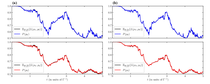
Figure 1: The ensemble average of the linear fidelity between the conditioned state and the true state, and the purity of the conditioned state, for the quantum system of Eq. (9), where Alice and Bob are monitoring the same channel with equal measurement efficiency ($\eta=0.5$) using Y-homodyne detection and photodetection, respectively. To show the convergence of the average linear fidelity to the purity we have computed the averages using a small number of unobserved trajectories and also a larger number. Specifically, in the plots on the left-hand side, the ensemble averages for the smoothed quantum state and the average linear fidelity have been taken over $M=2\times 10^{3}$ and $N=3\times 10^{3}$ unobserved jump trajectories, respectively, while the corresponding figures for the right-hand side are $M=2\times 10^{4}$ and $N=3\times 10^{4}$. Note, the observed record is fixed in all cases and the ensemble of unobserved records used to generate the smoothed state and to average the linear fidelity are generated independently. As we can see, for both the filtered state (top graphs) and the smoothed state (bottom graphs), Eq. (6) holds. Here, $\hbar=1$, $\Omega=3\Gamma$ and $\eta=0.5$.

III Cost Function: Relative Entropy

We now move our attention to another cost function, the relative entropy with the true state. The consideration of this cost function in stems from the work in Ref. García-Pintos and del Campo (2019), where the authors derived bounds on the average relative entropy between the state obtained by an omnicient observer (the true state) and either an ignorant (one who has no measurement information) or partially ignorant (one who has a fraction of the measurement output). The key difference here is that we are considering the optimal estimator that minimizes the (conditional) averarge of the relative entropy, as opposed to finding the upper and lower bounds. Furthermore, we consider a more general setting, allowing the omniscient observer to perform a different measurement (Bob’s measurement in our formulation) on the remaining portion of the output to the partially ignorant observer (Alice in our formulation).

The relative entropy is defined as Vedral (2002); Ruskai (2002); Audenaert (2014)

$$S(\rho||\sigma)=\text{Tr}[\rho\log\rho]-\text{Tr}[\rho\log\sigma]\,.$$ (10)

$S(\rho||\sigma)$ is a measure of state distinguishability between state $\rho$ and $\sigma$, more specifically, it is akin to the likelihood that state $\sigma$ will not be confused with state $\rho$, where a relative entropy of zero corresponds to completely indistinguishable states. Note, unlike a lot of other cost functions, like the TrSD, the relative entropy is not symmetric in its arguments. Consequently, the estimation task is to find the state that minimizes the risk function

$${\cal R}^{\rm RE}_{{\rm O}_{\Xi}}(\check{\rho})=\mathbb{E}_{\overleftarrow{\rm U}|{\rm O}_{\Xi}}\{S(\rho_{\text{T}}||\check{\rho})\}\,.$$ (11)

Once again, the state that minimizes this risk function is the usual conditioned state. We can show the optimality of this state using the same method as before, that is, any state $\rho^{\prime}\neq\rho_{{\rm O}_{\Xi}}$ will be suboptimal. Substituting $\rho^{\prime}$ into the risk function we get

$$\begin{split}{\cal R}^{\rm RE}_{{\rm O}_{\Xi}}(\rho^{\prime})&=\mathbb{E}_{\overleftarrow{\rm U}|{\rm O}_{\Xi}}\{\text{Tr}[\rho_{\text{T}}\log\rho_{\text{T}}]-\text{Tr}[\rho_{\text{T}}\log\rho^{\prime}]\}\\ &=\mathbb{E}_{\overleftarrow{\rm U}|{\rm O}_{\Xi}}\{\text{Tr}[\rho_{\text{T}}\log\rho_{\text{T}}]-\text{Tr}[\rho_{{\rm O}_{\Xi}}\log\rho_{{\rm O}_{\Xi}}]\}\\ &+\mathbb{E}_{\overleftarrow{\rm U}|{\rm O}_{\Xi}}\{\text{Tr}[\rho_{{\rm O}_{\Xi}}\log\rho_{{\rm O}_{\Xi}}]-\text{Tr}[\rho_{\text{T}}\log\rho^{\prime}]\}\,.\end{split}$$ (12)

Remembering that $\rho_{{\rm O}_{\Xi}}=\mathbb{E}_{\overleftarrow{\rm U}|{\rm O}_{\Xi}}\{\rho_{\text{T}}\}$, the risk function becomes

$$\begin{split}{\cal R}_{{\rm O}_{\Xi}}^{\rm RE}(\rho^{\prime})&=\mathbb{E}_{\overleftarrow{\rm U}|{\rm O}_{\Xi}}\{S(\rho_{\text{T}}||\rho_{{\rm O}_{\Xi}})\}+S(\rho_{{\rm O}_{\Xi}}||\rho^{\prime})\\ &>\mathbb{E}_{\overleftarrow{\rm U}|{\rm O}_{\Xi}}\{S(\rho_{\text{T}}||\rho_{{\rm O}_{\Xi}})\}\,,\end{split}$$ (13)

where the inequality results from the fact that the relative entropy is non-negative and is saturated only when $\rho^{\prime}=\rho_{{\rm O}_{\Xi}}$ Ruskai (2002).

In a similar vein to the TrSD case, when we restrict to pure true states, the expected risk function of the conditioned state simplifies to the von Neumann entropy of $\rho_{{\rm O}_{\Xi}}$, that is

$${\cal R}_{{\rm O}_{\Xi}}^{\rm RE}(\rho_{{\rm O}_{\Xi}})=S(\rho_{{\rm O}_{\Xi}})\,.$$ (14)

This follows from the fact that for a pure state $\rho$, $\text{Tr}[\rho\log\rho]=0$. Note, a similar equality was also derived in Ref. García-Pintos and del Campo (2019), however they only considered the average over both the observed and unobserved records and not the conditional averages. We verify that this equality is correct using the the previous physical example in Eq. (9), with good agreement seen in Fig. 2.

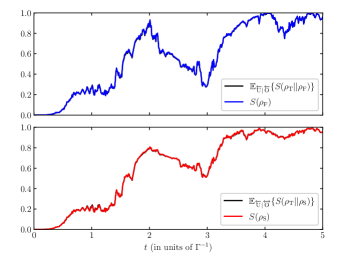
Figure 2: The relative entropy risk function for the filtered state (top) and smoothed state (bottom) for the quantum system described in Eq. (9). We have also computed the von Neumann entropy to illustrate the equality in Eq. (11) holds, using $\log_{2}$ in both cases. Other details, including the randomly generated observed record $\overleftrightarrow{\rm O}$, are as in Fig. 1 (b).

IV Cost Function: Linear Infidelity

Given the previous two cost functions, one might assume that the conditioned state $\rho_{{\rm O}_{\Xi}}$ would be the optimal estimator for any cost function that was a distance/distinguishability measure. However, this is not the case. The last measure we will consider as a cost function is the linear infidelity (LI) with the true state, i.e., ${\cal C}(\check{\rho},\rho_{\text{T}})=1-L(\check{\rho},\rho_{\text{T}})$, where the linear fidelity is defined in Eq. (4). Note, one will obtain the same cost function for the Jozsa infidelity when assuming a pure true state, as discussed above. Once again, the task is to find the state that minimizes the risk function, here

$${\cal R}^{\rm LI}_{{\rm O}_{\Xi}}(\check{\rho})=\mathbb{E}_{\overleftarrow{\rm U}|{\rm O}_{\Xi}}\{1-L(\check{\rho},\rho_{\text{T}})\}\,.$$ (15)

By the linearity of the trace, we can immediately simplify this risk function to ${\cal R}^{\rm LI}_{{\rm O}_{\Xi}}(\check{\rho})=1-\text{Tr}[\check{\rho}\rho_{{\rm O}_{\Xi}}]$. Furthermore, we can reframe the optimization problem in this case to find the estimated state $\check{\rho}$ that maximize the linear fidelity $L(\check{\rho},\rho_{{\rm O}_{\Xi}})=\text{Tr}[\check{\rho}\rho_{{\rm O}_{\Xi}}]$.

Now, using the fact that $\rho_{{\rm O}_{\Xi}}$ is Hermitian and hence diagonalizable with some unitary matrix $U$, the linear fidelity becomes

$$\begin{split}\text{Tr}[\check{\rho}\rho_{{\rm O}_{\Xi}}]=&\text{Tr}[\check{\rho}U\Lambda_{{\rm O}_{\Xi}}U^{\dagger}]=\sum_{i}\lambda_{i}(U^{\dagger}\check{\rho}U)_{ii}\\ =&\lambda_{{\rm O}_{\Xi}}^{\rm max}\sum_{i}\frac{\lambda_{i}}{\lambda_{{\rm O}_{\Xi}}^{\rm max}}(U^{\dagger}\check{\rho}U)_{ii}\,,\end{split}$$ (16)

where $\Lambda_{{\rm O}_{\Xi}}$ is a diagonal matrix whose entries are the eigenvalues $\lambda_{i}$ of $\rho_{{\rm O}_{\Xi}}$ and $\lambda_{{\rm O}_{\Xi}}^{\rm max}$ is the largest eigenvalue of $\rho_{{\rm O}_{\Xi}}$. Since $\rho_{{\rm O}_{\Xi}}$ is positive semidefinite, as it is a valid quantum state, $0\leq\lambda_{i}/\lambda_{{\rm O}_{\Xi}}^{\rm max}\leq 1$. Furthermore, we know $(U^{\dagger}\check{\rho}U)_{ii}$ is positive since $\check{\rho}$ must be a valid quantum state and hence is positive semidefinite. Thus we can take the upper bound on $\lambda_{i}/\lambda_{{\rm O}_{\Xi}}^{\rm max}$, giving an upper bound on the linear infidelity

$$\text{Tr}[\check{\rho}\rho_{{\rm O}_{\Xi}}]\leq\lambda_{{\rm O}_{\Xi}}^{\rm max}\sum_{i}(U^{\dagger}\check{\rho}U)_{ii}=\lambda_{{\rm O}_{\Xi}}^{\rm max}\text{Tr}[U^{\dagger}\check{\rho}U]=\lambda_{{\rm O}_{\Xi}}^{\rm max}\,,$$ (17)

where the final equality is obtained using the cyclic property of the trace and $\text{Tr}[\check{\rho}]=1$. We can saturate the upper bound in Eq. (17) by choosing the estimate state to be

$$\rho_{{\rm O}_{\Xi}}^{\rm L}=|{\psi_{{\rm O}_{\Xi}}^{\rm max}}\rangle\langle{\psi_{{\rm O}_{\Xi}}^{\rm max}}|\,,$$ (18)

$|{\psi_{{\rm O}_{\Xi}}^{\rm max}}\rangle$ is the eigenstate corresponding to the largest eigenvalue $\lambda_{{\rm O}_{\Xi}}^{\rm max}$ of the conditioned state. Since this state estimator is, in some sense, a purification of the conditioned state, we will call this state the lustrated conditioned state, hence the superscript ${\rm L}$.

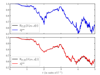
Figure 3: The ensemble average of the linear fidelity between the true state and the lustrated conditioned state and the maximum eigenvalue of the conditioned state for the quantum system in Eq. (9) with Alice and Bob using Y-homodyne detection and photodetection, respectively. Other details, including the randomly generated observed record $\overleftrightarrow{\rm O}$, are as in Fig. 1 (b).

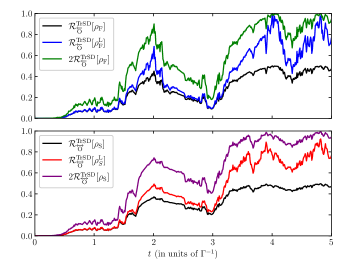
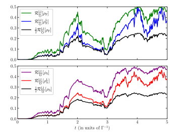
Figure 4: The TrSD (left) and LI (right) risk functions for the lustrated conditioned state for the system in Eq. (9). In both instances, we evaluate the risk function for the lustrated smoothed (top) and the lustrated filtered (bottom) state, where the bounds on the risk functions in terms of the relevant conditioned states are shown in each case, validating the bounds Eq. (22) (left) and Eq. (23) (right). Other details, including the randomly generated observed record $\overleftrightarrow{\rm O}$, are as in Fig. 1 (b).

As was the case for the previous two cost functions, the risk function for the optimal estimator can be simplified to

$${\cal R}^{\rm LI}_{{\rm O}_{\Xi}}[\rho_{{\rm O}_{\Xi}}^{\rm L}]=1-\lambda_{{\rm O}_{\Xi}}^{\rm max}\,,$$ (19)

which follows trivially from

$${\mathbb{E}}_{\overleftarrow{\rm U}|{\rm O}_{\Xi}}\{L(\rho_{{\rm O}_{\Xi}}^{\rm L},\rho_{\text{T}})\}=\lambda_{{\rm O}_{\Xi}}^{\rm max}$$ (20)

In this case, contrary to the other distance measures, we notice that the risk function does not reduce to a simple measure of the optimal estimator. Instead the risk function depends on the conditioned state. To verify Eq. (20), we will consider the (not-lustrated) physical system presented in Sec. II. In Fig. 3, we indeed see that the average fidelity of the lustrated conditioned state $\rho_{{\rm O}_{\Xi}}^{\rm L}$ is equal to the largest eigenvalue of the conditioned state $\rho_{{\rm O}_{\Xi}}$.

Due to the similarity between the LI and the TrSD cost functions, it is possible to derive upper and lower bounds on the risk function of the lustrated state for both a LI and a TrSD cost. To begin, since the lustrated conditioned state is the optimal estimator for the LI risk function, we have the trivial bound

$${\cal R}^{\rm LI}_{{\rm O}_{\Xi}}[\rho_{{\rm O}_{\Xi}}^{\rm L}]\leq{\cal R}^{\rm LI}_{{\rm O}_{\Xi}}[\rho_{{\rm O}_{\Xi}}]\,,$$ (21)

where an equality occurs when the conditioned state is pure. Whilst this is trivial for a LI cost, this relationship places a non-trivial upper bound on the TrSD risk function for the lustrated conditioned state. Specifically, it is easy to show, using Eq. (6) and assuming a pure true state, that Eq. (21) implies that ${\cal R}^{\rm TrSD}_{{\rm O}_{\Xi}}[\rho_{{\rm O}_{\Xi}}^{\rm L}]\leq 2{\cal R}^{\rm TrSD}_{{\rm O}_{\Xi}}[\rho_{{\rm O}_{\Xi}}]$. Similarly, we can derive a lower bound on the LI risk function for the lustrated conditioned state by considering ${\cal R}^{\rm TrSD}_{{\rm O}_{\Xi}}[\rho_{{\rm O}_{\Xi}}]\leq{\cal R}^{\rm TrSD}_{{\rm O}_{\Xi}}[\rho_{{\rm O}_{\Xi}}^{\rm L}]$. In this case, we obtain the lower bound $\mbox{$\frac{1}{2}$}{\cal R}^{\rm LI}_{{\rm O}_{\Xi}}[\rho_{{\rm O}_{\Xi}}]\leq{\cal R}^{\rm LI}_{{\rm O}_{\Xi}}[\rho_{{\rm O}_{\Xi}}^{\rm L}]$. As a result, we obtain the following bounds for the on the risk functions of the lustrated conditioned state

$${\cal R}^{\rm TrSD}_{{\rm O}_{\Xi}}[\rho_{{\rm O}_{\Xi}}]\leq{\cal R}^{\rm TrSD}_{{\rm O}_{\Xi}}[\rho_{{\rm O}_{\Xi}}^{\rm L}]\leq 2{\cal R}^{\rm TrSD}_{{\rm O}_{\Xi}}[\rho_{{\rm O}_{\Xi}}]\,.$$ (22)

$$\mbox{$\frac{1}{2}$}{\cal R}^{\rm LI}_{{\rm O}_{\Xi}}[\rho_{{\rm O}_{\Xi}}]\leq{\cal R}^{\rm LI}_{{\rm O}_{\Xi}}[\rho_{{\rm O}_{\Xi}}^{\rm L}]\leq{\cal R}^{\rm LI}_{{\rm O}_{\Xi}}[\rho_{{\rm O}_{\Xi}}]\,,$$ (23)

To verify these bounds on the risk functions, we will once again consider the physical example presented in Sec. II. In Fig. 4, we consider the both TrSD (left) and LI (right) risk functions for the smoothed (top) and filtered (bottom) state, observing the bounds in Eqs. (23)–(22). Note, one might think that the upper bound in Eq. (22) could become a trivial bound when ${\cal R}^{\rm TrSD}_{{\rm O}_{\Xi}}[\rho_{{\rm O}_{\Xi}}]>1$ as the maximum value of the TrSD risk function is $2$. In fact, this is never trivial as, from Eq. (7), we can see that ${\cal R}^{\rm TrSD}_{{\rm O}_{\Xi}}[\rho_{{\rm O}_{\Xi}}]\leq 1$.

V Conclusion

In this paper, we have shown that the smoothed quantum state is an optimal state estimator. Specifically, the smoothed quantum state simultaneously minimizes the risk function for a trace-square deviation and relative entropy cost function. Furthermore, we showed that, in both cases, the risk function of the smoothed state reduced to simple measures acting the solely on the smoothed state, specifically, the impurity and von Neumann entropy of the smoothed state, respectively. However, when we considered the linear infidelity as a cost function we found, somewhat counter-intuitively, that the smoothed quantum state was not optimal. Instead, the the lustrated smoothed state, defined as the eigenstate corresponding to the maximum eigenvalue of the smoothed quantum state, is the optimal estimator for such a cost function.

As was the case for the other cost functions, we showed that the linear infidelity risk function of the lustrated smoothed state reduces to a simple measure. However, in this case the measure does not depend on the lustrated smoothed state itself, rather it depends on the maximum eigenvalue of the smoothed quantum state. Finally, we calculated some upper and lower bounds on the the risk function of the lustrated smoothed state, for both the trace-square deviation and the linear infidelity.

Since the lustrated state is pure, an obvious question is whether it is related to the pure states in the most likely paths approach of Refs. Chantasri et al. (2013); Weber et al. (2014). This, and many other related questions, are answered by the general cost function approach to quantum state estimation using past and future measurement records introduced in Ref. Chantasri et al. (2021). However, the most-likely path Chantasri et al. (2013); Weber et al. (2014); Chantasri et al. (2021) is restricted to homodyne-like unknown records, whereas in this paper we have used an example here the unknown record is comprised of discrete photon counts. It remains an open question as to whether the most-likely path cost functions of Ref. Chantasri et al. (2021) can be generalized to such cases.

Appendix A Numerics

In this appendix, we present the methods used to compute the filtered, true and smoothed quantum states and all the measures in this paper. To begin, a typical homodyne measurement current, which will remain fixed for all calculations, was generated in with parallel the associated filtered state and calculating the measurement current via

$${\rm d}J_{\phi}(t)=\text{Tr}[\hat{c}_{\phi}\rho_{\text{F}}(t)+\rho_{\text{F}}(t)\hat{c}_{\phi}^{\dagger}]+{\rm d}W_{\text{F}}(t)\,,$$ (24)

where ${\rm d}W_{\text{F}}$ is the filtered innovation generated from a Gaussian distribution with the moments in Eq. (8). The filtered state was computed using quantum maps Wiseman and Milburn (2010), where the evolution of the filtered state in a finite time step $\delta t$ is given by

$$\rho_{\text{F}}(t+\delta t)=\frac{{\cal M}_{H}{\cal M}_{{\rm d}J_{\phi}(t)}{\cal M}_{u}\rho_{\text{F}}(t)}{\text{Tr}[{\cal M}_{H}{\cal M}_{{\rm d}J_{\phi}(t)}{\cal M}_{u}\rho_{\text{F}}(t)]}\,,$$ (25)

where the completely positive map ${\cal M}_{A}$ subscripts denote the particular type of evolution the system is undergoing: $\hat{H}$ denotes the Hamiltonian part, ${\rm d}J_{\phi}(t)$ denotes the homodyne part and $u$ denotes the remaining unconditioned dynamics. The Hamiltonian part is ${\cal M}_{H}\bullet={\rm exp}(-iH\delta t)\bullet{\rm exp}(iH\delta t)$. The unconditioned map can be described by averaging over Bob’s jump process to make a trace-preserving map,

$${\cal M}_{u}\bullet=\sum_{{\rm d}N(t)=0}^{1}\hat{M}_{{\rm d}N(t)}\bullet\hat{M}_{{\rm d}N(t)}^{\dagger}\,.$$ (26)

The homodyne (conditioned) map is described by a single measurement operator ${\cal M}_{{\rm d}J_{\phi}(t)}\bullet=\hat{M}_{{\rm d}J_{\phi}(t)}\bullet\hat{M}_{{\rm d}J_{\phi}(t)}^{\dagger}$. In particular, we used completely positive quantum maps Guevara and Wiseman (2020), where the $\hat{M}$ operators have been taken to a second order in $\delta t$ to ensure the positivity of the quantum state to high accuracy. For details on the particular operators used for the homodyne measurement and the jump measurement see Ref. Guevara and Wiseman (2020).

With this typical record, both the unnormalized filtered state $\tilde{\rho}_{\text{F}}$ and the unnormalized true state $\tilde{\rho}_{\text{T}}$ can be computed. The unnormalized filtered state is computed using Eq. (25) without the trace term on the denominator, and the unnormalized true state evolves as

$$\tilde{\rho}_{\text{T}}(t+\delta t)={\cal M}_{H}{\cal M}_{{\rm d}J_{\phi}(t)}{\cal M}_{{\rm d}N(t)}\rho_{\text{T}}(t)\,.$$ (27)

The reason why the unnormalized versions of these states are computed, as opposed to the normalized version, is is because their traces correspond to the ostensible probability distributions $\text{Tr}[\tilde{\rho}_{\text{F}}]=\wp_{\rm ost}(\overleftarrow{\rm O})$ and $\text{Tr}[\tilde{\rho}_{\text{T}}]=\wp_{\rm ost}(\overleftarrow{\rm O},\overleftarrow{\rm U})$. These distributions are needed for computing the ensemble average over $\overleftarrow{\rm U}$ given $\overleftarrow{\rm O}$ via $\wp_{\rm ost}(\overleftarrow{\rm U}|\overleftarrow{\rm O})=\wp_{\rm ost}(\overleftarrow{\rm O},\overleftarrow{\rm U})/\wp_{\rm ost}(\overleftarrow{\rm O})$. Specifically, the ensemble average using this conditional probability is

$$\mathbb{E}_{\overleftarrow{\rm U}|\overleftarrow{\rm O}}\{\bullet\}=\frac{1}{N_{\rm tot}}\sum_{n=1}^{N_{\rm tot}}\frac{\text{Tr}[\tilde{\rho}_{\text{T}}^{(n)}]}{\text{Tr}[\tilde{\rho}_{\text{F}}]}\bullet\,,$$ (28)

where the superscript $(n)$ labels the $n$th realization of the true state with $N_{\rm tot}$ being the total number of realizations computed.

For the smoothed quantum state, it is necessary to perform the ensemble average $\mathbb{E}_{\overleftarrow{\rm U}|\overleftrightarrow{\rm O}}$. Thus we require the ostensible distribution $\wp_{\rm ost}(\overleftarrow{\rm U}|\overleftrightarrow{\rm O})=\wp_{\rm ost}(\overleftrightarrow{\rm O},\overleftarrow{\rm U})/\wp_{\rm ost}(\overleftrightarrow{\rm O})$. Both the numerator and denominator are obtained by introducing the retrofiltered effect $\hat{E}_{\text{R}}$, a POVM element that evolve backwards-in-time from a final uninformative state $\hat{E}_{\text{R}}(T)=I$ conditioning on the measurement result back to the time $\tau$. The retrofiltered effect is computed as the adjoint of the unnormalized filtered state, that is,

$$\hat{E}_{\text{R}}(t-\delta t)={\cal M}_{u}^{\dagger}{\cal M}_{{\rm d}J_{\phi}(t)}^{\dagger}{\cal M}_{H}^{\dagger}\hat{E}_{\text{R}}(t)\,,$$ (29)

where $\text{Tr}[\hat{E}_{\text{R}}\rho]=\wp(\overrightarrow{\rm O}|\rho)$. The ostensible distributions are then obtain by $\text{Tr}[\tilde{\rho}_{\text{T}}\hat{E}_{\text{R}}]=\wp_{\rm ost}(\overleftrightarrow{\rm O},\overleftarrow{\rm U})$ and $\text{Tr}[\tilde{\rho}_{\text{F}}\hat{E}_{\text{R}}]=\wp_{\rm ost}(\overleftrightarrow{\rm O})$. Thus the ensemble average conditioning on $\overleftrightarrow{\rm O}$ is computed as

$$\mathbb{E}_{\overleftarrow{\rm U}|\overleftrightarrow{\rm O}}\{\bullet\}=\frac{1}{N_{\rm tot}}\sum_{n=1}^{N_{\rm tot}}\frac{\text{Tr}[\tilde{\rho}_{\text{T}}^{(n)}\hat{E}_{\text{R}}]}{\text{Tr}[\tilde{\rho}_{\text{F}}\hat{E}_{\text{R}}]}\bullet\,.$$ (30)

Note, for a fair comparison of the various equalities presented in this paper, the ensemble of true states (of size $M$) used to compute the ensemble average for the smoothed state were generated independently of the ensemble of true states (of size $N$) used to compute the ensemble averages of other quantities, like the linear fidelities and relative entropies.

References

- Belavkin (1987) V. P. Belavkin, Information, complexity and control in quantum physics, edited by A. Blaquíere, S. Dinar, and G. Lochak (Springer, New York, 1987).
- Belavkin (1992) V. P. Belavkin, Commun. Math. Phys. 146, 611 (1992).
- Wiseman and Milburn (2010) H. M. Wiseman and G. J. Milburn, Quantum Measurement and Control (Cambridge University Press, Cambridge, England, 2010).
- Weinert (2001) H. L. Weinert, Fixed Interval Smoothing for State Space Models (Kluwer Academic, New York, 2001).
- Haykin (2001) S. Haykin, Kalman Filtering and Neural Networks (Wiley, New York, 2001).
- Trees and Bell (2013) H. L. V. Trees and K. L. Bell, Detection, Estimation, and Modulation Theory, Part I: Detection, Estimation, and Filtering Theory, 2nd ed. (John Wiley and Sons, New York, 2013).
- Brown and Hwang (2012) R. G. Brown and P. Y. C. Hwang, Introduction to Random Signals and Applied Kalman Filtering, 4th ed. (Wiley, New York, 2012).
- Einicke (2012) G. A. Einicke, Smoothing, filtering and prediction: Estimating the past, present and future (InTech Rijeka, 2012).
- Friedland (2012) B. Friedland, Control system design: an introduction to state-space methods (Courier Corporation, 2012).
- Särkkä (2013) S. Särkkä, Bayesian filtering and smoothing, Vol. 3 (Cambridge University Press, 2013).
- Aharonov et al. (1964) Y. Aharonov, P. G. Bergmann, and J. L. Lebowitz, Phys. Rev. 134, B1410 (1964).
- Aharonov et al. (1988) Y. Aharonov, D. Z. Albert, and L. Vaidman, Phys. Rev. Lett. 60, 1351 (1988).
- Tsang (2009a) M. Tsang, Phys. Rev. Lett. 102, 250403 (2009a).
- Tsang (2009b) M. Tsang, Phys. Rev. A 80, 033840 (2009b).
- Chantasri et al. (2013) A. Chantasri, J. Dressel, and A. N. Jordan, Phys. Rev. A 88, 042110 (2013).
- Gammelmark et al. (2013) S. Gammelmark, B. Julsgaard, and K. Mølmer, Phys. Rev. Lett. 111, 160401 (2013).
- Guevara and Wiseman (2015) I. Guevara and H. Wiseman, Phys. Rev. Lett. 115, 180407 (2015).
- Ohki (2015) K. Ohki, in 2015 54th IEEE Conference on Decision and Control (CDC) (2015) pp. 4350–4355.
- Ohki (2019) K. Ohki, in Proceedings of the ISCIE International Symposium on Stochastic Systems Theory and its Applications, Vol. 2019 (The ISCIE Symposium on Stochastic Systems Theory and Its Applications, 2019) pp. 25–28.
- Tsang (2019) M. Tsang, “Quantum analogs of the conditional expectation for retrodiction and smoothing: a unified view,” (2019), arXiv:1912.02711 [quant-ph] .
- Laverick et al. (2019) K. T. Laverick, A. Chantasri, and H. M. Wiseman, Phys. Rev. Lett. 122, 190402 (2019).
- Chantasri et al. (2019) A. Chantasri, I. Guevara, and H. M. Wiseman, New J. Phys. 21, 083039 (2019).
- Laverick et al. (2021a) K. T. Laverick, A. Chantasri, and H. M. Wiseman, Phys. Rev. A 103, 012213 (2021a).
- Laverick et al. (2021b) K. T. Laverick, A. Chantasri, and H. M. Wiseman, Quantum Stud.: Math. Found. 8, 37 (2021b).
- Laverick (2020) K. T. Laverick, (2020).
- Audenaert (2014) K. M. R. Audenaert, Quantum Info. Comput. 14, 31–38 (2014).
- Jozsa (1994) R. Jozsa, J. Mod. Opt. 41, 2315 (1994).
- Vedral (2002) V. Vedral, Rev. Mod. Phys. 74, 197 (2002).
- Ruskai (2002) M. B. Ruskai, J. Math. Phys. 43, 4358 (2002).
- García-Pintos and del Campo (2019) L. P. García-Pintos and A. del Campo, arXiv preprint arXiv:1907.12574 (2019).
- Weber et al. (2014) S. J. Weber, A. Chantasri, J. Dressel, A. N. Jordan, K. W. Murch, and I. Siddiqi, Nature 511, 570 (2014).
- Chantasri et al. (2021) A. Chantasri, I. Guevara, K. T. Laverick, and H. M. Wiseman, (2021), arXiv:2104.02911 [quant-ph] .
- Guevara and Wiseman (2020) I. Guevara and H. M. Wiseman, Phys. Rev. A 102, 052217 (2020).