COLD: Concurrent Loads Disaggregator
for Non-Intrusive Load Monitoring

Abstract

The modern artificial intelligence techniques show the outstanding performances in the field of Non-Intrusive Load Monitoring (NILM). However, the problem related to the identification of a large number of appliances working simultaneously is underestimated. One of the reasons is the absence of a specific data. In this research we propose the Synthesizer of Normalized Signatures (SNS) algorithm to simulate the aggregated consumption with up to 10 concurrent loads. The results show that the synthetic data provides the models with at least as a powerful identification accuracy as the real-world measurements. We have developed the neural architecture named Concurrent Loads Disaggregator (COLD) which is relatively simple and easy to understand in comparison to the previous approaches. Our model allows identifying from 1 to 10 appliances working simultaneously with mean F1-score 78.95%. The source code of the experiments performed is available at https://github.com/arx7ti/cold-nilm.

I Introduction

The Non-Intrusive Load Monitoring (NILM) was proposed by G. Hart in 1992 to estimate the individual loads from the total load (Fig. 1) by analysis of current and voltage waveforms [1]. The NILM is based on analysis of non-intrusive signatures, they can be formally divided into two groups: waveforms with high sampling rate (steady-state, transients) and waveforms with low sampling rate (root-mean-squared values (RMS) over time). Steady-state and transient waveforms can give an information about electronic nature (possible harmonics composition due to non-linearity of a circuit) and state changes. In the latter case the electronic nature is not observable, only the state of an appliance and human usage factor prevail. Formally, signatures related to the RMS values are a particular case of the signatures sampled under high frequency.

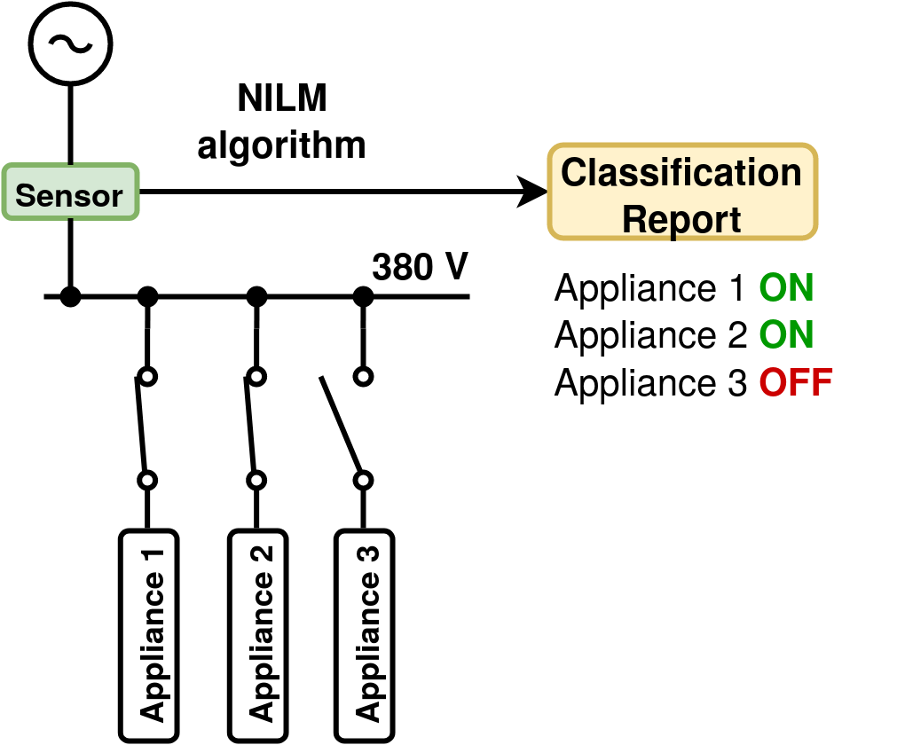
Figure 1: Simplified diagram of the NILM application. Case for 3 different appliances connected to the same bus supplied by the single voltage source

I-A Application

The goal of the NILM is to get an information about individual appliances from their aggregated consumption signal. In its turn, the total consumption signal can be measured by a single meter. The lack of equipment required decreases costs and simplifies the maintenance in residential and industrial use. The formation of the Energy Data Sharing Platform (EDSP) is one of the most promising applications of the NILM [2]. Undoubtedly, the high quality data of energy consumption may improve the electric load forecasting accuracy, therefore load modeling on the generation level may also be precised. The per-device measurements are redundant for utility companies, but this data can be summarized over all the appliances by categories (different types of electronic devices, lighting systems, heating devices, electric motors and etc.). The latter forms a more accurate basis for developing prediction models rather than existing technologies on gathering such kind of a data. This platform may also be helpful for both government and industry in order to perform energy efficient policy (for example, power quality control).

I-B General formulation

The general NILM problem can be formulated as follows. Suppose $L=\{l_{1},l_{2},\ldots,l_{n}\}$ is a set of labels (e.g. $l_{1}="kettle"$). According to the Kirchoff’s Current Law the total consumption signal $c_{\Sigma}\in C_{\Sigma}$ is a sum of continuous functions over time $t$:

$$c_{\Sigma}(t)=\sum_{l\in L}c_{l}(t),$$

where $c_{l}\in C_{l}$ is a signature of a particular appliance $l$. Therefore, the NILM algorithm $N$ is a continuous map which takes a set of aggregated signals and outputs disjoint set of individual signals:

$$N:C_{\Sigma}\rightarrow\bigsqcup_{l\in L}C_{l}.$$

This formulation of the NILM algorithm relates to a combination of regression and classification problems as the output values both labels and corresponding signatures. The supervised learning concept is on the spotlight among NILM researchers [3, 4, 5, 6]. Meaning, in order to reconstruct $N$ the examples of $C_{\Sigma}$ and corresponding $C_{l}$ are needed. Some examples of algorithms of this type are Hidden Markov models, decision trees, neural networks etc.

I-C Features extraction

Nowadays, there is no consensus which time-scale of $C_{\Sigma}$ (and $C_{l}$) (i.e. instantaneous or RMS values) is more beneficial for the NILM algorithm. The models based on the analysis of RMS values show similar results in load identification [7, 8, 9] to the models which take waveforms sampled under high frequency [10, 11]. The choice is more related to the availability of a data and the scale of the NILM problem that the researchers are seeking to solve (real-time or per minute disaggregation). The accuracy of the reconstructing algorithm strictly depends on quality of features extracted from these signatures.

The features may be estimated manually: papers [12, 13] propose different methods for feature extraction from RMS valued real power time sequences. They are median filters, mean values, standard deviation and other numerical metrics. The authors of [14] studied Short-Term Fourier Transform as a feature extractor for signals sampled under high-frequency. Moreover, for the latter signatures the time-domain features as central moments, form factor and temporal centroids can be also beneficial [15]. The manual features extraction from high-frequency measurements provides up to $99\%$ classification accuracy for appliances working stand-alone via KNN or SVM [15, 16, 17]. On the other hand, the deep neural networks can be applied to extract features directly from raw RMS or transient/steady-state waveforms. To date, the research papers [7, 8, 9] propose neural network architectures providing the state of the art accuracy in NILM tasks. These architectures are modifications of convolutional neural networks (CNN) and recurrent neural networks (RNN).

I-D Current limitation

The important thing in the NILM is the disaggregation ability of a model. By this we mean how effective a model can distinguish a number of simultaneously working appliances from each other. Surprisingly, this issue is not paid a much attention to. Most of the papers propose the models which are trained on examples from public-available datasets such as UK-DALE [18], REDD [19], PLAID [20], WHITED [21] etc. Table I shows the summary of these datasets. The instances of the WHITED dataset are individual measurements of each appliance, while the PLAID dataset comprises also aggregated measurements. The recent paper on load disaggregation showed that the maximum number of concurrent loads in the PLAID dataset is 3 [11]. Moreover, we revealed statistics on number of simultaneously working appliances for two most popular NILM datasets: the UK-DALE and REDD. Both datasets are similar in the terms of the structure: measurements are collected from different households and stored separately. Each house contains the list of devices, corresponding the list of power measurements and the list with aggregated power measurements.

TABLE I: Summary of public-available NILM datasets

Dataset	Resolution	# Labels
Plaid (US)	30 kHz	16
REDD (US)	16.5 kHz, 1 Hz	20
UK-DALE (UK)	16 kHz, 1 Hz	40
WHITED (EU,US)	41 kHz	55

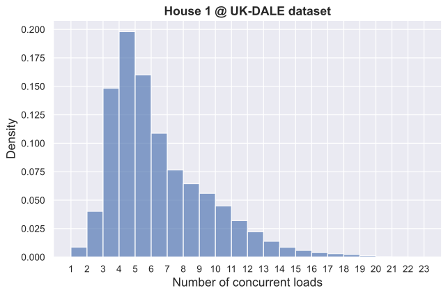
Figure 2: Number of simultaneously working appliances over all measurements from 1st house of the UK-DALE dataset

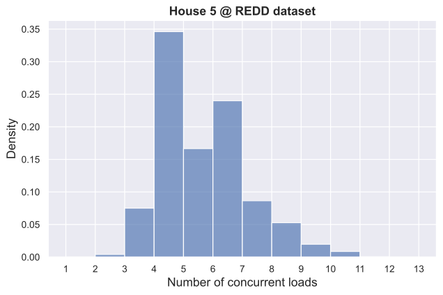
Figure 3: Number of simultaneously working appliances over all measurements from 5th house of the REDD dataset

Fig. 2 and Fig. 3 show how frequently (number of seconds from maximum observable duration of measurements) a particular number of simultaneously working loads appears within UK-DALE’s 1st house and REDD’s 5th house (these houses were taken since they have the largest number of appliances available) correspondingly. The absence of loads is excluded from time scope. Tables II and III represent these distributions for each house of the datasets. Despite dozens of appliances presented in these two datasets, most of the researchers [22, 23, 7, 9] usually select 4-6 appliances from the UK-DALE or REDD datasets for their studies. The author of the UK-DALE dataset in his paper “Deep Neural Networks Applied to Energy Disaggregation” [22] explains his choice of 5 appliances (fridge, washing machine, dish washer, kettle and microwave) as most of these devices appear within 3 houses, that is the training and testing procedures will be consistent; moreover, these appliances take significant share of total consumption and their consumption patterns are heterogeneous [22]. We also studied how frequent the chosen appliances work concurrently: for example, in the 1st house of the UK-DALE dataset the 92.06% of time these 5 appliances are working individually, the rest 7.58% and 0.36% splitted across combinations from 2 to 3 and more respectively. In its turn, this explains significant accuracy ($>$90%) of the models proposed by the authors. Thus, it follows that the issue on disaggregation of larger number of concurrent loads (4 and more) is still open. Similar statistics for the REDD dataset and the rest of the UK-DALE dataset can be found in our repository. Note, that the authors of the UK-DALE and REDD datasets do not group the appliances into major categories (e.g. laptops), they store them separately (e.g. laptop1, laptop2 etc.). Therefore, based on statistics we revealed the two and more concurrent appliances might be from the same category. However, in our approach we will focus only on single appliance from a particular category. For example, we will not consider two different laptops working at the same time.

TABLE II: Distribution of number of concurrent loads in % of time for the UK-DALE dataset

House	1, %	2-5, %	6-9, %	$\geq$10, %	max
1	0.88	54.66	30.58	13.88	23
2	0.00	74.36	25.53	0.10	11
3	93.66	6.34	0.00	0.00	3
4	0.60	99.40	0.00	0.00	5
5	11.90	40.15	46.81	1.13	13

TABLE III: Distribution of number of concurrent loads in % of time for the REDD dataset

House	1, %	2-5, %	6-9, %	$>$10, %	max
1	0.00	85.38	14.16	0.46	13
2	0.41	99.52	0.07	0.00	7
3	21.10	71.90	6.98	0.01	12
4	0.08	97.65	2.27	0.00	11
5	0.01	59.18	39.90	0.91	13
6	0.30	93.17	6.51	0.01	12

I-E Contribution

To resolve the issue on disaggregation of a large number of concurrent loads we propose the Synthesizer of Normalized Signatures (SNS) which takes measurement data from different NILM datasets of high sampling rate signatures, normalizes them and produces an aggregated signal (total load) for each random combination of appliances. In this case the goal is to synthesize well-balanced dataset enough to train the models for suitable multi-label classification results at different number of concurrent loads. We used the PLAID and WHITED datasets as reference datasets due to the hypothesis that signatures sampled under high-frequency have maximum information content unlike RMS values [24].

Besides SNS algorithm, we propose the neural network architecture named COLD (Concurrent Loads Disaggregator) that is based on deep ReLU network [25] and multi-head self attention mechanism [26]. The network takes spectrograms of 5 seconds-long aggregated signals as input data and outputs categories of appliances being detected within such period of time. The model was evaluated across 1 to 10 simultaneously working appliances from 55 different categories.

This paper is organized as follows: the Section II is devoted to the Synthesizer of Normalized Signatures algorithm with implementation details. The Section III of the paper describes the contemporary methods of the neural networks theory, the COLD architecture proposed. The Section IV explains the input data format, loss function and evaluation metric. The Section V presents the results of the hyperparameters search procedure and the model evaluation. In the Section VI the comparison of our results with the previous state-of-the-art NILM models is given. Finally, the Section VII summarizes the attempts to solve the problem and proposes our research prospects.

II Synthesizer of Normalized Signatures (SNS)

The datasets discussed before might contain dozens of concurrent loads. However, our statistics show that 10 and more appliances work simultaneously very rarely. Unlike residential sector the number of concurrent appliances in offices or in another non-residential spaces can be much higher. Therefore, more additional data is required. Traditional data collection process (measurement of real electric lifecycle) is time-expensive and produces a lot of useless measurements (e.g. zero consumption). To address this issue the synthetic data based on real signatures of devices can be used. That is the one can only measure current and voltage consumption patterns (sampled under high rate in our case) by particular device under different states (switch on/off, mode change etc). Then, these measurements can be combined with accordance to circuits laws to simulate aggregated consumption. Thus, the time of measurements reduces significantly. As it will be shown in Section VI the results of disaggregation on synthetic data at least as powerful as real-life data.

To synthesize the new dataset out of independent measurements of appliances the SNS algorithm is introduced. We used only WHITED and PLAID datasets as reference since only they were available at this time. Both datasets comprise 55 and 16 categories of devices with 1343 and 1876 available individual measurements (1 recording per 1 running device) respectively. Each category contains current and voltage signatures for either different devices of the same type or same device of different states. Both datasets have 15 common categories: soldering iron, fridge, laptop, washing machine, hairdryer, light bulb, heater, fan, cfl, coffee machine, kettle, flatiron, microwave, vacuum cleaner and air conditioner. There is no doubt, that the concatenation of these classes can increase heterogeneity as two datasets were obtained independently in different power grids.

II-A Signatures normalization

At the first step the SNS algorithm reads and standartizes signatures in 6 steps:

1. Voltage quality control - instance with total harmonic distortion of voltage exceeding threshold $t_{THD}$ are dropped from the scope.

2. Region of interest extraction - root-mean-square (RMS) values over entire current waveform are calculated from sliding window of one-period size. Then, binary mask is applied under condition of RMS values being above activation threshold $t_{on}$.

3. Signal duration control - signature of duration less than $t_{sec}$ seconds is dropped, otherwise duration is rounded to an integer value to avoid spectral-leakage for further procedures;

4. Frequency normalization - both voltage and current waveforms are transformed to reference frequency $f_{ref}$ with time-stretch method proposed by librosa library [27]. Waveforms are stretched in $f_{0}/f_{ref}$ times ($f_{0}$ is actual fundamental frequency) to avoid fluctuations and to match signatures from different-frequency power grids (e.g. US and EU);

5. Downsampling - the original waveforms are resampled to $f_{down}$ to reduce the memory usage without significant loss of information;

6. Scaling - the voltage waveform is scaled to reference voltage $v_{ref}$. The current waveform is also rescaled to preserve power consumption.

Accepted signatures (patterns) are combined in a common baseline dataset $P$.

II-B Distribution of concurrently working appliances

Subset $L_{w}\subset L$ comprises $w=|L_{w}|$ ($1\leq w\leq|L|$) labels of appliances appeared within an observation interval of duration $T_{obs}$. To build a synthetic collection $S_{w}$ different combinations of labels are used, where each label has some probability to be selected i.e. $L_{w}\sim\Pr(L)$. In this work, we set $\Pr(L)=\mathcal{U}(1,|L|)$ to achieve label-balanced distribution. Therefore, for each $w$ there is a bound on number of such combinations: $b_{comb}(w)=\binom{|L|}{w}$. However, for some cases $b_{comb}(w)$ can be prohibitively big number. Thus, a limit $\hat{b}_{comb}(w)$ was introduced, s.t. actual number of combinations to be selected is defined as $\min(b_{comb}(w),\hat{b}_{comb}(w))$.

Let $P_{l}\in P$ be the patterns that corresponds to a particular label $l\in L$, then for each label $l$ there is $|P_{l}|\geq 1$. This makes possible to represent each combination in following number of ways: $b_{repr}=\prod_{l\in L_{w}}|P_{l}|$. Another penalization on number of such representations is $\hat{b}_{repr}$. To determine how many times some combination of labels $L_{w}$ can be repeated the following weight is introduced:

$$\Omega=\frac{\prod_{l\in L_{w}}p(l)\in\Pr(L)}{\sum_{l\in L}p(l)\in\Pr(L)}$$

Thus, the $\min(\Omega\cdot b_{repr}(w),\hat{b}_{repr}(w))$ corresponds to the number of unique aggregated signals obtained from single $L_{w}$.

II-C Summation of signals

Once combinations $L_{w}$ and their representations are given, the start time of appliance from representation can be taken at random. It can be also taken as a point before observation, but with the restriction on signature not to be ended in the very beginning of observation period and not to be started in the very end.

At the final step the algorithm loops over each representation of each combination $L_{w}$ and does phase alignment with following point-wise summation. Here for each representation of $L_{w}$ one of the corresponding voltage waveform is taken arbitrary as reference, while the others are being shifted until their peaks are aligned. Then the current waveforms are aligned by shifts obtained at previous step. This procedure is needed due to the natural requirement for given appliances being supplied by the same voltage source.

Thus, the algorithm can be defined as $SNS:P\rightarrow S_{w}$, where $S_{w}$ is a synthetic collection of aggregated signatures for particular $w$. The entire synthetic dataset can be written in the form:

$$S=\bigcup_{w=1}^{w_{max}}S_{w},$$

II-D Proposed settings

We set following parameters for the signatures normalization step: $t_{THD}=0.1$, $t_{on}=0.1\ A$, $t_{sec}=1\ s$, $f_{ref}=50.0\ Hz$, $f_{down}=4000\ Hz$, $v_{ref}=311\ V$. After running this step under given parameters 4 signatures of the WHITED and 208 signatures of the PLAID were dropped. Most of these patterns were related to the category “blender”, as the result this category of appliances became empty and was also dropped from the scope. The cardinality of dataset $P$ is 3007. Later on, each category of $P$ was randomly shuffled and splitted into 3 subsets by portions 60%, 10%, 30%. Therefore, the new datasets were obtained: $P_{train}$, $P_{val}$ and $P_{test}$ for training, validating and testing procedures respectively. The idea here is to get rid of leakage of unique signatures between these datasets.

At the second step, parameters of the distributions of simultaneously working devices need to be defined to synthesize well-balanced datasets $S_{train}$, $S_{val}$ and $S_{test}$. At first, we set $T_{obs}=5$ seconds, meaning that the SNS will produce 5 seconds-long waveforms of aggregated loads. Then, we set bounds on combinations $\hat{b}_{comb}$ and representations $\hat{b}_{repr}$ for each case of $w=2\dots 10$. The special case is $w=1$ where the signatures of $P$ are randomly shifted over the time interval. There is no instructions on how to set bounds properly, thus, we propose an intuitive approach:

1. increase number of representations $\hat{b}_{repr}$ of each combination for smaller $w$ to estimate individual signatures more precisely;

2. decrease number of representations for higher $w$ and increase number of combinations $\hat{b}_{comb}$ to improve disaggregation ability.

To estimate density of signatures per combination we computed median values from cardinalities of each category for corresponding patterns $P_{train}$, $P_{val}$, $P_{test}$. Median values were used as initial for $w=2$ to set the density $\frac{\hat{b}_{repr}}{\hat{b}_{comb}}$, then with growing $w$ this ratio was decreasing by factor of 2. It is assumed that the model should be able to disaggregate the signal not to memorize the combinations of loads, therefore, collections for $w=\{1,2,5,7,9\}$ were skipped in case of training dataset to avoid the overfitting of a model (Table IV). As for validating and testing collections the values $w=\{1,2,5,7,9\}$ are included (Tables V, VI). Finally, the SNS produced following synthetic datasets $S_{train}$, $S_{val}$ and $S_{test}$ with cardinalities 120000, 36295 and 108912 respectively. Some examples were cut by $b_{repr}$ during the generation process.

TABLE IV: Parameters for distribution of simultaneously working loads. Case for training dataset

w	$\hat{b}_{comb}$	$\hat{b}_{repr}$	reprs/comb
3	1000	12000	12
4	1000	12000	12
6	2000	12000	6
8	4000	12000	3
10	4000	12000	3

TABLE V: Parameters for distribution of simultaneously working loads. Case for validating dataset

w	$\hat{b}_{comb}$	$\hat{b}_{repr}$	reprs/comb
1	55	-	-
2	500	1000	2
3	500	1000	2
4	500	1000	2
5	1000	1000	1
6	1000	1000	1
7	1000	1000	1
8	2000	2000	1
9	2000	2000	1
10	2000	2000	1

TABLE VI: Parameters for distribution of simultaneously working loads. Case for testing dataset

w	$\hat{b}_{comb}$	$\hat{b}_{repr}$	reprs/comb
1	55	-	-
2	500	3000	6
3	500	3000	6
4	500	3000	6
5	1000	3000	3
6	1000	3000	3
7	1000	3000	3
8	2000	2000	1
9	2000	2000	1
10	2000	2000	1

III Model Description

The choice of the neural network architecture was based on the proven fact that any continuous function can be approximated by the feedforward ReLU network of arbitrary depth if and only if the width of this network is more than the number of input variables [25]. However, in order to achieve better results on generalization of unseen data we added additional mechanics to the baseline ReLU network. In fact, that will require another study on approximation properties of proposed architecture. In this work, we hypothesize that the core ReLU network will preserve most of its approximation properties. The advancements are as follows:

III-A Position-wise feedforward layers

Our architecture is based on the idea of position-wise feedforward layers as in [26]. Here the input is a matrix $X_{0}$ ($t\times v$ spectrogram in our case) where each row is a time-moment and each column is magnitude of a frequency bin. Since the first dimension $t$ of this matrix relates to sequential nature of data (duration of a signal), the second dimension $v$ relates to the features (result of the Fourier transform), therefore, matrix $X_{0}$ characterizes aggregated load over a time. In this work the interest is in the function that particular position-wise layer $j$ computes:

$$h_{j}(X_{j-1})=X_{j-1}\cdot W_{j}^{T}-\Theta_{j}$$ (1)

where $W_{j}$ is a learnable matrix of weights which projects input matrix $X_{j-1}$ onto $q$ dimensional space; $\Theta_{j}$ is a matrix of biases; $X_{j-1}$ activated output from $j-1$ layer.

The Equation 1 produces an output before $ReLU$ is applied, that is $\hat{X}_{j}=h_{j}(X_{j-1})$ considered as an unactivated output. Thus, $X_{j}=ReLU(\hat{X}_{j})$ is an activated output. This notation will be useful in further explanations.

III-B Residual connection

The results provided by [28] show that very deep neural networks can approximate the unseen data much more effectively rather than shallow networks under same complexity. In fact, training of very deep neural networks is a problem where vanishing gradients might occur, that is optimizer does no weights updates due to the zeroed gradients. Thus, the authors [28] use residual connection between few nested layers. The residual connection is simply an identity mapping of some input $X_{j-1}$. The idea is to pass the input $X_{j-1}$ without changes in parallel to stacked layers and then add it to the output of these layers before the activation of last layer. Suppose two hidden layers $j$ and $j+1$ are given, then, the unactivated output of this network is as follows:

$$\hat{h}_{j+1}(X_{j-1})=r(X_{j-1})+h_{j+1}(ReLU(h_{j}(X_{j-1}))$$

where $r(X_{j-1})=X_{j-1}$ is the residual function.

III-C Multi-head self attention

In order to summarize information over the time dimension of matrix $X_{j+1}$ obtained through sequence of position-wise feedforward layers the multi-head self attention can be used. As the authors of this mechanism [26] state that it allows to jointly attend to information from different representation subspaces at different positions. It performs scaled dot-product attention function in parallel $n_{head}$ times then concats the results and projects onto another learnable space:

$$MHSA(Q,K,V)=\\ Concat(Head_{0},Head_{1},\ldots,Head_{n_{head}-1})W_{O}^{T}\\ \text{where}\ Head_{i}=Attention(QW_{Q,i}^{T},KW_{K,i}^{T},VW_{V,i}^{T})$$

where $i\in[n_{head}-1]$; $Q,K,V$ are query, key and values respectively. For self-attention $Q=K=V=X_{j+1}$; $W_{Q,i}$, $W_{K,i}$ and $W_{V,i}$ are projection matrices for each head; $W_{O}^{T}$ is an output projection matrix.

The scaled dot-product attention is the following function:

$$Atttention(\hat{Q},\hat{K},\hat{V})=Softmax(\frac{\hat{Q}\hat{K}^{T}}{\sqrt{q/n_{head}}})\hat{V}$$

The scaling by parameter $\frac{1}{\sqrt{q/n_{head}}}$ is needed to prevent softmax outputs values from its saturated regions (where smallest gradients appear).

III-D Global pooling and classifier

the output of our neural network will be a vector $y$ with probabilities of each label $l\in L$ being activated over the given time-window. At first, we have to transform the features matrix $X$ into the vector $x$ to successfully pass it through the layer responsible for predictions. In this case the global pooling can be applied across dimension $t$:

$$g:\mathbb{R}^{t\times q}\rightarrow\mathbb{R}^{q}$$

Where the dimensionality reduction is due to the expectation $\mathbb{E}$ taken over the dimension $t$ of an input matrix $X_{j-1}\in\mathbb{R}^{t\times q}$:

$$g(X_{j-1})=\mathbb{E}_{m}[(X_{j-1})_{m,n}]=x_{j-1}$$

At second, another non-linear transformation is applied over the given vector $x_{j-1}$ of reduced features:

$$Pred(x_{j-1})=Sigmoid(x_{j-1}\cdot W_{Pred}^{T}-\theta_{Pred})$$

where $W_{Pred}\in\mathbb{R}^{q\times|L|}$.

We included a learnable vector $\alpha$ in the sigmoid function to adjust it for a particular label $l\in L$:

$$Sigmoid(\cdot)=\frac{1}{1-\alpha\odot\exp(-(\cdot))}$$

III-E Architecture layout

We propose the model named COLD (Concurrent Loads Disaggregator) which comprises sequence of Residual Position-Wise Sub-Networks (RPSN). We put the multi head self-attention at the end of this sequence and apply global pooling to map a resulting matrix into a vector. Then, this vector is fed into feedforward network to output probabilities for each label (appliance) being switched on. The proposed architecture is visualized in Fig. 4.

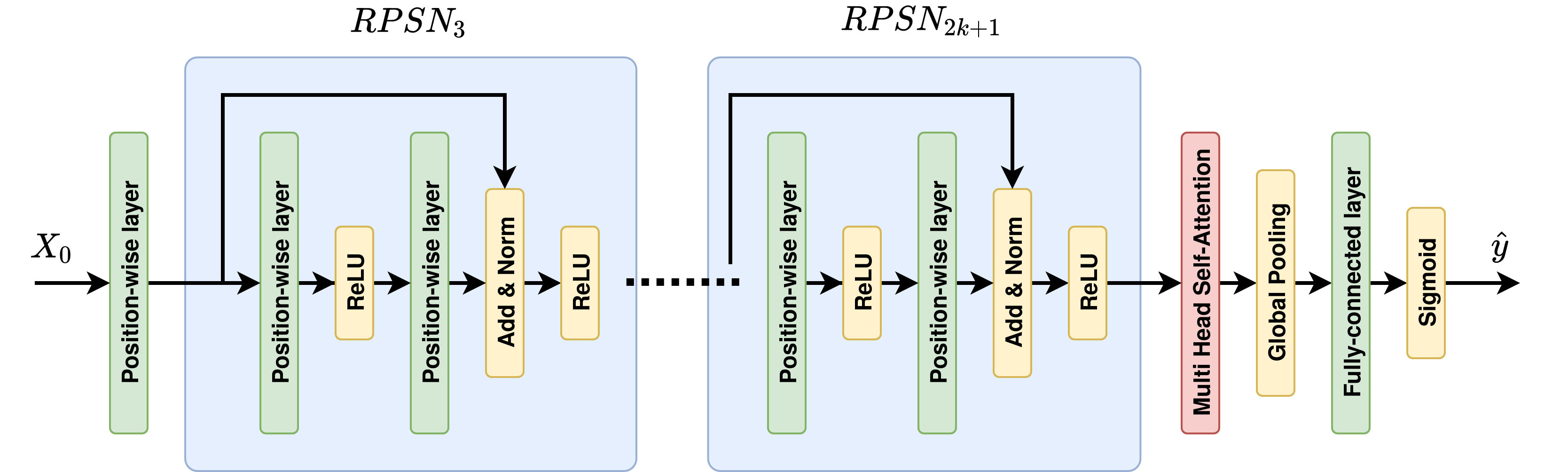
Figure 4: COLD architecture layout. Dropout is not shown in this figure

In this work we wrap $h_{j}(X_{j-1})$ by a dropout function [29]:

$$h_{d,j}=Dropout_{j}(h_{j}(X_{j-1}))$$ (2)

Putting ReLU activation, Layer Normalization [30] and the equation 2 together a function that Residual Position-Wise Sub-Networks computes can be written as follows:

$$RPSN_{j+1}(X_{j-1})=(ReLU\circ Norm\circ\hat{h}_{d,j+1})(X_{j-1})$$

Thus, the neural network proposed can be described by the following function:

$$f(X_{0})=(Pred\circ g\circ MHSA\circ RPSN_{2k+1}\circ RPSN_{2k-1}\circ\ldots\\ \ldots\circ RPSN_{3}\circ h_{1})(X_{0})$$

Then $<q,k,n_{head},p_{d}>$ is parameters space of the architecture proposed, where $k$ is a number of Residual Position-wise Sub-Networks; $p_{d}$ is a probability of dropout.

IV Model evaluation

IV-A Input data format

Spectrograms from each aggregated signal (Fig. 5) in $S_{train}$, $S_{val}$ and $S_{test}$ were obtained with use of Short Time Fourier Transform were obtained (Fig. 6). We set the window size for Fourier transform to 5 periods (0.1 second), the time between each successive windows to 1 period (0.02 sec). These parameters allow extracting spectrograms of sizes $t\times v=251\times 201$. We decided to set relatively high time dimension of the spectrogram to aggregate more information from transient processes. Thus, the spectrogram is an input matrix $X_{0}$.

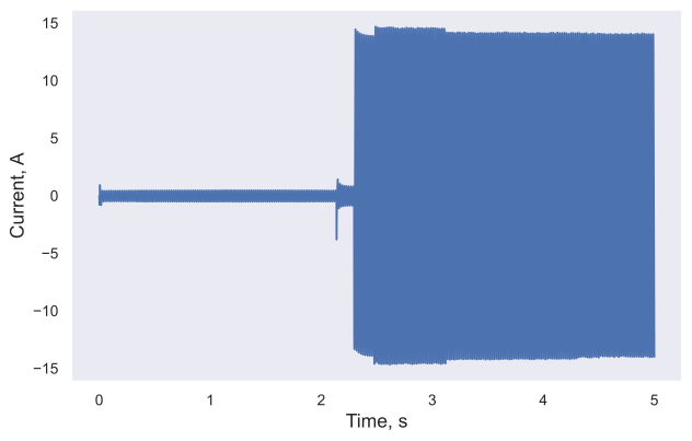
Figure 5: The example of the aggregated signal produced by the 6 appliances: cable receiver, charger, game console, light bulb, sewing machine, stove.

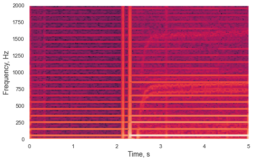
Figure 6: The spectrogram of the signal presented in Fig. 5

IV-B Loss function

To train a neural network model it is necessarily to define the function computing the error between actual output $\hat{y}$ and the desired response $y$. In this work the binary cross-entropy loss was used:

$$\mathcal{L}(y,\hat{y})=-\frac{1}{|L|}\sum_{l\in L}[y_{l}\log_{2}(\hat{y}_{l})+(1-y_{l})\log_{2}(1-\hat{y}_{l})]$$

where vectors $\hat{y}\in\mathbb{R}^{|L|}$ and $y\in(\mathbb{Z}_{2}^{+})^{|L|}$ are considered as indicators of a particular category (label) of appliances being detected within the observable interval of time.

IV-C Evaluation metric

To estimate the quality of disaggregation of concurrent loads the example-based (mean) F1-score will be applied. This metric is being calculated for pairs of a particular predicted vector $\hat{y}$ and ground-truth (desired) $y$ and then averaged over all these pairs. The choice of example-based metric is due to the multi-label classification statement of a problem. F1-score computes harmonic mean of precision and recall for a particular predicted vector $\hat{y}$ corresponding to subset $S_{w}$:

$$F1_{w}=\frac{PR_{w}\times RE_{w}}{PR_{w}+RE_{w}}$$

where $PR$ is a precision and $RE$ is a recall. The precision is a number of True Positives ($TP$) over the number of True Positives ($TP$) plus the number of False Positives ($FP$):

$$PR=\frac{TP}{TP+FP}$$

In its turn, True Positives (sensitivity) $TP$ - number of loads correctly identified as switched on; False Positives (fall-out) $FP$ - number of loads identified as switched on, while they were inactive.

The recall is a number of True Positives ($TP$) over the number of True Positives ($TP$) plus the number of False Negatives ($FN$):

$$RE=\frac{TP}{TP+FN}$$

where False Negatives (miss rate) $FN$ - number of loads identified as switched off, while they were active;

Averaging $F1_{w}$ over all predicted $\hat{y}$ for $S_{w}$ will give mean F1-score:

$$Mean\ F1_{w}=\frac{1}{|S_{w}|}\sum_{i\in[\#S_{w}]}F1_{w,i}$$

by $\#\cdot$ we denote cardinality $|\cdot|$.

Assume that $S$ comprises $W=\{w\}$ the weighted averaging should be also applied:

$$Weighted\ mF1=\sum_{w\in W}\frac{|S_{w}|}{|S|}mF1_{w}$$

Since the values of predicted vector $\hat{y}$ are probabilities of each label being detected, the decision threshold should be defined. The threshold is needed to round the real values to 1 if they are above the threshold, and to 0 otherwise. To find an optimal one a tune procedure can be performed, that is for thresholds in interval $(0,1)$ compute $weighted\ mean\ F1$, then pick the threshold that corresponds to the highest value of the metric.

V Results

As soon as it is not clear which values of $q,k,n_{head},p_{d}$ are suitable for our case the hyperparameters search should be performed. We used the ASHA algorithm [31] to iterate through the parameters space and different learning rate parameters $\{\eta\}$, weight decays $\{\lambda\}$ and mini-batch sizes $\{B\}$. This algorithm applies the aggressive strategy to stop training the models which are weaker than the others. Thus, hundreds of training procedures for different hyperparameters can be finished extremely fast in comparison to the standard grid search or random search strategies [32].

At each training step the validation procedure was performed on validating dataset $S_{val}$. It allows estimating the quality of disaggregation over the training time via weighted mean F1-score. The evaluation results at this stage are main criterion to select the hyperparameters. The ASHA algorithm was run over 100 combinations of parameters and produced the following optimal hyperparameters of the architecture proposed: $q=256$, $k=14$, $n_{head}=8$, $p_{d}=0.2$, $\eta=3\cdot 10^{-4}$, $\lambda=2.8\cdot 10^{-2}$ and $B=64$.

After finding the optimal architecture the testing procedure on $S_{test}$ needs to be applied. The idea is to understand how effective our model for real-world applications is. About 100k previously unseen examples were passed through the trained neural network for the evaluation. We computed mean F1-score for each $w$-subset of $S_{test}$ and plotted this distribution in Fig. 7. The corresponding weighted mean F1-score is $78.95\%$ at optimal threshold $0.74$. As it was noted in the Section II we did not consider $w\in\{1,2,5,7,9\}$ to avoid the memorizing of combinations. As a result, the mean F1-score for $w>2$ decreases monotonically. That is, the neural network has an interpolation property. The model has the highest mean F1-score $91.47\%$ at $w=2$. The identification of single appliances ($w=1$) is weaker due to the higher number of false positives (FP). The reason for that is the threshold tuning procedure. Since there is a weighted average over all $w$ and the size of $S_{1}$ is smallest one, therefore, the threshold has a bias towards the $w$-subsets with a higher number of examples.

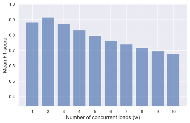
Figure 7: Weighted mean F1-score across different numbers of concurrent loads

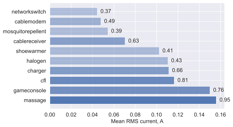
Figure 8: Top 10 categories of appliances with lowest RMS values of a current. The values near the bins and opacity correspond to F1-scores

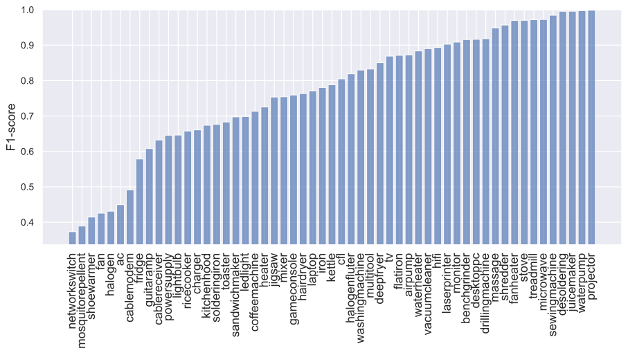
Figure 9: F1-score across different appliances (weighted over w-subsets of $S_{test}$)

It is also important to check the distribution of F1-score over the different types of loads. Fig. 9 shows F1-score across all categories of appliances. There are 7 devices with the lowest F1-score: network switch, mosquito repellent, shoe warmer, halogen, cable modem, fan and air conditioner. The possible justification can be related to the magnitudes of corresponding signals. Indeed, the analysis of baseline dataset $P$ shows that 5 out of 7 of these appliances have the lowest values of RMS current averaged over corresponding signatures (Fig. 8). We hypothesize that these signatures have no such expressive patterns as the charger or cable receiver to be detected among the loads with larger magnitudes of current. The patterns of the ”fan” category are sinusoidal and similar to other categories such as ”water heater”, ”kettle”, ”fan heater”, ”stove” etc. The detection of sinusoidal signals is a complex problem since their sum will give also a sinusoidal signal. The only way to separate them one from the others is to rely on phase shifts and transient processes. In our case, even the transient processes of the ”fan” category with mean peak RMS current value 0.73 A did not contribute to the total load consisting of such appliances as water heater (11.26 A), kettle (11.81 A) etc. As for the category ”air conditioner” we leave the issue on identification of this appliance open.

VI Discussion

TABLE VII: Comparison of approaches

Approach	Dataset	Time-scale	# Labels	$w_{max}$	F1-score	Threshold
Faustine et al. [11]	PLAID (aggregated)	short-term	12	3	94.00% (macro)	0.5
Yang et al. [23]	UK-DALE (house 1)	long-term	5	4	93.8% (macro)	0.5
Ours	Synthesized via SNS	short-term	11	3	92.39% (weighted&mean)	0.6531
Ours	Synthesized via SNS	short-term	5	4	94.55% (weighted&mean)	0.5510
Ours	Synthesized via SNS	short-term	55	10	78.95% (weighted&mean)	0.7347

We compared our approach with two previous state-of-the-art methods based on convolutional neural networks [11, 23]. The former method performed on a PLAID subset of aggregated measurements comprises $\#L=12$ different categories of appliances where maximum number of concurrent appliances is $w_{max}=3$. The latter method was evaluated at 5 and 4 appliances of the UK-DALE and REDD datasets respectively. Our analysis showed that 4 of them appeared in simultaneous work. These approaches were selected as they provide significant F1 measure, the maximum of concurrent loads and the implementation details are clear.

To make our approach comparable with the methods described we generated additional synthetic data for both cases. Version of the PLAID dataset used by [11] comprises ”fridge defroster” and ”fridge” categories of appliances as different, while in our version of the PLAID dataset they were assigned to the single category ”fridge”. For this case we synthesized train, validation and test datasets for $w=1..3$. The method [23] used ”dish washer” category of appliances which is absent in our dataset. To keep the number of available appliances we added ”vacuum cleaner” category and synthesized train, validation and test datasets for $w=1..4$. Note, that we added additional category only for the second case as the nature of these appliances is different, while the fridge and defroster, indeed, can be assigned to a common category. The optimal architectures for both cases were searched as it was described in the previous section. The source code of all the experiments is in our repository. Table VII summarizes the experiments. F1 measure used by the authors [11, 23] is macro metric, that is averaged over all labels (categories) without additional averaging over $w$. In its turn, we used metrics described in the Section IV.

One can note that this is not fair comparison as the other researchers used at least different datasets. However, some conclusions can be done: (i) the datasets produced by the SNS algorithm allow training the neural networks with classification performances at least as powerful as the models trained on fully real-world measurements; (ii) the SNS algorithm is able to simulate a consumption by a higher number of concurrent loads where the number of training examples bounded by a number of combinations of appliances and their patterns. The flexibility of the algorithm makes us possible to grow the train dataset in order to reach bounds on classification metrics of the model. Moreover, it is also possible to test the model on the much higher number of unseen examples. In real-world datasets taking a higher number of test examples will reduce the train dataset, therefore, accuracy might be lower; (iii) the architecture proposed able to disaggregate more appliances rather than previous approaches. However, the F1-score decreases significantly with a growing number of concurrent loads. Additional data points might be added to $S_{test}$ to improve the generalization ability of the model.

VII Conclusion

In this research, we have proposed the SNS algorithm with flexible hyperparameters. This gives a wide range of advantages for the NILM researchers. We showed that relatively small amount of individual measurements of appliances can be turned into the large dataset of simulated aggregated measurements. The data collection process can be reduced significantly. However, our algorithm works only with short-term patterns. But the use of short-term current patterns can lead to real-time applications of the NILM (per-second analysis). The SNS algorithm can produce synthetic data to train the model for any number of concurrent loads. We showed that taking advantage of the synthetic dataset comprised up to 10 simultaneously working devices it is possible to train the neural network with weighted mean F1-score up to $79\%$. This kind of performance meets the lower bound for real-world applications [2]. We developed the COLD architecture which is based on the theoretically justified ReLU network and recent state-of-the-art mechanism named multi-head self attention to account time-dependency in the input data, and therefore, improve the performance on large amount of unseen (test) examples. However, our approach has a drawback: we used prefiltered measurements from the WHITED and PLAID datasets without any augmentation technique. Therefore, our model is not robust to the noisy data. We are going to fill this gap in our further work. Another important task planned to attain next is to validate our model on real-world measurements without additional training of the model.

June 4, 2021

References

- [1] G. Hart, “Nonintrusive appliance load monitoring,” Proceedings of the IEEE, vol. 80, no. 12, pp. 1870–1891, 1992.
- [2] M. Zhuang, M. Shahidehpour, and Z. Li, “An overview of non-intrusive load monitoring: Approaches, business applications, and challenges,” in 2018 International Conference on Power System Technology (POWERCON), 2018, pp. 4291–4299.
- [3] L. Mauch and B. Yang, “A new approach for supervised power disaggregation by using a deep recurrent lstm network,” in 2015 IEEE Global Conference on Signal and Information Processing (GlobalSIP), 2015, pp. 63–67.
- [4] H. Liu, Q. Zou, and Z. Zhang, “Energy disaggregation of appliances consumptions using ham approach,” IEEE Access, vol. 7, pp. 185 977–185 990, 2019.
- [5] L. Jiang, S. Luo, and J. Li, “An approach of household power appliance monitoring based on machine learning,” in 2012 Fifth International Conference on Intelligent Computation Technology and Automation, 2012, pp. 577–580.
- [6] H. Liu, Q. Zou, and Z. Zhang, “Energy disaggregation of appliances consumptions using ham approach,” IEEE Access, vol. 7, pp. 185 977–185 990, 2019.
- [7] A. Faustine, L. Pereira, H. Bousbiat, and S. Kulkarni, “Unet-nilm: A deep neural network for multi-tasks appliances state detection and power estimation in nilm,” in Proceedings of the 5th International Workshop on Non-Intrusive Load Monitoring, ser. NILM’20. New York, NY, USA: Association for Computing Machinery, 2020, p. 84–88. [Online]. Available: https://doi.org/10.1145/3427771.3427859
- [8] D. Yang, X. Gao, L. Kong, Y. Pang, and B. Zhou, “An event-driven convolutional neural architecture for non-intrusive load monitoring of residential appliance,” IEEE Transactions on Consumer Electronics, vol. 66, no. 2, pp. 173–182, 2020.
- [9] L. Massidda, M. Marrocu, and S. Manca, “Non-intrusive load disaggregation by convolutional neural network and multilabel classification,” Applied Sciences, vol. 10, no. 4, p. 1454, Feb 2020. [Online]. Available: http://dx.doi.org/10.3390/app10041454
- [10] D. Yang, X. Gao, L. Kong, Y. Pang, and B. Zhou, “An event-driven convolutional neural architecture for non-intrusive load monitoring of residential appliance,” IEEE Transactions on Consumer Electronics, vol. 66, no. 2, pp. 173–182, 2020.
- [11] A. Faustine and L. Pereira, “Multi-label learning for appliance recognition in nilm using fryze-current decomposition and convolutional neural network,” Energies, vol. 13, no. 16, p. 4154, Aug 2020. [Online]. Available: http://dx.doi.org/10.3390/en13164154
- [12] P. A. Lindahl, D. H. Green, G. Bredariol, A. Aboulian, J. S. Donnal, and S. B. Leeb, “Shipboard fault detection through nonintrusive load monitoring: A case study,” IEEE Sensors Journal, vol. 18, no. 21, pp. 8986–8995, 2018.
- [13] Z. D. Tekler, R. Low, Y. Zhou, C. Yuen, L. Blessing, and C. Spanos, “Near-real-time plug load identification using low-frequency power data in office spaces: Experiments and applications,” Applied Energy, vol. 275, p. 115391, 2020.
- [14] T. Le, H. Kang, and H. Kim, “Household appliance classification using lower odd-numbered harmonics and the bagging decision tree,” IEEE Access, vol. 8, pp. 55 937–55 952, 2020.
- [15] M. Kahl, A. Ul Haq, T. Kriechbaumer, and H.-A. Jacobsen, “A comprehensive feature study for appliance recognition on high frequency energy data,” in Proceedings of the Eighth International Conference on Future Energy Systems, ser. e-Energy ’17. New York, NY, USA: Association for Computing Machinery, 2017, p. 121–131. [Online]. Available: https://doi.org/10.1145/3077839.3077845
- [16] P. Cunningham and S. J. Delany, “k-nearest neighbour classifiers: 2nd edition (with python examples),” 2020.
- [17] C. J. C. Burges, “A tutorial on support vector machines for pattern recognition,” Data Min. Knowl. Discov., vol. 2, no. 2, p. 121–167, Jun. 1998. [Online]. Available: https://doi.org/10.1023/A:1009715923555
- [18] J. Kelly and W. Knottenbelt, “The uk-dale dataset, domestic appliance-level electricity demand and whole-house demand from five uk homes,” Scientific data, vol. 2, no. 1, pp. 1–14, 2015.
- [19] J. Z. Kolter and M. J. Johnson, “Redd: A public data set for energy disaggregation research,” in Workshop on data mining applications in sustainability (SIGKDD), San Diego, CA, vol. 25, no. Citeseer, 2011, pp. 59–62.
- [20] J. Gao, S. Giri, E. C. Kara, and M. Bergés, “Plaid: a public dataset of high-resoultion electrical appliance measurements for load identification research: demo abstract,” in proceedings of the 1st ACM Conference on Embedded Systems for Energy-Efficient Buildings, 2014, pp. 198–199.
- [21] M. Kahl, A. U. Haq, T. Kriechbaumer, and H.-A. Jacobsen, “Whited-a worldwide household and industry transient energy data set,” in 3rd International Workshop on Non-Intrusive Load Monitoring, 2016, pp. 1–4.
- [22] J. Kelly and W. Knottenbelt, “Neural nilm: Deep neural networks applied to energy disaggregation,” in Proceedings of the 2nd ACM international conference on embedded systems for energy-efficient built environments, 2015, pp. 55–64.
- [23] Y. Yang, J. Zhong, W. Li, T. A. Gulliver, and S. Li, “Semisupervised multilabel deep learning based nonintrusive load monitoring in smart grids,” IEEE Transactions on Industrial Informatics, vol. 16, no. 11, pp. 6892–6902, 2020.
- [24] P. Huber, A. Calatroni, A. Rumsch, and A. Paice, “Review on deep neural networks applied to low-frequency nilm,” Energies, vol. 14, no. 9, p. 2390, 2021.
- [25] B. Hanin and M. Sellke, “Approximating continuous functions by relu nets of minimal width,” 2018.
- [26] A. Vaswani, N. Shazeer, N. Parmar, J. Uszkoreit, L. Jones, A. N. Gomez, L. Kaiser, and I. Polosukhin, “Attention is all you need,” 2017.
- [27] B. McFee, C. Raffel, D. Liang, D. P. Ellis, M. McVicar, E. Battenberg, and O. Nieto, “librosa: Audio and music signal analysis in python,” in Proceedings of the 14th python in science conference, vol. 8, 2015.
- [28] K. He, X. Zhang, S. Ren, and J. Sun, “Deep residual learning for image recognition,” 2015.
- [29] N. Srivastava, G. Hinton, A. Krizhevsky, I. Sutskever, and R. Salakhutdinov, “Dropout: A simple way to prevent neural networks from overfitting,” J. Mach. Learn. Res., vol. 15, no. 1, p. 1929–1958, Jan. 2014.
- [30] J. L. Ba, J. R. Kiros, and G. E. Hinton, “Layer normalization,” 2016.
- [31] L. Li, K. Jamieson, A. Rostamizadeh, E. Gonina, M. Hardt, B. Recht, and A. Talwalkar, “A system for massively parallel hyperparameter tuning,” 2020.
- [32] J. Bergstra and Y. Bengio, “Random search for hyper-parameter optimization,” Journal of Machine Learning Research, vol. 13, no. 10, pp. 281–305, 2012. [Online]. Available: http://jmlr.org/papers/v13/bergstra12a.html