Parallel and External-Memory Construction of
Minimal Perfect Hash Functions with PTHash

Abstract

A function $f:U\to\{0,\ldots,n-1\}$ is a minimal perfect hash function for a set $S\subseteq U$ of size $n$, if $f$ bijectively maps $S$ into the first $n$ natural numbers. These functions are important for many practical applications in computing, such as search engines, computer networks, and databases. Several algorithms have been proposed to build minimal perfect hash functions that: scale well to large sets, retain fast evaluation time, and take very little space, e.g., 2 – 3 bits/key. PTHash is one such algorithm, achieving very fast evaluation in compressed space, typically many times faster than other techniques. In this work, we propose a new construction algorithm for PTHash enabling: (1) multi-threading, to either build functions more quickly or more space-efficiently, and (2) external-memory processing, to scale to inputs much larger than the available internal memory. Only few other algorithms in the literature share these features, despite of their practical impact. We conduct an extensive experimental assessment on large real-world string collections and show that, with respect to other techniques, PTHash is competitive in construction time and space consumption, but retains 2 – 6$\times$ better lookup time.

1 Introduction

Minimal perfect hashing (MPH) is a well-studied and fundamental problem in Computer Science. It asks to build a data structure mapping the $n$ keys of a set $S$ out of a universe $U$ into the numbers $[n]=\{0,\ldots,n-1\}$. In other words, the resulting data structure realizes a “one-to-one” correspondence between $S$ and the integers in $[n]$. Such a function $f:U\rightarrow\{0,\ldots,n-1\}$ is called a minimal perfect hash function (MPHF henceforth) for $S$.

MPHFs are useful in all those practical situations where space-efficient storage and fast retrieval from static sets is a primary concern. In fact, they are employed in compressed full-text indexes [1], computer networks [2], databases [3], prefix-search data structures [4], language models [5, 6], indexes for DNA [7, 8, 9], Bloom filters and their variants [10, 11, 12], and many other applications.

The most interesting aspect of the MPH problem is that it ignores the behavior of $f$ on keys that do not belong to $S$, i.e., $f(x)$ can be any value in $[n]$ if $x\in U\setminus S$. Therefore, the MPHF data structure does not need to store the keys. As a result, pioneer work on the problem has proved a space lower bound of $n\log_{2}(e)$ bits for the size of any MPHF [13, 14], which is approximately just 1.442 bits/key. While it is difficult to come close to this space usage, several practical algorithms exist that take little space, i.e., 2 – 3 bits/key, retain very fast lookup time, and scale well to large sets, e.g., billions of keys.

Our initial investigation on the problem was motivated by the observation that MPHFs are usually built once and evaluated many times, thus making lookup time the most critical aspect for the MPH problem, provided that both construction time and space usage are reasonably low. To this end, we proposed PTHash [15], which is significantly faster at lookup time than other techniques while taking a similar memory footprint. In our previous work, however, we only proposed a sequential and internal-memory construction.

In this work, we extend the treatment of PTHash and consider two important algorithmic aspects: multi-threading and external-memory processing. While multi-threading can be used to either quicken the construction or build more space-efficient functions, temporary disk storage can be used to scale to inputs much larger than the available internal memory. Only few other algorithms in the literature support these two features, despite of their practical impact.

A simple and elegant solution to harness both aspects is to partition the input and build, in internal memory, an independent MPHF on each partition [16]. This approach also offers good scalability as the independent partitions that fit into internal memory may be processed in parallel by multiple threads. Very importantly, this solution is valid for any construction algorithm. However, this approach imposes an indirection at lookup time to identify the partition, i.e., the proper MPHF to query, and additional space to store the offset of each partition. Indeed, partitioned MPHFs are usually $30-50\%$ slower and $20\%$ larger than their non-partitioned counterpart [16, 17].

Our Contribution

Since the construction can either use one or multiple threads and can either run in internal or external memory, we consider the four possible construction settings: sequential internal-memory, parallel internal-memory, sequential external-memory, parallel external-memory.

We present a new construction algorithm for PTHash that overcomes the overhead of the folklore partitioning approach and, yet, easily adapts to all of the above four settings. We conduct an extensive experimental assessment over real-world string collections, ranging in size from tens of millions to several billions of strings. We show that PTHash is competitive at building MPHFs with the best existing techniques that also support parallel execution and external-memory processing. However, and very importantly, PTHash retains the best lookup time being 2 – 6 times faster than other techniques. Our C++ MPHF library is publicly available at https://github.com/jermp/pthash.

Organization

The article is structured as follows. Section 2 reviews all the practical approaches for MPH and indicates which techniques support multi-threading and/or use external memory. Section 3 presents a new general PTHash construction algorithm, with Section 4 describing how its design seamlessly adapts to the different settings we consider. In particular, Section 4.2 and 4.3 detail how the general construction works in internal and external memory, respectively, with multi-threading support (Section 4.1). Section 5 presents experimental results, in comparison with the approaches reviewed in Section 2. We conclude in Section 6.

2 Related Work

Minimum perfect hashing has a long development history. Our focus is on practical approaches that have been implemented and shown to perform well on large key sets. Indeed, we point out that some theoretical constructions, like that by Hagerup and Tholey [18], achieve the space lower bound of $n\log_{2}(e)$ bits, but only work in the asymptotic sense, i.e., for $n$ too large to be of any practical interest.

Up to date, four “classes” of different, practical, approaches have been devised to solve the problem, which we describe below in chronological order of proposal. Table I summarizes the notation used to describe all algorithms while Table II shows the theoretical construction times and the implementation aspects of each algorithm.

Hash and Displace

The hash and displace technique was originally introduced by Fox, Chen, and Heath [19] in a work that was named FCH after them. That work also inspired the development of PTHash [15]. The main idea of the algorithm is as follows.

Keys are first hashed and mapped into $\lceil cn/\log_{2}(n)\rceil$ non-uniform buckets, for a given parameter $c>\log_{2}(e)$; the buckets are then sorted and processed by falling size: for each bucket, a displacement value $d_{i}\in[n]$ is determined so that all keys in the bucket can be placed without collisions to positions $(h(x)+d_{i})\,\textup{mod}{\,n}$, using a random hash function $h$. Lastly, the sequence of displacements $d_{i}$ is stored in compact form using $\lceil\log_{2}(n)\rceil$ bits per value. While the theoretical analysis suggests that by decreasing the number of buckets it is possible to lower the space usage, at the cost of a larger construction time, in practice it is unfeasible to go below 2.5 bits/key for large values of $n$.

In the compressed hash and displace (CHD) variant by Belazzougui et al. [20], keys are first uniformly distributed to $\lceil n/\lambda\rceil$ buckets, for a given parameter $\lambda\geq 1$. The buckets are then sorted and processed by falling size: for each bucket, a pair of displacements $\langle d_{0},d_{1}\rangle$ is determined so that all keys in the bucket can be placed without collisions to positions $(h_{1}(x)+d_{0}h_{2}(x)+d_{1})\,\textup{mod}{\,N}$ using a pair of random hash functions $(h_{1},h_{2})$, with $N=(1+\varepsilon)\cdot n$ slots, for a given parameter $\varepsilon>0$. Instead of storing a pair $\langle d_{0},d_{1}\rangle$ for each bucket, CHD stores the index of such pair in the sequence

$$\langle 0,0\rangle,\ldots,\langle 0,N-1\rangle,\ldots,\langle N-1,0\rangle,\ldots,\langle N-1,N-1\rangle.$$

The sequence of indexes is stored in compressed form using an entropy coding mechanism with $O(1)$ access time [21].

TABLE I: General notation (upper) and PTHash-specific notation (bottom).

$S$	set of keys
$n$	number of keys in $S$, $n=|S|$
$[n]$	$\{0,\ldots,n-1\}$
$f$	MPHF built from $S$
$f(x)$	a value in $[n]$, the result of computing $f$ on the key $x$
$h$	a fully random hash function
$c$	value that trades search efficiency for space effectiveness
$\alpha$	value in $(0,1)$, used to define the search space $\left[N=\lceil n/\alpha\rceil\right]$
$m$	number of buckets used for the search, $m=\lceil cn/\log_{2}\left(n\right)\rceil$
$L$	largest bucket size
$P$	pilots table
$x\oplus y$	bitwise XOR between hash codes $x$ and $y$

TABLE II: Theoretical construction time and implementation details.

Algorithm	Construction Time	Implementation
		multi-thr.	ext. mem.
PTHash	$O\big{(}n^{1+\Theta(\alpha/c)}\big{)}$	$\checkmark$	$\checkmark$
FCH	not reported
CHD	$O\big{(}n\cdot(2^{\lambda}+(1/\varepsilon)^{\lambda})\big{)}$
EMPHF, GOV	$O(n)$		$\checkmark$
BBHash	$O(n\cdot e^{1/\gamma})$	$\checkmark$	$\checkmark$
RecSplit	$O(n)$

Linear Systems

In the late 90s, Majewski et al. [22] introduced an algorithm to build a MPHF exploiting a connection between linear systems and hypergraphs. Almost ten years later, Chazelle et al. [23] proposed an analogous construction in an independent manner. The MPHF $f$ is found by generating a system of $n$ random equations in $t$ variables of the form

$$f(x)=w_{h_{1}(x)\,\textup{mod}{\,t}}+\cdots+w_{h_{r}(x)\,\textup{mod}{\,t}}\,\textup{mod}{\,n},\text{ for }x\in S,$$

where $\{h_{i}\}_{i\in[r]}$ are $r$ random hash functions and $\{w_{i}\}_{i\in[t]}$ are $t$ variables whose values are in $[n]$. Due to bounds on the acyclicity of random graphs, the system can be triangulated with high probability and solved in linear time by peeling the corresponding hypergraph if the ratio between $t$ and $n$ is above a certain threshold $\gamma_{r}$. The constant $\gamma_{r}$ depends on the degree $r$ of the graph and attains its minimum for $r=3$, where the value is $\gamma_{3}\approx 1.23$, i.e., the system consists of $n$ equations of $3$ terms in $\lceil 1.23n\rceil$ variables. Recently, Dietzfelbinger and Walzer [24] described a new family of random hypergraphs, called fuse graphs, that are peelable with high probability even when the edge density is close to 1. Practically, this reduces the space overhead of any solution based on linear systems from 23% to 12%. Additional savings are possible using $r>3$ hash functions at the expense of increasing the construction time.

Belazzougui et al. [17] proposed a cache-oblivious implementation of the previous algorithm suitable for external memory construction and named EMPHF. The algorithm employs a compact representation of the incidence lists of the hypergraph, which is based on the observation that it is not necessary to store actual edges. Instead, all vertices in the same position can be XORed together, hence a constant amount of memory per node is retained.

Genuzio et al. [25, 26] (GOV) demonstrated practical improvements to the Gaussian elimination technique, which is used to solve the linear system. The improvements are based on broadword programming techniques. The authors released a very efficient implementation of the algorithm that scales well using external memory and multi-threading.

Fingerprinting

Müller et al. [27] introduced a technique based on fingerprinting. The general idea is as follows. All keys are first hashed in $[n]$ using a random hash function, then collisions are recorded using a bitmap $B_{0}$ of size $n_{0}=n$. In particular, keys that do not collide have their position in the bitmap marked with a 1; all positions involved in a collision are marked with a 0 instead. If $n_{1}>0$ collisions are produced, then the same process is repeated recursively for the $n_{1}$ colliding keys using a bitmap $B_{1}$ of size $n_{1}$. All bitmaps, called “levels”, are then concatenated together in a bitmap $B$. The lookup algorithm keeps hashing the key level by level until a 1 is hit, say in position $p$ of $B$. A constant-time ranking data structure [28] is used to count the number of 1s in $B[0..p]$ to ensure that the returned value is in $[n]$. On average, only $1.56$ levels are accessed in the most succinct setting [27], which takes 3 bits/key.

Limasset et al. [29] provided an implementation of this approach, named BBHash, that is very fast in construction and scales to very large key sets using multi-threading and external-memory processing. Furthermore, no auxiliary data structures are needed during construction except the levels themselves, meaning that the space consumed in the process is essentially that of the final MPHF. The authors also introduced a parameter $\gamma\geq 1$ to speedup construction and lookup time by using bitmaps that are $\gamma$ times bigger at any level. This clearly reduces collisions and, thus, the average number of levels accessed per lookup. However, the larger $\gamma$, the higher the space consumption.

Recursive Splitting

Esposito et al. [30] proposed a recursive splitting algorithm (RecSplit) to build very succinct functions, e.g., 1.80 bits/key, in expected linear time. Also, it provides fast lookup time in expected constant time. The authors first observed that, for very small sets, it is possible to find a MPHF simply by brute-force searching for a bijection with a suitable codomain. Then, the same approach is applied in a divide-and-conquer manner to solve the problem on larger inputs.

Given two parameters $b$ and $\ell$, the keys are divided into buckets of average size $b$ using a random hash function. Each bucket is recursively split until a block of size $\ell$ is formed and for which a MPHF can be found using brute-force, hence forming a rooted tree of splittings. The parameters $b$ and $\ell$ provide different space/time trade-offs. While providing a very compact representation, the evaluation performs one memory access for each level of the tree that penalizes the lookup time.

The authors indicate that the approach is amenable to good parallelization as the buckets may be processed by multiple threads in parallel. However, at the time of writing, there is no public parallel implementation of this algorithm.

3 A General Construction

This section presents a general construction algorithm for PTHash, based on a few abstract steps, that is suitable for both the parallel and external-memory settings. While the focus of this section is on the algorithm rather than on the specific implementation, Section 4 will detail how the proposed construction can be easily implemented in practice to support the different settings.

At a high level, the construction first hashes and maps the keys into non-uniform buckets, then processes the buckets in decreasing order of size: for each bucket, an integer $k_{i}$ – the pilot of the $i$-th bucket – is determined so that all keys in the bucket can be placed without collisions to positions

$$f(x)=(h(x)\oplus h(k_{i}))\,\textup{mod}{\,n}$$

where $h$ is a random hash function. Lastly, the sequence of such pilots, one for each bucket, is materialized in a pilots table (PT), indicated with $P$ throughout the paper. The table is stored in compressed format using a compressor supporting random access to $P[i]$ in $O(1)$ worst-case time.

1 Build($S$, $c$, $\alpha$)

2       $\mbox{\emph{blocks}}=\textsc{Map}(S,c)$

3       $\mbox{\emph{buckets}}=\textsc{Merge}(\mbox{\emph{blocks}})$

4       $P=\textsc{Search}(\mbox{\emph{buckets}},n/\alpha)$

5       $\textsc{Encode}(P)$

6      

7

Alg. 1 The general construction algorithm for a set $S$ of $n$ keys, and parameters $c$ and $\alpha$.

Besides the input set $S$, the construction employs two parameters, $c>\log_{2}(e)$ and $0<\alpha<1$, respectively affecting the number of buckets and the size of the search space – refer to the bottom part of Table I for the notation used to describe PTHash. The general construction algorithm is composed of three steps, namely Map, Merge, and Search, followed by an Encode step that compresses the table as anticipated before. These steps, explained in the following, are summarized in Alg. 1.

3.1 Map

The first step aims at mapping each key of $S$ to a fixed number of bytes using a random hash function $h$. During this step, keys are “logically” associated to one of the $m=\lceil cn/\log_{2}(n)\rceil$ buckets $\{B_{0},\ldots,B_{m-1}\}$, that are indicated with the integers in $[0..m-1]$. Specifically, the bucket identifier for a key $x$ is obtained via the function

$$\mbox{bucket}(x)=\left\{\begin{array}[]{ll}h^{\prime}(x)\,\textup{mod}{\,p_{2}}&h^{\prime}(x)\,\textup{mod}{\,n}<p_{1}\\ h^{\prime}(x)\,\textup{mod}{\,(m-p_{2})}+p_{2}&\mbox{otherwise}\\ \end{array}\right.$$

where $h^{\prime}$ is a random hash function, like $h$, while $p_{1}$ and $p_{2}$ are two thresholds set to, respectively, $\frac{6}{10}n$ and $\frac{3}{10}m$ so that the mapping of keys into buckets is uneven: roughly 60% of the keys are mapped into 30% of the buckets. This process induces a skewed distribution of the bucket sizes, as depicted in the example of Fig. 1a. The example – for $n=10^{6}$ keys and $c=3.5$ – shows the percentage of buckets that have size equal to $|B|$, for $|B|=L,\ldots,1$, with $L=28$ being the largest bucket size. As evident, large buckets are very few while most of them are small. Such skewed distribution of keys into buckets is very important for the efficiency of the Search step and for the final compression effectiveness, as we are going to motivate in Section 3.3.

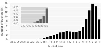
(a)

(b)

Figure 1: Bucket size distribution and load factor as buckets are processed by decreasing size order, for $n=10^{6}$ keys, $\alpha=0.94$, and $c=3.5$.

For each key $x\in S$ we generate an integer pair

$$\langle\mbox{\emph{id}},\mbox{\emph{hash}}\rangle=\langle\mbox{bucket}(x),h(x)\rangle$$

and divide the $n$ pairs into $K$ blocks, each of (roughly) equal size. The pairs in each block are sorted by, first, the id component, then by hash. Blocks are formed either because: keys are evenly distributed among $K$ threads and processed in parallel in internal memory, or a block of pairs is flushed to disk when internal memory is exhausted. We will better explain these two scenarios in Section 4.2 and 4.3.

The Map step takes $O(n\log(n/K))$ expected time using quick-sort and assuming the computation of $h(x)$ and $h^{\prime}(x)$ to take $O(1)$ time. If we use $u$-bit hash codes, the temporary space used during this step is $n\cdot(\lceil\log_{2}(m)\rceil+u)$ bits.

3.2 Merge

The $K$ blocks output by the previous step are then merged to group together all the hash codes of each bucket. Specifically, the pairs are merged by their id component first, then by hash. In this way we are also able to check that all keys were correctly hashed to distinct hash codes. Moreover, since pairs having the same id are also sorted by hash, checking for duplicate keys is very efficient as it can be performed with a single scan.

During this step we also accomplish to sort the buckets by non-increasing size as follows. We allocate $L$ buffers. Suppose the merge for a bucket is complete and the bucket contains $k$ hash codes. We append its identifier and the $k$ hash codes to the $k$-th buffer so to have all the buckets of the same size written contiguously. Once the merge is complete, the $K$ input blocks with the pairs are destroyed.

The output of this step is the set of such $L$ buffers, so that the next step, Search, has to logically process the buffers from index $L-1$ down to index $0$. We indicate the $L$ buffers with the abstraction buckets in Alg. 1. This abstract collection buckets must only support sequential iteration in the wanted bucket order (from largest to smallest bucket size). Sequential iteration is an access pattern of crucial importance as to avoid expensive memory reads for the buckets, especially in the external-memory setting. Each element of the collection is a bucket – an object made by an array of hashes, plus a unique identifier $0\leq\mbox{\emph{id}}\leq m-1$.

The overall time complexity of Merge is $O(n\log K)$ using a min-heap data structure of size $O(K)$ memory words to merge the blocks. Since each bucket in the $k$-th buffer is a contiguous span of $k+1$ integers, for $0\leq k<L$, the total space taken by the merge step is $m\lceil\log_{2}(m)\rceil+nu+O(L)$ bits, where the last term is negligible as $L$ is very small compared to $n$, e.g., $L<40$ in our experiments with billions of keys.

1 Search(buckets, $N$)

2      

3      $P=\varnothing$

4       $\mbox{\emph{positions}}=\varnothing$

5       allocate the bitmap $\mbox{\emph{taken}}[0..N-1]$ with all 0s

6      

7      for $i=0;\,i<m;\,i=i+1$ : 

8             $\mbox{\emph{bucket}}=\mbox{\emph{buckets}}[i]$

9             $k_{i}=0$ $\triangleright$ pilot for $i$-th bucket

10             while true : 

11                  

12                  clear positions

13                   $j=0$

14                   for ; $j<|\mbox{\emph{bucket}}.\mbox{\emph{hashes}}|;\,j=j+1$ : 

15                         $p=(\mbox{\emph{bucket}}.\mbox{\emph{hashes}}[j]\oplus h(k_{i}))\,\textup{mod}{\,N}$

16                         if $\mbox{\emph{taken}}[p]=\mbox{{1}}$ : 

17                               $k_{i}=k_{i}+1$

18                               break $\triangleright$ try next pilot

19                              

20                        add $p$ to positions

21                        

22                  

23                  if $j=|\mbox{\emph{bucket}}.\mbox{\emph{hashes}}|$ : 

24                        

25                        if positions contains duplicates : 

26                               $k_{i}=k_{i}+1$

27                               continue $\triangleright$ try next pilot

28                              

29                        

30                        add $\langle\mbox{\emph{bucket}}.\mbox{\emph{id}},k_{i}\rangle$ to $P$ $\triangleright$ save pilot

31                         for all $p$ in positions : $\mbox{\emph{taken}}[p]=\mbox{{1}}$

32                        

33                        break

34                        

35                  

36            

37      

38      $\textsc{Sort}(P)$

39       return $P$

40

Alg. 2 The Search algorithm for an input collection of $m$ buckets in a search space of size $N=\lceil n/\alpha\rceil$.

3.3 Search

The Search step is the core of the whole construction and it is illustrated in Alg. 2. The algorithm keeps track of occupied positions in the search space $\left[N=\lceil n/\alpha\rceil\right]=\{0,\ldots,N-1\}$ using a bitmap of $N$ bits, $\mbox{\emph{taken}}[0..N-1]$, that initially are all set to 0. For each $\mbox{\emph{bucket}}=\mbox{\emph{buckets}}[i]$, we search for an integer $k_{i}$, called pilot of the bucket, satisfying the condition $\mbox{\emph{taken}}[p]=\mbox{{0}}$ for all positions $p=(h(x)\oplus h(k_{i}))\,\textup{mod}{\,N}$ assigned to the hashes of the bucket keys $h(x)\in\mbox{\emph{bucket}}.\mbox{\emph{hashes}}$. If the search for $k_{i}$ is successful, i.e., $k_{i}$ places all hashes of bucket into different unused positions of taken (checks of the lines 13 and 18), then $k_{i}$ is saved in the pilots table $P$ (line 21) and the positions are marked as occupied via $\mbox{\emph{taken}}[p]=\mbox{{1}}$ (line 22); otherwise, the next integer $k_{i}+1$ is tried.

At this stage of the description, $P$ is modeled as an abstract collection of pairs $\langle\mbox{\emph{id}},\mbox{\emph{pilot}}\rangle$. The collection is then sorted by id to materialize the final pilots table (line 24). In this way, the code of Search can adapt to either work in internal or external memory.

The positions $p$ (line 12) and pilots $k_{i}$ are 64-bit integers. The Search algorithm consumes $N$ bits for the bitmap taken, plus $64\cdot L$ bits for the array positions because at most $L$ positions can be added to it, plus $m\cdot(\lceil\log_{2}(m)\rceil+64)$ bits for P.

Expected Pilot Value and Search Time

Each pilot $k_{i}$ is a random variable taking value $v\in\{0,1,2,\ldots\}$ with probability depending on the current load factor of the bitmap taken (fraction of bits set). It follows that $k_{i}$ is geometrically distributed with success probability $p_{i}$ being the probability of placing all keys in $B_{i}$ without collisions. Let $\alpha(i)$ be the load factor of the bitmap after buckets $B_{0},\ldots,B_{i-1}$ have been processed, that is $\alpha(i)=\frac{\alpha}{n}\sum_{j=0}^{i-1}|B_{j}|$, for $i=1,\ldots,m$ and $\alpha(0)=0$ for convenience (empty bitmap). Since the keys are displaced using a fully random hash function, the probability $p_{i}$ can be modeled as $p_{i}=(1-\alpha(i))^{|B_{i}|}$.

Fact 1.

The expected number of trials per bucket is

$$\operatorname{\mathbb{E}}[k_{i}]+1=1/p_{i}=(1-\alpha(i))^{-|B_{i}|}.$$ (1)

Proof.

Since $k_{i}$ is geometrically distributed, $\operatorname{\mathbb{P}}(k_{i}=v)=p_{i}(1-p_{i})^{v}$ which is the probability of succeeding after $v$ failures ($v+1$ trials). Hence, $\operatorname{\mathbb{E}}[k_{i}]=1/p_{i}-1$. ∎

Fact 1 explains why the expected pilot value – thus, the expected number of trials per bucket – is small on average. In fact, Search processes the buckets in decreasing size order and the load factor is very small when the exponent $|B_{i}|$ is large, i.e., during the initial phase of the process. Then, as buckets are processed, the load factor grows and the exponent $|B_{i}|$ shrinks. Fig. 1b shows an example of how the load factor grows due to all buckets of size $\leq|B|$, for $|B|=28,\ldots,1$. Note the very slow growth rate of the load factor – e.g., it is smaller than 0.5 for $|B_{i}|\geq 10$ and higher than 0.9 only for $|B_{i}|\leq 2$.

Lastly, we give the following theorem which relates the performance of Search, in terms of expected CPU time, to the parameters $c$ and $\alpha$. See the Appendix for a proof.

Theorem 1.

The expected time of Search (Alg. 2), for $n$ keys and parameters $c>\log_{2}(e)$ and $0<\alpha<1$, is $O(n^{1+\Theta(\alpha/c)}).$

Minimal Output

The search space is $N=n/\alpha>n$ since $\alpha<1$. It makes the search for pilots faster by lowering the probability of hitting already taken positions in the bitmap. However, we now need to build a mapping of the $n$ keys from $[N]$ to $[n]$ to make $f$ minimal.

Suppose $F$ is the list of unused positions up to, and including, position $n-1$. Then, there are $|F|$ keys that can fill such unused positions which are mapped to positions $p_{i}\geq n$. To this end, we materialize an array $\mbox{\emph{free}}[0..N-n-1]$, where $\mbox{\emph{free}}[p_{i}-n]=F[i]$, for each $i=0,\ldots,|F|-1$. It allows us to easily map the keys ending outside $[n]$ to distinct unused positions of $[n]$. To compute the (uncompressed) free array we need $\Theta(n)$ time and $64\cdot(N-n)$ bits.

3.4 Encode

The PTHash data structure stores the two compressed tables, $P$ and free. For the free array, we always use Elias-Fano [32, 33], noting that it only takes

$$(N-n)(\lceil\log_{2}(n/(N-n))\rceil+2+o(1))\text{ bits.}$$

The pilots table $P$, instead, can be compressed using any compressor for integer sequences that supports constant-time random access to its $i$-th integer $P[i]$. It is also desirable that compressing $P$ runs in linear time, i.e., $\Theta(m)$ time. We thus only consider compressors with this complexity in the article.

Therefore, we have three degrees of freedom for the tuning of PTHash, namely the choice of

• the compressor for $P$,

• the size of the search space, tuned with $\alpha$, and

• the number of buckets, tuned with $c$,

that allow us to obtain different space/time trade-offs. We point the interested reader to our previous paper [15] for an overview and discussion of the achievable trade-offs. For example, a good balance between space effectiveness and lookup efficiency is obtained using the front-back dictionary-based encoding (D-D) [15], with $\alpha=0.94$ and $c=7.0$. More compact representations can be obtained, instead, by using Elias-Fano (EF) on the prefix-sums of $P$ at the price of a slowdown at query time. We are going to use both configurations in the experiments as reference points.

1 $P[i]$

2       $\mbox{\emph{block}}=\lfloor i/b\rfloor$

3       $\mbox{\emph{offset}}=i\,\textup{mod}{\,b}$

4       $w=W[\mbox{\emph{block}}+1]-W[\mbox{\emph{block}}]$

5       $position=W[\mbox{\emph{block}}]\cdot b+\mbox{\emph{offset}}\cdot w$

6       $x=B[\mbox{\emph{position}},\mbox{\emph{position}}+w]$

7       return $x$

8

Alg. 3 Algorithm for retrieving the $i$-th element of the pilots table when represented in partitioned compact (PC) form. The notation $x=B[a,b]$, $a<b$, means that $b-a$ bits are read from the bitmap $B$ starting at position $a$ and written to an integer value $x$.

Partitioned Compact Encoding

Here, we propose another compressed representation that supports constant-time random access, and named partitioned compact (PC) encoding hereafter. The pilots table is divided into $\lceil m/b\rceil$ blocks of size $b$ each, except possibly the last one (in our implementation we use $b=256$). For each block, we compute the minimum bit-width $w_{i}$ necessary to represent its maximum element, i.e., $w_{i}=\lceil\log_{2}(\mbox{\emph{max}}+1)\rceil$ (if $\mbox{\emph{max}}=0$, then $w_{i}$ is set to 1), so that every integer in the block can be represented using $w_{i}$ bits. The whole pilots table is represented by concatenating the representations of all blocks in a bitmap $B$ that takes $O(1)+b\sum_{i=0}^{\lceil m/b\rceil-1}w_{i}$ bits. To support random access, we also materialize a support array $W[0..\lceil m/b\rceil]$ containing the offset of all blocks, i.e., $W[0]=0$ and $W[i]=\sum_{i=0}^{j-1}w_{i}$, for $1\leq i\leq\lceil m/b\rceil$. The algorithm for retrieving $P[i]$ is illustrated in Alg. 3: it requires two memory accesses (one to $W$, the other to $B$) and no branches, thus it retains a fast evaluation. The space effectiveness of the encoding is expected to be good for the same reasons why front-back compression works well [15, Section 4.2]: the entropy of $P$ is lower at the front and higher at the back, with a smooth transition between the two regions. This means that the bit-widths $\{w_{i}\}$ tend to generally increase when moving $i$ from $0$ to $\lceil m/b\rceil-1$. Indeed, the PC encoding can be considered as a generalization of front-back compression.

4 Implementation Details

In this section, we detail concrete implementations of the PTHash construction from Section 3. These implementations are meant to deliver good practical performance, hence, exploit multi-threading and external-memory processing. To this end, we first present in Section 4.1 a fundamental building block – a parallel search procedure. In Section 4.2 we assume that the whole input set $S$ can be processed in internal memory. In Section 4.3, instead, we aim at building the PTHash data structure for very large sets that cannot be processed in internal memory, thus it is necessary to use temporary disk storage.

For all constructions, the pairs $\langle\mbox{\emph{id}},\mbox{\emph{hash}}\rangle$, defined during the map step in Section 3.1, consume an integral number of bytes, $q=q_{1}+q_{2}$, where $q_{1}$ is the number of bytes for id and $q_{2}$ for hash. For example, $q=12$ if $q_{1}=4$ (allowing up to $2^{32}$ buckets) and $q_{2}=8$ (64-bit hash codes).

4.1 Parallel Search

As already noted in Section 3, the search step is the core of the whole PTHash construction and the most time-consuming step. Therefore we would like to exploit all the target machine cores to search pilots more efficiently. But parallelizing the algorithm in Alg. 2 presents some serious limitations in that we cannot directly compute pilots in parallel, say, $K$ pilots for $K$ different buckets, because the displacement of keys of the $i$-th bucket depends on the displacement of all keys of the previous buckets.

However, while a thread may not finalize the computation of a pilot, it can try some pilots anyway given the current bit-configuration of the bitmap and, thus, potentially discard many pilots that surely cannot work because of the occupied slots. Fig. 2 illustrates a pictorial representation of this idea. Based on this idea, we proceed as follows.

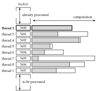
Figure 2: A graphical representation of the parallel search procedure with 8 threads, when processing buckets from index 5690 to index 5697. The bars to the right of the buckets represent the amount of computation that threads have to do before computing the first successful pilot. The shaded part of the bars corresponds to the work done for unsuccessful pilots (those that create collisions in the bitmap). In this example, thread 2 (in bold font) has to commit its work, therefore it can execute until success (the shaded part covers its entire bar). The crucial point is that: the shaded part can be computed in parallel, hence saving time compared to the sequential implementation.

We spawn $K$ parallel threads and work on $K$ consecutive buckets with one thread per bucket. Each thread advances in the search of a pilot independently, pausing the search when a pilot that works for the current state of the bitmap is found. At that point, either the thread is processing the first bucket to commit, or it is waiting for some other thread to update the bitmap. In the former case, the thread (i) concludes the pilot search, (ii) updates the bitmap, and (iii) starts processing the next bucket to be processed. Only one thread at a time can thus update the bitmap. In the latter case, the waiting thread wakes up after a bitmap update and continues the pilot search according to the new state of the bitmap, pausing as soon as it finds a new working pilot.

The crucial point, now, is to manage the turns between the threads in an efficient way. To do so, we label the threads with unique identifiers, from $0$ to $K-1$, and maintain the following invariant: thread $i$ processes the bucket of index $0\leq j<m$ where $i=j\,\textup{mod}{\,K}$ (see Fig. 2 for an example with $K=8$). It follows that the threads must finalize their respective computation and commit changes to the bitmap following the identifier order to guarantee correctness. We guarantee this ordering using a shared identifier, periodically indicating the thread that is allowed to commit. Therefore, a thread advances the search as far as it can by checking (inside a loop, sometimes called “busy waiting”) the shared identifier. If the shared identifier is equal to its own identifier, then the thread can commit its work. Note that we do not require a lock/unlock mechanism to synchronize the threads that would sensibly erode the benefit of parallelism, but rely on the value assumed by the shared identifier. This is a rather important point to obtain good practical performance.

At the beginning of the algorithm, the shared identifier is equal to $0$, hence only the first thread is allowed to conclude the search and update the bitmap. Then, the shared identifier is set to $1$ by the first thread. The second thread can now commit, and so on. In general, the turn of the thread $i$ comes when all threads $0\leq j<i$ have committed. The shared identifier is set back to $0$ when the thread $K-1$ commits.

4.2 Internal Memory

In this setting, we assume that the construction algorithm has enough internal memory available. We have to specify only few details given the flexibility of the algorithm presented in Section 3.

• The blocks output by the map step are materialized as in-memory vectors of pairs. The total space taken is therefore $n(q_{1}+q_{2})$ bytes. Let $K$ be the number of parallel threads to use. The map step spawns $K$ threads. Each thread allocates a vector of $n/K$ pairs and fills it by forming pairs from a partition of $S$ consisting in $n/K$ keys. Once the vector is filled up, it is sorted. Since the threads work on different partitions of $S$, the map with $K$ threads achieves nearly ideal speed-up.

• The collection of buckets output by the merge step consists in $L$ in-memory vectors of hash codes, whose total cost is $(n+m)q_{2}$ bytes. During the merge procedure, the blocks output by the map and the buckets under construction co-exist, hence the total memory usage is $n(q_{1}+q_{2})+(n+m)q_{2}=n(q_{1}+2q_{2})+mq_{2}$ bytes.

  There is no meaningful opportunity for parallelization during the merge step.

• The auxiliary arrays used by the search step, i.e., taken and positions are materialized as in-memory arrays of 64-bit integers. The pilots table $P$ in the pseudocode of Alg. 2 is also implemented with a 64-bit integer array. Since $P$ fits in internal memory, the saving of a pilot in line 21 simplifies to $P[\mbox{\emph{bucket}}.\mbox{\emph{id}}]=k_{i}$ so that $P$ is already sorted and the $\textsc{Sort}(P)$ step in line 24 is not performed at all. The search can be executed in parallel using $K$ threads as we explained in Section 4.1. The total space used for taken is $\lceil\frac{n}{8\alpha}\rceil$ bytes. The space for $P$ is $8m$ bytes. The space for the free array is $(\lceil\frac{n}{\alpha}\rceil-n)8$ bytes instead.

The overall space used by the internal-memory construction is therefore

$$\max\{ n(q_{1}+2q_{2})+mq_{2},$$

$$\lceil n/(8\alpha)\rceil+8m+(\lceil n/\alpha\rceil-n)8+(n+m)q_{2}\}$$

bytes. For example, the space is at most $\max\{20n+8m,16.25n+16m\}$ bytes for $\alpha>1/2$, which is $20n+8m$ bytes unless a very large $c$ is used.

4.3 External Memory

When not enough internal memory is available for the construction, e.g., because the size of $S$ is very large, it is mandatory to resort to external memory. The general algorithm described in Section 3 easily adapts to this scenario because the steps of the algorithm do not change, rather the output of map and merge is written to (resp. read from) disk. Let $M$ indicate the maximum amount of internal memory (in bytes) that the construction is allowed to use, and $q$ be the number of bytes taken by a $\langle\mbox{\emph{id}},\mbox{\emph{hash}}\rangle$ pair.

• During the map step, we allocate an in-memory vector of size $\lceil M/q\rceil$ pairs. Whenever the vector fills up, it is sorted (possibly in parallel) and flushed to a new file on disk, as to guarantee that at most $M$ bytes of internal memory are used during the process.

• Let $K$ be the number of files created during the map step, i.e., $K=\lceil(qn)/M\rceil$. The pairs from these $K$ files are merged together to create the collection of $L$ buffers representing the buckets. Again, the $L$ buffers are formed in internal memory without violating the limit of $M$ bytes. Whenever the limit is reached, the content of the buffers is accumulated to $L$ files on disk.

• The buckets are read from the $L$ files and processed by the search procedure, possibly by its parallel implementation described in Section 4.1.

  We point out that the bitmap taken is always kept in internal memory (and the array positions as well), because its access pattern is random and the search would be slowed down to unacceptable rates if the bitmap were resident on disk. Therefore, since the search needs $N=\lceil n/\alpha\rceil$ bits of internal memory, we are left with $M-\lceil N/8\rceil$ bytes available to store the pilots.

  The pilots are accumulated in an in-memory vector of $\lceil(M-\lceil N/8\rceil)/q\rceil$ pairs $\langle\mbox{\emph{id}},\mbox{\emph{pilot}}\rangle$ (also these pairs consume $q$ bytes each as those used during the map step). Whenever the $M$-byte limit is reached, the vector is flushed to disk and emptied. Lastly, the different files containing the pilots are merged together to obtain the final $P$ table – the $\textsc{Sort}(P)$ step in line 24 of the algorithm in Alg. 2.

5 Experimental Results

For the experimental results in this section, we use a server machine equipped with 8 Intel i9-9900K cores (@3.60 GHz), 64 GB of RAM DDR3 (@2.66 GHz), and running Linux 5 (64 bits). For all experiments where parallelism is enabled we use 8 parallel threads, one thread per core. Each core has two private levels of cache memory: 32 KiB L1 cache (one for instructions and one for data); 256 KiB for L2 cache. A shared L3 cache spans 16 MiB. All cache levels have a line size of 64 bytes. All datasets are read from a Western Digital Red mechanical disk with 4 TB of storage and a rotation rate of 5400 rpm (SATA 3.1, 6 GB/s).

The implementation of PTHash is written in C++ and available at https://github.com/jermp/pthash. We use the C++ std::thread library to support parallel execution, i.e., without relying on other frameworks such as Intel’s TBBs or OpenMP that would otherwise limit the portability of our software. For the experiments reported in the article, the code was compiled with gcc 9.2.1 using the flags: -std=c++17 -pthread -O3 -march=native.

Methodology

Construction time is reported in total seconds (resp., minutes in external memory), taking the average between 3 runs. Lookup time is measured by loading the MPHF data structure in memory and looking up every single key in the input using a single core of the processor. The reported lookup time is the average between 5 runs. For inputs residing on disk, we load batches of 8 GB of keys in internal memory and measure lookup time on each batch. The final reported time is the weighted average among the measurements on all batches. Lookup time is reported in nanoseconds per key (ns/key). The space of the MPHF data structures is reported in bits per key (bits/key).

A testing detail of particular importance is that, before running a construction algorithm, the disk cache is cleared to ensure that the whole input dataset is read from the disk.

TABLE III: String collections used in the experiments.

Collection	num. strings	GBs	avg. str. length
UK2005 URLs	39,459,925	2.9	71.37
ClueWeb09-B URLs	49,937,704	2.8	54.72
GoogleBooks 2-gr	665,752,080	12.1	17.21
TweetsKB IDs	1,983,291,944	39.2	18.75
ClueWeb09-Full URLs	4,780,950,911	326.5	67.28
GoogleBooks 3-gr	7,384,478,110	179.5	23.30

Datasets

We use some real-world string collections as input datasets. Table III reports the basic statistics for these collections. All datasets are publicly available for download by following the corresponding link in the References.

We use natural-language $q$-grams as they are in widespread use in IR, NLP, and Machine-Learning applications. Specifically, we use the 2-3-grams from the English GoogleBooks corpus, version 2 [34], as also used in prior work on the problem [17, 29]. URLs are interesting as they represent a sort of “worst-case” input given their very long average length. We use those of the Web pages in the ClueWeb09 dataset [35] (category B and full dataset), and those collected in 2005 from the UbiCrawler [36] relative to the .uk domain [37]. TweetsKB [38] is a collection of unique tweets identifiers (IDs), corresponding to tweets collected from February 2013 to December 2020.

As TweetsKB IDs, ClueWeb09-Full URLs, and GoogleBooks 3-gr do not fit in the internal memory of our test machine (64 GB), we are going to use these three datasets to benchmark the construction algorithms in external memory. The other three datasets can be processed in internal memory.

TABLE IV: Internal-memory construction time (in seconds), space, and lookup time, for a range of algorithms.
Numbers in parentheses refer to the parallel construction using 8 threads. All PTHash configurations use $\alpha=0.94$ and $c=7.0$.

Algorithm		UK2005 URLs					ClueWeb09-B URLs					GoogleBooks 2-gr
		construction		space	lookup		construction		space	lookup		construction		space	lookup
		(seconds)		(bits/key)	(ns/key)		(seconds)		(bits/key)	(ns/key)		(seconds)		(bits/key)	(ns/key)
PTHash (D-D)		9	(5)	2.82	49		12	(6)	3.07	49		410	(156)	2.97	63
PTHash (PC)				2.82	49				2.80	52				2.67	69
PTHash (EF)				2.50	59				2.49	63				2.38	121
PTHash-HEM (D-D)		8	(2)	3.11	52		10	(2)	3.08	57		167	(34)	2.97	72
PTHash-HEM (PC)				2.82	54				2.80	59				2.67	80
PTHash-HEM (EF)				2.50	66				2.49	70				2.38	159
FCH ($c=3.0$)		1138		3.00	52		1438		3.00	55		–		–	–
FCH ($c=4.0$)		266		4.00	60		267		4.00	64		9110		4.00	54
FCH ($c=5.0$)		119		5.00	68		107		5.00	71		3225		5.00	55
CHD ($\lambda=4$)		32		2.17	170		43		2.17	185		1251		2.17	410
CHD ($\lambda=5$)		84		2.07	173		115		2.07	182		3923		2.07	410
CHD ($\lambda=6$)		306		2.01	173		429		2.01	178		15583		2.01	406
EMPHF		10		2.61	126		13		2.61	135		276		2.61	211
EMPHF-HEM		9		3.49	152		11		3.30	158		148		3.44	287
GOV		39	(14)	2.23	87		47	(15)	2.23	94		613	(170)	2.23	170
BBHash ($\gamma=1.0$)		50	(12)	3.10	154		66	(14)	3.06	174		1248	(189)	3.08	273
BBHash ($\gamma=2.0$)		31	(7)	3.71	133		40	(9)	3.71	150		666	(102)	3.71	204
RecSplit ($\ell=5$, $b=5$)		6		2.95	153		8		2.95	148		132		2.95	244
RecSplit ($\ell=8$, $b=100$)		37		1.79	113		47		1.79	118		724		1.80	202
RecSplit ($\ell=12$, $b=9$)		225		2.23	93		284		2.23	107		3789		2.23	225

Algorithms and Implementations

PTHash is compared against the state-of-the-art algorithms reviewed in Section 2. Table II at page II indicates what implementations support parallel execution and external-memory processing. The “HEM” suffix used in the tables stands for heuristic external memory [16] and refers to the approach of partitioning the input and building an independent MPHF on each partition.

Whenever possible, we used the implementations available from the original authors. We include a link to the source code in the References section. All implementations are in C/C++, except for the construction of GOV which is only available in Java (but lookup time is measured using a C program). Moreover, we also tested the algorithms using the same parameters as suggested by their respective authors to offer different trade-offs between construction time and space effectiveness. Below we report some details.

FCH is the only algorithm that we re-implemented (in C++) faithfully to the original paper. For the CHD algorithm we were unable to use $\lambda=7$ for more than a few thousand keys. The EMPHF library also includes the corresponding HEM implementation of the algorithm, EMPHF-HEM. The authors of BBHash also considers $\gamma=5.0$ in their own work but we obtained a space larger than 6.8 bits/key, so we excluded this value of $\gamma$ from the analysis.

5.1 Internal Memory

Table IV shows the performance of the algorithms on the datasets that can be processed entirely in internal memory. The numbers in parentheses refer to the parallel construction using 8 threads; moreover, all PTHash configurations use $\alpha=0.94$ and $c=7.0$.

Let us first consider the sequential construction and formulate some general observations. PTHash is the fastest MPHF data structure at evaluation time. FCH offers similar lookup performance but PTHash is more space-efficient and much faster at construction time (FCH with $c=3.0$ takes too much time to run over the GoogleBooks 2-gr dataset). Moreover, PTHash offers good space effectiveness, albeit not the best: around 3.2 bits/key using the D-D encoding but less using PC, i.e., around 2.7 – 2.8 bits/key, and even less using Elias-Fano (EF), i.e., around 2.4 – 2.5 bits/key. For algorithms achieving a similar space, such as BBHash, PTHash is 2$\times$ faster at lookup time, and even better at construction time. Compared to more space-efficient algorithms, such as RecSplit or CHD, PTHash is 2 – 6$\times$ faster at lookup time with better construction time.

For the HEM implementation of PTHash we fix the average partition size to $b=5\times 10^{6}$ and let the number of partitions be approximately $n/b$. Therefore, we use 8, 16, and 128 partitions for UK2005 URLs, ClueWeb09-B URLs, and GoogleBooks 2-gr respectively. It is worth noting that PTHash-HEM is faster to build than PTHash, and the gap increases by increasing $n$. For example, building 128 partitions takes 170 seconds on the GoogleBooks 2-gr dataset instead of 410 seconds, hence 2.45$\times$ faster. This is a direct consequence of the complexity of the search that is not linear in $n$ as per Theorem 1. Thus, building $n/b$ functions each for $\approx$$b$ keys is faster than building a single function for $n$ keys.

Another meaningful point to observe is that PTHash-HEM imposes a slight penalty at lookup time compared to PTHash (e.g., around 10 – 16% on most datasets and encoders), with no space overhead. As a comparison, EMPHF-HEM imposes a penalty of 17 – 36% at lookup time and of 26 – 33% of space usage compared to EMPHF. It is desirable that the space of the HEM representation with $r$ partitions is very similar to that of the un-partitioned data structure built from the same input with $m=\lceil cn/\log_{2}(n)\rceil$ buckets. To this end, we search for each MPHF partition using exactly $\lfloor m/r\rfloor$ buckets so to guarantee that the total number of buckets used by the HEM data structure is $m$. In fact, note that using $\lfloor m/r\rfloor$ buckets for the $i$-th partition is different than letting the search over $n_{i}$ keys to use $\lceil cn_{i}/\log_{2}(n_{i})\rceil$ buckets because of the non-linearity of the $\log_{2}$ function. In particular, for an average partition size $n_{i}$ close to $n/r$, $\lfloor m/r\rfloor<\lceil cn_{i}/\log_{2}(n_{i})\rceil$ holds.

We now discuss the results for parallel constructions. Since a parallel construction has the clear advantage of reducing construction time, it can be used to either:

• build functions more quickly, for a fixed space budget;

• build more compact functions by selecting tighter parameters $c$ and $\alpha$ for the search, for a fixed construction-time budget.

The numbers in parentheses in Table IV show that construction time improves significantly. The parallel algorithm reduces construction time by 2 – 2.5$\times$, thus allowing PTHash to build faster than its direct competitors that also exploit multi-threading, like GOV and BBHash. Better speedup can be achieved, not surprisingly, by PTHash-HEM because partitions can be built independently in parallel.

TABLE V: External-memory construction time (in minutes), space, and lookup time, for a range of algorithms.
Numbers in parentheses refer to the parallel construction using 8 threads. All PTHash configurations use $\alpha=0.94$ and $c=7.0$.

Algorithm		TweetsKB IDs					ClueWeb09-Full URLs					GoogleBooks 3-gr
		construction		space	lookup		construction		space	lookup		construction		space	lookup
		(minutes)		(bits/key)	(ns/key)		(minutes)		(bits/key)	(ns/key)		(minutes)		(bits/key)	(ns/key)
PTHash (D-D)		36	(18)	3.07	80		121	(82)	2.96	120		163	(98)	2.91	91
PTHash (PC)				2.61	101				2.58	175				2.56	143
PTHash (EF)				2.36	188				2.32	214				2.31	208
PTHash-HEM (D-D)		17	(10)	2.85	116		78	(61)	2.75	152		87	(59)	2.71	135
PTHash-HEM (PC)				2.61	128				2.58	192				2.57	190
PTHash-HEM (EF)				2.36	201				2.32	235				2.31	230
EMPHF		68		2.61	207		415		2.61	231		629		2.61	220
EMPHF-HEM		16		3.03	279		67		3.31	304		94		3.06	304
GOV		45	(25)	2.23	192		138	(90)	2.23	232		180	(108)	2.23	242
BBHash ($\gamma=1.0$)		80	(16)	3.07	294		323	(307)	3.07	320		337	(160)	3.07	305
BBHash ($\gamma=2.0$)		40	(10)	3.71	217		185	(173)	3.71	236		171	(91)	3.71	235

Fig. 3 highlights, instead, that parallelism can also be used to build more space-efficient functions. In the figure, the horizontal line marks the lowest construction time achieved by sequential PTHash (for $c=7.0$), so that it is easy to see the same time is spent by the parallel PTHash for a smaller $c$. For example, $c$ can be reduced from 7.0 to 5.0 for $\alpha=0.94$ to build a smaller MPHF within the same time-budget using 8 parallel threads. The companion Fig. 4 shows the space consumption and lookup time corresponding to such values of $c$. Continuing the same example, for the D-D encoder, space improves from 2.97 to 2.63 bits/key for $\alpha=0.94$. As another example (not shown in the plots), for $\alpha=0.99$ we obtained a similar space improvement: from 2.89 to 2.52 bits/key.

Fig. 4 also shows that the partitioned compact encoding (PC) introduced in Section 3 is always more effective than D-D with only a minor lookup penalty. PC may be preferable to EF for its better lookup performance despite the latter being still more space-efficient. We report two more illustrative examples:

• Compared to RecSplit $(\ell=12,b=9)$, parallel PTHash with $\alpha=0.99$ and $c=4.0$ builds faster (2710 vs. 3789 seconds) and, using PC, it retains even better space (2.12 vs. 2.23 bits/key), with $3.75\times$ faster lookup time.

• Elias-Fano (EF) allows PTHash to break the 2 bits/key “barrier”, indeed consuming only 1.98 bits/key for $\alpha=0.99$ and $c=4.0$: we point out that, up to date, only RecSplit was able to do so. Using that configuration of parameters, PTHash-HEM is only slightly larger than RecSplit $(\ell=8,b=100)$, i.e., 1.98 vs. 1.80 bits/key, but builds nearly $2\times$ faster with $1.5\times$ better lookup time.

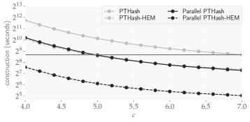
Figure 3: Internal-memory construction time of PTHash and PTHash-HEM on the GoogleBooks 2-gr dataset, by varying $c$, and for $\alpha=0.94$. The parallel construction uses 8 threads. The horizontal line marks the lowest construction time achieved by sequential PTHash, that is for $c=7.0$. Note the log-scale of the y-axis.

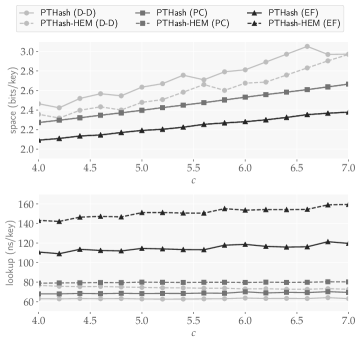
Figure 4: Space/time trade-offs for PTHash and PTHash-HEM by varying $c$ and compressor (D-D, PC, EF), and for $\alpha=0.94$. Performance was measured on the GoogleBooks 2-gr dataset.

5.2 External Memory

Table V shows the performance of the algorithm supporting external-memory processing, on datasets comprising several billions of strings. For PTHash and PTHash-HEM we fixed the amount of internal memory to 16 GB (out of the 64 GB available) as we did not observe any appreciable difference by using less or more memory. The number of partitions used by PTHash-HEM is set using the same methodology of Section 5.1, i.e., we fix the average partition size to $b=5\times 10^{6}$ and let the number of partitions be approximately $n/b$. Therefore, we use 400, 1000, and 1500 partitions for TweetsKB IDs, ClueWeb09-Full URLs, and GoogleBooks 3-gr respectively.

Results for external memory are consistent with those discussed for internal memory: the construction time of PTHash is competitive or better than that of other algorithms, for similar space effectiveness yet better lookup time.

We point out, again, that the parallel search algorithm described in Section 4.1 is a key ingredient to achieve efficient parallel construction, even in external memory. PTHash-HEM offers further reductions in construction time at the cost of a lookup penalty. However, note that the parallel speedup is partially eroded in external memory compared to internal memory, due to I/O operations, even though these are just sequential reads/writes.

Considering Table V, we now illustrate some comparisons using the largest dataset as example, i.e., GoogleBooks 3-gr with approximately 7.4 billion strings, noting that very similar considerations are valid for the other datasets:

• PTHash with D-D is $2\times$ faster than BBHash with $\gamma=1.0$ at construction (163 vs. 337 seconds), retains even better space usage (2.91 vs. 3.07 bits/key), and is $3\times$ faster at lookup time (91 vs. 242 ns/key).

• PTHash with D-D is slightly faster than GOV at construction time with $2.7\times$ faster lookup (91 vs. 242 ns/key), albeit being less space-efficient (2.91 vs. 2.23 bits/key). Instead, PTHash-HEM with EF is as efficient as GOV regarding space and lookup time, but with almost $2\times$ better construction time (87 vs. 180 seconds).

• PTHash with PC is nearly $4\times$ faster at construction than EMPHF (163 vs. 629 seconds), retains the same space and $1.5\times$ better lookup (143 vs. 220 ns/key). The HEM implementation of PTHash outperforms the HEM implementation of EMPHF under every aspect.

6 Conclusions

In this work we described a construction algorithm for PTHash that enables multi-threading and external-memory processing. These two features are very important to scale to large datasets in reasonable time. Our C++ implementation is publicly available at https://github.com/jermp/pthash.

We presented an extensive experimental analysis and comparisons, using large real-world string collections. There are three efficiency aspects for minimum perfect hash data structures: construction time, space consumption, and lookup time. PTHash can be tuned to match the performance of another algorithm on one of the three aspects and, then, outperform the same algorithm on the other two aspects. We remark that lookup time may be the most relevant aspect in concrete applications of minimal perfect hashing. In this regard, PTHash offers very fast evaluation being from $2$ to $6\times$ faster than other competitive techniques.

In this appendix we prove Theorem 1. To do so, we first introduce some technical machinery.

The thresholds $p_{1}=0.6n$ and $p_{2}=0.3m$ introduced in Section 3.1 logically partition the $n$ keys of $S$ into two sets of buckets, $M_{1}$ and $M_{2}$: $M_{1}$ contains $n_{1}=0.6n$ keys and $m_{1}=0.3m$ buckets; $M_{2}$ instead contains $n_{2}=0.4n$ keys and $m_{2}=0.7m$ buckets. The number of keys of the different buckets can be modeled by $m$ random variables. Clearly, the random variables of buckets in $M_{1}$ are independent from those of the buckets in $M_{2}$. Moreover, all random variables belonging to the same set of buckets are distributed in the same way: we indicate with $X_{1}$ the bucket size of the buckets from $M_{1}$ and with $X_{2}$ that of the buckets from $M_{2}$. For $k\in\{1,2\}$, we know that $X_{k}$ is a binomially-distributed random variable – $X_{k}\sim\operatorname{\mathtt{Binomial}}(n_{k},1/m_{k})$ – with expectation $\lambda_{k}=n_{k}/m_{k}$. Let $\lambda=n/m=\log_{2}(n)/c$. Then $\lambda_{1}=2\lambda$ and $\lambda_{2}=(4/7)\lambda$. We also know that $\operatorname{\mathtt{Binomial}}(N,p)$ converges to $\operatorname{\mathtt{Poisson}}(\lambda=Np)$ for $N,1/p\to\infty$. Hence, for $n\to\infty$, we have $X_{k}\sim\operatorname{\mathtt{Poisson}}(\lambda_{k})$ with

$$\operatorname{\mathbb{P}}(X_{k}=t)=\frac{e^{-\lambda_{k}}\lambda_{k}^{t}}{t!}$$ (2)

for $t\in\mathbb{N}\cup\{0\}$ and $k\in\{1,2\}$.

Lemma 1.

Let $\alpha_{\geq t}$ be the load factor after all buckets of size $\geq t$ have been processed. Then, for $n\to\infty$, we have

$$\operatorname{\mathbb{E}}[\alpha_{\geq t}]=\alpha\Big{(}0.6\operatorname{\mathbb{P}}(X_{1}\geq t-1)+0.4\operatorname{\mathbb{P}}(X_{2}\geq t-1)\Big{)}.$$

Proof.

Let $n_{\geq t}$ be the number of keys belonging to buckets of size $\geq t$. Clearly, $\alpha_{\geq t}=\alpha\cdot n_{\geq t}/n$, thus, by linearity of expectation, it suffices to compute $\operatorname{\mathbb{E}}[n_{\geq t}]$ to prove the lemma. We can write $n_{\geq t}$ as

$$n_{\geq t}=\sum_{i=0}^{m_{1}-1}\sum_{j=t}^{n}jI_{1,ij}+\sum_{i=0}^{m_{2}-1}\sum_{j=t}^{n}jI_{2,ij}$$

where

$$I_{k,ij}=\left\{\begin{array}[]{ll}1&\text{bucket }i\text{ from partition }k\text{ contains }j\text{ keys}\\ 0&\text{otherwise}\\ \end{array}\right.$$

for $k\in\{1,2\}$. Now, by linearity of expectation and knowing that $\operatorname{\mathbb{E}}[I_{k,ij}]=\operatorname{\mathbb{P}}(X_{k}=j)$ for any $i$, we have that

$$\operatorname{\mathbb{E}}[n_{\geq t}]=m_{1}\sum_{j=t}^{n}j\operatorname{\mathbb{P}}(X_{1}=j)+m_{2}\sum_{j=t}^{n}j\operatorname{\mathbb{P}}(X_{2}=j).$$

For Equation 2, we have that

$$\sum_{j=t}^{n}j\operatorname{\mathbb{P}}(X_{k}=j)=\sum_{j=t}^{n}j\cdot\frac{e^{-\lambda_{k}}\lambda^{j}_{k}}{j!}=$$

$$\lambda_{k}\sum_{j=t}^{n}\frac{e^{-\lambda_{k}}\lambda^{j-1}_{k}}{(j-1)!}=\lambda_{k}\sum_{j=t-1}^{n-1}\operatorname{\mathbb{P}}(X_{k}=j)=$$

$$\lambda_{k}\operatorname{\mathbb{P}}(X_{k}\geq t-1)$$

for $k\in\{1,2\}$. Replacing the latter equality in the previous expression for $\operatorname{\mathbb{E}}[n_{\geq t}]$, it follows that

$$\operatorname{\mathbb{E}}[n_{\geq t}] =m_{1}\lambda_{1}\operatorname{\mathbb{P}}(X_{1}\geq t-1)+m_{2}\lambda_{2}\operatorname{\mathbb{P}}(X_{2}\geq t-1)$$

$$=0.6n\operatorname{\mathbb{P}}(X_{1}\geq t-1)+0.4n\operatorname{\mathbb{P}}(X_{2}\geq t-1).$$

∎

Lemma 2.

The random variable $\alpha_{\geq t}$ is tightly concentrated around $\operatorname{\mathbb{E}}[\alpha_{\geq t}]$ with high probability.

Proof.

We show the lemma using the McDiarmid’s inequality (which, in turn, is a variation of the Azuma-Hoeffding inequality) [39, Theorem 13.7].

The variable $\alpha_{\geq t}$ is a random variable that depends on the random placement of keys into buckets. Let $Y_{i}$ be the random variable indicating the bucket into which the $i$-th key falls. Clearly, $Y_{1},\ldots,Y_{n}$ are independent random variables. We claim that $\alpha_{\geq t}=f(Y_{1},\ldots,Y_{n})$ satisfies the Lipschitz condition with bound $\frac{\alpha t}{n}$. In fact, the placement of a key in a bucket cannot change the load factor due to buckets of size $\geq t$ by more than $\frac{\alpha t}{n}$ because: (i) if the key is placed in a bucket of size $\leq t-2$, the load factor does not change; (ii) if it falls in a bucket of size $t-1$, the load factor increases by $\frac{\alpha t}{n}$; (iii) lastly, if it falls in a bucket of size $\geq t$, the load factor increases by $\frac{\alpha}{n}$. We can therefore apply the McDiarmid’s inequality to show that

$$\operatorname{\mathbb{P}}(|\alpha_{\geq t}-\operatorname{\mathbb{E}}[\alpha_{\geq t}]|\geq\varepsilon)\leq 2e^{-2n(\frac{\varepsilon}{\alpha t})^{2}},\text{ for }t=1,\ldots,L.$$

The bound above is at most $2e^{-O(n/(\log_{2}(n))^{2})}=O(1/n)$ since $t\leq L=\Theta(\log(n)/c)$. ∎

Lemma 3 (Theorem 5.4 [39]).

Let $X\sim\operatorname{\mathtt{Poisson}}(\lambda)$. We have that $\operatorname{\mathbb{P}}(X\geq t)\leq e^{-\lambda}(\frac{e\lambda}{t})^{t},\text{ for any }t\geq\lambda$.

We are now ready to prove Theorem 1.

Proof of Theorem 1.

As shown by Equation 1, the expected number of trials for the $i$-th bucket is

$$\operatorname{\mathbb{E}}[k_{i}]+1=1/p_{i}=(1-\alpha(i))^{-|B_{i}|}.$$ (1)

Note that, for $|B_{i}|=t$, $(1-\alpha(i))^{-|B_{i}|}\leq(1-\alpha_{\geq t})^{-t}.$ Here, we can use $\operatorname{\mathbb{E}}[\alpha_{\geq t}]$ in place of $\alpha_{\geq t}$ since we know that the error committed will be arbitrarily small with high probability from Lemma 2.

We now separately analyze the large and the small buckets to show an upper bound to the expected number of trials for each bucket. When $t\geq 4\lambda+1$ (large buckets), the expected number of trials is at most $(1-\alpha_{\geq t})^{-t}\leq(1-\alpha(0.6\cdot e^{-2\lambda}(\frac{e2\lambda}{t-1})^{t-1}+0.4\cdot e^{-(4/7)\lambda}(\frac{e4/7\lambda}{t-1})^{t-1}))^{-t}$ for Lemma 3. Note that the latter bound is decreasing in $t$, hence it is at most $(1-\alpha(0.6\cdot e^{-2\lambda}(\frac{e2\lambda}{4\lambda})^{4\lambda}+0.4\cdot e^{-(4/7)\lambda}(\frac{e4/7\lambda}{4\lambda})^{4\lambda}))^{-(4\lambda+1)}<6.$ In this case, the expected number of trials is therefore bounded by a constant. Instead, when $t\leq 4\lambda$ (small buckets), Equation 1 can be upper bounded by $(1-\alpha)^{-4\lambda}$. Therefore, the expected number of trials is at most $n^{-4/c\cdot\log_{2}(1-\alpha)}=n^{\Theta(\alpha/c)}$, for $0<\alpha<1$.

Taking into account that each trial takes $O(|B_{i}|)$ time, the total expected time of Search (Alg. 2) is $\sum_{i=0}^{m-1}O(|B_{i}|)\cdot(\operatorname{\mathbb{E}}[k_{i}]+1)<O(n)\cdot n^{\Theta(\alpha/c)}=O(n^{1+\Theta(\alpha/c)}).$ ∎

Giulio Ermanno Pibiri is assistant professor at Ca’ Foscari University of Venice, Italy. He received a Ph.D. in Computer Science from the University of Pisa in 2019. His research interests involve large-scale indexing, compressed data structures, and algorithms, with applications to Information Retrieval and Computational Biology.

Roberto Trani received a Ph.D. in Computer Science from the University of Pisa, in 2020. He is a postdoctoral researcher at the National Research Council of Italy (ISTI-CNR), within the High Performance Computing Laboratory, and his research interests are machine learning, algorithms, information retrieval, and high performance computing.

References

- [1] D. Belazzougui and G. Navarro, “Alphabet-independent compressed text indexing,” ACM Transactions on Algorithms, vol. 10, no. 4, pp. 1–19, 2014.
- [2] Y. Lu, B. Prabhakar, and F. Bonomi, “Perfect hashing for network applications,” in 2006 IEEE International Symposium on Information Theory. IEEE, 2006, pp. 2774–2778.
- [3] C.-C. Chang and C.-Y. Lin, “Perfect hashing schemes for mining association rules,” The Computer Journal, vol. 48, no. 2, pp. 168–179, 2005.
- [4] D. Belazzougui, P. Boldi, R. Pagh, and S. Vigna, “Fast prefix search in little space, with applications,” in European Symposium on Algorithms. Springer, 2010, pp. 427–438.
- [5] G. E. Pibiri and R. Venturini, “Handling massive N-gram datasets efficiently,” ACM Transactions on Information Systems, vol. 37, no. 2, pp. 25:1–25:41, 2019.
- [6] G. P. Strimel, A. Rastrow, G. Tiwari, A. Piérard, and J. Webb, “Rescore in a Flash: Compact, Cache Efficient Hashing Data Structures for n-Gram Language Models,” in Proceedings of the 21st Annual Conference of the International Speech Communication Association, 2020, pp. 3386–3390.
- [7] G. E. Pibiri, “Sparse and skew hashing of k-mers,” Bioinformatics, vol. 38, no. Supplement_1, pp. i185–i194, 06 2022.
- [8] ——, “On weighted k-mer dictionaries,” Algorithms for Molecular Biology, vol. 18, no. 3, 2023.
- [9] G. E. Pibiri, Y. Shibuya, and A. Limasset, “Locality-preserving minimal perfect hashing of k-mers,” Bioinformatics, vol. 39, no. Supplement_1, p. i534–i543, 06 2023.
- [10] A. Broder and M. Mitzenmacher, “Network applications of bloom filters: A survey,” Internet mathematics, vol. 1, no. 4, pp. 485–509, 2004.
- [11] B. Fan, D. G. Andersen, M. Kaminsky, and M. D. Mitzenmacher, “Cuckoo filter: Practically better than bloom,” in Proceedings of the 10th ACM International on Conference on emerging Networking Experiments and Technologies, 2014, pp. 75–88.
- [12] T. M. Graf and D. Lemire, “Xor filters: Faster and smaller than bloom and cuckoo filters,” Journal of Experimental Algorithmics (JEA), vol. 25, pp. 1–16, 2020.
- [13] M. L. Fredman, J. Komlós, and E. Szemerédi, “Storing a sparse table with o(1) worst case access time,” Journal of the ACM (JACM), vol. 31, no. 3, pp. 538–544, 1984.
- [14] K. Mehlhorn, “On the program size of perfect and universal hash functions,” in 23rd Annual Symposium on Foundations of Computer Science. IEEE, 1982, pp. 170–175.
- [15] G. E. Pibiri and R. Trani, “PTHash: Revisiting FCH Minimal Perfect Hashing,” in Proceedings of the 44th International ACM SIGIR Conference on Research and Development in Information Retrieval, 2021, pp. 1339–1348.
- [16] F. C. Botelho, R. Pagh, and N. Ziviani, “Practical perfect hashing in nearly optimal space,” Information Systems, vol. 38, no. 1, pp. 108–131, 2013.
- [17] D. Belazzougui, P. Boldi, G. Ottaviano, R. Venturini, and S. Vigna, “Cache-oblivious peeling of random hypergraphs,” in 2014 Data Compression Conference. IEEE, 2014, pp. 352–361. [Online]. Available: https://github.com/ot/emphf
- [18] T. Hagerup and T. Tholey, “Efficient minimal perfect hashing in nearly minimal space,” in Annual Symposium on Theoretical Aspects of Computer Science. Springer, 2001, pp. 317–326.
- [19] E. A. Fox, Q. F. Chen, and L. S. Heath, “A faster algorithm for constructing minimal perfect hash functions,” in Proceedings of the 15th annual international ACM SIGIR conference on Research and development in information retrieval, 1992, pp. 266–273.
- [20] D. Belazzougui, F. C. Botelho, and M. Dietzfelbinger, “Hash, displace, and compress,” in European Symposium on Algorithms. Springer, 2009, pp. 682–693. [Online]. Available: https://github.com/bonitao/cmph
- [21] K. Fredriksson and F. Nikitin, “Simple compression code supporting random access and fast string matching,” in International Workshop on Experimental and Efficient Algorithms. Springer, 2007, pp. 203–216.
- [22] B. S. Majewski, N. C. Wormald, G. Havas, and Z. J. Czech, “A family of perfect hashing methods,” The Computer Journal, vol. 39, no. 6, pp. 547–554, 1996.
- [23] B. Chazelle, J. Kilian, R. Rubinfeld, and A. Tal, “The bloomier filter: an efficient data structure for static support lookup tables,” in Proceedings of the fifteenth annual ACM-SIAM symposium on Discrete algorithms. Citeseer, 2004, pp. 30–39.
- [24] M. Dietzfelbinger and S. Walzer, “Dense peelable random uniform hypergraphs,” in 27th Annual European Symposium on Algorithms (ESA), vol. 144, 2019, pp. 38:1–38:16.
- [25] M. Genuzio, G. Ottaviano, and S. Vigna, “Fast scalable construction of (minimal perfect hash) functions,” in International Symposium on Experimental Algorithms. Springer, 2016, pp. 339–352. [Online]. Available: https://github.com/vigna/Sux4J
- [26] ——, “Fast scalable construction of ([compressed] static— minimal perfect hash) functions,” Information and Computation, p. 104517, 2020.
- [27] I. Müller, P. Sanders, R. Schulze, and W. Zhou, “Retrieval and perfect hashing using fingerprinting,” in International Symposium on Experimental Algorithms. Springer, 2014, pp. 138–149.
- [28] G. Jacobson, “Space-efficient static trees and graphs,” in 30th annual symposium on foundations of computer science. IEEE Computer Society, 1989, pp. 549–554.
- [29] A. Limasset, G. Rizk, R. Chikhi, and P. Peterlongo, “Fast and scalable minimal perfect hashing for massive key sets,” in 16th International Symposium on Experimental Algorithms, vol. 11, 2017, pp. 1–11. [Online]. Available: https://github.com/rizkg/BBHash
- [30] E. Esposito, T. M. Graf, and S. Vigna, “Recsplit: Minimal perfect hashing via recursive splitting,” in 2020 Proceedings of the Twenty-Second Workshop on Algorithm Engineering and Experiments (ALENEX). SIAM, 2020, pp. 175–185. [Online]. Available: https://github.com/vigna/sux
- [31] D. Bez, F. Kurpicz, H.-P. Lehmann, and P. Sanders, “High performance construction of RecSplit based minimal perfect hash functions,” arXiv preprint arXiv:2212.09562, 2022.
- [32] R. M. Fano, “On the number of bits required to implement an associative memory,” Memorandum 61, Computer Structures Group, MIT, 1971.
- [33] P. Elias, “Efficient storage and retrieval by content and address of static files,” Journal of the ACM, vol. 21, no. 2, pp. 246–260, 1974.
- [34] “GoogleBooks Corpus, version 2.0, http://storage.googleapis.com/books/ngrams/books/datasetsv2.html,” 2012.
- [35] “The ClueWeb09 Dataset, https://lemurproject.org/clueweb09/webGraph.php,” 2009.
- [36] P. Boldi, B. Codenotti, M. Santini, and S. Vigna, “Ubicrawler: A scalable fully distributed web crawler,” Software: Practice and Experience, vol. 34, no. 8, pp. 711–726, 2004.
- [37] “UK-2005 URLs, http://data.law.di.unimi.it/webdata/uk-2005,” 2005.
- [38] P. Fafalios, V. Iosifidis, E. Ntoutsi, and S. Dietze, “TweetsKB: A public and large-scale rdf corpus of annotated tweets,” in European Semantic Web Conference. Springer, 2018, pp. 177–190. [Online]. Available: https://data.gesis.org/tweetskb
- [39] M. Mitzenmacher and E. Upfal, Probability and Computing: Randomization and Probabilistic Techniques in Algorithms and Data Analysis, 2nd ed. USA: Cambridge University Press, 2017.