ASCNet: Self-supervised Video Representation Learning
with Appearance-Speed Consistency

Abstract

We study self-supervised video representation learning, which is a challenging task due to 1) lack of labels for explicit supervision; 2) unstructured and noisy visual information. Existing methods mainly use contrastive loss with video clips as the instances and learn visual representation by discriminating instances from each other, but they need a careful treatment of negative pairs by either relying on large batch sizes, memory banks, extra modalities or customized mining strategies, which inevitably includes noisy data. In this paper, we observe that the consistency between positive samples is the key to learn robust video representation. Specifically, we propose two tasks to learn appearance and speed consistency, respectively. The appearance consistency task aims to maximize the similarity between two clips of the same video with different playback speeds. The speed consistency task aims to maximize the similarity between two clips with the same playback speed but different appearance information. We show that optimizing the two tasks jointly consistently improves the performance on downstream tasks, e.g., action recognition and video retrieval. Remarkably, for action recognition on the UCF-101 dataset, we achieve 90.8% accuracy without using any extra modalities or negative pairs for unsupervised pretraining, which outperforms the ImageNet supervised pretrained model. Codes and models will be available.

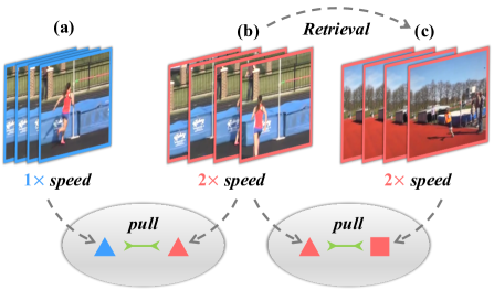
Figure 1: An illustration of appearance-speed consistency. Video clips (a) and (b) come from the same video, and the appearance is consistent with different playback speeds. On the other hand, by using the same frame interval, we can sample the clip (c) from different videos but with the same playback speed as clip (b). We train the model to map clips to appearance and speed embedding space while maintaining the consistency. The appearance-based retrieval strategy reduces the conflict between these two objectives.

1 Introduction

By 2022, almost 79% of the world’s mobile data traffic will be video. With the rise of cameras on smartphones, recording videos has never been easier. Video analysis has become one of the most active research topics [36, 35, 37]. However, the generation of high-quality video data requires a massive human annotation effort (e.g., Kinetics-400 [20], Youtube-8M [1]), which is expensive, time-consuming, and hard to scale up. In contrast, millions of unlabeled videos are freely available on the Internet, e.g., YouTube. Thus, learning meaningful representations from unlabeled videos is crucial for video analysis.

Self-supervised learning makes it possible to exploit a variety of labels that come with the data for free. Instead of collecting manual labels, the proper learning objectives are set to obtain supervision from the unlabeled data themselves. These objectives, also known as pretext tasks, roughly fall into three categories: 1) predicting specific transformations (e.g., rotation angle [19], playback speed [2], and order [39]) of video clips; 2) generative dense prediction, e.g., future frame prediction [13]; and 3) instance discrimination, e.g., CVRL [27] and Pace [34]. Among these methods, the playback speed prediction task has attracted more attention because 1) we can easily train a model with speed labels generated automatically from the video inputs, and 2) models will focus on the moving objects to perceive the playback speed [34]. Thus, models are encouraged to learn representative motion features.

While promising results have been achieved, existing methods suffer from two limitations. First, some of the approaches rely on pre-computed motion information (e.g., optical flow [15, 33]), which is computationally heavy, particularly when the dataset is scaled up. Second, while negative samples play important roles in instance discrimination tasks, it is hard to maintain their quality and quantity. Moreover, same-class negative samples can be harmful [4] to the representations used in downstream tasks.

In this work, we explore the consistency between both appearance and speed of video clips from the same and different instances and eliminate the need for negatives that are detrimental in some cases. To this end, we propose two new pretext tasks, namely, Appearance Consistency Perception (ACP) and Speed Consistency Perception (SCP). Specifically, for the ACP task, we sample two clips from the same video with independent data augmentations and encourage the representations of the two clips to be close enough in feature space. Models cannot finish this task by learning low-level information, i.e., color and rotation. Instead, models tend to learn appearance features such as background scenes and the texture of objects because these features are consistent along a video. For the SCP task, we sample two clips from two different videos with the same playback speed. Representations of these two clips are pulled closer in the feature space. Since the appearance varies from instance to instance, speed can be the crucial clue to finish this task.

Moreover, to enrich the positive samples and integrate the ACP and SCP tasks, we propose an appearance-based video retrieval strategy, which is based on the observation that appearance features in the ACP task achieve a decent accuracy (45% top-1) in the video retrieval task. Thus, we collect the video with the same speed and similar appearance for the SCP task and make it more compatible with the ACP task. This strategy further improves the performance of downstream tasks with negligible computational cost.

To summarize, our contributions are as follows:

• We propose the ACP and SCP tasks for unsupervised video representation learning. In this sense, negative samples no longer affect the quality of learned representations, making the training more robust.

• We propose the appearance-based feature retrieval strategy to select the more effective positive sample for speed consistency perception. In this way, we can bridge the gap between two pretext tasks.

• We verify the effectiveness of our method for learning meaningful video representations on two downstream tasks, namely, action recognition and retrieval, on the UCF-101 [28] and HMDB51 [22] datasets. In all cases, we demonstrate state-of-the-art performance over other self-supervised methods, while our method is easier to apply in practice because we do not have to maintain the collection of negative samples.

2 Related Work

Self-supervised image representation learning. Self-supervised visual representation has recently witnessed tremendous progress on images. A common workflow is to train an encoder on one or multiple pretext tasks with unlabeled images and then use one intermediate feature layer of this model to feed a linear classifier on image classification. The final classification accuracy qualifies how good the learned representation is. The pretext tasks include image rotations [11], jigsaw puzzle [26] and colorization [41]. Recent progress of self-supervised learning is mainly based on instance discrimination, which maintains relative consistency between the representations of the anchor image and its augmented view. The performance of contrastive learning relies on a rich set of negative samples [6, 8, 17]. SimCLR [6] uses a large batch size and picks negatives in a minibatch. MoCo [17] maintains a large dictionary that covers negative features as a memory bank. Nevertheless, same-class negatives are inevitable and harmful to the performance of contrastive learning [4]. Recently, beyond contrastive learning, BYOL [12] and SimSiam [7] learn meaningful representation by only maximizing the similarity between two augmented positive samples without collapsing.

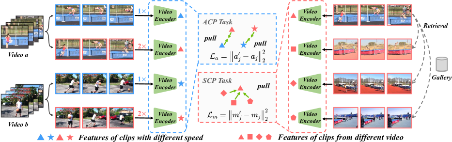
Figure 2: Illustration of the proposed framework. Given a set of video clips with different playback speed (i.e., $1\times$ and $2\times$), we use a video encoder $f(\cdot;\theta)$ to map the clips into appearance and speed embedding space. For the ACP task, we pull the appearance features from the same video closer. For the SCP task, we first retrieve the same speed video with similar contents and then pull the speed features closer. All of the video encoders share the parameters.

Self-supervised video representation learning. In recent years, video analysis has become a popular topic. Unlike static images, videos offer additional opportunities for learning meaningful representation by exploiting spatiotemporal information. Existing methods learn representation through various carefully designed pretext tasks. Some pretext tasks are extended from image-based representation learning, e.g., rotation prediction [19], jigsaw [21]. Other approaches pay more attention to temporal information, including sorting video frames or clips [23]. BE [32] erases the influence of video background by mixing a static frame with the whole clip and removing it. More recently, several attempts have been made through playback speed prediction. SpeedNet [2] predicts whether the video clip is sped up or not, while Pace [34] predicts the exact speed of the video clip. Instead of predicting the absolute playback speed, RSPNet [5] predicts the relative speed to avoid the dependence on imprecise speed labels. However, some movements are too small to make a difference even under different playback speeds. Instead, we only focus on the speed similarity.

3 Approach

Problem definition. We let $\mathcal{V}=\{v_{i}\}_{i=1}^{N}$ be a set of training videos, and we sample a clip $c_{i}$ from $v_{i}$ with playback speed $s_{i}$. Self-supervised video representation learning aims to learn an encoder $f(\cdot;\theta)$ to map the clip $c_{i}$ to consistent feature $\mathbf{x}_{i}$ under different video augmentations.

This task is extremely difficult because of insufficient labels and complex spatiotemporal information. First, it is difficult to construct proper supervision from unlabeled videos for models to learn both appearance and motion information. Second, it is inefficient to capture motion information from video, e.g., by computing optical flow in a sequence of frames. Consequently, the learned representation may not fulfill the requirements of downstream tasks, such as action recognition and video retrieval.

3.1 General Scheme of ASCNet

In this paper, we observe that video playback speed not only is a good source of temporal data augmentation that does not change the spatial appearance but also provides effective supervision for video representation learning. Thus, we propose Appearance Consistency Perception (ACP) task for learning appearance features, i.e., predict consistent appearance features under different spatiotemporal augmentations of the same video, and the Speed Consistency Perception (SCP) task for learning speed features, i.e., predict consistent speed features for different videos with the same playback speed.

Formally, for the ACP task, different from training the model to predict whether or not two clips $c_{i}$ and $c_{j}$ are sampled from the same video, we propose to minimize the distance between the representations of clips $c_{i}$ and $c_{j}$ in the embedding space. Our intuition is that the clips sampled from the same video naturally share similar appearance contents. We also randomize the playback speed so that $s_{i}$ can be equal or not to $s_{j}$. In this way, models are encouraged to learn appearance consistency. For the SCP task, we enforce the models to encode the playback speed information and shorten the distance between the representations of clips $c_{i}$ and $c_{k}$, which are sampled from different videos with $s_{i}=s_{k}$. In this manner, models are encouraged to learn the information that they have in common, namely, the playback speed.

We use two individual projection heads $g_{a}$ and $g_{m}$ to map the representation from $f$ to task corresponding features $\mathbf{a}_{i},\mathbf{a}_{j},\mathbf{m}_{i},\mathbf{m}_{k}$, where $\mathbf{a}_{i},\mathbf{a}_{j}$ are the features for the ACP task and $\mathbf{m}_{i},\mathbf{m}_{k}$ are the features for the SCP task. The overall objective function of our Appearance-Speed Consistency Network (ASCNet) is formulated as follows:

$$\mathcal{L}(\mathcal{V})=\gamma\mathcal{L}_{m}(\mathcal{V})+(1-\gamma)\mathcal{L}_{a}(\mathcal{V}),$$ (1)

where $\mathcal{L}_{a}$ and $\mathcal{L}_{m}$ denote the loss function of the ACP and SCP tasks, respectively. $\gamma$ is a hyperparameter that controls the importance of each task. The pretrained encoder $f(\cdot;\theta)$ and its output feature $\mathbf{x}$ will be used in downstream tasks.

3.2 Appearance Consistency Perception

This task aims to minimize the representation distance between two augmented clips from the same video. Given a video, we sample two clips $c_{i},c_{j}$ with different playback speeds $s_{i},s_{j}$, respectively. We feed the clips into the video encoder $f$ followed by a projection head $g_{a}$ to obtain the corresponding features $\mathbf{a}_{i},\mathbf{a}_{j}$. Following common practice [12, 7], we pass $\mathbf{a}_{i}$ to an additional predictor $h_{a}$ to obtain the prediction $\mathbf{a}_{i}^{\prime}$. We also employ a momentum target encoder, whose parameters $\xi$ is an exponential moving average (EMA) of the corresponding parameters $\theta$. We minimize the feature distance by using $l_{2}$ loss as follows:

$$\mathbf{a}_{i}^{\prime} =h_{a}(g_{a}(f(c_{i};\theta);\theta_{a});\theta_{a}^{\prime})$$ (2)

$$\mathbf{a}_{j} =g_{a}(f(c_{j};\xi);\xi_{a})$$

$$\mathcal{L}_{a} =\left\|\mathbf{a}_{i}^{\prime}-\mathbf{a}_{j}\right\|_{2}^{2}.$$

Since different data augmentations and playback speeds do not change the content of the clip, we expect the appearance features $\mathbf{a}_{i}^{\prime}$ and $\mathbf{a}_{j}$ to be always similar.

3.3 Speed Consistency Perception

Temporal information is crucial for the downstream tasks, e.g., action recognition. Recently, video playback speed prediction has been used as a successful pretext task for perceiving temporal information [2, 34]. However, direct prediction of speed may be suboptimal for learning effective representation because the changes of some motion may be not obvious under different playback speeds. Thus, we propose the consistent speed perception task. This task aims to minimize the distance between two clips with the same playback speed while the appearance can be different. Specifically, we sample two clips $c_{i},c_{k}$ from two videos $v_{i},v_{k}$ in the video set $\mathcal{V}$ with $s_{i}=s_{k}$. Then, these two clips are processed similarly to the ACP task, except that we use projection head $g_{m}$ and predictor $h_{m}$ independent from those in the ACP task. Finally, we define the following $l_{2}$ loss between the prediction and its target feature:

$$\mathbf{m}_{i}^{\prime} =h_{m}(g_{m}(f(c_{i};\theta);\theta_{m});\theta_{m}^{\prime})$$ (3)

$$\mathbf{m}_{k} =g_{m}(f(c_{k};\xi);\xi_{m})$$

$$\mathcal{L}_{m} =\left\|\mathbf{m}_{i}^{\prime}-\mathbf{m}_{k}\right\|_{2}^{2}.$$

However, for two dissimilar videos, the optimization of $\theta$ can be difficult, and it takes more time for the model to converge. Thus, we propose an appearance-based feature retrieval framework to collect similar videos in feature space.

3.3.1 Appearance-based Feature Retrieval

The instance sampling strategy affects the performance of both the SCP and ACP tasks. The clips used in the SCP task can be sampled from the same instance or different instances. However, when using the former, the SCP task may fall back into the ACP task. Since some movements have their corresponding speed, i.e., running and jogging, the latter may lead to conflict between the ACP and SCP tasks. Thus, to reduce the conflict, we propose an appearance-based feature retrieval strategy as follows.

Given an anchor video $v_{i}$, we collect a candidate set of videos (gallery) $\mathcal{C}=\{v_{1},v_{2},...,v_{t}\}_{t=1}^{T}$ from $\mathcal{V}\setminus v_{i}$. We sample a clip from each video to obtain the anchor feature $\mathbf{a}_{i}$ and candidate features $\{\mathbf{a}_{1},\mathbf{a}_{2},...,\mathbf{a}_{t}\}_{t=1}^{T}$ by using the same process as the ACP task. A simple dot product function $d(\cdot,\cdot)$ is used to measure the similarity between the anchor and candidates. Then, we sort the videos by their similarity score and select $v_{k}$ from the most similar candidates. In practice, we use the memory bank [17] to reduce the computation cost. The video pair $v_{i},v_{k}$ can be used in the SCP task with the benefit of strong spatial augmentation while not breaking the appearance consistency.

Algorithm 1 Training method of ASCNet.

0:  Video set $\mathcal{V}=\{v_{i}\}_{i=1}^{N}$, the encoder $f$ with paramaters $\theta$ or $\xi$, the projection heads $g_{a}$ and $g_{m}$ with parameters $\theta_{a}$, $\xi_{a}$, $\theta_{m}$ and $\xi_{m}$, the predictors $h_{a}$ and $h_{m}$ with parameters $\theta_{a}^{\prime}$ and $\theta_{m}^{\prime}$, the hyperparameter $\gamma$.

1:  Randomly initialize parameters $\theta,\theta_{a},\theta_{m},\theta_{a}^{\prime},\theta_{m}^{\prime}$.

2:  Initialize parameters $\xi\leftarrow\theta,\xi_{a}\leftarrow\theta_{a},\xi_{m}\leftarrow\theta_{m}$.

3:  while not convergent do

4:     Randomly sample a video $v$ from $\mathcal{V}$.

5:     Sample two clips $c_{i},c_{j}$ from $v$.

6:     Extract features $\mathbf{x}_{i}{=}f(c_{i},\theta)$, $\mathbf{x}_{j}{=}f(c_{j},\xi)$.

7:     // Learn appearance features with ACP task

8:     Obtain $\mathbf{a}_{i}{=}g_{a}(\mathbf{x}_{i},\theta_{a})$, $\mathbf{a}_{j}{=}g_{a}(\mathbf{x}_{j},\xi_{a})$.

9:     Obtain $\mathbf{a}_{i}^{\prime}=h_{a}(\mathbf{a}_{i},\theta_{a}^{\prime})$.

10:     Compute $\mathcal{L}_{a}=\left\|\mathbf{a}_{i}^{\prime}-\mathbf{a}_{j}\right\|_{2}^{2}$ in Eqn. (2).

11:     // Conduct appearance-based feature retrieval

12:     Construct $\mathcal{C}{=}\{\mathbf{a}_{t}\}_{t=1}^{N-1}$ using $g_{a}(\cdot,\theta_{a})$ from $\mathcal{V}\setminus v$. // Obtain $\mathcal{C}$ efficiently from memory bank

13:     Select the video $\hat{v}$ corresponding to features $\mathbf{a}\in\mathcal{A}$ with the highest dot product similarity with $\mathbf{a}_{j}$.

14:     Sample one clip $c_{k}$ from $\hat{v}$.

15:     Extract features $\mathbf{x}_{k}{=}f(c_{k},\xi)$.

16:     // Learn speed features with SCP task

17:     Obtain $\mathbf{m}_{i}{=}g_{m}(\mathbf{x}_{i},\theta_{m})$, $\mathbf{m}_{k}{=}g_{m}(\mathbf{x}_{k},\xi_{m})$.

18:     Obtain $\mathbf{m}_{i}^{\prime}{=}h_{m}(\mathbf{x}_{i},\theta_{m}^{\prime})$.

19:     Compute $\mathcal{L}_{m}{=}\left\|\mathbf{m}_{i}^{\prime}-\mathbf{m}_{k}\right\|_{2}^{2}$ in Eqn. (3).

20:     Compute $\mathcal{L}=\gamma\mathcal{L}_{m}+(1-\gamma)\mathcal{L}_{a}$ in Eqn (1).

21:     Update parameters $\theta,\theta_{a},\theta_{m},\theta_{a}^{\prime},\theta_{m}^{\prime}$ via SGD.

22:     Compute exponential moving average $\xi,\xi_{a},\xi_{m}$.

23:  end while

4 Experiments

4.1 Datasets

We consider four video datasets, including Mini-Kinetics-200 [38], Kinetics-400 [20], UCF-101 [28], and HMDB-51 [22]. For the self-supervised pretraining, we use the training split of the Kinetics-400 dataset by discarding all of the labels. The Kinetics-400 dataset contains 400 human action categories and provides 240k training video clips and 20k validation video clips. The Mini-Kinetics-200 dataset consists of 200 categories with the most training examples and is a subset of the Kinetics-400 dataset. Since the full Kinetics-400 is quite large, we use Mini-Kinetics-200 to reduce training costs in ablation experiments.

The learned network backbones are evaluated via two downstream tasks: action recognition and nearest neighbor retrieval. For the downstream tasks, UCF-101 [28] and HMDB-51 [22] are used to demonstrate the effectiveness of our method. UCF-101 [28] contains 13k videos spanning over 101 human actions. HMDB-51 [22] contains approximately 7k videos belonging to 51 action classes categories. Both UCF-101 [28] and HMDB-51 [22] come with three predefined training and testing splits. Following prior work [39, 2, 34], we use a training/testing split of 1 for downstream task evaluation. Both datasets exhibit challenges including intraclass variance of actions, cluttered backgrounds, and complex camera motions. Performing action recognition and retrieval on these datasets requires learning rich spatiotemporal representation.

4.2 Implementation Details

Pretraining Settings	Accuracy
w/o pretraining	42.40%
ACP Only	64.76%
SCP Only	43.40%
ASCNet	70.71%

(a) Study on the effectiveness of ASCNet. w/o pretraining denotes training from scratch (random initialization) variants. Backbone: 3D R18.

Method	Configuration	Accuracy
ACP + SP	-	68.93%
ACP + SCP	Same instance	69.20%
ACP + SCP	Different instances	69.55%
ACP + SCP	Similar instances	70.71%

(b) Comparison with different configurations of the SCP task. SP denotes the speed prediction task [2] for each video clip. Backbone: 3D R18.

{$S_{1}$, $S_{2}$}	Accuracy
{$\times$1, $\times$2}	70.71%
{$\times$1, $\times$1}	64.52%
{$\times$1, $\times$4}	70.50%
{$\times$4, $\times$8}	72.16%

(c) Study on different playback speeds set. Backbone: 3D R18.

Batch size	Accuracy
1024	72.20%
512	72.16%
256	72.13%

(d) Study on different batch sizes used in pretraining (200 epochs). Backbone: 3D R18.

Augmentation	Accuracy
Color jittering	62.43%
+ Gaussian blurring	64.55%
+ Random grayscale	67.22%
+ Solarization	72.16%

(e) Ablation on data transformations for pretraining. Backbone: 3D R18.

Backbone	Params	Random	Ours
3D ResNet-18	33.6M	42.40%	72.16%
R(2+1)D	14.4M	56.00%	75.95%
S3D-G	9.6M	45.31%	75.04%

(f) Evaluation of ASC on UCF-101 using different video encoders. We sample 16 frames with 112$\times$112 spatial size for pretraining and fine-tuning.

Table 1: Ablation studies. All models are pretrained with 200 epochs on the Mini-Kinetics-200, except for w/o pretraining setting and evaluation on UCF-101 action recognition by fine-tuning the entire network. Top-1 accuracy is reported.

Backbone networks. To study the effectiveness and generalization ability of our method in detail, we choose three different backbone networks as the video encoder, which have been widely used in recent video self-supervised learning methods, i.e., 3D ResNet [16], R(2+1)D [31], and S3D-G [38]. 3D ResNet [16] is a natural extension of the ResNet architecture [18] for directly tackling 3D volumetric video data by extending 2D convolutional kernels to the 3D counterparts. R(2+1)D [31] is proposed to decompose the full 3D convolution into the 2D spatial convolution followed by the 1D temporal convolution. Moreover, following previous work [2, 34], we use the state-of-the-art backbone S3D-G [38] to further exploit the potential of the proposed approach.

Self-supervised pretraining stage. Following prior work [34, 2, 5], we sample 16 consecutive frames with 112 $\times$112 spatial size for each clip unless specified otherwise. Video clips are augmented using random cropping with resizing, random color jittering, random Gaussian blurring, and random grayscale and solarization. We utilize LARS as the optimizer with a momentum of 0.9 and weight decay of 1e-6 for training without dropout operation. We set the base learning rate to 0.3, scaled linearly with the batch size b; i.e., the learning rate is set to 0.3$\times$b/128. The pretraining process is carried out for 200 epochs by default. The possible playback speed s for the clips in this paper is set to {1$\times$, 2$\times$, 4$\times$, 8$\times$}, i.e., , sampling frames consecutively or setting the sampling interval to {2,4,8} frames. We use only the raw unfiltered RGB video frames as the input and do not make use of optical flow or other auxiliary signals during training. Moreover, we instantiate all projection heads as a fully connected layer with 256 output dimensions. We apply L2 normalization for all features. After pretraining, we drop the projection heads and use the features for downstream tasks. When jointly optimizing $\mathcal{L}_{a}$ and $\mathcal{L}_{m}$, we empirically set the parameters $\gamma$ as 0.5 for loss balance.

Supervised fine-tuning stage. Regarding the action recognition task, during the fine-tuning stage, the learning rate was decayed by a factor of 0.01 over the course of training using cosine annealing. The weights of convolutional layers are retained from the learned representation model, while the weights of the newly appended fully connected layers are randomly initialized. The whole network is then trained with cross-entropy loss.

Evaluation. During inference, following the common evaluation protocol, we sample 10 clips uniformly from each video in the test sets of UCF-101 and HMDB-51. For each clip, we only simply apply the center-crop instead of the ten-crop. Finally, we average the softmax probabilities of all clips as the final prediction.

4.3 Ablation Studies

As shown in Table 1, we provide ablation studies on the effectiveness of the different aspects of our method by self-supervised learning on Mini-Kinetics-200. The representations are evaluated on UCF-101 with end-to-end fine-tuning. The analysis was carried out as follows.

Effectiveness of ASC. In this paper, we propose two tasks to learn effective video representation, namely, Appearance Consistency Perception (ACP) and Speed Consistency Perception (SCP). To verify the effectiveness of our method, we pretrain these models with 3D ResNet-18. As shown in Table 1(a), compared with training from scratch, pretraining with only the ACP task can significantly improve the action recognition performance (64.76% vs. 42.40%) on the UCF-101 dataset, while consistent speed perception further improves the performance from 64.76% to 70.71%, indicating the effectiveness of cooperative work of these two tasks. In the following ablation experiments, unless stated otherwise, we apply 3D ResNet-18 (3D R18) as the backbone.

Ablation on SCP tasks. Here, we instantiate some variants of our method by using different speed perception tasks [2]. SP denotes speed prediction for each individual clip. Table 1(b) shows that the speed consistency perception task improves the performance compared with directly predicting the playback speed of each clip (70.71% vs. 68.93%). Then, we investigate the instance sampling strategy for the SCP task. The video clips used in the SCP task can be sampled from the same instance or different instances. Similar instances denotes using the appearance-based feature retrieval strategy. These results demonstrate that the appearance-based feature retrieval strategy can benefit the speed consistency perception task while not breaking the appearance consistency.

Different playback speed. We denote the $s_{i}$, $s_{j}$ in Algorithm 1 as {$S_{1}$, $S_{2}$}. As shown in Table 1(c), we compare the performance of different playback speed sets {$S_{1}$, $S_{2}$} for our method. In particular, when the speed set is {$\times$1, $\times$1}, our ASC loses the speed perception and degenerates to pay more attention to learning appearance information. As expected, the performance decreases from 70.71% of {$\times$1, $\times$2} to 64.52%, which is similar to the 64.76% of ACP Only in Table 1(a). Then, when the playback speed $S_{1}$ is set to $\times$1, we observe that the changes in $S_{2}$ = $\times$2, $\times$4 appear to have little impact on performance. Interestingly, for {$\times$4, $\times$8}, larger sampling intervals encourage the model to explore longer motion information, boosting the learned representation (70.71% vs. 72.16%). Thus, we adopt it in the following experiments.

Impact of batch size. The ablation study of different batch sizes is shown in Table 1(d). When the batch size changes, we use the same linear scaling rule for all batch sizes studied. Our method works reasonably well over the wide range of batch sizes without using negative pairs. Our experimental results show that a batch size of 256 already achieves high performance. The performance remains stable over a range of batch sizes from 256 to 1024, and the differences are at the level of random variations.

Method	Date	Dataset (duration)	Backbone	Frames	Res.	Single-Mod	UCF	HMDB
Shuffle&Learn [25]	2016	UCF (1d)	CaffeNet	-	224	✓	50.2	18.1
OPN [23]	2017	UCF (1d)	CaffeNet	-	224	✓	56.3	22.1
CMC [30]	2019	UCF (1d)	CaffeNet	-	224	✓	59.1	26.7
MAS [33]	2019	UCF (1d)	C3D	16	112	✗	58.8	32.6
VCP [24]	2020	UCF (1d)	C3D	16	112	✓	68.5	32.5
ClipOrder [39]	2019	UCF (1d)	R(2+1)D	16	$112$	✓	72.4	30.9
PRP [40]	2020	UCF (1d)	R(2+1)D	16	112	✓	72.1	35.0
PSP [9]	2020	UCF (1d)	R(2+1)D	16	112	✓	74.8	36.8
MAS [33]	2019	K400 (28d)	C3D	16	112	✗	61.2	33.4
3D-RotNet [19]	2018	K400 (28d)	3D R18	16	$112$	✓	62.9	33.7
ST-Puzzle [21]	2019	K400 (28d)	3D R18	48	$224$	✓	65.8	33.7
DPC [13]	2019	K400 (28d)	3D R18	64	$128$	✓	68.2	34.5
CBT [29]	2019	K600+ (273d)	S3D-G	-	$112$	✓	79.5	44.6
SpeedNet [2]	2020	K400 (28d)	S3D-G	64	$224$	✓	81.1	48.8
Pace [34]	2020	K400 (28d)	S3D-G	64	224	✓	87.1	52.6
CoCLR-RGB [15]	2020	K400 (28d)	S3D-G	32	$128$	✗	87.9	54.6
RSPNet [5]	2021	K400 (28d)	S3D-G	64	224	✓	89.9	59.6
Ours		K400 (28d)	3D R18	16	$112$	✓	80.5	52.3
Ours		K400 (28d)	S3D-G	64	$224$	✓	90.8	60.5
Fully Supervised [16]		K400 (28d)	3D R18	16	$112$	✓	84.4	56.4
Fully Supervised [38]		ImageNet	S3D-G	64	$224$	✓	86.6	57.7
Fully Supervised [38]		K400 (28d)	S3D-G	64	$224$	✓	96.8	75.9

Table 2: Comparison with state-of-the-art self-supervised learning methods on the UCF-101 and HMDB-51 datasets. The dataset parentheses show the total video duration (d for day, y for year). Single-Mod denotes the Single RGB Modality. K400 represents Kinetics-400.

Arch.	Res.	#Frames	Crop Type	Top-1
S3D-G	224	64	Center-crop	90.77%
	224	64	Three-crop	90.88%
	128	32	Ten-crop	87.31%
3D R18	112	16	Center-crop	80.52%
	112	16	Three-crop	80.73%
	128	16	Three-crop	80.99%

Table 3: Performance of different evaluation protocols. The models are pretrained with 200 epochs on Kinetics-400.

Epochs	100	200	300	400
Top-1 (%)	76.34	80.52	81.31	81.50

Table 4: Performance of different pretraining epochs. A 3D ResNet-18 backbone with ASC pretraining is used.

Augmentation. The accuracies for applying the following data augmentations during pretraining one-by-one are shown in Table 1(e). With only color jittering, our ASC yields 62.43% accuracy. Then, we randomly blur the frames using a Gaussian distribution, boosting the accuracy by 2.1%. Random grayscale is the augmentation approach that converts the frames to grayscale with probability $p$ (default 0.2 in this paper). Equipped with random grayscale, the accuracy of ASC is improved from 64.55% to 67.22%. Finally, we solarize RGB/grayscale video frames by inverting all of the pixel values above a threshold, further improving the performance of our ASC to 72.16%. Overall, by stacking these augmentations, we have steadily improved the learned representation model from 62.42% to 72.16%. Thus, all these data transformations are used in our experiments.

Different backbone. Since it is a general framework, ASC can be widely applied to existing video backbones with consistent gains in performance. In Table 1(f), we compare various instantiations of our framework and show that our method is simple yet effective. We observe a consistent improvement of between 20% and 30% on UCF-101 with our ASCNet on three video decoders, i.e., 3D ResNet-18 [16], R(2+1)D [31], and S3D-G [38].

4.4 Evaluation on the Action Recognition Task

Method	Architecture	Top-$k$
		$k=1$	$k=5$	$k=10$	$k=20$	$k=50$
OPN [23]	CaffeNet	19.9	28.7	34.0	40.6	51.6
Buchler et al.  [3]	CaffeNet	25.7	36.2	42.2	49.2	59.5
ClipOrder [39]	3D R18	14.1	30.3	40.0	51.1	66.5
SpeedNet [2]	S3D-G	13.0	28.1	37.5	49.5	65.0
VCP [24]	3D R18	18.6	33.6	42.5	53.5	68.1
	R(2+1)D	19.9	33.7	42.0	50.5	64.4
Pace [34]	3D R18	23.8	38.1	46.4	56.6	69.8
	C3D	31.9	49.7	59.2	68.9	80.2
RSPNet [5]	C3D	36.0	56.7	66.5	76.3	87.7
	3D R18	41.1	59.4	68.4	77.8	88.7
Ours	3D R18	58.9	76.3	82.2	87.5	93.4

Table 5: Comparison with state-of-the art methods for nearest neighbor retrieval task on the UCF-101 dataset as measured by the top-$k$ retrieval accuracy (%).

Different evaluation protocols. We survey existing self-supervised video representation learning methods and make the following observations about the evaluation protocols: (1) Different works may use different cropping strategies for evaluation, such as center-crop [2, 34, 5], three-crop [27], and ten-crop [13, 14, 15]. (2) Even with the same backbone, many methods may use different resolutions (i.e., $112^{2}$, $128^{2}$, $224^{2}$, $256^{2}$) or numbers of frames (i.e., 16, 32, 64) during evaluation. For readers’ reference, in Table 3, we present the results of our method with different evaluation protocols used in prior works.

Impact of the pretraining epochs. We experiment with pretraining epochs varying from 100 to 400 and report the top-1 accuracy on UCF-101. Table 4 shows the impact of the number of training epochs on performance. While ASC benefits from longer training, it already achieves strong performance after 200 epochs, i.e., 80.52%. We also notice that performance starts to saturate after 300 epochs.

Comparison with the state of the art. In Table 2, we perform a thorough comparison with the state-of-the-art self-supervised learning methods and report the top-1 accuracy on UCF-101 [28] and HMDB-51 [22]. We show the pretraining settings for all approaches, e.g., , pretraining dataset, backbone, number of input frames, resolution, and whether or not only the RGB modality is used. Here, we mainly list the models using RGB as inputs for fair comparisons. Since prior works use different backbones for experiments, we provide results of our ASCNet trained with two common architecture, i.e., 3D ResNet-18 [16], S3D-G [38].

Our ASCNet achieves state-of-the-art results on both the UCF-101 and HMDB-51 datasets. Specifically, when pretrained with the 3D ResNet-18 backbone, our method outperforms 3D-RotNet [19], ST-Puzzle [21], and DPC [13] by a large margin (80.5% vs. 62.9%, 65.8%, and 68.2%, respectively, on UCF-101 and 52.3% vs. 33.7%, 33.7%, and 34.5%). When utilizing S3D-G as the backbone, our ASCNet achieves better accuracy than SpeedNet [2], Pace [34], and RSPNet [5] (90.8% vs. 81.1%, 87.1%, and 89.9%, respectively, on UCF-101 and 60.5% vs. 48.8%, 52.6%, and 59.9%) under the same settings. Remarkably, without the need of any annotation for pretraining, our ASCNet outperforms the ImageNet [10] supervised pretrained model over two datasets (90.8% vs. 86.6%, 60.5% vs. 57.7%).

4.5 Evaluation on the Video Retrieval Task

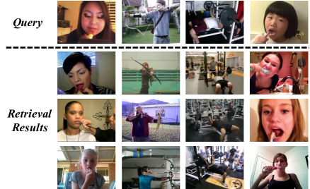
Figure 3: Qualitative examples of the video retrieval task.

Comparison with the state of the art. To further verify the effectiveness of ASCNet, we evaluate our representation with nearest neighbor video retrieval. Specifically, following prior works [34, 2], we uniformly sample 10 clips for each video. For all clips, features are extracted from the video encoder, which is only pretrained with self-supervised learning, and no further fine-tuning is allowed. Then, we perform average-pooling over 10 clips to obtain a video-level feature vector. We use each clip in the test set to query the k nearest clips in the training set. Experiments are conducted on the UCF-101 dataset and we evaluate our method on the split 1 of UCF-101 dataset and apply the top-k accuracies (k = 1, 5, 10, 20, 50) as the evaluation metrics. As shown in Table 5, with the same 3D ResNet-18 backbone, our ASCNet outperforms the state-of-the-art method equivalent on all of the metrics by substantial margins (10.7% - 45.9% for top-1 accuracy on UCF-101). These results indicate that the proposed pretext tasks help us to learn more discriminative features.

Qualitative results for video retrieval. We further provide some retrieval results as a qualitative study. In Figure 3, the top is the query video from the UCF-101 testing set, and the bottom shows the top-3 nearest neighbors from the UCF-101 training set. We successfully retrieve highly relevant videos with similar appearance and motion. This result implies that our method is able to learn both meaningful appearance and motion features for videos.

5 Conclusion

This work presents an unsupervised video representation learning framework named ASCNet, which leverages the appearance consistency throughout the frames of the same video and speed consistency between videos with the same fps. We train the model to map these clips to appearance and speed embedding space while maintaining consistency. We also propose an appearance-based retrieval strategy to reduce the conflict between the appearance and speed consistency perception tasks. Extensive experiments show that the features learned by ASCNet perform better on action recognition and video retrieval tasks. In the future, we plan to incorporate additional modalities into our framework.

Acknowledgments.

This work was partially supported by National Natural Science Foundation of China (NSFC) 62072190, Ministry of Science and Technology Foundation Project (2020AAA0106901), Program for Guangdong Introducing Innovative and Entrepreneurial Teams 2017ZT07X183, CCF-Baidu Open Fund (CCF-BAIDU OF2020022).

References

- [1] Sami Abu-El-Haija, Nisarg Kothari, Joonseok Lee, Paul Natsev, George Toderici, Balakrishnan Varadarajan, and Sudheendra Vijayanarasimhan. Youtube-8m: A large-scale video classification benchmark. arXiv preprint arXiv:1609.08675, 2016.
- [2] Sagie Benaim, Ariel Ephrat, Oran Lang, Inbar Mosseri, William T. Freeman, Michael Rubinstein, Michal Irani, and Tali Dekel. Speednet: Learning the speediness in videos. In CVPR, pages 9919–9928, 2020.
- [3] Uta Büchler, Biagio Brattoli, and Björn Ommer. Improving spatiotemporal self-supervision by deep reinforcement learning. In ECCV, pages 797–814, 2018.
- [4] Tiffany Tianhui Cai, Jonathan Frankle, David J. Schwab, and Ari S. Morcos. Are all negatives created equal in contrastive instance discrimination? arXiv preprint arXiv:2010.06682, 2020.
- [5] Peihao Chen, Deng Huang, Dongliang He, Xiang Long, Runhao Zeng, Shilei Wen, Mingkui Tan, and Chuang Gan. RSPNet: Relative speed perception for unsupervised video representation learning. In AAAI, pages 1045–1053, 2021.
- [6] Ting Chen, Simon Kornblith, Mohammad Norouzi, and Geoffrey E. Hinton. A simple framework for contrastive learning of visual representations. In ICML, pages 1597–1607, 2020.
- [7] Xinlei Chen and Kaiming He. Exploring simple siamese representation learning. arXiv preprint arXiv:2011.10566, 2020.
- [8] Yaofo Chen, Yong Guo, Qi Chen, Minli Li, Yaowei Wang, Wei Zeng, and Mingkui Tan. Contrastive neural architecture search with neural architecture comparators. In The IEEE Conference on Computer Vision and Pattern Recognition, 2021.
- [9] Hyeon Cho, Taehoon Kim, Hyung Jin Chang, and Wonjun Hwang. Self-supervised spatio-temporal representation learning using variable playback speed prediction. arXiv preprint arXiv:2003.02692, 2020.
- [10] Jia Deng, Wei Dong, Richard Socher, Li-Jia Li, Kai Li, and Li Fei-Fei. Imagenet: A large-scale hierarchical image database. In CVPR, pages 248–255. Ieee, 2009.
- [11] Spyros Gidaris, Praveer Singh, and Nikos Komodakis. Unsupervised representation learning by predicting image rotations. In ICLR, 2018.
- [12] Jean-Bastien Grill, Florian Strub, Florent Altché, Corentin Tallec, Pierre H. Richemond, Elena Buchatskaya, Carl Doersch, Bernardo Ávila Pires, Zhaohan Guo, Mohammad Gheshlaghi Azar, Bilal Piot, Koray Kavukcuoglu, Rémi Munos, and Michal Valko. Bootstrap your own latent - A new approach to self-supervised learning. In NeurIPS, 2020.
- [13] Tengda Han, Weidi Xie, and Andrew Zisserman. Video representation learning by dense predictive coding. In ICCVW, pages 1483–1492, 2019.
- [14] Tengda Han, Weidi Xie, and Andrew Zisserman. Memory-augmented dense predictive coding for video representation learning. In ECCV, pages 312–329, 2020.
- [15] Tengda Han, Weidi Xie, and Andrew Zisserman. Self-supervised co-training for video representation learning. In NeurIPS, 2020.
- [16] Kensho Hara, Hirokatsu Kataoka, and Yutaka Satoh. Can spatiotemporal 3d cnns retrace the history of 2d cnns and imagenet? In CVPR, pages 6546–6555, 2018.
- [17] Kaiming He, Haoqi Fan, Yuxin Wu, Saining Xie, and Ross B. Girshick. Momentum contrast for unsupervised visual representation learning. In CVPR, pages 9726–9735, 2020.
- [18] Kaiming He, Xiangyu Zhang, Shaoqing Ren, and Jian Sun. Deep residual learning for image recognition. In CVPR, pages 770–778, 2016.
- [19] Longlong Jing, Xiaodong Yang, Jingen Liu, and Yingli Tian. Self-supervised spatiotemporal feature learning via video rotation prediction. arXiv preprint arXiv:1811.11387, 2018.
- [20] Will Kay, João Carreira, Karen Simonyan, Brian Zhang, Chloe Hillier, Sudheendra Vijayanarasimhan, Fabio Viola, Tim Green, Trevor Back, Paul Natsev, Mustafa Suleyman, and Andrew Zisserman. The kinetics human action video dataset. arXiv preprint arXiv:1705.06950, 2017.
- [21] Dahun Kim, Donghyeon Cho, and In So Kweon. Self-supervised video representation learning with space-time cubic puzzles. In AAAI, pages 8545–8552, 2019.
- [22] Hildegard Kuehne, Hueihan Jhuang, Estíbaliz Garrote, Tomaso A. Poggio, and Thomas Serre. HMDB: A large video database for human motion recognition. In ICCV, pages 2556–2563, 2011.
- [23] Hsin-Ying Lee, Jia-Bin Huang, Maneesh Singh, and Ming-Hsuan Yang. Unsupervised representation learning by sorting sequences. In ICCV, pages 667–676, 2017.
- [24] Dezhao Luo, Chang Liu, Yu Zhou, Dongbao Yang, Can Ma, Qixiang Ye, and Weiping Wang. Video cloze procedure for self-supervised spatio-temporal learning. In AAAI, pages 11701–11708, 2020.
- [25] Ishan Misra, C. Lawrence Zitnick, and Martial Hebert. Shuffle and learn: Unsupervised learning using temporal order verification. In ECCV, pages 527–544, 2016.
- [26] Mehdi Noroozi and Paolo Favaro. Unsupervised learning of visual representations by solving jigsaw puzzles. In ECCV, pages 69–84, 2016.
- [27] Rui Qian, Tianjian Meng, Boqing Gong, Ming-Hsuan Yang, Huisheng Wang, Serge J. Belongie, and Yin Cui. Spatiotemporal contrastive video representation learning. arXiv preprint arXiv:2008.03800, 2020.
- [28] Khurram Soomro, Amir Roshan Zamir, and Mubarak Shah. UCF101: A dataset of 101 human actions classes from videos in the wild. arXiv preprint arXiv:1212.0402, 2012.
- [29] Chen Sun, Fabien Baradel, Kevin Murphy, and Cordelia Schmid. Learning video representations using contrastive bidirectional transformer. arXiv preprint arXiv:1906.05743, 2019.
- [30] Yonglong Tian, Dilip Krishnan, and Phillip Isola. Contrastive multiview coding. In ECCV, pages 776–794, 2020.
- [31] Du Tran, Heng Wang, Lorenzo Torresani, Jamie Ray, Yann LeCun, and Manohar Paluri. A closer look at spatiotemporal convolutions for action recognition. In CVPR, pages 6450–6459, 2018.
- [32] Jinpeng Wang, Yuting Gao, Ke Li, Yiqi Lin, Andy J. Ma, and Xing Sun. Removing the background by adding the background: Towards background robust self-supervised video representation learning. arXiv preprint arXiv:2009.05769, 2020.
- [33] Jiangliu Wang, Jianbo Jiao, Linchao Bao, Shengfeng He, Yunhui Liu, and Wei Liu. Self-supervised spatio-temporal representation learning for videos by predicting motion and appearance statistics. In CVPR, pages 4006–4015, 2019.
- [34] Jiangliu Wang, Jianbo Jiao, and Yun-Hui Liu. Self-supervised video representation learning by pace prediction. In ECCV, pages 504–521, 2020.
- [35] Wenhao Wu, Dongliang He, Tianwei Lin, Fu Li, Chuang Gan, and Errui Ding. Mvfnet: Multi-view fusion network for efficient video recognition. In AAAI, pages 2943–2951, 2021.
- [36] Wenhao Wu, Dongliang He, Xiao Tan, Shifeng Chen, and Shilei Wen. Multi-agent reinforcement learning based frame sampling for effective untrimmed video recognition. In ICCV, pages 6222–6231, 2019.
- [37] Wenhao Wu, Yuxiang Zhao, Yanwu Xu, Xiao Tan, Dongliang He, Zhikang Zou, Jin Ye, Yingying Li, Mingde Yao, Zichao Dong, and Yifeng Shi. Dsanet: Dynamic segment aggregation network for video-level representation learning. In ACMMM, 2021.
- [38] Saining Xie, Chen Sun, Jonathan Huang, Zhuowen Tu, and Kevin Murphy. Rethinking spatiotemporal feature learning: Speed-accuracy trade-offs in video classification. In ECCV, pages 318–335, 2018.
- [39] Dejing Xu, Jun Xiao, Zhou Zhao, Jian Shao, Di Xie, and Yueting Zhuang. Self-supervised spatiotemporal learning via video clip order prediction. In CVPR, pages 10334–10343, 2019.
- [40] Yuan Yao, Chang Liu, Dezhao Luo, Yu Zhou, and Qixiang Ye. Video playback rate perception for self-supervised spatio-temporal representation learning. In CVPR, pages 6547–6556, 2020.
- [41] Richard Zhang, Phillip Isola, and Alexei A. Efros. Colorful image colorization. In ECCV, pages 649–666, 2016.