Bi-Granularity Contrastive Learning for Post-Training in Few-Shot Scene

Abstract

The major paradigm of applying a pre-trained language model to downstream tasks is to fine-tune it on labeled task data, which often suffers instability and low performance when the labeled examples are scarce. One way to alleviate this problem is to apply post-training on unlabeled task data before fine-tuning, adapting the pre-trained model to target domains by contrastive learning that considers either token-level or sequence-level similarity. Inspired by the success of sequence masking, we argue that both token-level and sequence-level similarities can be captured with a pair of masked sequences. Therefore, we propose complementary random masking (CRM) to generate a pair of masked sequences from an input sequence for sequence-level contrastive learning and then develop contrastive masked language modeling (CMLM) for post-training to integrate both token-level and sequence-level contrastive learnings. Empirical results show that CMLM surpasses several recent post-training methods in few-shot settings without the need for data augmentation.

1 Introduction

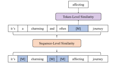
Figure 1: Demonstration of token-level similarity and sequence-level similarity, where the token “affecting” is close to the token “[MASK]” due to the latter’s context. The two sequences with different maskings are also close due to their semantic affinity.

The past few years have seen the rapid proliferation of large-scale pre-trained language models such as GPT Radford et al. (2018), BERT Devlin et al. (2019) and RoBERTa Liu et al. (2019b). These models are generally characterized by pre-training on huge general-domain corpora and then fine-tuning on task-specific labeled examples when applied to a downstream task. Despite tremendous knowledge obtained from general-domain corpora through pre-training, sufficient labeled examples from the task domain are still needed. However, collecting them is often infeasible in many scenes, where it tends to be unstable and low-performing when directly fine-tuning these pre-trained models Zhang et al. (2021); Dodge et al. (2020).

Many efforts have been devoted to addressing the above issue. Firstly, it can be relieved by improving the fine-tuning process, such as introducing regularization Jiang et al. (2020); Lee et al. (2020), re-initializing top layers Zhang et al. (2021), and using debiased Adam optimizer Mosbach et al. (2021). Besides, according to empirical results Zhang et al. (2021); Mosbach et al. (2021), fine-tuning with a small learning rate and more fine-tuning epochs can also improve the situation. Secondly, additional data can be explored, for which two main genres of data might be helpful: labeled examples from related tasks and unlabeled task examples. The former has shown considerable success on the GLUE tasks Phang et al. (2018); Liu et al. (2019a), whereas such labeled examples are not always easy to collect. By contrast, the latter is more feasible, especially in scenes where task examples are easy to collect but expensive to label.

Contrastive learning Hadsell et al. (2006) is a recently re-emerged method for leveraging unlabeled data to enhance representation learning. The key to contrastive learning is to capture the similarity between samples. As shown in Figure 1, there are two sorts of similarities that can be captured for a natural language sequence: token-level similarity and sequence-level similarity. Masked language model (MLM) Devlin et al. (2019), widely adopted in pre-trained language models, can be considered as token-level contrastive learning, as it maximizes the similarity between the “[MASK]” token and the original token before masking and minimizes the similarity with other tokens. As for sequence-level similarity, several works Iter et al. (2020); Giorgi et al. (2020); Wu et al. (2020) introduce sequence-level contrastive learning into pre-training. While all these works focus on the pre-training phase, the focal point of this paper is to improve the performance of pre-trained models in downstream tasks through post-training especially for scenes where limited labeled data is available.

Speaking of pre-trained language models, Xu et al. (2019) and Gururangan et al. (2020) demonstrate improvement in various downstream tasks by training the models with MLM on task examples before fine-tuning, which, following Xu et al. (2019), is termed post-training in this paper even though Gururangan et al. (2020) term it adaptive pre-training. Fang and Xie (2020) also post-train their model on task examples by contrastive self-supervised learning Chen et al. (2020), which pulls together two augmented sentences generated from the same sentence by back-translation Edunov et al. (2018) while separating those otherwise. However, these works consider either token-level or sequence-level contrastive learning, without integrating them. Moreover, adopting back-translation to generate augmented sentences demands considerable computation and makes the effect of post-training dependent on the translation systems.

To capture both sequence-level and token-level similarities, we propose contrastive masked language modeling (CMLM) to achieve more effective knowledge transfer in post-training and to improve the performance of pre-trained language models in few-shot downstream tasks. For this purpose, we propose complementary random masking (CRM) to generate a pair of masked sequences from a single sequence for both sequence-level and token-level contrastive learnings. We conduct extensive experiments to compare CMLM with several recent post-training approaches, and the empirical results show that CMLM achieves superior or competitive performance in a wide range of downstream tasks.

Our contributions can be concluded as follows. First, we propose a new random masking strategy, CRM, to generate a pair of masked sequences favorable to sentence-level contrastive learning. Second, we propose a novel objective, CMLM, for post-training pre-trained language models, which realizes both sequence-level and token-level contrastive learnings on a pair of masked sequences. Third, we compare our approach with several post-training methods and obtain superior or competitive results in few-shot settings. Lastly, we compare two contrastive learning implementations, SimCLR Chen et al. (2020) and SimSiam Chen and He (2020), in pre-trained language models. To our best knowledge, our work is the first effort to implement SimSiam in NLP and compare it with SimCLR.

2 Related Works

2.1 Pre-trained Language Model

Pre-trained language models such as GPT Radford et al. (2018), BERT Devlin et al. (2019) and RoBERTa Liu et al. (2019b) have become a new paradigm of NLP research, and been successfully applied in a wide range of tasks that used to be thorny. These models are generally structured with stacks of Transformer Vaswani et al. (2017) and pre-trained on large-scale unlabeled corpora. Among them, GPT is pre-trained with a unidirectional language modeling objective, and BERT is with masked language modeling (MLM) and next sentence prediction (NSP). In RoBERTa, Liu et al. (2019b) turn the static MLM in BERT into a dynamic one and remove the NSP task, and pre-train it more intensively with larger corpora.

Despite tremendous knowledge learned from unlabeled corpora during pre-training, sufficient labeled task examples are still needed for fine-tuning, which can be challenging for some scenes. Plus, unlabeled task examples are not leveraged when sticking to the pre-training and fine-tuning paradigm.

2.2 Contrastive Learning

To take advantage of unlabeled or labeled data more effectively, contrastive learning Hadsell et al. (2006) is re-emerged recently in computer vision (CV) and natural language processing (NLP). The key to contrastive learning is to pull positive samples together while separating negative samples apart. The construction of positive and negative sample pairs varies from tasks to tasks. In CV, Chen et al. (2020) take the augmented (e.g., by random crop, color distortion, and Gaussian blur) images originated from the same image as positive pairs, and treat those otherwise as negative pairs. Khosla et al. (2020) take the images with the same label as positive pairs and take others as negative. In NLP, MLM in BERT can be viewed as contrastive learning on token level, which takes “[MASK]” and its original token before masking as a positive pair and the rest as negative. For sequence level, both Fang and Xie (2020) and Wu et al. (2020) follow Chen et al. (2020) to construct the sample pairs. Specifically, Fang and Xie (2020) utilize back-translation for sequence augmentation while Wu et al. (2020) use some easy deformation operations like deletion, reordering and synonym substitution. Besides, Giorgi et al. (2020) construct two spans as a positive pair if they overlap, subsume, or are adjacent. Gunel et al. (2021) introduce supervised contrastive learning proposed by Khosla et al. (2020) into NLP and treat the sequences with the same label as a positive pair. Li et al. (2021) augment the cross-entropy loss with a contrastive self-supervised learning term and a mutual information maximization term to deal with the cross-domain sentiment classification task.

2.3 Post-training

Post-training has been broadly applied in downstream tasks. For examples, Xu et al. (2019) post-train BERT with MLM on task examples to improve the sentiment analysis task. Gururangan et al. (2020) further divide post-training into two categories: domain-adaptive pre-training and task-adaptive pre-training, and evaluate them by extensive experiments. Phang et al. (2018) fine-tune their model on a related task before fine-tuning on the target task. Liu et al. (2019a) extend previous work into a multi-task learning fashion. Fang and Xie (2020) introduce contrastive self-supervised learning (CSSL) Chen et al. (2020) to perform post-training and name it CSSL Pre-training.

3 Approach

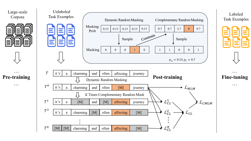
Figure 2: Demonstration of complementary random masking (CRM, in the blue box) and contrastive masked language modeling (CMLM).

3.1 Dynamic Random Masking

Masked language modeling (MLM) is firstly applied in BERT Devlin et al. (2019), where some of the tokens in the input sequence are selected and replaced by a special token “[MASK]”. BERT uniformly selects 15% of the input tokens for replacement, and among the selected tokens, 80% are replaced with “[MASK]”, 10% are left unchanged, and 10% are replaced by a randomly selected vocabulary token. In the original implementation of BERT, random masking and replacement are performed once in the beginning, and the sequences are kept unchanged through pre-training. Liu et al. (2019b) transform this static masking strategy into dynamic random masking (DRM) by generating a masking pattern every time a sequence is fed. That is to say, given an input sequence $T=\{t_{1},t_{2},...,t_{N}\}$, the probability of each token being selected is determined by $p_{m}$, which is fixed to 15% in BERT and RoBERTa.

$$P_{DRM}(t_{n})=p_{m},\ n\in[1,N]$$ (1)

3.2 Complementary Random Masking

It is straightforward to come up with an idea that generates a pair of masked sequences from a single sequence by random masking and applies MLM on each masked sequence to capture token-level similarity, and then perform sequence-level contrastive learning between the two sequences to capture sequence-level similarity. However, it faces a dilemma when applying this idea: setting a small $p_{m}$ would make the pair of masked sequences too similar and make the contrastive learning loss drop to 0 quickly, harming sequence-level contrastive learning. On the other hand, setting a large $p_{m}$ would make each masked sequence collapsed, making it hard for the model to recover the original tokens from “[MASK]” based on the context, which in turn harms token-level contrastive learning.

To address this issue, we decouple the pair of masked sequences, denoted by $T^{0}$ and $T^{1}$, and assign them different masking probabilities $p_{m}$ and $p_{c}$. Specifically, we obtain $T^{0}$ with a small masking probability $p_{m}$ and $T^{1}$ with a larger probability $p_{c}$. Moreover, to avoid a single word being masked by both sequences, which cripples their relevance, we propose complementary random masking (CRM) to generate a pair of complementary masked sequences which maintain a complementary relationship. Concretely, in CRM, we first generate $T^{0}=\{t_{1}^{0},t_{2}^{0},...,t_{N}^{0}\}$ with DRM Liu et al. (2019b) from the original sequence $T$, and generate $T^{1}$ with an extra constraint: the masking probability $P_{CRM}(t_{n})$ will be set to $p_{c}$ if and only if $t_{n}^{0}$ has not been selected in $T^{0}$. Otherwise, it will be set to 0. The process of CRM is described in Figure 2.

$$\mathclap{P_{CRM}(t_{n})=\begin{cases}p_{c},&\text{$t_{n}^{0}$ was not selected in~{}}T^{0}\\ 0,&\text{otherwise}\end{cases}}$$ (2)

CRM is aimed to generate a complementary pair of masked sequences: If $p_{c}=1$, all tokens that are not selected in $T^{0}$ will be selected in $T^{1}$. Reducing $p_{c}$ can soften this complementary relationship and make the two sequences overlap increasingly.

3.3 Contrastive Masked Language Modeling

We propose contrastive masked language modeling, CMLM, based on CRM to realize domain transfer by masked language modeling (MLM) and sequence-level contrastive learning (CL) with pairs of masked sequences. The framework of CMLM is shown in Figure 2, which is described as follows.

Given a batch $\mathcal{T}=\{T_{1},T_{2},...,T_{B}\}$ of input sequences, we firstly apply dynamic random masking (DRM) on each sequence $T_{b}$ to generate a masked sequence $T_{b}^{0}$, and then apply CRM $K$ times to generate $T_{b}^{1},T_{b}^{2},...,T_{b}^{K}$ based on $T_{b}^{0}$ and $T_{b}$:

$$T_{b}^{0}={\rm{DRM}}(T_{b}),\ b\in[1,B]$$ (3)

$$T_{b}^{k}={\rm{CRM}}(T_{b},T_{b}^{0}),\ k\in[1,K]$$ (4)

After obtaining $K+1$ masked sequences from each sequence $T_{b}$ in $\mathcal{T}$, we then compute their representations $H_{b}^{k}\in\mathbb{R}^{N\times d}$ by using an encoder, where $d$ is the hidden size of the encoder:

$$H_{b}^{k}={\rm{Encoder}}(T_{b}^{k}),\ k\in[0,K]$$ (5)

Even though our approach is model-agnostic, in this paper we focus on the Transformer-based pre-trained language model RoBERTa, which is an enhanced version of BERT. Therefore, we employ RoBERTa to implement the $\rm{Encoder}(\cdot)$ function.

To capture token-level similarity, We apply MLM on $H_{b}^{0}$ as Devlin et al. (2019) and Liu et al. (2019b), and compute the loss as follows:

$$\mathcal{L}_{MLM}=\frac{1}{B}\sum^{B}_{b=1}{\rm{MLM}}(H_{b}^{0})$$ (6)

To capture sequence-level similarity, we apply contrastive learning on each $H^{k}_{b}$ and $H^{0}_{b}$, and obtain the loss term $\mathcal{L}_{CL}$. We compare two different implementations of contrastive learning: SimCLR Chen et al. (2020) and SimSiam Chen and He (2020). For SimCLR, $\mathcal{L}_{CL}$ can be calculated as:

$$\mathclap{\mathcal{L}_{CL}=-\frac{1}{K\cdot B}\sum_{k=1}^{K}\sum_{b=1}^{B}{\rm{log}}\frac{e^{{\rm{sim}}(H^{k}_{b},H^{0}_{b})/\tau}}{\sum_{i=1}^{B}e^{{\rm{sim}}(H_{i}^{k},H_{b}^{0})/\tau}}}\quad$$ (7)

where $\tau$ is a temperature parameter.

Following Gunel et al. (2021), we take the first token representation $h_{b}^{k}\in R^{d}$ of $H_{b}^{k}$ to calculate the similarity between $H^{k}_{i}$ and $H^{0}_{j}$ as follows.

$${\rm{sim}}(H^{k}_{i},H^{0}_{j})=\frac{h^{k}_{i}}{||h^{k}_{i}||_{2}}\cdot\frac{h^{0}_{j}}{||h^{0}_{j}||_{2}}$$ (8)

SimSiam is similar to SimCLR except without using negative pairs and has a negative loss value. To be consistent with $\mathcal{L}_{MLM}$ and $\mathcal{L}_{CL}$, we define the loss function of SimSiam as follows:

$$\mathclap{\mathcal{L}_{CL}=\frac{1}{K\cdot B}\sum_{k=1}^{K}\sum_{b=1}^{B}e^{-\frac{1}{2}(D(z_{b}^{k},h_{b}^{0})+D(z_{b}^{0},h_{b}^{k}))}}\quad$$ (9)

where $z^{k}_{b}$ and $D(z,h)$ are defined as:

$$z_{b}^{k}=W_{2}\cdot{\rm{gelu}}(W_{1}\cdot h_{b}^{k})$$ (10)

$$D(z,h)={\rm{sim}}(z,stopgrad(h)).$$ (11)

Here, $W_{1},W_{2}\in R^{d\times d}$ are learnable parameters, ${\rm{sim}}(\cdot)$ is similar to Equation 8, and ${\rm{Stopgrad}}(\cdot)$ is a stop-gradient operation which is crucial for SimSiam Chen and He (2020).

Finally, we combine $\mathcal{L}_{MLM}$ and $\mathcal{L}_{CL}$ for contrastive masking language modeling:

$$\mathcal{L}_{CMLM}=\mathcal{L}_{MLM}+\alpha\cdot\mathcal{L}_{CL}$$ (12)

where $\alpha$ is a tunable hyper-parameter.

3.4 Relationship to Existing Approaches

Among existing approaches, the closest one to ours is CSSL Pre-training Fang and Xie (2020). We can implement CSSL Pre-training by slightly modifying Equation 3 and 12 to following ones:

$$T_{b}^{k}={\rm{back}}(T_{b}),\ k\in[0,1]$$ (13)

$$\mathcal{L}_{CSSL}=\mathcal{L}_{CL}$$ (14)

where ${\rm{back}}(T)$ means back-translation of $T$. And other equations stay the same. By comparing these equations, we note that CMLM can be considered as: (1) replacing back-translation with CRM, which not only reduces the computational cost but also prevents the model from depending on the translation systems; (2) adding $\mathcal{L}_{MLM}$ to implement token-level contrastive learning, which is shown to be crucial in Section 5.2; (3) easily extending one pair of positive samples to $K$ pairs, which can be attributed to the nature of random masking.

As for the loss term, both Giorgi et al. (2020) and Wu et al. (2020) use similar terms to ours for pre-training: $\mathcal{L}_{total}=\mathcal{L}_{MLM}+\mathcal{L}_{CL}$, where $\mathcal{L}_{MLM}$ captures token-level similarity and $\mathcal{L}_{CL}$ captures sequence-level similarity. The main difference between these methods and ours is that we use differently masked sequences from the same sequence as a positive pair, while Giorgi et al. (2020) use position-related segments (overlapping, adjacent or subsumed) and Wu et al. (2020) use sequences by different deformations as the positive pair.

4 Experiment

4.1 Tasks: GLUE

We evaluate our model on the GLUE benchmark Wang et al. (2018), which contains 9 natural language understanding tasks that can be divided into three categories: (1) single sentence tasks: CoLA and SST-2; (2) similarity and paraphrase tasks: MRPC, QQP, and STS-B; (3) inference tasks: MNLI, QNLI, RTE, and WNLI. All of them are classification tasks except STS-B, so we eliminate it to focus on the classification tasks. WNLI has a small development set (70 examples) and is also ignored. MNLI contains two evaluation sets. One, denoted as MNLI, is from the same sources as the training set, and the other, denoted as MNLI-MM, is from different sources than the training set.

To simulate few-shot scenes of different degrees, we randomly select 20, 100, and 1000 examples respectively from these tasks as our training sets following recent work Gunel et al. (2021). For each subset in each task, we sample 5 times with replacement and obtain 15 training sets for each task. As for the development set and test set, we randomly select 500 examples from the original development set as our development set and take the remaining as our test set. Since QQP contains too many examples (40k) in the original development set, we randomly select 2000 from the remaining examples after sampling our development set as our test set. Note that all the 15 training sets in each task share the same development and test sets.

4.2 Model: RoBERTa

As mentioned above, we take RoBERTa to implement our encoder in Equation 5. The base version of RoBERTa, Roberta-base, which contains 12 Transformer blocks with 12 self-attention heads, is employed. All the blocks have the same hidden size 768. The input sequence is either a segment or two segments separated by a special token “[$\backslash$s]”, while “[s]” is always the first token. We take the implementation and pre-trained weights from Huggingface Transformers library Wolf et al. (2020).

	CoLA	SST-2	MNLI	MNLI-MM	QNLI	RTE	MRPC	QQP
Metric	mcc	acc	acc	acc	acc	acc	acc	acc
data size = 20
FT	0.0751$\pm$6.26	0.6604$\pm$6.38	0.3578$\pm$1.70	0.3652$\pm$1.96	0.6163$\pm$3.46	0.5281$\pm$4.07	0.6747$\pm$2.23	0.6777$\pm$3.67
SCL	0.1105$\pm$8.30	0.6964$\pm$6.24	0.3684$\pm$2.85	0.3751$\pm$3.41	0.6191$\pm$3.55	0.5082$\pm$7.75	0.6631$\pm$1.15	0.6947$\pm$2.35
CSSL	0.0795$\pm$4.13	0.6609$\pm$5.98	0.3640$\pm$2.06	0.3686$\pm$2.69	0.6064$\pm$3.26	0.5264$\pm$7.10	0.6638$\pm$1.64	0.6514$\pm$2.99
TAPT	0.0860$\pm$7.64	0.7326$\pm$4.99	0.3616$\pm$2.12	0.3689$\pm$2.40	0.6146$\pm$3.60	0.5437$\pm$5.06	0.6552$\pm$1.64	0.6584$\pm$3.33
CMLM (ours)	0.0902$\pm$8.65	0.7371$\pm$5.64	0.3633$\pm$2.15	0.3701$\pm$2.57	0.6231$\pm$3.60	0.5437$\pm$4.57	0.6586$\pm$1.41	0.6541$\pm$3.89
data size = 100
FT	0.2176$\pm$7.78	0.8405$\pm$2.71	0.4361$\pm$2.50	0.4526$\pm$2.94	0.6820$\pm$2.56	0.5879$\pm$4.82	0.7099$\pm$1.72	0.7511$\pm$1.72
SCL	0.2467$\pm$5.46	0.8455$\pm$1.38	0.4499$\pm$3.30	0.4627$\pm$3.84	0.6765$\pm$2.47	0.5835$\pm$6.41	0.7063$\pm$1.45	0.7461$\pm$1.63
CSSL	0.1719$\pm$7.90	0.8401$\pm$1.71	0.4185$\pm$2.98	0.4298$\pm$3.55	0.6701$\pm$1.89	0.5532$\pm$5.10	0.7038$\pm$1.58	0.7274$\pm$1.85
TAPT	0.2626$\pm$6.03	0.8496$\pm$2.52	0.4508$\pm$2.60	0.4682$\pm$2.80	0.6970$\pm$1.63	0.6095$\pm$6.60	0.6987$\pm$1.77	0.7429$\pm$2.13
CMLM (ours)	0.2663$\pm$6.97	0.8525$\pm$1.95	0.4530$\pm$2.75	0.4683$\pm$3.00	0.6980$\pm$1.67	0.6147$\pm$6.36	0.6933$\pm$1.90	0.7479$\pm$2.16
data size = 1000
FT	0.4216$\pm$3.13	0.8996$\pm$0.97	0.7048$\pm$1.19	0.7168$\pm$1.17	0.7681$\pm$1.07	0.7472$\pm$2.50	0.8223$\pm$1.22	0.7934$\pm$0.90
SCL	0.2758$\pm$11.94	0.8991$\pm$1.04	0.5020$\pm$3.81	0.5089$\pm$4.09	0.7449$\pm$1.22	0.7100$\pm$5.44	0.7157$\pm$6.83	0.7853$\pm$0.77
CSSL	0.4069$\pm$3.53	0.8993$\pm$1.38	0.6900$\pm$1.37	0.7048$\pm$1.39	0.7760$\pm$0.97	0.7082$\pm$5.30	0.8261$\pm$1.70	0.7881$\pm$1.00
TAPT	0.4362$\pm$3.46	0.9016$\pm$0.70	0.7074$\pm$1.79	0.7203$\pm$1.68	0.7689$\pm$0.72	0.7524$\pm$4.06	0.8214$\pm$1.14	0.7890$\pm$0.82
CMLM (ours)	0.4374$\pm$2.06	0.9023$\pm$0.88	0.7110$\pm$2.00	0.7247$\pm$1.84	0.7719$\pm$0.91	0.7610$\pm$3.28	0.8223$\pm$0.82	0.7891$\pm$0.90

Table 1: Results on the GLUE benchmark with 20, 100 and 1000 training examples, respectively, and compared with baseline (FT: Liu et al. (2019b)) and several recent post-training or contrastive learning methods (SCL Gunel et al. (2021), CSSL Fang and Xie (2020), TAPT Gururangan et al. (2020)). Unit of standard deviation is $10^{-2}$.

4.3 Training Details

For the fine-tuning of all approaches to be reported below, unless otherwise specified, we use AdamW Loshchilov and Hutter (2019) with a learning rate of 1e-5 and epochs of 350, 100, 10 for subsets sized 20, 100, 1000, respectively. This setting is based on previous empirical results Zhang et al. (2021); Mosbach et al. (2021), which show that fine-tuning with a small learning rate and more epochs stabilizes the performance of a model in few-shot scenes. We set the batch size to 16 and dropout rate to 0.1, and save model parameters every 100 update steps and pick the best based on validation.

For post-training of CMLM, we apply AdamW with a learning rate of 1e-5 and epochs of 200, 50, 5 for subsets sized 20, 100, 1000, respectively. For a fair comparison with other approaches, we set $K$ in Equation 3 to 1 and the batch size to 8, where the maximum GPU memory usage is approximately equal to that of fine-tuning. For the implementation of $\mathcal{L}_{CL}$, we choose SimSiam for it consumes less computation. For $p_{m}$ in Equation 1, we follow Liu et al. (2019b) and set it to 0.15. We conduct a grid-based search for hyper-parameters with $\alpha\in\{0.01,0.1,0.3,0.5,0.7,1\}$ (Equation 12) and $p_{c}\in\{0.1,0.3,0.5,0.7,0.9\}$ (Equation 2), and find that the combination of $\alpha=0.5$ and $p_{c}=0.7$ performs the best on the development set.

For the baselines to be introduced below, we follow the same fine-tuning and post-training settings as our CMLM, with only several method-specific hyper-parameters unchanged.

4.4 Baseline Approaches

As mentioned in Section 2.2 and 2.3, there have been works trying to add extra loss terms in fine-tuning or to insert a post-training phase in between pre-training and fine-tuning. To make a comprehensive comparison, we employ the following approaches as our baselines: (1) fine-tuning (FT) Liu et al. (2019b), which directly fine-tunes a model with cross-entropy loss; (2) fine-tuning with SCL (SCL) Gunel et al. (2021), which fine-tunes a model with cross-entropy loss and supervised contrastive loss; (3) post-training with CSSL (CSSL) Fang and Xie (2020), which post-trains a model with contrastive self-supervised learning loss; (4) post-training with MLM (TAPT) Gururangan et al. (2020), which post-trains a model with MLM loss and is equal to CMLM when $\alpha=0$. Comparing with recent works Fang and Xie (2020); Gunel et al. (2021) that take only the conventional either BERT or RoBERTa as their baseline, we consider a few more baselines to obtain more conclusive results.

4.5 Evaluation Details

In few-shot scenes, the distribution of the training set may deviate from the test set seriously. Gunel et al. (2021) pick the top-3 results from all combinations of training sets and model seeds for each task. Differently, for each data size of 20, 100, and 1000 described in Section 4.1, we train our model with random seeds {31, 42, 53} for the 5 training subsets, and calculate the mean and standard deviation of the 15 test results. We assume this is a better way to evaluate the overall effect of our model.

4.6 Few-Shot Results

In Table 1, we report our few-shot results on the GLUE tasks with 20, 100, and 1000 training examples, respectively. Five observations can be made from the table. First, CMLM obtains superior performance on the datasets with 100 and 1000 examples, surpassing the baselines in 13 of 16 tasks. Since we use the same hyper-parameters for these approaches and report the average results over 3 random seeds and 5 randomly sampled training sets, these results are convincing. Second, on the dataset with 20 training examples, CMLM only surpasses the other approaches in 3 of 8 tasks. Training a model with only 20 examples is very unstable, and the test results of the baseline approaches indeed show large deviations across different training sets. Third, we find that post-training with only $\mathcal{L}_{MLM}$ Xu et al. (2019); Gururangan et al. (2020) can achieve competitive results with the baselines, showing the effectiveness of this widely-used approach. Fourth, SCL Gunel et al. (2021) has extremely poor performance on CoLA, MNLI, and MRPC when the data size is 1000, which is beyond our expectation. In the original paper, the authors of SCL only report the top-3 results from combinations of model seeds and train sets. So we speculate this under-performance might come from the instability of SCL in few-shot settings. Fifth, CSSL Fang and Xie (2020) performs even worse than FT when the data size is either 20 or 100 but achieves competitive results when the data size is 1000. CSSL is designed for full-size GLUE tasks and might not be suitable for the few-shot scenes.

4.7 Full-Size Results

To verify whether post-training with CMLM can still achieve desirable results when sufficient labeled examples are available, we conduct experiments on the RTE (2.5k), MRPC (3.7k), CoLA (8.5k), SST-2 (67k), and QNLI (106k) tasks with their full-size training sets. We set the learning rate to 3e-5 for both post-training and fine-tuning and set the epoch to 3. Other hyper-parameters remain the same as in Section 4.3. Experiment results are shown in Table 2, from which we can note that CMLM maintains its superiority on RTE and CoLA but fails on MRPC, SST-2, and QNLI. TAPT performs better on tasks with more training examples, which can be explained by the better generalizability of token-level representation, though it demands more training steps to learn well. Note that CMLM is specifically proposed for few-shot settings, so the experiments in the full-size setting are only to evaluate it from different perspectives and make a comprehensive comparison with baselines.

	RTE	MRPC	CoLA	SST-2	QNLI
metric	acc	acc	mcc	acc	acc
data-size	2.5k	3.7k	8.5k	67k	106k
FT	0.7403	0.8623	0.5552	0.9319	0.9043
SCL	0.6753	0.7393	0.5329	0.9373	0.9002
CSSL	0.6623	0.8713	0.5217	0.9310	0.8904
TAPT	0.7403	0.8541	0.5519	0.9355	0.9063
CMLM (ours)	0.7446	0.8574	0.5714	0.9310	0.9039

Table 2: Results on the RTE, MRPC, CoLA, SST-2 and QNLI tasks with full-size training sets, and average results over 3 random seeds are reported.

4.8 Additional Unlabeled Examples

We consider the scene where additional unlabeled task examples are provided. We evaluate CMLM on CoLA, SST-2, QNLI, and MRPC with 100 labeled examples for fine-tuning and increase unlabeled examples from 100 to 2500 for post-training. We depict the results on the development sets in Figure 3, from which two observations can be made. First, the performance generally increases with the number of unlabeled examples grows, showing the helpfulness of unlabeled task examples, which is also confirmed by Gururangan et al. (2020). Second, there are certain fluctuations in the results. We assume they come from the random nature of these additional unlabeled examples, which are sampled from a much larger training set and might severely deviate from the original training set. Moreover, we should acknowledge that adding more unlabeled examples in post-training gains limited improvement compared with adding more labeled examples in fine-tuning. Labeled examples are more treasurable in classification learning.

Figure 3: Results of our model on development sets with increasing numbers of unlabeled examples.

4.9 Hyper-parameter $K$

We evaluate whether increasing $K$ (in Equation 7) can lead to improvement of our model in the few-shot setting. We evaluate CMLM on the CoLA, SST-2, QNLI, and MRPC tasks with 100 training examples by increasing $K$, and the results are depicted in Figure 4. Similar to increasing unlabeled examples, the performance slightly improves on the 5 tasks but has some fluctuations, which is within our expectation. Intuitively, exposing the model to different forms of masked sequences can better reflect the distribution of examples sampled from a large training set, but cannot narrow the deviation between these examples and the original train set.

Figure 4: Results of our model on development sets while the parameter $K$ changes.

5 Ablation Studies

5.1 SimCLR vs SimSiam

As described above, $\mathcal{L}_{CL}$ can be implemented by either Equation 7 or Equation 9, although we implement the latter to conduct the above experiments for its less computational cost. According to Chen and He (2020), SimSiam performs better than SimCLR on ImageNet Deng et al. (2009). It is thus interesting to verify whether the same holds in our situation. We compare SimSiam (CMLM) and SimCLR (w/ SimCLR) on SST-2, CoLA, QNLI and RTE, and the results are reported in Table 3. From the results, we cannot easily conclude which one is better due to their comparable performances, yet further investigation is beyond the scope of this paper. However, we prefer SimSiam due to it consumes less computation and is easier to implement.

5.2 Are MLM & CL Critical for CMLM?

One of the improvements of CMLM over previous works is combining $\mathcal{L}_{MLM}$ and $\mathcal{L}_{CL}$ to implement both token-level and sequence-level contrastive learnings. Here, we verify how the bi-granularity contrastive learnings contribute to the performance differently. We remove $\mathcal{L}_{MLM}$ and $\mathcal{L}_{CL}$ alternatively from $\mathcal{L}_{CMLM}$ and evaluate the resulting model on SST-2, CoLA, QNLI, and RTE with 100 and 1000 training examples, respectively. The results are reported in Table 3. As we can see, the results suffer severe deterioration by up to 7.5% after removing $\mathcal{L}_{MLM}$, while removing $\mathcal{L}_{CL}$ only leads to a drop by up to 1.4%. Although both $\mathcal{L}_{MLM}$ and $\mathcal{L}_{CL}$ contribute to the improvement of CMLM, MLM tends to play a more essential role.

	SST-2	CoLA	QNLI	RTE
Metric	acc	mcc	acc	acc
data size = 100
CMLM	0.8525	0.2663	0.6980	0.6147
w/ SimCLR	0.8586	0.2511	0.6885	0.6355
w/o CL	0.8496	0.2626	0.6980	0.6095
w/o MLM	0.8280	0.2492	0.6873	0.5913
w/o CRM	0.8511	0.2621	0.6920	0.6242
data size = 1000
CMLM	0.9023	0.4374	0.7719	0.7610
w/ SimCLR	0.9041	0.4446	0.7696	0.7732
w/o CL	0.9016	0.4362	0.7689	0.7524
w/o MLM	0.8927	0.3983	0.7623	0.7039
w/o CRM	0.9013	0.4434	0.7698	0.7654

Table 3: Results of ablation study for CMLM. w/ SimCLR means replacing SimSiam with SimCLR, w/o CL and w/o MLM mean removing $\mathcal{L}_{CL}$ and $\mathcal{L}_{MLM}$ terms from $\mathcal{L}_{CMLM}$, respectively, and w/o CRM means replacing CRM with dynamic random masking (DRM).

5.3 Complementary Random Masking vs Dynamic Random Masking

We propose a complementary random masking (CRM) strategy to generate complementary masked sequences $T^{k},\ k\in[1,K]$, based on $T^{0}$, which is generated by dynamic random masking (DRM). Here, we verify whether this complementary nature of $T^{k}$ benefits contrastive learning. We replace CRM in Equation 3 by DRM, and conduct experiments on SST-2, CoLA, QNLI and RTE with 100 and 1000 training examples, respectively. As shown in Table 3, CRM still surpasses DRM on all 8 tasks, with improvement by up to 1.6%. The superiority of CRM mainly comes from fact that it avoids tokens to be masked in both $T^{0}$ and $T^{k}$.

6 Conclusion

In this paper, we proposed a novel post-training objective, CMLM, for pre-trained language models in downstream few-shot scenes. CMLM attempts to combine both token-level and sequence-level contrastive learnings for more efficient domain transfer during post-training. For sentence-level contrastive learning, we developed a random masking strategy, CRM, to generate a pair of complementary masked sequences for an input sequence. Empirical results show that post-training with our CMLM outperforms other recent approaches on the GLUE tasks with 100 and 1000 labeled training examples, respectively. We also conducted extensive ablation studies and showed that both token-level and sequence-level contrastive learnings contribute to the results of CMLM, and that CRM achieves favorable sequence-level contrastive learning over the previous masking strategy. In future work, we will further investigate how token-level and sequence-level contrastive learnings affect domain transfer in post-training and explore more effective methods for sequence-level contrastive learning.

References

- Chen et al. (2020) Ting Chen, Simon Kornblith, Mohammad Norouzi, and Geoffrey Hinton. 2020. A simple framework for contrastive learning of visual representations. In Proceedings of the 37th International Conference on Machine Learning, volume 119 of Proceedings of Machine Learning Research, pages 1597–1607, Virtual. PMLR.
- Chen and He (2020) Xinlei Chen and Kaiming He. 2020. Exploring simple siamese representation learning. arXiv preprint arXiv:2011.10566.
- Deng et al. (2009) J. Deng, W. Dong, R. Socher, L. Li, Kai Li, and Li Fei-Fei. 2009. Imagenet: A large-scale hierarchical image database. In 2009 IEEE Conference on Computer Vision and Pattern Recognition, pages 248–255.
- Devlin et al. (2019) Jacob Devlin, Ming-Wei Chang, Kenton Lee, and Kristina Toutanova. 2019. BERT: Pre-training of deep bidirectional transformers for language understanding. In Proceedings of the 2019 Conference of the North American Chapter of the Association for Computational Linguistics: Human Language Technologies, Volume 1 (Long and Short Papers), pages 4171–4186, Minneapolis, Minnesota. Association for Computational Linguistics.
- Dodge et al. (2020) Jesse Dodge, Gabriel Ilharco, Roy Schwartz, Ali Farhadi, Hannaneh Hajishirzi, and Noah Smith. 2020. Fine-tuning pretrained language models: Weight initializations, data orders, and early stopping. arXiv preprint arXiv:2002.06305.
- Edunov et al. (2018) Sergey Edunov, Myle Ott, Michael Auli, and David Grangier. 2018. Understanding back-translation at scale. In Proceedings of the 2018 Conference on Empirical Methods in Natural Language Processing, pages 489–500, Brussels, Belgium. Association for Computational Linguistics.
- Fang and Xie (2020) Hongchao Fang and Pengtao Xie. 2020. CERT: Contrastive self-supervised learning for language understanding. arXiv preprint arXiv:2005.12766.
- Giorgi et al. (2020) John M Giorgi, Osvald Nitski, Gary D Bader, and Bo Wang. 2020. DeCLUTR: Deep contrastive learning for unsupervised textual representations. arXiv preprint arXiv:2006.03659.
- Gunel et al. (2021) Beliz Gunel, Jingfei Du, Alexis Conneau, and Veselin Stoyanov. 2021. Supervised contrastive learning for pre-trained language model fine-tuning. In International Conference on Learning Representations.
- Gururangan et al. (2020) Suchin Gururangan, Ana Marasović, Swabha Swayamdipta, Kyle Lo, Iz Beltagy, Doug Downey, and Noah A. Smith. 2020. Don’t stop pretraining: Adapt language models to domains and tasks. In Proceedings of the 58th Annual Meeting of the Association for Computational Linguistics, pages 8342–8360, Online. Association for Computational Linguistics.
- Hadsell et al. (2006) R. Hadsell, S. Chopra, and Y. LeCun. 2006. Dimensionality reduction by learning an invariant mapping. In 2006 IEEE Computer Society Conference on Computer Vision and Pattern Recognition (CVPR’06), volume 2, pages 1735–1742.
- Iter et al. (2020) Dan Iter, Kelvin Guu, Larry Lansing, and Dan Jurafsky. 2020. Pretraining with contrastive sentence objectives improves discourse performance of language models. In Proceedings of the 58th Annual Meeting of the Association for Computational Linguistics, pages 4859–4870, Online. Association for Computational Linguistics.
- Jiang et al. (2020) Haoming Jiang, Pengcheng He, Weizhu Chen, Xiaodong Liu, Jianfeng Gao, and Tuo Zhao. 2020. SMART: Robust and efficient fine-tuning for pre-trained natural language models through principled regularized optimization. In Proceedings of the 58th Annual Meeting of the Association for Computational Linguistics, pages 2177–2190, Online. Association for Computational Linguistics.
- Khosla et al. (2020) Prannay Khosla, Piotr Teterwak, Chen Wang, Aaron Sarna, Yonglong Tian, Phillip Isola, Aaron Maschinot, Ce Liu, and Dilip Krishnan. 2020. Supervised contrastive learning. In Advances in Neural Information Processing Systems, volume 33, pages 18661–18673. Curran Associates, Inc.
- Lee et al. (2020) Cheolhyoung Lee, Kyunghyun Cho, and Wanmo Kang. 2020. Mixout: Effective regularization to finetune large-scale pretrained language models. In International Conference on Learning Representations.
- Li et al. (2021) Tian Li, Xiang Chen, Shanghang Zhang, Zhen Dong, and Kurt Keutzer. 2021. Cross-domain sentiment classification with contrastive learning and mutual information maximization. In ICASSP 2021 - 2021 IEEE International Conference on Acoustics, Speech and Signal Processing (ICASSP), pages 8203–8207.
- Liu et al. (2019a) Xiaodong Liu, Pengcheng He, Weizhu Chen, and Jianfeng Gao. 2019a. Multi-task deep neural networks for natural language understanding. In Proceedings of the 57th Annual Meeting of the Association for Computational Linguistics, pages 4487–4496, Florence, Italy. Association for Computational Linguistics.
- Liu et al. (2019b) Yinhan Liu, Myle Ott, Naman Goyal, Jingfei Du, Mandar Joshi, Danqi Chen, Omer Levy, Mike Lewis, Luke Zettlemoyer, and Veselin Stoyanov. 2019b. RoBERTa: A robustly optimized BERT pretraining approach. arXiv preprint arXiv:1907.11692.
- Loshchilov and Hutter (2019) Ilya Loshchilov and Frank Hutter. 2019. Decoupled weight decay regularization. In International Conference on Learning Representations.
- Mosbach et al. (2021) Marius Mosbach, Maksym Andriushchenko, and Dietrich Klakow. 2021. On the stability of fine-tuning BERT: Misconceptions, explanations, and strong baselines. In International Conference on Learning Representations.
- Phang et al. (2018) Jason Phang, Thibault Févry, and Samuel R Bowman. 2018. Sentence encoders on STILTs: Supplementary training on intermediate labeled-data tasks. arXiv preprint arXiv:1811.01088.
- Radford et al. (2018) Alec Radford, Karthik Narasimhan, Tim Salimans, and Ilya Sutskever. 2018. Improving language understanding by generative pre-training (2018).
- Vaswani et al. (2017) Ashish Vaswani, Noam Shazeer, Niki Parmar, Jakob Uszkoreit, Llion Jones, Aidan N Gomez, Ł ukasz Kaiser, and Illia Polosukhin. 2017. Attention is all you need. In Advances in Neural Information Processing Systems, volume 30. Curran Associates, Inc.
- Wang et al. (2018) Alex Wang, Amanpreet Singh, Julian Michael, Felix Hill, Omer Levy, and Samuel Bowman. 2018. GLUE: A multi-task benchmark and analysis platform for natural language understanding. In Proceedings of the 2018 EMNLP Workshop BlackboxNLP: Analyzing and Interpreting Neural Networks for NLP, pages 353–355, Brussels, Belgium. Association for Computational Linguistics.
- Wolf et al. (2020) Thomas Wolf, Lysandre Debut, Victor Sanh, Julien Chaumond, Clement Delangue, Anthony Moi, Pierric Cistac, Tim Rault, Remi Louf, Morgan Funtowicz, Joe Davison, Sam Shleifer, Patrick von Platen, Clara Ma, Yacine Jernite, Julien Plu, Canwen Xu, Teven Le Scao, Sylvain Gugger, Mariama Drame, Quentin Lhoest, and Alexander Rush. 2020. Transformers: State-of-the-art natural language processing. In Proceedings of the 2020 Conference on Empirical Methods in Natural Language Processing: System Demonstrations, pages 38–45, Online. Association for Computational Linguistics.
- Wu et al. (2020) Zhuofeng Wu, Sinong Wang, Jiatao Gu, Madian Khabsa, Fei Sun, and Hao Ma. 2020. CLEAR: Contrastive learning for sentence representation. arXiv preprint arXiv:2012.15466.
- Xu et al. (2019) Hu Xu, Bing Liu, Lei Shu, and Philip Yu. 2019. BERT post-training for review reading comprehension and aspect-based sentiment analysis. In Proceedings of the 2019 Conference of the North American Chapter of the Association for Computational Linguistics: Human Language Technologies, Volume 1 (Long and Short Papers), pages 2324–2335, Minneapolis, Minnesota. Association for Computational Linguistics.
- Zhang et al. (2021) Tianyi Zhang, Felix Wu, Arzoo Katiyar, Kilian Q Weinberger, and Yoav Artzi. 2021. Revisiting few-sample BERT fine-tuning. In International Conference on Learning Representations.