Test of a small prototype of the COMET cylindrical drift chamber

Abstract

The performance of a small prototype of a cylindrical drift chamber (CDC) used in the COMET Phase-I experiment was studied by using an electron beam. The prototype chamber was constructed with alternating all-stereo wire configuration and operated with the He$-$iC₄H₁₀(90/10) gas mixture without a magnetic field. The drift space-time relation, drift velocity, d$E$/d$x$ resolution, hit efficiency, and spatial resolution as a function of distance from the wire were investigated. The average spatial resolution of $150\,\mu$m with the hit efficiency of $99\,\%$ was obtained at applied voltages higher than 1800 V. We have demonstrated that the design and gas mixture of the prototype match the operation of the COMET CDC.

1 Introduction

The COherent Muon to Electron Transition (COMET) experiment at the Japan Proton Accelerator Research Complex (J-PARC) in Tokai, Japan, is to search for the neutrinoless coherent transition of a muon to an electron ($\mu$$-$$e$ conversion) in the field of a nucleus, with its single event sensitivity of $2\times 10^{-17}$, which is more than four orders of magnitude improvement over the current upper limit of $7\times 10^{-13}$ at 90 % C.L. from the SINDRUM II experiment [1]. The COMET experiment is organized as a two-stage project. The first stage, COMET Phase-I, is seeking a sensitivity of $3\times 10^{-15}$ with 3.2-kW proton beam power [2, 3]. It will be carried out at the Hadron Experimental Facility of J-PARC using a bunched 8-GeV proton beam that is slowly extracted from the J-PARC Main Ring.

The main detector system for the $\mu$$-$$e$ conversion search in COMET Phase-I is the Cylindrical Detector (CyDet). It consists of a cylindrical drift chamber (CDC) and a cylindrical trigger hodoscope. The primary function of the CDC is to measure the momentum of $\mu$$-$$e$ conversion electrons. Figure 1 shows a schematic layout of the CyDet. It is located downstream of the muon transport section, and installed within the warm bore of a large 1-T superconducting detector solenoid. The CyDet must accurately and efficiently identify and measure signal electrons of 105 MeV from aluminum target disks whilst suppressing backgrounds. It is designed to avoid high hit rates from the beam particles, background electrons from muon decay-in-orbit (DIO), and low energy protons emitted after the nuclear capture process of negative muons.

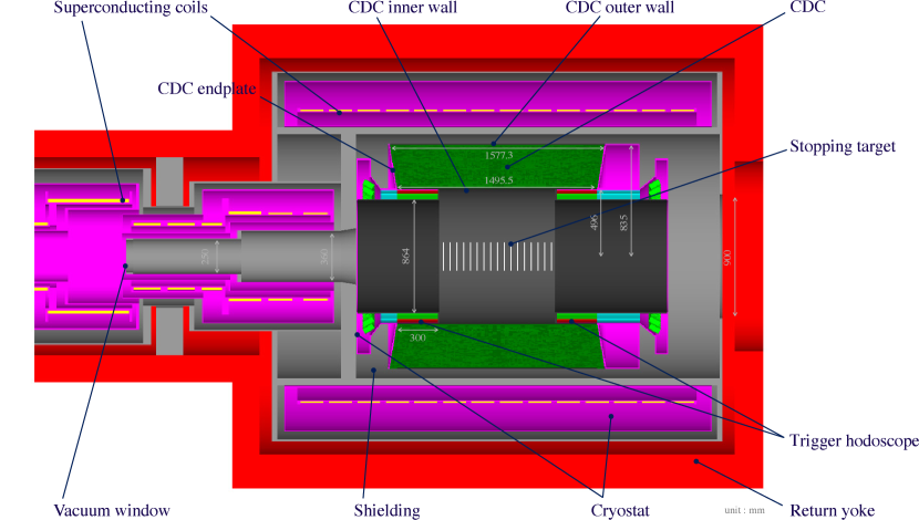
Figure 1: Schematic layout of the cylindrical detector system. A muon beam comes from left and stops in the target disks located in the center of the detector solenoid.

The momentum resolution of CDC should be less than 200 keV/$c$ for the 105-MeV/$c$ electrons in order to distinguish the signal electrons from the DIO electrons. Note that the momentum resolution for the electrons at this momentum is dominated by the multiple scattering effect. In order to suppress this effect, He$-$iC₄H₁₀(90/10) is selected as a gas mixture for its long radiation length of 1313 m [4]. He$-$iC₄H₁₀ was so far used to achieve high-momentum resolution in a low-momentum region in only a few experiments, e.g. KLOE [5] and MEG-II [6] with a ratio of 90/10, and BaBar [7] with 80/20.

A major motivation of this work is to demonstrate that the current design of the cell and wire structure of the CDC with the He$-$iC₄H₁₀(90/10) gas mixture can work in the COMET Phase-I experiment. We constructed a prototype chamber of the CDC and performed a beam test. In this paper, an experimental setup and an analysis method for the CDC prototype test are introduced. Then the drift space-time relation, drift velocity, spatial resolution, hit efficiency, gas gain and d$E$/d$x$ resolution are discussed.

2 Experiment

2.1 A prototype chamber

A detailed specification of CDC can be found in [3]. The outer diameter, inner diameter and length of the CDC are 1.7 m, 1.0 m and 1.6 m, respectively, with a volume of 2 m³. An alternating stereo wire configuration creates a total of 4986 drift cells with 20 concentric layers.

The prototype chamber was manufactured as a small partial copy of the CDC structure. It consists of 79 drift cells with 8 sensitive layers and 1 dummy layer. The purpose of sensitive layers is to detect the ionization electrons, whereas the dummy layer is used to study the effect of crosstalk from the electronics, which is not described in this paper. All the wires are strung with an alternating stereo angle of approximately $\pm 4$ degrees layer by layer. The cell shape is almost square with dimensions of (16.8$\times$16.0) mm². The layout of the cell structure at the center of the longitudinal direction is shown in Figure 2, and pictures of the chamber are shown in Figure 3. The size of the chamber is 600 mm in length, 170 mm in height, 280 mm in width. There are 79 gold-plated tungsten wires with a diameter of 25 $\mu$m as anode wires, and 265 aluminum wires with a diameter of 126 $\mu$m as cathode wires.

The endplates and walls of the chamber are made of aluminum. An engineering tolerance for the position of the wire ends with feedthroughs is less than 50 $\mu$m. There are four aluminized Mylar windows with thickness of 200 $\mu$m in all walls so that the effects of electromagnetic showers by the electron beam to the chamber can be minimized. A positive high voltage (HV) is supplied to the anode wires from one side of the endplates. From the other side, two front-end electronics boards are connected to the anode wires through decoupling capacitors. The electronics boards are covered with an aluminum box to suppress electromagnetic noise.

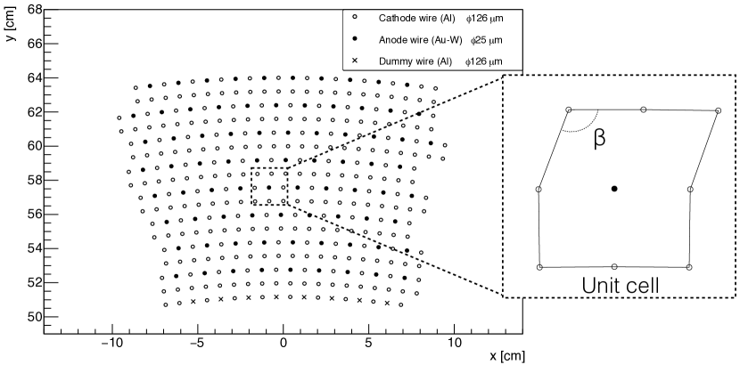
Figure 2: Layout of wire configuration at the center of the chamber together with an expanded view of a unit cell. The cell deformation angle, $\beta$, ranges approximately 60 to 120 degrees depending on the $z$ position of the chamber.

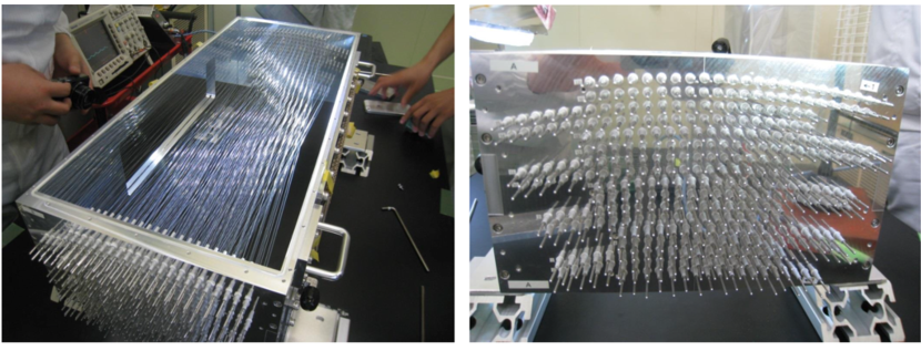
Figure 3: Pictures of the prototype chamber with dimensions of $(600\times 170\times 280)$ mm³.

The front-end readout electronics were fabricated based on the Readout Electronics for the Central Drift Chamber of Belle-II Experiment (RECBE) [8, 9] with some modifications. There are two outputs from the frontend amplifier–shaper–discriminator ASIC of RECBE [10]: one is discriminated inside the ASIC and converted to timing information with 960-MHz TDC in an FPGA; therefore the time was digitized in a unit of 1.04 ns. The other is used to measure the charge with 10-bit, 30-MHz sampling rate ADC. Since the typical signal width is several tens of nanoseconds, the whole signal is sufficiently covered with the ADC time range of 1 $\mu$s. The SiTCP protocol [11] is used to transmit the event data to a data-acquisition computer via Gigabit Ethernet fiber link.

2.2 Experimental setup

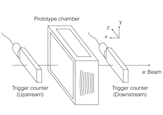
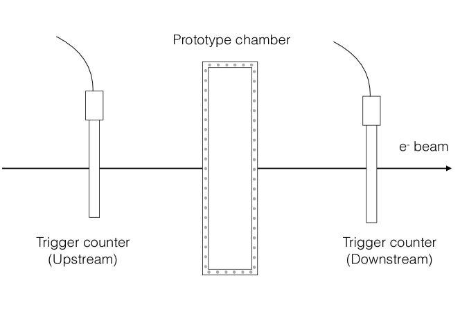
Figure 4: Schematic layouts of the experimental setup. The upper figure is a side view and the lower figure is a top view.

The test experiment with an electron beam was performed in the Laser Electron Photon facility at SPring-8 (LEPS) [12, 13], Japan. A photon beam of backward Compton scattering from UV laser, of 1.5 to 2.4 GeV was used to generate a 1-GeV electron beam by colliding with a lead converter. The momentum selection of the electron beam was made with a dipole magnet located downstream of the lead converter. Two plastic scintillating counters of ($300\times 90\times 10$) mm³ size were installed at both upstream and downstream of the prototype chamber. Schematic layouts of the experimental setup is shown in Figure 4. There was no significant magnetic field around the prototype chamber in this setup. The beam spreads over the whole chamber in the horizontal direction, whereas the vertical spread of the beam is around 5 to 6 cm.

The timing and charge of wire hits were measured by RECBE and recorded by a data-acquisition computer using DAQ Middleware [14]. The event trigger was issued by a coincidence of signals from the two trigger counters. The average trigger rate was around 4–5 kHz. The high voltage and discrimination threshold were scanned at every 500 thousands events. A detailed list of the experimental conditions is shown in Table 1.

The gas flow rate is controlled at 20 cc/min. As the gas gain of the chamber is sensitive to the environmental condition, the temperature of $26.0\pm 0.5$ ^∘C, the atmospheric pressure of $979\pm 3$ hPa, and the humidity of $53\pm 5$ % were maintained during the tests. This level of variation in temperature and pressure affects the gas density at most by 0.5%; and according to [15], its effect on gas gain variation is estimated to be less than 4%.

Table 1: List of the experimental conditions. Here the discrimination threshold is defined as the analog output of the ASIC after amplification.

Gas mixture	High voltage [V]	Threshold [mV]
He$-$iC4H10(90/10)	1650–1830	10–30

3 Data Analysis

3.1 Track reconstruction

The signal waveforms were recorded in 32 sampling points of ADC with a 33-ns interval. The ADC values of each channel were numerically summed up separately after subtracting a pedestal level to obtain charge information; we call this as ADC sum hereafter. In the beginning of the data analysis, the wire hits were classified by their ADC sum. A typical ADC sum distribution of a cell is shown in Figure 5. Since signals and noises were clearly separated, a cut for signal hit identification was applied based on the ADC sum for each drift cell. We used a calibration function obtained in an earlier electronics test for converting the ADC sum to charge.

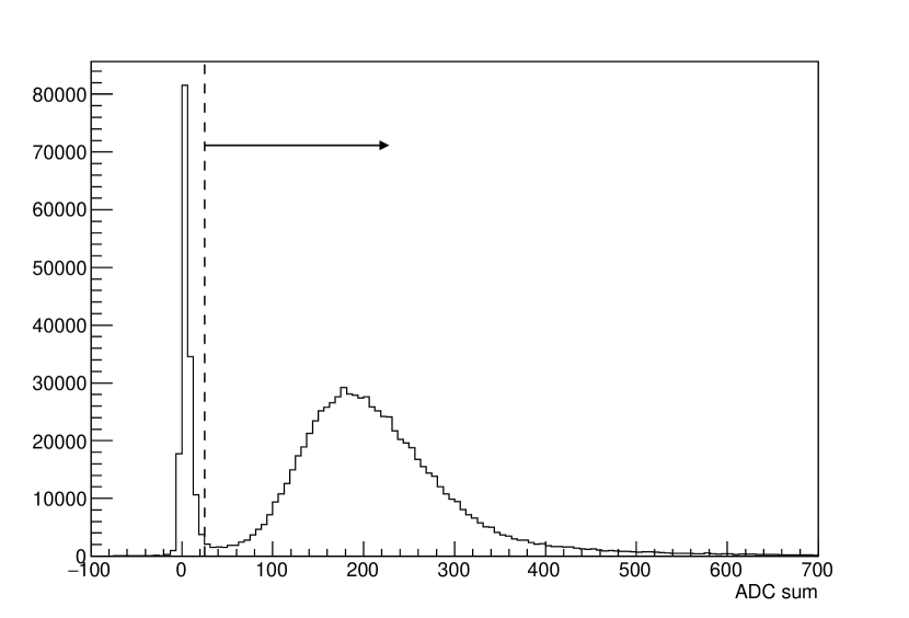
Figure 5: ADC sum distribution measured at a drift cell for He$-$iC₄H₁₀(90/10) at 1800 V with 10-mV threshold. In this case the ADC sum larger than 25 was selected, as indicated by the dashed line.

In order to test the performance of a specific cell and layer, the hits in the dummy layer and a layer to be tested were excluded from the track reconstruction to avoid bias. Events with the total number of signal hits larger than 6 were used for track reconstruction. Using a drift space-time relation, which will be discussed in the following subsection, drift time was converted into the drift distance, $d$. The residual of a signal hit was defined as $r=d-d^{\textrm{fit}}$, where $d^{\textrm{fit}}$ is the distance of the closest approach from the reconstructed track to the anode wire in the hit cell. Excluding the layer to be tested, the sum of normalized residuals of signal hits was defined as the $\chi^{2}$ of the reconstructed track:

$$\chi^{2}=\sum_{i}\Bigg{(}\frac{d_{i}-d_{i}^{\textrm{fit}}}{\sigma(d_{i})}\Bigg{)}^{2},$$ (1)

where $i$ is a hit index, and $\sigma(d)$ denotes spatial resolution as a function of the distance $d$, the details of which will be discussed in Section 4.2. A $\chi^{2}$–minimization algorithm was applied to obtain a realistic reconstructed track. In the following study, the central forth layer was chosen as the layer to be tested, so as to minimize a tracking error, unless otherwise noted.

3.2 Drift space-time relation

A drift space-time (hereafter $s$-$t$ ) relation was studied by an iterative procedure starting from an initial value obtained from Garfield++ [16]. A typical $s$-$t$ distribution is shown in Figure 6. The $s$-$t$ relation was calibrated layer by layer. The distribution was averaged over 200-$\mu$m intervals near the anode wire and over 3-ns intervals near the cell boundary. To get a parameterized $s$-$t$ relation, the averaged distribution was then fitted by piecewise continuous third-order polynomial functions connecting four different drift time regions. An example of the $s$-$t$ relation fitting is shown in Figure 7. The $s$-$t$ relations for data sets with different high voltages or thresholds were calibrated separately, and applied for the following analysis procedures accordingly.

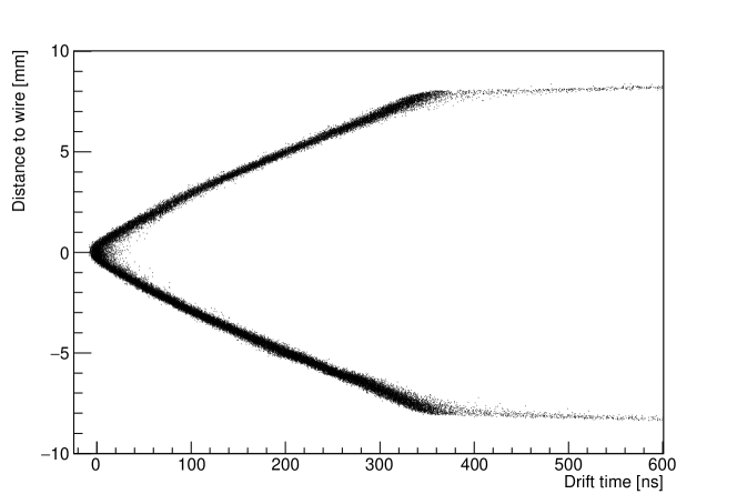
Figure 6: Space-time distribution of the central layer obtained for He$-$iC₄H₁₀(90/10) at 1800 V with 10 mV threshold.

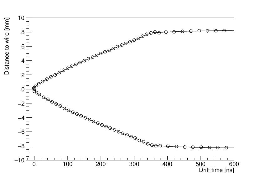
Figure 7: Fitted space-time relation for He$-$iC₄H₁₀(90/10) at 1800 V with 10-mV threshold. The open circles represent the averaged space-time distribution, and the solid line is the fitted function. Notice that the number of circles shown here is less than the used intervals for a better visualization.

3.3 Drift velocity

The drift velocity was calculated by taking derivatives of the $s$-$t$ relation as a function of the distance from the wire. The local electric field in a drift cell was calculated by using the Garfield++ simulation. Then we obtained the drift velocity as a function of the local electric field as shown in Figure 8. The drift velocity in He$-$iC₄H₁₀(90/10) gas mixture is unsaturated near 1000 V/cm/atm. Figure 8 also shows other results of calculations [17] and experimental measurements [18, 19, 20] together with Garfield++ simulation. In the Garfield++ simulation, we considered an experimental uncertainty of gas mixture ratio as ranging from $89.6:10.4$ to $90.4:9.6$, and an uncertainty of water vapor contamination as ranging from 0 to 0.12%  . All data show good agreement; the minimal deviations could be justified within small differences in operating conditions, such as pressure, temperature, gas mixture ratio, and water vapor contamination.

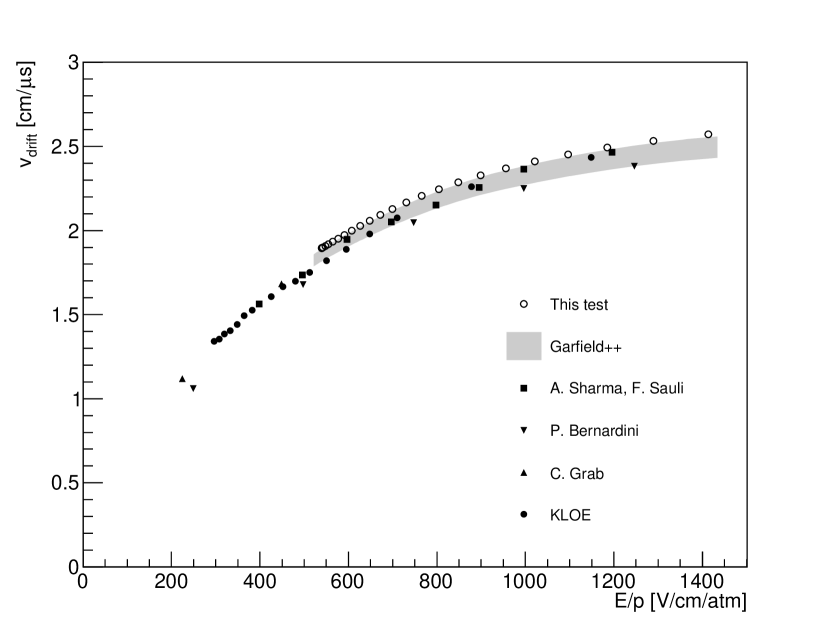
Figure 8: Drift velocity versus the electric field for He$-$iC₄H₁₀(90/10) at 1 atm by comparing with Garfield++ simulation, calculations of Sharma–Sauli [17], and experiments of P. Bernardini [18], C. Grab [19], and a KLOE-CDC prototype [20]. For the band of Garfield++ simulation, the lower boundary corresponds to the gas mixture ratio between He and iC₄H₁₀ at $90.4:9.6$, and the upper boundary corresponds to the gas mixture ratio at $89.6:10.4$ with 0.12% water vapor.

4 Results and Discussion

4.1 Scan of applied high voltage

In order to determine an optimal operation high voltage, the spatial resolution and cell hit efficiency were studied as a function of applied high voltage. The intrinsic spatial resolution was extracted from the standard deviation of residual distributions, $\sigma_{\textrm{total}}$, by subtracting a tracking error in quadrature. Since the tracking error is caused by extrapolating or interpolating the reconstructed track, it was estimated from a simulation with assumed intrinsic spatial resolution. Comparing the simulation with the experimental data, the tracking error was derived to be 94 $\mu$m for the central layer. The cell hit efficiency was defined as the ratio of the number of hits with the residual within $\pm 5\,\sigma_{\textrm{total}}$ to the number of tracks passing through the cell.

The results are shown in Figure 9 for high voltages from 1650 to 1830 V. Note that an optimal threshold value which gave the best spatial resolution was selected for each high-voltage data set. The plateau-like behavior of efficiency and spatial resolution are consistent with other literatures [5, 21]. We obtained the best spatial resolution of 150 $\mu$m with 99% hit efficiency at the voltages higher than 1800 V.

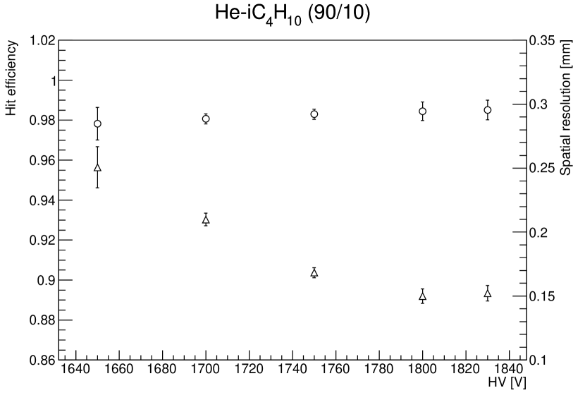
Figure 9: Cell hit efficiency (circles) and intrinsic spatial resolution (triangles) as a function of the applied voltage for He$-$iC₄H₁₀(90/10).

4.2 Spatial resolution

The spatial resolution varies depending on the distance from the anode wire. Detailed contributions to spatial resolution were studied using a similar method of [20]. The components of spatial resolution can be grouped into primary ionization statistics ($\sigma_{\textrm{ion}}$), electron longitudinal diffusion ($\sigma_{\textrm{diff}}$), and electronics time resolution ($\sigma_{\textrm{ele}}$):

$$\sigma=\sqrt{\sigma_{\textrm{ion}}^{2}+\sigma_{\textrm{diff}}^{2}+\sigma_{\textrm{ele}}^{2}}.$$ (2)

The contribution of primary ionization statistics was estimated from a Monte Carlo simulation. Primary ions were generated according to $\exp(-n_{\textrm{p}}y)$, where $n_{\textrm{p}}$ is the number of primary ions per unit length, and $y$ is the track path length in a drift cell. $\sigma_{\textrm{ion}}$ was estimated from the standard deviation of the difference between the distance from anode wire to the track and to the closest ionization point. Therefore, $\sigma_{\textrm{ion}}$ was obtained as a function of the distance to wire and $n_{\textrm{p}}$.

The function of $\sigma_{\textrm{diff}}$ follows an approximation of a classical diffusion theory based on the Boltzmann statistics: $\sigma_{\textrm{diff}}(x)=\sqrt{(2Dx/v)}$, where $D$, $x$, and $v$ are the diffusion coefficient, drift distance, and average drift velocity, respectively. For $\sigma_{\textrm{ele}}$, the main contributions come from the time resolution of the readout electronics and time walk effect of signals. The time resolution was determined from specification of the electronics to be $1.04/\sqrt{12}$ ns, which corresponds to 10 $\mu$m, whereas the time walk effect was found to be negligible by choosing a low threshold level of electronics.

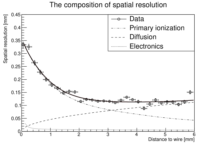
Figure 10: Spatial resolution as a function of distance to the anode wire for He$-$iC₄H₁₀(90/10) at 1800 V with 10-mV threshold. The open circles represent the experimental data. The solid line indicates the fitting results. The dot–dashed line, dashed line and dotted line show the contribution of the primary ionization, longitudinal diffusion, and electronics time resolution, respectively.

Figure 10 shows the spatial resolution as a function of distance to the anode wire together with the fitting result by Eq.2. The fitting result shows that the number of primary ionization $n_{\textrm{p}}=14.2\pm 0.2$ cm^-1. For comparison with other results, the $n_{\textrm{p}}$ value was scaled from the 1-GeV electron in our experiment to minimum ionizing particles taking the energy loss difference into account. Using the photo-absorption ionization model [22], we obtained $n_{\textrm{p}}=9.9\pm 0.1$ cm^-1 for minimum ionizing particles. Note that the uncertainty is only statistical, and systematic uncertainties are not taken into account. The result is slightly smaller but in a decent agreement with 12.7 cm^-1 computed by Sharma and Sauli [17] and $12.3\pm 0.2$ cm^-1 reported in  [20].

The fitting result also gives $D/v=(1.05\pm 0.04)\times 10^{-4}$ cm for the ratio of the diffusion coefficient to the drift velocity. The value corresponds to 112 $\mu$m for 0.6 cm of drift. It was found that the deterioration of the spatial resolution near the anode wire is due to the statistical fluctuation of primary ionization, whereas the longitudinal diffusion dominates in the long drift distance.

4.3 Gas gain

Once the track was reconstructed, the measured charge at each drift cell was then divided by the path length of the track in the drift cell (hereafter $Q$). The gas gain $G$ is computed as $Q/(n_{\textrm{t}}e)$, where $n_{\textrm{t}}$ is the total number of electron–ion pairs per unit length, and $e$ denotes the elementary charge. To avoid the non-linear effect in the Landau tail of the distribution of $Q$ and $n_{\textrm{t}}$ contributed by the electronics and the space charge effect, we took the most probable values (MPV) for each distribution in one drift cell. The $n_{\textrm{t}}^{\textrm{MPV}}$ was computed as $(dE/dx)^{\textrm{MPV}}/W_{\textrm{I}}$, where $(dE/dx)^{\textrm{MPV}}$ is the most probable energy deposition per unit length in one drift cell, and $W_{\textrm{I}}$ is the average ionization energy per ion pair. Ignoring the Penning effect, $W_{\textrm{I}}$ in He$-$iC₄H₁₀(90/10) was computed as 29.3 eV based on the He and iC₄H₁₀ properties given in [23]. According to the photon absorption ionization model [22], $(dE/dx)^{\textrm{MPV}}$ for an 1-GeV electron in this gas mixture is computed to be 0.70 keV/cm, therefore $n_{\textrm{t}}^{\textrm{MPV}}$ = 23.9 cm^-1. The gas gain was then calculated for data sets at different high voltages using the measured $Q^{\textrm{MPV}}$. Figure 11 shows the relationship between the gas gain and the applied high voltage. A linear relation in a logarithmic scale can be observed as expected.

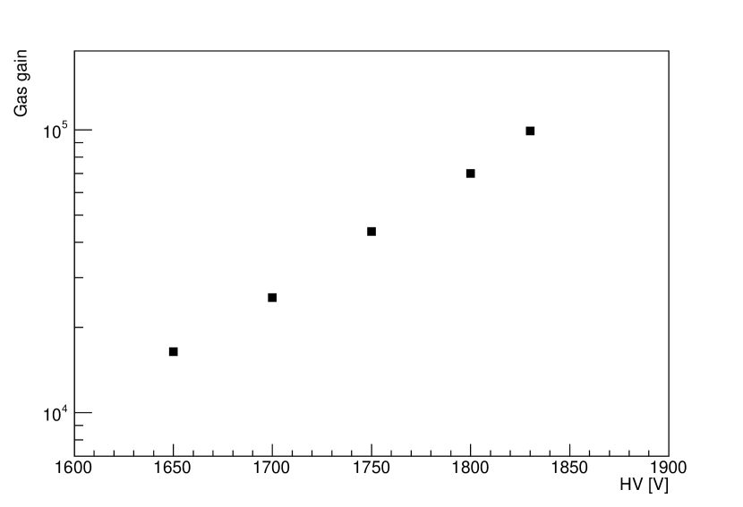
Figure 11: Relation between gas gain and high voltage for He$-$iC₄H₁₀(90/10) with 10-mV threshold.

4.4 d$E$/d$x$ resolution

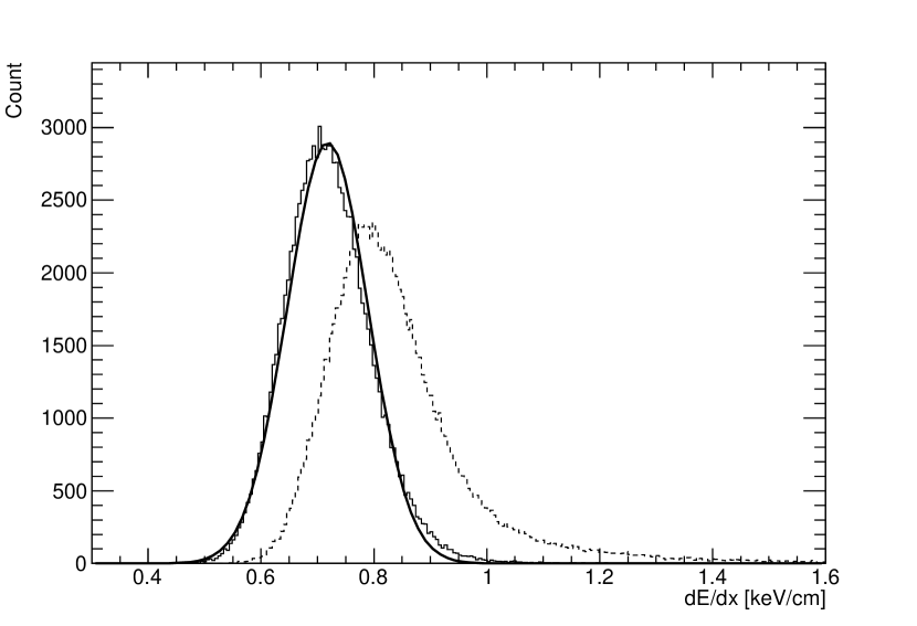
Figure 12: d$E$/d$x$ distribution measured for tracks with 10 samples using data taken from He$-$iC₄H₁₀(90/10) at 1800 V with 10-mV threshold. The solid and dashed lines denote histograms with 80$\,\%$ truncated mean and without truncation, respectively.

For the measurement of the d$E$/d$x$ resolution, tracks with arbitrary lengths by combining hits in reconstructed events were simulated. To avoid Landau tail of collected charge distribution worsening the d$E$/d$x$ resolution, the truncated mean technique was applied [24]. A comparison of the d$E$/d$x$ distribution with and without truncation is shown in Figure 12. We found that the best d$E$/d$x$ resolution can be achieved by accepting 80$\,\%$ of hits in a track, as shown in Figure 13.

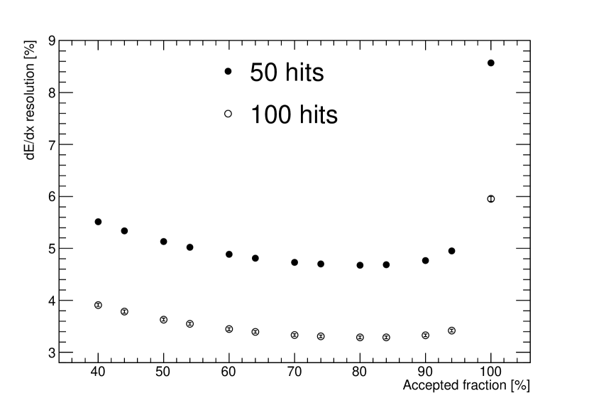
Figure 13: d$E$/d$x$ resolution for tracks with 50 and 100 samples using data taken from He$-$iC₄H₁₀(90/10) at 1800 V with 10-mV threshold as a function of the truncation ratio.

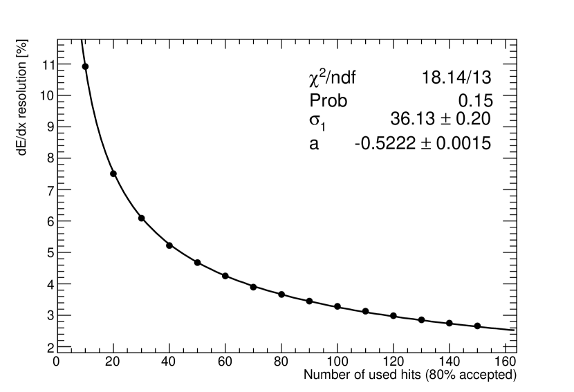
Figure 14: d$E$/d$x$ resolution of tracks with different number of samples taken from He$-$iC₄H₁₀(90/10) at 1800 V with 10 mV threshold. The solid line denotes the fitting result with Eq. 3; here $\sigma_{0}x^{b}$ is absorbed into $\sigma_{1}$ with $x=1.6$ cm.

The d$E$/d$x$ resolution can be parameterized as [25]

$$\sigma_{\textrm{d}E/\textrm{d}x}=\sigma_{0}N^{a}x^{b},$$ (3)

where $N$ is the number of samples and $x$ is the track length. By varying the number of samples included in the combined tracks, a relationship between d$E$/d$x$ resolution and $N$ was obtained as shown in Figure 14. Since a typical number of hits in the CDC for a $\mu$$-$$e$ conversion signal track is around 50, the predicted d$E$/d$x$ resolution in COMET Phase-I was found to be $4.7\,\%$ for 1-GeV electrons with an assumption of track length per cell $x=1.6$ cm.

5 Conclusions and Outlook

We have constructed a prototype chamber for the CDC used in the COMET Phase-I experiment. The cell and wire structure of the prototype is identical with the CDC. A test experiment was carried out using a 1-GeV electron beam at SPring-8. Experimental data were obtained with a gas mixture of He$-$iC₄H₁₀(90/10) for a couple of high voltages and discrimination thresholds of electronics without a magnetic field. We confirmed a similar drift velocity with other literatures. The spatial resolution of 150 $\mu$m with the hit efficiency of $99\,\%$ was obtained at applied voltages higher than 1800 V. The behavior of spatial resolution with respect to the distance from the anode wire was understood adequately. The gas gain behavior with respect to the high voltages was also observed as expected. The d$E$/d$x$ resolution was estimated to be 4.7% assuming a typical $\mu$$-$$e$ conversion signal in COMET Phase-I.

We have demonstrated that the CDC design with the He$-$iC₄H₁₀(90/10) gas mixture provides sufficient performance in the COMET Phase-I experiment. It should be noted that the CDC will be operated in a 1-T magnetic field and the track injection angles are not always orthogonal to the cell, which makes different drift space-time relation from this test. However, these effects are expected to be controlled by carefully adjusting the space-time relation. Detailed simulation study for the real operating condition of the CDC can be found in [3].

Based on the test results, the construction of the CDC has been successfully completed, and the performance tests using cosmic rays are in progress. Preliminary reports are available in [4, 26], and publication of the full report is in preparation.

References

- [1] W. H. Bertl, et al., A Search for muon to electron conversion in muonic gold, Eur. Phys. J. C 47 (2006) 337–346. doi:10.1140/epjc/s2006-02582-x.
- [2] Y. Kuno, A search for muon-to-electron conversion at J-PARC: The COMET experiment, PTEP 2013 (2013) 022C01. doi:10.1093/ptep/pts089.
- [3] R. Abramishvili, et al., COMET Phase-I Technical Design Report, PTEP 2020 (3) (2020) 033C01. arXiv:1812.09018, doi:10.1093/ptep/ptz125.
- [4] M. Moritsu, et al., Construction and performance tests of the COMET CDC, PoS ICHEP2018 (2019) 538. doi:10.22323/1.340.0538.
- [5] M. Adinolfi, et al., The tracking detector of the KLOE experiment, Nucl. Instrum. Meth. A 488 (2002) 51–73. doi:10.1016/S0168-9002(02)00514-4.
- [6] A. M. Baldini, et al., The design of the MEG II experiment, Eur. Phys. J. C 78 (5) (2018) 380. arXiv:1801.04688, doi:10.1140/epjc/s10052-018-5845-6.
- [7] B. Aubert, et al., The BaBar detector, Nucl. Instrum. Meth. A 479 (2002) 1–116. arXiv:hep-ex/0105044, doi:10.1016/S0168-9002(01)02012-5.
- [8] T. Uchida, et al., Readout electronics for the central drift chamber of the Belle II detector, in: 2011 IEEE Nuclear Science Symposium and Medical Imaging Conference, 2011, pp. 694–698. doi:10.1109/NSSMIC.2011.6154084.
- [9] N. Taniguchi, et al., All-in-one readout electronics for the Belle-II Central Drift Chamber, Nucl. Instrum. Meth. A 732 (2013) 540–542. doi:10.1016/j.nima.2013.06.096.
- [10] S. Shimazaki, T. Taniguchi, T. Uchida, M. Ikeno, N. Taniguchi, M. M. Tanaka, Front-end electronics of the Belle II drift chamber, Nucl. Instrum. Meth. A 735 (2014) 193–197. doi:10.1016/j.nima.2013.09.050.
- [11] T. Uchida, Hardware-Based TCP Processor for Gigabit Ethernet, IEEE Trans. Nucl. Sci. 55 (3) (2008) 1631–1637. doi:10.1109/TNS.2008.920264.
- [12] T. Nakano, et al., Multi-GeV laser electron photon project at SPring-8, Nucl. Phys. A 684 (2001) 71–79. doi:10.1016/S0375-9474(01)00490-0.
- [13] N. Muramatsu, Gev photon beams for nuclear/particle physics (2012). arXiv:1201.4094.
- [14] Y. Yasu, K. Nakayoshi, E. Inoue, H. Sendai, H. Fujii, N. Ando, T. Kotoku, S. Hirano, T. Kubota, T. Ohkawa, A data acquisition middleware, in: 2007 15th IEEE-NPSS Real-Time Conference, 2007, pp. 1–3. doi:10.1109/RTC.2007.4382850.
- [15] W. Blum, W. Riegler, L. Rolandi, Particle Detection with Drift Chambers, Springer-Verlag (2008) Sec. 4.4.2doi:10.1007/978-3-540-76684-1.
-
[16]
H. Schindler, Garfield++.
URL https://garfieldpp.web.cern.ch/garfieldpp/ - [17] A. Sharma, F. Sauli, Low mass gas mixtures for drift chambers operation, Nucl. Instrum. Meth. A 350 (1994) 470–477. doi:10.1016/0168-9002(94)91246-7.
- [18] P. Bernardini, G. Fiore, R. Gerardi, F. Grancagnolo, U. von Hagel, F. Monittola, V. Nassisi, C. Pinto, L. Pastore, M. Primavera, Precise measurements of drift velocities in helium gas mixtures, Nucl. Instrum. Meth. A 355 (1995) 428–433. doi:10.1016/0168-9002(94)01144-3.
- [19] C. Grab, Studies of helium gas mixtures as a drift chamber gas, in: ETHZ-IMP-PR-92-5, B Factories: the State of the Art in Accelerators, Detectors, and Physics, 1992, pp. 0443–448.
- [20] C. Avanzini, et al., Test of a small prototype of the KLOE drift chamber in magnetic field, Nucl. Instrum. Meth. A 449 (2000) 237–247. doi:10.1016/S0168-9002(99)01372-8.
- [21] S. Uno, et al., Study of a drift chamber filled with a helium - ethane mixture, Nucl. Instrum. Meth. A 330 (1993) 55–63. doi:10.1016/0168-9002(93)91304-6.
- [22] J. Apostolakis, S. Giani, L. Urban, M. Maire, A. Bagulya, V. Grishin, An implementation of ionisation energy loss in very thin absorbers for the GEANT4 simulation package, Nucl. Instrum. Meth. A 453 (2000) 597–605. doi:10.1016/S0168-9002(00)00457-5.
- [23] M. Tanabashi, et al., Review of Particle Physics, Phys. Rev. D 98 (3) (2018) 030001. doi:10.1103/PhysRevD.98.030001.
- [24] A. Andryakov, et al., dE/dx measurement in a He-based gas mixture, Nucl. Instrum. Meth. A 409 (1998) 390–394. doi:10.1016/S0168-9002(98)00106-5.
- [25] W. Allison, J. Cobb, Relativistic Charged Particle Identification by Energy Loss, Ann. Rev. Nucl. Part. Sci. 30 (1980) 253–298. doi:10.1146/annurev.ns.30.120180.001345.
- [26] M. Moritsu, et al., Commissioning of the Cylindrical Drift Chamber for the COMET experiment, PoS EPS-HEP2019 (2020) 128. doi:10.22323/1.364.0128.