Torricelli’s Curtain: Morphology of Horizontal Laminar Jets Under Gravity

Abstract

Viscous fluid exiting a long horizontal circular pipe develops a complex structure comprising a primary jet above and a smaller secondary jet below with a thin fluid curtain connecting them. We present here a combined experimental, theoretical and numerical study of this ‘Torricelli’s curtain’ phenomenon, focusing on the factors that control its morphology. The dimensional parameters that define the problem are the pipe radius $a$, the mean exit velocity $U$ of the fluid, the gravitational acceleration $g$, and the fluid’s density $\rho$, kinematic viscosity $\nu$ and coefficient of surface tension $\gamma$. Rescaling of experimentally measured trajectories of the primary and secondary jets using $a$ for the vertical coordinate and $L_{D}=U(a/g)^{1/2}$ for the horizontal coordinate $x$ collapses the data onto universal curves for $x<10L_{D}$. We propose a theoretical model for the curtain in which particle trajectories result from the composition of two motions: a horizontal component corresponding to the evolving axial velocity profile of an axisymmetric viscous jet, and a vertical component due to free fall under gravity. The model predicts well the trajectory of the primary jet, but somewhat less well that of the secondary jet. We suggest that the remaining discrepancy may be explained by surface tension-driven (Taylor-Culick) retraction of the secondary jet. Finally, direct numerical simulation reveals recirculating ‘Dean’ vortices in vertical sections of the primary jet, placing Torricelli’s curtain firmly within the context of flow in curved pipes.

I Introduction

One of the oldest problems in fluid mechanics is to determine the form taken by a jet of water issuing horizontally from a hole pierced in the side of a water-filled container. The solution was first discovered by Evangelista Torricelli [1] (fig. 1a) . Torricelli’s work on horizontal water jets is found in Book 2 of his treatise “On the Motion of Naturally Descending Heavy Bodies”, in a section entitled “On the Motion of Waters”. He states his conclusion as follows (fig. 1c): “In the first place it is evident that all waters issuing from holes in any perforated tube describe parabolas”. Torricelli’s discovery of the parabolic trajectories of water jets is one of the founding results of the science of fluid mechanics. Dorfman [2] provides an accessible introduction to Torricelli’s life and work.

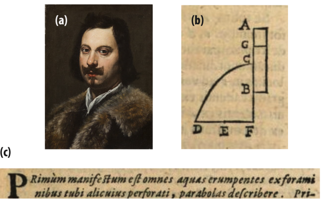
Figure 1: Torricelli’s (1644) work on the shape of horizontal jets. (a) Portrait of Torricelli by Lorenzo Lippi (ca. 1647). (b) Torricelli’s sketch of a vertical tube AB filled with water to the level G and perforated at C. CD is the parabolic trajectory of the jet. (c) Torricelli’s enunciation of the parabolic trajectories of water jets. Source for part (a): “Evangelista Torricelli”, Wikipedia, Wikimedia Foundation, 20 January 2021, https://en.wikipedia.org/wiki/Evangelista_Torricelli. Source for parts (b) and (c): https://books.google.fr/books?id=UQsOAAAAQAAJ.

Why revisit now the nearly 400 year-old question of the shape of horizontal jets? Our renewed interest in this problem began with a surprising observation in a teaching laboratory setup designed to illustrate the properties of Poiseuille flow. The working fluid is mineral oil, which is pumped through a long (6 m) pipe of inner radius 9.5 mm equipped with pressure sensors at fixed intervals. The flowing oil exits the downstream end of the pipe into a transparent air-filled chamber, whence it is recycled back to the upstream end. In view of Torricelli’s well-known result, we expected the jet exiting the pipe to have a parabolic trajectory. What we saw instead was the complex structure shown in fig. 2. The initially round jet rapidly splits into a primary jet above and a smaller secondary jet below with a thin fluid curtain connecting them. We baptized this phenomenon “Torricelli’s curtain” in honor of Torricelli’s seminal contributions to our understanding of horizontal liquid jets.

We soon discovered that Torricelli’s curtain was not confined to our laboratory. The phenomenon can be seen in the pedagogical movie“Turbulence” of the National Committee for Fluid Mechanics Films (http://web.mit.edu/hml/ncfmf.html) when an increase in the liquid viscosity causes the flow to become laminar. It can also be found in Nature. Fig. 3 shows an example of what volcanologists call a ‘firehose’: an initially horizontal jet of molten lava falling into the ocean. The primary jet is visible as a band of darker red just below the upper extremity of the curtain.

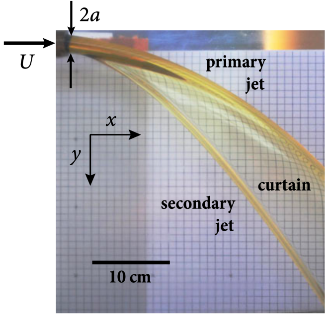
Figure 2: Structure of Torricelli’s curtain. A jet of mineral oil is ejected horizontally at mean speed $U=0.97$ m s^-1 from a 6 m long pipe with inner radius $a=9.5$ mm. The initial jet splits into a primary jet above and a smaller secondary jet below with a thin fluid curtain between them. For typical horizontal and vertical cross-sections of the whole structure see fig. 13.

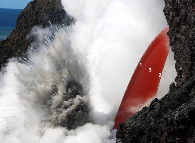
Figure 3: A natural example of Torricelli’s curtain, formed by a horizontal jet of molten lava on the flank of Kilauea volcano, Hawaii on 28 January 2017. The distance from the outlet to the sea surface is about 28 m. The numbers 1, 2 and 3 indicate the primary jet, the secondary jet, and the curtain, respectively. Public domain source: https://www.usgs.gov/media/images/open-lava-stream-continues-ocean-entry. Credit: U.S. Geological Survey, Department of the Interior/USGS.

With its two jets connected by a thin sheet, Torricelli’s curtain obviously involves separate pieces with different dynamics. The literature on both jets and sheets is immense, and a complete survey would require a separate paper. Instead, to focus the discussion we concentrate on the aspects most relevant to our work: steady axisymmetric laminar capillary jets exiting long pipes at high Reynolds number $Re$, and planar fluid sheets. Finally, we briefly survey past experimental work on buoyant jets injected horizontally into a quiescent fluid with a similar viscosity, a system that displays some striking similarities to Torricelli’s curtain.

All beginning students of fluid mechanics know that steady laminar flow in a long pipe has a parabolic (Poiseuille) velocity profile with zero velocity but finite shear stress at the pipe’s inner wall. The maximum velocity at the center of the pipe is twice the mean velocity $U$. When the liquid exits the pipe into air, the boundary condition on its outer surface changes abruptly from one of zero velocity to one of zero shear stress. In the absence of gravity and surface tension, the resulting mismatch of the shear stress between the surface and the interior is gradually erased by radial viscous diffusion, resulting in the establishment of a uniform (plug flow) profile across the jet. The far-field velocity $U_{\infty}=(4/3)U$ and radius $a_{\infty}=(\sqrt{3}/2)a$ of the jet are determined by the requirements of conservation of volume flux and momentum flux. This plug flow is established at a downstream distance $x\approx 0.25aRe$, where $Re=Ua/\nu$ is the Reynolds number.

At distances $x\ll 0.25aRe$, radial viscous diffusion is confined to a thin boundary layer of thickness $\delta(x)\ll a$ adjoining the surface of the jet, and has not yet been influenced by the jet’s finite radius. The structure of the boundary layer can therefore be treated as a two-dimensional problem of parabolic type with an outer boundary condition of constant shear $\dot{\gamma}$ given by the near-wall Poiseuille velocity profile. This problem was solved by Goren [3], who found a self-similar solution in which $\delta\sim(\nu x/\dot{\gamma})^{1/3}$. Goren [4] determined the shape of an axisymmetric jet far downstream by linearizing the Navier-Stokes equations about the jet’s final uniform state at $x/(aRe)\to\infty$. Subsequent studies considered vertical jets subject to axial gravity and (in most cases) surface tension. Examples include Duda and Vrentas[5] and Tsukiji and Takahashi[6], who transformed the boundary-layer form of the Navier-Stokes equations to streamline coordinates and solved them numerically to obtain the structure of the jet at all distances $x/(aRe)$. Philippe and Dumargue[7] used matched asymptotic expansions to obtain a semi-analytical solution for the jet structure, but did not consider the effect of surface tension. Oguz[8] solved the boundary-layer equations for an axisymmetric jet without surface tension using eigenfunction expansions and a Galerkin numerical method. Finally, in the context of a stability analysis Sevilla[9] determined the steady state of a high-$Re$ capillary jet using a numerical method of lines due to Gordillo et al.[10], which we too shall use in the sequel.

Turning to vertically flowing fluid sheets, we first note a seminal contribution of G. I. Taylor, who in the Appendix to Brown[11] derived a one-dimensional equation for the steady-state velocity of a falling liquid sheet governed by a balance of gravity, inertia and extensional viscous forces. Taylor derived his equation assuming that the velocity was constant across the sheet (plug flow). The equation was later generalized to include the effects of surface tension and nonstationarity [12, 13]. For our purposes, the most interesting phenomena connected with liquid sheets are those that occur near a free edge retracting under the influence of surface tension. Taylor[14] and Culick[15] considered the retraction of the edge of an effectively inviscid liquid sheet with thickness $h$ in the absence of gravity. By balancing surface tension and inertia, they found that the velocity of retraction is $U_{tc}=(2\gamma/\rho h)^{1/2}$ where $\gamma$ is the coefficient of surface tension and $\rho$ is the density. Keller[16] and Keller et al.[17] analyzed the shape of the growing rim on the edge of a retracting inviscid sheet and found it to be a cylinder whose radius increases as the square root of the time. Brenner and Gueyffier[13] solved numerically the one-dimensional thin-sheet equations mentioned previously. They found three different regimes depending on the Ohnesorge number $Oh=\nu(\gamma h/\rho)^{-1/2}$ and the Reynolds number $Re_{f}=VL/\nu$, where $L$ is the lateral extent of the sheet perpendicular to its edge. Both regimes with $Re_{f}\gg 1$ show the formation of a growing rim, with inward-propagating capillary waves when $Oh\ll 1$. Song and Tryggvason[18] and Sünderhauf et al.[19] solved the full two-dimensional Navier-Stokes equations in a thin sheet geometry to investigate rim formation. Both studies found that for $Oh\ll 1$ there is a growing quasi-cylindrical rim with inward-propagating capillary waves. Roche et al.[20] studied experimentally the shape of the hole downstream of a needle piercing a vertically flowing liquid curtain, and found good agreement with a theoretical model including the effect of surface tension acting on the rim. Savva and Bush[21] performed a theoretical and numerical study of viscous sheet retraction and deduced new analytical expressions for the retraction speed at rupture and the evolution of the maximum sheet thickness. Gordillo et al.[22] presented both two-dimensional and one-dimensional numerical solutions for retracting sheets, and determined an analytical solution of the one-dimensional equations that is valid in the asymptotic limit of large times. This is also an appropriate place to mention recent theoretical work by Benilov [23] on the related problem of a two-dimensional liquid curtain with strong surface tension ejected from a horizontal slot in a field of gravity.

Finally, there have been a number of experimental studies of buoyant jets injected horizontally into a quiescent ambient fluid, the source of the buoyancy being either a temperature difference [24, 25] or a compositional one [26, 27, 28, 29]. These experiments are similar to the configuration of Torricelli’s curtain in that gravity acts normal to the jet axis, but different in that the jet and the ambient fluid have comparable viscosities and no surface tension. In the context of our work the observations of Arakeri et al.[26] are particularly noteworthy. These authors performed their experiments by injecting pure water jets into denser brine solutions, so that the effective gravitational force is directed upwards. They observed that in many cases the jet bifurcated into a primary jet and a rising “plume” in the form of a thin sheet parallel to the flow direction. In fact, Fig. 8 of Arakeri et al.[26] shows a shadowgraph image that looks very much like an upside-down version of Torricelli’s curtain, with primary and secondary jets connected by a (presumably) much thinner vertical sheet of the same fluid. The observations of Arakeri et al.[26] were broadly confirmed by subsequent work [27, 28, 29].

II Dimensional analysis

As a prelude to our subsequent investigations, we use dimensional analysis to determine the dimensionless groups governing Torricelli’s curtain. The parameters of the experiment are the fluid density $\rho$, the kinematic viscosity $\nu$, the coefficient of surface tension $\gamma$, the pipe radius $a$, the mean exit velocity $U$, and the gravitational acceleration $g$. Of these six parameters, three have independent dimensions. Buckingham’s $\Pi$-theorem then tells us that three independent dimensionless groups can be formed from the six dimensional parameters. To help us choose the definitions of these groups, we note two facts. First, a typical experiment consists in varying $U$ for fixed values of the other dimensional parameters. This suggests that $U$ ought to appear in only one dimensionless group, which we choose to be the Reynolds number

$$Re=\frac{Ua}{\nu}$$ (1)

which measures the ratio of inertia to viscous forces. The second fact is that the curtain can be considered to be due to gravity acting on a jet that would otherwise have been horizontal and axisymmetric. This suggests that $g$ should appear in only one dimensionless group. We choose this group to be the ratio of two characteristic length scales. The first is the ‘Dean length’ $L_{D}$, the distance from the pipe exit at which a fluid particle moving with a horizontal speed $\sim U$ has fallen a distance $\sim a$ under gravity. Assuming a ballistic (parabolic) trajectory, we find

$$L_{D}=U(a/g)^{1/2}.$$ (2)

The second lengthscale $L_{\nu}=aRe$ is the distance from the pipe exit at which radial viscous diffusion over a length $\sim a$ has occurred. Our second dimensionless group is thus the ‘Dean number’ $De=L_{\nu}/L_{D}$, or

$$De=\left(\frac{a^{3}g}{\nu^{2}}\right)^{1/2}.$$ (3)

The third dimensionless group measures the effect of surface tension, and should contain neither $U$ nor $g$. This group is the Laplace number

$$La=\frac{\gamma a}{\rho\nu^{2}}\equiv\frac{(\gamma/a)(\rho U^{2})}{(\rho\nu U/a)^{2}}.$$ (4)

As (4) shows, $La$ can be interpreted as a characteristic value of the surface tension force times inertia divided by the square of the viscous force.

A fourth dimensionless group that we shall have occasion to use is the Weber number

$$We=\frac{\rho aU^{2}}{\gamma}$$ (5)

which measures the ratio of inertia to surface tension. It is not independent of the three groups defined previously because $We=Re^{2}/La$.

III Laboratory experiments

III.1 Experimental setups

We used two experimental setups. The first (Setup 1) is the teaching setup built by Plint & Partners Ltd. (Deltalab) for the analysis of Poiseuille flow that we mentioned in the Introduction. The working fluid is mineral oil (Total Azolla ZS22) with dynamic viscosity $\eta=0.039$ Pa s, density $\rho=860$ kg m^-3, and surface tension coefficient $\gamma=0.037$ N m^-1.

In order to be able to change the working fluid and pipe radius and to make local measurements of the curtain thickness, we built a second setup (Setup 2). This involved a 1.2 m long pipe with inner radius $a=5.5$ or 8.5 mm, through which fluid is forced by a centrifugal pump. The jet/curtain falls into a large tank whence it is pumped back to the reservoir supplying the pipe. The flow rate is controlled by adjusting the frequency of the pump. The working fluids were water/glycerine mixtures, water/glucose syrup mixtures, and silicone oil. At 25^∘C the silicone oil had $\rho=960$ kg m^-3 (decreasing with temperature at a rate of 1 kg m^-3 per K) and $\gamma=0.0207$ N m^-1. Its kinematic viscosity was about $3\times 10^{-5}$ m² s^-1 and decreases with temperature by about 1% per K. Viscosities were measured with an Anton Paar MCR 501 rheometer and surface tension with a Kruss DSA30 tensiometer.

Each of the two experimental setups has shortcomings that should be kept in mind. The main disadvantage of Setup 1 is that it cannot be disassembled, making it impossible to change the pipe or the working fluid. Moreover, the fluid is ejected into a closed chamber that prevents access to the curtain. In Setup 2, there is a small (amplitude 0.1 mm) oscillation of the pipe transmitted from the pump through the hoses. When the curtain is very thin, the oscillation leads to the formation of bubbly surfaces alternately on the two sides. A second disadvantage is that the temperature of the liquid increases as passes repeatedly through the pump, changing its viscosity and modifying the flow rate. Finally, the flow rate is not perfectly constant on shorter time scales, and oscillates with a typical frequency $<1$ Hz. Consequently, the curtain moves a little in its own plane, typically by about 1 cm in $x$.

III.2 Observations

We begin by using Setup 1 to examine how the morphology of the curtain depends on the Reynolds number $Re$. Fig. 4 shows the shape of the curtain for five values of $Re$. All five experiments have $De=58$ and $La=160$. As $Re$ increases, both the primary and secondary jets become more horizontal, as one would expect from purely ballistic considerations. For $Re\geq 180$, the primary and secondary jets move progressively further away from each other with increasing distance downstream. For $Re=120$ (fig. 4a), by contrast, the two jets first diverge and then begin to approach each other.

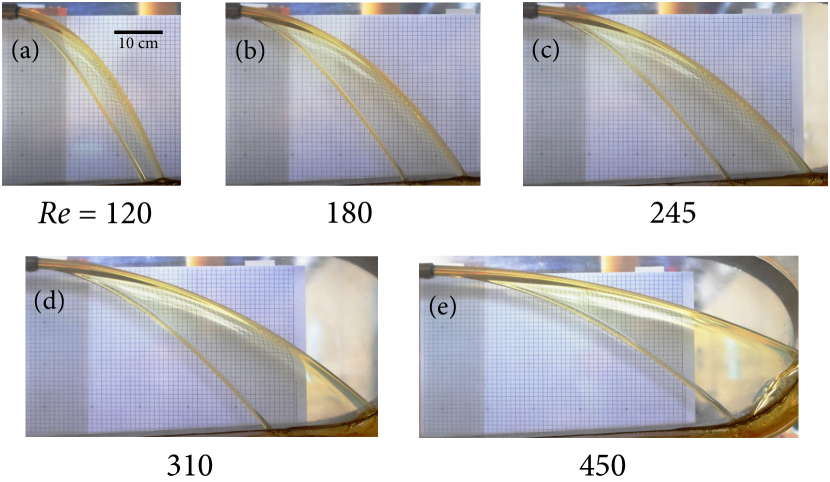
Figure 4: Shape of the curtain observed in Setup 1 as a function of the Reynolds number $Re=$ (a) 120, (b) 180, (c) 245, (d) 310 and (e) 450. The approximate values of the Dean and Laplace numbers are $De=58$ and $La=160$. The grid squares in the background are 1 cm across.

The approach of the primary and secondary jets in fig. 4a raises the question of what would happen further downstream if the jets had not been blocked by the bottom of the transparent chamber. This can be explored using experiments with setup 2 and diluted glucose syrup, for which the large surface tension effect pulls the secondary jet strongly upwards towards the primary one. Fig. 5 shows a close-up view of one such experiment with $Re=1360$, $De=160$ and $La=4300$. The approaching primary and secondary jets eventually collide to form a ‘fluid chain’ [30].

At large flow rate and for $a=8.5$ mm in Setup 2 the film grows quite thin far downstream from the pipe exit and becomes unstable. Sinuous waves of rapidly growing amplitude are observed, reminiscent of the flutter instability studied recently by Dighe and Gadgil[31]. Further study of this instability is beyond the scope of this paper.

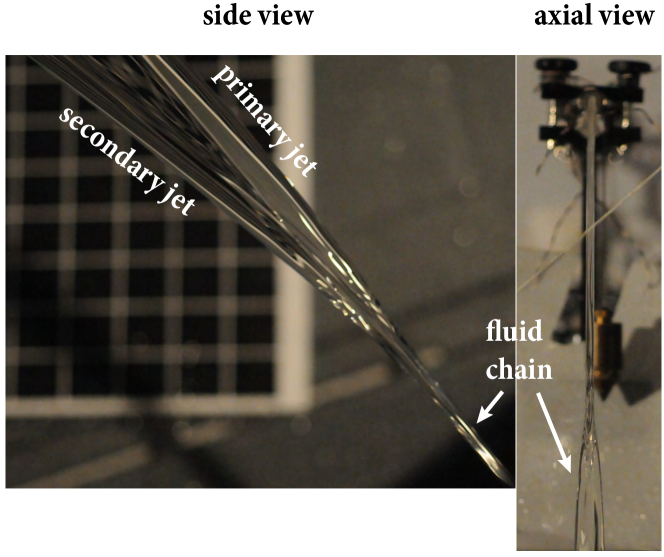
Figure 5: Fluid chain resulting from the collision of the primary and secondary jets. The experiment is performed using Setup 2 with $a=5.5$ mm and diluted glucose syrup as the working fluid. The values of the dimensionless groups are $Re=1360$, $De=160$ and $La=4300$. The grid squares in the background are 2 cm across.

III.2.1 Rescaling of the curtain shape

Next, we ask whether the trajectories of the primary and secondary jets can be rescaled to yield universal curves. Fig. 6a shows 8 profiles of the upper boundary (top) and the lower boundary (bottom) of the primary jet for different values of the mean exit velocity $U$, obtained using Setup 2 with silicone oil and a pipe having $a=5.5$ mm. For these experiments $Re\in[160,330]$, $De=40$ and $La=120$.

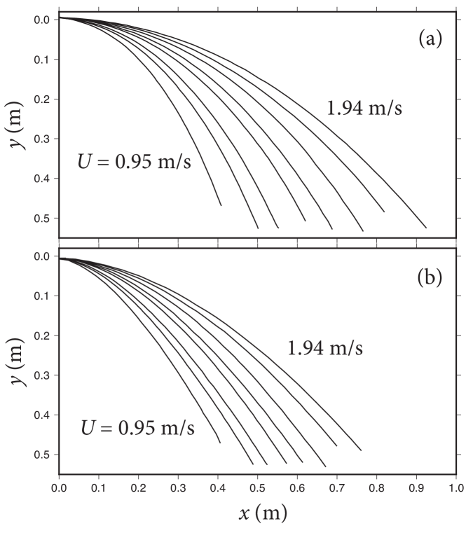
Figure 6: Profiles of (a) the upper boundary of the primary jet and (b) the lower boundary of the secondary jet for different values of the mean exit velocity $U$, obtained using Setup 2 with silicone oil and a pipe having $a=5.5$ mm. The corresponding dimensionless parameters are $Re\in[160,330]$, $De=40$ and $La=120$.

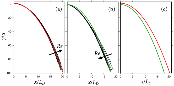
Figure 7: Rescaled curves from fig. 6. Parts a) and b) correspond to parts a) and b) of fig. 6. The red and green curves are parabolas that best fit the experimental data, and correspond to $U_{eff}/U$ = 1.43 and 1.28, respectively. The arrows show the sense of increasing Reynolds number $Re$. Part (c) shows the two parabolas together to facilitate comparison.

To rescale the curves in fig. 6, we choose new scaled variables $Y=y/a$, $X=x/L_{D}$, where $L_{D}$ is the Dean length defined by (2). Fig. 7 shows the rescaled versions of the curves of fig. 6. All the data collapse onto a universal curve for $X<10$. For larger values of $X$ significant differences among the scaled curves are evident, especially for the lower rim (fig. 7b).

Proceeding in a Torricellian way, we now determine the parabola that best fits the curves in fig. 7. The equation for the parabolic trajectory of a particle having an effective horizontal velocity $U_{eff}$ and initial position $y=\mp a$ is

$$y=\mp a+\frac{gx^{2}}{2U^{2}_{eff}}\quad\to\quad Y=\mp 1+\frac{1}{2}\left(\frac{U}{U_{eff}}\right)^{2}X^{2},$$ (6)

where the plus and minus signs correspond to the top and bottom of the jet at the pipe exit. Using a simple least-squares fit to the data in fig. 7 we obtain the parabolas shown by the red and green lines in that figure. The parabolic fit to the data is good for the upper boundary (fig. 7a) but less good for the lower boundary (fig. 7b). The best-fitting parabolas for the upper and lower boundaries have $U_{eff}/U=1.43$ and 1.28, respectively. Note that $U_{eff}/U$ must be less than 2 because the fastest particles on the pipe axis have velocity $2U$.

Fig. 8 is the same as fig. 7 but for a suite of 17 experiments with a larger pipe radius $a=8.5$ mm. The upper boundary of the primary jet (fig. 8a) is again well fit by a parabola with $U_{eff}/U=1.46$, nearly the same value as for the parabola in fig. 7a. By contrast, the data for the lower boundary of the secondary jet (fig. 8b) clearly do not collapse onto a universal curve, and are consequently poorly fit by a parabola (green line corresponding to $U_{eff}/U=1.04$) that is shown only for completeness. The secondary jet is clearly strongly affected by $Re$, being lower (in this dimensionless representation) when $Re$ is larger.

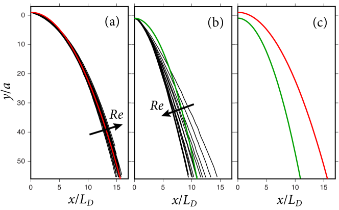
Figure 8: Same as parts (a)-(c) of fig. 7, but for 17 experiments with $a=8.5$ mm. The corresponding dimensionless parameters are $Re\in[150,480]$, $De=80$ and $La=200$. The best-fitting parabolas (red and green lines) have $U_{eff}/U=1.46$ and 1.04, respectively.

III.2.2 Thickness measurements

The thickness of the curtain in the $z$-direction (into the plane of the page) is measured in setup 2 using a local optical probe (Chromapoint from STIL, http://point.stil-sensors.com/?lang=EN). Incident white light traverses a chromatic lens and the reflected light is analysed. The color of the reflected light gives the distance to the interface. With a transparent liquid two resolved peaks can be observed in the spectrogram and, if the optical index of the liquid is known, the film thickness $h(x,y)$ can be measured with a 10 $\mu$m resolution and at a 1 kHz acquisition frequency. The optical probe can be translated vertically or horizontally by an $x$-$y$ carriage. Unfortunately, thicknesses in the two jets cannot be measured with this method as the slopes of the interfaces are too large there. We note that the background grids visible in figures 2, 4, 5 and 10 are solely for calibration of distances in the $x$- and $y$-directions, and play no role in the measurements of the curtain thickness.

The black dots in Figure 9 show (a) vertical and (b) horizontal profiles of the thickness measured in a laboratory experiment with $Re=380$, $De=80$ and $La=194$. The thickness of the sheet in between the two jets increases in $x$ and decreases in $y$. The solid and dashed lines show theoretical predictions that will be discussed later.

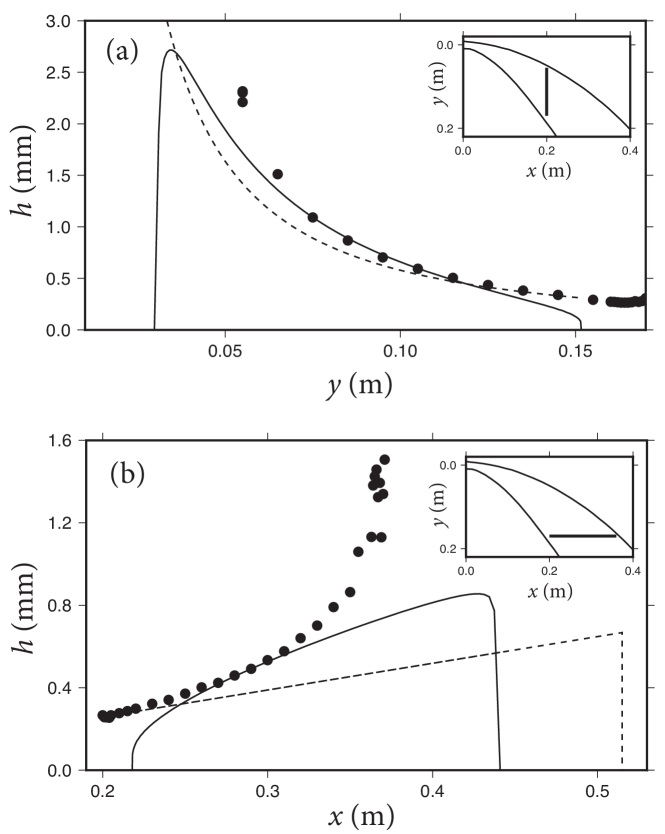
Figure 9: Black dots: vertical (a) and horizontal (b) profiles of the curtain thickness $h$ measured in a laboratory experiment with $Re=380$, $De=80$ and $La=194$. The locations of the profiles are shown in the insets. Dashed and solid lines are the predictions (12) and (22) of the simple and corrected ballistic models, respectively.

III.2.3 Dean recirculation

Using setup 2, we were able to inject dye into the upper side of the jet close to its exit from the pipe. The dye was observed by eye to follow spiral trajectories down the jet, corresponding to a secondary flow comprising two cells having longitudinal vorticity of opposite sign. Such behavior is reminiscent of Dean recirculation in curved pipes [32]. We will have more to say about Dean recirculation below in § V.2.

IV Theoretical analysis

IV.1 Simple ballistic model

To start simply, we present a zeroth-order model for the curtain by supposing that fluid particles exiting the pipe do not interact with one another in any way. This amounts to ignoring viscosity and surface tension. Each particle therefore describes a parabolic trajectory corresponding to its initial velocity of exit from the pipe. The exit velocity $u_{x}(r)$ as a function of the radius $r$ across the pipe is that of a developed Poiseuille flow, and is

$$u_{x}(r)=Uf_{0}(r),\quad f_{0}(r)=2\left(1-\frac{r^{2}}{a^{2}}\right).$$ (7)

The equations governing the trajectories are the ballistic equations $\dot{x}=u_{x}(r)$ and $\ddot{y}=g$, where dots denote derivatives with respect to the time $t$. Solving these and eliminating the parameter $t$, we obtain

$$y=r+\frac{gx^{2}}{2u_{x}(r)^{2}}.$$ (8)

The red and green dashed lines in Figure 10 show the trajectories (8) with $r=0$ (red) and $r=a$ (green), for an experiment using Setup 1. The red dashed line is a parabola corresponding to the maximum exit velocity $u_{x}(0)=2U$. It follows reasonably closely the trajectory of the primary jet, but is systematically too high. The vertical green dashed line is the (degenerate) parabolic trajectory corresponding to the minimum exit velocity $u_{x}(a)=0$. It bears no relation to the trajectory of the secondary jet, indicating that a simple ballistic model is not valid for particles exiting the pipe near its wall.

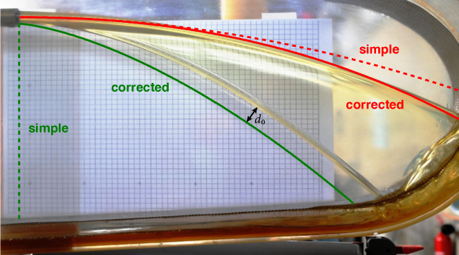
Figure 10: Trajectories predicted by the simple (dashed lines) and corrected (solid lines) ballistic models, compared with an experiment with $Re=450$, $De=64$ and $La=200$. Red lines are trajectories of particles exiting the pipe at the center $y=0$, and green lines are for particles exiting at the bottom $y=a$. The black double-headed arrow indicates a typical difference $d_{0}$ between the prediction of the corrected ballistic model and the observed lower extremity of the secondary jet.

The expression (8) for the trajectories allow us to derive an expression for the thickness $h(x,y)$ of the curtain. We sketch the derivation here to illustrate the basic idea, which will be applied to a more realistic model in the next section. For simplicity, we neglect the finite radius of the pipe, which is equivalent to making a ‘far-field’ assumption $(x,y)\gg a$. The equation (8) for the trajectories now becomes

$$y(x,r)=\frac{gx^{2}}{2u_{x}(r)^{2}}.$$ (9)

Denoting by $h_{1}$ the thickness predicted by the simple ballistic model, we equate the flux of fluid exiting the pipe through an annulus of area $2\pi r\mathrm{d}r$ to the flux crossing a vertical plane at some fixed downstream position $x$. This requires

$$2\pi ru_{x}(r)\mathrm{d}r=h_{1}u_{x}(r)\mathrm{d}y,$$ (10)

where $\mathrm{d}y$ is the infinitesimal height of the portion of the curtain through which fluid from the annulus of width $\mathrm{d}r$ passes. Rearranging (10), we obtain

$$h_{1}=2\pi r\left(\frac{\partial y}{\partial r}\right)^{-1}.$$ (11)

Differentiating (9) with respect to $r$ and substituting the result into (11), we obtain

$$h_{1}(x,y)=\frac{\pi a^{2}}{4U}\left(\frac{g}{2y^{3}}\right)^{1/2}x.$$ (12)

Introducing $H_{1}=h_{1}/a$ the foregoing equation can be written in dimensionless form as

$$H_{1}(X,Y)=\frac{\pi}{4\sqrt{2}}\,Y^{-3/2}X.$$ (13)

Eqn. (13) predicts that for constant $Y$ the curtain has a thin ‘wedge’ shape with $H_{1}\propto X$. We shall compare the prediction (12) with observations after introducing a corrected ballistic model that accounts for the effects of viscosity.

IV.2 Corrected ballistic model

In this section we propose a corrected ballistic model for the morphology of the jet. The idea is to model the flow as the composition of two components: the axisymmetric flow within a steady horizontal jet in the zero-gravity limit, and a downward vertical velocity due to free fall under gravity. The model differs from the simple ballistic model of the previous section by accounting for the effects of viscosity on the axisymmetric horizontal jet.

The first task is to determine the steady axisymmetric flow in a horizontal jet in the absence of gravity. Figure 11 shows a definition sketch of the jet. The velocity within the jet is $\mathbf{u}=u_{r}\mathbf{e}_{r}+u_{x}\mathbf{e}_{x}$, where $\mathbf{e}_{r}$ and $\mathbf{e}_{x}$ are unit vectors in the directions indicated by subscripts. The radius of the jet is $R(x)$, and the radius of the pipe is $a$.

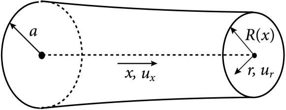
Figure 11: Definition sketch of a steady axisymmetric horizontal jet in the absence of gravity. The axial and radial components of the velocity are $u_{x}$ and $u_{r}$, respectively. The radius of the nozzle is $a$, and the radius of the jet is $R(x)$, where $x$ is the distance from the nozzle.

Following Sevilla[9], the governing equations in the boundary-layer approximation are

$$r\frac{\partial u_{x}}{\partial x}+\frac{\partial}{\partial r}(ru_{r})=0,$$ (14)

$$u_{x}\frac{\partial u_{x}}{\partial x}+u_{r}\frac{\partial u_{x}}{\partial r}=\frac{\gamma R^{\prime}}{\rho R^{2}}+\frac{\nu}{r}\frac{\partial}{\partial r}\left(r\frac{\partial u_{x}}{\partial r}\right)$$ (15)

where $\gamma$ is the coefficient of surface tension and $R^{\prime}=\mathrm{d}R/\mathrm{d}x$. Eqn. (14) is the continuity equation, and (15) is the axial momentum equation. The radial momentum equation in the boundary-layer approximation simply states that the pressure does not vary across the jet. This allows one to set the pressure everywhere equal to the capillary pressure $p_{c}$. Because $R(x)$ is assumed to vary slowly over a length scale $aRe$, the capillary pressure gradient $-\mathrm{d}p_{c}/\mathrm{d}x\equiv\gamma R^{\prime}/\rho R^{2}$ is due only to the azimuthal curvature of (circular) jet cross-sections, and does not take into account the second (and much smaller) principal curvature in the axial direction.

Equations (14) and (15) must be solved subject to the conditions

$$u_{x}(0,r)=Uf_{0}(r),\quad f_{0}=2(1-r^{2}/a^{2}),$$ (16)

$$\frac{\partial u_{x}}{\partial r}(x,a)=0,$$ (17)

$$u_{r}(x,0)=\frac{\partial u_{x}}{\partial r}(x,0)=0,$$ (18)

$$u_{r}(x,a)=R^{\prime}u_{x}(x,a).$$ (19)

Condition (16) states that the flow exiting the nozzle $x=0$ has a parabolic (Poiseuille) profile with a mean exit velocity $U$. Condition (17) states that the outer surface of the jet is free of shear traction. Conditions (18) state that the radial velocity and the radial derivative of the axial velocity vanish on the axis $r=0$ of the jet. Finally, condition (19) is the kinematic condition on the jet’s outer surface.

We now nondimensionalize the foregoing boundary-value problem by introducing new dimensionless variables $r/a$, $x/(aRe)$, $u_{x}/U$, and $u_{r}Re/U$. The only two dimensionless groups that appear are then $Re$ and $We$. We solved the dimensionless problem numerically using the method of lines outlined by Gordillo et al.[10]. Of primary interest for our corrected ballistic model are the axial velocities $u_{x}(x,0)$ and $u_{x}(x,a)$ along streamlines corresponding respectively to the central axis $r=0$ and to the outer surface $r=a$ of the jet. These are shown in Figure 12 for $We=10$ (dashed lines) and 1000 (solid lines). Fluid on the outer surface accelerates rapidly, and fluid on the axis decelerates more slowly, both tending towards the same final plug flow velocity $(4/3)U$. This behavior is due to radial viscous diffusion of vorticity consequent upon the sudden change in the outer boundary condition from rigid to free when the jet exits the pipe. The dashed and solid curves in Figure 12 are almost identical, indicating that surface tension plays only a minor role in the dynamics of horizontal jets when $We\gg 1$.

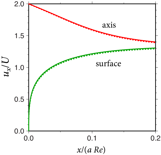
Figure 12: Velocities $u_{x}(x)$ on the axis (red lines) and the outer surface (green lines) of an axisymmetric horizontal jet in the absence of gravity, for $We=10$ (dashed lines) and 1000 (solid lines).

IV.2.1 Particle trajectories

The horizontal velocities shown in Figure 12 can now be transformed into nominal particle trajectories by adding a vertical component of motion corresponding to free fall. Let $y$ be the downward vertical coordinate with origin at the center of the pipe. The horizontal velocity of the axisymmetric jet is

$$u_{x}=Uf\left(\zeta,r\right),\quad\zeta=\frac{x}{aRe}$$ (20)

where $r\in[0,a]$ is the radial coordinate across the pipe. The function $f(\zeta,0)$ is the upper curve in Figure 12, and $f(\zeta,a)$ is the lower curve in that figure. We now combine (20) with the free fall equation $\ddot{y}=g$, obtaining

$$y(x,r)=r+\frac{g}{2}\left[\frac{a^{2}}{\nu}I(x,r)\right]^{2},\quad I(x,r)=\int_{0}^{x/(aRe)}\frac{\mathrm{d}\zeta}{f(\zeta,r)}.$$ (21)

The dimensionless integral $I$ is just the time required for a particle starting at a radius $r$ to travel a distance $x$, measured in units of the characteristic viscous diffusion time $a^{2}/\nu$.

The red and green solid lines in Figure 10 show the trajectories predicted by the corrected ballistic model for the reference experiment. The solid red line now follows closely the position of the primary jet, indicating that the corrected ballistic model is accurate for that jet. The solid green line staring at $y=a$ is also much closer to the position of the secondary jet than was the prediction of the simple ballistic model (dashed green line). Nevertheless, the corrected ballistic model still predicts that the lower extremity of the secondary jet lies substantially lower than its true position. There are at least two possible reasons for this discrepancy. One is that the model envisions purely radial viscous diffusion in an axisymmetric jet, which is no longer a valid assumption when the lower part of the jet has become strongly non-axisymmetric. A second reason is the neglect in the model of the surface tension-driven retraction of the secondary jet and the attached thin fluid curtain, which counteracts their tendency to move downwards under gravity. This effect will be estimated shortly in § IV.2.3.

IV.2.2 Curtain thickness

The corrected ballistic model allows us to predict the curtain’s thickness $h_{2}(x,y)$ as a function of position. Balancing fluxes as we did in the previous section, we obtain

$$2\pi rUf_{0}(r)\mathrm{d}r=u_{x}(x,r)h_{2}\mathrm{d}y\quad\to\quad h_{2}(x,r)=2\pi r\frac{f_{0}(r)}{f(\zeta,r)}\left(\frac{\partial y}{\partial r}\right)^{-1}$$ (22)

where $y(x,r)$ is given by (21). Equations (21) and (22) are two parametric equations for $y(x,r)$ and $h_{2}(x,r)$ with $r$ as a parameter, and must be solved numerically. It is easy to verify that (22) reduces to the corresponding inviscid result (12) by setting $f(\zeta,r)=f_{0}(r)$ and making the far-field assumption by neglecting the first term ($=r$) on the right-hand side of (21).

We are now in a position to compare the predictions $h_{1}(x,y)$ and $h_{2}(x,y)$ of our two ballistic models with the experimental measurements shown by the black circles in fig. 9. That figure also shows (a) vertical and (b) horizontal profiles of $h_{1}$ (dashed lines) and $h_{2}$ (solid lines) for the parameters of the experiment. Both ballistic models do a reasonably good job of predicting the vertical profile (fig. 9b), including the rapid thickening for small values $y\approx 0.05$-0.06 m as the primary jet is being approached. The situation for the horizontal profile of fig. 9b is more complicated. Each ballistic model predicts well a portion of the observations at small values of $x<0.32$. However, neither model predicts the rapid increase in thickness for larger values of $x$.

IV.2.3 Effect of surface tension

We now investigate whether the discrepancy between the observed and calculated positions of the secondary jet (fig. 10) is due to the (hitherto unmodelled) effect of surface tension. To begin, we recall the expression derived by Taylor[14] and Culick[15] for the velocity $U_{tc}$ of surface tension-driven retraction of the free edge of a two-dimensional viscous sheet with constant thickness $h$:

$$U_{tc}=\left(\frac{2\gamma}{\rho h}\right)^{1/2}.$$ (23)

The formula (23) translates the balance between surface tension and inertia at the free edge. Refer now to fig. 10, in which the black double-headed arrow indicates the typical distance $d_{0}$ between the numerically predicted and true lowermost streamlines of the secondary jet. The corrected ballistic model also predicts the travel time of a fluid particle from the pipe exit to any point on the green streamline; let $\tau_{0}$ be the travel time to the point at the base of the black double-headed arrow in fig. 10. We now ask: can the separation $d_{0}$ be accounted for by Taylor-Culick (T-C) retraction of the curtain’s free lower edge during the time $\tau_{0}$? Because we do not know the appropriate value of $h$ to use, we solve the equation $d_{0}=U_{tc}\tau_{0}$ for $h=h_{eff}$. We obtain:

$$h_{eff}=\frac{2\gamma\tau_{0}^{2}}{\rho d_{0}^{2}}.$$ (24)

The quantity $h_{eff}$ is the effective thickness of the curtain for which the T-C formula (23) predicts retraction by an amount $d_{0}$ in a time $\tau_{0}$. For the experiment of fig. 10, $d_{0}=0.032$ m and $\tau_{0}=0.20$ s, whence (24) predicts $h_{eff}=3.5$ mm. This value of $h_{eff}$ is significantly larger than the typical curtain thicknesses $h\approx 0.3$-1 mm shown in fig. 9. For such thicknesses, T-C retraction is too fast (by a factor of $\approx 3$-4) to explain the observed separation $d_{0}$ in Figure 10. However, the foregoing calculation is subject to significant uncertainty given that the T-C formula applies to an idealized inviscid two-dimensional sheet of constant thickness. Moreover, we note that in our experiments with sugar syrup, the secondary jet is strongly “pulled up” towards the primary jet, an effect that is certainly due to the large surface tension of the syrup. This observation leads us to conclude that surface tension plays an important role in determining the trajectory of the secondary jet, both for sugar syrup and (to a lesser extent) for the mineral oil used in the experiment of Figure 10.

V Direct numerical simulation

To gain further insight into the morphology and dynamics of Torricelli’s curtain, we performed a direct numerical simulation using the volume-of-fluid code Gerris Flow Solver (GFS) [33]. This code solves for the flow in a system comprising two fluid phases, oil and the surrounding air in our case. Our flow domain is a rectangular box, $0\leq x\leq 24a$, $-2a\geq y\geq 14a$, and $0\leq z\leq 4a$, where the origin is the center of the nozzle and $y$ increases downward. Because the jet has mirror symmetry across the vertical $x$-$y$ plane, we solve the problem only for the half-domain $z>0$. On the left boundary $x=0$, we impose the boundary condition (7) corresponding to developed Poiseuille flow. The two fluid phases are distinguished by values of a phase variable $T=0$ (air) and $T=1$ (oil), separated by a thin diffuse interface across which $T$ varies rapidly from 0 to 1.

Torricelli’s curtain is quite challenging to simulate numerically due to the three-dimensionality of the problem and the wide separation of lengthscales between the pipe diameter and the thinnest part of the curtain. It is therefore necessary to exploit the octree adaptive grid refinement capacity of GFS, which divides cubes at a given refinement level into eight smaller cubes. The numerical flow domain initially consisted of 24 cubes with sides equal to $4a$. We used a maximum grid refinement of a factor of $2^{8}=256$, so that the smallest cube of the refined grid has a side equal to $a/64$. At the end of our simulations, the grid comprised a maximum of $\approx 1.6\times 10^{6}$ cubes.

For our first simulation, we chose parameter values corresponding to one of our laboratory experiments with Setup 2 using silicone oil, for which the values of the dimensionless groups are $Re=480$, $De=80$ and $La=200$. We ran the simulation for a dimensional time $t=0.63$ s, which corresponds to 5.3 transit times across the length ($=24a$) of the numerical box at the mean velocity $U$. We verified that this run time was sufficient to achieve a steady state by comparing three solutions obtained using a grid refinement of $2^{7}$ for times 0.33 s, 0.46 s, and 0.58 s. The shapes of the jet at 0.33 s and 0.46 s were noticeably different, but those for 0.46 s and 0.58 s were indistinguishable.

V.1 Shape and thickness of the curtain

Figure 13a shows the thickness $h(x,y)$ of the simulated curtain. For comparison, the brick red lines show the upper and lower extremities of the primary and secondary jets measured from a photograph of the laboratory experiment. The agreement between the experiment and the numerics is acceptable for the primary jet, but poor for the secondary jet. Results were similar for other simulations for parameters corresponding to other laboratory experiments. In the Discussion below we speculate on the likely causes of the discrepancy between the numerics and the experiments; briefly, we think it is due to a difference in the effective upstream velocity boundary condition. However, we pursue the simulations here in order to obtain valuable information that is not accessible in the laboratory experiments.

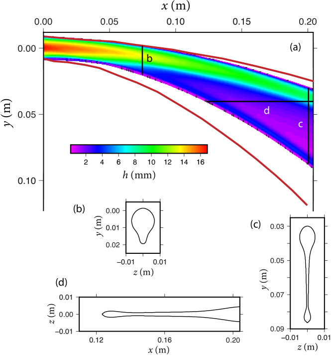
Figure 13: (a) Thickness $h(x,y)$ of a curtain simulated using Gerris Flow Solver [33] with $Re=480$, $De=80$, and $La=200$. Brick red lines are the experimentally observed extremities of the curtain for the same parameters. (b)-(d) Vertical and horizontal cross-sections of the curtain along the black lines labelled b, c and d in part (a).

We begin by examining some vertical and horizontal cross-sections of the curtain shown in fig. 13a. The locations of the cross sections are indicated by the vertical and horizontal black lines labelled b, c and d. The corresponding thickness profiles are shown in parts (b), (c) and (d) of the figure. After remaining nearly circular out to distances of a few pipe diameters, the cross-section of the curtain develops a pronounced up-down asymmetry, with a nascent curtain beneath the primary jet (profile b). By the time the fluid has reached a distance $x=0.2$ m, the initial asymmetry has developed into the now-familiar structure comprising primary and secondary jets connected by a thin curtain (profile c). The horizontal profile in part (d) shows that the thickness of the curtain between the two jets increases approximately linearly with $x$, in qualitative agreement with the predictions of the two ballistic models.

V.2 Particle trajectories and Dean recirculation

The simulations also allow us to calculate three-dimensional particle trajectories within the curtain. Because these are difficult to visualize, we instead examine the motion of a handful of material particles. Fig. 14a illustrates the motion of 13 material particles in a GFS numerical simulation with $Re=245$, $De=58$ and $La=161$. The particles are initially distributed uniformly over the circular cross-section of the jet as it exits the pipe. Fig. 14b shows five representative trajectories in the symmetry plane $z=0$ of the curtain; the progressive vertical widening of the curtain with distance downstream is evident. Finally, Fig. 14c shows the positions of the 13 material particles at the distance $x=24a$ corresponding to the right boundary of Fig. 14b. Note that the fluid in the secondary (lower) jet originates mainly from the outermost layer of the jet exiting the pipe, which flows downward around the circumference of the primary jet.

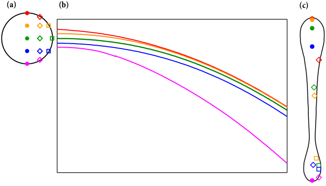
Figure 14: Trajectories of selected material particles predicted by direct numerical simulation of a curtain with $Re=245$, $De=58$ and $La=161$. (a) Distribution of 13 material particles over the cross-section of the jet exiting the pipe. (b) Selected trajectories in the symmetry plane $z=0$. (c) Positions of the 13 material particles in the curtain at the distance $x=24a$ corresponding to the right boundary of part (b).

Finally, we use our simulations to investigate the velocity field within a vertical cross-section of the jet close to the pipe, where the cross-section is still nearly circular. To make clearer the structure of the velocity field, we first subtract from it the mean vertical (downward) velocity of the section. The result is shown in fig. 15 for a section at $x=2a$ in the same numerical simulation shown in Fig. 14. The flow consists of a recirculating vortex with downward flow on the outside of the jet, together with a mirror-image vortex on the other side $z<0$ of the jet. Even though we are at a relatively short distance ($=2a$) from the pipe exit, the amplitude of the horizontal velocity $u_{z}$ is already about $\pm 8\%$ of the mean exit velocity $U$.

Recirculating vortices are prominent features of flow in curved pipes, in which context they are known as Dean vortices [32]. Such vortices are required by the conservation of angular momentum, and can be understood in terms of vortex-line tilting. When the fluid exits the pipe, the vorticity vector is everywhere azimuthal, and the vortex lines are concentric circles around the center of the pipe. As the fluid moves away from the pipe exit, the vortex lines are gradually tilted by the action of gravity. This imparts to the vorticity a small horizontal component, which must be compensated to ensure that the total horizontal component remains zero. The compensation occurs by means of an induced recirculation comprising two counterrotating Dean vortices on either side of the central symmetry plane of the jet.

To quantify the foregoing argument, we recall that the axial velocity $u_{x}(r)$ of the fluid exiting the pipe is given by (7). The vorticity associated with this velocity profile is $(4Ur/a^{2})\mathbf{e}_{\theta}\equiv\omega(r)\mathbf{e}_{\theta}$, where $\mathbf{e}_{\theta}$ is an azimuthal unit vector. Therefore $\omega\sim U/a$ because $r\sim a$. Now as the fluid moves away from the pipe exit, gravity tilts the vortex lines by a small angle $\theta(x)$. This gives rise to a small axial component of vorticity $\sim\pm(U/a)\theta$, where $\pm$ indicates that the axial component has opposite signs over the right and left halves of the jet section. This vorticity must be compensated by an axial component of vorticity $\sim\mp U_{Dean}/a$ associated with Dean recirculation, where $U_{Dean}$ is the amplitude of that recirculation. Thus we have $U_{Dean}/U\approx\theta$. To estimate $\theta$, we consider the ballistic trajectory of a particle with horizontal velocity $\approx U$, which is $y=gx^{2}/(2U^{2})$. The slope of that trajectory is $\mathrm{d}y/\mathrm{d}x=gx/U^{2}\approx\theta$. Now define $x=\xi a$, where $\xi$ is the dimensionless distance from the pipe exit. Recalling the definitions of $Re$ and $De$, we find $U_{Dean}/U\approx\xi(De/Re)^{2}$. For the case shown in fig. 15, $Re=245$, $De=58$ and $\xi=2$, which gives $U_{Dean}/U\approx 0.11$. This value is comparable to the total amplitude $U_{Dean}/U\approx 0.16$ found in the numerical simulation of fig. 15.

Figure 15: Velocity field (projected onto the section) in a vertical plane $x=2a$, for the numerical simulation shown in fig. 14. The velocity field shown does not include the mean downward velocity of the section, which has been removed.

VI Discussion

Returning to Torricelli’s discovery of the parabolic trajectory of water jets, we can now see why the simple behavior he observed is so different from the one we have investigated here. The fundamental difference between the two situations is that the velocity profile across a (turbulent) water jet issuing from a hole is nearly constant, whereas the profile across a (laminar) jet issuing from a long pipe is parabolic. In consequence, all particles in a water jet follow nearly the same ballistic (parabolic) trajectory, whereas particles issuing from a laminar flow in a pipe follow different trajectories depending on their different initial velocities. Torricelli’s curtain is therefore only observed if the flow through the pipe is laminar; as soon as it becomes turbulent, we recover the situation of a water jet issuing from a hole. The dramatic change in jet morphology that occurs at the laminar/turbulent transition is clearly visible in the NCFMF film “Turbulence” cited in the Introduction.

Our corrected ballistic model assumes that the velocity of a particle is the composition of the (dominantly horizontal) motion in an axisymmetric jet and a vertical motion due to free fall under gravity. This assumption is valid if the typical horizontal velocity $\approx U$ of the axisymmetric jet is greater than or comparable to the free-fall velocity $V$ everywhere within the ‘developing’ portion of the axisymmetric jet, i.e. before the plug-flow velocity profile has been achieved. The latter occurs at a distance $x\approx 0.25aRe\equiv x_{0}$ from the pipe exit. The characteristic free-fall velocity at this distance is $V\approx gx_{0}/U$. Using the definitions of $De$ and $Re$, we find that

$$\frac{V}{U}\leq 1\quad\mathrm{if}\quad\frac{De^{2}}{Re}\leq 4.$$ (25)

Taking the experiment of fig. 10 as an example, we find $De^{2}/Re=9.2$, or a factor 2.3 larger than the criterion (25). Thus we conclude that the experiment of fig. 10 does not quite satisfy our velocity composition assumption. By contrast, the assumption is strongly violated for the experiments with $Re=120$ and 180 in fig. 4.

A question raised by our work is whether the distinct secondary jet we observe is a consequence of surface tension. Our experiments cannot by themselves answer this question because surface tension cannot be eliminated in our setups. By contrast, the effect of surface tension is negligible in experiments on miscible buoyant jets injected horizontally into a fluid of comparable viscosity [26, 29]. Because a secondary jet is clearly seen in a number of these experiments, we conclude that surface tension is not a necessary condition for its existence. However, if surface tension is present it will of course influence the position of the secondary jet by causing Taylor-Culick retraction of the jet’s free edge.

Figure 13 has shown that our direct numerical simulations of Torricelli’s curtain disagree with experiment in at least one important respect: the vertical extent of the curtain is significantly smaller in the simulations than in reality. A possible reason for this is limited numerical resolution. In our most highly resolved simulations, the smallest cube in the grid has dimension $a/64$, or 0.13 mm for Setup 2 with $a=8.5$ mm. For typical curtain thicknesses $h=0.5$-1.0 mm measured using this setup (fig. 9), there are therefore 2 to 4 grid cubes across the half-thickness $h/2$, which should be adequate to resolve the structure of the curtain. To verify this, we compared a simulation with resolution $a/64$ to one with lower resolution $a/32$, and found that the vertical extent of the curtain was the same to within a few percent.

A second possible reason for the discrepancy is that our simulations were not run long enough to reach steady state. However, this is unlikely in view of the test we reported previously in which we found that simulations run for different times gave indistinguishable results.

A final possible reason for the disagreement between simulation and experiment is a difference in the effective upstream boundary condition at the pipe exit. In the simulations, this condition is a radially symmetric parabolic velocity profile corresponding to developed Poiseuille flow in the pipe. In the laboratory, however, this simple condition may not be realized. Evidence for this is the non-horizontality of the jet just after its exit from the pipe, clearly visible in fig. 2. This feature may be due to retroaction of the external low-pressure ambient air on the fluid in the pipe just upstream of the exit, modifying the parabolic profile and imparting a downward component to the exit velocity. Such a downward component would have a stronger influence on the relatively slow-moving secondary jet than on the primary jet, which is consistent with fig. 13. In summary, we believe that different effective boundary conditions are the most likely explanation for the discrepancy between experiment and simulation evident in fig. 13.

Torricelli’s curtain has remarkable similarities with the flow in curved rigid pipes[34, 32]. To investigate flow in a pipe whose axis has a radius of curvature $R$, one first seeks a scaling for the axial arclength coordinate $s$ and the transverse (in-section) velocity $\mathbf{u}_{trans}$ that renders the centrifugal force terms in the transverse momentum equations comparable in magnitude to the inertial and viscous terms. The scaling that does this is $s\sim a\delta^{-1/2}$, $\mathbf{u}_{trans}\sim\delta^{1/2}U$ where $\delta=a/R$. Now for a free horizontal jet whose curvature is due to gravity, the ballistic equation $y=gx^{2}/(2U^{2})$ implies $R=U^{2}/g$ at $x=0$. The axial length scale $a\delta^{-1/2}$ then takes the form $U(a/g)^{1/2}$, which is just the expression for the Dean length $L_{D}$ that we introduced in § II. Furthermore, the Dean number for a curved pipe is defined as $De=\delta^{1/2}Re$, which for our problem turns out to be $De=(a^{3}g/\nu^{2})^{1/2}$. The expression $De=\delta^{1/2}Re$ shows that the Dean number is an effective or ‘reduced’ Reynolds number for flow in a curved pipe. In fact, in the so-called ‘loosely coiled pipe’ limit $\delta\ll 1$, $De$ is the only dimensionless parameter that appears in the rescaled Navier-Stokes equations, implying that all curved pipe flows with the same value of $De$ are dynamically similar[35]. For our experiments using Setup 1, $\delta\equiv ag/U^{2}\in[0.020,0.52]$, which spans the range from the loosely coiled (e.g. fig. 4e with $\delta=0.02$) to the strongly coiled limits (e.g. fig. 4a with $\delta=0.20$). Of course a liquid curtain differs from classical curved pipe flow in important respects: the outer surface of the fluid is free and deformable, and surface tension plays an important role in the dynamics. Nevertheless, it is illuminating to regard Torricelli’s curtain as a free-surface curved pipe flow problem in which the shape of the ‘pipe’ must be determined as part of the solution.

In closing, we return to the lava firehose observed at Kilauea volcano, Hawaii in January and February 2017 (Fig. 3). Judging by the color of the (basaltic) lava, its temperature $\approx 1200^{\circ}$ C, whence its kinematic viscosity $\nu\approx 0.012$ m² s^-1 and its density $\rho\approx 2500$ kg m^-3 [36]. The coefficient of surface tension is $\gamma=0.37$ N m^-1 [37]. From fig. 3 we estimate $a\approx 1$ m, and assuming a ballistic trajectory for the upper jet we find $U\approx 3$ m s^-1. To obtain an independent upper bound on $U$, we used videos to estimate the velocity $V_{ad}$ at which holes in the curtain are advected downstream, and found $V_{ad}\approx 7$ m s^-1. Not surprisingly, $V_{ad}>U$ because $V_{ad}$ includes a component of vertical motion due to free fall. The foregoing values of $U$, $a$, $\nu$ and $\gamma$ imply $Re\approx 250$, $De\approx 260$ and $La\approx 1$. While $La\approx 1$ is much smaller than in our experiments, the values of the more important parameters $Re$ and $De$ are of the same order. We therefore conclude that lava firehoses are natural examples of Torricelli’s curtain, an intriguing phenomenon that to our knowledge has not previously been studied in depth.

VII Data availability statement

The data that support the findings of this study are available from the corresponding author upon reasonable request.

References

- Torricelli [1644] E. Torricelli, Opere geometrica (Florentinae typis A. Masse & L. de Landis, 1644).
- Dorfman [1958] Y. G. Dorfman, “Life and physical discoveries of Torricelli,” Soviet Phys. Uspekhi 1, 276–286 (1958).
- Goren [1966] S. L. Goren, “Development of the boundary layer at a free surface from a uniform shear flow,” J. Fluid Mech. 25, 87–95 (1966).
- Goren and Wronski [1966] S. L. Goren and S. Wronski, “The shape of low-speed capillary jets of newtonian liquids,” J. Fluid Mech. 25, 185–198 (1966).
- Duda and Vrentas [1967] J. L. Duda and J. S. Vrentas, “Fluid mechanics of laminar liquid jets,” Chem. Eng. Sci. 22, 855–869 (1967).
- Tsukiji and Takahashi [1987] T. Tsukiji and K. Takahashi, “Numerical analysis of an axisymmetric jet using a streamline coordinate system,” JSME Int. J. 30, 1406–1413 (1987).
- Philippe and Dumargue [1991] C. Philippe and P. Dumargue, “Etude de l’établissement d’un jet liquide laminaire émergeant d’une conduite cylindrique verticale semi-infinie et soumis à l’influence de la gravité,” J. Appl. Math. Phys. (ZAMP) 42, 227–242 (1991).
- Oguz [1998] H. Oguz, “On the relaxation of laminar jets at high Reynolds numbers,” Phys. Fluids 10, 361–367 (1998).
- Sevilla [2011] A. Sevilla, “The effect of viscous relaxation on the spatiotemporal stability of capillary jets,” J. Fluid Mech. 684, 204–226 (2011).
- Gordillo, Pérez-Saborid, and Ganán-Calvo [2001] J. M. Gordillo, M. Pérez-Saborid, and A. M. Ganán-Calvo, “Linear stability of co-flowing liquid-gas jets,” J. Fluid Mech. 448, 23–51 (2001).
- Brown [1961] D. R. Brown, “A study of the behaviour of a thin sheet of moving liquid,” J. Fluid Mech. 10, 297–305 (1961).
- Erneux and Davis [1993] T. Erneux and S. H. Davis, “Nonlinear rupture of free films,” Phys. Fluids 5, 1117–1122 (1993).
- Brenner and Gueyffier [1999] M. P. Brenner and D. Gueyffier, “On the bursting of viscous films,” Phys. Fluids 11, 737–739 (1999).
- Taylor [1959] G. I. Taylor, “The dynamics of thin sheets of fluid. III. Disintegration of fluid sheets,” Proc. R. Soc. Lond. A 253, 313–321 (1959).
- Culick [1960] F. E. C. Culick, “Comments on a ruptured soap film,” J. Appl. Phys. 31, 1128–1129 (1960).
- Keller [1983] J. B. Keller, “Breaking of liquid films and threads,” Phys. Fluids 26, 3451–3453 (1983).
- Keller, King, and Ting [1995] J. B. Keller, A. King, and L. Ting, “Blob formation,” Phys. Fluids 7, 226–228 (1995).
- Song and Tryggvason [1999] M. Song and G. Tryggvason, “The formation of thick borders on an initially stationary fluid sheet,” Phys. Fluids 11, 2487–2493 (1999).
- Sünderhauf, Raszillier, and Durst [2002] G. Sünderhauf, H. Raszillier, and F. Durst, “The retraction of the edge of a planar liquid sheet,” Phys. Fluids 14, 198–208 (2002).
- Roche et al. [2006] J. S. Roche, N. L. Grand, P. Brunet, L. Lebon, and L. Limat, “Pertubations on a liquid curtain near break-up: Wakes and free edges,” Phys. Fluids 18, 082101 (2006).
- Savva and Bush [2007] N. Savva and J. W. M. Bush, “Viscous sheet retraction,” J. Fluid Mech. 626, 211–240 (2007).
- Gordillo et al. [2011] L. Gordillo, G. Agbaglah, L. Duchemin, and C. Josserand, “Asymptotic behavior of a retracting two-dimensional fluid sheet,” Phys. Fluids 23, 122103 (2011).
- Benilov [2021] E. S. Benilov, “Paradoxical predictions of liquid curtains with surface tension,” J. Fluid Mech. 917, A21 (2021).
- Anwar [1972] H. O. Anwar, “Measurements on horizontal buoyant jets in calm ambient fluid, with theory based on variable coefficient of entrainment determined experimentally,” La houille blanche 27, 311–319 (1972).
- Satyanarayana and Jaluria [1982] S. Satyanarayana and Y. Jaluria, “A study of laminar buoyant jets discharged at an inclination to the vertical buoyancy force,” Int. J. Heat Mass Trans. 25, 1569–1577 (1982).
- Arakeri, Das, and Srinivasan [2000] J. H. Arakeri, D. Das, and J. Srinivasan, “Bifurcation in a buoyant horizontal laminar jet,” J. Fluid Mech. 412, 61–73 (2000).
- Querzoli and Cenedese [2005] G. Querzoli and A. Cenedese, “On the structure of a laminar buoyant jet released horizontally,” J. Hydraul. Res. 43, 71–85 (2005).
- Deri et al. [2011] W. Deri, A. Monavon, E. Studer, D. Abdo, and I. Tkatschenko, “Early development of the veil-shaped secondary flow in horizontal buoyant jets,” Phys. Fluids 23, 073604 (2011).
- Shao et al. [2017] D. Shao, D. Huang, B. Jiang, and A. W.-K. Law, “Flow patterns and mixing characteristics of horizontal buoyant jets at low and moderate Reynolds numbers,” Int. J. Heat Mass Trans. 105, 831–846 (2017).
- Bush and Hasha [2004] J. W. M. Bush and A. E. Hasha, “On the collision of laminar jets: fluid chains and fishbones,” J. Fluid Mech. 511, 285–310 (2004).
- Dighe and Gadgil [2021] S. Dighe and H. Gadgil, “On the nature of instabilities in externally perturbed liquid sheets,” J. Fluid Mech. 916 (2021).
- Berger, Talbot, and Yao [1983] S. A. Berger, L. Talbot, and L.-S. Yao, “Flow in curved pipes,” Ann. Rev. Fluid Mech. 15, 461–512 (1983).
- Popinet [2003] S. Popinet, “Gerris: a tree-based adaptive solver for the incompressible Euler equations in complex geometries,” J. Comp. Phys. 190, 572–600 (2003).
- Dean [1927] W. R. Dean, “Note on the motion of fluid in a curved pipe,” Phil. Mag. 20, 208–223 (1927).
- Dean [1928] W. R. Dean, “The stream-line motion of fluid in a curved pipe,” Phil. Mag. 30, 673–693 (1928).
- Villeneuve et al. [2008] N. Villeneuve, D. R. Neuville, P. Boivin, P. Bachèlery, and P. Richet, “Magma crystallization and viscosity: A study of molten basalts from the Piton de la Fournaise volcano (La Réunion island),” Chem. Geol. 256, 242–251 (2008).
- Walker and Mullins [1981] D. Walker and O. Mullins, “Surface tension of natural silicate melts from 1,200∘–1,500∘ C and implications for melt structure,” Cont. Min. Petrol. 76, 455–462 (1981).