SAND-mask: An Enhanced Gradient Masking Strategy for the Discovery of Invariances in Domain Generalization

Abstract

A major bottleneck in the real-world applications of machine learning models is their failure in generalizing to unseen domains whose data distribution is not i.i.d to the training domains. This failure often stems from learning non-generalizable features in the training domains that are spuriously correlated with the label of data. To address this shortcoming, there has been a growing surge of interest in learning good explanations that are hard to vary, which is studied under the notion of Out-of-Distribution (OOD) Generalization. The search for good explanations that are invariant across different domains can be seen as finding local (global) minimas in the loss landscape that hold true across all of the training domains. In this paper, we propose a masking strategy, which determines a continuous weight based on the agreement of gradients that flow in each edge of network, in order to control the amount of update received by the edge in each step of optimization. Particularly, our proposed technique referred to as “Smoothed-AND (SAND)-masking”, not only validates the agreement in the direction of gradients but also promotes the agreement among their magnitudes to further ensure the discovery of invariances across training domains. SAND-mask is validated over the Domainbed benchmark for domain generalization and significantly improves the state-of-the-art accuracy on the Colored MNIST dataset, while providing competitive results on other domain generalization datasets.

1 Introduction

Although machine learning models have shown promising performance in various different applications such as computer vision [1, 2], speech recognition [3], and natural language processing [4], they often fail to generalize beyond the training distribution. In other words, conventional machine learning techniques assume that test data is i.i.d with respect to the training data, which is often violated in practical applications. Examples of this failure mode include adversarial attacks [5], spurious correlations [6], population shifts [7], and naturally-occurred variations in the distribution of data [8]. To mitigate this shortcoming, there has been a growing surge of interest in learning efficient cues in the training data, which hold true across unseen domains. This topic of research, which is referred to as “Domain Generalization” or “Out-of-distribution (OOD) Generalization”, particularly aims at recognizing and penalizing the features that are spuriously correlated with label, thus facilitating the learning of “good features” that are assumed to generalize out of domain.

The search for consistencies across domains often occurs at the feature level [6, 9, 10, 11] or at the gradients level [12, 13], where the former aims at generating latent variables that efficiently represent all the training domains and thus minimize the risk across all of the domains. The latter, on the other hand, aims at promoting the agreement among the gradients form training examples form different domains. This sort of agreement is either enforced through regularizer terms in the objective function [13] or is just encouraged by masking the gradients that point to the same direction [12]. It is worth noting that despite the considerable growth in the body of literature on OOD generalization, Gulrajani and Lopez-Paz [14] empirically shown that non of the existing works significantly outperforms the classical Empirical Risk Minimization (ERM) objective for training the learning models under a setting where algorithms doesn’t have access to a test set to finetune hyperparameters. This further corroborates the urge for efficient methodologies to distinguish between spurious and causal (invariant) features, which will provide the capability to generalize out of distribution.

The search for consistencies among different domains to train a model solely based on invariant explanations is often fulfilled by acquiring training samples from different domains, which on the other hand, demands for excessive training data. Recently, Parascandolo et al. [12] proposed a new strategy, referred to as “Invariant Learning Consistency (ILC)” in the search for consistencies among different domains, which treats each data sample as a separate domain, and thus aims at finding invariances among them. This strategy, which is fulfilled by only backpropagating the gradients from a batch of data that consistently point to a certain direction, aims at promoting the parts of Hessians that different domains (environments) agree the most, while mitigating the need for training data from several domains. In practice, this strategy takes the form of a discrete mask, called "AND-mask", which is applied to the gradients. Although effective in some curated test conditions, their proposed mechanism to check and promote the agreement among the direction of gradients suffers from a number of failure modes, such as reliance on the momentum term in optimizer, susceptibility to initialization, and susceptibility to noise on training data (thoroughly discussed in Subsection 3.2). This paper addresses the shortcomings of ILC method.

Additionally, some recent works in OOD generalization, including Invariant Risk Minimization (IRM) [6], Risk Extrapolation (REx) [15] and Spectral Decoupling [10] have introduced and employed an annealing parameter. It determines the step in the training procedure that the OOD generalization technique should become the main focus of the objective. In the annealing strategy, the training starts with a small penalty weight in order to allow the model to learn predictive feature and after the annealing step the penalty weight is sharply increased so the model can select the invariant feature from those predictive feature. It is hypothesized that this strategy helps the network to leave the initialization point and find its way towards to the optimal solution. Although this strategy is empirically shown to improve the test-time accuracy, there is currently no robust theoretical or empirical rationale on how to identify this switching threshold without access to a representative test set which is impossible in a true OOD setting. Motivated by the promising effect of this strategy [6, 15], our proposed methodology automatically converges from no masking to our proposed SAND mask, based on the agreement among the gradients in each edge of the network. In other words, SAND mask does not impose a certain annealing parameter for all the parameters of a network, and changes its shape based on the agreement of gradients flowing in each edge of network. The transition is not only based on the agreement among the direction gradients but also depends on the agreement among the magnitude of gradients. Therefore, our proposed SAND-mask favors matching the Hessians of different environments by simultaneously checking the agreement among the magnitude and direction of the backpropagated gradients. In summary, the paper offers the following contributions:

• The proposed masking strategy, SAND-mask, not only takes the direction of the gradients into account, but also values the agreement between the magnitude of gradients in order to match the Hessians of different environments and ensure learning invariant features across the training domains.

• Unlike conventional methods in OOD Generalization, which define a handcrafted criteria to turn on their proposed methodology (regularizer, objective function, or gradient operation), the proposed SAND-masking strategy automatically and individually for each parameter of the model changes its shape based on the level of agreement in the gradients.

2 Related Works

As the name of paper suggests, this work aims at devising a methodology to train an invariant predictor that helps with generalizing to out of domain distributions, i.e., domain generalization. However, throughout the paper, the terms “domain generalization” and “OOD generalization” are used interchangeably as if they carry the same meaning. To clarify this, it is worth noting that OOD generalization refers to the case that the test distribution is different from the training one, which does not take into account any notion of domain. On the other hand, domain generalization concerns the case that a model is being tested over a domain, which is never seen in the training phase. Since the collected training samples from each domain are assumed to completely represent the data distribution in that domain (the entire range of variations in the features), we believe that the two problems of domain generalization and OOD generalization would become the two sides of the same coin.

Considering the methodologies employed to disentangle spurious features from the invariant ones, the body of knowledge on OOD generalization can be categorized into two groups; (1) techniques that enforce/encourage agreement at representation level, and (2) techniques that enforce/encourage agreement in gradient level. Here, we briefly review the literature on these two approaches.

1. Representation-level agreement: This approach in domain generalization, which is extensively studied in the literature, aims at training a model that treats samples with the same label but from different domains as the same and yields similar representations for them. In other words, the goal here is to learn models that map different domains (different distributions) into a single statistical distributions [6]. A trivial approach to fulfill this goal is to match the mean and variance of the representations across domains [16] or to match the distribution of representations [17]. Another approach is to penalize the domain-predictive power of the representations in order to achieve indistinguishable representations for the training domains. In addition, the representation-level agreement can also be satisfied by comparing and minimizing the average risk (ERM) or the maximum risk for the training domains [18]. It is worth noting that ERM technique still offers the best OOD generalization performance on many datasets [14, 7].

2. Gradient-level agreement: This approach, as opposed to the previous one, aims at finding local or global minimas in the loss space that are common across all of the training domains. In other words, the goal here is to have the network to share similar Hessians for different domains, and this is often fulfilled by studying the gradients that are backpropagated in the network. To this goal, the work in [11] aims at minimizing the variance of inter-domain gradients to enhance the agreement (alignment) between the gradients. In addition, the work in [13] measures the alignment of inter-domain gradients by computing their inner product, and then penalizes the network such that the dispersion of gradients gets minimized. Finally, the work in [12] proposes an AND-masking strategy which checks the agreement in the direction to which gradients are pointing and allows the parameters of network to be update only if all the gradients flowing in that parameter agree on a certain direction. This strict masking strategy is analogous to applying a logical AND operator on the direction of gradients. It is worth noting that while the works in [11] and [13] enforce the maximal alignment of gradients by including a regularizing term in the objective function of model, the work in [12] just encourages the alignment by filtering out the gradients that point to different directions in the loss space.

3 Problem Formulation

In this section, a formal definition and description of the problem in hand is provided. Since our proposed SAND-masking technique serves as an extension to the AND-masking technique, in this work and for consistency, we follow the same style and notations that are used in the work of Parascandolo et al. [12].

3.1 Invariant Leaning Consistency; AND-masking

Assuming that we have $\{\mathcal{D}^{e}=(x_{i}^{e},y_{i}^{e})\}_{e\in\mathcal{E}}$ datasets, where $e$ is the superscript for the environment from which data is collected, $i_{e}=1,\ldots,n^{e}$, and $|\mathcal{E}|=d$ is the number of environments. Also, $x_{i}^{e}\in\mathcal{X}\subseteq\mathbb{R}^{m}$ denotes the vector of observed data, and $y_{i}^{e}\in\mathcal{Y}\subseteq\mathbb{R}^{p}$ is the vector of labels associated with the inputs. The goal is to learn a function (mechanism) $f:\mathcal{X}\xrightarrow[]{}\mathcal{Y}$ that captures the invariant features across different environments and thus provides a reusable mechanism to be used on unseen environments. In this work, the function $f$ is approximated by a neural network with parameters $\theta\in\mathcal{\theta}\subseteq\mathbb{R}^{n}$, and the output of the neural network is denoted by $f_{\theta}(x)$.

As discussed earlier, the approach taken to capture the consistencies of several domains in ILC technique as well as this work is to compare the Hessians of environments and locate some regions where the landscapes looks similar to each other [12]. However, the arithmetic averaging of Hessians might fail to capture the inconsistencies of landscapes due to the bias that might be induced by some environments with dominant features. Therefore, Parascandolo et al. [12] proposed geometric averaging of Hessians as a means for capturing the consistencies of environments. As opposed to arithmetic mean that performs a “logical OR” on the Hessians, geometric mean acts as a “Logical AND” operator and requires full consistency among environments [19].

Assuming that the Hessian matrix of each environment, $H_{e}$, is diagonal [20, 21] with positive eigenvalues, $\lambda_{i}^{e}$, the geometric mean of Hessians is $H^{\wedge}:=\text{diag}((\Pi_{e\in\mathcal{E}}\lambda_{1}^{e})^{\frac{1}{|\mathcal{E}|}},\ldots,(\Pi_{e\in\mathcal{E}}\lambda_{n}^{e})^{\frac{1}{|\mathcal{E}|}})$. On the other hand, the arithmetic mean can be calculated as $H^{+}:=\text{diag}({\frac{1}{|\mathcal{E}|}\sum_{e\in\mathcal{E}}\lambda_{1}^{e}},\ldots,{\frac{1}{|\mathcal{E}|}\sum_{e\in\mathcal{E}}\lambda_{n}^{e}})$. We recall that the conventional gradient descent method is based on the arithmetic average of Hessians for all the training environments and is calculated as $\theta^{k+1}=\theta^{k}-\eta H^{+}(\theta^{k}-\theta^{*})$. In other words, the full gradient of network is $\nabla\mathcal{L}(\theta)=H^{+}(\theta^{k}-\theta^{*})$, which with the availability of geometric mean of Hessians can be rewritten as $\nabla\mathcal{L}^{\wedge}(\theta)=H^{\wedge}(\theta^{k}-\theta^{*})$. Based on the definition of geometric mean, we can have $\nabla\mathcal{L}^{\wedge}(\theta)=(\Pi_{e\in\mathcal{E}}\nabla\mathcal{L}_{e}(\theta))^{\frac{1}{|\mathcal{E}|}}$, which means that the geometric mean of Hessians could be achieved by calculating the geometric average of element-wise gradients. However, to apply geometric averaging on gradients, it is crucially important that all the elements be consistent in the sign (direction) of gradient. This condition is validated by constructing and applying an AND-mask on the direction of gradients for each parameter of network. The AND-mask constructs a binary matrix $m_{\tau}(\theta^{k})$ based on the agreement of direction of gradients and returns “$1$” if all the environments agree on a certain direction and “$0$” if otherwise. In other words, the mask for parameter $j$ of network is constructed as $[m_{\tau}]_{j}=\mathbbm{1}[\tau d\leq|\sum_{e}\text{sign}([\nabla\mathcal{L}_{e}]_{j})|]$, where $\tau$ is an agreement threshold $\tau\in[0,1]$ that identifies the portion of environments that need be agree, and $d$ is the number of environments. Finally, the mask is applied on gradients as in $m_{\tau}(\theta^{k})\odot\nabla\mathcal{L}(\theta^{k})$ that controls which parameters should receive updates based on the agreement of direction among the gradients flowing in that parameter.

Despite the promising performance of the AND-masking technique [12], we have identified a number of failure modes that limit its widespread and reliable application in different OOD generalization tasks. In what follows, a detailed list of failure modes and their effect on learning the invariant features is provided.

3.2 Failure Modes of AND-masking

As discussed earlier, the AND-masking technique requires that the direction to which the gradients from different environments point strictly match with each other in order to allow the pooled gradients update that particular parameter. More formally, the direction of gradients for each component across $(\tau\times 100)\%$ of environments must agree in order to have that component updated. It is evident that $\tau=1$ resembles the logical AND between the directions and $\tau=0$ is in fact the logical OR of the gradients. Assuming that the training data from $n_{e}$ number of environments is available, and taking into account that each gradient spans an infinite range in $\mathbb{R}$, the collection of gradients flowing into each parameter from all of the environments forms a $n_{e}-$dimensional space, which constitutes of $2^{n_{e}}$ orthants. Employing the AND-masking strategy, i.e. logical ANDing the gradients, technically means that only $2$ orthants of this space (the non-positive and the non-negative ones) would fulfill the AND-masking condition. In other words, by having $\tau=1$, there is a high probability ($\frac{2^{n_{e}}-2}{2^{n_{e}}}$) that each component get stuck in a neutral region, which we refer to as “dead zone”, and does not receive any update. It should be noted that selecting the agreement threshold imposes a tradeoff between the desirable characteristics of AND-masking and the number of dead zones in the loss space.

To illustrate the above hypothesis regarding the role of AND-masking in formation of dead zones in loss landscape, a toy example inspired from the motivating example provided by Parascandolo et al. [12] is formed. To this aim, we generated the loss landscapes of two environments in $2-$dimensional space, where both share a small and shallow local minimum on top-right of the origin of their landscapes. In addition, Environment A has a deep (global) minimum on bottom-left of its origin, while Environment B has a shallow local maximum on bottom-left of its origin (see Fig. 1 (a) and (e)). The depth of the inconsistent extremum on bottom-left of the two environments is selected such that the arithmetic average of loss surfaces reveals a local minimum in that region, as shown in Fig. 1 (c). The arithmetic average of surfaces creates a local minimum on bottom-left of the origin, which although is in contrast to the consistency principle as declared by ILC, is indeed the point where the ERM technique identifies as one local minimum of the two surfaces. In other words, this toy example demonstrates a case where ERM will definitely fail in identifying the invariant features across the two domains. AND-mask and SAND-mask, which both follow the same principle in measuring the consistency, now need to be examined over this toy example. Please note that the heatmap in the background of Figs. 1 (c), (d), (f) and (g) represents the arithmetic average of the two loss landscapes. As it is shown in Figs. 1 (c) and (d), both AND-mask and SAND-mask have selected the right gradients that preserve the invariant minima across the two environments. However, by considering the projection of gradients (stream plots), as it is observed in Fig. 1 (f), the AND-masking technique contributes to the formation of a huge region in the average landscape that no trace of gradients can be found, which is indeed the dead zones that we theoretically detected. However, Fig. 1 (d) clearly shows how the proposed SAND-mask alleviates the problem with the dead zones and allows the gradients to explore the whole landscape, and yet converge to the invariant feature.

(a) Environment A

(b) Arithmetic Avg

(c) AND-mask (quiver)

(d) SAND-mask (quiver)

(e) Environment B

(f) AND-mask (stream)

(g) SAND-mask (stream)

Figure 1: (a) and (e) The loss landscape of two environments in our toy example; (b) The quiver plot of gradients over the arithmetic average of the loss landscapes; (c) and (f) The effect of AND-masking on the average loss landscape of two environments, which leads to creation of dead zones; (d) and (g) The effect of SAND-mask in avoiding the dead zones while providing the same average landscape for the two environments.

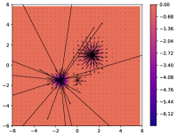
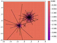
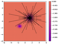
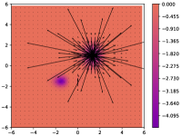
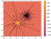
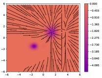
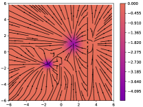
The presence of dead zones in the loss space gives rise to several problems, as listed below, which we group them together under the term “failure modes of AND-masking”.

Heavy reliance on Momentum

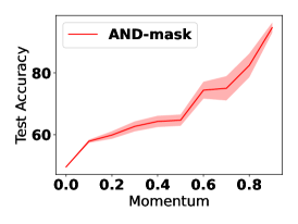
The reason that AND-masking despite the presence of dead zones in the loss landscape can practically converge to the optimal solution and capture the invariant features is that the optimizer is allowed to take advantage of the momentum of the gradients. In other words, momentum allows the optimizer to continue updating a parameter in the direction that might have been indicated several iterations ago, even if the gradients flowing in that parameter are zeroed out by AND-mask. More formally, if we model the optimizer as a function $g(.)$, the update received by component $j$ in the ILC work is

$$\begin{cases}g\left(\tilde{\nabla\mathcal{L}_{j}^{k}},M_{j}^{k}\right),&\text{if}~{}~{}\Big{|}\sum_{e}\text{sign}\big{(}[\nabla\mathcal{L}_{e}]_{j}\big{)}\Big{|}\geq\tau\\ g\left(0,M_{j}^{k}\right),&\text{otherwise}\end{cases}$$ (1)

where $\tilde{\nabla\mathcal{L}_{j}}$ is the mean of gradients from different environments, either arithmetic or geometric, and $M_{j}^{k}$ is the momentum of gradient at iteration $k$.

To verify this observation, the AND-masking is evaluated on the Spirals dataset [12] with varying values of momentum (see Fig. 2 (a)). The fact that performance is so much correlated with the momentum tells us that the deadzones are present enough in the loss landscape as to considerably impact performance when no strategy is employed to circumvent them. One could say that the high dimensionality of the model parameter space should suffice as to avoid this problem, but the failure to solve the dataset with no momentum that it doesn’t suffice as a valide escape strategy of the deadzones.

(a)

(b)

(c)

Figure 2: Test accuracy of AND-mask on the Spirals dataset [12] over 20 seeds with best known hyperparameters of AND-mask on Spirals. (a) under different values of momentum; (b) under different amplitude of noise added to the invariant dimensions of the spirals dataset; (c) under different initializations.

Sensitivity of AND-masking:

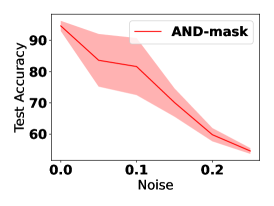
Employing a strict sign function to capture the direction of gradients followed by a heaviside function to form the AND-mask results in a sensitive process that can be deluded by infinitesimal gradients that might act as noise on the masking process. In the ILC regime, all the gradients, regardless of their magnitude, have equal contribution to the formation of the mask. This means that a small perturbation on an uncertain gradient of small magnitude can flip its sign and intrigue the AND-mask to zero out the whole set of gradients from all environment. As the results in Fig. 2 (b) suggest, the AND-masking technique is highly sensitive to noisy data and a decrease in its performance is observed over different levels of noise.

Convergence is highly dependent on initialization:

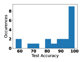
The presence of dead zones and the fact that getting stuck in a dead zone is proportional to the value of $\tau$, render a high degree of importance for the initialization of the model. Initializing a model such that some of its parameters are already in a dead zone or are likely to get stuck in one significantly restricts the possible pool of solutions to which the model has access. This creates outlier solutions that are undesirable in the OOD scenario where we don’t have access to the test set to know how our model generalizes to unseen trials. A preferable behavior would be to have less outliers to improve robustness on real-world datasets. To verify this, please refer to Fig. 2 (c), where we have experimentally validated the susceptibility of AND-masking to initialization.

3.3 The Proposed SAND-mask

In this section, we propose an enhanced version of the AND-masking technique, referred to as “SAND-mask”, which not only inherits the core idea behind the AND-masking technique, but also addresses its failure modes. In other words, as opposed to AND-mask that a strict criteria on matching the direction of gradients from all environments is applied, SAND-mask employs a smooth function capture and promote the invariant features among training domains. SAND-mask is formulated as

$$m_{\tau}=\text{max}\left(0,\text{tanh}\left(\frac{1}{\sigma^{2}}\left(\left|\frac{1}{|\mathcal{E}|}\sum_{e\in\mathcal{E}}\text{sign}(\nabla\mathcal{L}_{e})\right|-\tau\right)\right)\right),$$ (2)

where $\tau$ is the agreement threshold the determines the fraction of environments that need to agree in terms of direction of their gradients. In addition, SAND-mask introduces a new parameter, $\sigma^{2}$, to measure the dispersion of the magnitude of gradients and encourages the agreement of magnitude as well as direction among the environments. $\sigma^{2}_{j}$ for each component of network and across all environments can be calculated as

$$\sigma^{2}_{j}=\frac{\text{var}(\nabla\mathcal{L}_{j})}{\text{avg}(\nabla\mathcal{L}_{j})^{2}}.$$ (3)

Figure 3: Behavior of SAND-mask for different levels of agreement among the magnitude of gradients, when $\tau=0.9$. As it is understood, SAND-mask replicates the AND-mask only when there is a high level of agreement among the magnitude of the gradients. Otherwise, it lowers the weight assigned to the gradients to control the speed of training and avoid getting overconfident on spurious correlations in the training data.

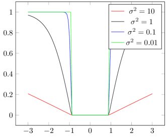
As shown in Fig. 3, SAND-mask changes its shape dynamically and based on the agreement among the magnitude of gradients such that a higher agreement is more likely to be weighted by “$1$” and vice versa. In other words, SAND-mask introduces a continuous weighting scheme to construct the mask that is in contrast with the Boolean mask created by the AND-masking technique. Since in SAND-mask the direction and the magnitude of gradients are simultaneously checked to verify the agreement among environments, one can reduce the probability of getting stuck in deadzones by lowering the agreement threshold, $\tau$. Please note that although lowering the agreement threshold might not be a reasonable strategy as we are interested in full agreement among environments but the dynamic behavior of SAND-mask that assigns a weight proportional to the degree of agreement among the magnitude of gradients would still help the model to capture the invariant features. As a final note, our proposed masking strategy significantly reduces the number of dead zones in the loss space by introducing a transient space between “full-agreement” and “no-agreement” cases (orthants) among the gradients.

We believe that although the alignment of directions among gradients is a desirable/informative measure of consistency among environments, this property can be easily counterfeited by small/noisy/outlier gradients. In such cases, the consistency of magnitude could serve as an additional clue to decide if the gradients from different environments are confidently reporting a certain direction and update to the parameter or not.

4 Experiments

In this section, the evaluation results of our proposed SAND-masking technique over well-known and popular domain generalization datasets is provided. In what follows, the benchmark on which our work is implemented and compared with other state-of-the-art techniques is introduced.

4.1 Domain Generalization Benchmark; DomainBed

DomainBed [14] provides a platform to study domain generalization of any algorithm across several benchmarking datasets and under a rigorous model selection and hyperparameter search. The core idea behind DomainBed is that the performance of domain generalization algorithms is heavily dependent on the architecture and the hyperparameters used. Therefore, DomainBed proposes three different model selection schemes based on how the validation set upon which the hyperparameters are fine tuned is formed. The three schemes are as follows:

• Training-domain Validation Set: In this scenario, the validation set is formed by randomly collecting $20\%$ of data from each of the training domains. This scenario imposes the most strict condition on hyperparameter fine tuning of the models.

• Leave-one-domain-out Cross-validation: Assuming that $n_{e}$ training domains are in hand, DomainBed trains $n_{e}$ models based on the training data from $n_{e}-1$ domains, while keeping the hyperparameters the same for all of the domains. Afterwards, the validation accuracy is reported as the average accuracy of all of the $n_{e}$ domains, which then will be the basis for fine tuning the hyperparameters.

• Test-domain validation set (Oracle) In this scenario, the validation set is formed based on the data in the test domains, and the hyper parameters are tuned based on test-time performance. However, to avoid rendering the problem as domain adaptation instead of domain generalization, access to the validation set is only feasible at the end of the training and therefore, early stopping of the training is not feasible. Please note that in this scenario, all the models based on different algorithms should undergo a fixed number of training steps to be fairly compared with each other.

In this work, we have evaluated the SAND-mask based on the first and the third validation scenarios as the Leave-one-domain-out Cross-validation is considerably expensive from computational point of view. The datasets used for our evaluations include Colored MNIST [6], Rotated MNIST [22], VLCS [23], PACS [24], Terra Incognita [25] and Office-Home [26]. The summary of our evaluations of SAND-mask and comparisons with its counterparts are provided in Tables 1 and 2, where the former summarizes the performance in “training-domain validation set”, while the latter shows the performance in “test-domain validation set”. The details of our experiments including the architectures employed and the range of hyperparameters for each model are given in Appendix A, and a comprehensive summary of the performances for all algorithms across all of the datasets is provided in Appendix B.

In addition to the above experiments, we have evaluated our work over the Spirals dataset [12], which is the original testbed for the AND-masking technique. Due to the complex nature of this dataset and its considerably higher number of domains ($16$ environments) compared to other datasets, we have only compared SAND-mask with AND-mask, IRM, and the ERM technique, as the results can be found in Table 3.

Table 1: Model selection: Training-domain Validation Set

Algorithm ColoredMNIST RotatedMNIST VLCS PACS OfficeHome TerraIncognita DomainNet Avg ERM 51.5 $\pm$ 0.1 98.0 $\pm$ 0.0 77.5 $\pm$ 0.4 85.5 $\pm$ 0.2 66.5 $\pm$ 0.3 46.1 $\pm$ 1.8 40.9 $\pm$ 0.1 66.6 IRM 52.0 $\pm$ 0.1 97.7 $\pm$ 0.1 78.5 $\pm$ 0.5 83.5 $\pm$ 0.8 64.3 $\pm$ 2.2 47.6 $\pm$ 0.8 33.9 $\pm$ 2.8 65.4 GroupDRO 52.1 $\pm$ 0.0 98.0 $\pm$ 0.0 76.7 $\pm$ 0.6 84.4 $\pm$ 0.8 66.0 $\pm$ 0.7 43.2 $\pm$ 1.1 33.3 $\pm$ 0.2 64.8 Mixup 52.1 $\pm$ 0.2 98.0 $\pm$ 0.1 77.4 $\pm$ 0.6 84.6 $\pm$ 0.6 68.1 $\pm$ 0.3 47.9 $\pm$ 0.8 39.2 $\pm$ 0.1 66.7 MLDG 51.5 $\pm$ 0.1 97.9 $\pm$ 0.0 77.2 $\pm$ 0.4 84.9 $\pm$ 1.0 66.8 $\pm$ 0.6 47.7 $\pm$ 0.9 41.2 $\pm$ 0.1 66.7 CORAL 51.5 $\pm$ 0.1 98.0 $\pm$ 0.1 78.8 $\pm$ 0.6 86.2 $\pm$ 0.3 68.7 $\pm$ 0.3 47.6 $\pm$ 1.0 41.5 $\pm$ 0.1 67.5 MMD 51.5 $\pm$ 0.2 97.9 $\pm$ 0.0 77.5 $\pm$ 0.9 84.6 $\pm$ 0.5 66.3 $\pm$ 0.1 42.2 $\pm$ 1.6 23.4 $\pm$ 9.5 63.3 DANN 51.5 $\pm$ 0.3 97.8 $\pm$ 0.1 78.6 $\pm$ 0.4 83.6 $\pm$ 0.4 65.9 $\pm$ 0.6 46.7 $\pm$ 0.5 38.3 $\pm$ 0.1 66.1 CDANN 51.7 $\pm$ 0.1 97.9 $\pm$ 0.1 77.5 $\pm$ 0.1 82.6 $\pm$ 0.9 65.8 $\pm$ 1.3 45.8 $\pm$ 1.6 38.3 $\pm$ 0.3 65.6 MTL 51.4 $\pm$ 0.1 97.9 $\pm$ 0.0 77.2 $\pm$ 0.4 84.6 $\pm$ 0.5 66.4 $\pm$ 0.5 45.6 $\pm$ 1.2 40.6 $\pm$ 0.1 66.2 SagNet 51.7 $\pm$ 0.0 98.0 $\pm$ 0.0 77.8 $\pm$ 0.5 86.3 $\pm$ 0.2 68.1 $\pm$ 0.1 48.6 $\pm$ 1.0 40.3 $\pm$ 0.1 67.2 ARM 56.2 $\pm$ 0.2 98.2 $\pm$ 0.1 77.6 $\pm$ 0.3 85.1 $\pm$ 0.4 64.8 $\pm$ 0.3 45.5 $\pm$ 0.3 35.5 $\pm$ 0.2 66.1 VREx 51.8 $\pm$ 0.1 97.9 $\pm$ 0.1 78.3 $\pm$ 0.2 84.9 $\pm$ 0.6 66.4 $\pm$ 0.6 46.4 $\pm$ 0.6 33.6 $\pm$ 2.9 65.6 RSC 51.7 $\pm$ 0.2 97.6 $\pm$ 0.1 77.1 $\pm$ 0.5 85.2 $\pm$ 0.9 65.5 $\pm$ 0.9 46.6 $\pm$ 1.0 38.9 $\pm$ 0.5 66.1 AND-mask 51.3 $\pm$ 0.2 97.6 $\pm$ 0.1 78.1 $\pm$ 0.9 84.4 $\pm$ 0.9 65.6 $\pm$ 0.4 44.6 $\pm$ 0.3 37.2$\pm$ 0.6 65.5 SAND-mask 51.8 $\pm$ 0.2 97.4 $\pm$ 0.1 77.4 $\pm$ 0.2 84.6 $\pm$ 0.9 65.8 $\pm$ 0.4 42.9 $\pm$ 1.7 32.1$\pm$ 0.6 64.6

Table 2: Model Selection: Test-domain Validation Set (Oracle)

Algorithm ColoredMNIST RotatedMNIST VLCS PACS OfficeHome TerraIncognita DomainNet Avg ERM 57.8 $\pm$ 0.2 97.8 $\pm$ 0.1 77.6 $\pm$ 0.3 86.7 $\pm$ 0.3 66.4 $\pm$ 0.5 53.0 $\pm$ 0.3 41.3 $\pm$ 0.1 68.7 IRM 67.7 $\pm$ 1.2 97.5 $\pm$ 0.2 76.9 $\pm$ 0.6 84.5 $\pm$ 1.1 63.0 $\pm$ 2.7 50.5 $\pm$ 0.7 28.0 $\pm$ 5.1 66.9 GroupDRO 61.1 $\pm$ 0.9 97.9 $\pm$ 0.1 77.4 $\pm$ 0.5 87.1 $\pm$ 0.1 66.2 $\pm$ 0.6 52.4 $\pm$ 0.1 33.4 $\pm$ 0.3 67.9 Mixup 58.4 $\pm$ 0.2 98.0 $\pm$ 0.1 78.1 $\pm$ 0.3 86.8 $\pm$ 0.3 68.0 $\pm$ 0.2 54.4 $\pm$ 0.3 39.6 $\pm$ 0.1 69.0 MLDG 58.2 $\pm$ 0.4 97.8 $\pm$ 0.1 77.5 $\pm$ 0.1 86.8 $\pm$ 0.4 66.6 $\pm$ 0.3 52.0 $\pm$ 0.1 41.6 $\pm$ 0.1 68.7 CORAL 58.6 $\pm$ 0.5 98.0 $\pm$ 0.0 77.7 $\pm$ 0.2 87.1 $\pm$ 0.5 68.4 $\pm$ 0.2 52.8 $\pm$ 0.2 41.8 $\pm$ 0.1 69.2 MMD 63.3 $\pm$ 1.3 98.0 $\pm$ 0.1 77.9 $\pm$ 0.1 87.2 $\pm$ 0.1 66.2 $\pm$ 0.3 52.0 $\pm$ 0.4 23.5 $\pm$ 9.4 66.9 DANN 57.0 $\pm$ 1.0 97.9 $\pm$ 0.1 79.7 $\pm$ 0.5 85.2 $\pm$ 0.2 65.3 $\pm$ 0.8 50.6 $\pm$ 0.4 38.3 $\pm$ 0.1 67.7 CDANN 59.5 $\pm$ 2.0 97.9 $\pm$ 0.0 79.9 $\pm$ 0.2 85.8 $\pm$ 0.8 65.3 $\pm$ 0.5 50.8 $\pm$ 0.6 38.5 $\pm$ 0.2 68.2 MTL 57.6 $\pm$ 0.3 97.9 $\pm$ 0.1 77.7 $\pm$ 0.5 86.7 $\pm$ 0.2 66.5 $\pm$ 0.4 52.2 $\pm$ 0.4 40.8 $\pm$ 0.1 68.5 SagNet 58.2 $\pm$ 0.3 97.9 $\pm$ 0.0 77.6 $\pm$ 0.1 86.4 $\pm$ 0.4 67.5 $\pm$ 0.2 52.5 $\pm$ 0.4 40.8 $\pm$ 0.2 68.7 ARM 63.2 $\pm$ 0.7 98.1 $\pm$ 0.1 77.8 $\pm$ 0.3 85.8 $\pm$ 0.2 64.8 $\pm$ 0.4 51.2 $\pm$ 0.5 36.0 $\pm$ 0.2 68.1 VREx 67.0 $\pm$ 1.3 97.9 $\pm$ 0.1 78.1 $\pm$ 0.2 87.2 $\pm$ 0.6 65.7 $\pm$ 0.3 51.4 $\pm$ 0.5 30.1 $\pm$ 3.7 68.2 RSC 58.5 $\pm$ 0.5 97.6 $\pm$ 0.1 77.8 $\pm$ 0.6 86.2 $\pm$ 0.5 66.5 $\pm$ 0.6 52.1 $\pm$ 0.2 38.9 $\pm$ 0.6 68.2 AND-mask 58.6 $\pm$ 0.4 97.5 $\pm$ 0.0 76.4 $\pm$ 0.4 86.4 $\pm$ 0.4 66.1 $\pm$ 0.2 49.8 $\pm$ 0.4 37.9$\pm$ 0.6 67.5 SAND-mask 62.3 $\pm$ 1.0 97.4 $\pm$ 0.1 76.2 $\pm$ 0.5 85.9 $\pm$ 0.4 65.9 $\pm$ 0.5 50.2 $\pm$ 0.1 32.3$\pm$ 0.6. 67.2

Table 3: Experiments on the Spiral dataset

Algorithm Training-domain Validation Set Test-domain Validation Set (Oracle) ERM 45.8 $\pm$ 2.4 94.2 $\pm$ 1.3 IRM 54.7 $\pm$ 3.6 89.0 $\pm$ 1.2 AND-mask 88.0 $\pm$ 2.9 97.25 $\pm$ 0.3 SAND-mask 49.2 $\pm$ 5.4 91.1 $\pm$ 2.4

5 Discussion

In this work, we introduced Smoothed-AND (SAND)-masking technique that improves the performance of the current state-of-the-art OOD methods over a variety of datasets. In fact, SAND-mask aims at addressing the failure modes that we identified for a recent major contributions in the field of OOD generalization, i.e., Reference [12]. As it is supported by a rigorous and exhaustive set of results on the DomainBed benchmark, SAND-mask outperforms its counterparts and significantly enhances the classification accuracy over the Colored MNIST dataset for about $6\%$. Despite the superior performance of SAND-mask over different datasets, in what follows, we elaborate on its limitations and potential direction to be pursued in future.

Limitations and Future Work:

(1) Although SAND-mask aims at replicating the behavior of AND-masking technique, the results in Table 3 show that it barely matches the performance of AND-mask over the Spiral dataset. However and on the other hand, SAND-mask manages to outperform or perform similarly to AND-mask on other OOD generalization datasets, especially on the Colored MNIST dataset that there is a performance gap of $~{}15\%$. This behavior needs to be further investigated as it seems that Spiral dataset looks at OOD generalization from a different point of view than other datasets in the field. Our SAND-mask technique has shown the capacity to bridge the two views and provide a more general solution but it needs to be studied in more depth. (2) Since the masking strategies, including AND-mask and SAND-mask, are not a penalty to the objective function, upon their satisfaction in the training phase, they are unable of stopping the training procedure as the objective function might still calculate a considerable loss over the training data. Therefore, this property leads to a self destructive behavior during training as the objective function is always trying to pull the model towards a lower loss, even though it is not optimal for generalization of the model. This limitation also requires further attention so that the objective function can get a signal of how matched the Hessians of the environments have became during the training.

Broader Impacts:

The collective efforts towards enhancing the performance of machine learning models in OOD settings is to further facilitate their widespread application in different domains, without the need to collect new domain-specific datasets and retraining the model. For instance, OOD generalization techniques can improve the performance of the deep learning models that are used in medical settings, e.g. medical imaging, as the differences in the skin tone, body shape and so many other factors related to people and diseases across the globe resemble the out of domain/distribution setting that we investigate in our experiments. In addition, the power of OOD methods in disentangling the invariant features from the ones that are spuriously correlated with the data can significantly help reducing the medical errors that happen when the training data for such models is not homogeneously collected.

Another positive impact of considering OOD methods, in general, is that facial recognition systems are prone to shift from training distribution, mainly when the source of these shifts is related to skin tone or color. So all efforts towards reducing the failure of existing OOD approaches can overcome the possible discrimination caused by facial recognition systems that are vastly used in different applications.

Appendix A Experiment

A.1 Implementation Details

Experiment where performed on the DomainBed [14] suite (MIT License) with the added Spirals dataset. All experimentation where done on an internal cluster over 1 week on 50 NVIDIA Quadro RTX 8000 GPUs.

Hyperparameter Search

For each algorithm and test environment for a given dataset we perform a random search of hyperparameters over 20 sampled configurations from distributions (see Table 4). We split the data from each domain into 80% and 20% splits. We use the 80% split for training and final evaluation of the model and use the hidden 20% split for hyperparameter selection process.

Table 4: Hyperparameters, their default values and distributions for random search for the AND-mask and SAND-mask algorithms. Hyperparameter search space of baselines can be found in the original work of Gulrajani and Lopez-Paz [14] from which results were taken from.

Condition	Parameter	Default value	Random distribution
VLCS / PACS	learning rate	0.00005	$10^{\text{Uniform}(-5,-3.5)}$
TerraIncognita	batch size	32	$2^{\text{Uniform}(3,5.5)}$
OfficeHome	weight decay	0	$10^{\text{Uniform}(-6,-2)}$
Rotated MNIST	learning rate	0.001	$10^{\text{Uniform}(-4.5,-3.5)}$
Colored MNIST	batch size	64	$2^{\text{Uniform}(3,9)}$
	weight decay	0	$0$
Spirals	learning rate	0.01	$10^{\text{Uniform}(-3.5,-1.5)}$
	batch size	512	$2^{\text{Uniform}(3,9)}$
	weight decay	$0.001$	$10^{\text{Uniform}(-6,-2)}$
	MLP depth	3	$\text{RandomChoice}([3,4,5])$
	MLP width	256	$2^{\text{Uniform}([6,10])}$
AND-mask	$\tau$	1	$\text{Uniform}(0,1)$
SAND-mask
All	dropout	0	$\text{RandomChoice}([0,0.1,0.5])$

Error bars

For each of the 20 sampled hyperparameter configuration of algorithm and test environment pairs for a given dataset, we test 3 different seeds in order to standardize the performance of a given configuration and give us estimated error bars.

Baselines

Baselines for the datasets were taken directly from the most recent set of results of the DomainBed [14] suite. Results for AND-mask and SAND-mask on all the datasets were obtained under the exact same setup which allows us to compare both set of results. Here is the list of algorithms that SAND-mask is compared with.

• ERM: Empirical Risk Minimization by Vapnik [27]

• IRM: Invariant Risk Minimization by Arjovsky et al. [6]

• GroupDRO: Group Distributionally Robust Optimization by Sagawa et al. [28]

• Mixup: Interdomain Mixup by Yan et al. [29]

• MTL: Marginal Transfer Learning by Blanchard et al. [30]

• MLDG: Meta Learning Domain Generalization by Li et al. [31]

• MMD: Maximum Mean Discrepancy by Li et al. [32]

• CORAL: Deep CORAL by Sun and Saenko [33]

• DANN: Domain Adversarial Neural Network by Ganin et al. [34]

• CDANN: Conditional Domain Adversarial Neural Network by Li et al. [35]

• SagNet: Style Agnostic Networks by Nam et al. [36]

• ARM: Adaptive Risk Minimization by Zhang et al. [37]

• VREx: Variance Risk Extrapolation by Krueger et al. [15]

• RSC: Representation Self-Challenging by Huang et al. [38]

• SD: Spectral Decoupling by Pezeshki et al. [39]

• AND-mask: Learning Explanations that are Hard to Vary by Parascandolo et al. [12]

Employed Architecture

In Table 6, we detail the architecture used for experimentation. For the MLP architecture, it’s depth and width are defined as hyperparameter included in the hyperparameter search. For the ResNet-50 architecture, we use a ResNet-50 model pretrained on ImageNet of which we replace the final layer and fine-tune. The details regarding the architecture of the MNSIT ConvNet are given in Table 6.

Table 5: Neural network architectures used for each dataset.

Dataset	Architecture
Spirals	MLP
Colored MNIST	MNIST ConvNet
Rotated MNIST
PACS	ResNet-50
VLCS
Office-Home
TerraIncognita
DomainNet

Table 6: Details of our MNIST ConvNet architecture. All convolutions use 3 $\times$ 3 kernels and “same” padding.

#	Layer
1	Conv2D (in=$d$, out=64)
2	ReLU
3	GroupNorm (groups=8)
4	Conv2D (in=64, out=128, stride=2)
5	ReLU
6	GroupNorm (8 groups)
7	Conv2D (in=128, out=128)
8	ReLU
9	GroupNorm (8 groups)
10	Conv2D (in=128, out=128)
11	ReLU
12	GroupNorm (8 groups)
13	Global average-pooling

Appendix B Supplementary Results

B.1 Spirals

Model selection method: training domain validation set Algorithm 0 1 2 3 4 5 6 7 8 9 10 11 12 13 14 15 Avg ERM 51.4 $\pm$ 0.8 55.4 $\pm$ 18.4 45.8 $\pm$ 22.0 40.9 $\pm$ 4.9 20.9 $\pm$ 11.9 59.3 $\pm$ 6.8 36.5 $\pm$ 10.1 44.8 $\pm$ 15.3 33.3 $\pm$ 27.2 17.5 $\pm$ 14.0 68.0 $\pm$ 5.0 62.7 $\pm$ 15.3 54.5 $\pm$ 5.3 27.8 $\pm$ 16.1 49.1 $\pm$ 21.9 64.6 $\pm$ 26.4 45.8 IRM 50.4 $\pm$ 0.9 37.5 $\pm$ 15.7 80.3 $\pm$ 11.5 77.7 $\pm$ 12.2 54.7 $\pm$ 23.3 64.8 $\pm$ 14.8 16.3 $\pm$ 12.2 49.6 $\pm$ 23.4 49.1 $\pm$ 20.3 45.1 $\pm$ 18.7 25.7 $\pm$ 10.4 48.3 $\pm$ 21.2 71.5 $\pm$ 12.0 58.2 $\pm$ 18.2 79.3 $\pm$ 12.3 66.1 $\pm$ 27.0 54.7 AND-mask 52.6 $\pm$ 0.5 99.7 $\pm$ 0.2 100.0 $\pm$ 0.0 99.6 $\pm$ 0.4 66.4 $\pm$ 27.1 99.9 $\pm$ 0.1 100.0 $\pm$ 0.0 100.0 $\pm$ 0.0 100.0 $\pm$ 0.0 100.0 $\pm$ 0.0 97.8 $\pm$ 1.0 99.7 $\pm$ 0.1 82.1 $\pm$ 14.6 45.4 $\pm$ 23.5 99.8 $\pm$ 0.2 66.4 $\pm$ 27.1 88.0 SAND-mask 51.9 $\pm$ 0.4 1.1 $\pm$ 0.9 33.3 $\pm$ 27.2 56.2 $\pm$ 18.3 33.3 $\pm$ 13.6 44.4 $\pm$ 22.9 74.9 $\pm$ 19.8 60.0 $\pm$ 17.8 37.2 $\pm$ 11.0 89.9 $\pm$ 8.3 69.0 $\pm$ 9.0 49.1 $\pm$ 2.1 66.6 $\pm$ 13.7 80.0 $\pm$ 16.3 25.5 $\pm$ 20.6 16.4 $\pm$ 13.4 49.2

Model selection method: test-domain validation set (oracle) Algorithm 0 1 2 3 4 5 6 7 8 9 10 11 12 13 14 15 Avg ERM 49.3 $\pm$ 0.3 98.3 $\pm$ 1.0 97.8 $\pm$ 1.8 100.0 $\pm$ 0.0 100.0 $\pm$ 0.0 91.6 $\pm$ 6.8 94.2 $\pm$ 4.7 100.0 $\pm$ 0.0 99.3 $\pm$ 0.5 96.5 $\pm$ 2.9 92.1 $\pm$ 6.4 95.8 $\pm$ 1.9 100.0 $\pm$ 0.0 99.0 $\pm$ 0.8 96.2 $\pm$ 2.3 97.4 $\pm$ 2.1 94.2 IRM 50.1 $\pm$ 0.4 100.0 $\pm$ 0.0 83.1 $\pm$ 7.8 99.3 $\pm$ 0.6 98.7 $\pm$ 1.1 90.5 $\pm$ 7.8 92.6 $\pm$ 4.2 90.5 $\pm$ 7.7 93.0 $\pm$ 1.0 86.8 $\pm$ 10.8 100.0 $\pm$ 0.0 90.8 $\pm$ 7.5 87.5 $\pm$ 10.2 75.9 $\pm$ 5.5 98.2 $\pm$ 1.5 86.3 $\pm$ 2.5 89.0 AND-mask 63.5 $\pm$ 6.0 100.0 $\pm$ 0.0 100.0 $\pm$ 0.0 95.5 $\pm$ 3.7 100.0 $\pm$ 0.0 100.0 $\pm$ 0.0 100.0 $\pm$ 0.0 100.0 $\pm$ 0.0 100.0 $\pm$ 0.0 100.0 $\pm$ 0.0 100.0 $\pm$ 0.0 100.0 $\pm$ 0.0 100.0 $\pm$ 0.0 97.0 $\pm$ 2.4 100.0 $\pm$ 0.0 100.0 $\pm$ 0.0 97.25 SAND-mask 56.2 $\pm$ 1.6 83.3 $\pm$ 13.6 100.0 $\pm$ 0.0 100.0 $\pm$ 0.0 100.0 $\pm$ 0.0 100.0 $\pm$ 0.0 96.2 $\pm$ 3.1 98.5 $\pm$ 1.3 83.0 $\pm$ 13.8 91.9 $\pm$ 6.4 100.0 $\pm$ 0.0 83.0 $\pm$ 13.9 84.9 $\pm$ 6.7 100.0 $\pm$ 0.0 85.6 $\pm$ 11.8 100.0 $\pm$ 0.0 91.1

B.2 ColoredMNIST

Model selection method: training domain validation set Algorithm +90% +80% -90% Avg ERM 71.7 $\pm$ 0.1 72.9 $\pm$ 0.2 10.0 $\pm$ 0.1 51.5 IRM 72.5 $\pm$ 0.1 73.3 $\pm$ 0.5 10.2 $\pm$ 0.3 52.0 GroupDRO 73.1 $\pm$ 0.3 73.2 $\pm$ 0.2 10.0 $\pm$ 0.2 52.1 Mixup 72.7 $\pm$ 0.4 73.4 $\pm$ 0.1 10.1 $\pm$ 0.1 52.1 MLDG 71.5 $\pm$ 0.2 73.1 $\pm$ 0.2 9.8 $\pm$ 0.1 51.5 CORAL 71.6 $\pm$ 0.3 73.1 $\pm$ 0.1 9.9 $\pm$ 0.1 51.5 MMD 71.4 $\pm$ 0.3 73.1 $\pm$ 0.2 9.9 $\pm$ 0.3 51.5 DANN 71.4 $\pm$ 0.9 73.1 $\pm$ 0.1 10.0 $\pm$ 0.0 51.5 CDANN 72.0 $\pm$ 0.2 73.0 $\pm$ 0.2 10.2 $\pm$ 0.1 51.7 MTL 70.9 $\pm$ 0.2 72.8 $\pm$ 0.3 10.5 $\pm$ 0.1 51.4 SagNet 71.8 $\pm$ 0.2 73.0 $\pm$ 0.2 10.3 $\pm$ 0.0 51.7 ARM 82.0 $\pm$ 0.5 76.5 $\pm$ 0.3 10.2 $\pm$ 0.0 56.2 VREx 72.4 $\pm$ 0.3 72.9 $\pm$ 0.4 10.2 $\pm$ 0.0 51.8 RSC 71.9 $\pm$ 0.3 73.1 $\pm$ 0.2 10.0 $\pm$ 0.2 51.7 AND-mask 70.7 $\pm$ 0.5 73.3 $\pm$ 0.2 10.0 $\pm$ 0.1 51.3 SAND-mask 72.0 $\pm$ 0.5 73.2 $\pm$ 0.4 10.3 $\pm$ 0.2 51.8

Model selection method: test-domain validation set (oracle) Algorithm +90% +80% -90% Avg ERM 71.8 $\pm$ 0.4 72.9 $\pm$ 0.1 28.7 $\pm$ 0.5 57.8 IRM 72.0 $\pm$ 0.1 72.5 $\pm$ 0.3 58.5 $\pm$ 3.3 67.7 GroupDRO 73.5 $\pm$ 0.3 73.0 $\pm$ 0.3 36.8 $\pm$ 2.8 61.1 Mixup 72.5 $\pm$ 0.2 73.9 $\pm$ 0.4 28.6 $\pm$ 0.2 58.4 MLDG 71.9 $\pm$ 0.3 73.5 $\pm$ 0.2 29.1 $\pm$ 0.9 58.2 CORAL 71.1 $\pm$ 0.2 73.4 $\pm$ 0.2 31.1 $\pm$ 1.6 58.6 MMD 69.0 $\pm$ 2.3 70.4 $\pm$ 1.6 50.6 $\pm$ 0.2 63.3 DANN 72.4 $\pm$ 0.5 73.9 $\pm$ 0.5 24.9 $\pm$ 2.7 57.0 CDANN 71.8 $\pm$ 0.5 72.9 $\pm$ 0.1 33.8 $\pm$ 6.4 59.5 MTL 71.2 $\pm$ 0.2 73.5 $\pm$ 0.2 28.0 $\pm$ 0.6 57.6 SagNet 72.1 $\pm$ 0.3 73.2 $\pm$ 0.3 29.4 $\pm$ 0.5 58.2 ARM 84.9 $\pm$ 0.9 76.8 $\pm$ 0.6 27.9 $\pm$ 2.1 63.2 VREx 72.8 $\pm$ 0.3 73.0 $\pm$ 0.3 55.2 $\pm$ 4.0 67.0 RSC 72.0 $\pm$ 0.1 73.2 $\pm$ 0.1 30.2 $\pm$ 1.6 58.5 AND-mask 71.9 $\pm$ 0.6 73.6 $\pm$ 0.5 30.2 $\pm$ 1.4 58.6 SAND-mask 79.9 $\pm$ 3.8 75.9 $\pm$ 1.6 31.6 $\pm$ 1.1 62.3

B.3 RotatedMNIST

Model selection method: training domain validation set Algorithm 0 15 30 45 60 75 Avg ERM 95.9 $\pm$ 0.1 98.9 $\pm$ 0.0 98.8 $\pm$ 0.0 98.9 $\pm$ 0.0 98.9 $\pm$ 0.0 96.4 $\pm$ 0.0 98.0 IRM 95.5 $\pm$ 0.1 98.8 $\pm$ 0.2 98.7 $\pm$ 0.1 98.6 $\pm$ 0.1 98.7 $\pm$ 0.0 95.9 $\pm$ 0.2 97.7 GroupDRO 95.6 $\pm$ 0.1 98.9 $\pm$ 0.1 98.9 $\pm$ 0.1 99.0 $\pm$ 0.0 98.9 $\pm$ 0.0 96.5 $\pm$ 0.2 98.0 Mixup 95.8 $\pm$ 0.3 98.9 $\pm$ 0.0 98.9 $\pm$ 0.0 98.9 $\pm$ 0.0 98.8 $\pm$ 0.1 96.5 $\pm$ 0.3 98.0 MLDG 95.8 $\pm$ 0.1 98.9 $\pm$ 0.1 99.0 $\pm$ 0.0 98.9 $\pm$ 0.1 99.0 $\pm$ 0.0 95.8 $\pm$ 0.3 97.9 CORAL 95.8 $\pm$ 0.3 98.8 $\pm$ 0.0 98.9 $\pm$ 0.0 99.0 $\pm$ 0.0 98.9 $\pm$ 0.1 96.4 $\pm$ 0.2 98.0 MMD 95.6 $\pm$ 0.1 98.9 $\pm$ 0.1 99.0 $\pm$ 0.0 99.0 $\pm$ 0.0 98.9 $\pm$ 0.0 96.0 $\pm$ 0.2 97.9 DANN 95.0 $\pm$ 0.5 98.9 $\pm$ 0.1 99.0 $\pm$ 0.0 99.0 $\pm$ 0.1 98.9 $\pm$ 0.0 96.3 $\pm$ 0.2 97.8 CDANN 95.7 $\pm$ 0.2 98.8 $\pm$ 0.0 98.9 $\pm$ 0.1 98.9 $\pm$ 0.1 98.9 $\pm$ 0.1 96.1 $\pm$ 0.3 97.9 MTL 95.6 $\pm$ 0.1 99.0 $\pm$ 0.1 99.0 $\pm$ 0.0 98.9 $\pm$ 0.1 99.0 $\pm$ 0.1 95.8 $\pm$ 0.2 97.9 SagNet 95.9 $\pm$ 0.3 98.9 $\pm$ 0.1 99.0 $\pm$ 0.1 99.1 $\pm$ 0.0 99.0 $\pm$ 0.1 96.3 $\pm$ 0.1 98.0 ARM 96.7 $\pm$ 0.2 99.1 $\pm$ 0.0 99.0 $\pm$ 0.0 99.0 $\pm$ 0.1 99.1 $\pm$ 0.1 96.5 $\pm$ 0.4 98.2 VREx 95.9 $\pm$ 0.2 99.0 $\pm$ 0.1 98.9 $\pm$ 0.1 98.9 $\pm$ 0.1 98.7 $\pm$ 0.1 96.2 $\pm$ 0.2 97.9 RSC 94.8 $\pm$ 0.5 98.7 $\pm$ 0.1 98.8 $\pm$ 0.1 98.8 $\pm$ 0.0 98.9 $\pm$ 0.1 95.9 $\pm$ 0.2 97.6 AND-mask 94.8 $\pm$ 0.2 98.8 $\pm$ 0.1 98.9 $\pm$ 0.0 98.7 $\pm$ 0.0 98.7 $\pm$ 0.1 95.5 $\pm$ 0.4 97.6 SAND-mask 94.5 $\pm$ 0.4 98.6 $\pm$ 0.1 98.8 $\pm$ 0.1 98.7 $\pm$ 0.1 98.6 $\pm$ 0.0 95.5 $\pm$ 0.2 97.4

Model selection method: test-domain validation set (oracle) Algorithm 0 15 30 45 60 75 Avg ERM 95.3 $\pm$ 0.2 98.7 $\pm$ 0.1 98.9 $\pm$ 0.1 98.7 $\pm$ 0.2 98.9 $\pm$ 0.0 96.2 $\pm$ 0.2 97.8 IRM 94.9 $\pm$ 0.6 98.7 $\pm$ 0.2 98.6 $\pm$ 0.1 98.6 $\pm$ 0.2 98.7 $\pm$ 0.1 95.2 $\pm$ 0.3 97.5 GroupDRO 95.9 $\pm$ 0.1 99.0 $\pm$ 0.1 98.9 $\pm$ 0.1 98.8 $\pm$ 0.1 98.6 $\pm$ 0.1 96.3 $\pm$ 0.4 97.9 Mixup 95.8 $\pm$ 0.3 98.7 $\pm$ 0.0 99.0 $\pm$ 0.1 98.8 $\pm$ 0.1 98.8 $\pm$ 0.1 96.6 $\pm$ 0.2 98.0 MLDG 95.7 $\pm$ 0.2 98.9 $\pm$ 0.1 98.8 $\pm$ 0.1 98.9 $\pm$ 0.1 98.6 $\pm$ 0.1 95.8 $\pm$ 0.4 97.8 CORAL 96.2 $\pm$ 0.2 98.8 $\pm$ 0.1 98.8 $\pm$ 0.1 98.8 $\pm$ 0.1 98.9 $\pm$ 0.1 96.4 $\pm$ 0.2 98.0 MMD 96.1 $\pm$ 0.2 98.9 $\pm$ 0.0 99.0 $\pm$ 0.0 98.8 $\pm$ 0.0 98.9 $\pm$ 0.0 96.4 $\pm$ 0.2 98.0 DANN 95.9 $\pm$ 0.1 98.9 $\pm$ 0.1 98.6 $\pm$ 0.2 98.7 $\pm$ 0.1 98.9 $\pm$ 0.0 96.3 $\pm$ 0.3 97.9 CDANN 95.9 $\pm$ 0.2 98.8 $\pm$ 0.0 98.7 $\pm$ 0.1 98.9 $\pm$ 0.1 98.8 $\pm$ 0.1 96.1 $\pm$ 0.3 97.9 MTL 96.1 $\pm$ 0.2 98.9 $\pm$ 0.0 99.0 $\pm$ 0.0 98.7 $\pm$ 0.1 99.0 $\pm$ 0.0 95.8 $\pm$ 0.3 97.9 SagNet 95.9 $\pm$ 0.1 99.0 $\pm$ 0.1 98.9 $\pm$ 0.1 98.6 $\pm$ 0.1 98.8 $\pm$ 0.1 96.3 $\pm$ 0.1 97.9 ARM 95.9 $\pm$ 0.4 99.0 $\pm$ 0.1 98.8 $\pm$ 0.1 98.9 $\pm$ 0.1 99.1 $\pm$ 0.1 96.7 $\pm$ 0.2 98.1 VREx 95.5 $\pm$ 0.2 99.0 $\pm$ 0.0 98.7 $\pm$ 0.2 98.8 $\pm$ 0.1 98.8 $\pm$ 0.0 96.4 $\pm$ 0.0 97.9 RSC 95.4 $\pm$ 0.1 98.6 $\pm$ 0.1 98.6 $\pm$ 0.1 98.9 $\pm$ 0.0 98.8 $\pm$ 0.1 95.4 $\pm$ 0.3 97.6 AND-mask 94.9 $\pm$ 0.1 98.8 $\pm$ 0.1 98.8 $\pm$ 0.1 98.7 $\pm$ 0.2 98.6 $\pm$ 0.2 95.5 $\pm$ 0.2 97.5 SAND-mask 94.7 $\pm$ 0.2 98.5 $\pm$ 0.2 98.6 $\pm$ 0.1 98.6 $\pm$ 0.1 98.5 $\pm$ 0.1 95.2 $\pm$ 0.1 97.4

B.4 VLCS

Model selection method: training domain validation set Algorithm C L S V Avg ERM 97.7 $\pm$ 0.4 64.3 $\pm$ 0.9 73.4 $\pm$ 0.5 74.6 $\pm$ 1.3 77.5 IRM 98.6 $\pm$ 0.1 64.9 $\pm$ 0.9 73.4 $\pm$ 0.6 77.3 $\pm$ 0.9 78.5 GroupDRO 97.3 $\pm$ 0.3 63.4 $\pm$ 0.9 69.5 $\pm$ 0.8 76.7 $\pm$ 0.7 76.7 Mixup 98.3 $\pm$ 0.6 64.8 $\pm$ 1.0 72.1 $\pm$ 0.5 74.3 $\pm$ 0.8 77.4 MLDG 97.4 $\pm$ 0.2 65.2 $\pm$ 0.7 71.0 $\pm$ 1.4 75.3 $\pm$ 1.0 77.2 CORAL 98.3 $\pm$ 0.1 66.1 $\pm$ 1.2 73.4 $\pm$ 0.3 77.5 $\pm$ 1.2 78.8 MMD 97.7 $\pm$ 0.1 64.0 $\pm$ 1.1 72.8 $\pm$ 0.2 75.3 $\pm$ 3.3 77.5 DANN 99.0 $\pm$ 0.3 65.1 $\pm$ 1.4 73.1 $\pm$ 0.3 77.2 $\pm$ 0.6 78.6 CDANN 97.1 $\pm$ 0.3 65.1 $\pm$ 1.2 70.7 $\pm$ 0.8 77.1 $\pm$ 1.5 77.5 MTL 97.8 $\pm$ 0.4 64.3 $\pm$ 0.3 71.5 $\pm$ 0.7 75.3 $\pm$ 1.7 77.2 SagNet 97.9 $\pm$ 0.4 64.5 $\pm$ 0.5 71.4 $\pm$ 1.3 77.5 $\pm$ 0.5 77.8 ARM 98.7 $\pm$ 0.2 63.6 $\pm$ 0.7 71.3 $\pm$ 1.2 76.7 $\pm$ 0.6 77.6 VREx 98.4 $\pm$ 0.3 64.4 $\pm$ 1.4 74.1 $\pm$ 0.4 76.2 $\pm$ 1.3 78.3 RSC 97.9 $\pm$ 0.1 62.5 $\pm$ 0.7 72.3 $\pm$ 1.2 75.6 $\pm$ 0.8 77.1 AND-mask 97.8 $\pm$ 0.4 64.3 $\pm$ 1.2 73.5 $\pm$ 0.7 76.8 $\pm$ 2.6 78.1 SAND-mask 98.5 $\pm$ 0.3 63.6 $\pm$ 0.9 70.4 $\pm$ 0.8 77.1 $\pm$ 0.8 77.4

Model selection method: test-domain validation set (oracle) Algorithm C L S V Avg ERM 97.6 $\pm$ 0.3 67.9 $\pm$ 0.7 70.9 $\pm$ 0.2 74.0 $\pm$ 0.6 77.6 IRM 97.3 $\pm$ 0.2 66.7 $\pm$ 0.1 71.0 $\pm$ 2.3 72.8 $\pm$ 0.4 76.9 GroupDRO 97.7 $\pm$ 0.2 65.9 $\pm$ 0.2 72.8 $\pm$ 0.8 73.4 $\pm$ 1.3 77.4 Mixup 97.8 $\pm$ 0.4 67.2 $\pm$ 0.4 71.5 $\pm$ 0.2 75.7 $\pm$ 0.6 78.1 MLDG 97.1 $\pm$ 0.5 66.6 $\pm$ 0.5 71.5 $\pm$ 0.1 75.0 $\pm$ 0.9 77.5 CORAL 97.3 $\pm$ 0.2 67.5 $\pm$ 0.6 71.6 $\pm$ 0.6 74.5 $\pm$ 0.0 77.7 MMD 98.8 $\pm$ 0.0 66.4 $\pm$ 0.4 70.8 $\pm$ 0.5 75.6 $\pm$ 0.4 77.9 DANN 99.0 $\pm$ 0.2 66.3 $\pm$ 1.2 73.4 $\pm$ 1.4 80.1 $\pm$ 0.5 79.7 CDANN 98.2 $\pm$ 0.1 68.8 $\pm$ 0.5 74.3 $\pm$ 0.6 78.1 $\pm$ 0.5 79.9 MTL 97.9 $\pm$ 0.7 66.1 $\pm$ 0.7 72.0 $\pm$ 0.4 74.9 $\pm$ 1.1 77.7 SagNet 97.4 $\pm$ 0.3 66.4 $\pm$ 0.4 71.6 $\pm$ 0.1 75.0 $\pm$ 0.8 77.6 ARM 97.6 $\pm$ 0.6 66.5 $\pm$ 0.3 72.7 $\pm$ 0.6 74.4 $\pm$ 0.7 77.8 VREx 98.4 $\pm$ 0.2 66.4 $\pm$ 0.7 72.8 $\pm$ 0.1 75.0 $\pm$ 1.4 78.1 RSC 98.0 $\pm$ 0.4 67.2 $\pm$ 0.3 70.3 $\pm$ 1.3 75.6 $\pm$ 0.4 77.8 AND-mask 98.3 $\pm$ 0.3 64.5 $\pm$ 0.2 69.3 $\pm$ 1.3 73.4 $\pm$ 1.3 76.4 SAND-mask 97.6 $\pm$ 0.3 64.5 $\pm$ 0.6 69.7 $\pm$ 0.6 73.0 $\pm$ 1.2 76.2

B.5 PACS

Model selection method: training domain validation set Algorithm A C P S Avg ERM 84.7 $\pm$ 0.4 80.8 $\pm$ 0.6 97.2 $\pm$ 0.3 79.3 $\pm$ 1.0 85.5 IRM 84.8 $\pm$ 1.3 76.4 $\pm$ 1.1 96.7 $\pm$ 0.6 76.1 $\pm$ 1.0 83.5 GroupDRO 83.5 $\pm$ 0.9 79.1 $\pm$ 0.6 96.7 $\pm$ 0.3 78.3 $\pm$ 2.0 84.4 Mixup 86.1 $\pm$ 0.5 78.9 $\pm$ 0.8 97.6 $\pm$ 0.1 75.8 $\pm$ 1.8 84.6 MLDG 85.5 $\pm$ 1.4 80.1 $\pm$ 1.7 97.4 $\pm$ 0.3 76.6 $\pm$ 1.1 84.9 CORAL 88.3 $\pm$ 0.2 80.0 $\pm$ 0.5 97.5 $\pm$ 0.3 78.8 $\pm$ 1.3 86.2 MMD 86.1 $\pm$ 1.4 79.4 $\pm$ 0.9 96.6 $\pm$ 0.2 76.5 $\pm$ 0.5 84.6 DANN 86.4 $\pm$ 0.8 77.4 $\pm$ 0.8 97.3 $\pm$ 0.4 73.5 $\pm$ 2.3 83.6 CDANN 84.6 $\pm$ 1.8 75.5 $\pm$ 0.9 96.8 $\pm$ 0.3 73.5 $\pm$ 0.6 82.6 MTL 87.5 $\pm$ 0.8 77.1 $\pm$ 0.5 96.4 $\pm$ 0.8 77.3 $\pm$ 1.8 84.6 SagNet 87.4 $\pm$ 1.0 80.7 $\pm$ 0.6 97.1 $\pm$ 0.1 80.0 $\pm$ 0.4 86.3 ARM 86.8 $\pm$ 0.6 76.8 $\pm$ 0.5 97.4 $\pm$ 0.3 79.3 $\pm$ 1.2 85.1 VREx 86.0 $\pm$ 1.6 79.1 $\pm$ 0.6 96.9 $\pm$ 0.5 77.7 $\pm$ 1.7 84.9 RSC 85.4 $\pm$ 0.8 79.7 $\pm$ 1.8 97.6 $\pm$ 0.3 78.2 $\pm$ 1.2 85.2 AND-mask 85.3 $\pm$ 1.4 79.2 $\pm$ 2.0 96.9 $\pm$ 0.4 76.2 $\pm$ 1.4 84.4 SAND-mask 85.8 $\pm$ 1.7 79.2 $\pm$ 0.8 96.3 $\pm$ 0.2 76.9 $\pm$ 2.0 84.6

Model selection method: test-domain validation set (oracle) Algorithm A C P S Avg ERM 86.5 $\pm$ 1.0 81.3 $\pm$ 0.6 96.2 $\pm$ 0.3 82.7 $\pm$ 1.1 86.7 IRM 84.2 $\pm$ 0.9 79.7 $\pm$ 1.5 95.9 $\pm$ 0.4 78.3 $\pm$ 2.1 84.5 GroupDRO 87.5 $\pm$ 0.5 82.9 $\pm$ 0.6 97.1 $\pm$ 0.3 81.1 $\pm$ 1.2 87.1 Mixup 87.5 $\pm$ 0.4 81.6 $\pm$ 0.7 97.4 $\pm$ 0.2 80.8 $\pm$ 0.9 86.8 MLDG 87.0 $\pm$ 1.2 82.5 $\pm$ 0.9 96.7 $\pm$ 0.3 81.2 $\pm$ 0.6 86.8 CORAL 86.6 $\pm$ 0.8 81.8 $\pm$ 0.9 97.1 $\pm$ 0.5 82.7 $\pm$ 0.6 87.1 MMD 88.1 $\pm$ 0.8 82.6 $\pm$ 0.7 97.1 $\pm$ 0.5 81.2 $\pm$ 1.2 87.2 DANN 87.0 $\pm$ 0.4 80.3 $\pm$ 0.6 96.8 $\pm$ 0.3 76.9 $\pm$ 1.1 85.2 CDANN 87.7 $\pm$ 0.6 80.7 $\pm$ 1.2 97.3 $\pm$ 0.4 77.6 $\pm$ 1.5 85.8 MTL 87.0 $\pm$ 0.2 82.7 $\pm$ 0.8 96.5 $\pm$ 0.7 80.5 $\pm$ 0.8 86.7 SagNet 87.4 $\pm$ 0.5 81.2 $\pm$ 1.2 96.3 $\pm$ 0.8 80.7 $\pm$ 1.1 86.4 ARM 85.0 $\pm$ 1.2 81.4 $\pm$ 0.2 95.9 $\pm$ 0.3 80.9 $\pm$ 0.5 85.8 VREx 87.8 $\pm$ 1.2 81.8 $\pm$ 0.7 97.4 $\pm$ 0.2 82.1 $\pm$ 0.7 87.2 RSC 86.0 $\pm$ 0.7 81.8 $\pm$ 0.9 96.8 $\pm$ 0.7 80.4 $\pm$ 0.5 86.2 AND-mask 86.4 $\pm$ 1.1 80.8 $\pm$ 0.9 97.1 $\pm$ 0.2 81.3 $\pm$ 1.1 86.4 SAND-mask 86.1 $\pm$ 0.6 80.3 $\pm$ 1.0 97.1 $\pm$ 0.3 80.0 $\pm$ 1.3 85.9

B.6 OfficeHome

Model selection method: training domain validation set Algorithm A C P R Avg ERM 61.3 $\pm$ 0.7 52.4 $\pm$ 0.3 75.8 $\pm$ 0.1 76.6 $\pm$ 0.3 66.5 IRM 58.9 $\pm$ 2.3 52.2 $\pm$ 1.6 72.1 $\pm$ 2.9 74.0 $\pm$ 2.5 64.3 GroupDRO 60.4 $\pm$ 0.7 52.7 $\pm$ 1.0 75.0 $\pm$ 0.7 76.0 $\pm$ 0.7 66.0 Mixup 62.4 $\pm$ 0.8 54.8 $\pm$ 0.6 76.9 $\pm$ 0.3 78.3 $\pm$ 0.2 68.1 MLDG 61.5 $\pm$ 0.9 53.2 $\pm$ 0.6 75.0 $\pm$ 1.2 77.5 $\pm$ 0.4 66.8 CORAL 65.3 $\pm$ 0.4 54.4 $\pm$ 0.5 76.5 $\pm$ 0.1 78.4 $\pm$ 0.5 68.7 MMD 60.4 $\pm$ 0.2 53.3 $\pm$ 0.3 74.3 $\pm$ 0.1 77.4 $\pm$ 0.6 66.3 DANN 59.9 $\pm$ 1.3 53.0 $\pm$ 0.3 73.6 $\pm$ 0.7 76.9 $\pm$ 0.5 65.9 CDANN 61.5 $\pm$ 1.4 50.4 $\pm$ 2.4 74.4 $\pm$ 0.9 76.6 $\pm$ 0.8 65.8 MTL 61.5 $\pm$ 0.7 52.4 $\pm$ 0.6 74.9 $\pm$ 0.4 76.8 $\pm$ 0.4 66.4 SagNet 63.4 $\pm$ 0.2 54.8 $\pm$ 0.4 75.8 $\pm$ 0.4 78.3 $\pm$ 0.3 68.1 ARM 58.9 $\pm$ 0.8 51.0 $\pm$ 0.5 74.1 $\pm$ 0.1 75.2 $\pm$ 0.3 64.8 VREx 60.7 $\pm$ 0.9 53.0 $\pm$ 0.9 75.3 $\pm$ 0.1 76.6 $\pm$ 0.5 66.4 RSC 60.7 $\pm$ 1.4 51.4 $\pm$ 0.3 74.8 $\pm$ 1.1 75.1 $\pm$ 1.3 65.5 ANDMask 59.5 $\pm$ 1.2 51.7 $\pm$ 0.2 73.9 $\pm$ 0.4 77.1 $\pm$ 0.2 65.6 SAND-mask 60.3 $\pm$ 0.5 53.3 $\pm$ 0.7 73.5 $\pm$ 0.7 76.2 $\pm$ 0.3 65.8

Model selection method: test-domain validation set (oracle) Algorithm A C P R Avg ERM 61.7 $\pm$ 0.7 53.4 $\pm$ 0.3 74.1 $\pm$ 0.4 76.2 $\pm$ 0.6 66.4 IRM 56.4 $\pm$ 3.2 51.2 $\pm$ 2.3 71.7 $\pm$ 2.7 72.7 $\pm$ 2.7 63.0 GroupDRO 60.5 $\pm$ 1.6 53.1 $\pm$ 0.3 75.5 $\pm$ 0.3 75.9 $\pm$ 0.7 66.2 Mixup 63.5 $\pm$ 0.2 54.6 $\pm$ 0.4 76.0 $\pm$ 0.3 78.0 $\pm$ 0.7 68.0 MLDG 60.5 $\pm$ 0.7 54.2 $\pm$ 0.5 75.0 $\pm$ 0.2 76.7 $\pm$ 0.5 66.6 CORAL 64.8 $\pm$ 0.8 54.1 $\pm$ 0.9 76.5 $\pm$ 0.4 78.2 $\pm$ 0.4 68.4 MMD 60.4 $\pm$ 1.0 53.4 $\pm$ 0.5 74.9 $\pm$ 0.1 76.1 $\pm$ 0.7 66.2 DANN 60.6 $\pm$ 1.4 51.8 $\pm$ 0.7 73.4 $\pm$ 0.5 75.5 $\pm$ 0.9 65.3 CDANN 57.9 $\pm$ 0.2 52.1 $\pm$ 1.2 74.9 $\pm$ 0.7 76.2 $\pm$ 0.2 65.3 MTL 60.7 $\pm$ 0.8 53.5 $\pm$ 1.3 75.2 $\pm$ 0.6 76.6 $\pm$ 0.6 66.5 SagNet 62.7 $\pm$ 0.5 53.6 $\pm$ 0.5 76.0 $\pm$ 0.3 77.8 $\pm$ 0.1 67.5 ARM 58.8 $\pm$ 0.5 51.8 $\pm$ 0.7 74.0 $\pm$ 0.1 74.4 $\pm$ 0.2 64.8 VREx 59.6 $\pm$ 1.0 53.3 $\pm$ 0.3 73.2 $\pm$ 0.5 76.6 $\pm$ 0.4 65.7 RSC 61.7 $\pm$ 0.8 53.0 $\pm$ 0.9 74.8 $\pm$ 0.8 76.3 $\pm$ 0.5 66.5 ANDMask 60.3 $\pm$ 0.5 52.3 $\pm$ 0.6 75.1 $\pm$ 0.2 76.6 $\pm$ 0.3 66.1 SAND-mask 59.9 $\pm$ 0.7 53.6 $\pm$ 0.8 74.3 $\pm$ 0.4 75.8 $\pm$ 0.5 65.9

B.7 TerraIncognita

Model selection method: training domain validation set Algorithm L100 L38 L43 L46 Avg ERM 49.8 $\pm$ 4.4 42.1 $\pm$ 1.4 56.9 $\pm$ 1.8 35.7 $\pm$ 3.9 46.1 IRM 54.6 $\pm$ 1.3 39.8 $\pm$ 1.9 56.2 $\pm$ 1.8 39.6 $\pm$ 0.8 47.6 GroupDRO 41.2 $\pm$ 0.7 38.6 $\pm$ 2.1 56.7 $\pm$ 0.9 36.4 $\pm$ 2.1 43.2 Mixup 59.6 $\pm$ 2.0 42.2 $\pm$ 1.4 55.9 $\pm$ 0.8 33.9 $\pm$ 1.4 47.9 MLDG 54.2 $\pm$ 3.0 44.3 $\pm$ 1.1 55.6 $\pm$ 0.3 36.9 $\pm$ 2.2 47.7 CORAL 51.6 $\pm$ 2.4 42.2 $\pm$ 1.0 57.0 $\pm$ 1.0 39.8 $\pm$ 2.9 47.6 MMD 41.9 $\pm$ 3.0 34.8 $\pm$ 1.0 57.0 $\pm$ 1.9 35.2 $\pm$ 1.8 42.2 DANN 51.1 $\pm$ 3.5 40.6 $\pm$ 0.6 57.4 $\pm$ 0.5 37.7 $\pm$ 1.8 46.7 CDANN 47.0 $\pm$ 1.9 41.3 $\pm$ 4.8 54.9 $\pm$ 1.7 39.8 $\pm$ 2.3 45.8 MTL 49.3 $\pm$ 1.2 39.6 $\pm$ 6.3 55.6 $\pm$ 1.1 37.8 $\pm$ 0.8 45.6 SagNet 53.0 $\pm$ 2.9 43.0 $\pm$ 2.5 57.9 $\pm$ 0.6 40.4 $\pm$ 1.3 48.6 ARM 49.3 $\pm$ 0.7 38.3 $\pm$ 2.4 55.8 $\pm$ 0.8 38.7 $\pm$ 1.3 45.5 VREx 48.2 $\pm$ 4.3 41.7 $\pm$ 1.3 56.8 $\pm$ 0.8 38.7 $\pm$ 3.1 46.4 RSC 50.2 $\pm$ 2.2 39.2 $\pm$ 1.4 56.3 $\pm$ 1.4 40.8 $\pm$ 0.6 46.6 AND-mask 50.0 $\pm$ 2.9 40.2 $\pm$ 0.8 53.3 $\pm$ 0.7 34.8 $\pm$ 1.9 44.6 SAND-mask 45.7 $\pm$ 2.9 31.6 $\pm$ 4.7 55.1 $\pm$ 1.0 39.0 $\pm$ 1.8 42.9

Model selection method: test-domain validation set (oracle) Algorithm L100 L38 L43 L46 Avg ERM 59.4 $\pm$ 0.9 49.3 $\pm$ 0.6 60.1 $\pm$ 1.1 43.2 $\pm$ 0.5 53.0 IRM 56.5 $\pm$ 2.5 49.8 $\pm$ 1.5 57.1 $\pm$ 2.2 38.6 $\pm$ 1.0 50.5 GroupDRO 60.4 $\pm$ 1.5 48.3 $\pm$ 0.4 58.6 $\pm$ 0.8 42.2 $\pm$ 0.8 52.4 Mixup 67.6 $\pm$ 1.8 51.0 $\pm$ 1.3 59.0 $\pm$ 0.0 40.0 $\pm$ 1.1 54.4 MLDG 59.2 $\pm$ 0.1 49.0 $\pm$ 0.9 58.4 $\pm$ 0.9 41.4 $\pm$ 1.0 52.0 CORAL 60.4 $\pm$ 0.9 47.2 $\pm$ 0.5 59.3 $\pm$ 0.4 44.4 $\pm$ 0.4 52.8 MMD 60.6 $\pm$ 1.1 45.9 $\pm$ 0.3 57.8 $\pm$ 0.5 43.8 $\pm$ 1.2 52.0 DANN 55.2 $\pm$ 1.9 47.0 $\pm$ 0.7 57.2 $\pm$ 0.9 42.9 $\pm$ 0.9 50.6 CDANN 56.3 $\pm$ 2.0 47.1 $\pm$ 0.9 57.2 $\pm$ 1.1 42.4 $\pm$ 0.8 50.8 MTL 58.4 $\pm$ 2.1 48.4 $\pm$ 0.8 58.9 $\pm$ 0.6 43.0 $\pm$ 1.3 52.2 SagNet 56.4 $\pm$ 1.9 50.5 $\pm$ 2.3 59.1 $\pm$ 0.5 44.1 $\pm$ 0.6 52.5 ARM 60.1 $\pm$ 1.5 48.3 $\pm$ 1.6 55.3 $\pm$ 0.6 40.9 $\pm$ 1.1 51.2 VREx 56.8 $\pm$ 1.7 46.5 $\pm$ 0.5 58.4 $\pm$ 0.3 43.8 $\pm$ 0.3 51.4 RSC 59.9 $\pm$ 1.4 46.7 $\pm$ 0.4 57.8 $\pm$ 0.5 44.3 $\pm$ 0.6 52.1 AND-mask 54.7 $\pm$ 1.8 48.4 $\pm$ 0.5 55.1 $\pm$ 0.5 41.3 $\pm$ 0.6 49.8 SAND-mask 56.2 $\pm$ 1.8 46.3 $\pm$ 0.3 55.8 $\pm$ 0.4 42.6 $\pm$ 1.2 50.2

B.7.1 DomainNet

Model selection method: training domain validation set Algorithm clip info paint quick real sketch Avg ERM 58.1 $\pm$ 0.3 18.8 $\pm$ 0.3 46.7 $\pm$ 0.3 12.2 $\pm$ 0.4 59.6 $\pm$ 0.1 49.8 $\pm$ 0.4 40.9 IRM 48.5 $\pm$ 2.8 15.0 $\pm$ 1.5 38.3 $\pm$ 4.3 10.9 $\pm$ 0.5 48.2 $\pm$ 5.2 42.3 $\pm$ 3.1 33.9 GroupDRO 47.2 $\pm$ 0.5 17.5 $\pm$ 0.4 33.8 $\pm$ 0.5 9.3 $\pm$ 0.3 51.6 $\pm$ 0.4 40.1 $\pm$ 0.6 33.3 Mixup 55.7 $\pm$ 0.3 18.5 $\pm$ 0.5 44.3 $\pm$ 0.5 12.5 $\pm$ 0.4 55.8 $\pm$ 0.3 48.2 $\pm$ 0.5 39.2 MLDG 59.1 $\pm$ 0.2 19.1 $\pm$ 0.3 45.8 $\pm$ 0.7 13.4 $\pm$ 0.3 59.6 $\pm$ 0.2 50.2 $\pm$ 0.4 41.2 CORAL 59.2 $\pm$ 0.1 19.7 $\pm$ 0.2 46.6 $\pm$ 0.3 13.4 $\pm$ 0.4 59.8 $\pm$ 0.2 50.1 $\pm$ 0.6 41.5 MMD 32.1 $\pm$ 13.3 11.0 $\pm$ 4.6 26.8 $\pm$ 11.3 8.7 $\pm$ 2.1 32.7 $\pm$ 13.8 28.9 $\pm$ 11.9 23.4 DANN 53.1 $\pm$ 0.2 18.3 $\pm$ 0.1 44.2 $\pm$ 0.7 11.8 $\pm$ 0.1 55.5 $\pm$ 0.4 46.8 $\pm$ 0.6 38.3 CDANN 54.6 $\pm$ 0.4 17.3 $\pm$ 0.1 43.7 $\pm$ 0.9 12.1 $\pm$ 0.7 56.2 $\pm$ 0.4 45.9 $\pm$ 0.5 38.3 MTL 57.9 $\pm$ 0.5 18.5 $\pm$ 0.4 46.0 $\pm$ 0.1 12.5 $\pm$ 0.1 59.5 $\pm$ 0.3 49.2 $\pm$ 0.1 40.6 SagNet 57.7 $\pm$ 0.3 19.0 $\pm$ 0.2 45.3 $\pm$ 0.3 12.7 $\pm$ 0.5 58.1 $\pm$ 0.5 48.8 $\pm$ 0.2 40.3 ARM 49.7 $\pm$ 0.3 16.3 $\pm$ 0.5 40.9 $\pm$ 1.1 9.4 $\pm$ 0.1 53.4 $\pm$ 0.4 43.5 $\pm$ 0.4 35.5 VREx 47.3 $\pm$ 3.5 16.0 $\pm$ 1.5 35.8 $\pm$ 4.6 10.9 $\pm$ 0.3 49.6 $\pm$ 4.9 42.0 $\pm$ 3.0 33.6 RSC 55.0 $\pm$ 1.2 18.3 $\pm$ 0.5 44.4 $\pm$ 0.6 12.2 $\pm$ 0.2 55.7 $\pm$ 0.7 47.8 $\pm$ 0.9 38.9 ANDMask 52.3 $\pm$ 0.8 16.6 $\pm$ 0.3 41.6 $\pm$ 1.1 11.3 $\pm$ 0.1 55.8 $\pm$ 0.4 45.4 $\pm$ 0.9 37.2 SANDMask 43.8 $\pm$ 1.3 14.8 $\pm$ 0.3 38.2 $\pm$ 0.6 9.0 $\pm$ 0.3 47.0 $\pm$ 1.1 39.9 $\pm$ 0.6 32.1

Model selection method: test-domain validation set (oracle) Algorithm clip info paint quick real sketch Avg ERM 58.6 $\pm$ 0.3 19.2 $\pm$ 0.2 47.0 $\pm$ 0.3 13.2 $\pm$ 0.2 59.9 $\pm$ 0.3 49.8 $\pm$ 0.4 41.3 IRM 40.4 $\pm$ 6.6 12.1 $\pm$ 2.7 31.4 $\pm$ 5.7 9.8 $\pm$ 1.2 37.7 $\pm$ 9.0 36.7 $\pm$ 5.3 28.0 GroupDRO 47.2 $\pm$ 0.5 17.5 $\pm$ 0.4 34.2 $\pm$ 0.3 9.2 $\pm$ 0.4 51.9 $\pm$ 0.5 40.1 $\pm$ 0.6 33.4 Mixup 55.6 $\pm$ 0.1 18.7 $\pm$ 0.4 45.1 $\pm$ 0.5 12.8 $\pm$ 0.3 57.6 $\pm$ 0.5 48.2 $\pm$ 0.4 39.6 MLDG 59.3 $\pm$ 0.1 19.6 $\pm$ 0.2 46.8 $\pm$ 0.2 13.4 $\pm$ 0.2 60.1 $\pm$ 0.4 50.4 $\pm$ 0.3 41.6 CORAL 59.2 $\pm$ 0.1 19.9 $\pm$ 0.2 47.4 $\pm$ 0.2 14.0 $\pm$ 0.4 59.8 $\pm$ 0.2 50.4 $\pm$ 0.4 41.8 MMD 32.2 $\pm$ 13.3 11.2 $\pm$ 4.5 26.8 $\pm$ 11.3 8.8 $\pm$ 2.2 32.7 $\pm$ 13.8 29.0 $\pm$ 11.8 23.5 DANN 53.1 $\pm$ 0.2 18.3 $\pm$ 0.1 44.2 $\pm$ 0.7 11.9 $\pm$ 0.1 55.5 $\pm$ 0.4 46.8 $\pm$ 0.6 38.3 CDANN 54.6 $\pm$ 0.4 17.3 $\pm$ 0.1 44.2 $\pm$ 0.7 12.8 $\pm$ 0.2 56.2 $\pm$ 0.4 45.9 $\pm$ 0.5 38.5 MTL 58.0 $\pm$ 0.4 19.2 $\pm$ 0.2 46.2 $\pm$ 0.1 12.7 $\pm$ 0.2 59.9 $\pm$ 0.1 49.0 $\pm$ 0.0 40.8 SagNet 57.7 $\pm$ 0.3 19.1 $\pm$ 0.1 46.3 $\pm$ 0.5 13.5 $\pm$ 0.4 58.9 $\pm$ 0.4 49.5 $\pm$ 0.2 40.8 ARM 49.6 $\pm$ 0.4 16.5 $\pm$ 0.3 41.5 $\pm$ 0.8 10.8 $\pm$ 0.1 53.5 $\pm$ 0.3 43.9 $\pm$ 0.4 36.0 VREx 43.3 $\pm$ 4.5 14.1 $\pm$ 1.8 32.5 $\pm$ 5.0 9.8 $\pm$ 1.1 43.5 $\pm$ 5.6 37.7 $\pm$ 4.5 30.1 RSC 55.0 $\pm$ 1.2 18.3 $\pm$ 0.5 44.4 $\pm$ 0.6 12.5 $\pm$ 0.1 55.7 $\pm$ 0.7 47.8 $\pm$ 0.9 38.9 ANDMask 52.3 $\pm$ 0.8 17.3 $\pm$ 0.5 43.7 $\pm$ 1.1 12.3 $\pm$ 0.4 55.8 $\pm$ 0.4 46.1 $\pm$ 0.8 37.9 SANDMask 43.8 $\pm$ 1.3 15.2 $\pm$ 0.2 38.2 $\pm$ 0.6 9.0 $\pm$ 0.2 47.1 $\pm$ 1.1 39.9 $\pm$ 0.6 32.2

References

- He et al. [2016] Kaiming He, Xiangyu Zhang, Shaoqing Ren, and Jian Sun. Deep residual learning for image recognition. In Proceedings of the IEEE conference on computer vision and pattern recognition, pages 770–778, 2016.
- Krizhevsky et al. [2012] Alex Krizhevsky, Ilya Sutskever, and Geoffrey E Hinton. Imagenet classification with deep convolutional neural networks. Advances in neural information processing systems, 25:1097–1105, 2012.
- Graves et al. [2013] Alex Graves, Abdel-rahman Mohamed, and Geoffrey Hinton. Speech recognition with deep recurrent neural networks. In 2013 IEEE international conference on acoustics, speech and signal processing, pages 6645–6649. Ieee, 2013.
- Devlin et al. [2018] Jacob Devlin, Ming-Wei Chang, Kenton Lee, and Kristina Toutanova. Bert: Pre-training of deep bidirectional transformers for language understanding. arXiv preprint arXiv:1810.04805, 2018.
- Madry et al. [2017] Aleksander Madry, Aleksandar Makelov, Ludwig Schmidt, Dimitris Tsipras, and Adrian Vladu. Towards deep learning models resistant to adversarial attacks. arXiv preprint arXiv:1706.06083, 2017.
- Arjovsky et al. [2019] Martin Arjovsky, Léon Bottou, Ishaan Gulrajani, and David Lopez-Paz. Invariant risk minimization. arXiv preprint arXiv:1907.02893, 2019.
- Koh et al. [2020] Pang Wei Koh, Shiori Sagawa, Henrik Marklund, Sang Michael Xie, Marvin Zhang, Akshay Balsubramani, Weihua Hu, Michihiro Yasunaga, Richard Lanas Phillips, Sara Beery, et al. Wilds: A benchmark of in-the-wild distribution shifts. arXiv preprint arXiv:2012.07421, 2020.
- Robey et al. [2020] Alexander Robey, Hamed Hassani, and George J Pappas. Model-based robust deep learning. arXiv preprint arXiv:2005.10247, 2020.
- Bai et al. [2020] Haoyue Bai, Rui Sun, Lanqing Hong, Fengwei Zhou, Nanyang Ye, Han-Jia Ye, S-H Gary Chan, and Zhenguo Li. Decaug: Out-of-distribution generalization via decomposed feature representation and semantic augmentation. arXiv preprint arXiv:2012.09382, 2020.
- Pezeshki et al. [2020a] Mohammad Pezeshki, Sékou-Oumar Kaba, Yoshua Bengio, Aaron Courville, Doina Precup, and Guillaume Lajoie. Gradient starvation: A learning proclivity in neural networks. arXiv preprint arXiv:2011.09468, 2020a.
- Koyama and Yamaguchi [2020] Masanori Koyama and Shoichiro Yamaguchi. Out-of-distribution generalization with maximal invariant predictor. arXiv preprint arXiv:2008.01883, 2020.
- Parascandolo et al. [2020] Giambattista Parascandolo, Alexander Neitz, Antonio Orvieto, Luigi Gresele, and Bernhard Schölkopf. Learning explanations that are hard to vary. arXiv preprint arXiv:2009.00329, 2020.
- Shi et al. [2021] Yuge Shi, Jeffrey Seely, Philip HS Torr, N Siddharth, Awni Hannun, Nicolas Usunier, and Gabriel Synnaeve. Gradient matching for domain generalization. arXiv preprint arXiv:2104.09937, 2021.
- Gulrajani and Lopez-Paz [2020] Ishaan Gulrajani and David Lopez-Paz. In search of lost domain generalization. arXiv preprint arXiv:2007.01434, 2020.
- Krueger et al. [2020] David Krueger, Ethan Caballero, Joern-Henrik Jacobsen, Amy Zhang, Jonathan Binas, Dinghuai Zhang, Remi Le Priol, and Aaron Courville. Out-of-distribution generalization via risk extrapolation (rex). arXiv preprint arXiv:2003.00688, 2020.
- Sun and Saenko [2016a] Baochen Sun and Kate Saenko. Deep coral: Correlation alignment for deep domain adaptation. In European conference on computer vision, pages 443–450. Springer, 2016a.
- Li et al. [2018a] Haoliang Li, Sinno Jialin Pan, Shiqi Wang, and Alex C Kot. Domain generalization with adversarial feature learning. In Proceedings of the IEEE Conference on Computer Vision and Pattern Recognition, pages 5400–5409, 2018a.
- Rojas-Carulla et al. [2015] Mateo Rojas-Carulla, Bernhard Schölkopf, Richard Turner, and Jonas Peters. A causal perspective on domain adaptation. stat, 1050:19, 2015.
- Ando et al. [2004] Tsuyoshi Ando, Chi-Kwong Li, and Roy Mathias. Geometric means. Linear algebra and its applications, 385:305–334, 2004.
- Adolphs et al. [2019] Leonard Adolphs, Jonas Kohler, and Aurelien Lucchi. Ellipsoidal trust region methods and the marginal value of hessian information for neural network training. arXiv preprint arXiv:1905.09201, 2019.
- Singh and Alistarh [2020] Sidak Pal Singh and Dan Alistarh. Woodfisher: Efficient second-order approximations for model compression. arXiv preprint arXiv:2004.14340, 2020.
- Ghifary et al. [2015] Muhammad Ghifary, W Bastiaan Kleijn, Mengjie Zhang, and David Balduzzi. Domain generalization for object recognition with multi-task autoencoders. In Proceedings of the IEEE international conference on computer vision, pages 2551–2559, 2015.
- Fang et al. [2013] Chen Fang, Ye Xu, and Daniel N Rockmore. Unbiased metric learning: On the utilization of multiple datasets and web images for softening bias. In Proceedings of the IEEE International Conference on Computer Vision, pages 1657–1664, 2013.
- Li et al. [2017] Da Li, Yongxin Yang, Yi-Zhe Song, and Timothy M Hospedales. Deeper, broader and artier domain generalization. In Proceedings of the IEEE international conference on computer vision, pages 5542–5550, 2017.
- Beery et al. [2018] Sara Beery, Grant Van Horn, and Pietro Perona. Recognition in terra incognita. In Proceedings of the European Conference on Computer Vision (ECCV), pages 456–473, 2018.
- Venkateswara et al. [2017] Hemanth Venkateswara, Jose Eusebio, Shayok Chakraborty, and Sethuraman Panchanathan. Deep hashing network for unsupervised domain adaptation. In Proceedings of the IEEE conference on computer vision and pattern recognition, pages 5018–5027, 2017.
- Vapnik [1999] Vladimir N Vapnik. An overview of statistical learning theory. IEEE transactions on neural networks, 10(5):988–999, 1999.
- Sagawa et al. [2019] Shiori Sagawa, Pang Wei Koh, Tatsunori B Hashimoto, and Percy Liang. Distributionally robust neural networks for group shifts: On the importance of regularization for worst-case generalization. arXiv preprint arXiv:1911.08731, 2019.
- Yan et al. [2020] Shen Yan, Huan Song, Nanxiang Li, Lincan Zou, and Liu Ren. Improve unsupervised domain adaptation with mixup training. arXiv preprint arXiv:2001.00677, 2020.
- Blanchard et al. [2017] Gilles Blanchard, Aniket Anand Deshmukh, Urun Dogan, Gyemin Lee, and Clayton Scott. Domain generalization by marginal transfer learning. arXiv preprint arXiv:1711.07910, 2017.
- Li et al. [2018b] Da Li, Yongxin Yang, Yi-Zhe Song, and Timothy Hospedales. Learning to generalize: Meta-learning for domain generalization. In Proceedings of the AAAI Conference on Artificial Intelligence, volume 32, 2018b.
- Li et al. [2018c] Haoliang Li, Sinno Jialin Pan, Shiqi Wang, and Alex C Kot. Domain generalization with adversarial feature learning. In Proceedings of the IEEE Conference on Computer Vision and Pattern Recognition, pages 5400–5409, 2018c.
- Sun and Saenko [2016b] Baochen Sun and Kate Saenko. Deep coral: Correlation alignment for deep domain adaptation. In European conference on computer vision, pages 443–450. Springer, 2016b.
- Ganin et al. [2016] Yaroslav Ganin, Evgeniya Ustinova, Hana Ajakan, Pascal Germain, Hugo Larochelle, François Laviolette, Mario Marchand, and Victor Lempitsky. Domain-adversarial training of neural networks. The journal of machine learning research, 17(1):2096–2030, 2016.
- Li et al. [2018d] Ya Li, Xinmei Tian, Mingming Gong, Yajing Liu, Tongliang Liu, Kun Zhang, and Dacheng Tao. Deep domain generalization via conditional invariant adversarial networks. In Proceedings of the European Conference on Computer Vision (ECCV), pages 624–639, 2018d.
- Nam et al. [2021] Hyeonseob Nam, HyunJae Lee, Jongchan Park, Wonjun Yoon, and Donggeun Yoo. Reducing domain gap by reducing style bias, 2021.
- Zhang et al. [2020] Marvin Zhang, Henrik Marklund, Nikita Dhawan, Abhishek Gupta, Sergey Levine, and Chelsea Finn. Adaptive risk minimization: A meta-learning approach for tackling group distribution shift. arXiv preprint arXiv:2007.02931, 2020.
- Huang et al. [2020] Zeyi Huang, Haohan Wang, Eric P Xing, and Dong Huang. Self-challenging improves cross-domain generalization. arXiv preprint arXiv:2007.02454, 2, 2020.
- Pezeshki et al. [2020b] Mohammad Pezeshki, Sékou-Oumar Kaba, Yoshua Bengio, Aaron Courville, Doina Precup, and Guillaume Lajoie. Gradient starvation: A learning proclivity in neural networks. arXiv preprint arXiv:2011.09468, 2020b.