Regularization and Reparameterization
Avoid Vanishing Gradients in Sigmoid-Type Networks

Leni Ven
University of Waterloo
shwen@uwaterloo.ca
&Johannes Lederer
Ruhr-University Bochum
johannes.lederer@rub.de
Abstract

Deep learning requires several design choices, such as the nodes’ activation functions and the widths, types, and arrangements of the layers. One consideration when making these choices is the vanishing-gradient problem, which is the phenomenon of algorithms getting stuck at suboptimal points due to small gradients. In this paper, we revisit the vanishing-gradient problem in the context of sigmoid-type activation. We use mathematical arguments to highlight two different sources of the phenomenon, namely large individual parameters and effects across layers, and to illustrate two simple remedies, namely regularization and rescaling. We then demonstrate the effectiveness of the two remedies in practice. In view of the vanishing-gradient problem being a main reason why tanh and other sigmoid-type activation has become much less popular than relu-type activation, our results bring sigmoid-type activation back to the table.

1 Introduction

It is well known that there can be suboptimal regions in the optimization landscapes of deep learning where the gradients are too small for gradient-based algorithms to make reasonable progress. In other words, gradient-based algorithms, such as stochastic-gradient descent [Bottou, 2010], can be stuck in unfavorable parts of the parameter space. This phenomenon is called the vanishing-gradient problem [Hochreiter, 1991, Hochreiter et al., 2001]. There are several different approaches to avoiding the vanishing-gradient problem, including special weight initializations [Mishkin and Matas, 2015], second-order algorithms [Martens, 2010], and layerwise updates [Vincent et al., 2008]. But the most popular approach is to replace sigmoid-activation functions such as tanh, logsigmoid, and arctan by piecewise-linear activation functions such as relu [Lederer, 2021].

This, of course, raises the question of whether the vanishing-gradient problem makes sigmoid-type activation a thing of the past altogether.

In this paper, we revisit this question from both mathematical and empirical perspectives. Using a simple toy model, we argue that the vanishing-gradient problem in sigmoid networks can have two different sources: large parameters and joint effects among many layers. We then show that both sources have a very simple remedy: vanishing gradients in the large-parameters regime can be avoided by using standard $\ell_{2}$-regularization, and vanishing gradients in the many-layers regime can be avoided by using a reparametrization. We can think of these remedies as simple but mathematically justified analogs of reparametrization and batch normalization, respectively. We then show empirically that these two remedies are indeed effective in practice.

In summary, we make three main contributions:

  • We highlight that the vanishing-gradient problem has different sources, and that each of these sources should be addressed differently.

  • We introduce two very simple techniques for avoiding vanishing gradients in sigmoid-type networks.

  • More generally, we argue that sigmoid-type activation is still of high interest in deep learning.

Outline

Section 2 contains mathematical insights into the vanishing gradient problem and our proposed remedies. Section 3 supports our claims empirically. Section 4 summarizes our main conclusions. The Appendix contains some experimental details.

2 The Vanishing-Gradient Problem: Sources and Remedies

We first discuss the vanishing-gradient problem from a mathematical perspective and then point out two remedies: regularization and rescaling.

2.1 Small gradients can have two sources

Let us first discuss the basics of the vanishing-gradient problem. The vanishing-gradient problem is often mentioned in the context of recurrent neural networks [Tan and Lim, 2019], but it turns out that a much simpler feedforward model is sufficient to illustrate the problem—as well as potential remedies later. To be specific, we consider a network of l𝑙{\color[rgb]{0,0,0}\definecolor[named]{pgfstrokecolor}{rgb}{0,0,0}\pgfsys@color@gray@stroke{0}\pgfsys@color@gray@fill{0}l} concatenated tanh-neurons with one parameter each, that is, we consider the functions

\displaystyle{\color[rgb]{0,0,0}\definecolor[named]{pgfstrokecolor}{rgb}{0,0,0}\pgfsys@color@gray@stroke{0}\pgfsys@color@gray@fill{0}\mathbb{R}}~{} absent\displaystyle\to~{}{\color[rgb]{0,0,0}\definecolor[named]{pgfstrokecolor}{rgb}{0,0,0}\pgfsys@color@gray@stroke{0}\pgfsys@color@gray@fill{0}\mathbb{R}}
x𝑥\displaystyle{\color[rgb]{0,0,0}\definecolor[named]{pgfstrokecolor}{rgb}{0,0,0}\pgfsys@color@gray@stroke{0}\pgfsys@color@gray@fill{0}x}~{} 𝔤(θ1,,θl)[x]=𝔣tanh[θl𝔣tanh[θl1𝔣tanh[θ1x]]]\displaystyle\mapsto~{}\mathfrak{g}_{({\color[rgb]{0,0,0}\definecolor[named]{pgfstrokecolor}{rgb}{0,0,0}\pgfsys@color@gray@stroke{0}\pgfsys@color@gray@fill{0}\theta}^{1},\dots,{\color[rgb]{0,0,0}\definecolor[named]{pgfstrokecolor}{rgb}{0,0,0}\pgfsys@color@gray@stroke{0}\pgfsys@color@gray@fill{0}\theta}^{l})}[{\color[rgb]{0,0,0}\definecolor[named]{pgfstrokecolor}{rgb}{0,0,0}\pgfsys@color@gray@stroke{0}\pgfsys@color@gray@fill{0}x}]\,\mathrel{\hbox to0.0pt{\raisebox{1.29167pt}{$\cdot$}\hss}\raisebox{-1.29167pt}{$\cdot$}}=\,{\color[rgb]{0,0,0}\definecolor[named]{pgfstrokecolor}{rgb}{0,0,0}\pgfsys@color@gray@stroke{0}\pgfsys@color@gray@fill{0}{\color[rgb]{0,0,0}\definecolor[named]{pgfstrokecolor}{rgb}{0,0,0}\pgfsys@color@gray@stroke{0}\pgfsys@color@gray@fill{0}{\color[rgb]{0,0,0}\definecolor[named]{pgfstrokecolor}{rgb}{0,0,0}\pgfsys@color@gray@stroke{0}\pgfsys@color@gray@fill{0}\mathfrak{f}}_{\operatorname{tanh}}}\Bigl{[}{\color[rgb]{0,0,0}\definecolor[named]{pgfstrokecolor}{rgb}{0,0,0}\pgfsys@color@gray@stroke{0}\pgfsys@color@gray@fill{0}\theta}^{{\color[rgb]{0,0,0}\definecolor[named]{pgfstrokecolor}{rgb}{0,0,0}\pgfsys@color@gray@stroke{0}\pgfsys@color@gray@fill{0}l}}{\color[rgb]{0,0,0}\definecolor[named]{pgfstrokecolor}{rgb}{0,0,0}\pgfsys@color@gray@stroke{0}\pgfsys@color@gray@fill{0}{\color[rgb]{0,0,0}\definecolor[named]{pgfstrokecolor}{rgb}{0,0,0}\pgfsys@color@gray@stroke{0}\pgfsys@color@gray@fill{0}{\color[rgb]{0,0,0}\definecolor[named]{pgfstrokecolor}{rgb}{0,0,0}\pgfsys@color@gray@stroke{0}\pgfsys@color@gray@fill{0}\mathfrak{f}}_{\operatorname{tanh}}}\bigl{[}{\color[rgb]{0,0,0}\definecolor[named]{pgfstrokecolor}{rgb}{0,0,0}\pgfsys@color@gray@stroke{0}\pgfsys@color@gray@fill{0}\theta}^{{\color[rgb]{0,0,0}\definecolor[named]{pgfstrokecolor}{rgb}{0,0,0}\pgfsys@color@gray@stroke{0}\pgfsys@color@gray@fill{0}l}-1}\cdots{\color[rgb]{0,0,0}\definecolor[named]{pgfstrokecolor}{rgb}{0,0,0}\pgfsys@color@gray@stroke{0}\pgfsys@color@gray@fill{0}{\color[rgb]{0,0,0}\definecolor[named]{pgfstrokecolor}{rgb}{0,0,0}\pgfsys@color@gray@stroke{0}\pgfsys@color@gray@fill{0}{\color[rgb]{0,0,0}\definecolor[named]{pgfstrokecolor}{rgb}{0,0,0}\pgfsys@color@gray@stroke{0}\pgfsys@color@gray@fill{0}\mathfrak{f}}_{\operatorname{tanh}}}[{\color[rgb]{0,0,0}\definecolor[named]{pgfstrokecolor}{rgb}{0,0,0}\pgfsys@color@gray@stroke{0}\pgfsys@color@gray@fill{0}\theta}^{1}{\color[rgb]{0,0,0}\definecolor[named]{pgfstrokecolor}{rgb}{0,0,0}\pgfsys@color@gray@stroke{0}\pgfsys@color@gray@fill{0}x}]}\bigr{]}}\Bigr{]}}

parametrized by θ1,,θlsuperscript𝜃1superscript𝜃𝑙{\color[rgb]{0,0,0}\definecolor[named]{pgfstrokecolor}{rgb}{0,0,0}\pgfsys@color@gray@stroke{0}\pgfsys@color@gray@fill{0}\theta}^{1},\dots,{\color[rgb]{0,0,0}\definecolor[named]{pgfstrokecolor}{rgb}{0,0,0}\pgfsys@color@gray@stroke{0}\pgfsys@color@gray@fill{0}\theta}^{{\color[rgb]{0,0,0}\definecolor[named]{pgfstrokecolor}{rgb}{0,0,0}\pgfsys@color@gray@stroke{0}\pgfsys@color@gray@fill{0}l}}\in{\color[rgb]{0,0,0}\definecolor[named]{pgfstrokecolor}{rgb}{0,0,0}\pgfsys@color@gray@stroke{0}\pgfsys@color@gray@fill{0}\mathbb{R}}. Recall that the tanh function is defined as

𝔣tanh::subscript𝔣tanh\displaystyle{\color[rgb]{0,0,0}\definecolor[named]{pgfstrokecolor}{rgb}{0,0,0}\pgfsys@color@gray@stroke{0}\pgfsys@color@gray@fill{0}{\color[rgb]{0,0,0}\definecolor[named]{pgfstrokecolor}{rgb}{0,0,0}\pgfsys@color@gray@stroke{0}\pgfsys@color@gray@fill{0}\mathfrak{f}}_{\operatorname{tanh}}}~{}:~{}{\color[rgb]{0,0,0}\definecolor[named]{pgfstrokecolor}{rgb}{0,0,0}\pgfsys@color@gray@stroke{0}\pgfsys@color@gray@fill{0}\mathbb{R}}~{} $\displaystyle\to~{}(-1,1)\,;$
z𝑧\displaystyle{\color[rgb]{0,0,0}\definecolor[named]{pgfstrokecolor}{rgb}{0,0,0}\pgfsys@color@gray@stroke{0}\pgfsys@color@gray@fill{0}z}~{} 𝔣tanh[z]=ezezez+ez.\displaystyle\mapsto~{}{\color[rgb]{0,0,0}\definecolor[named]{pgfstrokecolor}{rgb}{0,0,0}\pgfsys@color@gray@stroke{0}\pgfsys@color@gray@fill{0}{\color[rgb]{0,0,0}\definecolor[named]{pgfstrokecolor}{rgb}{0,0,0}\pgfsys@color@gray@stroke{0}\pgfsys@color@gray@fill{0}{\color[rgb]{0,0,0}\definecolor[named]{pgfstrokecolor}{rgb}{0,0,0}\pgfsys@color@gray@stroke{0}\pgfsys@color@gray@fill{0}\mathfrak{f}}_{\operatorname{tanh}}}[{\color[rgb]{0,0,0}\definecolor[named]{pgfstrokecolor}{rgb}{0,0,0}\pgfsys@color@gray@stroke{0}\pgfsys@color@gray@fill{0}z}]}\,\mathrel{\hbox to0.0pt{\raisebox{1.29167pt}{$\cdot$}\hss}\raisebox{-1.29167pt}{$\cdot$}}=\,\frac{e^{{\color[rgb]{0,0,0}\definecolor[named]{pgfstrokecolor}{rgb}{0,0,0}\pgfsys@color@gray@stroke{0}\pgfsys@color@gray@fill{0}z}}-e^{-{\color[rgb]{0,0,0}\definecolor[named]{pgfstrokecolor}{rgb}{0,0,0}\pgfsys@color@gray@stroke{0}\pgfsys@color@gray@fill{0}z}}}{e^{{\color[rgb]{0,0,0}\definecolor[named]{pgfstrokecolor}{rgb}{0,0,0}\pgfsys@color@gray@stroke{0}\pgfsys@color@gray@fill{0}z}}+e^{-{\color[rgb]{0,0,0}\definecolor[named]{pgfstrokecolor}{rgb}{0,0,0}\pgfsys@color@gray@stroke{0}\pgfsys@color@gray@fill{0}z}}}\,.

Given a network model and a (differentiable) loss function 𝔥::𝔥{\color[rgb]{0,0,0}\definecolor[named]{pgfstrokecolor}{rgb}{0,0,0}\pgfsys@color@gray@stroke{0}\pgfsys@color@gray@fill{0}\mathfrak{h}}\,:\,{\color[rgb]{0,0,0}\definecolor[named]{pgfstrokecolor}{rgb}{0,0,0}\pgfsys@color@gray@stroke{0}\pgfsys@color@gray@fill{0}\mathbb{R}}\to{\color[rgb]{0,0,0}\definecolor[named]{pgfstrokecolor}{rgb}{0,0,0}\pgfsys@color@gray@stroke{0}\pgfsys@color@gray@fill{0}\mathbb{R}} that operates on the differences between predicted and actual outputs, the parameters are fitted to data by using a training algorithm. Stochastic-gradient descent, one of the most popular training algorithms, updates the parameters sequentially. In its simplest form, each update of stochastic-gradient descent is a step in the direction of the gradient of 𝔥[ysgd𝔤(θ1,,θl)[xsgd]]𝔥delimited-[]subscript𝑦sgdsubscript𝔤superscript𝜃1superscript𝜃𝑙delimited-[]subscript𝑥sgd{\color[rgb]{0,0,0}\definecolor[named]{pgfstrokecolor}{rgb}{0,0,0}\pgfsys@color@gray@stroke{0}\pgfsys@color@gray@fill{0}{\color[rgb]{0,0,0}\definecolor[named]{pgfstrokecolor}{rgb}{0,0,0}\pgfsys@color@gray@stroke{0}\pgfsys@color@gray@fill{0}\mathfrak{h}}[{\color[rgb]{0,0,0}\definecolor[named]{pgfstrokecolor}{rgb}{0,0,0}\pgfsys@color@gray@stroke{0}\pgfsys@color@gray@fill{0}y_{\operatorname{sgd}}}-\mathfrak{g}_{({\color[rgb]{0,0,0}\definecolor[named]{pgfstrokecolor}{rgb}{0,0,0}\pgfsys@color@gray@stroke{0}\pgfsys@color@gray@fill{0}\theta}^{1},\dots,{\color[rgb]{0,0,0}\definecolor[named]{pgfstrokecolor}{rgb}{0,0,0}\pgfsys@color@gray@stroke{0}\pgfsys@color@gray@fill{0}\theta}^{{\color[rgb]{0,0,0}\definecolor[named]{pgfstrokecolor}{rgb}{0,0,0}\pgfsys@color@gray@stroke{0}\pgfsys@color@gray@fill{0}l}})}[{\color[rgb]{0,0,0}\definecolor[named]{pgfstrokecolor}{rgb}{0,0,0}\pgfsys@color@gray@stroke{0}\pgfsys@color@gray@fill{0}x_{\operatorname{sgd}}}]]} with respect to the parameters θ1,,θlsuperscript𝜃1superscript𝜃𝑙{\color[rgb]{0,0,0}\definecolor[named]{pgfstrokecolor}{rgb}{0,0,0}\pgfsys@color@gray@stroke{0}\pgfsys@color@gray@fill{0}\theta}^{1},\dots,{\color[rgb]{0,0,0}\definecolor[named]{pgfstrokecolor}{rgb}{0,0,0}\pgfsys@color@gray@stroke{0}\pgfsys@color@gray@fill{0}\theta}^{{\color[rgb]{0,0,0}\definecolor[named]{pgfstrokecolor}{rgb}{0,0,0}\pgfsys@color@gray@stroke{0}\pgfsys@color@gray@fill{0}l}}, where (ysgd,xsgd)×subscript𝑦sgdsubscript𝑥sgd({\color[rgb]{0,0,0}\definecolor[named]{pgfstrokecolor}{rgb}{0,0,0}\pgfsys@color@gray@stroke{0}\pgfsys@color@gray@fill{0}y_{\operatorname{sgd}}},{\color[rgb]{0,0,0}\definecolor[named]{pgfstrokecolor}{rgb}{0,0,0}\pgfsys@color@gray@stroke{0}\pgfsys@color@gray@fill{0}x_{\operatorname{sgd}}})\in{\color[rgb]{0,0,0}\definecolor[named]{pgfstrokecolor}{rgb}{0,0,0}\pgfsys@color@gray@stroke{0}\pgfsys@color@gray@fill{0}\mathbb{R}}\times{\color[rgb]{0,0,0}\definecolor[named]{pgfstrokecolor}{rgb}{0,0,0}\pgfsys@color@gray@stroke{0}\pgfsys@color@gray@fill{0}\mathbb{R}} is a fixed output-input pair. If the gradient is very small in absolute value (or even equal to zero), the gradient update has almost no impact on the parameters, that is, there is no progress in learning the parameters. If this happens at unsatisfactory parameter values and repeatedly for several output-input pairs, we speak of a vanishing-gradient problem.

We argue that the vanishing-gradient problem has two different sources. To identify these sources, we first introduce the shorthand

𝔣i=𝔣tanh[θi𝔣tanh[θi1𝔣tanh[θ1xsgd]]]{\color[rgb]{0,0,0}\definecolor[named]{pgfstrokecolor}{rgb}{0,0,0}\pgfsys@color@gray@stroke{0}\pgfsys@color@gray@fill{0}\mathfrak{f}}^{i}~{}\mathrel{\hbox to0.0pt{\raisebox{1.29167pt}{$\cdot$}\hss}\raisebox{-1.29167pt}{$\cdot$}}=~{}{\color[rgb]{0,0,0}\definecolor[named]{pgfstrokecolor}{rgb}{0,0,0}\pgfsys@color@gray@stroke{0}\pgfsys@color@gray@fill{0}{\color[rgb]{0,0,0}\definecolor[named]{pgfstrokecolor}{rgb}{0,0,0}\pgfsys@color@gray@stroke{0}\pgfsys@color@gray@fill{0}{\color[rgb]{0,0,0}\definecolor[named]{pgfstrokecolor}{rgb}{0,0,0}\pgfsys@color@gray@stroke{0}\pgfsys@color@gray@fill{0}\mathfrak{f}}_{\operatorname{tanh}}}\Bigl{[}{\color[rgb]{0,0,0}\definecolor[named]{pgfstrokecolor}{rgb}{0,0,0}\pgfsys@color@gray@stroke{0}\pgfsys@color@gray@fill{0}\theta}^{i}{\color[rgb]{0,0,0}\definecolor[named]{pgfstrokecolor}{rgb}{0,0,0}\pgfsys@color@gray@stroke{0}\pgfsys@color@gray@fill{0}{\color[rgb]{0,0,0}\definecolor[named]{pgfstrokecolor}{rgb}{0,0,0}\pgfsys@color@gray@stroke{0}\pgfsys@color@gray@fill{0}{\color[rgb]{0,0,0}\definecolor[named]{pgfstrokecolor}{rgb}{0,0,0}\pgfsys@color@gray@stroke{0}\pgfsys@color@gray@fill{0}\mathfrak{f}}_{\operatorname{tanh}}}\bigl{[}{\color[rgb]{0,0,0}\definecolor[named]{pgfstrokecolor}{rgb}{0,0,0}\pgfsys@color@gray@stroke{0}\pgfsys@color@gray@fill{0}\theta}^{i-1}\cdots{\color[rgb]{0,0,0}\definecolor[named]{pgfstrokecolor}{rgb}{0,0,0}\pgfsys@color@gray@stroke{0}\pgfsys@color@gray@fill{0}{\color[rgb]{0,0,0}\definecolor[named]{pgfstrokecolor}{rgb}{0,0,0}\pgfsys@color@gray@stroke{0}\pgfsys@color@gray@fill{0}{\color[rgb]{0,0,0}\definecolor[named]{pgfstrokecolor}{rgb}{0,0,0}\pgfsys@color@gray@stroke{0}\pgfsys@color@gray@fill{0}\mathfrak{f}}_{\operatorname{tanh}}}[{\color[rgb]{0,0,0}\definecolor[named]{pgfstrokecolor}{rgb}{0,0,0}\pgfsys@color@gray@stroke{0}\pgfsys@color@gray@fill{0}\theta}^{1}{\color[rgb]{0,0,0}\definecolor[named]{pgfstrokecolor}{rgb}{0,0,0}\pgfsys@color@gray@stroke{0}\pgfsys@color@gray@fill{0}x_{\operatorname{sgd}}}]}\bigr{]}}\Bigr{]}}

for all i{1,,l}𝑖1𝑙i\in\{1,\dots,{\color[rgb]{0,0,0}\definecolor[named]{pgfstrokecolor}{rgb}{0,0,0}\pgfsys@color@gray@stroke{0}\pgfsys@color@gray@fill{0}l}\} and 𝔣0=1{\color[rgb]{0,0,0}\definecolor[named]{pgfstrokecolor}{rgb}{0,0,0}\pgfsys@color@gray@stroke{0}\pgfsys@color@gray@fill{0}\mathfrak{f}}^{0}\mathrel{\hbox to0.0pt{\raisebox{1.29167pt}{$\cdot$}\hss}\raisebox{-1.29167pt}{$\cdot$}}=1. Observe that 𝔣i(1,1)superscript𝔣𝑖11{\color[rgb]{0,0,0}\definecolor[named]{pgfstrokecolor}{rgb}{0,0,0}\pgfsys@color@gray@stroke{0}\pgfsys@color@gray@fill{0}\mathfrak{f}}^{i}\in(-1,1) by definition of tanh. Using the shorthand, the partial derivative of the loss with respect to θksuperscript𝜃𝑘{\color[rgb]{0,0,0}\definecolor[named]{pgfstrokecolor}{rgb}{0,0,0}\pgfsys@color@gray@stroke{0}\pgfsys@color@gray@fill{0}\theta}^{k} (that is, the k𝑘kth element of the gradient) can be written as

θk𝔥[ysgd𝔤(θ1,,θl)[xsgd]]=d(ysgd,xsgd)𝔣k1(1(𝔣l)2)(1(𝔣k)2)i=k+1lθi,superscript𝜃𝑘𝔥delimited-[]subscript𝑦sgdsubscript𝔤superscript𝜃1superscript𝜃𝑙delimited-[]subscript𝑥sgdsubscript𝑑subscript𝑦sgdsubscript𝑥sgdsuperscript𝔣𝑘11superscriptsuperscript𝔣𝑙21superscriptsuperscript𝔣𝑘2subscriptsuperscriptproduct𝑙𝑖𝑘1superscript𝜃𝑖\frac{\partial}{\partial{\color[rgb]{0,0,0}\definecolor[named]{pgfstrokecolor}{rgb}{0,0,0}\pgfsys@color@gray@stroke{0}\pgfsys@color@gray@fill{0}\theta}^{k}}{\color[rgb]{0,0,0}\definecolor[named]{pgfstrokecolor}{rgb}{0,0,0}\pgfsys@color@gray@stroke{0}\pgfsys@color@gray@fill{0}{\color[rgb]{0,0,0}\definecolor[named]{pgfstrokecolor}{rgb}{0,0,0}\pgfsys@color@gray@stroke{0}\pgfsys@color@gray@fill{0}{\color[rgb]{0,0,0}\definecolor[named]{pgfstrokecolor}{rgb}{0,0,0}\pgfsys@color@gray@stroke{0}\pgfsys@color@gray@fill{0}\mathfrak{h}}\bigl{[}{\color[rgb]{0,0,0}\definecolor[named]{pgfstrokecolor}{rgb}{0,0,0}\pgfsys@color@gray@stroke{0}\pgfsys@color@gray@fill{0}y_{\operatorname{sgd}}}-\mathfrak{g}_{({\color[rgb]{0,0,0}\definecolor[named]{pgfstrokecolor}{rgb}{0,0,0}\pgfsys@color@gray@stroke{0}\pgfsys@color@gray@fill{0}\theta}^{1},\dots,{\color[rgb]{0,0,0}\definecolor[named]{pgfstrokecolor}{rgb}{0,0,0}\pgfsys@color@gray@stroke{0}\pgfsys@color@gray@fill{0}\theta}^{{\color[rgb]{0,0,0}\definecolor[named]{pgfstrokecolor}{rgb}{0,0,0}\pgfsys@color@gray@stroke{0}\pgfsys@color@gray@fill{0}l}})}[{\color[rgb]{0,0,0}\definecolor[named]{pgfstrokecolor}{rgb}{0,0,0}\pgfsys@color@gray@stroke{0}\pgfsys@color@gray@fill{0}x_{\operatorname{sgd}}}]\bigr{]}}}~{}=~{}{\color[rgb]{0,0,0}\definecolor[named]{pgfstrokecolor}{rgb}{0,0,0}\pgfsys@color@gray@stroke{0}\pgfsys@color@gray@fill{0}d_{({\color[rgb]{0,0,0}\definecolor[named]{pgfstrokecolor}{rgb}{0,0,0}\pgfsys@color@gray@stroke{0}\pgfsys@color@gray@fill{0}y_{\operatorname{sgd}}},{\color[rgb]{0,0,0}\definecolor[named]{pgfstrokecolor}{rgb}{0,0,0}\pgfsys@color@gray@stroke{0}\pgfsys@color@gray@fill{0}x_{\operatorname{sgd}}})}}\,{\color[rgb]{0,0,0}\definecolor[named]{pgfstrokecolor}{rgb}{0,0,0}\pgfsys@color@gray@stroke{0}\pgfsys@color@gray@fill{0}\mathfrak{f}}^{k-1}\bigl{(}1-({\color[rgb]{0,0,0}\definecolor[named]{pgfstrokecolor}{rgb}{0,0,0}\pgfsys@color@gray@stroke{0}\pgfsys@color@gray@fill{0}\mathfrak{f}}^{{\color[rgb]{0,0,0}\definecolor[named]{pgfstrokecolor}{rgb}{0,0,0}\pgfsys@color@gray@stroke{0}\pgfsys@color@gray@fill{0}l}})^{2}\bigr{)}\cdots\bigl{(}1-({\color[rgb]{0,0,0}\definecolor[named]{pgfstrokecolor}{rgb}{0,0,0}\pgfsys@color@gray@stroke{0}\pgfsys@color@gray@fill{0}\mathfrak{f}}^{k})^{2}\bigr{)}\,\prod^{{\color[rgb]{0,0,0}\definecolor[named]{pgfstrokecolor}{rgb}{0,0,0}\pgfsys@color@gray@stroke{0}\pgfsys@color@gray@fill{0}l}}_{i=k+1}{\color[rgb]{0,0,0}\definecolor[named]{pgfstrokecolor}{rgb}{0,0,0}\pgfsys@color@gray@stroke{0}\pgfsys@color@gray@fill{0}\theta}^{i}\,,

where d(ysgd,xsgd)=𝔥[ysgd𝔤(θ1,,θl)[xsgd]]{\color[rgb]{0,0,0}\definecolor[named]{pgfstrokecolor}{rgb}{0,0,0}\pgfsys@color@gray@stroke{0}\pgfsys@color@gray@fill{0}d_{({\color[rgb]{0,0,0}\definecolor[named]{pgfstrokecolor}{rgb}{0,0,0}\pgfsys@color@gray@stroke{0}\pgfsys@color@gray@fill{0}y_{\operatorname{sgd}}},{\color[rgb]{0,0,0}\definecolor[named]{pgfstrokecolor}{rgb}{0,0,0}\pgfsys@color@gray@stroke{0}\pgfsys@color@gray@fill{0}x_{\operatorname{sgd}}})}}\mathrel{\hbox to0.0pt{\raisebox{1.29167pt}{$\cdot$}\hss}\raisebox{-1.29167pt}{$\cdot$}}={\color[rgb]{0,0,0}\definecolor[named]{pgfstrokecolor}{rgb}{0,0,0}\pgfsys@color@gray@stroke{0}\pgfsys@color@gray@fill{0}\mathfrak{h}}^{\prime}[{\color[rgb]{0,0,0}\definecolor[named]{pgfstrokecolor}{rgb}{0,0,0}\pgfsys@color@gray@stroke{0}\pgfsys@color@gray@fill{0}y_{\operatorname{sgd}}}-\mathfrak{g}_{({\color[rgb]{0,0,0}\definecolor[named]{pgfstrokecolor}{rgb}{0,0,0}\pgfsys@color@gray@stroke{0}\pgfsys@color@gray@fill{0}\theta}^{1},\dots,{\color[rgb]{0,0,0}\definecolor[named]{pgfstrokecolor}{rgb}{0,0,0}\pgfsys@color@gray@stroke{0}\pgfsys@color@gray@fill{0}\theta}^{{\color[rgb]{0,0,0}\definecolor[named]{pgfstrokecolor}{rgb}{0,0,0}\pgfsys@color@gray@stroke{0}\pgfsys@color@gray@fill{0}l}})}[{\color[rgb]{0,0,0}\definecolor[named]{pgfstrokecolor}{rgb}{0,0,0}\pgfsys@color@gray@stroke{0}\pgfsys@color@gray@fill{0}x_{\operatorname{sgd}}}]], and where we have used the chain rule and the well-known fact tanh=1tanh2superscripttanh1superscripttanh2{\color[rgb]{0,0,0}\definecolor[named]{pgfstrokecolor}{rgb}{0,0,0}\pgfsys@color@gray@stroke{0}\pgfsys@color@gray@fill{0}\texttt{tanh}}^{\prime}=1-{\color[rgb]{0,0,0}\definecolor[named]{pgfstrokecolor}{rgb}{0,0,0}\pgfsys@color@gray@stroke{0}\pgfsys@color@gray@fill{0}\texttt{tanh}}^{2} (and, as usual, we set i=l+1lθi=1\prod^{{\color[rgb]{0,0,0}\definecolor[named]{pgfstrokecolor}{rgb}{0,0,0}\pgfsys@color@gray@stroke{0}\pgfsys@color@gray@fill{0}l}}_{i={\color[rgb]{0,0,0}\definecolor[named]{pgfstrokecolor}{rgb}{0,0,0}\pgfsys@color@gray@stroke{0}\pgfsys@color@gray@fill{0}l}+1}{\color[rgb]{0,0,0}\definecolor[named]{pgfstrokecolor}{rgb}{0,0,0}\pgfsys@color@gray@stroke{0}\pgfsys@color@gray@fill{0}\theta}^{i}\mathrel{\hbox to0.0pt{\raisebox{1.29167pt}{$\cdot$}\hss}\raisebox{-1.29167pt}{$\cdot$}}=1 to make the right-hand side of the above equality well-defined in the case k=l𝑘𝑙k={\color[rgb]{0,0,0}\definecolor[named]{pgfstrokecolor}{rgb}{0,0,0}\pgfsys@color@gray@stroke{0}\pgfsys@color@gray@fill{0}l}). A typical loss function is the least-squares loss 𝔥[z]=z2𝔥delimited-[]𝑧superscript𝑧2{\color[rgb]{0,0,0}\definecolor[named]{pgfstrokecolor}{rgb}{0,0,0}\pgfsys@color@gray@stroke{0}\pgfsys@color@gray@fill{0}{\color[rgb]{0,0,0}\definecolor[named]{pgfstrokecolor}{rgb}{0,0,0}\pgfsys@color@gray@stroke{0}\pgfsys@color@gray@fill{0}\mathfrak{h}}[{\color[rgb]{0,0,0}\definecolor[named]{pgfstrokecolor}{rgb}{0,0,0}\pgfsys@color@gray@stroke{0}\pgfsys@color@gray@fill{0}z}]}={\color[rgb]{0,0,0}\definecolor[named]{pgfstrokecolor}{rgb}{0,0,0}\pgfsys@color@gray@stroke{0}\pgfsys@color@gray@fill{0}z}^{2}, where d(ysgd,xsgd)=2(ysgd𝔤(θ1,,θl)[xsgd])subscript𝑑subscript𝑦sgdsubscript𝑥sgd2subscript𝑦sgdsubscript𝔤superscript𝜃1superscript𝜃𝑙delimited-[]subscript𝑥sgd{\color[rgb]{0,0,0}\definecolor[named]{pgfstrokecolor}{rgb}{0,0,0}\pgfsys@color@gray@stroke{0}\pgfsys@color@gray@fill{0}d_{({\color[rgb]{0,0,0}\definecolor[named]{pgfstrokecolor}{rgb}{0,0,0}\pgfsys@color@gray@stroke{0}\pgfsys@color@gray@fill{0}y_{\operatorname{sgd}}},{\color[rgb]{0,0,0}\definecolor[named]{pgfstrokecolor}{rgb}{0,0,0}\pgfsys@color@gray@stroke{0}\pgfsys@color@gray@fill{0}x_{\operatorname{sgd}}})}}=2({\color[rgb]{0,0,0}\definecolor[named]{pgfstrokecolor}{rgb}{0,0,0}\pgfsys@color@gray@stroke{0}\pgfsys@color@gray@fill{0}y_{\operatorname{sgd}}}-\mathfrak{g}_{({\color[rgb]{0,0,0}\definecolor[named]{pgfstrokecolor}{rgb}{0,0,0}\pgfsys@color@gray@stroke{0}\pgfsys@color@gray@fill{0}\theta}^{1},\dots,{\color[rgb]{0,0,0}\definecolor[named]{pgfstrokecolor}{rgb}{0,0,0}\pgfsys@color@gray@stroke{0}\pgfsys@color@gray@fill{0}\theta}^{{\color[rgb]{0,0,0}\definecolor[named]{pgfstrokecolor}{rgb}{0,0,0}\pgfsys@color@gray@stroke{0}\pgfsys@color@gray@fill{0}l}})}[{\color[rgb]{0,0,0}\definecolor[named]{pgfstrokecolor}{rgb}{0,0,0}\pgfsys@color@gray@stroke{0}\pgfsys@color@gray@fill{0}x_{\operatorname{sgd}}}]). The partial derivative can have a small magnitute despite an unsatisfactory model fit, that is, despite large |d(ysgd,xsgd)|subscript𝑑subscript𝑦sgdsubscript𝑥sgd{\color[rgb]{0,0,0}\definecolor[named]{pgfstrokecolor}{rgb}{0,0,0}\pgfsys@color@gray@stroke{0}\pgfsys@color@gray@fill{0}\lvert{\color[rgb]{0,0,0}\definecolor[named]{pgfstrokecolor}{rgb}{0,0,0}\pgfsys@color@gray@stroke{0}\pgfsys@color@gray@fill{0}d_{({\color[rgb]{0,0,0}\definecolor[named]{pgfstrokecolor}{rgb}{0,0,0}\pgfsys@color@gray@stroke{0}\pgfsys@color@gray@fill{0}y_{\operatorname{sgd}}},{\color[rgb]{0,0,0}\definecolor[named]{pgfstrokecolor}{rgb}{0,0,0}\pgfsys@color@gray@stroke{0}\pgfsys@color@gray@fill{0}x_{\operatorname{sgd}}})}}\rvert}, for two main reasons. The first reason is that one of the factors 1(𝔣l)2,,1(𝔣k)21superscriptsuperscript𝔣𝑙21superscriptsuperscript𝔣𝑘21-({\color[rgb]{0,0,0}\definecolor[named]{pgfstrokecolor}{rgb}{0,0,0}\pgfsys@color@gray@stroke{0}\pgfsys@color@gray@fill{0}\mathfrak{f}}^{{\color[rgb]{0,0,0}\definecolor[named]{pgfstrokecolor}{rgb}{0,0,0}\pgfsys@color@gray@stroke{0}\pgfsys@color@gray@fill{0}l}})^{2},\dots,1-({\color[rgb]{0,0,0}\definecolor[named]{pgfstrokecolor}{rgb}{0,0,0}\pgfsys@color@gray@stroke{0}\pgfsys@color@gray@fill{0}\mathfrak{f}}^{k})^{2} can be very small in absolute value, which is the case when one of the parameters θk,,θlsuperscript𝜃𝑘superscript𝜃𝑙{\color[rgb]{0,0,0}\definecolor[named]{pgfstrokecolor}{rgb}{0,0,0}\pgfsys@color@gray@stroke{0}\pgfsys@color@gray@fill{0}\theta}^{k},\dots,{\color[rgb]{0,0,0}\definecolor[named]{pgfstrokecolor}{rgb}{0,0,0}\pgfsys@color@gray@stroke{0}\pgfsys@color@gray@fill{0}\theta}^{{\color[rgb]{0,0,0}\definecolor[named]{pgfstrokecolor}{rgb}{0,0,0}\pgfsys@color@gray@stroke{0}\pgfsys@color@gray@fill{0}l}} is large (recall that |𝔣tanh[z]|1subscript𝔣tanhdelimited-[]𝑧1\lvert{\color[rgb]{0,0,0}\definecolor[named]{pgfstrokecolor}{rgb}{0,0,0}\pgfsys@color@gray@stroke{0}\pgfsys@color@gray@fill{0}{\color[rgb]{0,0,0}\definecolor[named]{pgfstrokecolor}{rgb}{0,0,0}\pgfsys@color@gray@stroke{0}\pgfsys@color@gray@fill{0}{\color[rgb]{0,0,0}\definecolor[named]{pgfstrokecolor}{rgb}{0,0,0}\pgfsys@color@gray@stroke{0}\pgfsys@color@gray@fill{0}\mathfrak{f}}_{\operatorname{tanh}}}[{\color[rgb]{0,0,0}\definecolor[named]{pgfstrokecolor}{rgb}{0,0,0}\pgfsys@color@gray@stroke{0}\pgfsys@color@gray@fill{0}z}]}\rvert\to 1 for z±𝑧plus-or-minus{\color[rgb]{0,0,0}\definecolor[named]{pgfstrokecolor}{rgb}{0,0,0}\pgfsys@color@gray@stroke{0}\pgfsys@color@gray@fill{0}z}\to\pm\infty). The other factors cannot balance the small factor in view of |𝔣k1|,|1(𝔣l)2|,,|1(𝔣k)2|<1superscript𝔣𝑘11superscriptsuperscript𝔣𝑙21superscriptsuperscript𝔣𝑘21\lvert{\color[rgb]{0,0,0}\definecolor[named]{pgfstrokecolor}{rgb}{0,0,0}\pgfsys@color@gray@stroke{0}\pgfsys@color@gray@fill{0}\mathfrak{f}}^{k-1}\rvert,\lvert 1-({\color[rgb]{0,0,0}\definecolor[named]{pgfstrokecolor}{rgb}{0,0,0}\pgfsys@color@gray@stroke{0}\pgfsys@color@gray@fill{0}\mathfrak{f}}^{{\color[rgb]{0,0,0}\definecolor[named]{pgfstrokecolor}{rgb}{0,0,0}\pgfsys@color@gray@stroke{0}\pgfsys@color@gray@fill{0}l}})^{2}\rvert,\dots,\lvert 1-({\color[rgb]{0,0,0}\definecolor[named]{pgfstrokecolor}{rgb}{0,0,0}\pgfsys@color@gray@stroke{0}\pgfsys@color@gray@fill{0}\mathfrak{f}}^{k})^{2}\rvert<1 and (1(𝔣k[vz])2)z01superscriptsuperscript𝔣𝑘delimited-[]𝑣𝑧2𝑧0(1-({\color[rgb]{0,0,0}\definecolor[named]{pgfstrokecolor}{rgb}{0,0,0}\pgfsys@color@gray@stroke{0}\pgfsys@color@gray@fill{0}\mathfrak{f}}^{k}[v{\color[rgb]{0,0,0}\definecolor[named]{pgfstrokecolor}{rgb}{0,0,0}\pgfsys@color@gray@stroke{0}\pgfsys@color@gray@fill{0}z}])^{2})\cdot{\color[rgb]{0,0,0}\definecolor[named]{pgfstrokecolor}{rgb}{0,0,0}\pgfsys@color@gray@stroke{0}\pgfsys@color@gray@fill{0}z}\to 0 for z𝑧{\color[rgb]{0,0,0}\definecolor[named]{pgfstrokecolor}{rgb}{0,0,0}\pgfsys@color@gray@stroke{0}\pgfsys@color@gray@fill{0}z}\to\infty and any fixed v𝑣v\in\mathbb{R} (see Theorem 1 below for a formal version of this statement). For further reference, we call this source of small gradients the large-parameters regime.

But large parameters are not a necessary condition for small gradients. Consider, for example, xsgd,θ1,,θl=1.5subscript𝑥sgdsuperscript𝜃1superscript𝜃𝑙1.5{\color[rgb]{0,0,0}\definecolor[named]{pgfstrokecolor}{rgb}{0,0,0}\pgfsys@color@gray@stroke{0}\pgfsys@color@gray@fill{0}x_{\operatorname{sgd}}},{\color[rgb]{0,0,0}\definecolor[named]{pgfstrokecolor}{rgb}{0,0,0}\pgfsys@color@gray@stroke{0}\pgfsys@color@gray@fill{0}\theta}^{1},\dots,{\color[rgb]{0,0,0}\definecolor[named]{pgfstrokecolor}{rgb}{0,0,0}\pgfsys@color@gray@stroke{0}\pgfsys@color@gray@fill{0}\theta}^{{\color[rgb]{0,0,0}\definecolor[named]{pgfstrokecolor}{rgb}{0,0,0}\pgfsys@color@gray@stroke{0}\pgfsys@color@gray@fill{0}l}}=1.5. Since (1(tanh[1.5])21.51/2(1-({\color[rgb]{0,0,0}\definecolor[named]{pgfstrokecolor}{rgb}{0,0,0}\pgfsys@color@gray@stroke{0}\pgfsys@color@gray@fill{0}\texttt{tanh}}[1.5])^{2}\cdot 1.5\leq 1/2, it then holds that (see Theorem 2 below for a formal version of this statement)

θk𝔥[ysgd𝔤(θ1,,θl)[xsgd]]|d(ysgd,xsgd)|12lk+1,superscript𝜃𝑘𝔥delimited-[]subscript𝑦sgdsubscript𝔤superscript𝜃1superscript𝜃𝑙delimited-[]subscript𝑥sgdsubscript𝑑subscript𝑦sgdsubscript𝑥sgd1superscript2𝑙𝑘1\frac{\partial}{\partial{\color[rgb]{0,0,0}\definecolor[named]{pgfstrokecolor}{rgb}{0,0,0}\pgfsys@color@gray@stroke{0}\pgfsys@color@gray@fill{0}\theta}^{k}}{\color[rgb]{0,0,0}\definecolor[named]{pgfstrokecolor}{rgb}{0,0,0}\pgfsys@color@gray@stroke{0}\pgfsys@color@gray@fill{0}{\color[rgb]{0,0,0}\definecolor[named]{pgfstrokecolor}{rgb}{0,0,0}\pgfsys@color@gray@stroke{0}\pgfsys@color@gray@fill{0}{\color[rgb]{0,0,0}\definecolor[named]{pgfstrokecolor}{rgb}{0,0,0}\pgfsys@color@gray@stroke{0}\pgfsys@color@gray@fill{0}\mathfrak{h}}\bigl{[}{\color[rgb]{0,0,0}\definecolor[named]{pgfstrokecolor}{rgb}{0,0,0}\pgfsys@color@gray@stroke{0}\pgfsys@color@gray@fill{0}y_{\operatorname{sgd}}}-\mathfrak{g}_{({\color[rgb]{0,0,0}\definecolor[named]{pgfstrokecolor}{rgb}{0,0,0}\pgfsys@color@gray@stroke{0}\pgfsys@color@gray@fill{0}\theta}^{1},\dots,{\color[rgb]{0,0,0}\definecolor[named]{pgfstrokecolor}{rgb}{0,0,0}\pgfsys@color@gray@stroke{0}\pgfsys@color@gray@fill{0}\theta}^{{\color[rgb]{0,0,0}\definecolor[named]{pgfstrokecolor}{rgb}{0,0,0}\pgfsys@color@gray@stroke{0}\pgfsys@color@gray@fill{0}l}})}[{\color[rgb]{0,0,0}\definecolor[named]{pgfstrokecolor}{rgb}{0,0,0}\pgfsys@color@gray@stroke{0}\pgfsys@color@gray@fill{0}x_{\operatorname{sgd}}}]\bigr{]}}}~{}\leq~{}{\color[rgb]{0,0,0}\definecolor[named]{pgfstrokecolor}{rgb}{0,0,0}\pgfsys@color@gray@stroke{0}\pgfsys@color@gray@fill{0}\lvert{\color[rgb]{0,0,0}\definecolor[named]{pgfstrokecolor}{rgb}{0,0,0}\pgfsys@color@gray@stroke{0}\pgfsys@color@gray@fill{0}d_{({\color[rgb]{0,0,0}\definecolor[named]{pgfstrokecolor}{rgb}{0,0,0}\pgfsys@color@gray@stroke{0}\pgfsys@color@gray@fill{0}y_{\operatorname{sgd}}},{\color[rgb]{0,0,0}\definecolor[named]{pgfstrokecolor}{rgb}{0,0,0}\pgfsys@color@gray@stroke{0}\pgfsys@color@gray@fill{0}x_{\operatorname{sgd}}})}}\rvert}\,\frac{1}{2^{{\color[rgb]{0,0,0}\definecolor[named]{pgfstrokecolor}{rgb}{0,0,0}\pgfsys@color@gray@stroke{0}\pgfsys@color@gray@fill{0}l}-k+1}}\,,

which can be very small for large lk𝑙𝑘{\color[rgb]{0,0,0}\definecolor[named]{pgfstrokecolor}{rgb}{0,0,0}\pgfsys@color@gray@stroke{0}\pgfsys@color@gray@fill{0}l}-k, that is, at the inner layers of deep networks. Hence, gradients can be small as a result of a joint effect of many layers. For further reference, we call this source of small gradients the many-layers regime.

The simple tanh-network is convenient to work out the two sources of small gradients, but the observations can be transferred, of course, to more intricate architectures and other sigmoid-type activations (we will elaborate on this aspect later). It is also important to note that the vanishing-gradient problem is not about how the gradients are computed (using backpropagation, for example) but about the gradients themselves. And finally, vanishing gradients are not associated with neural networks per se but with using gradients for training neural networks.

2.2 A remedy for the large-parameters regime

We now show that regularization can avoid the vanishing-gradient problem in the large-parameters regime. It is again sufficient to focus on the toy example introduced above. One can readily show the fact that the $k$th partial derivative of the loss complemented with weight decay is

θk(𝔥[ysgd𝔤(θ1,,θl)[xsgd]]+r2i=1l(θi)2)=d(ysgd,xsgd)𝔣k1(1(𝔣l)2)(1(𝔣k)2)i=k+1lθi+rθk,superscript𝜃𝑘𝔥delimited-[]subscript𝑦sgdsubscript𝔤superscript𝜃1superscript𝜃𝑙delimited-[]subscript𝑥sgd𝑟2superscriptsubscript𝑖1𝑙superscriptsubscript𝜃𝑖2subscript𝑑subscript𝑦sgdsubscript𝑥sgdsuperscript𝔣𝑘11superscriptsuperscript𝔣𝑙21superscriptsuperscript𝔣𝑘2subscriptsuperscriptproduct𝑙𝑖𝑘1superscript𝜃𝑖𝑟subscript𝜃𝑘\frac{\partial}{\partial{\color[rgb]{0,0,0}\definecolor[named]{pgfstrokecolor}{rgb}{0,0,0}\pgfsys@color@gray@stroke{0}\pgfsys@color@gray@fill{0}\theta}^{k}}\Bigl{(}{\color[rgb]{0,0,0}\definecolor[named]{pgfstrokecolor}{rgb}{0,0,0}\pgfsys@color@gray@stroke{0}\pgfsys@color@gray@fill{0}{\color[rgb]{0,0,0}\definecolor[named]{pgfstrokecolor}{rgb}{0,0,0}\pgfsys@color@gray@stroke{0}\pgfsys@color@gray@fill{0}{\color[rgb]{0,0,0}\definecolor[named]{pgfstrokecolor}{rgb}{0,0,0}\pgfsys@color@gray@stroke{0}\pgfsys@color@gray@fill{0}\mathfrak{h}}\bigl{[}{\color[rgb]{0,0,0}\definecolor[named]{pgfstrokecolor}{rgb}{0,0,0}\pgfsys@color@gray@stroke{0}\pgfsys@color@gray@fill{0}y_{\operatorname{sgd}}}-\mathfrak{g}_{({\color[rgb]{0,0,0}\definecolor[named]{pgfstrokecolor}{rgb}{0,0,0}\pgfsys@color@gray@stroke{0}\pgfsys@color@gray@fill{0}\theta}^{1},\dots,{\color[rgb]{0,0,0}\definecolor[named]{pgfstrokecolor}{rgb}{0,0,0}\pgfsys@color@gray@stroke{0}\pgfsys@color@gray@fill{0}\theta}^{{\color[rgb]{0,0,0}\definecolor[named]{pgfstrokecolor}{rgb}{0,0,0}\pgfsys@color@gray@stroke{0}\pgfsys@color@gray@fill{0}l}})}[{\color[rgb]{0,0,0}\definecolor[named]{pgfstrokecolor}{rgb}{0,0,0}\pgfsys@color@gray@stroke{0}\pgfsys@color@gray@fill{0}x_{\operatorname{sgd}}}]\bigr{]}}}+\frac{{\color[rgb]{0,0,0}\definecolor[named]{pgfstrokecolor}{rgb}{0,0,0}\pgfsys@color@gray@stroke{0}\pgfsys@color@gray@fill{0}r}}{2}\sum_{i=1}^{{\color[rgb]{0,0,0}\definecolor[named]{pgfstrokecolor}{rgb}{0,0,0}\pgfsys@color@gray@stroke{0}\pgfsys@color@gray@fill{0}l}}({\color[rgb]{0,0,0}\definecolor[named]{pgfstrokecolor}{rgb}{0,0,0}\pgfsys@color@gray@stroke{0}\pgfsys@color@gray@fill{0}\theta}_{i})^{2}\Bigr{)}\\ =~{}{\color[rgb]{0,0,0}\definecolor[named]{pgfstrokecolor}{rgb}{0,0,0}\pgfsys@color@gray@stroke{0}\pgfsys@color@gray@fill{0}d_{({\color[rgb]{0,0,0}\definecolor[named]{pgfstrokecolor}{rgb}{0,0,0}\pgfsys@color@gray@stroke{0}\pgfsys@color@gray@fill{0}y_{\operatorname{sgd}}},{\color[rgb]{0,0,0}\definecolor[named]{pgfstrokecolor}{rgb}{0,0,0}\pgfsys@color@gray@stroke{0}\pgfsys@color@gray@fill{0}x_{\operatorname{sgd}}})}}\,{\color[rgb]{0,0,0}\definecolor[named]{pgfstrokecolor}{rgb}{0,0,0}\pgfsys@color@gray@stroke{0}\pgfsys@color@gray@fill{0}\mathfrak{f}}^{k-1}\bigl{(}1-({\color[rgb]{0,0,0}\definecolor[named]{pgfstrokecolor}{rgb}{0,0,0}\pgfsys@color@gray@stroke{0}\pgfsys@color@gray@fill{0}\mathfrak{f}}^{{\color[rgb]{0,0,0}\definecolor[named]{pgfstrokecolor}{rgb}{0,0,0}\pgfsys@color@gray@stroke{0}\pgfsys@color@gray@fill{0}l}})^{2}\bigr{)}\cdots\bigl{(}1-({\color[rgb]{0,0,0}\definecolor[named]{pgfstrokecolor}{rgb}{0,0,0}\pgfsys@color@gray@stroke{0}\pgfsys@color@gray@fill{0}\mathfrak{f}}^{k})^{2}\bigr{)}\,\prod^{{\color[rgb]{0,0,0}\definecolor[named]{pgfstrokecolor}{rgb}{0,0,0}\pgfsys@color@gray@stroke{0}\pgfsys@color@gray@fill{0}l}}_{i=k+1}{\color[rgb]{0,0,0}\definecolor[named]{pgfstrokecolor}{rgb}{0,0,0}\pgfsys@color@gray@stroke{0}\pgfsys@color@gray@fill{0}\theta}^{i}~{}~{}+~{}~{}{\color[rgb]{0,0,0}\definecolor[named]{pgfstrokecolor}{rgb}{0,0,0}\pgfsys@color@gray@stroke{0}\pgfsys@color@gray@fill{0}r}{\color[rgb]{0,0,0}\definecolor[named]{pgfstrokecolor}{rgb}{0,0,0}\pgfsys@color@gray@stroke{0}\pgfsys@color@gray@fill{0}\theta}_{k}\,,

where r[0,)𝑟0{\color[rgb]{0,0,0}\definecolor[named]{pgfstrokecolor}{rgb}{0,0,0}\pgfsys@color@gray@stroke{0}\pgfsys@color@gray@fill{0}r}\in[0,\infty) is the tuning parameter of the regularizer. The general idea is simple: the first term vanishes for large parameters, but the second term—which is due to the regularization—is large for large parameters. The following theorem formalizes this observation.

Theorem 1 (Large-Parameters Regime).

Consider a fixed but arbitrary constant t(0,1)𝑡01{\color[rgb]{0,0,0}\definecolor[named]{pgfstrokecolor}{rgb}{0,0,0}\pgfsys@color@gray@stroke{0}\pgfsys@color@gray@fill{0}t}\in(0,1). Assume that r|d(ysgd,xsgd)|𝑟subscript𝑑subscript𝑦sgdsubscript𝑥sgd{\color[rgb]{0,0,0}\definecolor[named]{pgfstrokecolor}{rgb}{0,0,0}\pgfsys@color@gray@stroke{0}\pgfsys@color@gray@fill{0}r}\geq{\color[rgb]{0,0,0}\definecolor[named]{pgfstrokecolor}{rgb}{0,0,0}\pgfsys@color@gray@stroke{0}\pgfsys@color@gray@fill{0}\lvert{\color[rgb]{0,0,0}\definecolor[named]{pgfstrokecolor}{rgb}{0,0,0}\pgfsys@color@gray@stroke{0}\pgfsys@color@gray@fill{0}d_{({\color[rgb]{0,0,0}\definecolor[named]{pgfstrokecolor}{rgb}{0,0,0}\pgfsys@color@gray@stroke{0}\pgfsys@color@gray@fill{0}y_{\operatorname{sgd}}},{\color[rgb]{0,0,0}\definecolor[named]{pgfstrokecolor}{rgb}{0,0,0}\pgfsys@color@gray@stroke{0}\pgfsys@color@gray@fill{0}x_{\operatorname{sgd}}})}}\rvert} and

|θi|log[1/t]min{|xsgd|,1/2}for alli{1,,l}.superscript𝜃𝑖1𝑡subscript𝑥sgd12for all𝑖1𝑙\lvert{\color[rgb]{0,0,0}\definecolor[named]{pgfstrokecolor}{rgb}{0,0,0}\pgfsys@color@gray@stroke{0}\pgfsys@color@gray@fill{0}\theta}^{i}\rvert~{}\geq~{}\frac{\log[1/{\color[rgb]{0,0,0}\definecolor[named]{pgfstrokecolor}{rgb}{0,0,0}\pgfsys@color@gray@stroke{0}\pgfsys@color@gray@fill{0}t}]}{\min\{\lvert{\color[rgb]{0,0,0}\definecolor[named]{pgfstrokecolor}{rgb}{0,0,0}\pgfsys@color@gray@stroke{0}\pgfsys@color@gray@fill{0}x_{\operatorname{sgd}}}\rvert,1/2\}}~{}~{}\text{for all}~{}i\in\{1,\dots,{\color[rgb]{0,0,0}\definecolor[named]{pgfstrokecolor}{rgb}{0,0,0}\pgfsys@color@gray@stroke{0}\pgfsys@color@gray@fill{0}l}\}\,.

Then, it holds for all k{1,,l}𝑘1𝑙k\in\{1,\dots,{\color[rgb]{0,0,0}\definecolor[named]{pgfstrokecolor}{rgb}{0,0,0}\pgfsys@color@gray@stroke{0}\pgfsys@color@gray@fill{0}l}\} that

|θk𝔥[ysgd𝔤(θ1,,θl)[xsgd]]||d(ysgd,xsgd)|t,superscript𝜃𝑘𝔥delimited-[]subscript𝑦sgdsubscript𝔤superscript𝜃1superscript𝜃𝑙delimited-[]subscript𝑥sgdsubscript𝑑subscript𝑦sgdsubscript𝑥sgd𝑡\Bigl{\lvert}\frac{\partial}{\partial{\color[rgb]{0,0,0}\definecolor[named]{pgfstrokecolor}{rgb}{0,0,0}\pgfsys@color@gray@stroke{0}\pgfsys@color@gray@fill{0}\theta}^{k}}{\color[rgb]{0,0,0}\definecolor[named]{pgfstrokecolor}{rgb}{0,0,0}\pgfsys@color@gray@stroke{0}\pgfsys@color@gray@fill{0}{\color[rgb]{0,0,0}\definecolor[named]{pgfstrokecolor}{rgb}{0,0,0}\pgfsys@color@gray@stroke{0}\pgfsys@color@gray@fill{0}{\color[rgb]{0,0,0}\definecolor[named]{pgfstrokecolor}{rgb}{0,0,0}\pgfsys@color@gray@stroke{0}\pgfsys@color@gray@fill{0}\mathfrak{h}}\bigl{[}{\color[rgb]{0,0,0}\definecolor[named]{pgfstrokecolor}{rgb}{0,0,0}\pgfsys@color@gray@stroke{0}\pgfsys@color@gray@fill{0}y_{\operatorname{sgd}}}-\mathfrak{g}_{({\color[rgb]{0,0,0}\definecolor[named]{pgfstrokecolor}{rgb}{0,0,0}\pgfsys@color@gray@stroke{0}\pgfsys@color@gray@fill{0}\theta}^{1},\dots,{\color[rgb]{0,0,0}\definecolor[named]{pgfstrokecolor}{rgb}{0,0,0}\pgfsys@color@gray@stroke{0}\pgfsys@color@gray@fill{0}\theta}^{{\color[rgb]{0,0,0}\definecolor[named]{pgfstrokecolor}{rgb}{0,0,0}\pgfsys@color@gray@stroke{0}\pgfsys@color@gray@fill{0}l}})}[{\color[rgb]{0,0,0}\definecolor[named]{pgfstrokecolor}{rgb}{0,0,0}\pgfsys@color@gray@stroke{0}\pgfsys@color@gray@fill{0}x_{\operatorname{sgd}}}]\bigr{]}}}\Bigr{\rvert}~{}\leq~{}{\color[rgb]{0,0,0}\definecolor[named]{pgfstrokecolor}{rgb}{0,0,0}\pgfsys@color@gray@stroke{0}\pgfsys@color@gray@fill{0}\lvert{\color[rgb]{0,0,0}\definecolor[named]{pgfstrokecolor}{rgb}{0,0,0}\pgfsys@color@gray@stroke{0}\pgfsys@color@gray@fill{0}d_{({\color[rgb]{0,0,0}\definecolor[named]{pgfstrokecolor}{rgb}{0,0,0}\pgfsys@color@gray@stroke{0}\pgfsys@color@gray@fill{0}y_{\operatorname{sgd}}},{\color[rgb]{0,0,0}\definecolor[named]{pgfstrokecolor}{rgb}{0,0,0}\pgfsys@color@gray@stroke{0}\pgfsys@color@gray@fill{0}x_{\operatorname{sgd}}})}}\rvert}\,{\color[rgb]{0,0,0}\definecolor[named]{pgfstrokecolor}{rgb}{0,0,0}\pgfsys@color@gray@stroke{0}\pgfsys@color@gray@fill{0}t}\,,

while

|θk(𝔥[ysgd𝔤(θ1,,θl)[xsgd]]+r2i=1l(θi)2)||d(ysgd,xsgd)|log[1/t].superscript𝜃𝑘𝔥delimited-[]subscript𝑦sgdsubscript𝔤superscript𝜃1superscript𝜃𝑙delimited-[]subscript𝑥sgd𝑟2superscriptsubscript𝑖1𝑙superscriptsubscript𝜃𝑖2subscript𝑑subscript𝑦sgdsubscript𝑥sgd1𝑡\Bigl{\lvert}\frac{\partial}{\partial{\color[rgb]{0,0,0}\definecolor[named]{pgfstrokecolor}{rgb}{0,0,0}\pgfsys@color@gray@stroke{0}\pgfsys@color@gray@fill{0}\theta}^{k}}\Bigl{(}{\color[rgb]{0,0,0}\definecolor[named]{pgfstrokecolor}{rgb}{0,0,0}\pgfsys@color@gray@stroke{0}\pgfsys@color@gray@fill{0}{\color[rgb]{0,0,0}\definecolor[named]{pgfstrokecolor}{rgb}{0,0,0}\pgfsys@color@gray@stroke{0}\pgfsys@color@gray@fill{0}{\color[rgb]{0,0,0}\definecolor[named]{pgfstrokecolor}{rgb}{0,0,0}\pgfsys@color@gray@stroke{0}\pgfsys@color@gray@fill{0}\mathfrak{h}}\bigl{[}{\color[rgb]{0,0,0}\definecolor[named]{pgfstrokecolor}{rgb}{0,0,0}\pgfsys@color@gray@stroke{0}\pgfsys@color@gray@fill{0}y_{\operatorname{sgd}}}-\mathfrak{g}_{({\color[rgb]{0,0,0}\definecolor[named]{pgfstrokecolor}{rgb}{0,0,0}\pgfsys@color@gray@stroke{0}\pgfsys@color@gray@fill{0}\theta}^{1},\dots,{\color[rgb]{0,0,0}\definecolor[named]{pgfstrokecolor}{rgb}{0,0,0}\pgfsys@color@gray@stroke{0}\pgfsys@color@gray@fill{0}\theta}^{{\color[rgb]{0,0,0}\definecolor[named]{pgfstrokecolor}{rgb}{0,0,0}\pgfsys@color@gray@stroke{0}\pgfsys@color@gray@fill{0}l}})}[{\color[rgb]{0,0,0}\definecolor[named]{pgfstrokecolor}{rgb}{0,0,0}\pgfsys@color@gray@stroke{0}\pgfsys@color@gray@fill{0}x_{\operatorname{sgd}}}]\bigr{]}}}+\frac{{\color[rgb]{0,0,0}\definecolor[named]{pgfstrokecolor}{rgb}{0,0,0}\pgfsys@color@gray@stroke{0}\pgfsys@color@gray@fill{0}r}}{2}\sum_{i=1}^{{\color[rgb]{0,0,0}\definecolor[named]{pgfstrokecolor}{rgb}{0,0,0}\pgfsys@color@gray@stroke{0}\pgfsys@color@gray@fill{0}l}}({\color[rgb]{0,0,0}\definecolor[named]{pgfstrokecolor}{rgb}{0,0,0}\pgfsys@color@gray@stroke{0}\pgfsys@color@gray@fill{0}\theta}_{i})^{2}\Bigr{)}\Bigr{\rvert}~{}\geq~{}{\color[rgb]{0,0,0}\definecolor[named]{pgfstrokecolor}{rgb}{0,0,0}\pgfsys@color@gray@stroke{0}\pgfsys@color@gray@fill{0}\lvert{\color[rgb]{0,0,0}\definecolor[named]{pgfstrokecolor}{rgb}{0,0,0}\pgfsys@color@gray@stroke{0}\pgfsys@color@gray@fill{0}d_{({\color[rgb]{0,0,0}\definecolor[named]{pgfstrokecolor}{rgb}{0,0,0}\pgfsys@color@gray@stroke{0}\pgfsys@color@gray@fill{0}y_{\operatorname{sgd}}},{\color[rgb]{0,0,0}\definecolor[named]{pgfstrokecolor}{rgb}{0,0,0}\pgfsys@color@gray@stroke{0}\pgfsys@color@gray@fill{0}x_{\operatorname{sgd}}})}}\rvert}\,\log[1/{\color[rgb]{0,0,0}\definecolor[named]{pgfstrokecolor}{rgb}{0,0,0}\pgfsys@color@gray@stroke{0}\pgfsys@color@gray@fill{0}t}]\,.

Importantly, |d(ysgd,xsgd)|t0subscript𝑑subscript𝑦sgdsubscript𝑥sgd𝑡0{\color[rgb]{0,0,0}\definecolor[named]{pgfstrokecolor}{rgb}{0,0,0}\pgfsys@color@gray@stroke{0}\pgfsys@color@gray@fill{0}\lvert{\color[rgb]{0,0,0}\definecolor[named]{pgfstrokecolor}{rgb}{0,0,0}\pgfsys@color@gray@stroke{0}\pgfsys@color@gray@fill{0}d_{({\color[rgb]{0,0,0}\definecolor[named]{pgfstrokecolor}{rgb}{0,0,0}\pgfsys@color@gray@stroke{0}\pgfsys@color@gray@fill{0}y_{\operatorname{sgd}}},{\color[rgb]{0,0,0}\definecolor[named]{pgfstrokecolor}{rgb}{0,0,0}\pgfsys@color@gray@stroke{0}\pgfsys@color@gray@fill{0}x_{\operatorname{sgd}}})}}\rvert}{\color[rgb]{0,0,0}\definecolor[named]{pgfstrokecolor}{rgb}{0,0,0}\pgfsys@color@gray@stroke{0}\pgfsys@color@gray@fill{0}t}\to 0 for t0𝑡0{\color[rgb]{0,0,0}\definecolor[named]{pgfstrokecolor}{rgb}{0,0,0}\pgfsys@color@gray@stroke{0}\pgfsys@color@gray@fill{0}t}\to 0 while |d(ysgd,xsgd)|log[1/t]subscript𝑑subscript𝑦sgdsubscript𝑥sgd1𝑡{\color[rgb]{0,0,0}\definecolor[named]{pgfstrokecolor}{rgb}{0,0,0}\pgfsys@color@gray@stroke{0}\pgfsys@color@gray@fill{0}\lvert{\color[rgb]{0,0,0}\definecolor[named]{pgfstrokecolor}{rgb}{0,0,0}\pgfsys@color@gray@stroke{0}\pgfsys@color@gray@fill{0}d_{({\color[rgb]{0,0,0}\definecolor[named]{pgfstrokecolor}{rgb}{0,0,0}\pgfsys@color@gray@stroke{0}\pgfsys@color@gray@fill{0}y_{\operatorname{sgd}}},{\color[rgb]{0,0,0}\definecolor[named]{pgfstrokecolor}{rgb}{0,0,0}\pgfsys@color@gray@stroke{0}\pgfsys@color@gray@fill{0}x_{\operatorname{sgd}}})}}\rvert}\log[1/{\color[rgb]{0,0,0}\definecolor[named]{pgfstrokecolor}{rgb}{0,0,0}\pgfsys@color@gray@stroke{0}\pgfsys@color@gray@fill{0}t}]\to\infty for t0𝑡0{\color[rgb]{0,0,0}\definecolor[named]{pgfstrokecolor}{rgb}{0,0,0}\pgfsys@color@gray@stroke{0}\pgfsys@color@gray@fill{0}t}\to 0, which leads to the following conclusion: Assume that the network does not fit the data point well, that is, |d(ysgd,xsgd)|1greater-than-or-equivalent-tosubscript𝑑subscript𝑦sgdsubscript𝑥sgd1{\color[rgb]{0,0,0}\definecolor[named]{pgfstrokecolor}{rgb}{0,0,0}\pgfsys@color@gray@stroke{0}\pgfsys@color@gray@fill{0}\lvert{\color[rgb]{0,0,0}\definecolor[named]{pgfstrokecolor}{rgb}{0,0,0}\pgfsys@color@gray@stroke{0}\pgfsys@color@gray@fill{0}d_{({\color[rgb]{0,0,0}\definecolor[named]{pgfstrokecolor}{rgb}{0,0,0}\pgfsys@color@gray@stroke{0}\pgfsys@color@gray@fill{0}y_{\operatorname{sgd}}},{\color[rgb]{0,0,0}\definecolor[named]{pgfstrokecolor}{rgb}{0,0,0}\pgfsys@color@gray@stroke{0}\pgfsys@color@gray@fill{0}x_{\operatorname{sgd}}})}}\rvert}\gtrsim 1. In this case, the gradient should not be too small, so that the optimization can make progress toward a better fit. But applying the theorem with t0𝑡0{\color[rgb]{0,0,0}\definecolor[named]{pgfstrokecolor}{rgb}{0,0,0}\pgfsys@color@gray@stroke{0}\pgfsys@color@gray@fill{0}t}\approx 0 shows that the gradient is small in the large-parameters regime unless regularization with a sufficiently large tuning parameter is applied. Hence, the theorem illustrates once more that deep learning can suffer from vanishing gradients in the large-parameters regime, and it confirms that regularization can avoid this problem.

Theorem 1 above and Theorem 2 below are based on the following four properties of the tanh function:

  1. 1.

    Boundedness: |𝔣tanh[z]|1subscript𝔣tanhdelimited-[]𝑧1\lvert{\color[rgb]{0,0,0}\definecolor[named]{pgfstrokecolor}{rgb}{0,0,0}\pgfsys@color@gray@stroke{0}\pgfsys@color@gray@fill{0}{\color[rgb]{0,0,0}\definecolor[named]{pgfstrokecolor}{rgb}{0,0,0}\pgfsys@color@gray@stroke{0}\pgfsys@color@gray@fill{0}{\color[rgb]{0,0,0}\definecolor[named]{pgfstrokecolor}{rgb}{0,0,0}\pgfsys@color@gray@stroke{0}\pgfsys@color@gray@fill{0}\mathfrak{f}}_{\operatorname{tanh}}}[{\color[rgb]{0,0,0}\definecolor[named]{pgfstrokecolor}{rgb}{0,0,0}\pgfsys@color@gray@stroke{0}\pgfsys@color@gray@fill{0}z}]}\rvert\leq 1 for all z𝑧{\color[rgb]{0,0,0}\definecolor[named]{pgfstrokecolor}{rgb}{0,0,0}\pgfsys@color@gray@stroke{0}\pgfsys@color@gray@fill{0}z}\in{\color[rgb]{0,0,0}\definecolor[named]{pgfstrokecolor}{rgb}{0,0,0}\pgfsys@color@gray@stroke{0}\pgfsys@color@gray@fill{0}\mathbb{R}}.

  2. 2.

    Rapidly vanishing derivatives: limz±(𝔣tanh)[z]z=0subscript𝑧plus-or-minussuperscriptsubscript𝔣tanhdelimited-[]𝑧𝑧0\lim\limits_{{\color[rgb]{0,0,0}\definecolor[named]{pgfstrokecolor}{rgb}{0,0,0}\pgfsys@color@gray@stroke{0}\pgfsys@color@gray@fill{0}z}\to\pm\infty}({\color[rgb]{0,0,0}\definecolor[named]{pgfstrokecolor}{rgb}{0,0,0}\pgfsys@color@gray@stroke{0}\pgfsys@color@gray@fill{0}{\color[rgb]{0,0,0}\definecolor[named]{pgfstrokecolor}{rgb}{0,0,0}\pgfsys@color@gray@stroke{0}\pgfsys@color@gray@fill{0}\mathfrak{f}}_{\operatorname{tanh}}})^{\prime}[{\color[rgb]{0,0,0}\definecolor[named]{pgfstrokecolor}{rgb}{0,0,0}\pgfsys@color@gray@stroke{0}\pgfsys@color@gray@fill{0}z}]\cdot{\color[rgb]{0,0,0}\definecolor[named]{pgfstrokecolor}{rgb}{0,0,0}\pgfsys@color@gray@stroke{0}\pgfsys@color@gray@fill{0}z}=0.

  3. 3.

    Strictly positive limit: limz𝔣tanh[z]>0subscript𝑧subscript𝔣tanhdelimited-[]𝑧0\lim\limits_{{\color[rgb]{0,0,0}\definecolor[named]{pgfstrokecolor}{rgb}{0,0,0}\pgfsys@color@gray@stroke{0}\pgfsys@color@gray@fill{0}z}\to\infty}{\color[rgb]{0,0,0}\definecolor[named]{pgfstrokecolor}{rgb}{0,0,0}\pgfsys@color@gray@stroke{0}\pgfsys@color@gray@fill{0}{\color[rgb]{0,0,0}\definecolor[named]{pgfstrokecolor}{rgb}{0,0,0}\pgfsys@color@gray@stroke{0}\pgfsys@color@gray@fill{0}{\color[rgb]{0,0,0}\definecolor[named]{pgfstrokecolor}{rgb}{0,0,0}\pgfsys@color@gray@stroke{0}\pgfsys@color@gray@fill{0}\mathfrak{f}}_{\operatorname{tanh}}}[{\color[rgb]{0,0,0}\definecolor[named]{pgfstrokecolor}{rgb}{0,0,0}\pgfsys@color@gray@stroke{0}\pgfsys@color@gray@fill{0}z}]}>0.

  4. 4.

    Linearity at the origin: limαα𝔣tanh[z/α]=alinzsubscript𝛼𝛼subscript𝔣tanhdelimited-[]𝑧𝛼subscript𝑎lin𝑧\lim\limits_{{\color[rgb]{0,0,0}\definecolor[named]{pgfstrokecolor}{rgb}{0,0,0}\pgfsys@color@gray@stroke{0}\pgfsys@color@gray@fill{0}\alpha}\to\infty}{\color[rgb]{0,0,0}\definecolor[named]{pgfstrokecolor}{rgb}{0,0,0}\pgfsys@color@gray@stroke{0}\pgfsys@color@gray@fill{0}\alpha}{\color[rgb]{0,0,0}\definecolor[named]{pgfstrokecolor}{rgb}{0,0,0}\pgfsys@color@gray@stroke{0}\pgfsys@color@gray@fill{0}{\color[rgb]{0,0,0}\definecolor[named]{pgfstrokecolor}{rgb}{0,0,0}\pgfsys@color@gray@stroke{0}\pgfsys@color@gray@fill{0}{\color[rgb]{0,0,0}\definecolor[named]{pgfstrokecolor}{rgb}{0,0,0}\pgfsys@color@gray@stroke{0}\pgfsys@color@gray@fill{0}\mathfrak{f}}_{\operatorname{tanh}}}[{\color[rgb]{0,0,0}\definecolor[named]{pgfstrokecolor}{rgb}{0,0,0}\pgfsys@color@gray@stroke{0}\pgfsys@color@gray@fill{0}z}/{\color[rgb]{0,0,0}\definecolor[named]{pgfstrokecolor}{rgb}{0,0,0}\pgfsys@color@gray@stroke{0}\pgfsys@color@gray@fill{0}\alpha}]}=a_{\operatorname{lin}}{\color[rgb]{0,0,0}\definecolor[named]{pgfstrokecolor}{rgb}{0,0,0}\pgfsys@color@gray@stroke{0}\pgfsys@color@gray@fill{0}z} for some $a_{\operatorname{lin}}\in(0,\infty)$ and for all z𝑧{\color[rgb]{0,0,0}\definecolor[named]{pgfstrokecolor}{rgb}{0,0,0}\pgfsys@color@gray@stroke{0}\pgfsys@color@gray@fill{0}z}\in{\color[rgb]{0,0,0}\definecolor[named]{pgfstrokecolor}{rgb}{0,0,0}\pgfsys@color@gray@stroke{0}\pgfsys@color@gray@fill{0}\mathbb{R}}.

One can verify readily that these four conditions are also met by other standard sigmoid-type activation functions, such as logsigmoid and arctan; hence, it is straightforward to transfer our proofs and results for the tanh function to other sigmoid-type activation functions.

We also point out the fact that the assumption r|d(ysgd,xsgd)|𝑟subscript𝑑subscript𝑦sgdsubscript𝑥sgd{\color[rgb]{0,0,0}\definecolor[named]{pgfstrokecolor}{rgb}{0,0,0}\pgfsys@color@gray@stroke{0}\pgfsys@color@gray@fill{0}r}\geq{\color[rgb]{0,0,0}\definecolor[named]{pgfstrokecolor}{rgb}{0,0,0}\pgfsys@color@gray@stroke{0}\pgfsys@color@gray@fill{0}\lvert{\color[rgb]{0,0,0}\definecolor[named]{pgfstrokecolor}{rgb}{0,0,0}\pgfsys@color@gray@stroke{0}\pgfsys@color@gray@fill{0}d_{({\color[rgb]{0,0,0}\definecolor[named]{pgfstrokecolor}{rgb}{0,0,0}\pgfsys@color@gray@stroke{0}\pgfsys@color@gray@fill{0}y_{\operatorname{sgd}}},{\color[rgb]{0,0,0}\definecolor[named]{pgfstrokecolor}{rgb}{0,0,0}\pgfsys@color@gray@stroke{0}\pgfsys@color@gray@fill{0}x_{\operatorname{sgd}}})}}\rvert} also makes sense from a statistical perspective; indeed, it is well known that the tuning parameters of regularizers should scale with the differences between predicted and actual outputs. We refer to Huang et al. [2021] and Taheri et al. [2021] for some insights on this topic.

We finally argue that regularization, in our context, can be interpreted as an alternative to initialization schemes. The idea of initialization schemes, such as those in Glorot and Bengio [2010], is to restrict the parameter training to a benign basin by choosing special, random, initial values for the parameters. Regularization works in a similar way in the sense that it also pushes the training toward more favorable parts of the parameter space. But there are three main differences: First, initialization is only applied once, which means that there is no control during training; regularization, in contrast, controls the gradients throughout the training process. Second, initialization tries to focus training on some basins, that is, it essentially reduces the parameter space, while regularization allows the algorithm to explore the entire parameter space if needed. Third, initialization schemes for sigmoid-type activation are not equipped with any mathematically justification; for example, Glorot and Bengio [2010] make the highly questionable assumption of a linear approximation, He et al. [2015] specialize on relu-type activation, and Mishkin and Matas [2015] neglect mathematical aspects altogether (moreover, their goal of unit empirical variance is not suitable for sigmoid-type activation in the first place). Hence, regularization is related to initialization but provides a continuous, more flexible, and mathematically justified control of the gradients.

Proof of Theorem 1.

Observe first that |𝔣k1|1superscript𝔣𝑘11\lvert{\color[rgb]{0,0,0}\definecolor[named]{pgfstrokecolor}{rgb}{0,0,0}\pgfsys@color@gray@stroke{0}\pgfsys@color@gray@fill{0}\mathfrak{f}}^{k-1}\rvert\leq 1 by the definition of tanh.

Then, note that

|𝔣1|=|𝔣tanh[θ1xsgd]|𝔣tanh[1]12 and |𝔣i|=|𝔣tanh[θi𝔣i1]|for alli{2,,l}.superscript𝔣1subscript𝔣tanhdelimited-[]superscript𝜃1subscript𝑥sgdsubscript𝔣tanhdelimited-[]112 and superscript𝔣𝑖subscript𝔣tanhdelimited-[]superscript𝜃𝑖superscript𝔣𝑖1for all𝑖2𝑙\lvert{\color[rgb]{0,0,0}\definecolor[named]{pgfstrokecolor}{rgb}{0,0,0}\pgfsys@color@gray@stroke{0}\pgfsys@color@gray@fill{0}\mathfrak{f}}^{1}\rvert~{}=~{}\lvert{\color[rgb]{0,0,0}\definecolor[named]{pgfstrokecolor}{rgb}{0,0,0}\pgfsys@color@gray@stroke{0}\pgfsys@color@gray@fill{0}{\color[rgb]{0,0,0}\definecolor[named]{pgfstrokecolor}{rgb}{0,0,0}\pgfsys@color@gray@stroke{0}\pgfsys@color@gray@fill{0}{\color[rgb]{0,0,0}\definecolor[named]{pgfstrokecolor}{rgb}{0,0,0}\pgfsys@color@gray@stroke{0}\pgfsys@color@gray@fill{0}\mathfrak{f}}_{\operatorname{tanh}}}[{\color[rgb]{0,0,0}\definecolor[named]{pgfstrokecolor}{rgb}{0,0,0}\pgfsys@color@gray@stroke{0}\pgfsys@color@gray@fill{0}\theta}^{1}{\color[rgb]{0,0,0}\definecolor[named]{pgfstrokecolor}{rgb}{0,0,0}\pgfsys@color@gray@stroke{0}\pgfsys@color@gray@fill{0}x_{\operatorname{sgd}}}]}\rvert~{}\geq~{}{\color[rgb]{0,0,0}\definecolor[named]{pgfstrokecolor}{rgb}{0,0,0}\pgfsys@color@gray@stroke{0}\pgfsys@color@gray@fill{0}{\color[rgb]{0,0,0}\definecolor[named]{pgfstrokecolor}{rgb}{0,0,0}\pgfsys@color@gray@stroke{0}\pgfsys@color@gray@fill{0}{\color[rgb]{0,0,0}\definecolor[named]{pgfstrokecolor}{rgb}{0,0,0}\pgfsys@color@gray@stroke{0}\pgfsys@color@gray@fill{0}\mathfrak{f}}_{\operatorname{tanh}}}[1]}~{}\geq~{}\frac{1}{2}\text{~{}~{}~{}~{}~{}and~{}~{}~{}~{}~{}}\lvert{\color[rgb]{0,0,0}\definecolor[named]{pgfstrokecolor}{rgb}{0,0,0}\pgfsys@color@gray@stroke{0}\pgfsys@color@gray@fill{0}\mathfrak{f}}^{i}\rvert~{}=~{}\lvert{\color[rgb]{0,0,0}\definecolor[named]{pgfstrokecolor}{rgb}{0,0,0}\pgfsys@color@gray@stroke{0}\pgfsys@color@gray@fill{0}{\color[rgb]{0,0,0}\definecolor[named]{pgfstrokecolor}{rgb}{0,0,0}\pgfsys@color@gray@stroke{0}\pgfsys@color@gray@fill{0}{\color[rgb]{0,0,0}\definecolor[named]{pgfstrokecolor}{rgb}{0,0,0}\pgfsys@color@gray@stroke{0}\pgfsys@color@gray@fill{0}\mathfrak{f}}_{\operatorname{tanh}}}[{\color[rgb]{0,0,0}\definecolor[named]{pgfstrokecolor}{rgb}{0,0,0}\pgfsys@color@gray@stroke{0}\pgfsys@color@gray@fill{0}\theta}^{i}{\color[rgb]{0,0,0}\definecolor[named]{pgfstrokecolor}{rgb}{0,0,0}\pgfsys@color@gray@stroke{0}\pgfsys@color@gray@fill{0}\mathfrak{f}}^{i-1}]}\rvert~{}~{}\text{for all}~{}i\in\{2,\dots,{\color[rgb]{0,0,0}\definecolor[named]{pgfstrokecolor}{rgb}{0,0,0}\pgfsys@color@gray@stroke{0}\pgfsys@color@gray@fill{0}l}\}\,.

By induction (recall that |θ2|,,|θl|2superscript𝜃2superscript𝜃𝑙2\lvert{\color[rgb]{0,0,0}\definecolor[named]{pgfstrokecolor}{rgb}{0,0,0}\pgfsys@color@gray@stroke{0}\pgfsys@color@gray@fill{0}\theta}^{2}\rvert,\dots,\lvert{\color[rgb]{0,0,0}\definecolor[named]{pgfstrokecolor}{rgb}{0,0,0}\pgfsys@color@gray@stroke{0}\pgfsys@color@gray@fill{0}\theta}^{{\color[rgb]{0,0,0}\definecolor[named]{pgfstrokecolor}{rgb}{0,0,0}\pgfsys@color@gray@stroke{0}\pgfsys@color@gray@fill{0}l}}\rvert\geq 2), we conclude that |𝔣i|1/2superscript𝔣𝑖12\lvert{\color[rgb]{0,0,0}\definecolor[named]{pgfstrokecolor}{rgb}{0,0,0}\pgfsys@color@gray@stroke{0}\pgfsys@color@gray@fill{0}\mathfrak{f}}^{i}\rvert\geq 1/2 for all i{0,,l}𝑖0𝑙i\in\{0,\dots,{\color[rgb]{0,0,0}\definecolor[named]{pgfstrokecolor}{rgb}{0,0,0}\pgfsys@color@gray@stroke{0}\pgfsys@color@gray@fill{0}l}\} and, therefore,

|θk|log[1/t]2|𝔣k1|.superscript𝜃𝑘1𝑡2superscript𝔣𝑘1\lvert{\color[rgb]{0,0,0}\definecolor[named]{pgfstrokecolor}{rgb}{0,0,0}\pgfsys@color@gray@stroke{0}\pgfsys@color@gray@fill{0}\theta}^{k}\rvert~{}\geq~{}\frac{\log[1/{\color[rgb]{0,0,0}\definecolor[named]{pgfstrokecolor}{rgb}{0,0,0}\pgfsys@color@gray@stroke{0}\pgfsys@color@gray@fill{0}t}]}{2\lvert{\color[rgb]{0,0,0}\definecolor[named]{pgfstrokecolor}{rgb}{0,0,0}\pgfsys@color@gray@stroke{0}\pgfsys@color@gray@fill{0}\mathfrak{f}}^{k-1}\rvert}\,.

We then find

|1(𝔣k)2|1superscriptsuperscript𝔣𝑘2\displaystyle\bigl{\lvert}1-({\color[rgb]{0,0,0}\definecolor[named]{pgfstrokecolor}{rgb}{0,0,0}\pgfsys@color@gray@stroke{0}\pgfsys@color@gray@fill{0}\mathfrak{f}}^{k})^{2}\bigr{\rvert}~{} =|1(eθk𝔣k1eθk𝔣keθk𝔣k1+eθk𝔣k1)2|absent1superscriptsuperscript𝑒superscript𝜃𝑘superscript𝔣𝑘1superscript𝑒superscript𝜃𝑘superscript𝔣𝑘superscript𝑒superscript𝜃𝑘superscript𝔣𝑘1superscript𝑒superscript𝜃𝑘superscript𝔣𝑘12\displaystyle=~{}\biggl{\lvert}1-\biggl{(}\frac{e^{{\color[rgb]{0,0,0}\definecolor[named]{pgfstrokecolor}{rgb}{0,0,0}\pgfsys@color@gray@stroke{0}\pgfsys@color@gray@fill{0}\theta}^{k}{\color[rgb]{0,0,0}\definecolor[named]{pgfstrokecolor}{rgb}{0,0,0}\pgfsys@color@gray@stroke{0}\pgfsys@color@gray@fill{0}\mathfrak{f}}^{k-1}}-e^{-{\color[rgb]{0,0,0}\definecolor[named]{pgfstrokecolor}{rgb}{0,0,0}\pgfsys@color@gray@stroke{0}\pgfsys@color@gray@fill{0}\theta}^{k}{\color[rgb]{0,0,0}\definecolor[named]{pgfstrokecolor}{rgb}{0,0,0}\pgfsys@color@gray@stroke{0}\pgfsys@color@gray@fill{0}\mathfrak{f}}^{k}}}{e^{{\color[rgb]{0,0,0}\definecolor[named]{pgfstrokecolor}{rgb}{0,0,0}\pgfsys@color@gray@stroke{0}\pgfsys@color@gray@fill{0}\theta}^{k}{\color[rgb]{0,0,0}\definecolor[named]{pgfstrokecolor}{rgb}{0,0,0}\pgfsys@color@gray@stroke{0}\pgfsys@color@gray@fill{0}\mathfrak{f}}^{k-1}}+e^{-{\color[rgb]{0,0,0}\definecolor[named]{pgfstrokecolor}{rgb}{0,0,0}\pgfsys@color@gray@stroke{0}\pgfsys@color@gray@fill{0}\theta}^{k}{\color[rgb]{0,0,0}\definecolor[named]{pgfstrokecolor}{rgb}{0,0,0}\pgfsys@color@gray@stroke{0}\pgfsys@color@gray@fill{0}\mathfrak{f}}^{k-1}}}\biggr{)}^{2}\biggr{\rvert} by definition of 𝔣ksuperscript𝔣𝑘{\color[rgb]{0,0,0}\definecolor[named]{pgfstrokecolor}{rgb}{0,0,0}\pgfsys@color@gray@stroke{0}\pgfsys@color@gray@fill{0}\mathfrak{f}}^{k} and tanh
=|(e2θk𝔣k1+e2θk𝔣k1+2)(e2θk𝔣k1+e2θk𝔣k12)(eθk𝔣k1+eθk𝔣k1)2|absentsuperscript𝑒2superscript𝜃𝑘superscript𝔣𝑘1superscript𝑒2superscript𝜃𝑘superscript𝔣𝑘12superscript𝑒2superscript𝜃𝑘superscript𝔣𝑘1superscript𝑒2superscript𝜃𝑘superscript𝔣𝑘12superscriptsuperscript𝑒superscript𝜃𝑘superscript𝔣𝑘1superscript𝑒superscript𝜃𝑘superscript𝔣𝑘12\displaystyle=~{}\biggl{\lvert}\frac{(e^{2{\color[rgb]{0,0,0}\definecolor[named]{pgfstrokecolor}{rgb}{0,0,0}\pgfsys@color@gray@stroke{0}\pgfsys@color@gray@fill{0}\theta}^{k}{\color[rgb]{0,0,0}\definecolor[named]{pgfstrokecolor}{rgb}{0,0,0}\pgfsys@color@gray@stroke{0}\pgfsys@color@gray@fill{0}\mathfrak{f}}^{k-1}}+e^{-2{\color[rgb]{0,0,0}\definecolor[named]{pgfstrokecolor}{rgb}{0,0,0}\pgfsys@color@gray@stroke{0}\pgfsys@color@gray@fill{0}\theta}^{k}{\color[rgb]{0,0,0}\definecolor[named]{pgfstrokecolor}{rgb}{0,0,0}\pgfsys@color@gray@stroke{0}\pgfsys@color@gray@fill{0}\mathfrak{f}}^{k-1}}+2)-(e^{2{\color[rgb]{0,0,0}\definecolor[named]{pgfstrokecolor}{rgb}{0,0,0}\pgfsys@color@gray@stroke{0}\pgfsys@color@gray@fill{0}\theta}^{k}{\color[rgb]{0,0,0}\definecolor[named]{pgfstrokecolor}{rgb}{0,0,0}\pgfsys@color@gray@stroke{0}\pgfsys@color@gray@fill{0}\mathfrak{f}}^{k-1}}+e^{-2{\color[rgb]{0,0,0}\definecolor[named]{pgfstrokecolor}{rgb}{0,0,0}\pgfsys@color@gray@stroke{0}\pgfsys@color@gray@fill{0}\theta}^{k}{\color[rgb]{0,0,0}\definecolor[named]{pgfstrokecolor}{rgb}{0,0,0}\pgfsys@color@gray@stroke{0}\pgfsys@color@gray@fill{0}\mathfrak{f}}^{k-1}}-2)}{(e^{{\color[rgb]{0,0,0}\definecolor[named]{pgfstrokecolor}{rgb}{0,0,0}\pgfsys@color@gray@stroke{0}\pgfsys@color@gray@fill{0}\theta}^{k}{\color[rgb]{0,0,0}\definecolor[named]{pgfstrokecolor}{rgb}{0,0,0}\pgfsys@color@gray@stroke{0}\pgfsys@color@gray@fill{0}\mathfrak{f}}^{k-1}}+e^{-{\color[rgb]{0,0,0}\definecolor[named]{pgfstrokecolor}{rgb}{0,0,0}\pgfsys@color@gray@stroke{0}\pgfsys@color@gray@fill{0}\theta}^{k}{\color[rgb]{0,0,0}\definecolor[named]{pgfstrokecolor}{rgb}{0,0,0}\pgfsys@color@gray@stroke{0}\pgfsys@color@gray@fill{0}\mathfrak{f}}^{k-1}})^{2}}\biggr{\rvert} summarizing the two terms
=4(eθk𝔣k1+eθk𝔣k1)2absent4superscriptsuperscript𝑒superscript𝜃𝑘superscript𝔣𝑘1superscript𝑒superscript𝜃𝑘superscript𝔣𝑘12\displaystyle=~{}\frac{4}{(e^{{\color[rgb]{0,0,0}\definecolor[named]{pgfstrokecolor}{rgb}{0,0,0}\pgfsys@color@gray@stroke{0}\pgfsys@color@gray@fill{0}\theta}^{k}{\color[rgb]{0,0,0}\definecolor[named]{pgfstrokecolor}{rgb}{0,0,0}\pgfsys@color@gray@stroke{0}\pgfsys@color@gray@fill{0}\mathfrak{f}}^{k-1}}+e^{-{\color[rgb]{0,0,0}\definecolor[named]{pgfstrokecolor}{rgb}{0,0,0}\pgfsys@color@gray@stroke{0}\pgfsys@color@gray@fill{0}\theta}^{k}{\color[rgb]{0,0,0}\definecolor[named]{pgfstrokecolor}{rgb}{0,0,0}\pgfsys@color@gray@stroke{0}\pgfsys@color@gray@fill{0}\mathfrak{f}}^{k-1}})^{2}} consolidating
4e2|θk𝔣k1|absent4superscript𝑒2superscript𝜃𝑘superscript𝔣𝑘1\displaystyle\leq~{}\frac{4}{e^{2\lvert{\color[rgb]{0,0,0}\definecolor[named]{pgfstrokecolor}{rgb}{0,0,0}\pgfsys@color@gray@stroke{0}\pgfsys@color@gray@fill{0}\theta}^{k}{\color[rgb]{0,0,0}\definecolor[named]{pgfstrokecolor}{rgb}{0,0,0}\pgfsys@color@gray@stroke{0}\pgfsys@color@gray@fill{0}\mathfrak{f}}^{k-1}\rvert}} $e^{a}+e^{-a}\geq e^{\lvert a\rvert}$
t.absent𝑡\displaystyle\leq~{}{\color[rgb]{0,0,0}\definecolor[named]{pgfstrokecolor}{rgb}{0,0,0}\pgfsys@color@gray@stroke{0}\pgfsys@color@gray@fill{0}t}\,. penultimate display

Next, for all i{2,,l}𝑖2𝑙i\in\{2,\dots,{\color[rgb]{0,0,0}\definecolor[named]{pgfstrokecolor}{rgb}{0,0,0}\pgfsys@color@gray@stroke{0}\pgfsys@color@gray@fill{0}l}\},

|θi|superscript𝜃𝑖\displaystyle\lvert{\color[rgb]{0,0,0}\definecolor[named]{pgfstrokecolor}{rgb}{0,0,0}\pgfsys@color@gray@stroke{0}\pgfsys@color@gray@fill{0}\theta}^{i}\rvert~{} 2log[1/t]absent21𝑡\displaystyle\geq~{}2\log[1/{\color[rgb]{0,0,0}\definecolor[named]{pgfstrokecolor}{rgb}{0,0,0}\pgfsys@color@gray@stroke{0}\pgfsys@color@gray@fill{0}t}] by assumption on θisuperscript𝜃𝑖{\color[rgb]{0,0,0}\definecolor[named]{pgfstrokecolor}{rgb}{0,0,0}\pgfsys@color@gray@stroke{0}\pgfsys@color@gray@fill{0}\theta}^{i}
log[1/t]2|𝔣i|2absent1𝑡2superscriptsuperscript𝔣𝑖2\displaystyle\geq~{}\frac{\log[1/{\color[rgb]{0,0,0}\definecolor[named]{pgfstrokecolor}{rgb}{0,0,0}\pgfsys@color@gray@stroke{0}\pgfsys@color@gray@fill{0}t}]}{2\lvert{\color[rgb]{0,0,0}\definecolor[named]{pgfstrokecolor}{rgb}{0,0,0}\pgfsys@color@gray@stroke{0}\pgfsys@color@gray@fill{0}\mathfrak{f}}^{i}\rvert^{2}} |𝔣i|1/2superscript𝔣𝑖12\lvert{\color[rgb]{0,0,0}\definecolor[named]{pgfstrokecolor}{rgb}{0,0,0}\pgfsys@color@gray@stroke{0}\pgfsys@color@gray@fill{0}\mathfrak{f}}^{i}\rvert\geq 1/2 by above
14|𝔣i|2,absent14superscriptsuperscript𝔣𝑖2\displaystyle\geq~{}\frac{1}{4\lvert{\color[rgb]{0,0,0}\definecolor[named]{pgfstrokecolor}{rgb}{0,0,0}\pgfsys@color@gray@stroke{0}\pgfsys@color@gray@fill{0}\mathfrak{f}}^{i}\rvert^{2}}\,, t<1𝑡1{\color[rgb]{0,0,0}\definecolor[named]{pgfstrokecolor}{rgb}{0,0,0}\pgfsys@color@gray@stroke{0}\pgfsys@color@gray@fill{0}t}<1 by assumption

which implies

|θi|log|θi||θi|12|𝔣i|.superscript𝜃𝑖superscript𝜃𝑖superscript𝜃𝑖12superscript𝔣𝑖\frac{\lvert{\color[rgb]{0,0,0}\definecolor[named]{pgfstrokecolor}{rgb}{0,0,0}\pgfsys@color@gray@stroke{0}\pgfsys@color@gray@fill{0}\theta}^{i}\rvert}{\log\lvert{\color[rgb]{0,0,0}\definecolor[named]{pgfstrokecolor}{rgb}{0,0,0}\pgfsys@color@gray@stroke{0}\pgfsys@color@gray@fill{0}\theta}^{i}\rvert}~{}\geq~{}\sqrt{\lvert{\color[rgb]{0,0,0}\definecolor[named]{pgfstrokecolor}{rgb}{0,0,0}\pgfsys@color@gray@stroke{0}\pgfsys@color@gray@fill{0}\theta}^{i}\rvert}~{}\geq~{}\frac{1}{2\lvert{\color[rgb]{0,0,0}\definecolor[named]{pgfstrokecolor}{rgb}{0,0,0}\pgfsys@color@gray@stroke{0}\pgfsys@color@gray@fill{0}\mathfrak{f}}^{i}\rvert}\,.

We then find similarly as above

|(1(𝔣i)2)θi|1for alli{2,,l}.1superscriptsuperscript𝔣𝑖2superscript𝜃𝑖1for all𝑖2𝑙\bigl{\lvert}\bigl{(}1-({\color[rgb]{0,0,0}\definecolor[named]{pgfstrokecolor}{rgb}{0,0,0}\pgfsys@color@gray@stroke{0}\pgfsys@color@gray@fill{0}\mathfrak{f}}^{i})^{2}\bigr{)}{\color[rgb]{0,0,0}\definecolor[named]{pgfstrokecolor}{rgb}{0,0,0}\pgfsys@color@gray@stroke{0}\pgfsys@color@gray@fill{0}\theta}^{i}\bigr{\rvert}~{}\leq~{}1~{}~{}\text{for all}~{}i\in\{2,\dots,{\color[rgb]{0,0,0}\definecolor[named]{pgfstrokecolor}{rgb}{0,0,0}\pgfsys@color@gray@stroke{0}\pgfsys@color@gray@fill{0}l}\}\,.

Collecting the pieces yields the first claim.

The second claim then follows readily from the fact that r|d(ysgd,xsgd)|𝑟subscript𝑑subscript𝑦sgdsubscript𝑥sgd{\color[rgb]{0,0,0}\definecolor[named]{pgfstrokecolor}{rgb}{0,0,0}\pgfsys@color@gray@stroke{0}\pgfsys@color@gray@fill{0}r}\geq{\color[rgb]{0,0,0}\definecolor[named]{pgfstrokecolor}{rgb}{0,0,0}\pgfsys@color@gray@stroke{0}\pgfsys@color@gray@fill{0}\lvert{\color[rgb]{0,0,0}\definecolor[named]{pgfstrokecolor}{rgb}{0,0,0}\pgfsys@color@gray@stroke{0}\pgfsys@color@gray@fill{0}d_{({\color[rgb]{0,0,0}\definecolor[named]{pgfstrokecolor}{rgb}{0,0,0}\pgfsys@color@gray@stroke{0}\pgfsys@color@gray@fill{0}y_{\operatorname{sgd}}},{\color[rgb]{0,0,0}\definecolor[named]{pgfstrokecolor}{rgb}{0,0,0}\pgfsys@color@gray@stroke{0}\pgfsys@color@gray@fill{0}x_{\operatorname{sgd}}})}}\rvert} and

|θk(𝔥[ysgd𝔤(θ1,,θl)[xsgd]]+r2i=1l(θi)2)|r|θi||d(ysgd,xsgd)𝔣k1(1(𝔣l)2)(1(𝔣k)2)i=k+1lθi|.superscript𝜃𝑘𝔥delimited-[]subscript𝑦sgdsubscript𝔤superscript𝜃1superscript𝜃𝑙delimited-[]subscript𝑥sgd𝑟2superscriptsubscript𝑖1𝑙superscriptsubscript𝜃𝑖2𝑟subscript𝜃𝑖subscript𝑑subscript𝑦sgdsubscript𝑥sgdsuperscript𝔣𝑘11superscriptsuperscript𝔣𝑙21superscriptsuperscript𝔣𝑘2subscriptsuperscriptproduct𝑙𝑖𝑘1superscript𝜃𝑖\Bigl{\lvert}\frac{\partial}{\partial{\color[rgb]{0,0,0}\definecolor[named]{pgfstrokecolor}{rgb}{0,0,0}\pgfsys@color@gray@stroke{0}\pgfsys@color@gray@fill{0}\theta}^{k}}\Bigl{(}{\color[rgb]{0,0,0}\definecolor[named]{pgfstrokecolor}{rgb}{0,0,0}\pgfsys@color@gray@stroke{0}\pgfsys@color@gray@fill{0}{\color[rgb]{0,0,0}\definecolor[named]{pgfstrokecolor}{rgb}{0,0,0}\pgfsys@color@gray@stroke{0}\pgfsys@color@gray@fill{0}{\color[rgb]{0,0,0}\definecolor[named]{pgfstrokecolor}{rgb}{0,0,0}\pgfsys@color@gray@stroke{0}\pgfsys@color@gray@fill{0}\mathfrak{h}}\bigl{[}{\color[rgb]{0,0,0}\definecolor[named]{pgfstrokecolor}{rgb}{0,0,0}\pgfsys@color@gray@stroke{0}\pgfsys@color@gray@fill{0}y_{\operatorname{sgd}}}-\mathfrak{g}_{({\color[rgb]{0,0,0}\definecolor[named]{pgfstrokecolor}{rgb}{0,0,0}\pgfsys@color@gray@stroke{0}\pgfsys@color@gray@fill{0}\theta}^{1},\dots,{\color[rgb]{0,0,0}\definecolor[named]{pgfstrokecolor}{rgb}{0,0,0}\pgfsys@color@gray@stroke{0}\pgfsys@color@gray@fill{0}\theta}^{{\color[rgb]{0,0,0}\definecolor[named]{pgfstrokecolor}{rgb}{0,0,0}\pgfsys@color@gray@stroke{0}\pgfsys@color@gray@fill{0}l}})}[{\color[rgb]{0,0,0}\definecolor[named]{pgfstrokecolor}{rgb}{0,0,0}\pgfsys@color@gray@stroke{0}\pgfsys@color@gray@fill{0}x_{\operatorname{sgd}}}]\bigr{]}}}+\frac{{\color[rgb]{0,0,0}\definecolor[named]{pgfstrokecolor}{rgb}{0,0,0}\pgfsys@color@gray@stroke{0}\pgfsys@color@gray@fill{0}r}}{2}\sum_{i=1}^{{\color[rgb]{0,0,0}\definecolor[named]{pgfstrokecolor}{rgb}{0,0,0}\pgfsys@color@gray@stroke{0}\pgfsys@color@gray@fill{0}l}}({\color[rgb]{0,0,0}\definecolor[named]{pgfstrokecolor}{rgb}{0,0,0}\pgfsys@color@gray@stroke{0}\pgfsys@color@gray@fill{0}\theta}_{i})^{2}\Bigr{)}\Bigr{\rvert}\\ \geq~{}{\color[rgb]{0,0,0}\definecolor[named]{pgfstrokecolor}{rgb}{0,0,0}\pgfsys@color@gray@stroke{0}\pgfsys@color@gray@fill{0}r}\lvert{\color[rgb]{0,0,0}\definecolor[named]{pgfstrokecolor}{rgb}{0,0,0}\pgfsys@color@gray@stroke{0}\pgfsys@color@gray@fill{0}\theta}_{i}\rvert-\Bigl{\lvert}{\color[rgb]{0,0,0}\definecolor[named]{pgfstrokecolor}{rgb}{0,0,0}\pgfsys@color@gray@stroke{0}\pgfsys@color@gray@fill{0}d_{({\color[rgb]{0,0,0}\definecolor[named]{pgfstrokecolor}{rgb}{0,0,0}\pgfsys@color@gray@stroke{0}\pgfsys@color@gray@fill{0}y_{\operatorname{sgd}}},{\color[rgb]{0,0,0}\definecolor[named]{pgfstrokecolor}{rgb}{0,0,0}\pgfsys@color@gray@stroke{0}\pgfsys@color@gray@fill{0}x_{\operatorname{sgd}}})}}\,{\color[rgb]{0,0,0}\definecolor[named]{pgfstrokecolor}{rgb}{0,0,0}\pgfsys@color@gray@stroke{0}\pgfsys@color@gray@fill{0}\mathfrak{f}}^{k-1}\bigl{(}1-({\color[rgb]{0,0,0}\definecolor[named]{pgfstrokecolor}{rgb}{0,0,0}\pgfsys@color@gray@stroke{0}\pgfsys@color@gray@fill{0}\mathfrak{f}}^{{\color[rgb]{0,0,0}\definecolor[named]{pgfstrokecolor}{rgb}{0,0,0}\pgfsys@color@gray@stroke{0}\pgfsys@color@gray@fill{0}l}})^{2}\bigr{)}\cdots\bigl{(}1-({\color[rgb]{0,0,0}\definecolor[named]{pgfstrokecolor}{rgb}{0,0,0}\pgfsys@color@gray@stroke{0}\pgfsys@color@gray@fill{0}\mathfrak{f}}^{k})^{2}\bigr{)}\,\prod^{{\color[rgb]{0,0,0}\definecolor[named]{pgfstrokecolor}{rgb}{0,0,0}\pgfsys@color@gray@stroke{0}\pgfsys@color@gray@fill{0}l}}_{i=k+1}{\color[rgb]{0,0,0}\definecolor[named]{pgfstrokecolor}{rgb}{0,0,0}\pgfsys@color@gray@stroke{0}\pgfsys@color@gray@fill{0}\theta}^{i}\Bigr{\rvert}\,.

2.3 A remedy for the many-layers regime

We finally show that rescaling can avoid the vanishing-gradient problem in the many-layers regime. Consider a general activation function 𝔣::𝔣{\color[rgb]{0,0,0}\definecolor[named]{pgfstrokecolor}{rgb}{0,0,0}\pgfsys@color@gray@stroke{0}\pgfsys@color@gray@fill{0}\mathfrak{f}}\,:\,{\color[rgb]{0,0,0}\definecolor[named]{pgfstrokecolor}{rgb}{0,0,0}\pgfsys@color@gray@stroke{0}\pgfsys@color@gray@fill{0}\mathbb{R}}\to{\color[rgb]{0,0,0}\definecolor[named]{pgfstrokecolor}{rgb}{0,0,0}\pgfsys@color@gray@stroke{0}\pgfsys@color@gray@fill{0}\mathbb{R}} and a rescaled version of it defined by

𝔣α::subscript𝔣𝛼\displaystyle{\color[rgb]{0,0,0}\definecolor[named]{pgfstrokecolor}{rgb}{0,0,0}\pgfsys@color@gray@stroke{0}\pgfsys@color@gray@fill{0}{\color[rgb]{0,0,0}\definecolor[named]{pgfstrokecolor}{rgb}{0,0,0}\pgfsys@color@gray@stroke{0}\pgfsys@color@gray@fill{0}\mathfrak{f}}_{{\color[rgb]{0,0,0}\definecolor[named]{pgfstrokecolor}{rgb}{0,0,0}\pgfsys@color@gray@stroke{0}\pgfsys@color@gray@fill{0}\alpha}}}~{}:~{}{\color[rgb]{0,0,0}\definecolor[named]{pgfstrokecolor}{rgb}{0,0,0}\pgfsys@color@gray@stroke{0}\pgfsys@color@gray@fill{0}\mathbb{R}}{} ;absent\displaystyle\to~{}{\color[rgb]{0,0,0}\definecolor[named]{pgfstrokecolor}{rgb}{0,0,0}\pgfsys@color@gray@stroke{0}\pgfsys@color@gray@fill{0}\mathbb{R}}\,; (1)
z𝑧\displaystyle{\color[rgb]{0,0,0}\definecolor[named]{pgfstrokecolor}{rgb}{0,0,0}\pgfsys@color@gray@stroke{0}\pgfsys@color@gray@fill{0}z}{} 𝔣α[z]=α𝔣[z/α],\displaystyle\mapsto~{}{\color[rgb]{0,0,0}\definecolor[named]{pgfstrokecolor}{rgb}{0,0,0}\pgfsys@color@gray@stroke{0}\pgfsys@color@gray@fill{0}{\color[rgb]{0,0,0}\definecolor[named]{pgfstrokecolor}{rgb}{0,0,0}\pgfsys@color@gray@stroke{0}\pgfsys@color@gray@fill{0}\mathfrak{f}}_{{\color[rgb]{0,0,0}\definecolor[named]{pgfstrokecolor}{rgb}{0,0,0}\pgfsys@color@gray@stroke{0}\pgfsys@color@gray@fill{0}\alpha}}}[{\color[rgb]{0,0,0}\definecolor[named]{pgfstrokecolor}{rgb}{0,0,0}\pgfsys@color@gray@stroke{0}\pgfsys@color@gray@fill{0}z}]\,\mathrel{\hbox to0.0pt{\raisebox{1.29167pt}{$\cdot$}\hss}\raisebox{-1.29167pt}{$\cdot$}}=\,{\color[rgb]{0,0,0}\definecolor[named]{pgfstrokecolor}{rgb}{0,0,0}\pgfsys@color@gray@stroke{0}\pgfsys@color@gray@fill{0}\alpha}\,{\color[rgb]{0,0,0}\definecolor[named]{pgfstrokecolor}{rgb}{0,0,0}\pgfsys@color@gray@stroke{0}\pgfsys@color@gray@fill{0}\mathfrak{f}}[{\color[rgb]{0,0,0}\definecolor[named]{pgfstrokecolor}{rgb}{0,0,0}\pgfsys@color@gray@stroke{0}\pgfsys@color@gray@fill{0}z}/{\color[rgb]{0,0,0}\definecolor[named]{pgfstrokecolor}{rgb}{0,0,0}\pgfsys@color@gray@stroke{0}\pgfsys@color@gray@fill{0}\alpha}]\,,

where α(0,)𝛼0{\color[rgb]{0,0,0}\definecolor[named]{pgfstrokecolor}{rgb}{0,0,0}\pgfsys@color@gray@stroke{0}\pgfsys@color@gray@fill{0}\alpha}\in(0,\infty) is a given scale parameter. It is well-known that 𝔣α=𝔣subscript𝔣𝛼𝔣{\color[rgb]{0,0,0}\definecolor[named]{pgfstrokecolor}{rgb}{0,0,0}\pgfsys@color@gray@stroke{0}\pgfsys@color@gray@fill{0}{\color[rgb]{0,0,0}\definecolor[named]{pgfstrokecolor}{rgb}{0,0,0}\pgfsys@color@gray@stroke{0}\pgfsys@color@gray@fill{0}\mathfrak{f}}_{{\color[rgb]{0,0,0}\definecolor[named]{pgfstrokecolor}{rgb}{0,0,0}\pgfsys@color@gray@stroke{0}\pgfsys@color@gray@fill{0}\alpha}}}={\color[rgb]{0,0,0}\definecolor[named]{pgfstrokecolor}{rgb}{0,0,0}\pgfsys@color@gray@stroke{0}\pgfsys@color@gray@fill{0}\mathfrak{f}} for relu-type functions [Hebiri and Lederer, 2020, Taheri et al., 2021]; in other words, relu-type activation is invariant under the above rescaling.

We, however, are interested in rescaled versions of sigmoid activations. For reference, we call

𝔣tanh,α::subscript𝔣tanh𝛼\displaystyle{\color[rgb]{0,0,0}\definecolor[named]{pgfstrokecolor}{rgb}{0,0,0}\pgfsys@color@gray@stroke{0}\pgfsys@color@gray@fill{0}{\color[rgb]{0,0,0}\definecolor[named]{pgfstrokecolor}{rgb}{0,0,0}\pgfsys@color@gray@stroke{0}\pgfsys@color@gray@fill{0}\mathfrak{f}}_{\operatorname{tanh},{\color[rgb]{0,0,0}\definecolor[named]{pgfstrokecolor}{rgb}{0,0,0}\pgfsys@color@gray@stroke{0}\pgfsys@color@gray@fill{0}\alpha}}}~{}:~{}{\color[rgb]{0,0,0}\definecolor[named]{pgfstrokecolor}{rgb}{0,0,0}\pgfsys@color@gray@stroke{0}\pgfsys@color@gray@fill{0}\mathbb{R}}~{} (α,α)absent𝛼𝛼\displaystyle\to~{}(-{\color[rgb]{0,0,0}\definecolor[named]{pgfstrokecolor}{rgb}{0,0,0}\pgfsys@color@gray@stroke{0}\pgfsys@color@gray@fill{0}\alpha},{\color[rgb]{0,0,0}\definecolor[named]{pgfstrokecolor}{rgb}{0,0,0}\pgfsys@color@gray@stroke{0}\pgfsys@color@gray@fill{0}\alpha})
z𝑧\displaystyle{\color[rgb]{0,0,0}\definecolor[named]{pgfstrokecolor}{rgb}{0,0,0}\pgfsys@color@gray@stroke{0}\pgfsys@color@gray@fill{0}z}~{} 𝔣tanh,α[z]=α𝔣tanh[z/α]\displaystyle\mapsto~{}{\color[rgb]{0,0,0}\definecolor[named]{pgfstrokecolor}{rgb}{0,0,0}\pgfsys@color@gray@stroke{0}\pgfsys@color@gray@fill{0}{\color[rgb]{0,0,0}\definecolor[named]{pgfstrokecolor}{rgb}{0,0,0}\pgfsys@color@gray@stroke{0}\pgfsys@color@gray@fill{0}{\color[rgb]{0,0,0}\definecolor[named]{pgfstrokecolor}{rgb}{0,0,0}\pgfsys@color@gray@stroke{0}\pgfsys@color@gray@fill{0}\mathfrak{f}}_{\operatorname{tanh},{\color[rgb]{0,0,0}\definecolor[named]{pgfstrokecolor}{rgb}{0,0,0}\pgfsys@color@gray@stroke{0}\pgfsys@color@gray@fill{0}\alpha}}}[{\color[rgb]{0,0,0}\definecolor[named]{pgfstrokecolor}{rgb}{0,0,0}\pgfsys@color@gray@stroke{0}\pgfsys@color@gray@fill{0}z}]}\mathrel{\hbox to0.0pt{\raisebox{1.29167pt}{$\cdot$}\hss}\raisebox{-1.29167pt}{$\cdot$}}={\color[rgb]{0,0,0}\definecolor[named]{pgfstrokecolor}{rgb}{0,0,0}\pgfsys@color@gray@stroke{0}\pgfsys@color@gray@fill{0}\alpha}\,{\color[rgb]{0,0,0}\definecolor[named]{pgfstrokecolor}{rgb}{0,0,0}\pgfsys@color@gray@stroke{0}\pgfsys@color@gray@fill{0}{\color[rgb]{0,0,0}\definecolor[named]{pgfstrokecolor}{rgb}{0,0,0}\pgfsys@color@gray@stroke{0}\pgfsys@color@gray@fill{0}{\color[rgb]{0,0,0}\definecolor[named]{pgfstrokecolor}{rgb}{0,0,0}\pgfsys@color@gray@stroke{0}\pgfsys@color@gray@fill{0}\mathfrak{f}}_{\operatorname{tanh}}}[{\color[rgb]{0,0,0}\definecolor[named]{pgfstrokecolor}{rgb}{0,0,0}\pgfsys@color@gray@stroke{0}\pgfsys@color@gray@fill{0}z}/{\color[rgb]{0,0,0}\definecolor[named]{pgfstrokecolor}{rgb}{0,0,0}\pgfsys@color@gray@stroke{0}\pgfsys@color@gray@fill{0}\alpha}]}

the α𝛼{\color[rgb]{0,0,0}\definecolor[named]{pgfstrokecolor}{rgb}{0,0,0}\pgfsys@color@gray@stroke{0}\pgfsys@color@gray@fill{0}\alpha}-scaled tanh. More generally, we speak of α𝛼{\color[rgb]{0,0,0}\definecolor[named]{pgfstrokecolor}{rgb}{0,0,0}\pgfsys@color@gray@stroke{0}\pgfsys@color@gray@fill{0}\alpha}-scaled sigmoid functions, and we call replacing the original sigmoid functions by their scaled versions the scaling trick. The scaling trick retains the flavor of the original tanh for small arguments (𝔣tanh,α[z]𝔣tanh[z]subscript𝔣tanh𝛼delimited-[]𝑧subscript𝔣tanhdelimited-[]𝑧{\color[rgb]{0,0,0}\definecolor[named]{pgfstrokecolor}{rgb}{0,0,0}\pgfsys@color@gray@stroke{0}\pgfsys@color@gray@fill{0}{\color[rgb]{0,0,0}\definecolor[named]{pgfstrokecolor}{rgb}{0,0,0}\pgfsys@color@gray@stroke{0}\pgfsys@color@gray@fill{0}{\color[rgb]{0,0,0}\definecolor[named]{pgfstrokecolor}{rgb}{0,0,0}\pgfsys@color@gray@stroke{0}\pgfsys@color@gray@fill{0}\mathfrak{f}}_{\operatorname{tanh},{\color[rgb]{0,0,0}\definecolor[named]{pgfstrokecolor}{rgb}{0,0,0}\pgfsys@color@gray@stroke{0}\pgfsys@color@gray@fill{0}\alpha}}}[{\color[rgb]{0,0,0}\definecolor[named]{pgfstrokecolor}{rgb}{0,0,0}\pgfsys@color@gray@stroke{0}\pgfsys@color@gray@fill{0}z}]}\approx{\color[rgb]{0,0,0}\definecolor[named]{pgfstrokecolor}{rgb}{0,0,0}\pgfsys@color@gray@stroke{0}\pgfsys@color@gray@fill{0}{\color[rgb]{0,0,0}\definecolor[named]{pgfstrokecolor}{rgb}{0,0,0}\pgfsys@color@gray@stroke{0}\pgfsys@color@gray@fill{0}{\color[rgb]{0,0,0}\definecolor[named]{pgfstrokecolor}{rgb}{0,0,0}\pgfsys@color@gray@stroke{0}\pgfsys@color@gray@fill{0}\mathfrak{f}}_{\operatorname{tanh}}}[{\color[rgb]{0,0,0}\definecolor[named]{pgfstrokecolor}{rgb}{0,0,0}\pgfsys@color@gray@stroke{0}\pgfsys@color@gray@fill{0}z}]} for z0𝑧0{\color[rgb]{0,0,0}\definecolor[named]{pgfstrokecolor}{rgb}{0,0,0}\pgfsys@color@gray@stroke{0}\pgfsys@color@gray@fill{0}z}\approx 0), but it essentially multiplies the tanh by $\alpha$ for large arguments (𝔣α[z]α𝔣[z]subscript𝔣𝛼delimited-[]𝑧𝛼𝔣delimited-[]𝑧{\color[rgb]{0,0,0}\definecolor[named]{pgfstrokecolor}{rgb}{0,0,0}\pgfsys@color@gray@stroke{0}\pgfsys@color@gray@fill{0}{\color[rgb]{0,0,0}\definecolor[named]{pgfstrokecolor}{rgb}{0,0,0}\pgfsys@color@gray@stroke{0}\pgfsys@color@gray@fill{0}{\color[rgb]{0,0,0}\definecolor[named]{pgfstrokecolor}{rgb}{0,0,0}\pgfsys@color@gray@stroke{0}\pgfsys@color@gray@fill{0}\mathfrak{f}}_{{\color[rgb]{0,0,0}\definecolor[named]{pgfstrokecolor}{rgb}{0,0,0}\pgfsys@color@gray@stroke{0}\pgfsys@color@gray@fill{0}\alpha}}}[{\color[rgb]{0,0,0}\definecolor[named]{pgfstrokecolor}{rgb}{0,0,0}\pgfsys@color@gray@stroke{0}\pgfsys@color@gray@fill{0}z}]}\approx{\color[rgb]{0,0,0}\definecolor[named]{pgfstrokecolor}{rgb}{0,0,0}\pgfsys@color@gray@stroke{0}\pgfsys@color@gray@fill{0}\alpha}{\color[rgb]{0,0,0}\definecolor[named]{pgfstrokecolor}{rgb}{0,0,0}\pgfsys@color@gray@stroke{0}\pgfsys@color@gray@fill{0}{\color[rgb]{0,0,0}\definecolor[named]{pgfstrokecolor}{rgb}{0,0,0}\pgfsys@color@gray@stroke{0}\pgfsys@color@gray@fill{0}\mathfrak{f}}[{\color[rgb]{0,0,0}\definecolor[named]{pgfstrokecolor}{rgb}{0,0,0}\pgfsys@color@gray@stroke{0}\pgfsys@color@gray@fill{0}z}]} for |z|0much-greater-than𝑧0\lvert{\color[rgb]{0,0,0}\definecolor[named]{pgfstrokecolor}{rgb}{0,0,0}\pgfsys@color@gray@stroke{0}\pgfsys@color@gray@fill{0}z}\rvert\gg 0).

A consequence of these properties is that we can increase the derivatives—(𝔣α[z])>(𝔣[z])superscriptsubscript𝔣𝛼delimited-[]𝑧superscript𝔣delimited-[]𝑧({\color[rgb]{0,0,0}\definecolor[named]{pgfstrokecolor}{rgb}{0,0,0}\pgfsys@color@gray@stroke{0}\pgfsys@color@gray@fill{0}{\color[rgb]{0,0,0}\definecolor[named]{pgfstrokecolor}{rgb}{0,0,0}\pgfsys@color@gray@stroke{0}\pgfsys@color@gray@fill{0}{\color[rgb]{0,0,0}\definecolor[named]{pgfstrokecolor}{rgb}{0,0,0}\pgfsys@color@gray@stroke{0}\pgfsys@color@gray@fill{0}\mathfrak{f}}_{{\color[rgb]{0,0,0}\definecolor[named]{pgfstrokecolor}{rgb}{0,0,0}\pgfsys@color@gray@stroke{0}\pgfsys@color@gray@fill{0}\alpha}}}[{\color[rgb]{0,0,0}\definecolor[named]{pgfstrokecolor}{rgb}{0,0,0}\pgfsys@color@gray@stroke{0}\pgfsys@color@gray@fill{0}z}]})^{\prime}>({\color[rgb]{0,0,0}\definecolor[named]{pgfstrokecolor}{rgb}{0,0,0}\pgfsys@color@gray@stroke{0}\pgfsys@color@gray@fill{0}{\color[rgb]{0,0,0}\definecolor[named]{pgfstrokecolor}{rgb}{0,0,0}\pgfsys@color@gray@stroke{0}\pgfsys@color@gray@fill{0}\mathfrak{f}}[{\color[rgb]{0,0,0}\definecolor[named]{pgfstrokecolor}{rgb}{0,0,0}\pgfsys@color@gray@stroke{0}\pgfsys@color@gray@fill{0}z}]})^{\prime} for α>1𝛼1{\color[rgb]{0,0,0}\definecolor[named]{pgfstrokecolor}{rgb}{0,0,0}\pgfsys@color@gray@stroke{0}\pgfsys@color@gray@fill{0}\alpha}>1—and, therefore, avoid the vanishing-gradient problem in the many-layers regime. We illustrate this feature once more in our toy model. Generalizing tanh to α𝛼{\color[rgb]{0,0,0}\definecolor[named]{pgfstrokecolor}{rgb}{0,0,0}\pgfsys@color@gray@stroke{0}\pgfsys@color@gray@fill{0}\alpha}-scaled tanh leads to the partial derivatives

θi𝔥[ysgd𝔤(θ1,,θl)[xsgd]]=d(ysgd,xsgd)α𝔣αk1(1(𝔣αl)2)(1(𝔣αk)2)i=k+1lθi,superscript𝜃𝑖𝔥delimited-[]subscript𝑦sgdsubscript𝔤superscript𝜃1superscript𝜃𝑙delimited-[]subscript𝑥sgdsubscript𝑑subscript𝑦sgdsubscript𝑥sgd𝛼superscriptsubscript𝔣𝛼𝑘11superscriptsuperscriptsubscript𝔣𝛼𝑙21superscriptsuperscriptsubscript𝔣𝛼𝑘2subscriptsuperscriptproduct𝑙𝑖𝑘1superscript𝜃𝑖\frac{\partial}{\partial{\color[rgb]{0,0,0}\definecolor[named]{pgfstrokecolor}{rgb}{0,0,0}\pgfsys@color@gray@stroke{0}\pgfsys@color@gray@fill{0}\theta}^{i}}{\color[rgb]{0,0,0}\definecolor[named]{pgfstrokecolor}{rgb}{0,0,0}\pgfsys@color@gray@stroke{0}\pgfsys@color@gray@fill{0}{\color[rgb]{0,0,0}\definecolor[named]{pgfstrokecolor}{rgb}{0,0,0}\pgfsys@color@gray@stroke{0}\pgfsys@color@gray@fill{0}{\color[rgb]{0,0,0}\definecolor[named]{pgfstrokecolor}{rgb}{0,0,0}\pgfsys@color@gray@stroke{0}\pgfsys@color@gray@fill{0}\mathfrak{h}}\bigl{[}{\color[rgb]{0,0,0}\definecolor[named]{pgfstrokecolor}{rgb}{0,0,0}\pgfsys@color@gray@stroke{0}\pgfsys@color@gray@fill{0}y_{\operatorname{sgd}}}-\mathfrak{g}_{({\color[rgb]{0,0,0}\definecolor[named]{pgfstrokecolor}{rgb}{0,0,0}\pgfsys@color@gray@stroke{0}\pgfsys@color@gray@fill{0}\theta}^{1},\dots,{\color[rgb]{0,0,0}\definecolor[named]{pgfstrokecolor}{rgb}{0,0,0}\pgfsys@color@gray@stroke{0}\pgfsys@color@gray@fill{0}\theta}^{{\color[rgb]{0,0,0}\definecolor[named]{pgfstrokecolor}{rgb}{0,0,0}\pgfsys@color@gray@stroke{0}\pgfsys@color@gray@fill{0}l}})}[{\color[rgb]{0,0,0}\definecolor[named]{pgfstrokecolor}{rgb}{0,0,0}\pgfsys@color@gray@stroke{0}\pgfsys@color@gray@fill{0}x_{\operatorname{sgd}}}]\bigr{]}}}~{}=~{}{\color[rgb]{0,0,0}\definecolor[named]{pgfstrokecolor}{rgb}{0,0,0}\pgfsys@color@gray@stroke{0}\pgfsys@color@gray@fill{0}d_{({\color[rgb]{0,0,0}\definecolor[named]{pgfstrokecolor}{rgb}{0,0,0}\pgfsys@color@gray@stroke{0}\pgfsys@color@gray@fill{0}y_{\operatorname{sgd}}},{\color[rgb]{0,0,0}\definecolor[named]{pgfstrokecolor}{rgb}{0,0,0}\pgfsys@color@gray@stroke{0}\pgfsys@color@gray@fill{0}x_{\operatorname{sgd}}})}}\,{\color[rgb]{0,0,0}\definecolor[named]{pgfstrokecolor}{rgb}{0,0,0}\pgfsys@color@gray@stroke{0}\pgfsys@color@gray@fill{0}\alpha}\,{\color[rgb]{0,0,0}\definecolor[named]{pgfstrokecolor}{rgb}{0,0,0}\pgfsys@color@gray@stroke{0}\pgfsys@color@gray@fill{0}\mathfrak{f}}_{{\color[rgb]{0,0,0}\definecolor[named]{pgfstrokecolor}{rgb}{0,0,0}\pgfsys@color@gray@stroke{0}\pgfsys@color@gray@fill{0}\alpha}}^{k-1}\bigl{(}1-({\color[rgb]{0,0,0}\definecolor[named]{pgfstrokecolor}{rgb}{0,0,0}\pgfsys@color@gray@stroke{0}\pgfsys@color@gray@fill{0}\mathfrak{f}}_{{\color[rgb]{0,0,0}\definecolor[named]{pgfstrokecolor}{rgb}{0,0,0}\pgfsys@color@gray@stroke{0}\pgfsys@color@gray@fill{0}\alpha}}^{{\color[rgb]{0,0,0}\definecolor[named]{pgfstrokecolor}{rgb}{0,0,0}\pgfsys@color@gray@stroke{0}\pgfsys@color@gray@fill{0}l}})^{2}\bigr{)}\cdots\bigl{(}1-({\color[rgb]{0,0,0}\definecolor[named]{pgfstrokecolor}{rgb}{0,0,0}\pgfsys@color@gray@stroke{0}\pgfsys@color@gray@fill{0}\mathfrak{f}}_{{\color[rgb]{0,0,0}\definecolor[named]{pgfstrokecolor}{rgb}{0,0,0}\pgfsys@color@gray@stroke{0}\pgfsys@color@gray@fill{0}\alpha}}^{k})^{2}\bigr{)}\,\prod^{{\color[rgb]{0,0,0}\definecolor[named]{pgfstrokecolor}{rgb}{0,0,0}\pgfsys@color@gray@stroke{0}\pgfsys@color@gray@fill{0}l}}_{i=k+1}{\color[rgb]{0,0,0}\definecolor[named]{pgfstrokecolor}{rgb}{0,0,0}\pgfsys@color@gray@stroke{0}\pgfsys@color@gray@fill{0}\theta}^{i}\,,

where

𝔣αi=𝔣tanh[θi𝔣tanh[θi1𝔣tanh[θ1xsgd/α]]]{\color[rgb]{0,0,0}\definecolor[named]{pgfstrokecolor}{rgb}{0,0,0}\pgfsys@color@gray@stroke{0}\pgfsys@color@gray@fill{0}\mathfrak{f}}_{{\color[rgb]{0,0,0}\definecolor[named]{pgfstrokecolor}{rgb}{0,0,0}\pgfsys@color@gray@stroke{0}\pgfsys@color@gray@fill{0}\alpha}}^{i}~{}\mathrel{\hbox to0.0pt{\raisebox{1.29167pt}{$\cdot$}\hss}\raisebox{-1.29167pt}{$\cdot$}}=~{}{\color[rgb]{0,0,0}\definecolor[named]{pgfstrokecolor}{rgb}{0,0,0}\pgfsys@color@gray@stroke{0}\pgfsys@color@gray@fill{0}{\color[rgb]{0,0,0}\definecolor[named]{pgfstrokecolor}{rgb}{0,0,0}\pgfsys@color@gray@stroke{0}\pgfsys@color@gray@fill{0}{\color[rgb]{0,0,0}\definecolor[named]{pgfstrokecolor}{rgb}{0,0,0}\pgfsys@color@gray@stroke{0}\pgfsys@color@gray@fill{0}\mathfrak{f}}_{\operatorname{tanh}}}\Bigl{[}{\color[rgb]{0,0,0}\definecolor[named]{pgfstrokecolor}{rgb}{0,0,0}\pgfsys@color@gray@stroke{0}\pgfsys@color@gray@fill{0}\theta}^{i}{\color[rgb]{0,0,0}\definecolor[named]{pgfstrokecolor}{rgb}{0,0,0}\pgfsys@color@gray@stroke{0}\pgfsys@color@gray@fill{0}{\color[rgb]{0,0,0}\definecolor[named]{pgfstrokecolor}{rgb}{0,0,0}\pgfsys@color@gray@stroke{0}\pgfsys@color@gray@fill{0}{\color[rgb]{0,0,0}\definecolor[named]{pgfstrokecolor}{rgb}{0,0,0}\pgfsys@color@gray@stroke{0}\pgfsys@color@gray@fill{0}\mathfrak{f}}_{\operatorname{tanh}}}\bigl{[}{\color[rgb]{0,0,0}\definecolor[named]{pgfstrokecolor}{rgb}{0,0,0}\pgfsys@color@gray@stroke{0}\pgfsys@color@gray@fill{0}\theta}^{i-1}\cdots{\color[rgb]{0,0,0}\definecolor[named]{pgfstrokecolor}{rgb}{0,0,0}\pgfsys@color@gray@stroke{0}\pgfsys@color@gray@fill{0}{\color[rgb]{0,0,0}\definecolor[named]{pgfstrokecolor}{rgb}{0,0,0}\pgfsys@color@gray@stroke{0}\pgfsys@color@gray@fill{0}{\color[rgb]{0,0,0}\definecolor[named]{pgfstrokecolor}{rgb}{0,0,0}\pgfsys@color@gray@stroke{0}\pgfsys@color@gray@fill{0}\mathfrak{f}}_{\operatorname{tanh}}}[{\color[rgb]{0,0,0}\definecolor[named]{pgfstrokecolor}{rgb}{0,0,0}\pgfsys@color@gray@stroke{0}\pgfsys@color@gray@fill{0}\theta}^{1}{\color[rgb]{0,0,0}\definecolor[named]{pgfstrokecolor}{rgb}{0,0,0}\pgfsys@color@gray@stroke{0}\pgfsys@color@gray@fill{0}x_{\operatorname{sgd}}}/{\color[rgb]{0,0,0}\definecolor[named]{pgfstrokecolor}{rgb}{0,0,0}\pgfsys@color@gray@stroke{0}\pgfsys@color@gray@fill{0}\alpha}]}\bigr{]}}\Bigr{]}}

for all i{1,,l}𝑖1𝑙i\in\{1,\dots,{\color[rgb]{0,0,0}\definecolor[named]{pgfstrokecolor}{rgb}{0,0,0}\pgfsys@color@gray@stroke{0}\pgfsys@color@gray@fill{0}l}\} and 𝔣α0=1{\color[rgb]{0,0,0}\definecolor[named]{pgfstrokecolor}{rgb}{0,0,0}\pgfsys@color@gray@stroke{0}\pgfsys@color@gray@fill{0}\mathfrak{f}}_{{\color[rgb]{0,0,0}\definecolor[named]{pgfstrokecolor}{rgb}{0,0,0}\pgfsys@color@gray@stroke{0}\pgfsys@color@gray@fill{0}\alpha}}^{0}\mathrel{\hbox to0.0pt{\raisebox{1.29167pt}{$\cdot$}\hss}\raisebox{-1.29167pt}{$\cdot$}}=1. This equality can be derived from the general fact that

𝔣α[𝔣α[𝔣α[z]]]=α𝔣[𝔣[𝔣[z/α]]]for allzsubscript𝔣𝛼delimited-[]subscript𝔣𝛼delimited-[]subscript𝔣𝛼delimited-[]𝑧𝛼𝔣delimited-[]𝔣delimited-[]𝔣delimited-[]𝑧𝛼for all𝑧{\color[rgb]{0,0,0}\definecolor[named]{pgfstrokecolor}{rgb}{0,0,0}\pgfsys@color@gray@stroke{0}\pgfsys@color@gray@fill{0}{\color[rgb]{0,0,0}\definecolor[named]{pgfstrokecolor}{rgb}{0,0,0}\pgfsys@color@gray@stroke{0}\pgfsys@color@gray@fill{0}{\color[rgb]{0,0,0}\definecolor[named]{pgfstrokecolor}{rgb}{0,0,0}\pgfsys@color@gray@stroke{0}\pgfsys@color@gray@fill{0}\mathfrak{f}}_{{\color[rgb]{0,0,0}\definecolor[named]{pgfstrokecolor}{rgb}{0,0,0}\pgfsys@color@gray@stroke{0}\pgfsys@color@gray@fill{0}\alpha}}}\Bigl{[}{\color[rgb]{0,0,0}\definecolor[named]{pgfstrokecolor}{rgb}{0,0,0}\pgfsys@color@gray@stroke{0}\pgfsys@color@gray@fill{0}{\color[rgb]{0,0,0}\definecolor[named]{pgfstrokecolor}{rgb}{0,0,0}\pgfsys@color@gray@stroke{0}\pgfsys@color@gray@fill{0}{\color[rgb]{0,0,0}\definecolor[named]{pgfstrokecolor}{rgb}{0,0,0}\pgfsys@color@gray@stroke{0}\pgfsys@color@gray@fill{0}\mathfrak{f}}_{{\color[rgb]{0,0,0}\definecolor[named]{pgfstrokecolor}{rgb}{0,0,0}\pgfsys@color@gray@stroke{0}\pgfsys@color@gray@fill{0}\alpha}}}\bigl{[}\dots\color[rgb]{0,0,0}\definecolor[named]{pgfstrokecolor}{rgb}{0,0,0}\pgfsys@color@gray@stroke{0}\pgfsys@color@gray@fill{0}{\color[rgb]{0,0,0}\definecolor[named]{pgfstrokecolor}{rgb}{0,0,0}\pgfsys@color@gray@stroke{0}\pgfsys@color@gray@fill{0}{\color[rgb]{0,0,0}\definecolor[named]{pgfstrokecolor}{rgb}{0,0,0}\pgfsys@color@gray@stroke{0}\pgfsys@color@gray@fill{0}\mathfrak{f}}_{{\color[rgb]{0,0,0}\definecolor[named]{pgfstrokecolor}{rgb}{0,0,0}\pgfsys@color@gray@stroke{0}\pgfsys@color@gray@fill{0}\alpha}}}[{\color[rgb]{0,0,0}\definecolor[named]{pgfstrokecolor}{rgb}{0,0,0}\pgfsys@color@gray@stroke{0}\pgfsys@color@gray@fill{0}z}]\bigr{]}}\Bigr{]}}~{}=~{}{\color[rgb]{0,0,0}\definecolor[named]{pgfstrokecolor}{rgb}{0,0,0}\pgfsys@color@gray@stroke{0}\pgfsys@color@gray@fill{0}\alpha}\,{\color[rgb]{0,0,0}\definecolor[named]{pgfstrokecolor}{rgb}{0,0,0}\pgfsys@color@gray@stroke{0}\pgfsys@color@gray@fill{0}{\color[rgb]{0,0,0}\definecolor[named]{pgfstrokecolor}{rgb}{0,0,0}\pgfsys@color@gray@stroke{0}\pgfsys@color@gray@fill{0}\mathfrak{f}}\Bigl{[}{\color[rgb]{0,0,0}\definecolor[named]{pgfstrokecolor}{rgb}{0,0,0}\pgfsys@color@gray@stroke{0}\pgfsys@color@gray@fill{0}{\color[rgb]{0,0,0}\definecolor[named]{pgfstrokecolor}{rgb}{0,0,0}\pgfsys@color@gray@stroke{0}\pgfsys@color@gray@fill{0}\mathfrak{f}}\bigl{[}\dots\color[rgb]{0,0,0}\definecolor[named]{pgfstrokecolor}{rgb}{0,0,0}\pgfsys@color@gray@stroke{0}\pgfsys@color@gray@fill{0}{\color[rgb]{0,0,0}\definecolor[named]{pgfstrokecolor}{rgb}{0,0,0}\pgfsys@color@gray@stroke{0}\pgfsys@color@gray@fill{0}\mathfrak{f}}[{\color[rgb]{0,0,0}\definecolor[named]{pgfstrokecolor}{rgb}{0,0,0}\pgfsys@color@gray@stroke{0}\pgfsys@color@gray@fill{0}z}/{\color[rgb]{0,0,0}\definecolor[named]{pgfstrokecolor}{rgb}{0,0,0}\pgfsys@color@gray@stroke{0}\pgfsys@color@gray@fill{0}\alpha}]\bigr{]}}\Bigr{]}}~{}~{}~{}\text{for all}~{}{\color[rgb]{0,0,0}\definecolor[named]{pgfstrokecolor}{rgb}{0,0,0}\pgfsys@color@gray@stroke{0}\pgfsys@color@gray@fill{0}z}\in{\color[rgb]{0,0,0}\definecolor[named]{pgfstrokecolor}{rgb}{0,0,0}\pgfsys@color@gray@stroke{0}\pgfsys@color@gray@fill{0}\mathbb{R}}

irrespective of the base function 𝔣𝔣{\color[rgb]{0,0,0}\definecolor[named]{pgfstrokecolor}{rgb}{0,0,0}\pgfsys@color@gray@stroke{0}\pgfsys@color@gray@fill{0}\mathfrak{f}}. One can readily verify that the above derivatives equal to the ones in the previous section in the case α=1𝛼1{\color[rgb]{0,0,0}\definecolor[named]{pgfstrokecolor}{rgb}{0,0,0}\pgfsys@color@gray@stroke{0}\pgfsys@color@gray@fill{0}\alpha}=1. The following theorem now compares α=1𝛼1{\color[rgb]{0,0,0}\definecolor[named]{pgfstrokecolor}{rgb}{0,0,0}\pgfsys@color@gray@stroke{0}\pgfsys@color@gray@fill{0}\alpha}=1 and α>1𝛼1{\color[rgb]{0,0,0}\definecolor[named]{pgfstrokecolor}{rgb}{0,0,0}\pgfsys@color@gray@stroke{0}\pgfsys@color@gray@fill{0}\alpha}>1 in the context of vanishing gradients.

Theorem 2 (Many-Layers Regime).

Assume that |xsgd|=|θ1|==|θl|=1.5subscript𝑥sgdsuperscript𝜃1superscript𝜃𝑙1.5\lvert{\color[rgb]{0,0,0}\definecolor[named]{pgfstrokecolor}{rgb}{0,0,0}\pgfsys@color@gray@stroke{0}\pgfsys@color@gray@fill{0}x_{\operatorname{sgd}}}\rvert~{}=~{}\lvert{\color[rgb]{0,0,0}\definecolor[named]{pgfstrokecolor}{rgb}{0,0,0}\pgfsys@color@gray@stroke{0}\pgfsys@color@gray@fill{0}\theta}^{1}\rvert~{}=~{}\cdots~{}=~{}\lvert{\color[rgb]{0,0,0}\definecolor[named]{pgfstrokecolor}{rgb}{0,0,0}\pgfsys@color@gray@stroke{0}\pgfsys@color@gray@fill{0}\theta}^{{\color[rgb]{0,0,0}\definecolor[named]{pgfstrokecolor}{rgb}{0,0,0}\pgfsys@color@gray@stroke{0}\pgfsys@color@gray@fill{0}l}}\rvert~{}=~{}1.5. Then, if α=1𝛼1{\color[rgb]{0,0,0}\definecolor[named]{pgfstrokecolor}{rgb}{0,0,0}\pgfsys@color@gray@stroke{0}\pgfsys@color@gray@fill{0}\alpha}=1 (usual tanh activation), it holds for all k{1,,l}𝑘1𝑙k\in\{1,\dots,{\color[rgb]{0,0,0}\definecolor[named]{pgfstrokecolor}{rgb}{0,0,0}\pgfsys@color@gray@stroke{0}\pgfsys@color@gray@fill{0}l}\} that

|θk𝔥[ysgd𝔤(θ1,,θl)[xsgd]]||d(ysgd,xsgd)|12lk+1,superscript𝜃𝑘𝔥delimited-[]subscript𝑦sgdsubscript𝔤superscript𝜃1superscript𝜃𝑙delimited-[]subscript𝑥sgdsubscript𝑑subscript𝑦sgdsubscript𝑥sgd1superscript2𝑙𝑘1\Bigl{\lvert}\frac{\partial}{\partial{\color[rgb]{0,0,0}\definecolor[named]{pgfstrokecolor}{rgb}{0,0,0}\pgfsys@color@gray@stroke{0}\pgfsys@color@gray@fill{0}\theta}^{k}}{\color[rgb]{0,0,0}\definecolor[named]{pgfstrokecolor}{rgb}{0,0,0}\pgfsys@color@gray@stroke{0}\pgfsys@color@gray@fill{0}{\color[rgb]{0,0,0}\definecolor[named]{pgfstrokecolor}{rgb}{0,0,0}\pgfsys@color@gray@stroke{0}\pgfsys@color@gray@fill{0}{\color[rgb]{0,0,0}\definecolor[named]{pgfstrokecolor}{rgb}{0,0,0}\pgfsys@color@gray@stroke{0}\pgfsys@color@gray@fill{0}\mathfrak{h}}\bigl{[}{\color[rgb]{0,0,0}\definecolor[named]{pgfstrokecolor}{rgb}{0,0,0}\pgfsys@color@gray@stroke{0}\pgfsys@color@gray@fill{0}y_{\operatorname{sgd}}}-\mathfrak{g}_{({\color[rgb]{0,0,0}\definecolor[named]{pgfstrokecolor}{rgb}{0,0,0}\pgfsys@color@gray@stroke{0}\pgfsys@color@gray@fill{0}\theta}^{1},\dots,{\color[rgb]{0,0,0}\definecolor[named]{pgfstrokecolor}{rgb}{0,0,0}\pgfsys@color@gray@stroke{0}\pgfsys@color@gray@fill{0}\theta}^{{\color[rgb]{0,0,0}\definecolor[named]{pgfstrokecolor}{rgb}{0,0,0}\pgfsys@color@gray@stroke{0}\pgfsys@color@gray@fill{0}l}})}[{\color[rgb]{0,0,0}\definecolor[named]{pgfstrokecolor}{rgb}{0,0,0}\pgfsys@color@gray@stroke{0}\pgfsys@color@gray@fill{0}x_{\operatorname{sgd}}}]\bigr{]}}}\Bigr{\rvert}~{}\leq~{}{\color[rgb]{0,0,0}\definecolor[named]{pgfstrokecolor}{rgb}{0,0,0}\pgfsys@color@gray@stroke{0}\pgfsys@color@gray@fill{0}\lvert{\color[rgb]{0,0,0}\definecolor[named]{pgfstrokecolor}{rgb}{0,0,0}\pgfsys@color@gray@stroke{0}\pgfsys@color@gray@fill{0}d_{({\color[rgb]{0,0,0}\definecolor[named]{pgfstrokecolor}{rgb}{0,0,0}\pgfsys@color@gray@stroke{0}\pgfsys@color@gray@fill{0}y_{\operatorname{sgd}}},{\color[rgb]{0,0,0}\definecolor[named]{pgfstrokecolor}{rgb}{0,0,0}\pgfsys@color@gray@stroke{0}\pgfsys@color@gray@fill{0}x_{\operatorname{sgd}}})}}\rvert}\,\frac{1}{2^{{\color[rgb]{0,0,0}\definecolor[named]{pgfstrokecolor}{rgb}{0,0,0}\pgfsys@color@gray@stroke{0}\pgfsys@color@gray@fill{0}l}-k+1}}\,,

while for increasing α𝛼{\color[rgb]{0,0,0}\definecolor[named]{pgfstrokecolor}{rgb}{0,0,0}\pgfsys@color@gray@stroke{0}\pgfsys@color@gray@fill{0}\alpha} (cf. scaling trick)

limα|θk𝔥[ysgd𝔤(θ1,,θl)[xsgd]]|=|d(ysgd,xsgd)|(1.5)l1|xsgd|.subscript𝛼superscript𝜃𝑘𝔥delimited-[]subscript𝑦sgdsubscript𝔤superscript𝜃1superscript𝜃𝑙delimited-[]subscript𝑥sgdsubscript𝑑subscript𝑦sgdsubscript𝑥sgdsuperscript1.5𝑙1subscript𝑥sgd\lim_{{\color[rgb]{0,0,0}\definecolor[named]{pgfstrokecolor}{rgb}{0,0,0}\pgfsys@color@gray@stroke{0}\pgfsys@color@gray@fill{0}\alpha}\to\infty}\Bigl{\lvert}\frac{\partial}{\partial{\color[rgb]{0,0,0}\definecolor[named]{pgfstrokecolor}{rgb}{0,0,0}\pgfsys@color@gray@stroke{0}\pgfsys@color@gray@fill{0}\theta}^{k}}{\color[rgb]{0,0,0}\definecolor[named]{pgfstrokecolor}{rgb}{0,0,0}\pgfsys@color@gray@stroke{0}\pgfsys@color@gray@fill{0}{\color[rgb]{0,0,0}\definecolor[named]{pgfstrokecolor}{rgb}{0,0,0}\pgfsys@color@gray@stroke{0}\pgfsys@color@gray@fill{0}{\color[rgb]{0,0,0}\definecolor[named]{pgfstrokecolor}{rgb}{0,0,0}\pgfsys@color@gray@stroke{0}\pgfsys@color@gray@fill{0}\mathfrak{h}}\bigl{[}{\color[rgb]{0,0,0}\definecolor[named]{pgfstrokecolor}{rgb}{0,0,0}\pgfsys@color@gray@stroke{0}\pgfsys@color@gray@fill{0}y_{\operatorname{sgd}}}-\mathfrak{g}_{({\color[rgb]{0,0,0}\definecolor[named]{pgfstrokecolor}{rgb}{0,0,0}\pgfsys@color@gray@stroke{0}\pgfsys@color@gray@fill{0}\theta}^{1},\dots,{\color[rgb]{0,0,0}\definecolor[named]{pgfstrokecolor}{rgb}{0,0,0}\pgfsys@color@gray@stroke{0}\pgfsys@color@gray@fill{0}\theta}^{{\color[rgb]{0,0,0}\definecolor[named]{pgfstrokecolor}{rgb}{0,0,0}\pgfsys@color@gray@stroke{0}\pgfsys@color@gray@fill{0}l}})}[{\color[rgb]{0,0,0}\definecolor[named]{pgfstrokecolor}{rgb}{0,0,0}\pgfsys@color@gray@stroke{0}\pgfsys@color@gray@fill{0}x_{\operatorname{sgd}}}]\bigr{]}}}\Bigr{\rvert}~{}=~{}{\color[rgb]{0,0,0}\definecolor[named]{pgfstrokecolor}{rgb}{0,0,0}\pgfsys@color@gray@stroke{0}\pgfsys@color@gray@fill{0}\lvert{\color[rgb]{0,0,0}\definecolor[named]{pgfstrokecolor}{rgb}{0,0,0}\pgfsys@color@gray@stroke{0}\pgfsys@color@gray@fill{0}d_{({\color[rgb]{0,0,0}\definecolor[named]{pgfstrokecolor}{rgb}{0,0,0}\pgfsys@color@gray@stroke{0}\pgfsys@color@gray@fill{0}y_{\operatorname{sgd}}},{\color[rgb]{0,0,0}\definecolor[named]{pgfstrokecolor}{rgb}{0,0,0}\pgfsys@color@gray@stroke{0}\pgfsys@color@gray@fill{0}x_{\operatorname{sgd}}})}}\rvert}\,(1.5)^{{\color[rgb]{0,0,0}\definecolor[named]{pgfstrokecolor}{rgb}{0,0,0}\pgfsys@color@gray@stroke{0}\pgfsys@color@gray@fill{0}l}-1}\,\lvert{\color[rgb]{0,0,0}\definecolor[named]{pgfstrokecolor}{rgb}{0,0,0}\pgfsys@color@gray@stroke{0}\pgfsys@color@gray@fill{0}x_{\operatorname{sgd}}}\rvert\,.

The result can be readily generalized to other, not necessarily equal, values of xsgd,θ1,,θlsubscript𝑥sgdsuperscript𝜃1superscript𝜃𝑙{\color[rgb]{0,0,0}\definecolor[named]{pgfstrokecolor}{rgb}{0,0,0}\pgfsys@color@gray@stroke{0}\pgfsys@color@gray@fill{0}x_{\operatorname{sgd}}},{\color[rgb]{0,0,0}\definecolor[named]{pgfstrokecolor}{rgb}{0,0,0}\pgfsys@color@gray@stroke{0}\pgfsys@color@gray@fill{0}\theta}^{1},\dots,{\color[rgb]{0,0,0}\definecolor[named]{pgfstrokecolor}{rgb}{0,0,0}\pgfsys@color@gray@stroke{0}\pgfsys@color@gray@fill{0}\theta}^{{\color[rgb]{0,0,0}\definecolor[named]{pgfstrokecolor}{rgb}{0,0,0}\pgfsys@color@gray@stroke{0}\pgfsys@color@gray@fill{0}l}}, but the given choice already captures the key aspects. Indeed, we see that the gradients in the standard case can vanish with increasing depth (see the factor 1/2lk+11superscript2𝑙𝑘11/2^{{\color[rgb]{0,0,0}\definecolor[named]{pgfstrokecolor}{rgb}{0,0,0}\pgfsys@color@gray@stroke{0}\pgfsys@color@gray@fill{0}l}-k+1}), while this behavior is avoided with larger α𝛼{\color[rgb]{0,0,0}\definecolor[named]{pgfstrokecolor}{rgb}{0,0,0}\pgfsys@color@gray@stroke{0}\pgfsys@color@gray@fill{0}\alpha} Thus, the theorem illustrates that deep learning can suffer from vanishing gradients in the many-layers regime, and it suggests the scaling trick as a remedy for it.

The factor (1.5)l1superscript1.5𝑙1(1.5)^{{\color[rgb]{0,0,0}\definecolor[named]{pgfstrokecolor}{rgb}{0,0,0}\pgfsys@color@gray@stroke{0}\pgfsys@color@gray@fill{0}l}-1} in the second claim is just an artifact of taking the limit α𝛼{\color[rgb]{0,0,0}\definecolor[named]{pgfstrokecolor}{rgb}{0,0,0}\pgfsys@color@gray@stroke{0}\pgfsys@color@gray@fill{0}\alpha}\to\infty; in particular, the scaling trick does not lead to exploding for any practical choice of α𝛼{\color[rgb]{0,0,0}\definecolor[named]{pgfstrokecolor}{rgb}{0,0,0}\pgfsys@color@gray@stroke{0}\pgfsys@color@gray@fill{0}\alpha}. We confirm this fact, as well as the fact that regularization does not lead to exploding gradients either, in the experiments section. In contrast, “naive scaling” 𝔣[z]α𝔣[z]𝔣delimited-[]𝑧𝛼𝔣delimited-[]𝑧{\color[rgb]{0,0,0}\definecolor[named]{pgfstrokecolor}{rgb}{0,0,0}\pgfsys@color@gray@stroke{0}\pgfsys@color@gray@fill{0}{\color[rgb]{0,0,0}\definecolor[named]{pgfstrokecolor}{rgb}{0,0,0}\pgfsys@color@gray@stroke{0}\pgfsys@color@gray@fill{0}\mathfrak{f}}[{\color[rgb]{0,0,0}\definecolor[named]{pgfstrokecolor}{rgb}{0,0,0}\pgfsys@color@gray@stroke{0}\pgfsys@color@gray@fill{0}z}]}\to{\color[rgb]{0,0,0}\definecolor[named]{pgfstrokecolor}{rgb}{0,0,0}\pgfsys@color@gray@stroke{0}\pgfsys@color@gray@fill{0}\alpha}\,{\color[rgb]{0,0,0}\definecolor[named]{pgfstrokecolor}{rgb}{0,0,0}\pgfsys@color@gray@stroke{0}\pgfsys@color@gray@fill{0}{\color[rgb]{0,0,0}\definecolor[named]{pgfstrokecolor}{rgb}{0,0,0}\pgfsys@color@gray@stroke{0}\pgfsys@color@gray@fill{0}\mathfrak{f}}[{\color[rgb]{0,0,0}\definecolor[named]{pgfstrokecolor}{rgb}{0,0,0}\pgfsys@color@gray@stroke{0}\pgfsys@color@gray@fill{0}z}]}, which one could also use to prevent vanishing gradients, clearly entails the risk of exploding gradients:

limα|θk𝔥[ysgd𝔤(θ1,,θl)[xsgd]]|=.subscript𝛼superscript𝜃𝑘𝔥delimited-[]subscript𝑦sgdsubscript𝔤superscript𝜃1superscript𝜃𝑙delimited-[]subscript𝑥sgd\lim_{{\color[rgb]{0,0,0}\definecolor[named]{pgfstrokecolor}{rgb}{0,0,0}\pgfsys@color@gray@stroke{0}\pgfsys@color@gray@fill{0}\alpha}\to\infty}\Bigl{\lvert}\frac{\partial}{\partial{\color[rgb]{0,0,0}\definecolor[named]{pgfstrokecolor}{rgb}{0,0,0}\pgfsys@color@gray@stroke{0}\pgfsys@color@gray@fill{0}\theta}^{k}}{\color[rgb]{0,0,0}\definecolor[named]{pgfstrokecolor}{rgb}{0,0,0}\pgfsys@color@gray@stroke{0}\pgfsys@color@gray@fill{0}{\color[rgb]{0,0,0}\definecolor[named]{pgfstrokecolor}{rgb}{0,0,0}\pgfsys@color@gray@stroke{0}\pgfsys@color@gray@fill{0}{\color[rgb]{0,0,0}\definecolor[named]{pgfstrokecolor}{rgb}{0,0,0}\pgfsys@color@gray@stroke{0}\pgfsys@color@gray@fill{0}\mathfrak{h}}\bigl{[}{\color[rgb]{0,0,0}\definecolor[named]{pgfstrokecolor}{rgb}{0,0,0}\pgfsys@color@gray@stroke{0}\pgfsys@color@gray@fill{0}y_{\operatorname{sgd}}}-\mathfrak{g}_{({\color[rgb]{0,0,0}\definecolor[named]{pgfstrokecolor}{rgb}{0,0,0}\pgfsys@color@gray@stroke{0}\pgfsys@color@gray@fill{0}\theta}^{1},\dots,{\color[rgb]{0,0,0}\definecolor[named]{pgfstrokecolor}{rgb}{0,0,0}\pgfsys@color@gray@stroke{0}\pgfsys@color@gray@fill{0}\theta}^{{\color[rgb]{0,0,0}\definecolor[named]{pgfstrokecolor}{rgb}{0,0,0}\pgfsys@color@gray@stroke{0}\pgfsys@color@gray@fill{0}l}})}[{\color[rgb]{0,0,0}\definecolor[named]{pgfstrokecolor}{rgb}{0,0,0}\pgfsys@color@gray@stroke{0}\pgfsys@color@gray@fill{0}x_{\operatorname{sgd}}}]\bigr{]}}}\Bigr{\rvert}~{}=~{}\infty\,.

The parameter α𝛼{\color[rgb]{0,0,0}\definecolor[named]{pgfstrokecolor}{rgb}{0,0,0}\pgfsys@color@gray@stroke{0}\pgfsys@color@gray@fill{0}\alpha} can be learned from data—similarly as the parameters of other parametrized activation functions [Lederer, 2021, Section 2.3.4]. But it turns out that the fixed choice α=2𝛼2{\color[rgb]{0,0,0}\definecolor[named]{pgfstrokecolor}{rgb}{0,0,0}\pgfsys@color@gray@stroke{0}\pgfsys@color@gray@fill{0}\alpha}=2 is sufficient in practice (see the experimental results), which makes the implementation of the scaling trick very easy and efficient.

Let us finally compare our scaling approach to batch normalization [Ioffe and Szegedy, 2015]. Batch normalization attempts to “whiten” the data within each gradient step, that is, to keep the distribution of the inputs constant during training. It is related to our approach in that their scaling of the data can also be seen as a scaling of the parameters. But batch normalization involves (usually many) new parameters and considerable computational overhead, while our scaling works with a single, predefined parameter and no other changes to the optimization routine. Moreover, batch normalization alters the network (essentially the activations) drastically, while scaling retains the flavor of the original network. Hence, our scaling trick could be interpreted as a simpler, more efficient, and less invasive alternative to batch normalization.

Proof of Theorem 2.

Consider first usual tanh activation. It then holds that |𝔣k1|1superscript𝔣𝑘11\lvert{\color[rgb]{0,0,0}\definecolor[named]{pgfstrokecolor}{rgb}{0,0,0}\pgfsys@color@gray@stroke{0}\pgfsys@color@gray@fill{0}\mathfrak{f}}^{k-1}\rvert\leq 1 by definition of the tanh function. Next, under the stated assumptions, it holds that

|xsgd|1.5𝔣tanh[1.5]and|θ1|,,|θl|1.3𝔣tanh[1.5].formulae-sequencesubscript𝑥sgd1.5subscript𝔣tanhdelimited-[]1.5andsuperscript𝜃1superscript𝜃𝑙1.3subscript𝔣tanhdelimited-[]1.5\lvert{\color[rgb]{0,0,0}\definecolor[named]{pgfstrokecolor}{rgb}{0,0,0}\pgfsys@color@gray@stroke{0}\pgfsys@color@gray@fill{0}x_{\operatorname{sgd}}}\rvert~{}\geq~{}1.5\,{\color[rgb]{0,0,0}\definecolor[named]{pgfstrokecolor}{rgb}{0,0,0}\pgfsys@color@gray@stroke{0}\pgfsys@color@gray@fill{0}{\color[rgb]{0,0,0}\definecolor[named]{pgfstrokecolor}{rgb}{0,0,0}\pgfsys@color@gray@stroke{0}\pgfsys@color@gray@fill{0}{\color[rgb]{0,0,0}\definecolor[named]{pgfstrokecolor}{rgb}{0,0,0}\pgfsys@color@gray@stroke{0}\pgfsys@color@gray@fill{0}\mathfrak{f}}_{\operatorname{tanh}}}[1.5]}~{}~{}~{}~{}~{}\text{and}~{}~{}~{}~{}~{}\lvert{\color[rgb]{0,0,0}\definecolor[named]{pgfstrokecolor}{rgb}{0,0,0}\pgfsys@color@gray@stroke{0}\pgfsys@color@gray@fill{0}\theta}^{1}\rvert,\dots,\lvert{\color[rgb]{0,0,0}\definecolor[named]{pgfstrokecolor}{rgb}{0,0,0}\pgfsys@color@gray@stroke{0}\pgfsys@color@gray@fill{0}\theta}^{{\color[rgb]{0,0,0}\definecolor[named]{pgfstrokecolor}{rgb}{0,0,0}\pgfsys@color@gray@stroke{0}\pgfsys@color@gray@fill{0}l}}\rvert~{}\geq~{}\frac{1.3}{{\color[rgb]{0,0,0}\definecolor[named]{pgfstrokecolor}{rgb}{0,0,0}\pgfsys@color@gray@stroke{0}\pgfsys@color@gray@fill{0}{\color[rgb]{0,0,0}\definecolor[named]{pgfstrokecolor}{rgb}{0,0,0}\pgfsys@color@gray@stroke{0}\pgfsys@color@gray@fill{0}{\color[rgb]{0,0,0}\definecolor[named]{pgfstrokecolor}{rgb}{0,0,0}\pgfsys@color@gray@stroke{0}\pgfsys@color@gray@fill{0}\mathfrak{f}}_{\operatorname{tanh}}}[1.5]}}\,.

Hence, |𝔣i|𝔣tanh[1.3]superscript𝔣𝑖subscript𝔣tanhdelimited-[]1.3\lvert{\color[rgb]{0,0,0}\definecolor[named]{pgfstrokecolor}{rgb}{0,0,0}\pgfsys@color@gray@stroke{0}\pgfsys@color@gray@fill{0}\mathfrak{f}}^{i}\rvert\geq{\color[rgb]{0,0,0}\definecolor[named]{pgfstrokecolor}{rgb}{0,0,0}\pgfsys@color@gray@stroke{0}\pgfsys@color@gray@fill{0}{\color[rgb]{0,0,0}\definecolor[named]{pgfstrokecolor}{rgb}{0,0,0}\pgfsys@color@gray@stroke{0}\pgfsys@color@gray@fill{0}{\color[rgb]{0,0,0}\definecolor[named]{pgfstrokecolor}{rgb}{0,0,0}\pgfsys@color@gray@stroke{0}\pgfsys@color@gray@fill{0}\mathfrak{f}}_{\operatorname{tanh}}}[1.3]} for all i{0,,l}𝑖0𝑙i\in\{0,\dots,{\color[rgb]{0,0,0}\definecolor[named]{pgfstrokecolor}{rgb}{0,0,0}\pgfsys@color@gray@stroke{0}\pgfsys@color@gray@fill{0}l}\} and, therefore,

|1(𝔣i)2||1(𝔣tanh[1.3])2|121.5.1superscriptsuperscript𝔣𝑖21superscriptsubscript𝔣tanhdelimited-[]1.32121.5\bigl{\lvert}1-({\color[rgb]{0,0,0}\definecolor[named]{pgfstrokecolor}{rgb}{0,0,0}\pgfsys@color@gray@stroke{0}\pgfsys@color@gray@fill{0}\mathfrak{f}}^{i})^{2}\bigr{\rvert}~{}\leq~{}\bigl{\lvert}1-\bigl{(}{\color[rgb]{0,0,0}\definecolor[named]{pgfstrokecolor}{rgb}{0,0,0}\pgfsys@color@gray@stroke{0}\pgfsys@color@gray@fill{0}{\color[rgb]{0,0,0}\definecolor[named]{pgfstrokecolor}{rgb}{0,0,0}\pgfsys@color@gray@stroke{0}\pgfsys@color@gray@fill{0}{\color[rgb]{0,0,0}\definecolor[named]{pgfstrokecolor}{rgb}{0,0,0}\pgfsys@color@gray@stroke{0}\pgfsys@color@gray@fill{0}\mathfrak{f}}_{\operatorname{tanh}}}[1.3]}\bigr{)}^{2}\bigr{\rvert}~{}\leq~{}\frac{1}{2\cdot 1.5}\,.

And finally, |θi|1.5superscript𝜃𝑖1.5\lvert{\color[rgb]{0,0,0}\definecolor[named]{pgfstrokecolor}{rgb}{0,0,0}\pgfsys@color@gray@stroke{0}\pgfsys@color@gray@fill{0}\theta}^{i}\rvert\leq 1.5 by assumption. Putting these results into our earlier calculation of the gradient yields

|θk𝔥[ysgd𝔤(θ1,,θl)[xsgd]]||d(ysgd,xsgd)|112lk+1,superscript𝜃𝑘𝔥delimited-[]subscript𝑦sgdsubscript𝔤superscript𝜃1superscript𝜃𝑙delimited-[]subscript𝑥sgdsubscript𝑑subscript𝑦sgdsubscript𝑥sgd11superscript2𝑙𝑘1\Bigl{\lvert}\frac{\partial}{\partial{\color[rgb]{0,0,0}\definecolor[named]{pgfstrokecolor}{rgb}{0,0,0}\pgfsys@color@gray@stroke{0}\pgfsys@color@gray@fill{0}\theta}^{k}}{\color[rgb]{0,0,0}\definecolor[named]{pgfstrokecolor}{rgb}{0,0,0}\pgfsys@color@gray@stroke{0}\pgfsys@color@gray@fill{0}{\color[rgb]{0,0,0}\definecolor[named]{pgfstrokecolor}{rgb}{0,0,0}\pgfsys@color@gray@stroke{0}\pgfsys@color@gray@fill{0}{\color[rgb]{0,0,0}\definecolor[named]{pgfstrokecolor}{rgb}{0,0,0}\pgfsys@color@gray@stroke{0}\pgfsys@color@gray@fill{0}\mathfrak{h}}\bigl{[}{\color[rgb]{0,0,0}\definecolor[named]{pgfstrokecolor}{rgb}{0,0,0}\pgfsys@color@gray@stroke{0}\pgfsys@color@gray@fill{0}y_{\operatorname{sgd}}}-\mathfrak{g}_{({\color[rgb]{0,0,0}\definecolor[named]{pgfstrokecolor}{rgb}{0,0,0}\pgfsys@color@gray@stroke{0}\pgfsys@color@gray@fill{0}\theta}^{1},\dots,{\color[rgb]{0,0,0}\definecolor[named]{pgfstrokecolor}{rgb}{0,0,0}\pgfsys@color@gray@stroke{0}\pgfsys@color@gray@fill{0}\theta}^{{\color[rgb]{0,0,0}\definecolor[named]{pgfstrokecolor}{rgb}{0,0,0}\pgfsys@color@gray@stroke{0}\pgfsys@color@gray@fill{0}l}})}[{\color[rgb]{0,0,0}\definecolor[named]{pgfstrokecolor}{rgb}{0,0,0}\pgfsys@color@gray@stroke{0}\pgfsys@color@gray@fill{0}x_{\operatorname{sgd}}}]\bigr{]}}}\Bigr{\rvert}~{}\leq~{}{\color[rgb]{0,0,0}\definecolor[named]{pgfstrokecolor}{rgb}{0,0,0}\pgfsys@color@gray@stroke{0}\pgfsys@color@gray@fill{0}\lvert{\color[rgb]{0,0,0}\definecolor[named]{pgfstrokecolor}{rgb}{0,0,0}\pgfsys@color@gray@stroke{0}\pgfsys@color@gray@fill{0}d_{({\color[rgb]{0,0,0}\definecolor[named]{pgfstrokecolor}{rgb}{0,0,0}\pgfsys@color@gray@stroke{0}\pgfsys@color@gray@fill{0}y_{\operatorname{sgd}}},{\color[rgb]{0,0,0}\definecolor[named]{pgfstrokecolor}{rgb}{0,0,0}\pgfsys@color@gray@stroke{0}\pgfsys@color@gray@fill{0}x_{\operatorname{sgd}}})}}\rvert}\cdot 1\cdot\frac{1}{2^{{\color[rgb]{0,0,0}\definecolor[named]{pgfstrokecolor}{rgb}{0,0,0}\pgfsys@color@gray@stroke{0}\pgfsys@color@gray@fill{0}l}-k+1}}\,,

which implies the first claim.

Consider now α𝛼{\color[rgb]{0,0,0}\definecolor[named]{pgfstrokecolor}{rgb}{0,0,0}\pgfsys@color@gray@stroke{0}\pgfsys@color@gray@fill{0}\alpha}-scaled activation. The approximate linearity of the tanh activation at the origin yields

limαα𝔣αi=m=1iθmxsgd.subscript𝛼𝛼superscriptsubscript𝔣𝛼𝑖superscriptsubscriptproduct𝑚1𝑖superscript𝜃𝑚subscript𝑥sgd\lim_{{\color[rgb]{0,0,0}\definecolor[named]{pgfstrokecolor}{rgb}{0,0,0}\pgfsys@color@gray@stroke{0}\pgfsys@color@gray@fill{0}\alpha}\to\infty}{\color[rgb]{0,0,0}\definecolor[named]{pgfstrokecolor}{rgb}{0,0,0}\pgfsys@color@gray@stroke{0}\pgfsys@color@gray@fill{0}\alpha}\,{\color[rgb]{0,0,0}\definecolor[named]{pgfstrokecolor}{rgb}{0,0,0}\pgfsys@color@gray@stroke{0}\pgfsys@color@gray@fill{0}\mathfrak{f}}_{{\color[rgb]{0,0,0}\definecolor[named]{pgfstrokecolor}{rgb}{0,0,0}\pgfsys@color@gray@stroke{0}\pgfsys@color@gray@fill{0}\alpha}}^{i}~{}=~{}\prod_{m=1}^{i}{\color[rgb]{0,0,0}\definecolor[named]{pgfstrokecolor}{rgb}{0,0,0}\pgfsys@color@gray@stroke{0}\pgfsys@color@gray@fill{0}\theta}^{m}{\color[rgb]{0,0,0}\definecolor[named]{pgfstrokecolor}{rgb}{0,0,0}\pgfsys@color@gray@stroke{0}\pgfsys@color@gray@fill{0}x_{\operatorname{sgd}}}\,.

This equality, in turn, implies 𝔣αi0superscriptsubscript𝔣𝛼𝑖0{\color[rgb]{0,0,0}\definecolor[named]{pgfstrokecolor}{rgb}{0,0,0}\pgfsys@color@gray@stroke{0}\pgfsys@color@gray@fill{0}\mathfrak{f}}_{{\color[rgb]{0,0,0}\definecolor[named]{pgfstrokecolor}{rgb}{0,0,0}\pgfsys@color@gray@stroke{0}\pgfsys@color@gray@fill{0}\alpha}}^{i}\to 0 for α𝛼{\color[rgb]{0,0,0}\definecolor[named]{pgfstrokecolor}{rgb}{0,0,0}\pgfsys@color@gray@stroke{0}\pgfsys@color@gray@fill{0}\alpha}\to\infty and, therefore, 1(𝔣αi)211superscriptsuperscriptsubscript𝔣𝛼𝑖211-({\color[rgb]{0,0,0}\definecolor[named]{pgfstrokecolor}{rgb}{0,0,0}\pgfsys@color@gray@stroke{0}\pgfsys@color@gray@fill{0}\mathfrak{f}}_{{\color[rgb]{0,0,0}\definecolor[named]{pgfstrokecolor}{rgb}{0,0,0}\pgfsys@color@gray@stroke{0}\pgfsys@color@gray@fill{0}\alpha}}^{i})^{2}\to 1. Collecting the pieces yields

limα|θk𝔥[ysgd𝔤(θ1,,θl)[xsgd]]|=|d(ysgd,xsgd)||m=1k1θmxsgd||i=k+1lθi|,subscript𝛼superscript𝜃𝑘𝔥delimited-[]subscript𝑦sgdsubscript𝔤superscript𝜃1superscript𝜃𝑙delimited-[]subscript𝑥sgdsubscript𝑑subscript𝑦sgdsubscript𝑥sgdsuperscriptsubscriptproduct𝑚1𝑘1superscript𝜃𝑚subscript𝑥sgdsuperscriptsubscriptproduct𝑖𝑘1𝑙superscript𝜃𝑖\lim_{{\color[rgb]{0,0,0}\definecolor[named]{pgfstrokecolor}{rgb}{0,0,0}\pgfsys@color@gray@stroke{0}\pgfsys@color@gray@fill{0}\alpha}\to\infty}\Bigl{\lvert}\frac{\partial}{\partial{\color[rgb]{0,0,0}\definecolor[named]{pgfstrokecolor}{rgb}{0,0,0}\pgfsys@color@gray@stroke{0}\pgfsys@color@gray@fill{0}\theta}^{k}}{\color[rgb]{0,0,0}\definecolor[named]{pgfstrokecolor}{rgb}{0,0,0}\pgfsys@color@gray@stroke{0}\pgfsys@color@gray@fill{0}{\color[rgb]{0,0,0}\definecolor[named]{pgfstrokecolor}{rgb}{0,0,0}\pgfsys@color@gray@stroke{0}\pgfsys@color@gray@fill{0}{\color[rgb]{0,0,0}\definecolor[named]{pgfstrokecolor}{rgb}{0,0,0}\pgfsys@color@gray@stroke{0}\pgfsys@color@gray@fill{0}\mathfrak{h}}\bigl{[}{\color[rgb]{0,0,0}\definecolor[named]{pgfstrokecolor}{rgb}{0,0,0}\pgfsys@color@gray@stroke{0}\pgfsys@color@gray@fill{0}y_{\operatorname{sgd}}}-\mathfrak{g}_{({\color[rgb]{0,0,0}\definecolor[named]{pgfstrokecolor}{rgb}{0,0,0}\pgfsys@color@gray@stroke{0}\pgfsys@color@gray@fill{0}\theta}^{1},\dots,{\color[rgb]{0,0,0}\definecolor[named]{pgfstrokecolor}{rgb}{0,0,0}\pgfsys@color@gray@stroke{0}\pgfsys@color@gray@fill{0}\theta}^{{\color[rgb]{0,0,0}\definecolor[named]{pgfstrokecolor}{rgb}{0,0,0}\pgfsys@color@gray@stroke{0}\pgfsys@color@gray@fill{0}l}})}[{\color[rgb]{0,0,0}\definecolor[named]{pgfstrokecolor}{rgb}{0,0,0}\pgfsys@color@gray@stroke{0}\pgfsys@color@gray@fill{0}x_{\operatorname{sgd}}}]\bigr{]}}}\Bigr{\rvert}~{}=~{}{\color[rgb]{0,0,0}\definecolor[named]{pgfstrokecolor}{rgb}{0,0,0}\pgfsys@color@gray@stroke{0}\pgfsys@color@gray@fill{0}\lvert{\color[rgb]{0,0,0}\definecolor[named]{pgfstrokecolor}{rgb}{0,0,0}\pgfsys@color@gray@stroke{0}\pgfsys@color@gray@fill{0}d_{({\color[rgb]{0,0,0}\definecolor[named]{pgfstrokecolor}{rgb}{0,0,0}\pgfsys@color@gray@stroke{0}\pgfsys@color@gray@fill{0}y_{\operatorname{sgd}}},{\color[rgb]{0,0,0}\definecolor[named]{pgfstrokecolor}{rgb}{0,0,0}\pgfsys@color@gray@stroke{0}\pgfsys@color@gray@fill{0}x_{\operatorname{sgd}}})}}\rvert}\,\Biggl{\lvert}\prod_{m=1}^{k-1}{\color[rgb]{0,0,0}\definecolor[named]{pgfstrokecolor}{rgb}{0,0,0}\pgfsys@color@gray@stroke{0}\pgfsys@color@gray@fill{0}\theta}^{m}{\color[rgb]{0,0,0}\definecolor[named]{pgfstrokecolor}{rgb}{0,0,0}\pgfsys@color@gray@stroke{0}\pgfsys@color@gray@fill{0}x_{\operatorname{sgd}}}\Biggr{\rvert}\cdot\Biggl{\lvert}\prod_{i=k+1}^{{\color[rgb]{0,0,0}\definecolor[named]{pgfstrokecolor}{rgb}{0,0,0}\pgfsys@color@gray@stroke{0}\pgfsys@color@gray@fill{0}l}}{\color[rgb]{0,0,0}\definecolor[named]{pgfstrokecolor}{rgb}{0,0,0}\pgfsys@color@gray@stroke{0}\pgfsys@color@gray@fill{0}\theta}^{i}\Biggr{\rvert}\,,

which implies the second claim. ∎

3 Empirical Support

We now illustrate that the two remedies can indeed avoid vanishing gradients in practice. To disentangle the effects, we consider the large-parameters regime and the many-layers regime individually and combined.

The data under consideration is CIFAR-10 [Krizhevsky et al., ]. The deep-learning ecosystem is TensorFlow in Python; the optimization algorithm is Adam with learning rate $0.001$. Some details on the computations and further empirical results are deferred to the Appendix.

3.1 Large-parameters regime

We first demonstrate that regularization can avoid vanishing gradients in the large-parameters regime. The architecture of the neural-network class under consideration is given in Table 1 (all these tables are moved to the Appendix). The initial parameters are sampled independently and identically from a uniform distribution supported on the interval $[-10,10)$. In practice, parameters are usually initialized with smaller values, but our broad range of possible values 1. allows us to illustrate the fact that regularization works even for very large, and very different, parameter values and 2. can become realistic, irrespective of the initialization, during training anyways. The activation function is tanh except for the pooling and output layers, which use linear and soft-max activation, respectively.

We compare unregularized training (r=0𝑟0{\color[rgb]{0,0,0}\definecolor[named]{pgfstrokecolor}{rgb}{0,0,0}\pgfsys@color@gray@stroke{0}\pgfsys@color@gray@fill{0}r}=0) and $\ell_{2}$-regularized training (r=0.01𝑟0.01{\color[rgb]{0,0,0}\definecolor[named]{pgfstrokecolor}{rgb}{0,0,0}\pgfsys@color@gray@stroke{0}\pgfsys@color@gray@fill{0}r}=0.01)—cf. Section 2.2. The pipeline is run 25 times, with a different seed each time. The resulting accuracy and gradient histories are displayed in Figure 1.

Figure 1: Accuracies (top) and summary statistics of the coordinate values of the gradients (bottom) in the large-parameters regime. (Here and in the following, solid lines denote the averages over the runs and shaded areas the corresponding interquartile ranges.)
Refer to caption
Refer to caption

The top panel of Figure 1 shows that unregularized and regularized training perform very similarly initially, but after about ten epochs, the regularization improves the accuracies considerably. The bottom panel of that figure highlights the reason for this improvement: regularization leads to larger gradients in the beginning, which allows the training to “escape” the problematic regions eventually. Figure 1 also demonstrates the fact that regularization does not lead to exploding gradients either: indeed, the gradients become smaller as the training algorithm reaches more favorable regions in the parameter space.

We conclude that regularization can indeed avoid the vanishing-gradient problem (without leading to an exploding-gradient problem) in the large-parameters regime.

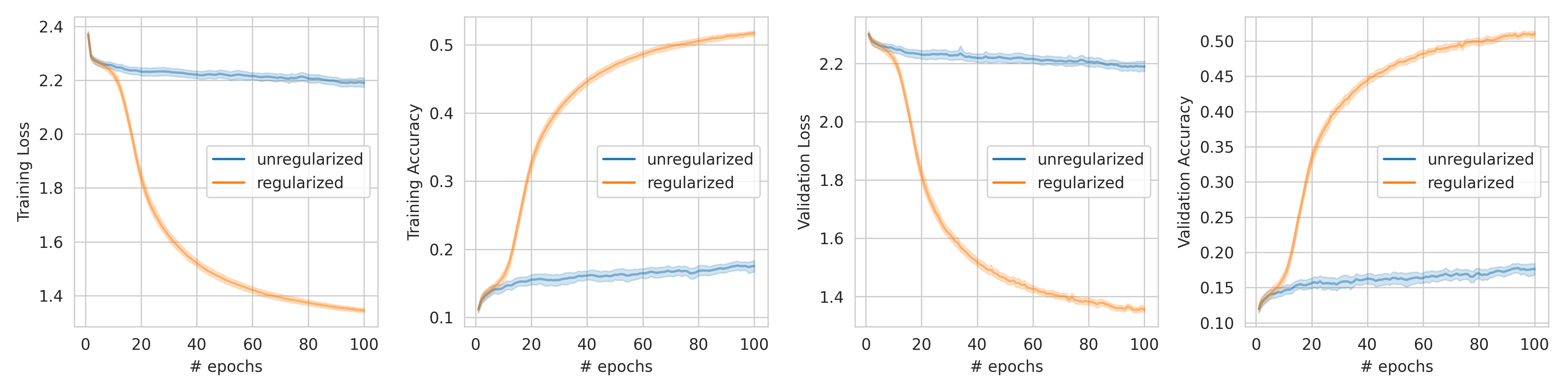
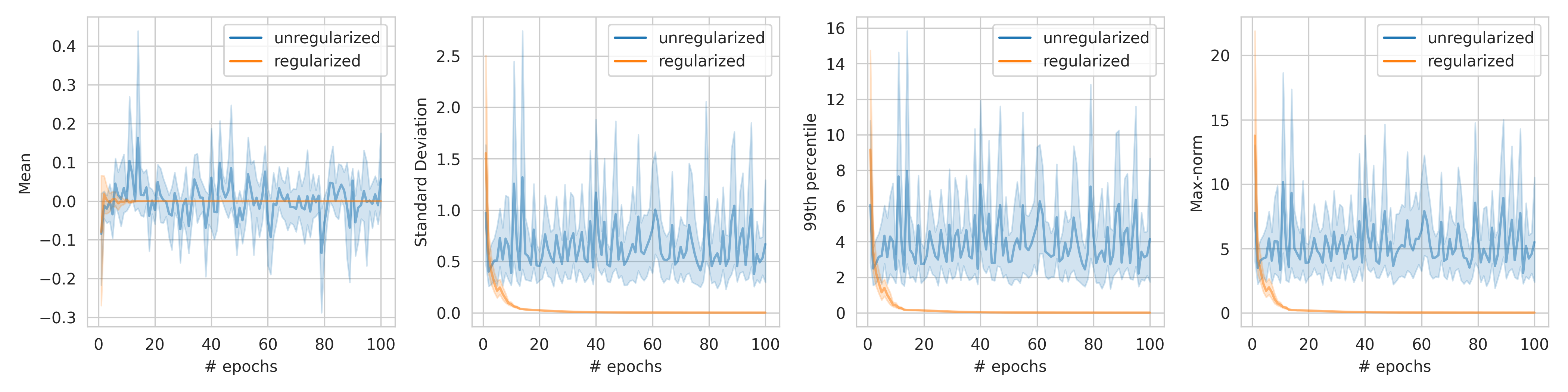
3.2 Many-Layers regime

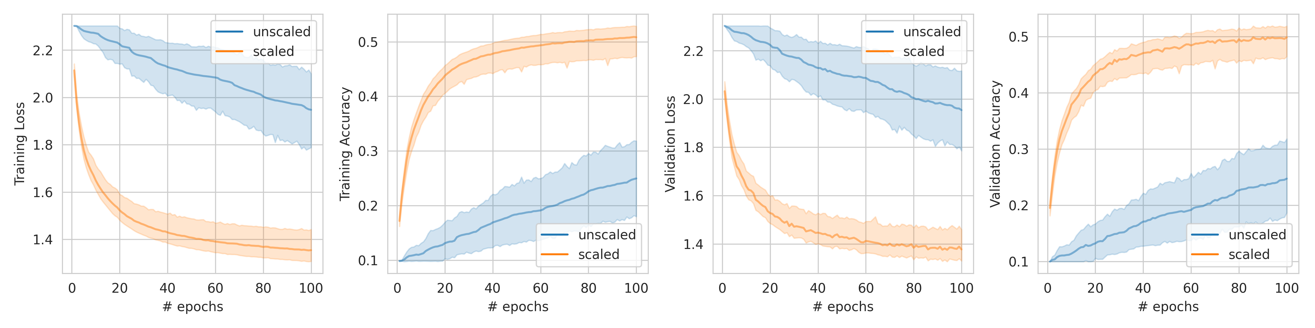
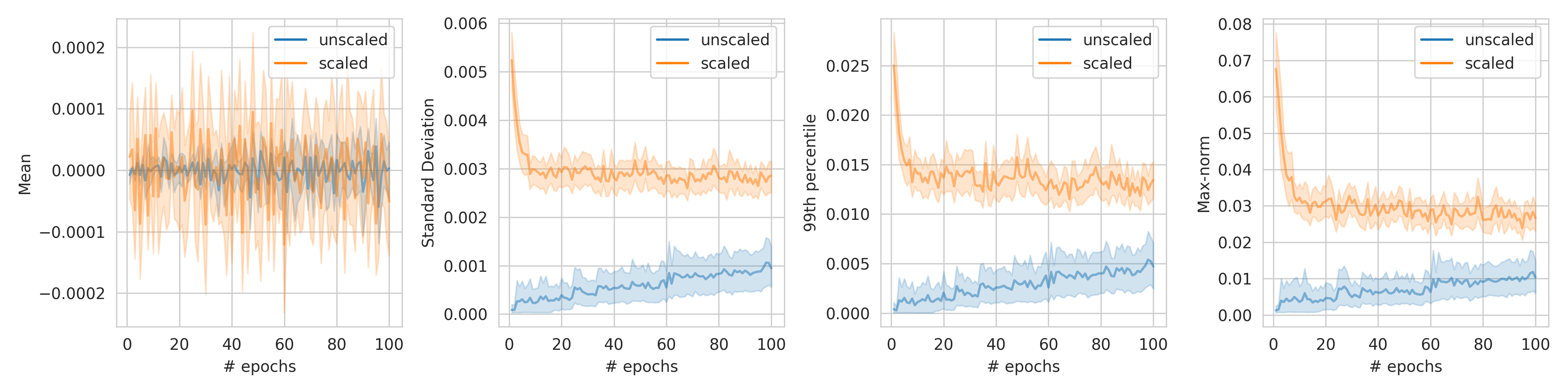
We now demonstrate that the scaling trick can avoid vanishing gradients in the many-layers regime. The network class is specified in Table 2. The table shows that the many-layers regime is modeled, not surprisingly, by stacking many layers. The parameters are initialized based on a centered normal distribution with standard deviation $0.05$. The activations are the same as above. We compare unscaled training (using the standard tanh activation) and scaled training (using α𝛼{\color[rgb]{0,0,0}\definecolor[named]{pgfstrokecolor}{rgb}{0,0,0}\pgfsys@color@gray@stroke{0}\pgfsys@color@gray@fill{0}\alpha}-scaled tanh activation with α=2𝛼2{\color[rgb]{0,0,0}\definecolor[named]{pgfstrokecolor}{rgb}{0,0,0}\pgfsys@color@gray@stroke{0}\pgfsys@color@gray@fill{0}\alpha}=2). Again, we average the results over $25$ runs with different seeds. The resulting accuracy and gradient histories are displayed in Figure 2.

We observe a very similar pattern as in the large-parameters regime: the larger gradients in the beginning (see the bottom panel of the figure) speed up parameter training considerably (see the top panel). The main difference to above is that the improvements kick in immediately (indicating that there are no plateaux from which the algorithm needs to “escape”).

We conclude that the scaling trick can avoid the vanishing-gradient problem, again without leading to an exploding-gradient problem, in the many-layers regime.

Figure 2: accuracies (top) and summary statistics of the coordinate values of the gradients (bottom) in the many-layers regime
Refer to caption
Refer to caption
Figure 3: accuracies (top) and summary statistics of the coordinate values of the gradients (bottom) in the combined regime
Refer to caption
Refer to caption

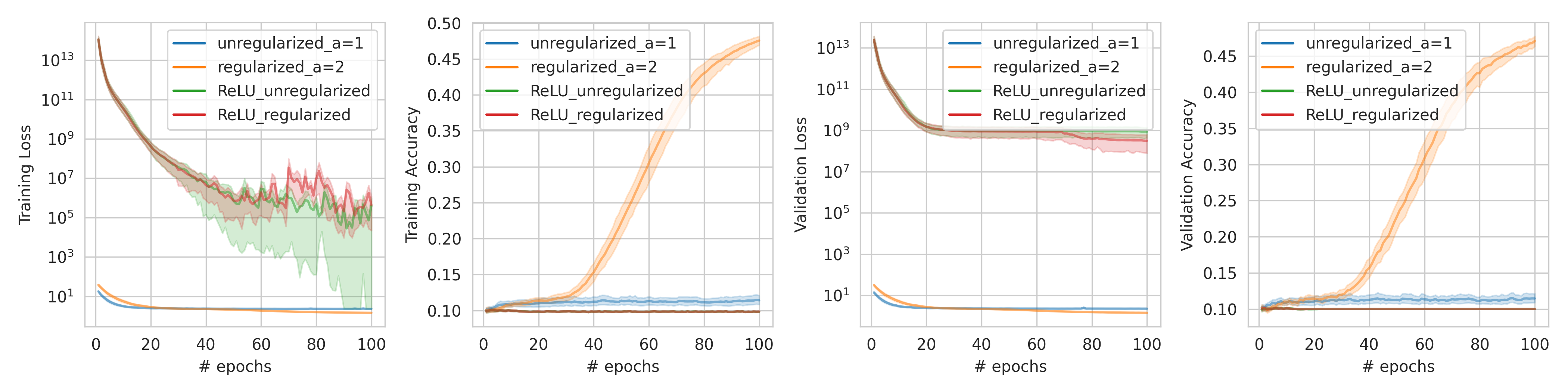
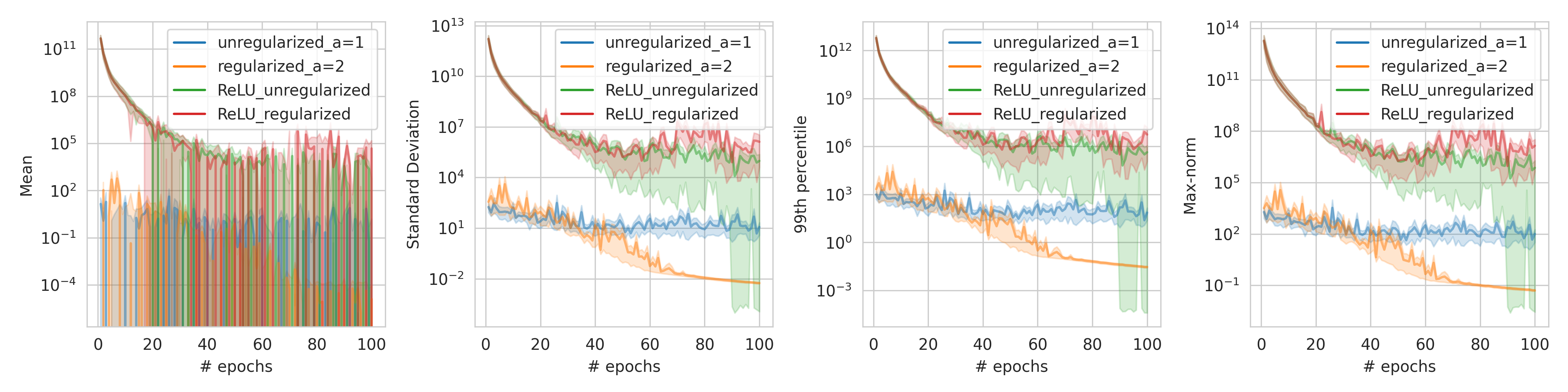
3.3 Combined regime and comparison with relu activation

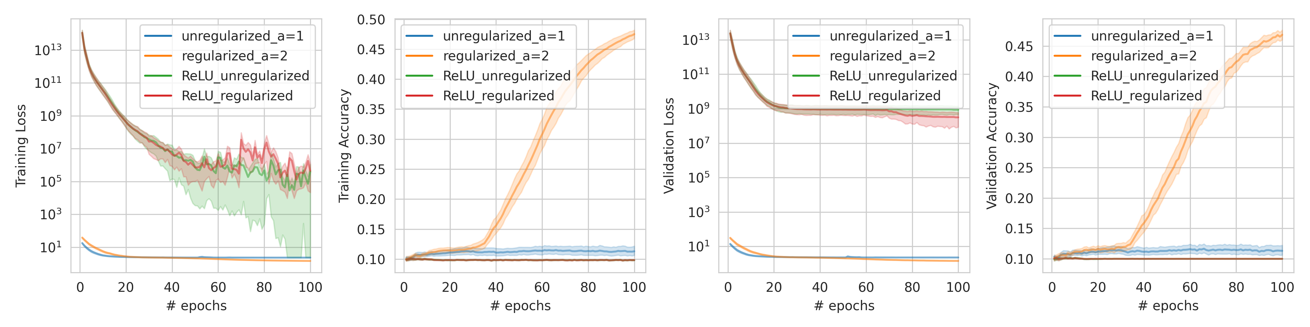
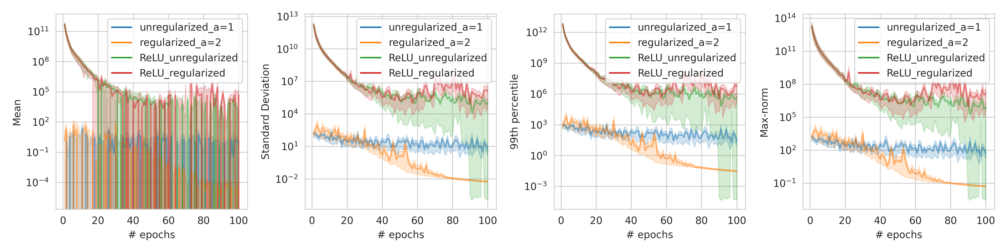
We finally demonstrate that regularization and scaling can be combined. The outline of the model is given in Table 3. The parameters are initialized based on a uniform distribution supported on $[-10,10)$. The activations and the parameters for the regularization and the scaling tricks are the same as above. We compare the standard pipeline with the one that includes regularization and scaling, and we also consider tanh replaced by relu. The results over $25$ runs with different seeds are displayed in Figure 3 (since scaling does not affect relu-type functions, only regularization is mentioned in the relu case). The results here corroborate the results above and show that the two remedies can indeed be combined. An additional observation is that relu, in this specific example, is not performing well.

Table 4 in the Appendix contains the runtimes of one model from the combined regime executed on the same, regular graphics card. It shows that our two remedies do not involve significant computational overhead.

We conclude that our remedies can render tanh robust with respect to the vanishing-gradient problem. Our experiments are not designed to give an overall comparison of different types of activation functions, such as tanh and relu, or even to find the “best” activation function; in fact, which activation function is the “best” one surely depends on the specific settings (architecture, data, parameters, …), the goal (computational efficiency, accuracy, …), and so forth. But what our study is able to show is that sigmoid-type activation is a serious contender.

4 Discussion

The paper provides a fresh look at the vanishing-gradient problem in the context of sigmoid-type activation. In particular, the paper shows that two simple remedies, regularization and rescaling, can avoid the vanishing-gradient problem. This observation suggests that sigmoid-type activation is still a contender in practice.

There are also efforts to study the vanishing- (and exploding-)gradient problems from the perspective of mean-field theory [Sussillo, 2014, Hanin, 2018]. These works currently focus on how network widths and depths relate to vanishing gradients, but it would be interesting to see if their approaches can also yield further theoretical insights into our findings.

For the sake of a clear and concise delivery of the main ideas, we have restricted ourselves to feedforward networks. But we have every reason to believe that our concepts apply much more generally, such as to recurrent neural networks (RNNs) [Kalchbrenner and Blunsom, 2013, Mikolov, 2012], for example. Similarly, the numerical setup focuses on tanh activation, which is currently the most popular sigmoid-type activation, but our remedies also apply to other activation functions, such as softsign activation—cf. [Lederer, 2021, Section 3]—for example. And finally, other types of regularizations, such as $\ell_{1}$-regularization [Alvarez and Salzmann, 2016, Feng and Simon, 2017, Kim et al., 2016], are expected to avoid vanishing gradients similarly as $\ell_{2}$-regularization.

Many questions, however, remain open. In particular, our paper does not yet give a final answer to the question of which activation function to use in a specific setting. But our paper illustrates that an entire class of activation functions might have been underrated, and, on a more general level, it illustrates that conceptual and mathematical research—rather than anecdotal evidence or hearsay—can lead to more informed design choices in practice.

Acknowledgements

We thank Xingtu Liu, Pegah Golestaneh, Mike Laszkiewicz, and Nils Müller for helpful input.

References

  • Alvarez and Salzmann [2016] J. Alvarez and M. Salzmann. Learning the number of neurons in deep networks. In Conference on Neural Information Processing Systems, pages 2270–2278, 2016.
  • Bottou [2010] L. Bottou. Large-scale machine learning with stochastic gradient descent. In Proceedings of COMPSTAT’2010, pages 177–186. Springer, 2010.
  • Feng and Simon [2017] J. Feng and N. Simon. Sparse-input neural networks for high-dimensional nonparametric regression and classification. arXiv:1711.07592, 2017.
  • Glorot and Bengio [2010] X. Glorot and Y. Bengio. Understanding the difficulty of training deep feedforward neural networks. In Proceedings of the Thirteenth International Conference on Artificial Intelligence and Statistics, pages 249–256, 2010.
  • Hanin [2018] B. Hanin. Which neural net architectures give rise to exploding and vanishing gradients? In Conference on Neural Information Processing Systems, pages 582–591, 2018.
  • He et al. [2015] K. He, X. Zhang, S. Ren, and J. Sun. Delving deep into rectifiers: surpassing human-level performance on imagenet classification. In Proceedings of the IEEE International Conference on Computer Vision, pages 1026–1034, 2015.
  • Hebiri and Lederer [2020] M. Hebiri and J. Lederer. Layer sparsity in neural networks. arXiv:2006.15604, 2020.
  • Hochreiter [1991] S. Hochreiter. Untersuchungen zu dynamischen neuronalen Netzen. Diploma, Technische Universität München, 1991.
  • Hochreiter et al. [2001] S. Hochreiter, Y. Bengio, P. Frasconi, and J. Schmidhuber. Gradient flow in recurrent nets: the difficulty of learning long-term dependencies. pages 237–243. A field guide to dynamical recurrent neural networks. IEEE Press, 2001.
  • Huang et al. [2021] S.-T. Huang, F. Xie, and J. Lederer. Tuning-free ridge estimators for high-dimensional generalized linear models. Computational Statistics & Data Analysis, 159:107205, 2021.
  • Ioffe and Szegedy [2015] S. Ioffe and C. Szegedy. Batch normalization: accelerating deep network training by reducing internal covariate shift. In International Conference on Machine Learning, pages 448–456, 2015.
  • Kalchbrenner and Blunsom [2013] N. Kalchbrenner and P. Blunsom. Recurrent continuous translation models. In Conference on Empirical Methods in Natural Language Processing, pages 1700–1709, 2013.
  • Kim et al. [2016] J. Kim, V. Calhoun, E. Shim, and J.-H. Lee. Deep neural network with weight sparsity control and pre-training extracts hierarchical features and enhances classification performance: Evidence from whole-brain resting-state functional connectivity patterns of schizophrenia. Neuroimage, 124:127–146, 2016.
  • [14] A. Krizhevsky, V. Nair, and G. Hinton. Cifar-10 (Canadian Institute for Advanced Research). URL http://www.cs.toronto.edu/~kriz/cifar.html.
  • Lederer [2021] J. Lederer. Activation functions in artificial neural networks: A systematic overview. arXiv:2101.09957, 2021.
  • Martens [2010] J. Martens. Deep learning via Hessian-free optimization. In International Conference on Machine Learning, volume 27, pages 735–742, 2010.
  • Mikolov [2012] T. Mikolov. Statistical language models based on neural networks. PhD thesis, Brno University of Technology, 2012.
  • Mishkin and Matas [2015] D. Mishkin and J. Matas. All you need is a good init. In International Conference on Learning Representations, 2015.
  • Sussillo [2014] D. Sussillo. Random walks: Training very deep nonlinear feed-forward networks with smart initialization. CoRR, abs/1412.6558, 2014.
  • Taheri et al. [2021] M. Taheri, F. Xie, and J. Lederer. Statistical guarantees for regularized neural networks. Neural Networks, 142:148–161, 2021.
  • Tan and Lim [2019] H.-H. Tan and K.-H. Lim. Vanishing gradient mitigation with deep learning neural network optimization. In International Conference on Smart Computing & Communications, pages 1–4, 2019.
  • Vincent et al. [2008] P. Vincent, H. Larochelle, Y. Bengio, and P.-A. Manzagol. Extracting and composing robust features with denoising autoencoders. In International Conference on Machine Learning, pages 1096–1103, 2008.

Appendix A Experimental Details

Here, we provide the tables about the architectures as mentioned in the experimental section.

Table 1: neural-network architecture for the large-parameters regime
Layer Output dimensions Filters
Input $(32,32,3)$
3-by-3 convolution $(32,32,3)$ 36
Max pooling $(16,16,3)$ 0
3-by-3 convolution $(16,16,3)$ 36
Max pooling $(8,8,3)$ 0
3-by-3 convolution $(8,8,3)$ 36
Max pooling $(4,4,3)$ 0
Dense $(8)$ 392
Dense $(10)$ 90
Table 2: neural-network architecture for the many-layers regime
Layer Output dimensions Filters
Input $(32,32,3)$
3-by-3 convolution $(32,32,3)$ 3
Max pooling $(16,16,3)$ 3
3-by-3 convolution $(16,16,3)$ 3
Max pooling $(8,8,3)$ 3
3-by-3 convolution $(8,8,3)$ 3
Max pooling $(4,4,3)$ 3
Dense $(8)$ 384
Dense $(8)$ 64
Dense $(8)$ 64
Dense $(8)$ 64
Dense $(10)$ 80
Table 3: neural-network architecture for the combined regime
Layer Output dimensions Filters
Input $(32,32,3)$
3-by-3 convolution $(32,32,3)$ 3
Max pooling $(16,16,3)$ 3
3-by-3 convolution $(16,16,3)$ 3
Max pooling $(8,8,3)$ 3
3-by-3 convolution $(8,8,3)$ 3
Max pooling $(4,4,3)$ 3
Dense $(8)$ 384
Dense $(8)$ 64
Dense $(8)$ 64
Dense $(10)$ 80

Appendix B Runtimes

Here, we provide the table about the runtime as mentioned in the experimental section.

Table 4: comparison of runtimes
Model Runtime (s)
tanh unregularized and unscaled $1057.8$
tanh regularized and scaled $1385.2$
relu unregularized $986.8$
relu regularized $1339.1$

Appendix C Other Sigmoid-Type Activations

In the main part of the paper, we have focused on tanh activation. But we have also mentioned that our results can be transferred readily to other sigmoid-type activation. For illustration, we provide an analog of Figure 3 for the case of tanh replaced by logsigmoid. We obtain virtually the same results as before.

Figure 4: accuracies (top) and summary statistics of the coordinate values of the gradients (bottom) in the combined regime with tanh replaced by logsigmoid  activation
Refer to caption
Refer to caption