State Estimation in Unobservable Power Systems via Graph Signal Processing Tools

Abstract

We consider the problem of estimating the states in an unobservable power system. To this end, we propose novel graph signal processing (GSP) methods. For simplicity, we start with analyzing the DC power flow (DC-PF) model and then extend our algorithms to the AC power flow (AC-PF) model. The main assumption behind the proposed GSP approach is that the grid states, which include the vector of phases and the vector of the magnitudes of the voltages in the system, is a smooth graph signal with respect to the system admittance matrix that represents the underlying graph. Thus, the first step in this paper is to validate the graph-smoothness assumption of the states, both empirically and theoretically. Then, we develop the regularized GSP weighted least squares (GSP-WLS) state estimator, which does not require observability of the network. We propose a sensor placement strategy that aims to optimize the estimation performance of the GSP-WLS estimator. Finally, we extend the GSP-WLS estimator method to the AC-PF model by integrating a smoothness regularization term into the Gauss-Newton algorithm. Numerical results on the IEEE 118-bus system demonstrate that the new GSP methods outperform commonly-used estimation approaches and are robust to missing data.

I Introduction

Power system state estimation (PSSE) is a critical component of modern Energy Management Systems (EMSs) for multiple purposes, including monitoring, analysis, security, control, and management of the power delivery [1]. The PSSE is conducted using topological information, power measurements, and physical constraints [2] to estimate the voltages (states) at the system buses. The performance and reliability of the PSSE largely depend on the availability and the quality of the measurements [3]. However, there are various realistic scenarios where the system is unobservable, that is, the number of sensors is not sufficiently large or sensors are not well placed in the network. In addition, a system may become unobservable due to communication errors, topology changes, sensor failures [1], malicious attacks [4, 5, 6], and electrical blackouts [7]. A direct implication of system unobservability is that estimators that assume deterministic states, such as the commonly-used weighted least-squares (WLS) estimator, can no longer be used since they are inaccurate, inconsistent, and may have large estimation errors even in the absence of noise [8, 9]. Therefore, developing new estimation methods that enable the full functionality of unobservable systems is crucial for reliable operation of the power grid.

State estimation in unobservable systems must incorporate additional properties or information beyond the power flow equations in order to obtain a meaningful estimation. Most existing approaches are two-step solutions that first produce additional pseudo-measurements, e.g. based on short-term load forecasting, to make the system observable, and then estimate the states by any existing technique [10, 11, 12, 13]. However, pseudo-measurements do not contain real-time data and thus, result in an inaccurate estimation. Dynamic state estimation utilizes measurements at different time instants [13, 14], but need fast scan rates to capture the dynamics and are based on restrictive stationary system assumptions [13]. PSSE that uses data from smart meters and phasor measurement units (PMUs) to overcome observability issues [15, 8, 16] is usually inapplicable due to the limited deployment of these sensors [17], their investment cost, and the computational complexity of these approaches [18]. Sparse signal recovery methods [19] use matrix completion to estimate the states under low-observability conditions. However, to employ the matrix completion framework, the measurements matrix should be a low-rank matrix. Unfortunately, this assumption is system-dependent and does not always hold due to, e.g. the spatial correlation between loads at neighboring buses. Deep-learning techniques have been recently used for pseudo-measurement generation and for reconstructing missing data for PSSE [17, 20]. However, the success of these techniques heavily depends on the availability of numerous high-quality event labels that are rarely available in practice [21]. In addition, some of these methods do not utilize the physical model [17], which may result in poor performance in physical systems.

In this paper, we consider the use of graph signal processing (GSP) tools for state estimation in unobservable systems. A power system can be represented as an undirected weighted graph, where the nodes (vertices) of the graph are the grid buses and its edges are the transmission lines. In the literature, several works have used concepts from graph theory and graphical models in power systems for sensor placement [22], topology identification [23, 24, 25], state estimation [26, 27, 4], analysis [28, 29], and optimal power flow calculation [30, 31]. However, the graphical model methods assume a specific statistical structure, which does not necessarily apply in power systems, and often do not use the physical models, which may result in poor performance in practice. GSP is a new and emerging field that extends concepts and techniques from traditional digital signal processing (DSP) to data on graphs. GSP theory includes methods such as the Graph Fourier Transform (GFT), graph filters [32, 33, 34], and sampling and recovery of graph signals [35, 36]. Recent works propose the integration of GSP in power systems, such as the GSP framework for the power grid based on PMU data in [37], the spectral graph analysis of power flows in [38], and false-data injection (FDI) attacks detection by GSP in [5]. However, state estimation without observability by GSP tools has not been demonstrated before.

In this paper, we develop GSP methods for state estimation in power systems based on interpreting the voltage phases and magnitudes as graph signals. First, we show that the states for static PSSE, that may include both the phases and the magnitudes of the voltages, are smooth graph signals with respect to (w.r.t.) the nodal admittance matrix, which is a Laplacian matrix in the graph representation of the network. Second, we develop a GSP-WLS estimation method for PSSE in the DC power flow (DC-PF) model that uses the smoothness of the states. The GSP-WLS estimator does not require observability of the network, is only based on the current-time measurements, and does not assume a specific structure of the correlations between the buses. We also introduce a new approach for sensor placement that optimizes the estimation performance obtained by the GSP-WLS estimator. It should be noted that we initially treat a simplistic PSSE in the DC-PF model in order to simplify the presentation and the derivation of the estimation and sensor allocation methods. Then, we extend our estimation method to the more realistic AC-PF model by developing a regularized Gauss-Newton method for PSSE that uses the smoothness of the phases and magnitudes of the voltages. Numerical simulations validate the merit of the new estimators under different setups.

The rest of this paper is organized as follows. In Section II we introduce GSP background, the model, and the conventional estimation approach. In Section III we study the GSP properties of the states. In Section IV we derive the GSP-WLS state estimator for the DC-PF model and a sensor placement method that aims to optimize the estimation performance. In Section V we extend our estimation method to the AC-PF model by deriving the regularized Gauss-Newton method for state estimation. A simulation study is presented in Section VI and the conclusion appears in Section VII.

In the rest of this paper, vectors and matrices are denoted by boldface lowercase letters and boldface uppercase letters, respectively. The notations $(\cdot)^{T}$, $(\cdot)^{-1}$, $(\cdot)^{\dagger}$ and $\text{Tr}(\cdot)$ denote the transpose, inverse, Moore-Penrose pseudo-inverse, and trace operators, respectively. The $m$th element of the vector ${\bf{a}}$ and the $(m,q)$th element of the matrix ${\bf{A}}$ are denoted by $a_{m}$ and $A_{m,q}$, respectively. Similarly, ${\bf{A}}_{\mathcal{S}_{1},\mathcal{S}_{2}}$ denotes the submatrix of ${\bf{A}}$ whose rows and columns are indexed by the sets $\mathcal{S}_{1}$ and $\mathcal{S}_{2}$, where ${\bf{A}}_{\mathcal{S}}\stackrel{{\scriptstyle\triangle}}{{=}}{\bf{A}}_{\mathcal{S},\mathcal{S}}$, and ${\bf{a}}_{\mathcal{S}}$ is a subvector of ${\bf{a}}$ containing the elements indexed by $\mathcal{S}$. The gradient of a vector function ${\bf{g}}({\bf{x}})\in\mathbb{R}^{K}$ w.r.t. ${\bf{x}}\in\mathbb{R}^{M}$, $\frac{\partial{\bf{g}}({\bf{x}})}{\partial{\bf{x}}}$, is a matrix in $\mathbb{R}^{K\times M}$, with the $(k,m)$th element equal to $\frac{\partial g_{k}}{\partial x_{m}}$. The matrices ${\bf{I}}$ and ${\bf{0}}$ denote the identity matrix and the zero matrix with appropriate dimensions, respectively, and $||\cdot||$ denotes the Euclidean $l_{2}$-norm of vectors. For a vector ${\bf{a}}$, ${\text{diag}}({\bf{a}})$ is a diagonal matrix whose $n$th diagonal entry is $a_{n}$.

II Background and Model

In this section, we first present the background on the theory of GSP in Subsection II-A. Then, we present the considered power-flow measurement model, as well as the state estimation and network observability for this model, in Subsection II-B.

II-A Background: GSP framework

Let ${\mathcal{G}}({\mathcal{V}},\xi)$ be a general undirected weighted graph, where ${\mathcal{V}}=\{1,\ldots,N\}$ and ${\xi}=\{1,\ldots,P\}$ are the sets of nodes and edges, respectively. The matrix ${\bf{W}}\in{\mathbb{R}}^{N\times N}$ is the weighted adjacency matrix of the graph $\mathcal{G}({\mathcal{V}},\xi)$, where $W_{k,n}$ denotes the weight of the edge between node $k$ and node $n$. We assume that $W_{k,n}\geq 0$ and that $W_{k,n}=0$ if no edge exists between $k$ and $n$. The graph Laplacian matrix is defined as

$$L_{k,l}=\begin{cases}\displaystyle\sum\nolimits_{n=1}^{N}W_{k,n},&k=l\\ \displaystyle-W_{k,l},&{\text{otherwise}}\end{cases},~{}~{}~{}k,l=1,\ldots,N.$$ (1)

The Laplacian matrix, ${\bf{L}}$, is a real and positive semidefinite matrix with the eigenvalue-eigenvector decomposition

$${\bf{L}}={\bf{V}}{\bf{\Lambda}}{\bf{V}}^{T},$$ (2)

where the columns of ${\bf{V}}$ are the eigenvectors of ${\bf{L}}$, ${\bf{V}}^{T}={\bf{V}}^{-1}$, and ${\bf{\Lambda}}\in{\mathbb{R}}^{N\times N}$ is a diagonal matrix consisting of the ordered eigenvalues of ${\bf{L}}$: $0=\lambda_{1}<\lambda_{2}\leq\ldots\leq\lambda_{N}$. By analogy to the frequency of signals in DSP, the Laplacian eigenvalues, $\lambda_{1},\ldots,\lambda_{N}$, can be interpreted as the graph frequencies, and the eigenvectors in ${\bf{V}}$ can be interpreted as the corresponding graph frequency components. Together they define the spectrum of the graph ${\mathcal{G}}({\mathcal{V}},\xi)$ [34].

A graph signal is a function that resides on a graph, assigning a scalar value to each node, and is an $N$-dimensional vector. The GFT of a graph signal ${\bf{a}}$ w.r.t. the graph ${\mathcal{G}}({\mathcal{V}},\xi)$ is defined as [34, 32]:

$$\tilde{{\bf{a}}}\triangleq{\bf{V}}^{-1}{\bf{a}}.$$ (3)

Similarly, the inverse GFT is obtained by left multiplication of a vector by ${\bf{V}}$. The Dirichlet energy of a graph signal, ${\bf{a}}$, is defined as

$${\mathcal{E}}_{{\bf{L}}}({\bf{a}})\stackrel{{\scriptstyle\triangle}}{{=}}{{\bf{a}}^{T}}{\bf{L}}{\bf{a}} = \frac{1}{2}\mathop{\sum}_{k=1}^{N}\sum_{n=1}^{N}W_{k,n}\big{(}a_{k}-a_{n}\big{)}^{2}$$ (4)

$$= \sum_{k=1}^{N}\lambda_{k}\tilde{a}_{k}^{2},$$ (5)

where the second equality is obtained by substituting (1) and the last equality is obtained by substituting (2) and (3).

The Dirichlet energy from (4) and (5) is a smoothness measure, which is used in graphs to quantify the variability encoded by the graph weights [34]. A graph signal, ${\bf{a}}$, is smooth if

$${\mathcal{E}}_{{\bf{L}}}({\bf{a}})\leq\varepsilon,$$ (6)

where $\varepsilon$ is small in terms of the specific application [34]. It can be seen that the smoothness condition in (6) requires connected nodes to have similar values (according to (4)) and forces the graph spectrum of the graph signal to be concentrated in the small eigenvalues region (according to (5)).

A graph filter applied on a graph signal is a linear operator that satisfies the following [33]:

$${\bf{a}}_{out}={\bf{V}}{\text{diag}}(\psi(\lambda_{1}),\dots,\psi(\lambda_{N})){\bf{V}}^{T}{\bf{a}}_{in},$$ (7)

where ${\bf{a}}_{out}$ and ${\bf{a}}_{in}$ are the output and input graph signals, and $\psi(\lambda_{n})$ is the graph filter frequency response at the graph frequency $\lambda_{n}$, $n=1,\ldots,N$. Low-pass graph filters of order $K$ are defined as follows [39].

Definition 1

The graph filter in (7) is a low-pass graph filter of order $K$ with a cutoff frequency at $\lambda_{K}$ if $\eta_{K}<1$, where

$${\eta}_{k}\stackrel{{\scriptstyle\triangle}}{{=}}\frac{\max\{|{\psi}({\lambda}_{k+1})|,\ldots,|{\psi}({\lambda}_{N})|\}}{\min\{|{\psi}({\lambda}_{1})|,\ldots,|{\psi}({\lambda}_{k})|\}},~{}k=1,\ldots,N-1.$$ (8)

This definition implies that if $\eta_{K}<1$, then most of the energy of the graph filter is concentrated in the first $K$ frequency bins of the graph filter [39]. Upon passing a graph signal through ${\bf{V}}{\text{diag}}(\psi(\lambda_{1}),\dots,\psi(\lambda_{N})){\bf{V}}^{T}$, the high-frequency components (related to graph frequencies greater than $\lambda_{K}$) are attenuated relative to the low-frequency components (related to graph frequencies lower than $\lambda_{K}$). Thus, as long as the input of the filter is a “well-behaved” excitation and does not possess strong high-pass components, the output signal is a $K$-low-pass graph signal [39], and, thus, a smooth graph signal for small $K$, as defined in (6).

II-B DC-PF model: state estimation and observability

A power system is a network of buses (generators or loads) connected by transmission lines that can be represented as an undirected weighted graph, ${\mathcal{G}}({\mathcal{V}},\xi)$, where the set of nodes, $\mathcal{V}$, is the set of $N$ buses and the edge set, $\xi$, is the set of $P$ transmission lines between these buses. We denote the set of all sensor measurements by $\mathcal{M}$, which includes $M\stackrel{{\scriptstyle\triangle}}{{=}}2P+N$ active power measurements at the $N$ buses and at the bi-directional $P$ transmission lines. According to the $\pi$-model [1], each transmission line, $(k,n)\in\xi$, which connects buses $k$ and $n$, is characterized by an admittance value, $Y_{k,n}$.

The active power and the voltages obey multivariate versions of Kirchhoff’s and Ohm’s laws that result in the nonlinear equations of the AC-PF model (see Section V). In order to analyze the GSP properties and to simplify the presentation of the new methods, we first approximate these equations by the DC-PF model [1], in which the states are the voltage angles. Therefore, we consider first a DC-PF model with the following noisy measurements of the active power [1]:

$${\bf{z}}={\bf{H}}{\mbox{\boldmath$\theta$}}+{\bf{e}},$$ (9)

where

• ${\bf{z}}=[z_{1},\dots,z_{M}]^{T}\in{\mathbb{R}}^{M}$ is the active power vector.

• ${\mbox{\boldmath$\theta$}}=[\theta_{1},\dots,\theta_{N}]^{T}\in{\mathbb{R}}^{N}$ is the system state vector, where $\theta_{n}$ is the voltage angle at bus $n$. In low-observable systems, it is more convenient to delay the assignment of the reference angle (p. 165 in [3]). Thus, $\theta$ includes the angle of the reference bus.

• ${\bf{e}}\in{\mathbb{R}}^{M}$ is zero-mean Gaussian noise with covariance ${\bf{R}}$.

• ${\bf{H}}\in{\mathbb{R}}^{M\times N}$ is the measurements matrix, which is determined by the topology of the network, the susceptance of the transmission lines, and the meter locations [4]. In particular, the $N$ rows of ${\bf{H}}$ associated with the meters on the buses that measure the total power flow on transmission lines connected to these buses create together the nodal admittance matrix (see, e.g. p. 97 in [3]), ${\bf{B}}$. ${\bf{B}}$ has the following $(k,l)$-th element:

  $$B_{k,l}=\begin{cases}\displaystyle\sum_{n\in{\mathcal{N}}_{k}}-b_{k,n},&k=l\\ \displaystyle b_{k,l},&(k,l)\in\xi\\ \displaystyle 0,&\text{otherwise}\end{cases},~{}\forall k,l=1,\ldots,N,$$ (10)

  where ${\mathcal{N}}_{k}$ is the set of buses connected to bus $k$ and $b_{k,n}<0$ is the susceptance of $(k,n)\in\xi$, i.e. $b_{k,n}={\text{Im}}\{Y_{k,n}\}$.

The goal of DC-PF PSSE is to recover the state vector, $\theta$, from the measurements vector, ${\bf{z}}$, for various monitoring purposes [1, 27]. Since $\theta$ also includes the reference bus, without loss of generality, we constrain the angle of bus $1$ (the reference bus) to be $\theta_{1}=0$. The PSSE in this case is implemented by using the measurements described in (9) and the following WLS estimator [1]:

$$\begin{array}[]{lr}\hat{{\mbox{\boldmath$\theta$}}}{}^{\text{WLS}}=\arg\min\limits_{{\mbox{\boldmath{\scriptsize$\theta$}}}\in\mathbb{R}^{N}}({\bf{z}}-{{\bf{H}}}{{\mbox{\boldmath$\theta$}}})^{T}{\bf{R}}^{-1}({\bf{z}}-{{\bf{H}}}{{\mbox{\boldmath$\theta$}}})\\ {\text{ such that }}\theta_{1}=0.\end{array}$$ (13)

The solution of (13) is

$$\left\{\begin{array}[]{l}\hat{{\mbox{\boldmath$\theta$}}}{}_{\bar{\mathcal{V}}}^{\text{WLS}}={\bf{K}}{\bf{z}}\\ \hat{\theta}_{1}^{\text{WLS}}=0\end{array}\right.,$$ (16)

where

$${\bf{K}}\stackrel{{\scriptstyle\triangle}}{{=}}({\bf{H}}_{\mathcal{M},\bar{\mathcal{V}}}^{T}{\bf{R}}^{-1}{\bf{H}}_{\mathcal{M},\bar{\mathcal{V}}})^{-1}{\bf{H}}_{\mathcal{M},\bar{\mathcal{V}}}^{T}{\bf{R}}^{-1}$$ (17)

and $\bar{\mathcal{V}}\stackrel{{\scriptstyle\triangle}}{{=}}\mathcal{V}\setminus 1$ is the set of all buses except the reference bus.

For state estimation to be feasible, we need to have enough measurements such that the system state can be uniquely determined by the WLS estimation approach. This observability requirement, before the assignment of reference angles, can be defined by one of the following (p. 165 in [3]).

Definition 2

Assume the DC-PF model from (9). The network is observable if any matrix that is obtained from ${\bf{H}}$ by deleting one of its columns has a full column rank of $N-1$.

Definition 3

The network is observable if the following holds: ${\bf{H}}{\mbox{\boldmath$\theta$}}={\bf{0}}$ if and only if ${\mbox{\boldmath$\theta$}}=\alpha{\mathbf{1}}$, where $\alpha$ is an arbitrary scalar.

In particular, since according to Definition 2 ${\bf{H}}_{\mathcal{M},\bar{\mathcal{V}}}$ has full column rank for an observable system, observability ensures that ${\bf{H}}_{\mathcal{M},\bar{\mathcal{V}}}^{T}{\bf{R}}^{-1}{\bf{H}}_{\mathcal{M},\bar{\mathcal{V}}}$ is non-singular, and the WLS estimator from (16)-(17) is well-defined for any observable network.

In practice, however, network observability is not always guaranteed. In such cases, the WLS estimator from (16) cannot be implemented. Even for observable systems, errors and outliers may have a disastrous effect on the state estimation. In the following, we show that incorporating graphical information by using GSP tools improves the state estimation performance and enables estimation even in unobservable systems.

III GSP properties of the states

The power system can be represented as an undirected weighted graph, ${\mathcal{G}}({\mathcal{V}},\xi)$, as described at the beginning of Subsection II-B. In this context, the state vector, ${\mbox{\boldmath$\theta$}}\in{\mathbb{R}}^{N}$, and the subvector of ${\bf{z}}$ from (9) that contains the $N$ active power injection measurements at the $N$ buses, denoted as ${\bf{z}}_{\text{bus}}$, can be interpreted as graph signals. In this graph representation, the nodal admittance matrix from (10) is a Laplacian matrix:

$${\bf{L}}={\bf{B}}.$$ (18)

In this section, we establish the graph low-pass nature and the smoothness of the state vector in power systems under normal operation conditions and where the Laplacian matrix is set to be the nodal admittance matrix, as defined in (18). That is, by using the smoothness defined in (4)-(6), we show that

$${\mathcal{E}}_{{\bf{L}}}({\mbox{\boldmath$\theta$}})={{\mbox{\boldmath$\theta$}}^{T}}{\bf{L}}{\mbox{\boldmath$\theta$}}\leq\varepsilon,$$ (19)

where $\varepsilon$ is small relative to the other parameters in the system. These results are consistent with the low-pass graph nature of the complex voltages in the AC-PF model, described in [37].

III-A Theoretical validation - Output of a low-pass graph filter

First, we show analytically that the state vector is a low-pass graph signal. By substituting (18) in the model in (9), after taking only the active power injection measurements we obtain

$${\bf{z}}_{\text{bus}}={\bf{L}}{\mbox{\boldmath$\theta$}}+{\bf{e}}_{\text{bus}},$$ (20)

where ${\bf{e}}_{\text{bus}}$ contains the elements of the noise vector, ${\bf{e}}$, that are related to the $N$ power measurements at the $N$ buses. Equation (20) implies that since ${\bf{L}}$ is a Laplacian matrix, it satisfies ${\bf{L}}{\bf{1}}={\bf{0}}$ [40], where ${\bf{1}}$ is the a vector of ones with appropriate dimensions. Thus, we can recover the states from (20) up-to-a-constant shift, which can be written as

$$\theta = {\bf{L}}^{\dagger}\left({\bf{z}}_{\text{bus}}-{\bf{e}}_{\text{bus}}\right)+c_{1}{\bf{1}}$$ (21)

$$= {\bf{V}}{\bf{\Lambda}}^{\dagger}{\bf{V}}^{T}\left({\bf{z}}_{\text{bus}}-{\bf{e}}_{\text{bus}}\right)+c_{1}{\bf{1}},$$

where $c_{1}$ is an arbitrary constant that represents the constant-invariant property of the state vector [1, 41] and the last equation is obtained by substituting (2). Without loss of generality, we choose the value of $c_{1}$ to be

$$c_{1}=c_{2}{\bf{1}}^{T}\left({\bf{z}}_{\text{bus}}-{\bf{e}}_{\text{bus}}\right),$$ (22)

where $c_{2}$ is an arbitrary constant. Using (22) and the definition of the pseudo-inverse operator, the model in (21) can be written as the following linear graph-filter input-output model:

$${\mbox{\boldmath$\theta$}}={\bf{V}}{\text{diag}}(\psi(\lambda_{1}),\dots,\psi(\lambda_{N})){\bf{V}}^{T}\left({\bf{z}}_{\text{bus}}-{\bf{e}}_{\text{bus}}\right),$$ (23)

where

$$\psi(\lambda_{n})=\left\{\begin{array}[]{lr}\frac{1}{\lambda_{n}},&n=2,\ldots,N\\ Nc_{2},&n=1\end{array}\right..$$ (24)

That is, $\theta$ is an output of a graph filter with the graph frequency response in (24). This graph-filter representation holds under the assumption that the network is connected. Thus, $\lambda_{1}$ is the only zero eigenvalue of ${\bf{L}}$ with the associated eigenvector $\frac{1}{\sqrt{N}}{\bf{1}}$ [40].

Since the eigenvalues of ${\bf{L}}$ are ordered, $0=\lambda_{1}<\lambda_{2}\leq\lambda_{3}\leq\ldots\leq\lambda_{N}$, it can be seen that the graph frequency response in (24) decreases as $n$ increases, as long as $c_{2}>\frac{1}{N\lambda_{2}}$. By substituting (24) in (8), we obtain

$${\eta}_{k}=\left\{\begin{array}[]{lr}\frac{\lambda_{k}}{{\lambda}_{k+1}},&2\leq k\leq N-1\\ \frac{1}{Nc_{2}\lambda_{2}},&k=1\end{array}\right.,$$ (25)

where $\eta_{k}<1$, $k=2,\ldots,N-1$. By choosing $c_{2}>>\frac{1}{N\lambda_{2}}$, we obtain that ${\eta}_{1}<<1$. Thus, according to Definition 1, ${\bf{V}}{\text{diag}}(\psi(\lambda_{1}),\dots,\psi(\lambda_{N})){\bf{V}}^{T}$ in (23) is a graph low-pass filter of any order $K\geq 1$. Since ${\bf{z}}_{\text{bus}}$ in (21) includes the generated powers and loads, it can be assumed to be random [42, 43], and thus, the input signal, ${\bf{z}}_{\text{bus}}-{\bf{e}}_{\text{bus}}$, does not possess strong high-pass components. Thus, as explained after Definition 1, the state vector $\theta$ is a first-order low-pass graph signal, and a smooth graph signal, as defined in (19).

III-B Experimental validation in IEEE systems

In the following, we demonstrate the smoothness of the state signal in the graph spectrum domain for the IEEE test case systems [44]. We also demonstrate the smoothness of the voltage magnitude vector, ${\bf{v}}\stackrel{{\scriptstyle\triangle}}{{=}}[|v_{1}|,\dots,|v_{N}|]^{T}$, which can be interpreted as graph signals, that will be used in Section V along with the AC-PF model. In Fig. 1 we compare between the normalized state vector, $\frac{{\mbox{\boldmath{\scriptsize$\theta$}}}}{||{\mbox{\boldmath{\scriptsize$\theta$}}}||}$, and its GFT (calculated by using (3)), $\frac{\tilde{{\mbox{\boldmath{\scriptsize$\theta$}}}}}{||\tilde{{\mbox{\boldmath{\scriptsize$\theta$}}}}||}$, versus bus or spectral indices, for the IEEE 118-bus system [44]. Similarly, in Fig. 2 we present the normalized voltage magnitude vector, $\frac{{\bf{v}}}{||{\bf{v}}||}$, and its GFT, $\frac{\tilde{{\bf{v}}}}{||\tilde{{\bf{v}}}||}$, and in Fig. 3 we present the normalized power vector, $\frac{{\bf{z}}_{\text{bus}}}{||{\bf{z}}_{\text{bus}}||}$, and its GFT, $\frac{\tilde{{\bf{z}}}_{\text{bus}}}{||\tilde{{\bf{z}}}_{\text{bus}}||}$. For the sake of clarity, the vectors in Figs. 1-3 have been decimated by a factor of $3$.

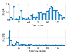
Figure 1: The state vector (top) and its GFT (bottom) for IEEE 118-bus system.

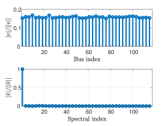
Figure 2: The voltage magnitude vector (top) and its GFT (bottom) for IEEE 118-bus system.

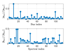
Figure 3: The active power measurements vector (top) and its GFT (bottom) for IEEE 118-bus system.

It can be seen that most of the energy of the state signal, i.e. the phases (Fig. 1) and the magnitudes (Fig. 2) of the voltages, is concentrated in the low graph frequencies region. Thus, we can conclude that the state vector and the voltage magnitude vector are smooth graph signals in the sense of (5). In contrast, the energy of the power injection measurements vector (Fig. 3) is uniformly distributed across all graph frequencies. Thus, the power signal cannot considered to be smooth. Similar results were obtained for other IEEE systems.

Next, we validate experimentally that the states, $\theta$, and the magnitudes, ${\bf{v}}$, are significantly smoother than the power vector, ${\bf{z}}_{\text{bus}}$, by comparing their associated normalized Dirichlet energy for typical IEEE systems in Table I. The values of the Laplacian (nodal admittance) matrix, ${\bf{L}}={\bf{B}}$, the voltages, and the power data are taken from [44]. It can be seen that the phases and magnitudes are much smoother than the power injection vectors. This result is reasonable since the phase differences between connected buses are small under normal conditions and the magnitudes are approximately constant [27], while the power may be very different since each generator/load injects different power into the system.

	IEEE test-case system
Measure	14-bus	30-bus	57-bus	118-bus	300-bus
$\frac{{\mathcal{E}}_{{\bf{L}}}({\mbox{\boldmath{\scriptsize$\theta$}}})}{||{\mbox{\boldmath{\scriptsize$\theta$}}}||^{2}}$	0.6617	0.3015	0.3714	1.1740	1.2371
$\frac{{\mathcal{E}}_{{\bf{L}}}({\bf{v}})}{||{\bf{v}}||^{2}}$	0.0036	0.0022	0.008	0.0082	0.0199
$\frac{{\mathcal{E}}_{{\bf{L}}}({\bf{z}}_{\text{bus}})}{||{\bf{z}}_{\text{bus}}||^{2}}$	16.4079	18.3307	50.8035	56.1047	138.8024

TABLE I: Normalized smoothness values of IEEE systems.

IV GSP-WLS estimator in DC-PF model

The recovery of smooth graph signals by incorporating regularization terms has been well studied in the GSP literature [45, 33] and in the context of Laplacian regularization [46, 47]. In this section, we cast the state estimation problem as a regularized graph signal recovery problem. In particular, we exploit the smoothness of the state vector, established in Section III, to develop the smoothness-based regularized GSP-WLS estimator of the states in Subsection IV-A. We discuss the properties of the proposed approach in Subsection IV-B, where its main advantage is that it does not require system observability. In Subsection IV-C we introduce a by-product of this approach: an estimator of the missing power data. Finally, in Subsection IV-D we design a sensor allocation policy that aims to optimize the performance of the GSP-WLS estimator.

IV-A GSP-WLS estimator for partial measurement model

In the following, we consider the case where only partial observations of the signal ${\bf{z}}$ from (9) are available over a subset of sensors from ${\mathcal{M}}$, where this subset is denoted by $\mathcal{S}$ and $\mathcal{S}\subseteq{\mathcal{M}}$. A sensor at a particular location provides one row in the measurements matrix, ${\bf{H}}$. Thus, based on the model in (9), the partial measurement vector can be written as

$${\bf{z}}_{\mathcal{S}}={\bf{H}}_{\mathcal{S},\mathcal{V}}{{\mbox{\boldmath$\theta$}}}+{\bf{e}}_{\mathcal{S}}.$$ (26)

Since ${\bf{e}}_{\mathcal{S}}$ contains the elements of the noise vector, ${\bf{e}}$, of the set of available measurements, $\mathcal{S}$, it is a zero-mean Gaussian noise vector with a covariance matrix ${\bf{R}}_{\mathcal{S}}$. If the columns of ${\bf{H}}_{\mathcal{S},\mathcal{V}}$ after deleting one column are linearly dependent, then, from Definition 2, the new model in (26) with the matrix ${\bf{H}}_{\mathcal{S},\mathcal{V}}$ is unobservable. In this case, the WLS estimator for the model in (26) cannot be developed similarly to in (13)-(16), since, according to Definition 3, the state, $\theta$, cannot be uniquely (up-to-a-constant) determined from (26).

As a result, we need to incorporate additional properties beyond the power flow equations in (26) to obtain a valid state estimation. Here, we propose to recover $\theta$ by using the GSP-WLS estimator that incorporates the smoothness constraint from (19). Thus, the GSP-WLS estimator is defined by

$$\hat{{\mbox{\boldmath$\theta$}}}{}^{\text{GSP-WLS}}=\arg\min_{{{{\mbox{\boldmath{\scriptsize$\theta$}}}}\in\mathbb{R}^{N}}}({\bf{z}}_{\mathcal{S}}-{\bf{H}}_{\mathcal{S},\mathcal{V}}{{\mbox{\boldmath$\theta$}}})^{T}{\bf{R}}_{\mathcal{S}}^{-1}({\bf{z}}_{\mathcal{S}}-{\bf{H}}_{\mathcal{S},\mathcal{V}}{{\mbox{\boldmath$\theta$}}})$$

$${\text{such that }}1)~{}\theta_{1}=0{\text{ and }}2)~{}{{\mbox{\boldmath$\theta$}}}^{T}{{\bf{L}}}{{\mbox{\boldmath$\theta$}}}\leq\varepsilon.$$ (27)

By using $\bar{\mathcal{V}}=\mathcal{V}\setminus 1$, ${{\mbox{\boldmath$\theta$}}}_{\bar{\mathcal{V}}}$ is the state vector without the reference bus state, $\theta_{1}$, and ${\bf{L}}_{\bar{\mathcal{V}}}$ is the submatrix of ${\bf{L}}$ obtained by removing its first row and column. The smoothness constraint in (19) after substituting $\theta_{1}=0$ can be rewritten as

$${{\mbox{\boldmath$\theta$}}}_{\bar{\mathcal{V}}}^{T}{\bf{L}}_{\bar{\mathcal{V}}}{{\mbox{\boldmath$\theta$}}}_{\bar{\mathcal{V}}}\leq\varepsilon.$$ (28)

By using the smoothness constraint from (28) and substituting $\theta_{1}=0$ in (IV-A), the GSP-WLS estimator is given by

$$\hat{{\mbox{\boldmath$\theta$}}}{}_{\bar{\mathcal{V}}}^{\text{GSP-WLS}}=\hskip 163.60333pt$$

$$\arg\min_{{{{\mbox{\boldmath{\scriptsize$\theta$}}}}_{\bar{\mathcal{V}}}\in\mathbb{R}^{N-1}}}({\bf{z}}_{\mathcal{S}}-{\bf{H}}_{\mathcal{S},\bar{\mathcal{V}}}{{\mbox{\boldmath$\theta$}}}_{\bar{\mathcal{V}}})^{T}{\bf{R}}_{\mathcal{S}}^{-1}({\bf{z}}_{\mathcal{S}}-{\bf{H}}_{\mathcal{S},\bar{\mathcal{V}}}{{\mbox{\boldmath$\theta$}}}_{\bar{\mathcal{V}}})$$

$${\text{such that }}{{\mbox{\boldmath$\theta$}}}_{\bar{\mathcal{V}}}^{T}{{\bf{L}}}_{\bar{\mathcal{V}}}{{\mbox{\boldmath$\theta$}}}_{\bar{\mathcal{V}}}\leq\varepsilon,\hskip 113.81102pt$$ (29)

and $\hat{\theta}{}_{1}^{\text{GSP-WLS}}=0$. Then, by using the Karush-Kuhn-Tucker (KKT) conditions [48], the minimization problem in (IV-A) can be replaced by the following regularized optimization problem (see, e.g. pp. 17-19 in [49]):

$$\hat{{\mbox{\boldmath$\theta$}}}{}_{\bar{\mathcal{V}}}^{\text{GSP-WLS}}=\arg\min_{{{{\mbox{\boldmath{\scriptsize$\theta$}}}}_{\bar{\mathcal{V}}}\in\mathbb{R}^{N-1}}}\{({\bf{z}}_{\mathcal{S}}-{\bf{H}}_{\mathcal{S},\bar{\mathcal{V}}}{{\mbox{\boldmath$\theta$}}}_{\bar{\mathcal{V}}})^{T}{\bf{R}}_{\mathcal{S}}^{-1}\hskip 7.11317pt$$

$$\times({\bf{z}}_{\mathcal{S}}-{\bf{H}}_{\mathcal{S},\bar{\mathcal{V}}}{{\mbox{\boldmath$\theta$}}}_{\bar{\mathcal{V}}})+\mu{{\mbox{\boldmath$\theta$}}}_{\bar{\mathcal{V}}}^{T}{{\bf{L}}}_{\bar{\mathcal{V}}}{{\mbox{\boldmath$\theta$}}}_{\bar{\mathcal{V}}}\},$$ (30)

and $\hat{\theta}{}_{1}^{\text{GSP-WLS}}=0$. The term ${{\mbox{\boldmath$\theta$}}}_{\bar{\mathcal{V}}}^{T}{{\bf{L}}}_{\bar{\mathcal{V}}}{{\mbox{\boldmath$\theta$}}}_{\bar{\mathcal{V}}}$ is a regularization term, which is based on the smoothness constraint from (28). The parameter $\mu\geq 0$ is a Lagrange multiplier, which is a tuning parameter that replaces $\varepsilon$ as a regularization parameter and is discussed in Subsection IV-B. If the system is unobservable based on the sensors at $\mathcal{S}$, then we have to choose $\mu>0$. The GSP-WLS estimator that solves (IV-A) is obtained by equating the derivative of (IV-A) w.r.t. ${{\mbox{\boldmath$\theta$}}}_{\bar{\mathcal{V}}}$ to zero which results in [49]

$$\left\{\begin{array}[]{l}\hat{{\mbox{\boldmath$\theta$}}}{}_{\bar{\mathcal{V}}}^{\text{GSP-WLS}}=\tilde{{\bf{K}}}(\mathcal{S},\mu){\bf{z}}_{\mathcal{S}}\\ \hat{\theta}{}_{1}^{\text{GSP-WLS}}=0\end{array}\right.,$$ (33)

where

$$\tilde{{\bf{K}}}(\mathcal{S},\mu)\stackrel{{\scriptstyle\triangle}}{{=}}({\bf{H}}_{\mathcal{S},\bar{\mathcal{V}}}^{T}{\bf{R}}_{\mathcal{S}}^{-1}{\bf{H}}_{\mathcal{S},\bar{\mathcal{V}}}+\mu{\bf{L}}_{\bar{\mathcal{V}}})^{-1}{\bf{H}}_{\mathcal{S},\bar{\mathcal{V}}}^{T}{\bf{R}}_{\mathcal{S}}^{-1}.$$ (34)

The proposed estimator in (33)-(34) is named the GSP-WLS estimator in the following. For an unobservable system, the matrix ${\bf{H}}_{\mathcal{S},\bar{\mathcal{V}}}^{T}{\bf{R}}_{\mathcal{S}}^{-1}{\bf{H}}_{\mathcal{S},\bar{\mathcal{V}}}$ is a singular matrix and the additional term in (34), $\mu{\bf{L}}_{\bar{\mathcal{V}}}$ with $\mu>0$, enables the matrix inversion and improves the numerical stability of the GSP-WLS estimator.

IV-B Discussion

The main advantage of the proposed GSP-WLS estimator in (33)-(34) is that it does not require observability of the system. This estimator is a function of the regularization parameter, $\mu\geq 0$, that can be determined a-priori according to historical values of $\varepsilon$ in (IV-A) or by trial and error. In the following, we present special cases of the proposed GSP-WLS estimator.

1. Full observability: If we have access to all sensors, then, by substituting $\mathcal{S}=\mathcal{M}$ and $\mu=0$ in (34) we obtain that

   $$\tilde{{\bf{K}}}(\mathcal{M},0)={\bf{K}},$$ (35)

   where ${\bf{K}}$ is defined in (17). Thus, if $\mathcal{S}=\mathcal{M}$, then the GSP-WLS estimator from (33) with $\mu=0$ coincides with the WLS estimator, $\hat{{\mbox{\boldmath$\theta$}}}{}^{\text{WLS}}$, from (16).

2. Large $\mu$: At the other extreme, for $\mu\rightarrow\infty$, the coefficient matrix from (34) satisfies $\lim_{\mu\to\infty}\tilde{{\bf{K}}}(\mathcal{S},\mu)={\bf{0}}$. Thus, in this case, the GSP-WLS estimator from (33) satisfies $\hat{{{\mbox{\boldmath$\theta$}}}}{}^{\text{GSP-WLS}}\rightarrow{\bf{0}}$. This zero estimator can be interpreted as the a-priori state estimator, which does not use the observations. Thus, taking too large value of $\mu$ is unhelpful.

3. Relation with the pseudo-measurement WLS (pm-WLS) estimator: The pm-WLS estimator for unobservable systems is based on generating pseudo-measurements of typical power injection/consumption values from historical data [1], [21]. In this case, the received measurements are processed together with a-priori estimated (predicted) states (without the reference bus), $\hat{{\mbox{\boldmath$\theta$}}}_{prior}\in\mathbb{R}^{N-1}$, which are assumed to have the forecasting error covariance matrix, ${\bf{R}}_{prior}\in\mathbb{R}^{(N-1)\times(N-1)}$. The pm-WLS estimation can be seen as the a-posteriori estimated state [10]:

   $$\left\{\begin{array}[]{l}\hat{{\mbox{\boldmath$\theta$}}}^{({\text{pm-WLS}})}_{\bar{\mathcal{V}}}={\bf{K}}_{1}{\bf{z}}_{\mathcal{S}}+{\bf{K}}_{2}\hat{{\mbox{\boldmath$\theta$}}}_{prior}\\ \hat{\theta}_{1}=0\end{array}\right.,$$ (38)

   where

   $${\bf{K}}_{1} = ({{\bf{H}}}_{\mathcal{S},\bar{\mathcal{V}}}^{T}{\bf{R}}_{\mathcal{S}}^{-1}{{\bf{H}}}_{\mathcal{S},\bar{\mathcal{V}}}+{\bf{R}}_{prior}^{-1})^{-1}{{\bf{H}}}_{\mathcal{S},\bar{\mathcal{V}}}^{T}{\bf{R}}_{\mathcal{S}}^{-1}$$ (39)

   $${\bf{K}}_{2} = ({{\bf{H}}}_{\mathcal{S},\bar{\mathcal{V}}}^{T}{\bf{R}}_{\mathcal{S}}^{-1}{{\bf{H}}}_{\mathcal{S},\bar{\mathcal{V}}}+{\bf{R}}_{prior}^{-1})^{-1}{\bf{R}}_{prior}^{-1}.$$ (40)

   It can be seen that if $\hat{{\mbox{\boldmath$\theta$}}}_{prior}={\bf{0}}$ and ${\bf{R}}_{prior}^{-1}=\mu{\bf{L}}_{\bar{\mathcal{V}}}$, then ${\bf{K}}_{1}=\tilde{{\bf{K}}}(\mathcal{S},\mu)$ and the pm-WLS estimator in (38) coincides with the GSP-WLS estimator in (33). Thus, the proposed GSP-WLS estimator can be interpreted as a special case of the pm-WLS estimator, where the GSP theory gives a mathematical way to determine the pseudo-data information.

IV-C Estimation of missing power measurements

An important straightforward by-product of the GSP-WLS estimator is the following method for reconstructing the missing data of active power measurements. In the unobservable system, we have measurements obtained from the set of sensors, $\mathcal{S}$, which is given by ${\bf{z}}_{\mathcal{S}}$. Our goal in this subsection is to recover the other measurements that are included in the vector ${\bf{z}}_{{\mathcal{M}}\setminus\mathcal{S}}$. Based on the model in (9), similar to (26), the unobservable measurement vector can be written as

$${\bf{z}}_{{\mathcal{M}}\setminus\mathcal{S}}={\bf{H}}_{{{\mathcal{M}}\setminus\mathcal{S}},\mathcal{V}}{{\mbox{\boldmath$\theta$}}}+{\bf{e}}_{{{\mathcal{M}}\setminus\mathcal{S}}},$$ (41)

where ${\bf{e}}_{{{\mathcal{M}}\setminus\mathcal{S}}}$ is a zero-mean noise vector with a covariance matrix ${\bf{R}}_{{{\mathcal{M}}\setminus\mathcal{S}}}$. By substituting the GSP-WLS estimator from (33) in (41) and removing the noise term, we obtain the following WLS-type estimator of the missing power measurements:

$$\hat{{\bf{z}}}_{{\mathcal{M}}\setminus\mathcal{S}}={\bf{H}}_{{{\mathcal{M}}\setminus\mathcal{S}},\mathcal{V}}\hat{{\mbox{\boldmath$\theta$}}}{}^{\text{GSP-WLS}}.$$ (42)

By recovering the lost power data, the EMS can also monitor the unobservable part of the system [50].

IV-D Optimization of the sampling policy

Sensor locations have a significant impact on the estimation performance in power systems [51]. Therefore, in this subsection, we design a sensor allocation policy for the model in (26) that aims to minimize the mean-squared-error (MSE) of the GSP-WLS estimator, where the MSE of an estimator $\hat{{\mbox{\boldmath$\theta$}}}$ is

$${\text{MSE}}(\hat{{\mbox{\boldmath$\theta$}}})={\rm{E}}[(\hat{{\mbox{\boldmath$\theta$}}}-{\mbox{\boldmath$\theta$}})^{T}(\hat{{\mbox{\boldmath$\theta$}}}-{\mbox{\boldmath$\theta$}})].$$ (43)

However, it can be shown that the MSE of $\hat{{\mbox{\boldmath$\theta$}}}{}^{\text{GSP-WLS}}$ is a function of the unknown state vector, $\theta$, and thus, cannot be used as an objective function for the optimization of the sensor locations. Therefore, we replace the MSE by the Cram$\acute{\text{e}}$r-Rao bound (CRB) [52], which is a lower bound on the MSE.

In this subsection, we treat the MSE, bias, and CRB of the vector ${\mbox{\boldmath$\theta$}}_{\bar{\mathcal{V}}}$ (without the reference bus) for the sake of simplicity. By substituting $\theta_{1}=0$ in the model in (26) we obtain that the partial measurement vector obtained from a sensor subset $\mathcal{S}$ is a Gaussian vector with mean ${\bf{H}}_{\mathcal{S},\bar{\mathcal{V}}}{\mbox{\boldmath$\theta$}}_{\bar{\mathcal{V}}}$ and covariance ${\bf{R}}_{\mathcal{S}}$

$${\bf{z}}_{\mathcal{S}}\sim\mathcal{N}({\bf{H}}_{\mathcal{S},\bar{\mathcal{V}}}{\mbox{\boldmath$\theta$}}_{\bar{\mathcal{V}}},{\bf{R}}_{\mathcal{S}}).$$ (44)

The CRB for this Gaussian vector, which is a lower bound on the MSE, is given by (pp. 45-46 in [52]):

$${\text{CRB}}({\mathcal{S}})\stackrel{{\scriptstyle\triangle}}{{=}}\hskip 156.49014pt$$

$$\text{Tr}\left(({\bf{I}}+\frac{\partial{\bf{b}}(\mathcal{S})}{\partial{\mbox{\boldmath$\theta$}}_{\bar{\mathcal{V}}}})({\bf{H}}_{\mathcal{S},\bar{\mathcal{V}}}^{T}{\bf{R}}_{\mathcal{S}}^{-1}{\bf{H}}_{\mathcal{S},\bar{\mathcal{V}}})^{\dagger}({\bf{I}}+\frac{\partial{\bf{b}}(\mathcal{S})}{\partial{\mbox{\boldmath$\theta$}}_{\bar{\mathcal{V}}}})^{T}\right),$$ (45)

where ${\bf{b}}(\mathcal{S})\stackrel{{\scriptstyle\triangle}}{{=}}{\rm{E}}[\hat{{\mbox{\boldmath$\theta$}}}_{\bar{\mathcal{V}}}-{\mbox{\boldmath$\theta$}}_{\bar{\mathcal{V}}}]$ is the bias of the estimator and $\frac{\partial{\bf{b}}(\mathcal{S})}{\partial{\mbox{\boldmath{\scriptsize$\theta$}}}_{\bar{\mathcal{V}}}}$ is its gradient. Using the model in (26) and the estimator in (33), we obtain that the bias of the GSP-WLS estimator is

$${\bf{b}}(\mathcal{S})={\rm{E}}[\hat{{\mbox{\boldmath$\theta$}}}_{\bar{\mathcal{V}}}^{\text{GSP-WLS}}-{\mbox{\boldmath$\theta$}}_{\bar{\mathcal{V}}}]=\tilde{{\bf{K}}}(\mathcal{S},\mu){\bf{H}}_{\mathcal{S},\bar{\mathcal{V}}}{{\mbox{\boldmath$\theta$}}}_{\bar{\mathcal{V}}}-{{\mbox{\boldmath$\theta$}}}_{\bar{\mathcal{V}}},$$ (46)

where $\tilde{{\bf{K}}}(\mathcal{S},\mu)$ is defined in (34). Thus, the gradient of (46) w.r.t. ${\mbox{\boldmath$\theta$}}_{\bar{\mathcal{V}}}$ is

$$\frac{\partial{\bf{b}}(\mathcal{S})}{\partial{\mbox{\boldmath$\theta$}}_{\bar{\mathcal{V}}}}=\tilde{{\bf{K}}}(\mathcal{S},\mu){\bf{H}}_{\mathcal{S},\bar{\mathcal{V}}}-{\bf{I}}.$$ (47)

By substituting (47) in (IV-D), we obtain that the CRB on the MSE of estimators with the GSP-WLS bias is given by

$${\text{CRB}}({\mathcal{S}})=\hskip 170.71652pt$$

$$\text{Tr}\Big{(}\tilde{{\bf{K}}}(\mathcal{S},\mu){\bf{H}}_{\mathcal{S},\bar{\mathcal{V}}}{({\bf{H}}_{\mathcal{S},\bar{\mathcal{V}}}^{T}{\bf{R}}_{\mathcal{S}}^{-1}{\bf{H}}_{\mathcal{S},\bar{\mathcal{V}}})}^{\dagger}{\bf{H}}_{\mathcal{S},\bar{\mathcal{V}}}^{T}\tilde{{\bf{K}}}^{T}(\mathcal{S},\mu)\Big{)}.$$ (48)

By substituting (34) in (IV-D) and using the pseudo-inverse property, ${\bf{A}}={\bf{A}}{\bf{A}}^{\dagger}{\bf{A}}$, we obtain

$${\text{CRB}}({\mathcal{S}})=\text{Tr}\big{(}\tilde{{\bf{K}}}(\mathcal{S},\mu){\bf{R}}_{\mathcal{S}}\tilde{{\bf{K}}}^{T}(\mathcal{S},\mu)\big{)}.$$ (49)

The CRB in (49) is not a function of the unknown state vector, $\theta$ and can be used as an optimization criterion for choosing the optimal sensor locations. We assume a constrained amount of sensing resources, e.g. due to a limited energy and communication budget. We thus state the problem of the selection of sensor locations with only $\tilde{q}$ sensors as follows:

$$\mathcal{S}^{opt}=\arg\min_{\mathcal{S}\subset\mathcal{M}}{\text{CRB}}({\mathcal{S}})~{}{\text{s.t. }}|\mathcal{S}|=\tilde{q}\hskip 68.28644pt$$

$$=\arg\min_{\mathcal{S}\subset\mathcal{M}}\big{(}\tilde{{\bf{K}}}(\mathcal{S},\mu){\bf{R}}_{\mathcal{S}}\tilde{{\bf{K}}}^{T}(\mathcal{S},\mu)\big{)}~{}{\text{s.t. }}|\mathcal{S}|=\tilde{q},$$ (50)

where the last equality is obtained by substituting (49).

We assume that in the measured buses all the relevant power measurements are given, including active power injections and flows at the bi-directional connected transmission lines. Thus, $\mathcal{S}$ is uniquely determined by the chosen buses to measure. For the sake of simplicity, in the optimization approach, we take ${{\bf{H}}}_{\mathcal{V},\bar{\mathcal{V}}}={\bf{L}}_{\mathcal{V},\bar{\mathcal{V}}}$ and replace the selection of $\tilde{q}$ sensors by the selection of $q$ buses. Thus, by substituting ${{\bf{H}}}_{\mathcal{V},\bar{\mathcal{V}}}={\bf{L}}_{\mathcal{V},\bar{\mathcal{V}}}$, we replace the problem in (IV-D) by the problem of selecting the optimal buses in the CRB sense. However, finding the set of $q$ locations among all the $N$ buses with the smallest CRB is a combinatorial optimization which has a computational complexity of $\binom{N}{q}$, which is practically infeasible. Therefore, we propose a greedy algorithm in Algorithm 1 for practical implementation of the sampling scheme. The idea behind this algorithm is to iteratively add to the sampling set those buses that lead to the minimal CRB.

Input:
1) Laplacian matrix, ${\bf{L}}$, and noise covariance matrix, ${\bf{R}}$
2) Number of buses with sensors, $q$
3) Regularization parameter, $\mu$
Output: Subset of $q$ buses, $\mathcal{S}$

1:  Initialize the bus subset $\mathcal{S}^{(0)}=\emptyset$ and the iteration, $i=0$

2:  while $i<q$ do

3:     Update the set of available locations, $\mathcal{L}=\mathcal{V}\setminus\mathcal{S}^{(i)}$

4:     Find the optimal bus to add:

$$w^{opt}=\arg\min_{w\in{\mathcal{L}}}\text{Tr}(\{\tilde{{\bf{K}}}(\mathcal{S}^{(i)}\cup w\},\mu){\bf{R}}_{(\mathcal{S}^{(i)}\cup w)}$$ (51)

$$\times\tilde{{\bf{K}}}^{T}(\{\mathcal{S}^{(i)}\cup w\},\mu)),$$

where $\tilde{{\bf{K}}}$ is defined in (34) with ${{\bf{H}}}_{\mathcal{V},\bar{\mathcal{V}}}={\bf{L}}_{\mathcal{V},\bar{\mathcal{V}}}$

5:     Update the subset of buses, $\mathcal{S}^{(i+1)}\leftarrow\mathcal{S}^{(i)}\cup w^{opt}$, and the iteration, $i\leftarrow i+1$

6:  end while

7:  Update the chosen subset of buses: $\mathcal{S}=\mathcal{S}^{(i)}$

Algorithm 1 Greedy selection of the measured buses

V Extension to the AC-PF model

Since the problem of low-observability mainly occurs in distribution systems, which requires AC state estimation, in this section we extend the GSP-WLS estimator to the AC-PF model, where we estimate voltage magnitudes as well. In particular, we describe the conventional PSSE in the AC-PF model in Subsection V-A. Then, in Subsection V-B we present the proposed iterative regularized Gauss-Newton method that exploits the smoothness property of the voltage phases and magnitudes in each iteration. In Subsection V-C we discuss the properties of the proposed GSP Gauss-Newton algorithm.

V-A Model, state estimation, and observability

In the following, we replace the DC-PF model from (9) by the following nonlinear AC-PF model equations:

$${\bf{z}}={\bf{h}}({\bf{x}})+{\bf{e}},$$ (52)

where

• ${\bf{z}}\in\mathbb{R}^{M}$ is the measurement vector that includes the active and reactive branch power flows and power injections.

• ${\bf{h}}({\bf{x}})$ is the measurement function, which is determined by the sensor types and their locations in the network.

• ${\bf{x}}=[\theta_{2},\dots,\theta_{N},|v_{2}|,\dots,|v_{N}|]^{T}\in\mathbb{R}^{2N-1}$, is the state vector here, where bus $1$ is the reference bus and, thus, $\theta_{1}=0$ and $v_{1}$ is known (Chapter 4 [1]).

The specific forms and parameters of (52) with different levels of modeling details can be found e.g. in Chapter 2 of [1].

Similar to the WLS estimator for the DC-PF model in (13), the AC-PF state estimation is usually based on minimizing the following WLS objective function:

$$J({\bf{z}},{\bf{h}}({\bf{x}}),{\bf{R}})=({\bf{z}}-{\bf{h}}({\bf{x}}))^{T}{\bf{R}}^{-1}({\bf{z}}-{\bf{h}}({\bf{x}})),$$ (53)

w.r.t. ${\bf{x}}$ [1]. The first-order optimality condition for the unconstrained minimization problem in (53) is given by

$${\bf{g}}({\bf{x}})\stackrel{{\scriptstyle\triangle}}{{=}}\frac{\partial J({\bf{z}},{\bf{h}}({\bf{x}}),{\bf{R}})}{\partial{\bf{x}}}=-{\bf{H}}^{T}({\bf{x}}){\bf{R}}^{-1}({\bf{z}}-{\bf{h}}({\bf{x}}))={\bf{0}},$$ (54)

where ${\bf{H}}({\bf{x}})\stackrel{{\scriptstyle\triangle}}{{=}}\frac{\partial{\bf{h}}({\bf{x}})}{\partial{\bf{x}}}$ is the Jacobian matrix of measurement functions ${\bf{h}}({\bf{x}})$ at ${\bf{x}}$. The nonlinear equation, ${\bf{g}}({\bf{x}})={\bf{0}}$, can be solved using the (approximated) Gauss-Newton method [1, 3], which results in the following iterative system:

$${\bf{x}}^{(i+1)}={\bf{x}}^{(i)}+{\bf{G}}^{-1}({\bf{x}}^{(i)}){\bf{H}}^{T}({\bf{x}}^{(i)}){\bf{R}}^{-1}({\bf{z}}-{\bf{h}}({\bf{x}}^{(i)})),$$ (55)

where ${\bf{x}}^{(i)}$ is the state estimator at the $i$th iteration and

$${\bf{G}}({\bf{x}})={\bf{H}}^{T}({\bf{x}}){\bf{R}}^{-1}{\bf{H}}({\bf{x}})$$ (56)

is the gain matrix. Solving this equation and iterating until the required accuracy $\varepsilon$ is reached, i.e. until $||{\bf{x}}^{(i+1)}-{\bf{x}}^{(i)}||\leq\delta$, one will obtain the solution of PSSE.

The observability requirement for the AC-PF model can be defined by as follows (see Chapter 4.6 in [1] and [19]).

Definition 4

Assume the AC-PF model from (52). The network is observable if ${\bf{G}}({\bf{x}})$ is a nonsingular matrix for any ${\bf{x}}$ in the solution space.

By observing (56), it can be seen that if ${\bf{H}}({\bf{x}})$ has a full column rank of $2N-1$, then the network is observable in the AC-PF sense. This observability condition should be satisfied in each iteration of the Gauss-Newton iterative algorithm.

V-B GSP-based Gauss-Newton algorithm

Similar to Subsection IV, we consider the case where only partial observations of ${\bf{z}}$ from (52) are available over a subset of sensors $\mathcal{S}\subseteq{\mathcal{M}}$. That is, based on the model in (52), the partial measurement AC-PF model can be written as

$${\bf{z}}_{\mathcal{S}}={\bf{h}}_{\mathcal{S}}({\bf{x}})+{\bf{e}}_{\mathcal{S}},$$ (57)

where ${\bf{e}}_{\mathcal{S}}$ is a zero-mean Gaussian noise vector with a covariance matrix ${\bf{R}}_{\mathcal{S}}$, as in (26). The Jacobian matrix of the model in (57) is ${\bf{H}}_{\mathcal{S},\bar{\bar{\mathcal{V}}}}({\bf{x}})=\frac{\partial{\bf{h}}_{\mathcal{S}}({\bf{x}})}{\partial{\bf{x}}}$ where $\bar{\bar{\mathcal{V}}}$ indicates the set of all the columns in ${\bf{H}}({\bf{x}})$. If the columns of ${\bf{H}}_{\mathcal{S},\bar{\bar{\mathcal{V}}}}({\bf{x}})$ are linearly dependent, then ${\bf{G}}({\bf{x}})$ is a singular matrix, and from Definition 4 the new system in (57) is unobservable. In this case, the Gauss-Newton iterative procedure for the minimization of (53) cannot be implemented, since the update of the solution cannot be uniquely determined from (55).

In order to tackle this problem, we incorporate the smoothness constraints from (28) and (6) with ${\bf{a}}={\bf{v}}$. Thus, the GSP-WLS estimator for the AC-PF model is defined by

$$\hat{{\bf{x}}}{}^{\text{GSP-WLS}}=\arg\min_{{{{\bf{x}}}=[{\mbox{\boldmath{\scriptsize$\theta$}}}^{T}_{\bar{\mathcal{V}}},{\bf{v}}^{T}]^{T}\in\mathbb{R}^{2N-1}}}J({\bf{z}}_{\mathcal{S}},{\bf{h}}_{\mathcal{S}}({\bf{x}}),{\bf{R}}_{\mathcal{S}})$$

$${\text{such that }}1)~{}{{\mbox{\boldmath$\theta$}}}_{\bar{\mathcal{V}}}^{T}{{\bf{L}}}_{\bar{\mathcal{V}}}{{\mbox{\boldmath$\theta$}}}_{\bar{\mathcal{V}}}\leq\varepsilon_{{\mbox{\boldmath{\scriptsize$\theta$}}}}\hskip 79.6678pt$$

$${\text{ and }}2)~{}({{\bf{v}}}_{\bar{\mathcal{V}}}-v_{1}{\bf{1}})^{T}{{\bf{L}}}_{\bar{\mathcal{V}}}({{\bf{v}}}_{\bar{\mathcal{V}}}-v_{1}{\bf{1}})\leq\varepsilon_{{\bf{v}}},$$ (58)

where the function $J$ is defined in (53), and $\varepsilon_{{\mbox{\boldmath{\scriptsize$\theta$}}}},\varepsilon_{{\bf{v}}}$ are the tuning parameters of the smoothness of $\theta$ and ${\bf{v}}$.

Then, by using the KKT conditions [48], the minimization problem in (V-B) can be replaced by the following regularized optimization problem :

$$\hat{{\bf{x}}}{}^{\text{GSP-WLS}}=\arg\min_{{{{\bf{x}}}\in\mathbb{R}^{2N-2}}}J_{\text{reg}}({\bf{z}}_{\mathcal{S}},{\bf{h}}_{\mathcal{S}}({\bf{x}}),{\bf{R}}_{\mathcal{S}},\bar{{\bf{L}}}),$$ (59)

where

$$J_{\text{reg}}({\bf{z}},{\bf{h}}({\bf{x}}),{\bf{R}},\bar{{\bf{L}}})\stackrel{{\scriptstyle\triangle}}{{=}}J({\bf{z}},{\bf{h}}({\bf{x}}),{\bf{R}})+{({\bf{x}}-{\bf{x}}_{0})}^{T}\bar{{\bf{L}}}{({\bf{x}}-{\bf{x}}_{0})},$$ (60)

$$\bar{{\bf{L}}}\stackrel{{\scriptstyle\triangle}}{{=}}\begin{bmatrix}\mu_{{\mbox{\boldmath{\scriptsize$\theta$}}}}{\bf{L}}_{\bar{\nu}}&{\bf{0}}\\ {\bf{0}}&\mu_{{\bf{v}}}{\bf{L}}_{\bar{\nu}}\end{bmatrix},$$ (61)

and ${{\bf{x}}}_{0}\stackrel{{\scriptstyle\triangle}}{{=}}[{\bf{0}}^{T},v_{1}{\bf{1}}^{T}]^{T}$. The term ${{\bf{x}}}^{T}\bar{{\bf{L}}}{{\bf{x}}}$ is a regularization term, which is based on the smoothness property of the phases and magnitudes of the voltages, established in Section III. The parameters $\mu_{{\mbox{\boldmath{\scriptsize$\theta$}}}},\mu_{{\bf{v}}}\geq 0$ are Lagrange multipliers that replace $\varepsilon_{{\mbox{\boldmath{\scriptsize$\theta$}}}},\varepsilon_{{\bf{v}}}$ as regularization parameters, and their tuning is discussed in Subsection V-C.

The minimum of the quadratic objective, $J_{\text{reg}}({\bf{z}}_{\mathcal{S}},{\bf{h}}_{\mathcal{S}}({\bf{x}}),{\bf{R}}_{\mathcal{S}},\bar{{\bf{L}}})$, can be determined using the first order optimality conditions as follows:

$${\bf{g}}_{\text{reg}}({\bf{x}})\stackrel{{\scriptstyle\triangle}}{{=}}\frac{\partial J_{\text{reg}}({\bf{z}}_{\mathcal{S}},{\bf{h}}_{\mathcal{S}}({\bf{x}}),{\bf{R}}_{\mathcal{S}},\bar{{\bf{L}}})}{\partial{\bf{x}}}\hskip 95.3169pt$$

$$=-{\bf{H}}_{\mathcal{S},\bar{\bar{\mathcal{V}}}}^{T}({\bf{x}}){\bf{R}}_{\mathcal{S}}^{-1}({\bf{z}}_{\mathcal{S}}-{\bf{h}}_{\mathcal{S}}({\bf{x}}))+\bar{{\bf{L}}}({\bf{x}}-{\bf{x}}_{0})={\bf{0}}.$$ (62)

Then, similar to (55), the nonlinear equation, ${\bf{g}}_{\text{reg}}({\bf{x}})={\bf{0}}$, is solved using the (approximated) Gauss-Newton method, which results in this case in the following iterative system:

$${\bf{x}}^{(i+1)}={\bf{x}}^{(i)}+{\bf{G}}_{\text{reg}}^{-1}({\bf{x}}^{(i)})\hskip 113.81102pt$$

$$\times\left({\bf{H}}_{\bar{\bar{\mathcal{V}}},\mathcal{S}}^{T}({\bf{x}}^{(i)}){\bf{R}}_{\mathcal{S}}^{-1}({\bf{z}}_{\mathcal{S}}-{\bf{h}}_{\mathcal{S}}({\bf{x}}^{(i)}))-\bar{{\bf{L}}}({\bf{x}}^{(i)}-{\bf{x}}_{0})\right),$$ (63)

where

$${\bf{G}}_{\text{reg}}({\bf{x}})\stackrel{{\scriptstyle\triangle}}{{=}}\frac{\partial{\bf{g}}_{\text{reg}}({\bf{x}})}{\partial{\bf{x}}}={\bf{H}}_{\mathcal{S},\bar{\bar{\mathcal{V}}}}^{T}({\bf{x}}){\bf{R}}_{\mathcal{S}}^{-1}{\bf{H}}_{\mathcal{S},\bar{\bar{\mathcal{V}}}}({\bf{x}})+\bar{{\bf{L}}}$$ (64)

is the new gain matrix. Solving this equation and iterating until the required accuracy $\delta$ is reached, i.e. $||{\bf{x}}^{(i+1)}-{\bf{x}}^{(i)}||\leq\delta$, one will obtain the proposed GSP-WLS estimator for the AC-PF model. It can be seen that for an unobservable system, the matrix ${\bf{H}}_{\mathcal{S},\bar{\bar{\mathcal{V}}}}^{T}({\bf{x}}){\bf{R}}_{\mathcal{S}}^{-1}{\bf{H}}_{\mathcal{S},\bar{\bar{\mathcal{V}}}}({\bf{x}})$ is a singular matrix and the additional terms in (64), $\bar{{\bf{L}}}$ from (61) with $\mu_{{\mbox{\boldmath{\scriptsize$\theta$}}}}>0$, and/or $\mu_{{\bf{v}}}>0$, can enable the matrix inversion of ${\bf{G}}_{\text{reg}}({\bf{x}})$ and improve the numerical stability of the GSP-WLS AC-PF model based estimator. The iterative solution is summarized in Algorithm 2. For the initialization, we suggest to use the “flat voltage profile”, in which all bus voltages are assumed to be $1.0$ per unit and in phase with each other [1].

Input:
1) Laplacian matrix, ${\bf{L}}$, and noise covariance matrix, ${\bf{R}}_{\mathcal{S}}$
2) Tuning parameters: $\delta$, $\mu_{{\mbox{\boldmath{\scriptsize$\theta$}}}}$, $\mu_{{\bf{v}}}$ and number of iterations, $l$
3) Measurements vector, ${\bf{z}}_{\mathcal{S}}$, and the function, ${\bf{h}}_{\mathcal{S}}(\cdot)$
Output:State estimator, $\hat{{\bf{x}}}$

1:  Initialize the state vector ${\bf{x}}^{(0)}$

2:  for $i=0,\dots,l$ do

3:     Calculate the right hand side of (V-B) for ${\bf{x}}^{(i)}$

4:     Solve (V-B) for ${\bf{x}}^{(i+1)}$

5:     if $||{\bf{x}}^{(i+1)}-{\bf{x}}^{(i)}||<\delta$: break

6:  end for

7:  Update the state vector: $\hat{{\bf{x}}}={\bf{x}}^{(i+1)}$

Algorithm 2 Regularized Gauss-Newton (GSP-WLS)

V-C Discussion

In the following, we present special cases of the proposed GSP-WLS estimator for the AC-PF model implemented by the regularized Gauss-Newton method.

1. Full observability: If we have access to all sensors, i.e. if ${\bf{h}}_{\mathcal{S}}({\bf{x}})={\bf{h}}({\bf{x}})$, then, by substituting $\mu_{{\mbox{\boldmath{\scriptsize$\theta$}}}}=\mu_{{\bf{v}}}=0$ in (V-B) we obtain that ${\bf{G}}_{\text{reg}}({\bf{x}})={\bf{G}}({\bf{x}})$, where ${\bf{G}}({\bf{x}})$ and ${\bf{G}}_{\text{reg}}({\bf{x}})$ are defined in (56) and (64). Thus, in this case, the Gauss-Newton iteration of the GSP-WLS estimator in (V-B) coincides with the Gauss-Newton iteration in (55).

2. Relation with the pm-WLS estimator: Similar to the DC-PF model, the pm-WLS estimator for unobservable systems is calculated based on the measurements and the a-priori estimated (predicted) states, $\hat{{\bf{x}}}_{prior}\in\mathbb{R}^{2N-1}$, with the forecasting error covariance matrix, ${\bf{R}}_{prior}$. Thus, the following pm-WLS estimator is used [10]:

   $$\hat{{\bf{x}}}{}^{\text{pm-WLS}}=\arg\min_{{{{\bf{x}}}\in\mathbb{R}^{2N-1}}}\left.\{J({\bf{z}}_{\mathcal{S}},{\bf{h}}_{\mathcal{S}}({\bf{x}}),{\bf{R}}_{\mathcal{S}})\right.\hskip 42.67912pt$$

   $$\left.+({{\bf{x}}}-\hat{{\bf{x}}}_{prior})^{T}{\bf{R}}_{prior}^{-1}({{\bf{x}}}-\hat{{\bf{x}}}_{prior})\right\}.$$ (65)

   The pm-WLS estimator for the AC-PF model can be calculated with the Gauss-Newton method [10]. It can be seen that if we substitute $\hat{{\bf{x}}}_{prior}={\bf{x}}_{0}$ and ${\bf{R}}_{prior}^{-1}=\bar{{\bf{L}}}$ then the pm-WLS estimator from (2) coincides with the GSP-WLS estimator from (59)-(60). Thus, similar to the DC-PF model, the proposed GSP-WLS estimator can be interpreted as a special case of the pm-WLS estimator, where the GSP theory gives the mathematical justification for the determination of the pseudo-data information.

VI Simulations

In this section, the performance of the proposed methods is investigated. In Subsection VI-A, we evaluate the performance of the GSP-WLS estimator from Section IV. In Subsection VI-B, we evaluate the performance of the regularized Gauss-Newton method GSP-WLS (AC-model based) from Section V. The influence of the sampling policy from Subsection IV-D is examined for both cases.

In all simulations, the measurements were generated according to the AC model [1], with the parameters taken from [44] for the IEEE 118-bus system, which has $N=118$ buses and at most $M=952$ measurements (of active and reactive power). The state estimator of the reference bus is set to $\hat{\theta}_{1}=0$, and the noise covariance matrix to ${\bf{R}}=\sigma^{2}{\bf{I}}$, where, unless otherwise stated, $\sigma^{2}=0.01$. The regularization parameters are $\mu=0.1$ for the estimator in (33)-(34), and $\mu_{\theta}=0.045$, $\mu_{{\bf{v}}}=10$ in (59)-(61). The performance is evaluated using $1,000$ Monte-Carlo simulations, unless otherwise stated.

In order to demonstrate the system observability, in Fig. 4 we present the estimated probability of the system to be observable, according to Definition 2, versus the number of measured buses. The estimated probability of observability is calculated as the percentage of the scenarios of observable systems in $100,000$ Monte-Carlo simulations for randomly selected buses in the system. It can be seen that this probability increases as the number of measured buses increases and that the IEEE 118-bus system becomes unobservable with probability $1$ for less than $72$ measured buses.

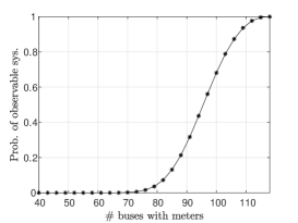
Figure 4: The estimated probability of the IEEE 118-bus system to be observable versus the number of measured buses.

VI-A State estimation and sampling under the DC-PF model

In the following, we evaluate the performance of the GSP-WLS estimator from (33) and compare it with the performance of the pm-WLS estimator from (38). The pm-WLS estimator was generated as follows: First, the a-priori estimated states, $\hat{{\mbox{\boldmath$\theta$}}}_{prior}$, were generated from a zero-mean Gaussian distribution with covariance $0.015{\bf{I}}$. Second, for each simulation we implement the estimator in (38)-(40) by using the random value of $\hat{{\mbox{\boldmath$\theta$}}}_{prior}$ and the covariance ${\bf{R}}_{prior}^{-1}=0.5{\bf{I}}$.

We compare the estimation performance for the following bus selection policies:

1. Random bus selection policy (rand.) - the measured buses are randomly chosen independently from $\{1,\ldots,N\}$, where for more than $72$ buses only observable systems are taken.

2. Experimentally designed sampling (E-design) [35] - the basic assumption behind this method is that the measured graph signal (here the power signal) is an $R$ bandlimited signal in the graph frequency domain. That is, the GFT of ${\bf{z}}_{\text{bus}}$, as defined in (3), satisfies $(\tilde{z}_{\text{bus}})_{n}=0$, $n=R+1,\ldots,N$, where $R$ is the cutoff frequency. Practically, this method maximizes the smallest singular value of the matrix ${\bf{V}}_{{\mathcal{S}},\{1,\ldots,R\}}$, where we set $R=48$, by trial and error. Since in practice the $R$-low-pass assumption does not hold for the power injection signal (as can be seen in Fig. 3), this commonly-used method that was suggested in [53] for power systems, is expected to yield poor performance.

3. Minimum CRB (Alg. 1) - the proposed bus selection policy from Algorithm 1, which does not necessarily result in an observable system.

In Figs. 5(a) and 5(b) the MSE of the GSP-WLS estimator and of the pm-WLS estimator are presented versus the number of measured buses, $q$, and versus $\frac{1}{\sigma^{2}}$, respectively, with the sampling policies 1)-3). Figure 5(b) is obtained for $q=48$ measured buses, for which the system is unobservable with probability almost 1. It can be seen that the MSE decreases as the number of measured buses increases and as $\sigma^{2}$ decreases. In both figures, the GSP-WLS estimator outperforms the pm-WLS estimator for any tested sampling policy. In Fig. 5(a), it can be seen that for each sampling policy, the MSE of the GSP-WLS and the pm-WLS estimators separate from each other where the system becomes unobservable (i.e. where $q<72$ for the random sampling, $q<76$ for the E-design sampling, and $q<79$ for Algorithm 1). In addition, it can be seen that the proposed sampling policy from Algorithm 1 results in a significantly lower MSE than that obtained for the random and the E-design sampling policies for both estimators. In Fig. 5(b) we can see that for small values of $\sigma^{2}$, the differences in the MSE performance of the two estimators are than those obtained for large values of $\sigma^{2}$. This is because the noise impairs the smoothness of the state signal.

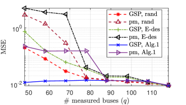
(a)

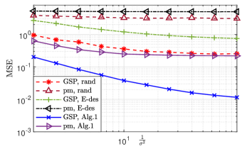
(b)

Figure 5: State estimation under the DC-PF model: The MSE of the GSP-WLS and the pm-WLS estimators for random, E-design, and Algorithm 1 bus selection methods, for the IEEE 118-bus system versus: (a) the number of buses, $q$, with $\sigma^{2}=0.01$; and (b) $\frac{1}{\sigma^{2}}$ with $q=48$ buses.

Figure 6 shows the MSE of the power estimator $\hat{{\bf{z}}}$ from (42) with the three sampling policies. It can be seen that the MSE decreases as the network size increases, as expected, since we have fewer parameters to estimate with the increase in the number of samples (the estimation error in the measured buses is zero) and the state estimation is more accurate, as we presented in Fig. 5(a). In addition, the relations between the sampling policies and the estimation methods are similar to in Fig. 5(a), where the GSP-WLS estimator with the proposed bus selection policy of Algorithm 1 achieves the lowest MSE.

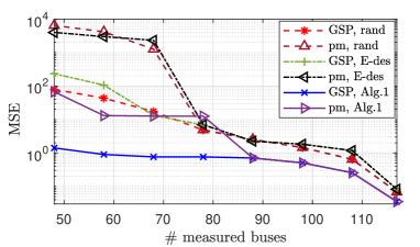
Figure 6: Power estimation based on the DC-PF model: The MSE of the GSP-WLS and the pm-WLS estimators for random, E-design, and Algorithm 1 bus selection methods, for the IEEE 118-bus system and $\sigma^{2}=0.01$ versus the number of buses, $q$.

VI-B State estimation and sampling under the AC-PF model

In the following, we evaluate the performance of the regularized Gauss-Newton method for implementing the GSP-WLS estimator from Algorithm 2, and of the pm-WLS estimator from (2) in the estimation of both the phases and the magnitude. The pm-WLS estimator was also implemented by Algorithm 2 with the appropriate replacements of the regularization terms, i.e. where we use $\hat{{\bf{x}}}_{prior}$ and ${\bf{R}}_{prior}^{-1}={\bf{I}}$ instead of ${\bf{x}}_{0}$ and $\bar{{\bf{L}}}$ (see the discussion after (2)). The maximal number of iterations is set to $l=20$ and $\delta=10^{-8}$.

In Fig. 7 the MSE of phase estimation by the GSP-WLS estimator (implemented by the regularized Gauss-Newton method) and by the pm-WLS estimator are presented versus the number of measured buses, $q$, for the sampling policies 1)-3). Similarly, in Fig. 8 the MSE of the magnitude estimation is presented. It can be seen that the MSE decreases as the number of measured buses increases for both the magnitudes and the phases. It can be seen that the GSP-WLS estimator outperforms the pm-WLS estimator for any sampling policy. In Figs. 7 and 8, it can be seen that for each sampling policy, the MSE of the GSP-WLS and the pm-WLS estimators separate from each other where the system becomes unobservable (i.e. where $q<72$ for the random sampling, $q<76$ for the E-design sampling, and $q<79$ for Algorithm 1). Finally, it can be seen that the sampling policy from Algorithm 1 results in a significantly lower MSE than that obtained for the random and the E-design sampling policies for the GSP-WLS estimator.

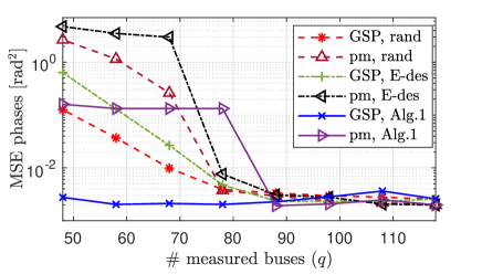
Figure 7: State estimation under the AC-PF model: The phase estimation MSE of the GSP-WLS and the pm-WLS estimators for random, E-design, and Algorithm 1 bus selection methods, for the IEEE 118-bus system versus the number of buses, $q$.

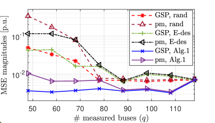
Figure 8: State estimation under the AC-PF model: The magnitude MSE of the GSP-WLS and the pm-WLS estimators for random, E-design, and Algorithm 1 bus selection methods, for the IEEE 118-bus system versus the number of buses, $q$.

VII conclusion

In this paper, we propose a GSP framework for state estimation and sensor placement strategy in unobservable systems. In particular, we first validate the graph smoothness of the phases and the magnitudes of the voltages w.r.t. the admittance matrix. Then, we derive the GSP-WLS estimator for state estimation in unobservable systems under both the DC-PF and AC-PF models. The GSP-WLS estimator uses the graph-smoothness of the state signals as a regularization term. In addition, we introduce a greedy algorithm to tackle the problem of selecting the sampling set that optimizes the state estimation performance. Simulation results demonstrate the potential of the GSP methods in power systems for cases that are otherwise unobservable. It is shown that the proposed methods can accurately estimate voltage phasors (or, equivalently, phases and magnitudes) under low-observability conditions where standard methods cannot. Possible extensions of the proposed GSP framework for power system include the development of approaches based on PMU measurements, the consideration of time-series measurements with temporal dependencies, and the extension to graph neural networks.

References

- [1] A. Abur and A. Gomez-Exposito, Power System State Estimation: Theory and Implementation. Marcel Dekker, 2004.
- [2] T. Routtenberg and L. Tong, “Joint frequency and phasor estimation under the KCL constraint,” IEEE Signal Process. Lett., vol. 20, no. 6, pp. 575–578, June 2013.
- [3] A. Monticelli, State Estimation in Electric Power Systems: A Generalized Approach. Boston, MA: Springer US, 1999, pp. 39–61,91–101,161–199.
- [4] O. Kosut, L. Jia, R. J. Thomas, and L. Tong, “Malicious data attacks on the smart grid,” IEEE Trans. Smart Grid, vol. 2, no. 4, pp. 645–658, Dec. 2011.
- [5] E. Drayer and T. Routtenberg, “Detection of false data injection attacks in smart grids based on graph signal processing,” IEEE Syst. J., vol. 14, no. 2, pp. 1886–1896, 2020.
- [6] G. Morgenstern and T. Routtenberg, “Structural-constrained methods for the identification of unobservable false data injection attacks in power systems,” 2021. [Online]. Available: https://arxiv.org/pdf/2003.08715.pdf
- [7] S. V. Buldyrev, R. Parshani, G. Paul, H. E. Stanley, and S. Havlin, “Catastrophic cascade of failures in interdependent networks,” Nature, vol. 464, no. 7291, pp. 1025–1028, 2010.
- [8] P. Gao, M. Wang, S. G. Ghiocel, J. H. Chow, B. Fardanesh, and G. Stefopoulos, “Missing data recovery by exploiting low-dimensionality in power system synchrophasor measurements,” IEEE Trans. Power Syst., vol. 31, no. 2, pp. 1006–1013, 2016.
- [9] K. R. Mestav, J. Luengo-Rozas, and L. Tong, “Bayesian state estimation for unobservable distribution systems via deep learning,” IEEE Trans. Power Syst., vol. 34, no. 6, pp. 4910–4920, 2019.
- [10] M. B. Do Coutto Filho and J. C. Stacchini de Souza, “Forecasting-aided state estimation—part i: Panorama,” IEEE Trans. Power Syst., vol. 24, no. 4, pp. 1667–1677, 2009.
- [11] K. A. Clements, “The impact of pseudo-measurements on state estimator accuracy,” in IEEE PES General Meeting, 2011, pp. 1–4.
- [12] J. Zhao, G. Zhang, Z. Y. Dong, and M. La Scala, “Robust forecasting aided power system state estimation considering state correlations,” IEEE Trans. Smart Grid, vol. 9, no. 4, pp. 2658–2666, 2018.
- [13] J. Zhao, A. Gómez-Expósito, M. Netto, L. Mili, A. Abur, V. Terzija, I. Kamwa, B. Pal, A. K. Singh, J. Qi, Z. Huang, and A. P. S. Meliopoulos, “Power system dynamic state estimation: Motivations, definitions, methodologies, and future work,” IEEE Trans. Power Syst., vol. 34, no. 4, pp. 3188–3198, 2019.
- [14] S. Bhela, V. Kekatos, and S. Veeramachaneni, “Enhancing observability in distribution grids using smart meter data,” IEEE Trans. Smart Grid, vol. 9, no. 6, pp. 5953–5961, 2018.
- [15] B. Xu and A. Abur, “Observability analysis and measurement placement for systems with PMUs,” in IEEE PES Power Systems Conference and Exposition, 2004, pp. 943–946 vol.2.
- [16] A. S. Zamzam, Y. Liu, and A. Bernstein, “Model-free state estimation using low-rank canonical polyadic decomposition,” IEEE Control Systems Letters, vol. 5, no. 2, pp. 605–610, 2020.
- [17] K. R. Mestav and L. Tong, “Learning the unobservable: High-resolution state estimation via deep learning,” Allerton Conference on Communication, Control, and Computing, pp. 171–176, Dec. 2019.
- [18] J. Zhang, G. Welch, G. Bishop, and Z. Huang, “Reduced measurement-space dynamic state estimation (remedyse) for power systems,” in IEEE Trondheim PowerTech, 2011, pp. 1–7.
- [19] P. L. Donti, Y. Liu, A. J. Schmitt, A. Bernstein, R. Yang, and Y. Zhang, “Matrix completion for low-observability voltage estimation,” IEEE Trans. Smart Grid, vol. 11, no. 3, pp. 2520–2530, 2020.
- [20] A. S. Zamzam and N. D. Sidiropoulos, “Physics-aware neural networks for distribution system state estimation,” IEEE Trans. Power Syst., vol. 35, no. 6, pp. 4347–4356, 2020.
- [21] M. B. Do Coutto Filho, J. C. S. de Souza, and M. T. Schilling, “Generating high quality pseudo-measurements to keep state estimation capabilities,” in IEEE Lausanne Power Tech, 2007, pp. 1829–1834.
- [22] M. Pourali and A. Mosleh, “A functional sensor placement optimization method for power systems health monitoring,” IEEE Trans. Ind Appl., vol. 49, no. 4, pp. 1711–1719, 2013.
- [23] S. Soltan, D. Mazauric, and G. Zussman, “Analysis of failures in power grids,” IEEE Control Netw. Syst., vol. 4, no. 2, pp. 288–300, 2017.
- [24] D. Deka, S. Backhaus, and M. Chertkov, “Estimating distribution grid topologies: A graphical learning based approach,” in Power Systems Computation Conference (PSCC), 2016, pp. 1–7.
- [25] S. Grotas, Y. Yakoby, I. Gera, and T. Routtenberg, “Power systems topology and state estimation by graph blind source separation,” IEEE Trans. Signal Process., vol. 67, no. 8, pp. 2036–2051, Apr. 2019.
- [26] Y. Weng, R. Negi, and M. D. Ilić, “Graphical model for state estimation in electric power systems,” in IEEE International Conference on Smart Grid Communications (SmartGridComm), 2013, pp. 103–108.
- [27] G. B. Giannakis, V. Kekatos, N. Gatsis, S. J. Kim, H. Zhu, and B. F. Wollenberg, “Monitoring and optimization for power grids: A signal processing perspective,” IEEE Signal Processing Magazine, vol. 30, no. 5, pp. 107–128, Sept. 2013.
- [28] T. Ishizaki, A. Chakrabortty, and J. Imura, “Graph-theoretic analysis of power systems,” Proc. of the IEEE, vol. 106, no. 5, pp. 931–952, 2018.
- [29] L. Guo, C. Zhao, and S. H. Low, “Graph Laplacian spectrum and primary frequency regulation,” IEEE CDC, Dec. 2018.
- [30] K. Dvijotham, P. Van Hentenryck, M. Chertkov, S. Misra, and M. Vuffray, “Graphical models for optimal power flow,” Constraints, vol. 22, no. 1, p. 24–49, Sep. 2016.
- [31] N. Retiére, D. T. Ha, and J. Caputo, “Spectral graph analysis of the geometry of power flows in transmission networks,” IEEE Syst. J., vol. 14, no. 2, pp. 2736–2747, 2020.
- [32] A. Sandryhaila and J. M. F. Moura, “Discrete signal processing on graphs,” IEEE Trans. Signal Processing, vol. 61, no. 7, pp. 1644–1656, Apr. 2013.
- [33] A. Ortega, P. Frossard, J. Kovačević, J. M. F. Moura, and P. Vandergheynst, “Graph signal processing: Overview, challenges, and applications,” Proc. of the IEEE, vol. 106, no. 5, pp. 808–828, May 2018.
- [34] D. I. Shuman, S. K. Narang, P. Frossard, A. Ortega, and P. Vandergheynst, “The emerging field of signal processing on graphs: Extending high-dimensional data analysis to networks and other irregular domains,” IEEE Signal Processing Magazine, vol. 30, no. 3, pp. 83–98, May 2013.
- [35] S. Chen, R. Varma, A. Sandryhaila, and J. Kovačević, “Discrete signal processing on graphs: Sampling theory,” IEEE Trans. Signal Process., vol. 63, no. 24, pp. 6510–6523, Dec. 2015.
- [36] A. G. Marques, S. Segarra, G. Leus, and A. Ribeiro, “Sampling of graph signals with successive local aggregations,” IEEE Trans. Signal Process., vol. 64, no. 7, pp. 1832–1843, Apr. 2016.
- [37] R. Ramakrishna and A. Scaglione, “Grid-graph signal processing (grid-GSP): A graph signal processing framework for the power grid,” IEEE Trans. Signal Processing, vol. 69, pp. 2725–2739, 2021.
- [38] N. Retiére, D. T. Ha, and J.-G. Caputo, “Spectral graph analysis of the geometry of power flows in transmission networks,” IEEE Systems Journal, vol. 14, no. 2, pp. 2736–2747, 2020.
- [39] R. Ramakrishna, H. T. Wai, and A. Scaglione, “A user guide to low-pass graph signal processing and its applications: Tools and applications,” IEEE Signal Processing Magazine, vol. 37, no. 6, pp. 74–85, 2020.
- [40] M. Newman, Networks: An Introduction. New York, NY, USA: Oxford University Press, Inc., 2010.
- [41] A. Kroizer, Y. C. Eldar, and T. Routtenberg, “Modeling and recovery of graph signals and difference-based signals,” in IEEE Global Conference on Signal and Information Processing (GlobalSIP), 2019, pp. 1–5.
- [42] M. Aien, M. Fotuhi-Firuzabad, and F. Aminifar, “Probabilistic load flow in correlated uncertain environment using unscented transformation,” IEEE Trans. Power Syst., vol. 27, no. 4, pp. 2233–2241, 2012.
- [43] Y. Chakhchoukh, P. Panciatici, and L. Mili, “Electric load forecasting based on statistical robust methods,” IEEE Trans. Power Syst., vol. 26, no. 3, pp. 982–991, 2011.
- [44] “Power systems test case archive.” [Online]. Available: http://www.ee.washington.edu/research/pstca/
- [45] G. Puy and P. Pérez, “Structured sampling and fast reconstruction of smooth graph signals,” Information and Inference: A Journal of the IMA, vol. 26, pp. 1770–1785, Apr. 2017.
- [46] J. Pang and G. Cheung, “Graph Laplacian regularization for image denoising: Analysis in the continuous domain,” IEEE Trans. Image Process, vol. 7, pp. 657––688, Dec. 2018.
- [47] V. Kalofolias, “How to learn a graph from smooth signals,” Proc. of the conf. on Artifcial Intelligence and Statistics, pp. 920–929, 2016.
- [48] S. Boyd and L. Vandenberghe, Convex Optimization. New York, NY, USA: Cambridge University Press, 2004.
- [49] W. N. van Wieringen, “Lecture notes on ridge regression,” 2020. [Online]. Available: https://arxiv.org/pdf/1509.09169.pdf
- [50] B. Donmez and A. Abur, “Sparse estimation based external system line outage detection,” in Power Systems Computation Conference (PSCC), 2016, pp. 1–6.
- [51] Y. Zhao, J. Chen, A. Goldsmith, and H. V. Poor, “Identification of outages in power systems with uncertain states and optimal sensor locations,” IEEE J. Sel. Topics Signal Process., vol. 8, no. 6, pp. 1140–1153, 2014.
- [52] S. M. Kay, Fundamentals of statistical signal processing: Estimation Theory. Englewood Cliffs (N.J.): Prentice Hall PTR, 1993, vol. 1.
- [53] P. M. Djuric and C. Richard, Cooperative and Graph Signal Processing: Principles and Applications. Academic Press, 2018, ch. 9.