A Nearly Optimal All-Pairs Min-Cuts Algorithm in Simple Graphs

Abstract

We give an $n^{2+o(1)}$-time algorithm for finding $s$-$t$ min-cuts for all pairs of vertices $s$ and $t$ in a simple, undirected graph on $n$ vertices. We do so by constructing a Gomory-Hu tree (or cut equivalent tree) in the same running time, thereby improving on the recent bound of $\tilde{O}(n^{2.5})$ by Abboud et al. (STOC 2021). Our running time is nearly optimal as a function of $n$.

1 Introduction

An $s$-$t$ mincut is a minimum (weight/cardinality) set of edges in a graph whose removal disconnects two vertices $s,t$. Finding $s$-$t$ mincuts, and by duality the value of $s$-$t$ maxflows, is a foundational question in graph algorithms. Naïvely, mincuts for all vertex pairs can be computed by running a maxflow algorithm separately for each vertex pair, thereby incurring $\Theta(n^{2})$ maxflow calls on an $n$-vertex graph. In 1961, Gomory and Hu [GH61] gave a remarkable result where they constructed a cut equivalent tree (or Gomory-Hu tree, after its inventors) that captures an $s$-$t$ mincut for every vertex pair $s,t$ using just $n-1$ maxflow calls. By plugging in the current fastest maxflow algorithm [vdBLL⁺21], this gives an $\tilde{O}(mn+n^{5/2})$-time algorithm for the all pairs min-cuts (apmc) problem on an $n$-vertex, $m$-edge graph. Improving on Gomory and Hu’s 60-year old algorithm for the apmc problem on general, weighted graphs remains a major open question in graph algorithms.

For unweighted graphs however, we can do better. The first algorithm to do so was by Bhalgat et al. [BHKP07], who used Steiner mincuts to obtain a running time of $\tilde{O}(mn)$ in unweighted graphs. Karger and Levine [KL15] matched this bound using the same counting technique, but by a different algorithm based on randomized maxflow computations. In simple graphs, both these algorithms obtain a running time of $\tilde{O}(n^{3})$ since $m=O(n^{2})$. The first subcubic (in $n$) running time was recently obtained in a beautiful work by Abboud et al. [AKT21], who achieved a running time of $\tilde{O}(n^{2.5})$ for simple graphs. They write: “Perhaps the most interesting open question is whether $\tilde{O}(m)$ time can be achieved, even in simple graphs and even assuming a linear-time maxflow algorithm.” Interestingly, they also isolate why breaking the $n^{2.5}$ bound is challenging, and say: “…perhaps it will lead to the first conditional lower bound for computing a Gomory-Hu tree.”

In this paper, we give an $n^{2+o(1)}$-time Gomory-Hu tree algorithm in simple graphs, thereby improving on the $\tilde{O}(n^{2.5})$ bound of Abboud et al. Our result is unconditional – specifically, we do not need to assume an $\tilde{O}(m)$-time maxflow algorithm. As a consequence, we also refute the possibility of a $n^{2.5}$ lower bound for the Gomory-Hu tree problem. Since there are ${n\choose 2}=\Theta(n^{2})$ vertex pairs, the running time of our algorithm is near-optimal for the all-pair mincuts problem. Even if one were to only construct a Gomory-Hu tree (and not report the mincut values explicitly for all vertex pairs), our algorithm is near-optimal as a function of $n$ since $m$ can be $\Theta(n^{2})$.

Our main theorem is the following:

Theorem 1.1.

There is an algorithm $\textsc{GHtree}(G)$ that, given a simple $n$-vertex $m$-edge graph $G$, with high probability computes a Gomory-Hu tree of $G$ in $n^{2+o(1)}$ time.

Our techniques also yield a faster Gomory-Hu tree algorithm in sparse graphs. The previous record for sparse graphs is due to another recent algorithm of Abboud et al. [AKT20b] that takes $O(mc+\sum_{i=1}^{m/c}T(m,n,F_{i}))$ time, where $\sum_{i}F_{i}=O(m)$ and $T(m,n,F_{i})$ is the time complexity for computing a maxflow of value at most $F_{i}$. (Here, $c$ is a parameter that can be chosen by the algorithm designer to optimize the bound.) We improve this bound in the following theorem to $\tilde{O}(mc)+\frac{n^{1+o(1)}}{c}\cdot T(m,n)$ where $T(m,n)$ is the time complexity for computing a maxflow. For comparison, if we assume an $\tilde{O}(m)$-time maxflow algorithm, then the running time improves from $\tilde{O}(m^{1.5})$ in [AKT20b] to $mn^{0.5+o(1)}$ in this paper. Using existing maxflow algorithms [KLS20, vdBLL⁺21], the bound is $\tilde{O}(m\cdot g(m,n))$ in [AKT20b] where $g(m,n)=\min(m^{1/2}n^{1/6},m^{1/2}+n^{3/4})$, and improves to $\sqrt{mn}\cdot n^{o(1)}\cdot g(m,n)$ in this paper.

Theorem 1.2.

There is an algorithm $\textsc{GHtreeSparse}(G)$ that, given a simple $n$-vertex $m$-edge graph $G$, with high probability computes a Gomory-Hu tree of $G$ in $\tilde{O}(mc)+\frac{n^{1+o(1)}}{c}\cdot T(m,n))$ time where $T(m,n)$ denotes the time complexity for computing a maximum flow on an $n$-vertex $m$-edge graph and $c$ is a parameter that we can choose.

Before closing this section, we mention some other results on Gomory-Hu trees, and consequently for the apmc problem. Gusfield [Gus90] gave an algorithm that simplifies Gomory and Hu’s algorithm, particularly from an implementation perspective, although it did not achieve an asymptotic improvement in the running time. If one allows a $(1+\epsilon)$ approximation, then faster algorithms are known; in fact, the problem can be solved using (effectively) $\mathrm{polylog}(n)$ maxflow calls [AKT20a, LP21]. Finally, there is a robust literature on Gomory-Hu tree algorithms for special graph classes. This includes near-linear time algorithms for the class of planar graphs [BSW10] and more generally, for surface-embedded graphs [BENW16], as well as improved runtimes for graphs with bounded treewidth [ACZ98, AKT20a]. For more discussion on the problem, the reader is referred to a survey in the Encyclopedia of Algorithms [Pan16].

Organization.

In Section 2, we introduce the tools that we need for our Gomory-Hu tree algorithm. We then give the Gomory-Hu tree algorithm using these tools, and prove Theorem 1.1 and Theorem 1.2. In subsequent sections, we show how to implement each individual tool and establish their respective properties.

2 Gomory-Hu Tree Algorithm

We start this section by defining Gomory-Hu trees. It will be convenient to also define partial Gomory-Hu trees which will play an important role in our algorithm.

Definition 2.1 (Partial Gomory-Hu trees).

Let $G=(V,E)$ be a graph. A partial Gomory-Hu tree or simply a partial tree $(T,\mathcal{P})$ of $G$ satisfies the following:

• $T$ is a tree on $V(T)\subseteq V$ called a terminal set,

• $\mathcal{P}$ is a partition of $V$ where each part $V_{u}\in\mathcal{P}$ contains exactly one terminal $u$,

• for any pair of terminals $u,v\in V(T)$, a $u$-$v$ mincut $(A_{T},B_{T})$ in $T$ corresponds to a $u$-$v$ mincut $(A,B)$ in $G$ where $A=\bigcup_{x\in A_{T}}V_{x}$ and $B=\bigcup_{y\in B_{T}}V_{y}$.

If $V(T)=V$, then $T$ is a Gomory-Hu tree of $G$.

Terminology about Partial Trees.

Let $X\subseteq V$ be a vertex set. We say that a partial tree $(T,\mathcal{P})$ captures all mincuts separating $X$ of size at most $d$ if, for every part $U\in\mathcal{P}$ and every pair of vertices $u,v\in U\cap X$, $\mathrm{mincut}_{G}(u,v)>d$. When $X=V$, we say that $(T,\mathcal{P})$ captures all mincuts of size at most $d$. If all edges of $T$ have weight at most $d$, then we say that $(T,\mathcal{P})$ captures no mincut of size more than $d$.

We say that $(T^{\prime},\mathcal{P}^{\prime})$ is a refinement of $(T,\mathcal{P})$ if $(T,\mathcal{P})$ can be obtained from $(T^{\prime},\mathcal{P}^{\prime})$ by contracting subtrees of $T^{\prime}$ and taking the union of the corresponding parts of $\mathcal{P}^{\prime}$. In other words, a refinement adds edges while preserving the properties of a partial tree. The classic algorithm of Gomory and Hu [GH61] starts with a vacuous partial tree comprising a single node and refines it in a series of $n-1$ iterations, where each iteration adds a single edge to the tree. Our goal is to refine the partial tree faster by adding multiple edges in a single iteration.

Well-linked Decomposition.

The key to defining a single iteration of our algorithm that refines a partial tree is the notion of a well-linked decomposition. We first define a well-linked set of vertices.

Definition 2.2.

We say that a vertex set $X$ is $(d,\phi)$-well-linked in a graph $G$ if

• For each $v\in X$, $\deg_{G}(v)\geq d$, where $\deg_{G}(v)$ is the degree of vertex $v$ in graph $G$, and

• For each partition $(A,B)$ of $X$, $\frac{\mathrm{mincut}_{G}(A,B)}{d\cdot\min\{|A|,|B|\}}\geq\phi$. Here, $\mathrm{mincut}_{G}(A,B)$ is the smallest cut of $G$ that has vertex subsets $A$ and $B$ on different sides of the cut.

The next lemma is an important technical contribution of our paper, and says that the set of high-degree vertices can be partitioned into a small number of well-linked sets. Actually, this is the only place in this paper where we require that the input graph $G$ is a simple graph.

Lemma 2.3.

There is an algorithm $\textsc{Partition}(G,d)$ that, given a simple $n$-vertex $m$-edge graph $G$ and a parameter $d$, returns with high probability a partition $\{X_{1},\dots,X_{k}\}$ of $V_{\geq d}=\{v\mid\deg_{G}(v)\geq d\}$ such that $k=\tilde{O}(n/d)$ and every set $X_{i}$ is $(d,\phi_{\mathrm{part}})$-well-linked in $G$, where $\phi_{\mathrm{part}}=n^{-o(1)}$. The algorithm $\textsc{Partition}(G,d)$ runs in $m^{1+o(1)}$ time.

In a single iteration, our goal is to refine a partial tree that captures mincuts of size at most $d$ to one that captures mincuts of size at most $2d$. For this, we would like to partition all the vertices in $V_{\geq d}$ using the above lemma, and repeatedly refine the partial tree so that it captures all mincuts of size at most $2d$ separating the terminal set that includes the vertices in the $(d,\phi)$-well-linked set $X_{i}$. But, doing this on the input graph $G$ would be too slow; instead, we use a sparse connectivity certificate that preserves all cuts of size at most $3d$. This suffices since in this iteration, we only seek to capture cuts of size at most $2d$.

Connectivity Certificate.

We formally define connectivity certificates next.

Definition 2.4.

For any graph $G=(V,E)$, a $k$-connectivity certificate $H$ of $G$ is a subgraph of $G$ that preserves all cuts in $G$ of size $<k$, and ensures that all cuts in $G$ of size $\geq k$ have size $\geq k$ in $H$ as well. In other words, for any cut $(S,V\setminus S)$, we have $|E_{H}(S,V\setminus S)|\geq\min\{|E_{G}(S,V\setminus S)|,k\}$.

The next lemma, due to Nagamochi and Ibaraki [NI92], gives an efficient algorithm for obtaining a connectivity certificate.

Lemma 2.5 ([NI92]).

There is an algorithm $\textsc{Sparsify}(G,k)$ that, given an $n$-vertex $m$-edge graph $G$ and a parameter $k$, return a $k$-connectivity certificate $H$ of $G$ with at most $\min\{m,nk\}$ edges in $O(m)$ time.

The Main Lemma.

We are now ready to state our main lemma, which constitutes a refinement of the partial tree.

Lemma 2.6.

There is an algorithm $\textsc{Refine}(G,H,(T,\mathcal{P}),X,d,\phi)$ that given

• graph $G$ on $n$ vertices and $m$ edges, and a $3d$-connectivity certificate $H$ of $G$ with $m^{\prime}\leq\min\{m,3nd\}$ edges,

• a partial tree $(T,\mathcal{P})$ of $G$ that captures all mincuts of size at most $d$ and no mincut of size more than $2d$, and

• a set $X$ that is $(d,\phi)$-well-linked in $H$,

in $\tilde{O}(\min\{m,nd\}/\phi)$ time plus max-flow calls on several graph instances with $\tilde{O}(n/\phi)$ vertices and $\tilde{O}(\min\{m,nd\}/\phi)$ edges in total, returns with high probability a partial tree $(T^{\prime},\mathcal{P}^{\prime})$ of $G$ where

• $(T^{\prime},\mathcal{P}^{\prime})$ is a refinement of $(T,\mathcal{P})$, and

• $(T^{\prime},\mathcal{P}^{\prime})$ captures all mincuts separating $X\cup V(T)$ of size at most $2d$ and no mincut of size more than $2d$.

Crucially, when $3nd\leq m$, the running time in the above lemma does not depend on $m$, the number of edges in $G$. In other words, the algorithm does not even read in the entire graph $G$, instead operating on the $3d$-connectivity certificate $H$ directly.

Small Connectivities.

Recall that in a single iteration, 2.3 produces $\tilde{O}(n/d)$ sets each of which is $(d,\phi_{\mathrm{part}})$-well-linked, and 2.6 makes max-flow calls on graphs with $\tilde{O}(n/\phi_{\mathrm{part}})$ vertices and $\tilde{O}(nd/\phi_{\mathrm{part}})$ edges in total. The current fastest max flow algorithm gives the following runtime:

Theorem 2.7 ([vdBLL⁺21]).

There is an algorithm that can find, with high probability, a maximum flow on a graph with $n$ vertices and $m$ edges in $\tilde{O}(m+n^{1.5})$ time.

Using this algorithm, the runtime of the max flow calls in an iteration becomes $\tilde{O}(\frac{n}{d})\cdot\tilde{O}(nd+n^{1.5})\cdot n^{o(1)}=(n^{2}+\frac{n^{2.5}}{d})\cdot n^{o(1)}$ (recall that $\phi_{\mathrm{part}}=n^{-o(1)}$ in 2.3). While this suffices for $d\geq\sqrt{n}$, we need an additional trick to handle small connectivities, namely $d<\sqrt{n}$.

The next theorem, due to Hariharan et al. [HKP07] and Bhalgat et al. [BHKP07], gives a fast algorithm for computing a partial tree that captures all small cuts:

Theorem 2.8 ([HKP07, BHKP07]).

There is an algorithm $\textsc{SmallConn}(G,d)$ that, given a simple $n$-vertex $m$-edge graph $G$ and a parameter $d$, returns with high probability a partial tree $(T,\mathcal{P})$ that captures all cuts of size at most $d$ in $\tilde{O}(\min\{md,m+nd^{2}\})$ time.

If we set $d=\sqrt{n}$, then this theorem gives a partial tree that captures all cuts of size at most $\sqrt{n}$ in $\tilde{O}(n^{2})$ time. We initialize our algorithm with this partial tree, and then run the iterative refinement process described above for $d=\sqrt{n},2\sqrt{n},\ldots,n/2,n$ to obtain the Gomory-Hu tree. We formally describe this algorithm below and prove its correctness and runtime bounds.

1. Initialize $(T,\mathcal{P})\leftarrow\textsc{SmallConn}(G,c)$ where $c$ is a parameter we can choose.

2. For $d=c,2c,\ldots,n/2,n$

   1. $H\leftarrow\textsc{Sparsify}(G,3d)$

   2. $\{X_{1},\dots,X_{\tilde{O}(n/d)}\}\leftarrow\textsc{Partition}(H,d)$

   3. For each $X_{i}$, $(T,\mathcal{P})\leftarrow\textsc{Refine}(G,H,(T,\mathcal{P}),X_{i},d,\phi_{\mathrm{part}})$

3. Return $T$

Algorithm 1 $\textsc{GHtree}(G)$

The Gomory-Hu Tree Algorithm.

The algorithm is given in Algorithm 1. We first establish correctness of the algorithm. The next property formalizes the progress made by the algorithm in a single iteration of the for loop.

Lemma 2.9.

At the beginning of each for-loop iteration of Algorithm 1, if $(T,\mathcal{P})$ is a partial tree of $G$ that captures all mincuts of size at most $d$ and no mincut of size more than $d$, then at the end of the iteration, $(T,\mathcal{P})$ captures all mincuts of size at most $2d$ and no mincut of size more than $2d$.

Proof.

First, observe that the input to $\textsc{Refine}(\cdot)$ is valid: (1) $H$ is a $3d$-connectivity certificate of $G$ containing $\leq\min\{m,3nd\}$ edges by 2.5, (2) $(T,\mathcal{P})$ is a partial tree of $G$ that captures all mincuts of size at most $d$ and no mincut of size more than $2d$ by assumption, and (3) $X$ is $(d,\phi_{\mathrm{part}})$-well-linked in $H$ by 2.3.

By the second property in 2.6, $(T,\mathcal{P})$ captures no mincut of size more than $2d$. It remains to show that at the end of the iteration, $(T,\mathcal{P})$ captures all mincuts of size at most $2d$. For mincuts of size at most $d$, this follows from the assumption. Consider an $s$-$t$ mincut of size more than $d$ but at most $2d$. Since $s,t\in V_{\geq d}$ in $G$, it follows that $s,t\in V_{\geq d}$ in $H$ as well. Thus, $s,t\in\cup_{i}X_{i}$ produced by $\textsc{Partition}(H,d)$. There are two cases. If $s,t\in X_{i}$ for some $i$, then 2.6 ensures that the $s$-$t$ mincut is captured by $(T,\mathcal{P})$ after $\textsc{Refine}(G,H,(T,\mathcal{P}),X_{i},d,\phi_{\mathrm{part}})$. If $s\in X_{i}$, $t\in X_{j}$ where $i<j$ (wlog), then, when we call $\textsc{Refine}(G,H,(T,\mathcal{P}),X_{j},d,\phi_{\mathrm{part}})$, we have $s\in V(T)$ and $t\in X_{j}$. Again, by 2.6, the $s$-$t$ mincut is captured by $(T,\mathcal{P})$ after the call to Refine. ∎

The following is a simple corollary of the above lemma.

Lemma 2.10.

Algorithm 1 computes a Gomory-Hu tree $T$.

Proof.

First, note that $(T,\mathcal{P})\leftarrow\textsc{SmallConn}(G,c)$ captures all mincuts in $G$ of size at most $c$ by Theorem 2.8. Therefore, by 2.9, at the end of each iteration of the for loop, Algorithm 1 captures all mincuts of size at most $2d$. As a consequence, at the end of the final loop, Algorithm 1 captures all mincuts of size at most $n$. Therefore, $T$ is indeed a Gomory-Hu tree. ∎

We now establish the running time of Algorithm 1.

Lemma 2.11.

By choosing $c=\sqrt{n}$, Algorithm 1 takes $n^{2+o(1)}$ time.

Proof.

$\textsc{SmallConn}(G,c)$ takes $\tilde{O}(m+nc^{2})=\tilde{O}(n^{2})$ time by Theorem 2.8. For each of the $O(\log n)$ iterations, $\textsc{Sparsify}(G,3d)$ takes $O(m)$ time (by 2.5) and $\textsc{Partition}(G,d)$ takes $m^{1+o(1)}=n^{2+o(1)}$ time (by 2.3). Since $H$ has $O(nd)$ edges and $X_{i}$ is $(d,\phi_{\mathrm{part}})$-well-linked, $\textsc{Refine}(G,H,(T,\mathcal{P}),X_{i},d,\phi_{\mathrm{part}})$ takes $(\min\{m,nd\}+n^{1.5})\cdot n^{o(1)}\leq(nd+n^{1.5})\cdot n^{o(1)}$ time by 2.6 and Theorem 2.7. Since there are at most $\tilde{O}(n/d)$ well-linked sets $X_{i}$, the total time spent on Refine is $(n^{2}+n^{2.5}/d)\cdot n^{o(1)}=n^{2+o(1)}$ since $d\geq c=\sqrt{n}$. The lemma follows by summing the time over all iterations. ∎

By analyzing the time differently, we obtain the following.

Lemma 2.12.

For any parameter $c$, Algorithm 1 takes $\tilde{O}(mc)+\frac{n^{1+o(1)}}{c}\cdot T(m,n)$ time where $T(m,n)$ denotes the time complexity for computing a maximum flow on an $n$-vertex $m$-edge graph.

Proof.

$\textsc{SmallConn}(G,c)$ takes $\tilde{O}(mc)$ time. For each of the $O(\log n)$ iterations, $\textsc{Sparsify}(G,3d)$ takes $O(m)$ time (by 2.5) and $\textsc{Partition}(G,d)$ takes $m^{1+o(1)}=m\cdot n^{o(1)}$ time (by 2.3). Also, $\textsc{Refine}(\cdot)$ takes $(\min\{m,nd\}+T(m,n))\cdot n^{o(1)}\leq(m+T(m,n))\cdot n^{o(1)}\leq T(m,n)\cdot n^{o(1)}$ time by 2.6. Since there are at most $\tilde{O}(n/d)=\tilde{O}(n/c)$ well-linked sets $X_{i}$, the total time spent on Refine is $\frac{n^{1+o(1)}}{c}\cdot T(m,n)$. The lemma follows by summing the time over all iterations. ∎

To conclude, observe that Theorem 1.1 follows from 2.10 and 2.11. Similarly, Theorem 1.2 follows from 2.10 and 2.12.

3 Refinement with Well-linked Set

Our goal in this section is to prove the main lemma (2.6). Let us first recall the setting of the lemma. We have a graph $G=(V,E)$ with $n$ vertices and $m$ edges and a $3d$-connectivity certificate $H$ of $G$ containing $m^{\prime}\leq\min\{m,3nd\}$ edges. Let $(T,\mathcal{P})$ be a partial tree of $G$ that captures all mincuts of size at most $d$ and no mincut of size more than $2d$. Let $X$ be a $(d,\phi)$-well-linked set in $H$. For each terminal $u_{i}\in V(T)$ and its corresponding part $V_{i}\in\mathcal{P}$, let $X_{i}=V_{i}\cap X$.

Now, we define the sparsified auxiliary graph $H_{i}$. For each connected component $C$ in $T\setminus\{u_{i}\}$, let $V_{C}=\bigcup_{u\in V(C)}V_{u}$ where each $V_{u}\in\mathcal{P}$. The graph $H_{i}$ is obtained from $H$ by contracting $V_{C}$ into one vertex $u_{C}$ for every component $C$ in $T\setminus\{u_{i}\}$. Let $n^{\prime}_{i}$ and $m^{\prime}_{i}$ denote the number of vertices and edges in $H_{i}$ respectively. ($H_{i}$ is unweighted but not necessarily a simple graph.) Below, we bound the total size of $H_{i}$ over all $i$. The bound on $\sum_{i}m^{\prime}_{i}$ crucially exploits the fact that the graph is unweighted.

Proposition 3.1.

$\sum_{u_{i}\in V(T)}n^{\prime}_{i}\leq 3n$ and $\sum_{u_{i}\in V(T)}m^{\prime}_{i}\leq\min\{3m,5nd\}$.

Proof.

Observe that $n^{\prime}_{i}=|V_{i}|+\deg_{T}(u_{i})$. So $\sum_{u_{i}\in V(T)}n^{\prime}_{i}=n+2|V(T)|\leq 3n$. Next, we bound $\sum_{u_{i}\in V(T)}m^{\prime}_{i}$. For any vertex $x\in V$, let $\mathrm{rep}(x)\in V(T)$ be the unique terminal such that $x\in V_{\mathrm{rep}(x)}$. Consider each edge $(x,y)\in E(H)$. Let $P_{xy}=(\mathrm{rep}(x),\dots,\mathrm{rep}(y))\subseteq V(T)$ be the unique path in $T$ between $\mathrm{rep}(x)$ and $\mathrm{rep}(y)$. (Possibly $x$ and $y$ are in the same part of $\mathcal{P}$ and so $\mathrm{rep}(x)=\mathrm{rep}(y)$.) The crucial observation is that an edge $(x,y)$ appears in $H_{i}$ if and only if the terminal $u_{i}$ is in $P_{xy}$ (otherwise, $x$ are $y$ are contracted into one vertex in $H_{i}$). That is, the contribution of $(x,y)$ to $\sum_{u_{i}\in V(T)}m^{\prime}_{i}$ is exactly $|V_{T}(P_{xy})|=1+|E_{T}(P_{xy})|$. Summing over all edges $e\in E(H)$, this implies that

$$\sum_{u_{i}\in V(T)}m^{\prime}_{i}\leq|E(H)|+\sum_{(x,y)\in E(H)}|E_{T}(P_{xy})|.$$

Recall that $|E(H)|=m^{\prime}\leq\min\{m,3nd\}$. The last important observation is that $\sum_{(x,y)\in E(H)}|E_{T}(P_{xy})|$ is exactly the total weight of edges in $T$. This is because each $(x,y)\in E(H)$ contributes exactly one unit of weight to each tree-edge in $E_{T}(P_{xy})$. The total weight of edges in $T$ is at most $\min\{2m,2nd\}$. To see this, observe that it is at most $(|V(T)|-1)\cdot 2d\leq 2nd$, because $T$ has no edge with weight more than $2d$. Also, it is at most $\sum_{u_{i}\in V(T)}\deg_{G}(u_{i})\leq 2m$ because each tree edge $(u_{i},u_{j})\in E(T)$ has weight $\mathrm{mincut}_{G}(u_{i},u_{j})\leq\min\{\deg_{G}(u_{i}),\deg_{G}(u_{j})\}$. This implies the bound $\sum_{u_{i}\in V(T)}m^{\prime}_{i}\leq\min\{3m,5nd\}$ as claimed. ∎

The key step for proving 2.6 is captured by the following lemma.

Lemma 3.2.

Given $H_{i}$, $X_{i}$, and $(T,\mathcal{P})$, there is an algorithm that takes $\tilde{O}(m^{\prime}_{i}/\phi)$ time and additionally makes max-flow calls on several graphs with $\tilde{O}(n^{\prime}_{i}/\phi)$ vertices and $\tilde{O}(m^{\prime}_{i}/\phi)$ edges in total, and then returns a partial tree $(T^{\prime}_{i},\mathcal{P}^{\prime}_{i})$ of $\boldsymbol{G}$ such that

• $(T^{\prime}_{i},\mathcal{P}^{\prime}_{i})$ is a refinement of $(T,\mathcal{P})$, and

• $(T^{\prime}_{i},\mathcal{P}^{\prime}_{i})$ captures all mincuts separating $X_{i}\cup V(T)$ of size at most $2d$ and no mincut of size more than $2d$.

Before proving 3.2, we show that it implies 2.6. (See Figure 1 for illustration.)

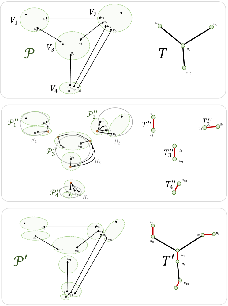
Figure 1: Refining $(T,\mathcal{P})$ to $(T^{\prime},\mathcal{P}^{\prime})$. The algorithm for 3.2 computes partial trees $(T^{\prime\prime}_{i},\mathcal{P}^{\prime\prime}_{i})$ of every sparsified auxiliary graph $H_{i}$. This is illustrated in the second box in the figure above. The algorithm in 3.2 computes a partial tree $(T^{\prime}_{i},\mathcal{P}^{\prime}_{i})$ of $G$ which is a refinement of $(T^{\prime},\mathcal{P})$ in (not shown in the figure above). Then, in the proof of 2.6, we “combine” these refinement on each part $V_{i}$ and we obtain the refined partial tree $(T^{\prime},\mathcal{P}^{\prime})$ of $(T,\mathcal{P})$.

Proof of 2.6.

We apply 3.2 for all $i$ simultaneously and obtain $(T^{\prime}_{i},\mathcal{P}^{\prime}_{i})$ each of which refines $(T,\mathcal{P})$ in exactly one part $V_{i}\in\mathcal{P}$. Let $(T^{\prime},\mathcal{P}^{\prime})$ be the refinement of $(T,\mathcal{P})$ such that $(T^{\prime},\mathcal{P}^{\prime})$ refines the part $V_{i}\in\mathcal{P}$ according to $(T^{\prime}_{i},\mathcal{P}^{\prime}_{i})$ for every $i$. Note that $(T^{\prime},\mathcal{P}^{\prime})$ can be computed in $O(n)$ time. Clearly, $(T^{\prime},\mathcal{P}^{\prime})$ captures no mincut of size more than $2d$ (i.e., $T^{\prime}$ has no edge of weight more than $2d$) because none of $T^{\prime}_{i}$ does.

It remains to prove that $(T^{\prime},\mathcal{P}^{\prime})$ captures all mincuts separating $V(T)\cup\Big{(}\bigcup_{i}X_{i}\Big{)}=V(T)\cup X$ of size at most $2d$. That is, there is no pair $x,y\in V(T)\cup X$ where $\mathrm{mincut}_{G}(x,y)\leq 2d$ and $x,y\in\mathcal{P}^{\prime}$ are in the same part. This is true because, if $x$ and $y$ are from a different part of $\mathcal{P}$, then they are still from a different part in $\mathcal{P}^{\prime}$ as $\mathcal{P}^{\prime}$ is a refinement of $\mathcal{P}$. Otherwise, if $x$ and $y$ are from the same part of $\mathcal{P}$, say $V_{i}\in\mathcal{P}$, then $x,y\in X_{i}\cup V(T)$ and so 3.2 guarantees that they must be separated by $\mathcal{P}^{\prime}_{i}$ and hence in $\mathcal{P}^{\prime}$. This concludes the correctness of 2.6.

Next, we analyze the running time. The total running time is $\sum_{i}\tilde{O}(m^{\prime}_{i}/\phi)=\tilde{O}(\min\{m,nd\}/\phi)$ by 3.1 and 3.2. Finally, the graphs that the algorithm makes max-flow calls on contain in total at most $\sum_{i}\tilde{O}(n^{\prime}_{i}/\phi)=\tilde{O}(n/\phi)$ vertices and $\sum_{i}\tilde{O}(m^{\prime}_{i}/\phi)=\tilde{O}(\min\{m,nd\}/\phi)$ edges by 3.1. This completes the proof.

Proof of 3.2.

For the remaining part of this section, we prove 3.2. There are two main ingredients.

First, we show that the problem of creating a partial tree on a set of terminals can be reduced to finding single source connectivity on the terminals. This step closely mirrors [LP21]: while they focus on the approximate Gomory-Hu tree problem, their techniques translate over to the exact case. Nevertheless, since the reduction might be of independent interest, we give the proof later in Appendix A.

Lemma 3.3.

Let $G=(V,E)$ be an $n$-vertex $m$-edge unweighted (respectively, weighted) graph with a terminal set $X\subseteq V$, and let $k\geq 0$ be a real number. Suppose we have an oracle that, given a terminal $p\in X$, returns $\min\{\mathrm{mincut}_{G}(p,v),k\}$ for all other terminals $v\in X$. Then, there is an algorithm that computes with high probability a partial tree $(T,\mathcal{P})$ of $G$ where $V(T)\subseteq X$ that captures all mincuts separating $X$ of size at most $k$ and no mincuts of size more than $k$. It makes calls to the oracle and max-flow on unweighted (respectively, weighted) graphs with a total of $\tilde{O}(n)$ vertices and $\tilde{O}(m)$ edges, and runs for $\tilde{O}(m)$ time outside of these calls.

Note that it is crucial for us that the reduction above works even when the oracle only returns $\min\{\mathrm{mincut}_{G}(p,v),k\}$ and not $\mathrm{mincut}_{G}(p,v)$. The next lemma exactly implements this oracle:

Lemma 3.4.

Let $G=(V,E)$ be an $n$-vertex $m$-edge graph. Let $X$ be a $(d,\phi)$-well-linked set in $G$. Let $p\in X$ be any fixed vertex in $X$. Then, there is an algorithm that computes $\min\{\mathrm{mincut}_{G}(p,v),2d\}$ for all other $v\in X$ in $O(\frac{m\log n}{\phi})$ time plus $\frac{\mathrm{polylog}(n)}{\phi}$ max-flow calls each on a graph with $O(n)$ vertices and $O(m)$ edges.

We will prove 3.4 in Section 3.1. First, we show how to apply both lemmas above to prove 3.2. We start with a simple observation.

Proposition 3.5.

$X_{i}$ is $(d,\phi)$-well-linked in $H_{i}$.

Proof.

As $X$ is $(d,\phi)$-well-linked in $H$, any subset $X_{i}\subseteq X$ is also $(d,\phi)$-well-linked in $H$. Now, observe that the property that a vertex set is $(d,\phi)$-well-linked is preserved under graph contraction. As $H_{i}$ is a contracted graph of $H$, the proposition follows. ∎

By setting parameters $G\leftarrow H_{i}$ and $X\leftarrow X_{i}$ as the inputs of 3.4, we obtain the required oracle for 3.3 when $k=2d$. By applying 3.3, we obtain a partial tree $(T^{\prime\prime}_{i},\mathcal{P}^{\prime\prime}_{i})$ of $H_{i}$ where $V(T^{\prime\prime}_{i})\subseteq X$, that captures all mincuts separating $X_{i}$ of size at most $2d$ and no mincuts of size more than $2d$. This steps takes $\tilde{O}(m^{\prime}_{i}/\phi)$ time and makes max-flow calls on several graphs with $\tilde{O}(n^{\prime}_{i}/\phi)$ vertices and $\tilde{O}(m^{\prime}_{i}/\phi)$ edges in total.

We are not quite done as we need a partial tree of $G$ (not of $H_{i}$) with all properties required by 3.2, but the remaining steps are quite easy. Suppose the vertex $u_{i}$, which was the unique terminal in $V_{i}$ in the partial tree $(T,\mathcal{P})$, is now in part $V_{u_{i}}\subseteq V(H)$ of the partition $\mathcal{P}^{\prime\prime}_{i}$. Moreover, let $x_{u_{i}}\in X_{i}\cap V(T^{\prime\prime}_{i})$ denote the unique terminal of part $V_{u_{i}}\in\mathcal{P}^{\prime\prime}_{i}$. The algorithm just checks if $\mathrm{mincut}_{H_{i}}(u_{i},x_{u_{i}})\leq 2d$ by using a single max-flow call on $H_{i}$. If so, we further refine $(T^{\prime\prime}_{i},\mathcal{P}^{\prime\prime}_{i})$ according to the mincut separating $u_{i}$ and $x_{u_{i}}$. If not, then we let $u_{i}$ replace $x_{u_{i}}$ as a unique terminal of part $V_{u_{i}}\in\mathcal{P}^{\prime\prime}_{i}$. At this point, $(T^{\prime\prime}_{i},\mathcal{P}^{\prime\prime}_{i})$ is a partial tree of $H_{i}$ that captures all mincuts separating $X_{i}\cup\{u_{i}\}$ of size at most $2d$ and no mincuts of size more than $2d$. Finally, we refine the part $V_{i}$ of $(T,\mathcal{P})$ according to $(T^{\prime\prime}_{i},\mathcal{P}^{\prime\prime}_{i})$ and obtain a partial tree $(T^{\prime}_{i},\mathcal{P}^{\prime}_{i})$ of $G$ as desired. The reason this is correct is because $(T^{\prime\prime}_{i},\mathcal{P}^{\prime\prime}_{i})$ captures only mincuts of size at most $2d$ but $H$ preserves exactly all cuts of $G$ of size at most $3d$. The running times in these final steps are subsumed by the previous steps. This completes the proof of 3.2.

3.1 Single-source Mincut Values for Well-linked Sets: Proof of 3.4

We recall the setting of 3.4. We have an $n$-vertex $m$-edge graph $G$ and a $(d,\phi)$-well-linked set $X$ in $G$. Let $p\in X$ be any fixed vertex in $X$. The goal is to compute $\min\{\mathrm{mincut}_{G}(p,v),2d\}$ for all other $v\in X\setminus\{p\}$.

Now, we need to introduce some notation. We say that a cut $(A,B)$ in $G$ is an $(S,T)$-cut if $S\subseteq A$ and $T\subseteq B$. Moreover, $(A,B)$ is an $(S,T)$-mincut if, additionally, $|E_{G}(A,B)|=\mathrm{mincut}_{G}(S,T)$. We say that $(A,B)$ is the (unique) $S$-minimal $(S,T)$-mincut if, for any $(S,T)$-mincut $(A^{\prime},B^{\prime})$, we have $S\subseteq A\subseteq A^{\prime}$. We will not need the notion of minimal mincut in this section, but it will be used later in Appendix A. A key tool in proving 3.4 is the following Isolating Cuts Lemma of Li and Panigrahi [LP20], which was discovered independently by Abboud, Krauthgamer, and Trabelsi [AKT21].

Lemma 3.6 (Isolating Cut Lemma [LP20, AKT21]).

There is an algorithm that, given an undirected graph $G=(V,E)$ on $n$ vertices and $m$ edges and a terminal set $T\subseteq V$, finds the $t$-minimal $(t,T\setminus\{t\})$-mincut for every $t\in T$ in $O(m\log n)$ time plus $O(\log n)$ maxflow calls each on a graph with $O(n)$ vertices and $O(m)$ edges.

Fix any $x\in X$ where $\mathrm{mincut}_{G}(p,x)\leq 2d$. Let $(A,B)$ be any $(p,x)$-mincut where $p\in A$ and $x\in B$. We have three observations. The first crucial observation says that $(A,B)$ must be “unbalanced” w.r.t. $X$.

Proposition 3.7.

$\min(|A\cap X|,|B\cap X|)\leq\frac{2}{\phi}$.

Proof.

By the well-linkedness of $X$, we have $d\phi\cdot\min(|A\cap X|,|B\cap X|)\leq|E(A,B)|$. On the other hand, we have $|E(A,B)|\leq\mathrm{mincut}_{G}(p,x)\leq 2d$. The bound follows by combining the two inequalities. ∎

Let $S$ be an i.i.d. sample of $X$ with rate $\phi/2$. Let $T=S\cup\{p\}$. The second observation roughly says that, with probability $\Omega(\phi)\geq 1/n^{o(1)}$, one side of $(A,B)$ contains only one vertex from $T$.

Proposition 3.8.

With probability at least $\phi/(2e)$, either

• $A\cap T=\{p\}$ and $x\in T$, or

• $B\cap T=\{x\}$ and $p\in T$.

Proof.

By 3.7, either $|A\cap X|\leq 2/\phi$ or $|B\cap X|\leq 2/\phi$. If $|A\cap X|\leq 2/\phi$, then we have

$$\Pr[A\cap T=\{p\}\text{ and }x\in T]=\Pr[(A\setminus\{p\})\cap S=\emptyset]\cdot\Pr[x\in S]=\left(1-\frac{\phi}{2}\right)^{|A\cap X|-1}\cdot\frac{\phi}{2}\geq\frac{1}{e}\cdot\frac{\phi}{2}$$

If $|B\cap X|\leq 2/\phi$, then we have

$$\Pr[B\cap T=\{x\}\text{ and }p\in T]=\Pr[(B\setminus\{x\})\cap S=\emptyset]\cdot\Pr[x\in S]=\left(1-\frac{\phi}{2}\right)^{|B\cap X|-1}\cdot\frac{\phi}{2}\geq\frac{1}{e}\cdot\frac{\phi}{2}.$$

∎

The last observation says that given that the event in 3.8 happens, then either the $(p,T\setminus\{p\})$-mincut or the $(x,T\setminus\{x\})$-mincut is a $(p,x)$-mincut. This will be useful for us because the Isolating Cut Lemma can compute the $(p,T\setminus\{p\})$-mincut and the $(x,T\setminus\{x\})$-mincut quickly.

Proposition 3.9.

We have the following:

1. If $A\cap T=\{p\}$ and $x\in T$, then any $(p,T\setminus\{p\})$-mincut is a $(p,x)$-mincut.

2. If $B\cap T=\{x\}$ and $p\in T$, then any $(x,T\setminus\{x\})$-mincut is a $(p,x)$-mincut.

Proof.

(1): As $A\cap T=\{p\}$, $(A,B)$ is a $(p,T\setminus\{p\})$-cut and so $\mathrm{mincut}(p,T\setminus\{p\})\leq|E(A,B)|=\mathrm{mincut}(p,x)$. Since $x\in T$, any $(p,T\setminus\{p\})$-cut is a $(p,x)$-cut. Therefore, a $(p,T\setminus\{p\})$-mincut is a $(p,x)$-cut of size at most $\mathrm{mincut}(p,x)$. So it is a $(p,x)$-mincut.

(2): The proof is symmetric. As $B\cap T=\{x\}$, $(B,A)$ is a $(x,T\setminus\{x\})$-cut and so $\mathrm{mincut}(x,T\setminus\{x\})\leq|E(A,B)|=\mathrm{mincut}(p,x)$. Since $p\in T$, any $(x,T\setminus\{x\})$-cut is a $(p,x)$-cut. Therefore, a $(x,T\setminus\{x\})$-mincut is a $(p,x)$-cut of size at most $\mathrm{mincut}(p,x)$. So it is a $(p,x)$-mincut. ∎

1. Initialize $\mathtt{val}[x]=2d$ for all $x\in X\setminus\{p\}$.

2. Repeat $c\cdot\frac{\ln n}{\phi}$ times (for a large enough constant $c$)

   1. Sample $S$ from $X$ i.i.d. at rate $\frac{\phi}{2}$.

   2. Call the Isolating Cuts Lemma (3.6) on terminal set $T=S\cup\{p\}$ and obtain a $(t,T\setminus\{t\})$-mincut $C_{t}$ of size $\delta(C_{t})$ for every $t\in T$.

   3. For each $x\in S\setminus\{p\}$, do the following:

      1. If $C_{x}$ is a $(p,x)$-cut (i.e., $p\notin C_{x}$), then $\mathtt{val}[x]\leftarrow\min\{\mathtt{val}[x],\delta(C_{x})\}$.

      2. If $C_{p}$ is a $(p,x)$-cut (i.e., $x\notin C_{p}$), then $\mathtt{val}[x]\leftarrow\min\{\mathtt{val}[x],\delta(C_{p})\}$.

3. Return $\mathtt{val}[\cdot]$.

Algorithm 2 $\textsc{SingleSourceMincut}(G,X,d,\phi,p)$

The above observations directly suggest an algorithm stated in Algorithm 2. Below, we prove its correctness in 3.10 and bound the running time in 3.11.

Lemma 3.10.

Algorithm 2 computes, with high probability, $\mathtt{val}[x]=\min\{2d,\mathrm{mincut}(p,x)\}$ for all $x\in X\setminus\{p\}$.

Proof.

Note that $\mathtt{val}[x]\leq 2d$ from initialization. So we only need to show that if $\mathrm{mincut}(p,x)\leq 2d$, then $\mathtt{val}[x]=\mathrm{mincut}(p,x)$ whp. On one hand, $\mathtt{val}[x]\geq\mathrm{mincut}(p,x)$ because whenever $\mathtt{val}[x]$ is decreased, it is assigned the size of some $(p,x)$-cut (which is either $C_{x}$ or $C_{p}$). On the other hand, we claim $\mathtt{val}[x]\leq\mathrm{mincut}(p,x)$ whp. To see this, observe that, with probability at least $1-(1-\phi/(2e))^{c\cdot\frac{\ln n}{\phi}}\geq 1-1/n^{10}$, that there exists an iteration in Algorithm 2 where the event in 3.8 happens. That is, $A\cap T=\{p\}$ and $x\in T$, or $B\cap T=\{x\}$ and $p\in T$. Given this, by 3.9, either a $(x,T\setminus\{x\})$-mincut $C_{x}$ or a $(p,T\setminus\{p\})$-mincut $C_{p}$ is a $(p,x)$-mincut and so the algorithm sets $\mathtt{val}[x]\leq\mathrm{mincut}(p,x)$. ∎

Lemma 3.11.

Algorithm 2 takes $O\left(\frac{m\log^{2}n}{\phi}\right)$ time plus $O\left(\frac{\log^{2}n}{\phi}\right)$ max-flow calls each on a graph with $O(n)$ vertices and $O(m)$ edges.

Proof.

Note that $O\left(\frac{\log n}{\phi}\right)$ invocations of 3.6 takes $O\left(\frac{\log^{2}n}{\phi}\right)$ max-flow calls each on a graph with $O(n)$ vertices and $O(m)$ edges plus $O\left(\frac{m\log^{2}n}{\phi}\right)$ time. Additionally, for each invocation of 3.6, we update $\mathtt{val}[\cdot]$ in $O(n)$ time for a total of $O\left(\frac{n\log n}{\phi}\right)$ time. ∎

By 3.10 and 3.11, this completes the proof of 3.4.

4 Well-linked Partitioning

The goal of this section is to prove 2.3. We start with some notation. For disjoint vertex subsets $V_{1},\ldots,V_{\ell}\subseteq V$, define $E_{G}(V_{1},\ldots,V_{\ell})$ as the set of edges $(u,v)\in E$ with $u\in V_{i}$ and $v\in V_{j}$ for some $i\neq j$. For a vector $\mathbf{d}\in\mathbb{R}^{V}$ of entries on the vertices, define $\mathbf{d}(v)$ as the entry of $v$ in $\mathbf{d}$, and for a subset $U\subseteq V$, define $\mathbf{d}(U):=\sum_{v\in U}\mathbf{d}(v)$. We now introduce the concept of an expander “weighted” by demands on the vertices.

Definition 4.1 ($(\phi,\mathbf{d})$-expander).

Consider a weighted, undirected graph $G=(V,E)$ with edge weights $w$ and a vector $\mathbf{d}\in\mathbb{R}^{V}_{\geq 0}$ of non-negative “demands” on the vertices. The graph $G$ is a $(\phi,\mathbf{d})$-expander if for all subsets $S\subseteq V$,

$$\frac{|E_{G}(S,V\setminus S)|}{\min\{\mathbf{d}(S),\mathbf{d}(V\setminus S)\}}\geq\phi.$$

We now state the algorithm of [LS21] that computes our desired expander decomposition, which generalizes the result from [CGL⁺20].

Theorem 4.2 ($(\phi,\mathbf{d})$-expander decomposition algorithm [LS21]).

Fix any $\epsilon>0$ and any parameter $\phi>0$. Given a weighted, undirected graph $G=(V,E)$ with edge weights $w$ and a non-negative demand vector $\mathbf{d}\in\mathbb{R}^{V}_{\geq 0}$ on the vertices, there is a deterministic algorithm running in $m^{1+\epsilon}(\lg n)^{O(1/\epsilon^{2})}$ time that partitions $V$ into subsets $V_{1},\ldots,V_{\ell}$ such that

1. For each $i\in[\ell]$, define the demands $\mathbf{d}_{i}\in\mathbb{R}^{V_{i}}_{\geq 0}$ as $\mathbf{d}$ restricted to the vertices in $V_{i}$. Then, the graph $G[V_{i}]$ is a $(\phi,\mathbf{d}_{i})$-expander.

2. The total number $|E_{G}(V_{1},\ldots,V_{\ell})|$ of inter-cluster edges is $B\phi\cdot\mathbf{d}(V)$ where $B=(\lg n)^{O(1/\epsilon^{4})}$.

Given Theorem 4.2, we can apply it to obtain the desired well-linked sets using the following key lemma:

Lemma 4.3.

There is an algorithm that, given any subset $U\subseteq V_{\geq d}=\{v\mid\deg_{G}(v)\geq d\}$, outputs disjoint subsets $X_{1},\ldots,X_{k}$ of $U$ such that $k\leq 2n/d$, every set $X_{i}$ is $(d,\phi)$-well-linked in $G$ for $\phi=n^{-o(1)}$, and $|\cup_{i}X_{i}|\geq|U|/2$. This algorithm runs in $m^{1+o(1)}$ time.

Proof.

Apply Theorem 4.2 with $\phi=\frac{1}{8B}$ (recall that $B=(\lg n)^{O(1/\epsilon^{4})}$), and the following demands: $\mathbf{d}(v)=d$ for all $v\in U$ and $\mathbf{d}(v)=0$ for all $v\notin U$. (We will set the value of $\epsilon$ later.) We obtain a partition $V_{1},\ldots,V_{\ell}$ of $V$ with $|E_{G}(V_{1},\ldots,V_{\ell})|\leq B\phi\cdot\mathbf{d}(V)=\mathbf{d}(V)/8=d\cdot|U|/8$. For each $i\in[\ell]$ and vertex $v\in U\cap V_{i}$, assign $v$ the value $x(v)=\frac{|E_{G}(V_{i},V\setminus V_{i})|}{|U\cap V_{i}|}$, so that $\sum_{v\in U}x(v)=2|E_{G}(V_{1},\ldots,V_{\ell})|\leq d\cdot|U|/4$. If we select a vertex $v\in U$ uniformly at random, then the expected value of $x(v)$ is at most $d/4$; so, by Markov’s inequality, we have $x(v)\leq d/2$ with probability at least $1/2$. Let $U^{\prime}\subseteq U$ be all vertices $v\in U$ with $x(v)\leq d/2$; it follows that $|U^{\prime}|\geq|U|/2$. For each subset $V_{i}$, the value of $x(v)$ is identical for all vertices in $U\cap V_{i}$. Hence, either $U\cap V_{i}$ is contained in $U^{\prime}$ or is disjoint from it; without loss of generality, let $V_{1},\ldots,V_{k}$ be the sets that are contained in $U^{\prime}$ for some $k\leq\ell$. We now set $X_{i}=U\cap V_{i}$ for all $i\in[k]$.

We first show that each set $X_{i}$ is $(d,\phi)$-well-linked. Since $X_{i}\subseteq U\subseteq V_{\geq d}$, we have $\deg_{G}(v)\geq d$ for all $v\in X_{i}$. Now consider a partition $(A,B)$ of $X_{i}$. For any subset $S\subseteq V_{i}$ that contains $A$ and is disjoint from $B$, we have $|E_{G}(S,V_{i}\setminus S)|\geq\phi\cdot\min\{\mathbf{d}(S),\mathbf{d}(V\setminus S)\}=d\phi\cdot\min\{|A|,|B|\}$, where the inequality holds by definition of $(\phi,\mathbf{d})$-expander. It follows that $\text{mincut}_{G}(A,B)\geq d\phi\cdot\min\{|A|,|B|\}$, and hence, $X_{i}$ is $(d,\phi)$-well-linked.

We now show that $|V_{i}|\geq d/2$ for all $i\in[k]$; since the $V_{i}$ are disjoint, this would imply that $k\leq 2n/d$. Recall that $X_{i}=U\cap V_{i}$, so that $|E_{G}(V_{i},V\setminus V_{i})|=\sum_{v\in X_{i}}x(v)\leq|X_{i}|\cdot d/2$. By averaging, there exists $v\in X_{i}$ with $|E_{G}(v,V\setminus V_{i})|\leq d/2$. Since $\deg_{G}(v)\geq d$, at least $d/2$ edges incident to $v$ must have their other endpoint inside $V_{i}$. Since $G$ is simple, the endpoints must be distinct, so $|V_{i}|\geq d/2$, as promised.

Finally, we fix the value of $\epsilon=(\lg n)^{-1/5}$. Then,

$$\phi=\frac{1}{8B}=\frac{1}{8(\lg n)^{O(1/\epsilon^{4})}}=\frac{1}{8(\lg n)^{O((\lg n)^{4/5})}}=\frac{1}{n^{o(1)}}.$$

The running time is $m^{1+\epsilon}\cdot(\lg n)^{O(1/\epsilon^{2})}=m^{1+(\lg n)^{-1/5}}\cdot(\lg n)^{O(\lg n)^{2/5}}=m^{1+o(1)}$. ∎

We now prove 2.3 using Lemma 4.3. Begin with $U=V_{\geq d}$ and repeatedly apply Lemma 4.3 to obtain disjoint $X_{1},\ldots,X_{k}\subseteq U$, and then reassign $U$ to be $U\setminus\bigcup_{i\in[k]}X_{i}$ for the next iteration; stop when $|U|=1$. Since the size of $U$ halves at each iteration, the number of iterations is at most $\lceil\log_{2}n\rceil$. We thus obtain $\lceil\log_{2}n\rceil\cdot 2n/d$ sets, each of which is $(d,\phi)$-well-linked in $G$, where $\phi=n^{-o(1)}$.

5 Conclusion

In this paper, we gave an $n^{2+o(1)}$-time algorithm for constructing a Gomory-Hu tree in a simple, undirected graph thereby solving the All Pairs Minimum Cuts problem in the same running time. Generalizing this result to weighted graphs, thereby improving on Gomory and Hu’s 60-year old algorithm that uses $n-1$ maxflow calls would be a breakthrough result. An intermediate goal would be to show this for unweighted multigraphs, i.e., allowing parallel edges but not edge weights. The $\tilde{O}(mn)$-time Gomory-Hu tree algorithms of Bhalgat et al. [BHKP07] and of Karger and Levine [KL15] apply to these graphs, but not to general weighted graphs, suggesting that this intermediate class might be easier for the apmc problem than general weighted graphs. Obtaining subcubic (in $n$) running times for the apmc problem in unweighted (but not necessarily simple) graphs remains an interesting open question.

A different question concerns the optimality of the result presented in this paper. As we discussed, our result is nearly optimal if mincut values have to be explicitly reported for all vertex pairs. Even if that is not required, our algorithm is nearly optimal if the input graph is dense, i.e., if $m=\Theta(n^{2})$. So, that leaves graphs containing $o(n^{2})$ edges under the condition that we do not need explicit reporting of mincut values for all vertex pairs. Ideally, for such graphs, one would like to design a near-linear time algorithm, i.e., a running time of $m^{1+o(1)}$. But, that is not known even for a single $s$-$t$ mincut, i.e. for the maxflow problem. A more immediate goal is to construct a Gomory-Hu tree via a subpolynomial (or polylogarithmic) number of maxflow calls. Indeed, this was recently achieved at the cost of obtaining an approximate Gomory-Hu tree instead of an exact one [LP21]. For the exact problem, the current paper gives a reduction, but to polylogarithmic calls of the single source mincut problem rather than the $s$-$t$ mincut problem. Clearly, the former is a more powerful oracle, and hence the reduction is easier. Improving this reduction to the $s$-$t$ mincut problem, or equivalently removing the approximation in the result of [LP21], remains an interesting open question.

Appendix A Reducing Gomory-Hu Tree to Single-Source Mincut Values

The goal of this section is to prove 3.3. Let us first define the problem that the oracle solves, which we name $k$-bounded single source connectivity, abbreviated as $k$-SSC.

Definition A.1 ($k$-SSC).

For a graph $G=(V,E)$, a terminal set $X$, and a source terminal $s\in X$, the output to $k$-SSC is the values $\min\{\mathrm{mincut}_{G}(s,v),k\}$ for all terminals $v\in X\setminus\{s\}$.

Note that in we showed in Section 3.1 how to solve $k$-SSC fast when $X$ is a well-linked set. Below, we will actually prove something stronger than 3.3 by relaxing the task of the oracle: instead of requiring the oracle to compute $k$-SSC, we only require the following verification problem.

Definition A.2 ($k$-SSC Verification).

The input to $k$-SSC Verification is a graph $G=(V,E)$, a terminal set $X$, a source terminal $s\in X$, and values $\tilde{\lambda}_{v}:v\in X\setminus\{s\}$ such that $\tilde{\lambda}_{v}\geq\min\{\mathrm{mincut}(s,v),k\}$. The task is to determine, for each vertex $v\in X\setminus\{s\}$, whether or not $\tilde{\lambda}_{v}=\min\{\mathrm{mincut}(s,v),k\}$.

Clearly, if the oracle can compute $k$-SSC, then it can easily answer $k$-SSC Verification. By focusing on $k$-SSC Verification instead of the original $k$-SSC, we hope to direct future efforts at tackling the former problem, which appears more tractable and is still powerful enough to solve the partial tree problem.

For the rest of this section, we prove the following lemma, which implies 3.3 as discussed above.

Lemma A.3.

For any vertex set $X\subseteq V$ and value $k\geq 0$, there is a randomized algorithm that outputs a partial tree of $G$ that w.h.p., captures all mincuts separating $X$ of size at most $k$ and no mincuts of size more than $k$. It makes calls to max-flow and $k$-SSC Verification on graphs with a total of $\tilde{O}(n)$ vertices and $\tilde{O}(m)$ edges, and runs for $\tilde{O}(m)$ time outside of these calls.

Remark A.4.

This reduction should be compared with the result by [AKT20a] which reduces computing a partial tree to a similar oracle for single source mincuts. The main difference is that their oracle must be able to list edges crossing $(s,v)$-mincuts for each $v\in X\setminus\{s\}$ but, outside the oracle calls, they do not need to call max-flow. Our oracle is potentially easier to implement: we only need to verify mincut values, but our reduction needs to call max flow. Another difference is that their reduction requires the oracle to run on weighted graphs even if the input graph is unweighted, while our oracle only needs to run on unweighted graphs.

Our reduction also holds for weighted graphs (assuming an oracle for weighted graphs), so for completeness, we include the weighted case even though it is not needed for our main result. The only non-trivial modification is that, in the contracted graphs, we combine parallel edges into a edge with combined weights. We show using a different argument that we can still bound the total number of (combined) edges by $\tilde{O}(m)$ over all recursive instances.

Before we present the proof of Lemma A.3, we state a corollary that can be handy (but we do not need it in this paper). It says, given an algorithm for $k$-SSC Verification, we only need to call it and max flow $\tilde{O}(1)$ times to obtain the whole Gomory-Hu tree.

Corollary A.5.

Given a graph $G$ with $n$ vertices and $m$ edges, there is a randomized algorithm that computes a Gomory-Hu tree of $G$ by making calls to max-flow and $k$-SSC Verification (for several different $k$’s) on graphs with a total of $\tilde{O}(n)$ vertices and $\tilde{O}(m)$ edges, and runs for $\tilde{O}(m)$ time outside of these calls.

The proof of Corollary A.5 is simply by calling Lemma A.3 with $k=2^{i}$ from $i=0$ to $O(\log n)$ to iteratively refine the partial tree until it captures all cut sizes, i.e., it becomes a Gomory-Hu tree. Note that this goes in a very similar way as in the proof of 2.6.

Now, we prove Lemma A.3. Our approach for proving Lemma A.3 is almost identical to the one in [LP21], except we adapt their approximate Gomory-Hu tree algorithm to the exact case with the additional $k$-bounded property in mind. The algorithm is described in Algorithm LABEL:ghtree a few pages down. Before we present Algorithm LABEL:ghtree, we first consider the subprocedure LABEL:step that it uses, which mirrors the procedure CutThresholdStep from [LP21]. Below, for any vertex set $S\subset V$, we define $\partial_{G}S=E_{G}(S,V\setminus S)$.

1. Initialize $R^{0}\leftarrow U$ and $D\leftarrow\emptyset$

2. For all $i$ from $0$ to $\lfloor\lg|U|\rfloor$ do:

   1. Call 3.6 on $T=R^{i}$, obtaining a $v$-minimal $(v,R^{i}\setminus v)$-mincut for each $v\in R^{i}$. Let $S^{i}_{v}$ be the side of the $(v,R^{i}\setminus v)$-mincut containing $v$

   2. Call $k$-SSC Verification on graph $G$, terminal set $X=R^{i}$, source $s$, and values $\tilde{\lambda}_{v}=|\partial S^{i}_{v}|$ for $v\in R^{i}\setminus\{s\}$

   3. Let $D^{i}\subseteq R^{i}$ be the union of $S^{i}_{v}\cap U$ over all $v\in R^{i}\setminus\{s\}$ satisfying $\tilde{\lambda}_{v}=\min\{\mathrm{mincut}(s,v),k\}$ and $|S^{i}_{v}\cap U|\leq|U|/2$

   4. $R^{i+1}\leftarrow$ subsample of $R^{i}$ where each vertex in $R^{i}\setminus\{s\}$ is sampled independently with probability $1/2$, and $s$ is sampled with probability $1$

3. Return the largest set $D^{i}$ and the corresponding sets $S^{i}_{v}$ over all $v\in R^{i}\setminus\{s\}$ satisfying the conditions in line 2c

Algorithm 3 LABEL:step$(G=(V,E),s,U,k)$

Let $D=D^{0}\cup D^{1}\cup\cdots\cup D^{\lfloor\lg|U|\rfloor}$ be the union of the sets $D^{i}$ as defined in Algorithm LABEL:step. Let $D^{*}$ be all vertices $v\in U\setminus\{s\}$ for which there exists an $(s,v)$-mincut of size at most $k$ whose $v$ side has at most $|U|/2$ vertices in $U$. The lemma below is almost identical to Lemma 2.5 in [LP21]; the only difference is that CutThresholdStep in [LP21] focuses on solving what they call the Cut Threshold problem, whereas we tackle the partial Gomory-Hu tree problem directly.

Lemma A.6.

We have $D^{i}\subseteq D^{*}$ for all $i$. Moreover, the largest set $D^{i}$ returned by LABEL:step satisfies $\mathbb{E}[|D^{i}|]\geq\Omega(|D^{*}|/\log|U|)$.

Proof.

We first prove that $D^{i}\subseteq D^{*}$ for all $i$. Each vertex $u\in D^{i}$ belongs to some $S^{i}_{v}$ satisfying $|\partial S^{i}_{v}|=\min\{\mathrm{mincut}(s,v),k\}\leq k$ and $|S^{i}_{v}\cap U|\leq|U|/2$. In particular, $\partial S^{i}_{v}$ is an $(s,u)$-mincut of size at most $k$ whose side $S^{i}_{v}$ containing $u$ has at most $|U|/2$ vertices in $U$, so $u\in D^{*}$.

It remains to prove that $\mathbb{E}[|D^{i}|]\geq\Omega(|D^{*}|/\log|U|)$ for the largest set $D^{i}$. For each vertex $v\in D^{*}$, let $S_{v}$ be the minimal $(v,s)$-mincut, and define $U_{v}=S_{v}\cap U$ and $n_{v}=|U_{v}|$. We say that a vertex $v\in D^{*}$ is active if $v\in R^{i}$ for $i=\lfloor\lg n_{v}\rfloor$. In addition, if $U_{v}\cap R^{i}=\{v\}$, then we say that $v$ hits all of the vertices in $U_{v}$ (including itself); see Figure 2. In particular, in order for $v$ to hit any other vertex, it must be active. For completeness, we say that any vertex in $U\setminus D^{*}$ is not active and does not hit any vertex.

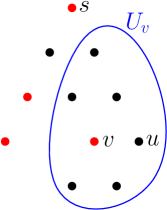
Figure 2: Let $i=\lfloor\lg n_{v}\rfloor=\lfloor\lg 7\rfloor=2$, and let the red vertices be those sampled in $R^{2}$. Vertex $v$ is active and hits $u$ because $v$ is the only vertex in $U_{v}$ that is red.

To prove that $\mathbb{E}[|D^{i}|]\geq\Omega(|D^{*}|/\log|U|)$, we will show that

1. each vertex $u$ that is hit by some vertex $v$ is in $D^{\lfloor\lg n_{v}\rfloor}$,

2. the total number of pairs $(u,v)$ for which $v\in D^{*}$ hits $u$ is at least $c|D^{*}|$ in expectation for some small enough constant $c>0$, and

3. each vertex $u$ is hit by at most $\lfloor\lg|U|\rfloor+1$ vertices.

For (a), let $v$ be the vertex that hits $u$, and consider $i=\lfloor\lg n_{v}\rfloor$. We have $U_{v}\cap R^{i}=\{v\}$ by assumption, so $\partial S_{v}$ is a $(v,R^{i}\setminus\{v\})$-cut. On the other hand, we have that $\partial S^{i}_{v}$ is a $(v,R^{i}\setminus\{v\})$-mincut, so in particular, it is a $(v,s)$-cut. It follows that $\partial S_{v}$ and $\partial S^{i}_{v}$ are both $(v,s)$-mincuts and $(v,R^{i}\setminus v)$-mincuts, and $|\partial S^{i}_{v}|=\mathrm{mincut}(s,v)\leq k$. Since $S_{v}$ is the minimal $(v,s)$-mincut and $S^{i}_{v}$ is a $(v,s)$-mincut, we must have $S_{v}\subseteq S^{i}_{v}$. Likewise, since $S_{v}$ is a $(v,R^{i}\setminus\{v\})$-mincut and $S^{i}_{v}$ is the minimal $(v,R^{i}\setminus\{v\})$-mincut, we also have $S^{i}_{v}\subseteq S_{v}$. It follows that $S_{v}=S^{i}_{v}$. Since $S_{v}$ is the minimal $(v,s)$-mincut and $v\in D^{*}$, we must have $|S_{v}\cap U|\leq z$, so in particular, $|S^{i}_{v}\cap U|=|S_{v}\cap U|\leq z$. Therefore, the vertex $v$ satisfies all the conditions of line 2c. Moreover, since $u\in U_{v}\subseteq S_{v}=S^{i}_{v}$, vertex $u$ is added to $D$ in the set $S^{i}_{v}\cap U$.

For (b), for $i=\lfloor\lg n_{v}\rfloor$, we have $v\in R^{i}$ with probability exactly $1/2^{i}=\Theta(1/n_{v})$, and with probability $\Omega(1)$, no other vertex in $U_{v}$ joins $R^{i}$. Therefore, $v$ is active with probability $\Omega(1/n_{v})$. Conditioned on $v$ being active, it hits exactly $n_{v}$ many vertices. It follows that $v$ hits $\Omega(1)$ vertices in expectation. Summing over all $v\in D^{*}$ and applying linearity of expectation proves (b).

For (c), since the isolating cuts $S^{i}_{v}$ over $v\in R^{i}$ are disjoint for each $i$, each vertex is hit at most once on each iteration $i$. Since there are $\lfloor\lg|U|\rfloor+1$ many iterations, the property follows.

Finally, we show why properties (a) to (c) imply $\mathbb{E}[|D^{i}|]\geq\Omega(|D^{*}|/\log|U|)$ for the largest $D^{i}$. By property (b), the number of times some vertex hits another vertex is $\Omega(|D^{*}|)$ in expectation. Since there are $\lfloor\lg|U|\rfloor+1$ many distinct values of $\lfloor\lg n_{v}\rfloor$, there exists an integer $i$ for which the number of times some vertex $v$ with $\lfloor\lg n_{v}\rfloor=i$ hits another vertex is $\Omega(|D^{*}|/\log|U|)$ in expectation. Since each vertex is hit at most once on iteration $i$, there must be $\Omega(|D^{*}|/\log|U|)$ many vertices hit, all of which are included in $D^{i}$ by property (a). ∎

1. Compute the Steiner connectivity $\lambda\leftarrow\min_{u,v\in U}\mathrm{mincut}_{G}(u,v)$ w.r.t. terminals $U$

2(If $|U|=1$, then $\lambda=\infty$)

$\triangleright$ $\tilde{O}(|E|)$ time plus max-flow calls on graphs totalling $\tilde{O}(|V|)$ vertices and $\tilde{O}(|E|)$ edges [CQ21]

If $\lambda>k$, then terminate and return the trivial partial tree $(T,\mathcal{P})$ with $V(T)=\{v\}$ for an arbitrary $v\in U$ and $\mathcal{P}=\{U\}$ as the trivial partition of $U$ 3. $s\leftarrow$ uniformly random vertex in $U$ 4. Call $\ref{step}(G,s,U,k)$ to obtain $D^{i}$ and the sets $S^{i}_{v}$ (so that $D^{i}=\bigcup_{v}S^{i}_{v}\cap U$)  5. For each set $S^{i}_{v}$ do: $\triangleright$ Construct recursive graphs and apply recursion (a) Let $G_{v}$ be the graph $G$ with vertices $V\setminus S^{i}_{v}$ contracted to a single vertex $x_{v}$ $\triangleright$ $S^{i}_{v}$ are disjoint (b) Let $U_{v}\leftarrow S^{i}_{v}\cap U$ (c) If $|U_{v}|>1$, then recursively set $(T_{v},\mathcal{P}_{v})\leftarrow\ref{ghtree}(G_{v},U_{v})$ 6. Let $G_{\textup{large}}$ be the graph $G$ with (disjoint) vertex sets $S^{i}_{v}$ contracted to single vertices $y_{v}$ for all $v\in D^{i}$ 7. Let $U_{\textup{large}}\leftarrow U\setminus D^{i}$ 8. If $|U_{\textup{large}}|>1$, then recursively set $(T_{\textup{large}},\mathcal{P}_{\textup{large}})\leftarrow\ref{ghtree}(G_{\textup{large}},U_{\textup{large}})$ 9. Combine $(T_{\textup{large}},\mathcal{P}_{\textup{large}})$ and $\{(T_{v},\mathcal{P}_{v}):v\in D^{i}\}$ into $(T,\mathcal{P})$ according to LABEL:combine 10. Return $(T,\mathcal{P})$

Algorithm 4 LABEL:ghtree$(G=(V,E),U,k)$

1

1. Construct $T$ by starting with the disjoint union $T_{\textup{large}}\cup\bigcup_{v\in R^{i}}T_{v}$ and, for each $v\in R^{i}$, adding an edge $(x,y)$ of weight $|\partial_{G}S^{i}_{v}|$, where $x_{v}\in V_{x}$ and $y_{v}\in V_{y}$

2. Construct $\mathcal{P}$ as the disjoint union of partitions $\mathcal{P}_{\textup{large}}$ and $\mathcal{P}_{v}$ over all $v\in R^{i}$, restricted to vertices in $V$

3. Return $(T,\mathcal{P})$

Algorithm 5 LABEL:combine$((T_{\textup{large}},\mathcal{P}_{\textup{large}}),\{(T_{v},\mathcal{P}_{v}):v\in R^{i}\})$

Now, we state Algorithm 4 for Lemma A.3 and prove its correctness below.

Lemma A.7 (Correctness).

For any vertex set $U\subseteq V$ and value $k\geq 0$, the algorithm $\ref{ghtree}(G,U,k)$ returns a partial tree $(T,\mathcal{P})$ in $G$ with the terminal set $V(T)\subseteq U$ that captures all mincuts separating $U$ of size at most $k$ and no mincuts of size more than $k$.

We give a detailed proof of Lemma A.7 in Section A.1 because it follows using a standard argument. Here, we give only a high-level argument: although in each recursion level of Algorithm 4, the algorithm refines the tree into many parts, these refinements can be simulated by a sequence of the standard refinement steps in the original Gomory-Hu tree algorithm that splits only one supernode/part into two. So the resulting $(T,\mathcal{P})$ is indeed a partial tree of $G$. Next, $(T,\mathcal{P})$ captures no mincut of size more than $k$ because all edges in $T$ have weight at most $k$ by construction. It remains to argue why $(T,\mathcal{P})$ captures all mincuts of size at most $k$ separating terminals $U$, let $x,y\in U$ where $\mathrm{mincut}_{G}(x,y)\leq k$. We want to say that $x,y$ are in different parts of $\mathcal{P}$. There are two main cases. If both $x,y\in U_{{\textup{large}}}$ or both $x,y\in U_{v}$ for some $v\in D^{i}$, then, by induction, $x$ are $y$ will be separated in $\mathcal{P}_{{\textup{large}}}$ or in $\mathcal{P}_{v}$ respectively, and they remain separated in $\mathcal{P}$ by how the Combine subroutine works. Otherwise, we have that $x\in U_{v}$ and $y\notin U\setminus U_{v}$, then they are in different subproblems in the recursion and remain separated in $\mathcal{P}$ by how the Combine subroutine works.

The remaining part of this section is for bounding the running time of Algorithm 4. For any $U\subseteq V$, define $f_{k}(U)$ as the size of the largest subset of vertices in $U$ whose pairwise mincut values are all greater than $k$. The following lemma is inspired by [AKT20a]. (In fact, our statement and proof are identical to theirs in the case $k=\infty$.)

Claim A.8.

Let the vertex $s\in U$ be chosen uniformly at random. Then, $\mathbb{E}[|D^{*}|]=(|U|-f_{k}(U))/2$.

Proof.

Consider the partial tree $(T,\mathcal{P})$ that captures all mincuts separating $U$ of size at most $k$ and no mincuts of size more than $k$. In other words, vertices $x,y\in U$ belonging to different parts of $\mathcal{P}$ iff $\mathrm{mincut}(x,y)\leq k$. By the definition of $f_{k}(U)$, the maximum size of a part in $\mathcal{P}$ is $f_{k}(U)$. Consider a digraph on vertex set $U$ where for each pair of vertices $x,y\in U$, we add a directed edge $(x,y)$ if there exists an $(x,y)$-mincut of size at most $k$ where the side containing $x$ has at most $|U|/2$ vertices in $U$. Clearly, for each $x,y\in U$ with $\mathrm{mincut}(x,y)\leq k$, we add either $(x,y)$ or $(y,x)$ (or both) to the digraph. Also, for each vertex $x\in U$, the vertices $y\in U$ with $\mathrm{mincut}(x,y)\leq k$ are exactly those not in the same part as $u$ in $\mathcal{P}$, so there are at least $|U|-f_{k}(U)$ such vertices $y$. Therefore, the total number of arcs entering or leaving $u$ is at least $|U|-f_{k}(U)$. The total number of arcs in the digraph is at least $|U|(|U|-f_{k}(U))/2$, so the average out-degree is at least $(|U|-f_{k}(U))/2$. Note that for the vertex $s$ chosen uniformly at random, the set $|D^{*}|$ is exactly the out-neighbors of $s$. It follows that $\mathbb{E}[|D^{*}|]\geq(|U|-f_{k}(U))/2$. ∎

Lemma A.9.

W.h.p., the algorithm LABEL:ghtree has maximum recursion depth $\mathrm{polylog}(n)$.

Proof.

By construction, each recursive instance $(G_{v},U_{v})$ has $|U_{v}|\leq|U|/2$.

By Lemma A.6 and A.8, over the randomness of $s$ and LABEL:step, we have

$$\mathbb{E}[D^{i}]\geq\Omega\left(\frac{\mathbb{E}[|D^{*}|]}{\log|U|}\right)\geq\Omega\left(\frac{|U|-f_{k}(U))}{\log|U|}\right).$$

If $f_{k}(U)\leq\frac{2}{3}|U|$, then this is $\Omega(|U|/\log|U|)$, so the recursive instance $(G_{\textup{large}},U_{\textup{large}})$ satisfies $\mathbb{E}[|U_{\textup{large}}|]\leq(1-1/\log|U|)\cdot|U|$. Suppose now that $f_{k}(U)\geq\frac{2}{3}|U|$, and let $U^{\prime}\subseteq U$ be the vertex set of size $f_{k}(U)$ whose pairwise mincut values exceed $k$. By construction, the entire set $U^{\prime}$ is contained in either $U_{\textup{large}}$ or $U_{v}$ for some $v\in D^{i}$, and since $|U_{v}|\leq|U|/2$ for all $v\in D^{i}$, we must have $U^{\prime}\subseteq U_{\textup{large}}$. In other words, $f_{k}(U_{\textup{large}})=f_{k}(U)$. So the recursive instance $(G_{\textup{large}},U_{\textup{large}})$ satisfies

$$\mathbb{E}[|U_{\textup{large}}|-f_{k}(U_{\textup{large}})]=\mathbb{E}[|U_{\textup{large}}|]-f_{k}(U) \geq|U|-\Omega\left(\frac{|U|-f_{k}(U)}{\log|U|}\right)-f_{k}(U)$$

$$=\left(1-\Omega\bigg{(}\frac{1}{\log|U|}\bigg{)}\right)(|U|-f_{k}(U)).$$

Therefore, each recursive branch has either $|U|-f_{k}(U)$ dropped by factor $(1-\Omega(1/\log|U|))$ in expectation, or $|U|$ dropped by factor $(1-\Omega(1/\log|U|))$ in expectation (and $|U|-f_{k}(U)$ can potentially increase). It follows that w.h.p., all branches reach $|U|=f_{k}(U)$ or $|U|=1$ by $\mathrm{polylog}(n)$ recursive calls. In both cases, the value $\lambda$ in line 4 has $\lambda>k$, so the algorithm terminates. ∎

Lemma A.10 (Running time).

For an unweighted (respectively, weighted) graph $G=(V,E)$, and terminals $U\subseteq V$, and value $k\geq 0$, $\ref{ghtree}(G,U,k)$ takes time $\tilde{O}(m)$ plus calls to $k$-SSC Verification and max-flow on unweighted (respecively, weighted) instances with a total of $\tilde{O}(n)$ vertices and $\tilde{O}(m)$ edges.

Proof.

For a given recursion level, consider the instances $\{(G_{i},U_{i},k)\}_{i}$ across that level. By construction, the terminals $U_{i}$ partition $U$. Moreover, the total number of vertices over all $G_{i}$ is at most $n+2(|U|-1)=O(n)$ since each branch creates $2$ new vertices and there are at most $|U|-1$ branches.

To bound the total number of edges, we consider the unweighted and weighted cases separately, starting with the unweighted case. The total number of new edges created is at most the sum of weights of the edges in the final Gomory-Hu Steiner tree. For an unweighted graph, this is $O(m)$ by the following well-known argument. Root the Gomory-Hu Steiner tree $T$ at any vertex $r\in U$; for any $v\in U\setminus r$ with parent $u$, the cut $\partial\{v\}$ in $G$ is a $(u,v)$-cut of value $\deg(v)$, so $w_{T}(u,v)\leq\lambda_{G}(u,v)\leq\deg(v)$. Overall, the sum of the edge weights in $T$ is at most $\sum_{v\in U}\deg(v)\leq 2m$.

For the weighted case, define a parent vertex in an instance as a vertex resulting from either (1) contracting $V\setminus S_{v}$ in some previous recursive $G_{v}$ call, or (2) contracting a component containing a parent vertex in some previous recursive call. There are at most $O(\log n)$ parent vertices: at most $O(\log n)$ can be created by (1) since each $G_{v}$ call decreases $|U|$ by a constant factor, and (2) cannot increase the number of parent vertices. Therefore, the total number of edges adjacent to parent vertices is at most $O(\log n)$ times the number of vertices. Since there are $O(n)$ vertices in a given recursion level, the total number of edges adjacent to parent vertices is $O(n\log n)$ in this level. Next, we bound the number of edges not adjacent to a parent vertex by $m$. To do so, we first show that on each instance, the total number of these edges over all recursive calls produced by this instance is at most the total number of such edges in this instance. Let $P\subseteq V$ be the parent vertices; then, each $G_{v}$ call has exactly $|E(G[S_{v}\setminus P])|$ edges not adjacent to parent vertices (in the recursive instance), and the $G_{\textup{large}}$ call has at most $|E(G[V\setminus P])\setminus\bigcup_{v\in R}E(G[S_{v}\setminus P])|$, and these sum to $|E(G[V\setminus P])|$, as promised. This implies that the total number of edges not adjacent to a parent vertex at the next level is at most the total number at the previous level. Since the total number at the first level is $m$, the bound follows.

Therefore, there are $O(n)$ vertices and $\tilde{O}(m)$ edges in each recursion level. By Lemma A.9, there are $\text{polylog}(n)$ levels, for a total of $\tilde{O}(n)$ vertices and $\tilde{O}(m)$ edges. In particular, the instances to the max-flow calls have $\tilde{O}(n)$ vertices and $\tilde{O}(m)$ edges in total. ∎

A.1 Proof of Lemma A.7

To prove Lemma A.7, we first introduce a helper proposition, which follows from the standard argument on non-crossing cuts used in the original Gomory-Hu algorithm. We include the proof only for completeness.

Proposition A.11.

For any distinct vertices $p,q\in U_{\textup{large}}$, we have $\mathrm{mincut}_{G_{\textup{large}}}(p,q)=\mathrm{mincut}_{G}(p,q)$. The same holds with $U_{\textup{large}}$ and $G_{\textup{large}}$ replaced by $U_{v}$ and $G_{v}$ for any $v\in D^{i}$.

Proof.

Since $G_{\textup{large}}$ is a contraction of $G$, we have $\mathrm{mincut}_{G_{\textup{large}}}(p,q)\geq\mathrm{mincut}_{G}(p,q)$. To show the reverse inequality, fix any $(p,q)$-mincut in $G$, and let $S$ be one side of the mincut. We show that for each $v\in D^{i}$, either $S^{i}_{v}\subseteq S$ or $S^{i}_{v}\subseteq V\setminus S$. Assuming this, the cut $\partial_{G}S$ stays intact when the sets $S^{i}_{v}$ are contracted to form $G_{\textup{large}}$, so $\mathrm{mincut}_{G_{\textup{large}}}(p,q)\leq|\partial_{G}S|=\mathrm{mincut}_{G}(p,q)$.

Consider any $v\in D^{i}$, and suppose first that $v\in S$. Then, $S^{i}_{v}\cap S$ is still a $(v,R^{i}\setminus v)$-cut, and $S^{i}_{v}\cup S$ is still a $(p,q)$-cut. By the submodularity of cuts,

$$|\partial_{G}S^{i}_{v}|+|\partial_{G}S|\geq|\partial_{G}(S^{i}_{v}\cup S)|+|\partial_{G}(S^{i}_{v}\cap S)|.$$

In particular, $S^{i}_{v}\cap S$ must be a $(v,R^{i}\setminus v)$-mincut. Since $S^{i}_{v}$ is the $v$-minimal $(v,R^{i}\setminus v)$-mincut by 3.6 called in subprocedure LABEL:step, it follows that $S^{i}_{v}\cap S=S^{i}_{v}$, or equivalently, $S^{i}_{v}\subseteq S$.

Suppose now that $v\notin S$. In this case, we can swap $p$ and $q$, and swap $S$ and $V\setminus S$, and repeat the above argument to get $S^{i}_{v}\subseteq V\setminus S$.

The argument for $U_{v}$ and $G_{v}$ is identical, and we skip the details. ∎

Proof (Lemma A.7)..

By construction, all edges in $T$ have weight at most $k$ (i.e., it captures no mincut of size more than $k$). It remains to show that it captures all mincuts separating $U$ of size at most $k$. That is, for all $x,y\in U$ with $\mathrm{mincut}(x,y)\leq k$, there is an edge on the $x$-$y$ path in $T$ of weight $\mathrm{mincut}(x,y)$.

We apply induction on $|U|$. By induction, the recursive outputs $(T_{\textup{large}},\mathcal{P}_{\textup{large}})$ and $(T_{v},\mathcal{P}_{v})$ are partial trees capturing all mincuts separating $U_{\textup{large}}$ in $G_{\textup{large}}$ and $U_{v}$ in $G_{v}$, respectively, of size at most $k$.

First, consider $x,y\in U_{\textup{large}}$ with $\mathrm{mincut}(x,y)\leq k$, so that the partition $\mathcal{P}_{\textup{large}}$ separates $x$ and $y$. Let $(u,u^{\prime})$ be the minimum-weight edge on the $x$-$y$ path in $T_{\textup{large}}$, and let $U^{\prime}_{\textup{large}}\subseteq U_{\textup{large}}$ be the vertices of the connected component of $T_{\textup{large}}\setminus(u,u^{\prime})$ containing $x$, so that $V_{U^{\prime}_{\textup{large}}}$ is an $(s,t)$-mincut in $G_{\textup{large}}$ with value $w_{T}(u,u^{\prime})$. Define $U^{\prime}\subseteq U$ as the vertices of the connected component of $T\setminus(u,u^{\prime})$ containing $x$. By construction of $(T,\mathcal{P})$, $G_{\textup{large}}$ is simply $G$ with all vertex sets $S^{i}_{v}$ contracted to $y_{v}$ for all $v\in D^{i}$. Similarly, $V_{U^{\prime}_{\textup{large}}}$ (union of parts $V_{z}:z\in U^{\prime}_{\textup{large}}$ from $\mathcal{P}_{\textup{large}}$) is simply the set $V_{U^{\prime}}$ (union of parts $V_{z}:z\in U^{\prime}$ from $\mathcal{P}$) where all vertex sets $S^{i}_{v}$ are contracted to $y_{v}$ for all $v\in D^{i}$. So we conclude that $w_{G_{\textup{large}}}(V_{U^{\prime}_{\textup{large}}})=w_{G}(V_{U^{\prime}})$. By A.11, we have $\mathrm{mincut}_{G}(x,y)=\mathrm{mincut}_{G_{\textup{large}}}(x,y)$ are equal, so $w_{G}(V_{U^{\prime}})$ is an $(x,y)$-mincut in $G$. In other words, the partial tree condition for $(T,\mathcal{P})$ is satisfied for all $x,y\in U_{\textup{large}}$ with $\mathrm{mincut}(x,y)\leq k$. A similar argument handles the case $x,y\in U_{v}$ with $\mathrm{mincut}(x,y)\leq k$ for some $v\in D^{i}$.

Consider now $x,y\in U$ with $\mathrm{mincut}(x,y)\leq k$, and either $x\in U_{v}$ and $y\in U_{\textup{large}}$, or $x\in U_{v}$ and $y\in U_{v^{\prime}}$ for distinct $v,v^{\prime}\in D^{i}$. Suppose first that $x\in U_{v}$ and $y\in U_{\textup{large}}$. By considering which sides $v$ and $s$ lie on the $(x,y)$-mincut $(S,V\setminus S)$, we have

$$|\partial_{G}S|=\mathrm{mincut}(x,y)\geq\min\{\mathrm{mincut}(x,v),\mathrm{mincut}(v,s),\mathrm{mincut}(s,y)\}.$$

We case on which of the three mincut values $\mathrm{mincut}(x,y)$ is greater than or equal to.

1. If $\mathrm{mincut}(x,y)\geq\mathrm{mincut}(v,s)$, then since $S^{i}_{v}$ is a $(v,s)$-mincut that is also an $(x,y)$-cut, we have $\mathrm{mincut}(x,y)=\mathrm{mincut}(v,s)\leq k$. By construction, there is an edge $e$ of weight $|\partial_{G}S^{i}_{v}|=|\partial_{G}S|$ on the $x$-$y$ path in $T$. There cannot be edges on the $x$-$y$ path in $T$ of smaller weight, since each edge corresponds to a $(x,y)$-cut in $G$ of the same weight. Therefore, $e$ is the minimum-weight edge on the $x$-$y$ path in $T$.

2. Suppose now that $\mathrm{mincut}(x,v)\leq\mathrm{mincut}(x,y)<\mathrm{mincut}(v,s)$. Let $z\in U_{v}$ be the vertex with $x_{v}\in V_{z}$ (for partition $\mathcal{P}_{v}$). Since $\mathrm{mincut}(x,v)\leq\mathrm{mincut}(x,y)\leq k$, the vertices $x,v$ are separated by the partition $\mathcal{P}_{v}$, and the minimum-weight edge $e$ on the $x-v$ path in $T_{v}$ has weight $\mathrm{mincut}(x,v)$. This edge $e$ cannot be on the $v-z$ path in $T_{v}$, since otherwise, we would obtain a $(v,x_{v})$-cut of value $\mathrm{mincut}(x,v)$ in $G_{v}$, which becomes a $(v,s)$-cut in $G$ after expanding the contracted vertex $x_{v}$; this contradicts our assumption that $\mathrm{mincut}(x,v)<\mathrm{mincut}(v,s)$. It follows that $e$ is on the $x-z$ path in $T_{v}$ which, by construction, is also on the $x-y$ path in $T$. Once again, the $x-y$ path cannot contain an edge of smaller weight.

3. The final case $\mathrm{mincut}(s,y)\leq\mathrm{mincut}(x,y)<\mathrm{mincut}(v,s)$ is symmetric to case 2, except we argue on $T_{\textup{large}}$ and $G_{\textup{large}}$ instead of $T_{v}$ and $G_{v}$.

Suppose now that $x\in U_{v}$ and $y\in U_{v^{\prime}}$ for distinct $v,v^{\prime}\in D^{i}$. By considering which sides $v,v^{\prime},s$ lie on the $(x,y)$-mincut, we have

$$|\partial_{G}S|=\mathrm{mincut}(x,y)\geq\min\{\mathrm{mincut}(x,v),\mathrm{mincut}(v,s),\mathrm{mincut}(s,v^{\prime}),\mathrm{mincut}(v^{\prime},y)\}.$$

We now case on which of the four mincut values $\mathrm{mincut}(x,y)$ is greater than or equal to.

1. If $\mathrm{mincut}(x,y)\geq\mathrm{mincut}(v,s)$ or $\mathrm{mincut}(x,y)\geq\mathrm{mincut}(s,v^{\prime})$, then the argument is the same as case 1 above.

2. If $\mathrm{mincut}(x,v)\leq\mathrm{mincut}(x,y)<\mathrm{mincut}(v,s)$ or $\mathrm{mincut}(y,v^{\prime})\leq\mathrm{mincut}(x,y)<\mathrm{mincut}(v^{\prime},s)$, then the argument is the same as case 2 above.

This concludes all cases, and hence the proof. ∎

References

- [ACZ98] Srinivasa Rao Arikati, Shiva Chaudhuri, and Christos D. Zaroliagis. All-pairs min-cut in sparse networks. J. Algorithms, 29(1):82–110, 1998.
- [AKT20a] Amir Abboud, Robert Krauthgamer, and Ohad Trabelsi. Cut-equivalent trees are optimal for min-cut queries. In 61st IEEE Annual Symposium on Foundations of Computer Science, FOCS 2020, Durham, NC, USA, November 16-19, 2020, pages 105–118. IEEE, 2020.
- [AKT20b] Amir Abboud, Robert Krauthgamer, and Ohad Trabelsi. New algorithms and lower bounds for all-pairs max-flow in undirected graphs. In Shuchi Chawla, editor, Proceedings of the 2020 ACM-SIAM Symposium on Discrete Algorithms, SODA 2020, Salt Lake City, UT, USA, January 5-8, 2020, pages 48–61. SIAM, 2020.
- [AKT21] Amir Abboud, Robert Krauthgamer, and Ohad Trabelsi. Subcubic algorithms for Gomory-Hu tree in unweighted graphs. In Proceedings of the 53rd Annual ACM Symposium on Theory of Computing, 2021.
- [BENW16] Glencora Borradaile, David Eppstein, Amir Nayyeri, and Christian Wulff-Nilsen. All-pairs minimum cuts in near-linear time for surface-embedded graphs. In Sándor P. Fekete and Anna Lubiw, editors, 32nd International Symposium on Computational Geometry, SoCG 2016, June 14-18, 2016, Boston, MA, USA, volume 51 of LIPIcs, pages 22:1–22:16. Schloss Dagstuhl - Leibniz-Zentrum für Informatik, 2016.
- [BHKP07] Anand Bhalgat, Ramesh Hariharan, Telikepalli Kavitha, and Debmalya Panigrahi. An Õ(mn) Gomory-Hu tree construction algorithm for unweighted graphs. In Proceedings of the 39th Annual ACM Symposium on Theory of Computing, San Diego, California, USA, June 11-13, 2007, pages 605–614, 2007.
- [BSW10] Glencora Borradaile, Piotr Sankowski, and Christian Wulff-Nilsen. Min st-cut oracle for planar graphs with near-linear preprocessing time. In 51th Annual IEEE Symposium on Foundations of Computer Science, FOCS 2010, October 23-26, 2010, Las Vegas, Nevada, USA, pages 601–610. IEEE Computer Society, 2010.
- [CGL+20] Julia Chuzhoy, Yu Gao, Jason Li, Danupon Nanongkai, Richard Peng, and Thatchaphol Saranurak. A deterministic algorithm for balanced cut with applications to dynamic connectivity, flows, and beyond. In 61st IEEE Annual Symposium on Foundations of Computer Science, FOCS 2020, Durham, NC, USA, November 16-19, 2020, pages 1158–1167, 2020.
- [CQ21] Chandra Chekuri and Kent Quanrud. Isolating cuts, (bi-)submodularity, and faster algorithms for global connectivity problems. CoRR, abs/2103.12908, 2021.
- [GH61] Ralph E Gomory and Tien Chung Hu. Multi-terminal network flows. Journal of the Society for Industrial and Applied Mathematics, 9(4):551–570, 1961.
- [Gus90] Dan Gusfield. Very simple methods for all pairs network flow analysis. SIAM J. Comput., 19(1):143–155, 1990.
- [HKP07] Ramesh Hariharan, Telikepalli Kavitha, and Debmalya Panigrahi. Efficient algorithms for computing all low s-t edge connectivities and related problems. In Proceedings of the Eighteenth Annual ACM-SIAM Symposium on Discrete Algorithms, SODA 2007, New Orleans, Louisiana, USA, January 7-9, 2007, pages 127–136, 2007.
- [KL15] David R. Karger and Matthew S. Levine. Fast augmenting paths by random sampling from residual graphs. SIAM J. Comput., 44(2):320–339, 2015.
- [KLS20] Tarun Kathuria, Yang P. Liu, and Aaron Sidford. Unit capacity maxflow in almost $o(m^{4/3})$ time. In 61st IEEE Annual Symposium on Foundations of Computer Science, FOCS 2020, Durham, NC, USA, November 16-19, 2020, pages 119–130. IEEE, 2020.
- [LP20] Jason Li and Debmalya Panigrahi. Deterministic min-cut in poly-logarithmic max-flows. In 61st IEEE Annual Symposium on Foundations of Computer Science, FOCS 2020. IEEE Computer Society, 2020.
- [LP21] Jason Li and Debmalya Panigrahi. Approximate Gomory-Hu tree is faster than max-flows. In Proceedings of the 53rd Annual ACM Symposium on Theory of Computing, 2021.
- [LS21] Jason Li and Thatchaphol Saranurak. Deterministic weighted expander decomposition in almost-linear time, 2021. arXiv:2106.01567.
- [NI92] Hiroshi Nagamochi and Toshihide Ibaraki. A linear-time algorithm for finding a sparse k-connected spanning subgraph of a k-connected graph. Algorithmica, 7(5&6):583–596, 1992.
- [Pan16] Debmalya Panigrahi. Gomory-Hu trees. In Encyclopedia of Algorithms, pages 858–861. 2016.
- [vdBLL+21] Jan van den Brand, Yin Tat Lee, Yang P. Liu, Thatchaphol Saranurak, Aaron Sidford, Zhao Song, and Di Wang. Minimum cost flows, mdps, and -regression in nearly linear time for dense instances. 2021. arXiv:2101.05719.