Differentiable Architecture Search for
Reinforcement Learning

Abstract

In this paper, we investigate the fundamental question: To what extent are gradient-based neural architecture search (NAS) techniques applicable to RL? Using the original DARTS as a convenient baseline, we discover that the discrete architectures found can achieve up to 250% performance compared to manual architecture designs on both discrete and continuous action space environments across off-policy and on-policy RL algorithms, at only 3x more computation time. Furthermore, through numerous ablation studies, we systematically verify that not only does DARTS correctly upweight operations during its supernet phrase, but also gradually improves resulting discrete cells up to 30x more efficiently than random search, suggesting DARTS is surprisingly an effective tool for improving architectures in RL.

1  Introduction and Motivation

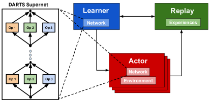
Figure 1: DARTS is potentially a natural fit for RL, as a DARTS supernet can simply be inserted into the network components of a standard RL training pipeline, which may potentially be highly distributed.

Over the past few years, Differentiable Architecture Search (DARTS) (Liu et al.,, 2019) has dramatically risen in popularity as a method for neural architecture search (NAS), with multiple modifications and improvements (Chu et al., 2020c, ; Li et al.,, 2021; Chu et al., 2020a, ; Liang et al.,, 2019; Wang et al., 2021a, ; Chu et al., 2020b, ; Hundt et al.,, 2019; Wang et al., 2021b, ; Chen and Hsieh,, 2020; Zela et al.,, 2020) constantly proposed at a rapid speed. From a broader perspective, one may wonder how far we may push the limits of differentiable search, as differentiability is the cornerstone of all deep learning research. One such very large application space is in reinforcement learning (RL), with DARTS being a natural fit due to its simplicitly and modularity in integrating with large distributed RL training pipelines. Shockingly however, among the vast amounts of literature on DARTS, there are virtually no works addressing its viability in RL.

This can be attributed to the fact that RL fundamentally does not follow the same optimization paradigm as supervised learning (SL). The end goal of RL is not to simply minimize the loss or accuracy over a fixed dataset, but rather to improve a policy’s reward over an entire environment whose training data is generated by the policy itself. This scenario raises the possibility of a negative feedback loop in which a poorly trained policy may achieve trivial reward even if it successfully optimizes its loss to zero, and thus the loss is not an indicator of a policy’s true performance. As DARTS is purely reliant on optimizing the architecture topology by using only the loss as the search signal, therein lies the simple question: Would DARTS even work in RL?

It is highly valuable to answer this question, as recently, works in larger-scale RL suggest that policy architecture designs greatly affect various metrics such as generalization, transferrability, and efficiency. One surprising phenomenon found on Procgen (Cobbe et al.,, 2020), a procedural generation benchmark for RL, was that "IMPALA-CNN", a residual convolutional architecture from (Espeholt et al.,, 2018), could substantially outperform "NatureCNN", the standard 3-layer architecture used for Atari (Mnih et al.,, 2013), in both generalization and sample complexity under limited and infinite data regimes respectively (Cobbe et al.,, 2019). Furthermore, in robotics subfields such as grasping (Kalashnikov et al.,, 2018; Rao et al.,, 2020), cameras collect very detailed real-world images (ex: 472 x 472, 4x larger than ImageNet (Russakovsky et al.,, 2015)) for observations which require deep image encoders consisting of more than 15 convolutions, raising concerns on efficiency and speed in policy training and inference. As such RL policy networks gradually become larger and more sophisticated, so does the need for understanding and automating such designs.

In this paper, we show that DARTS can in fact find better architectures efficiently in RL, one of the first instances in which the loss does not directly affect the final objective. This work may be of interest to both the gradient-based NAS community as means to expand to the RL domain, and the AutoRL community as a practical toolset and method for co-training policies and neural architectures for better performing agents. Our contributions are:

• We conceptually identify the key differences between SL and RL in terms of their usage of the loss function, which raise important hypothetical questions and issues about whether DARTS is applicable to RL. In particular, these deal with the quality of the training signal to the architecture variables during supernet training, and downstream effects on discrete cells during evaluation.

• Empirically, we find that DARTS is in fact compatible with several on-policy and off-policy algorithms including PPO (Schulman et al.,, 2017), Rainbow-DQN (Hessel et al.,, 2018), and SAC (Haarnoja et al.,, 2018). The discrete architectures found can reach up to 250% performance compared to manual architecture designs on discrete action (e.g. Procgen) and continuous control (e.g. DM-Control) environments, at only 3x more computation time.

• Through comprehensive ablation studies, we show the supernet successfully trains, and reasonably upweights optimal operations. We further verify both qualitatively and quantitatively that discretized cells gradually evolve to better architectures. However, we also demonstrate how this can fail, especially if the corresponding supernet fails to train, with further extensive ablations in the Appendix.

Related Works

Recently, there have been a flurry of works modifying many components in the RL pipeline, both manually and automatically, as part of the broader Automated Reinforcement Learning (AutoRL) (Parker-Holder et al.,, 2022) field. Specifically for architecture components, manual modifications include (Raileanu and Fergus,, 2021; Nafi et al.,, 2021; Tang and Ha,, 2021) which have shown great success in improving metrics such as sample complexity and generalization, especially on the Procgen benchmark. However, very few works have considered the possibility of actually automating the search for new architectures, i.e. "NAS for RL", specifically for large-scale modern convolutional networks.

Most previous NAS for RL works only involve small policies trained via blackbox/evolutionary optimization methods, which include (Song et al.,, 2021; Gaier and Ha,, 2019; Stanley and Miikkulainen,, 2002; Stanley et al.,, 2009), utilizing CPU workers for forward pass evaluations rather than exact gradient computation on GPUs. Such methods are usually unable to train policies involving more than 10K+ parameters due to the sample complexity of zeroth order methods in high dimensional parameter space (Agarwal et al.,, 2010). The only previous known application of gradient-based routing is (Akinola et al.,, 2021), which searches for the optimal way of combining observation and action tensors together in off-policy QT-OPT (Kalashnikov et al.,, 2018), but does not search for image encoders nor uses the supernet for inference, as it trains using off-policy robotic data collected independently. This leaves the applicability of DARTS to inference-dependent RL as an open question addressed in our work.

2  Problem Overview and Method

DARTS Preliminaries

Since we only use the original DARTS (Liu et al.,, 2019) to reduce confounding factors, we thus give a very brief overview of DARTS to save space. More comprehensive details can be found in Appendix G.5 and the original paper. DARTS optimizes substructures called cells, where each cell contains $I$ intermediate nodes organized in a directed acyclic graph, where each node $x^{(i)}$, represents a feature map, and each edge $(i,j)$ consists of an operation (op) $o^{(i,j)}$, with later nodes $x^{(j)}$ merged (e.g. summation) from some previous $o^{(i,j)}(x^{(i)})$. A DARTS supernet is constructed by continuously relaxing selection of ops in $\mathcal{O}$, via softmax weighting, i.e. $\overline{o}^{(i,j)}(x^{(i)})=\sum_{o\in\mathcal{O}}p_{o}^{(i,j)}\cdot o(x^{(i)})$, where $p_{o}^{(i,j)}=\frac{\exp(\alpha_{o}^{(i,j)})}{\sum_{o^{\prime}\in\mathcal{O}}\exp(\alpha_{o^{\prime}}^{(i,j)})}$. The cell’s output is by default the result of a Conv1x1 op on the depthwise concatenation of all intermediate node features, although this may be changed (e.g. by simply outputting the last intermediate node’s features). We denote the collection of all architecture variables $a_{o}^{(i,j)}$ as $\alpha$. Denote the total set of possible operations in our searchable network as $\mathcal{O}=\mathcal{O}_{base}\cup\{\text{Zero, Skip}\}$ which must contain Zero and Skip Connection ops, while $\mathcal{O}_{base}$ is user-defined. Denote $\alpha$ to be the pre-softmax trainable architecture variables in the supernet. A predefined loss function $\mathcal{L}(\theta)$ over neural network weights $\theta$ will thus be redefined as $\mathcal{L}(\theta,\alpha)$ when under DARTS’s search mode, where the original model $f_{\theta}$ will be replaced with a dense supernet $f_{\theta,\alpha}$. During evaluation time, a trained $\alpha^{*}$ is then discretized into a sparser final cell $\delta(\alpha^{*})$ by representing each edge $(i,j)$ with the highest softmax weighted op, i.e. $\arg\max_{o\in\mathcal{O},o\neq zero}p_{o}^{(i,j)}$, and then retaining only the top $K$ incoming edges for each intermediate node. We thus retrain over the new loss $\mathcal{L}_{\delta(\alpha^{*})}(\phi)$, now dependent on only fresh sparse weights $\phi$ to obtain the final reported metric.

RL Preliminaries

For RL notation, given an MDP $\mathcal{M}$, denote $s_{t},a_{t},r_{t}$ as state, action, reward respectively at time $t$. $\pi$ is the policy and $\mathcal{D}$ is the replay buffer containing collected trajectories $\tau=(s_{0},a_{0},r_{0},s_{1},\ldots)$. The goal is to maximize $J(\pi)=\mathbb{E}_{\tau\sim\pi}\left[\sum_{t\geq 0}r_{t}\right]$, the expected cumulative reward using policy $\pi$. In most RL algorithms, there is the notion of a neural network torso or encoder $f_{\theta}$ mapping the state $s$ to a final feature vector when forming $\pi$. In the DARTS case, we use a supernet encoder $f_{\theta,\alpha}$ leading to a supernet policy denoted as $\pi_{\theta,\alpha}$ and also a corresponding discretized-cell policy $\pi_{\phi,\delta(\alpha^{*})}$ for evaluation.

1. Supernet training: Compute $\alpha^{*}$ from $\operatorname*{arg\,max}_{\theta,\alpha}J(\pi_{\theta,\alpha})$ via $\operatorname*{arg\,min}_{\theta,\alpha}\mathcal{L}^{RL}(\theta,\alpha)$.

2. Discretization: Discretize $\alpha^{*}$ to construct evaluation policy $\pi_{\phi,\delta(\alpha^{*})}$.

3. Evaluation: Report $\max_{\phi}J(\pi_{\phi,\delta(\alpha^{*})})$ via $\operatorname*{arg\,min}_{\phi}\mathcal{L}_{\delta(\alpha^{*})}(\phi).$

Algorithm 1 RL-DARTS Procedure.

2.1  Methodology

SL features the notion of training and validation sets, with corresponding losses $\mathcal{L}^{SL}_{train},\mathcal{L}^{SL}_{val}$, where the learning procedure consists of a bilevel optimization problem and the goal is to find $\alpha^{*}=\operatorname*{arg\,min}_{\alpha}\mathcal{L}^{SL}_{val}(\theta^{*},\alpha)$ where $\theta^{*}=\operatorname*{arg\,min}_{\theta}\mathcal{L}^{SL}_{train}(\theta,\alpha)$. In this paper, we do not need to use the original bilevel optimization framework, as we are optimizing sample complexity and raw training performance, which are standard metrics in RL. Furthermore, bilevel optimization is notoriously difficult and unstable, sometimes requiring special techniques (Liu et al.,, 2018; Dong and Yang,, 2019; Hundt et al.,, 2019; Li et al.,, 2020; Chu et al., 2020b, ; Chu et al., 2020a, ; Chu et al., 2020c, ; Liang et al.,, 2019; Wang et al., 2021b, ) specific to SL optimization, which can confound the results and message of our paper.

We thus joint optimize both $\theta$ and $\alpha$, and the full procedure is concisely summarized in Algorithm 1 as "RL-DARTS". However, this is easier said than done, as we explain the core issues of applying DARTS to RL below.

SL vs RL DARTS

Fundamentally, SL relies on a fixed dataset $\mathcal{D}^{SL}=\{(x_{i},y_{i})\>\>|\>\>i\geq 1\}$, in which the loss is defined as $\mathcal{L}^{SL}(\theta)=\mathbb{E}_{(x,y)\sim\mathcal{D}}\left[\ell(f_{\theta}(x),y)\right]$ where $\ell(\cdot)$ is defined as mean squared error, cross-entropy loss, or negative log-likelihood depending on application. These losses are strongly correlated or even equivalent to the final objective (e.g. accuracy or density estimation), and this reason can be considered a significantly contributing factor to the success of DARTS in SL. Unfortunately in RL, there are no such guarantees that minimizing the loss $\mathcal{L}^{RL}(\cdot)$ necessarily improves the true objective $J(\cdot)$, for two primary reasons:

1. The RL agent’s dataset (a.k.a. replay buffer) $\mathcal{D}^{RL}=\{\tau_{i}\>\>|\>\>i\geq 1\}$ is significantly non-stationary and self-dependent, as it constantly changes based on the current performance of data collection actors, which themselves are functions of $\theta$. Thus, a negative feedback loop may arise, where $\theta$ produces an actor which collects poor training data, leading to convergence towards an even poorer $\theta^{\prime}$. While the loss $\mathcal{L}^{RL}(\cdot)$ converges to 0 over low quality data, the reward $J(\cdot)$ still does not increase. This issue is commonplace in RL, such as in any environments which require exploration. Hypothetically in the DARTS case, $\alpha$ can potentially produce the same negative feedback loop by converging to subpar operations and impairing supernet training, also leading to a poor discrete cell $\delta(\alpha)$.

2. The losses are considerably more complex and utilize multiple auxiliary losses which are used to assist training but never used during evaluation. For PPO, the loss is defined as $\mathcal{L}^{RL}_{PPO}(\theta)=\mathbb{E}_{\tau\sim\mathcal{D}_{RL}}\left[L_{CLIP}(\theta)-L_{VF}(\theta)+\mathcal{H}(\theta)\right]$. However, the value function (corresponding to $L_{VF}$) nor the policy entropy (corresponding to $\mathcal{H}$) are never used to evaluate final reward. This is similarly the case for off-policy algorithms such as SAC which strongly emphasizes maximizing the entropy $\mathcal{H}$ and Rainbow-DQN which also uses value functions to assist training. The question is thus raised in the DARTS case as to whether such auxiliary losses are actually useful signals, or inhibit proper training of $\alpha$, whose main goal is only maximize $J(\cdot)$ using discrete cell $\delta(\alpha)$.

The core theme of our experiments will be understanding whether these are obstacles to DARTS’s application to RL.

3  Experiments

Experiment Setup: To verify that every component of RL-DARTS works as intended, we seek to answer all questions below, by first presenting end-to-end results, and then further key ablation studies:

1. End-to-End Performance: Overall, how do the final discrete cells perform at evaluation, and what gains can we obtain from architecture search? Furthermore, how does RL-DARTS compare against random search?

2. Supernet Training: During supernet training, how does the $\alpha$ change? Does $\alpha$ converge towards a sparse solution and select good operations over supernet training?

3. Discrete Cells: Even if the supernet trains, do the corresponding discrete cells also improve in evaluation performance throughout $\alpha$’s training? What kinds of failure modes occur?

Following common NAS practices (Zoph et al.,, 2018; Pham et al.,, 2018; Zoph and Le,, 2016), we construct our supernet (with $I$ intermediate cells) by stacking both normal ($N$ times) and reduction cells ($R$ times) together into blocks, which are themselves also stacked together $D$ times (see Figure 2). Reduction cells apply a stride of 2 on the input. Each block possesses its own convolutional channel depth, used throughout all cells in the block. During search, we train a smaller supernet (i.e. depth 16) to reduce computation time, but evaluate final discretized cells on larger models (i.e. depth 64), with $D=3$ layers for cheap large-scale runs and $D=5$ layers for fine-grained A/B testing.

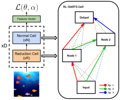
Figure 2: Illustration of our network via stacking normal and reduction cells. Solid lines correspond to selected ops after discretization from all possible ops weighted using $\alpha$. If $R>0$, we add an initial Conv3x3 for preprocessing.

For the operation search space, we consider the following base ops $\mathcal{O}_{base}$ and corresponding algorithms:

• Classic on PPO: $\mathcal{O}_{base,N}$ = {Conv3x3+ReLU, Conv5x5+ReLU, Dilated3x3+ReLU, Dilated5x5+ReLU} for normal ops and $\mathcal{O}_{base,R}$ = {Conv3x3, MaxPool3x3, AveragePool3x3} for reduction ops, which is standard in supervised learning (Liu et al.,, 2019; Zoph et al.,, 2018; Pham et al.,, 2018).

• Micro on Rainbow and SAC: We also propose $\mathcal{O}_{base,N}$ = {Conv3x3, ReLU, Tanh}, a more fine-grained and novel search space which has not been used previously in SL. The inclusion of Tanh is motivated by its use previously for continuous control architectures (Salimans et al.,, 2017; Song et al.,, 2020).

For benchmarks, we primarily use Procgen (Cobbe et al.,, 2019, 2020) for discrete action spaces, with PPO (Schulman et al.,, 2017) and Rainbow DQN (Hessel et al.,, 2018) as training algorithms, with Procgen’s difficulty set to "easy" similar to other works (Raileanu et al.,, 2020; Raileanu and Fergus,, 2021; Parker-Holder et al., 2021a, ). Procgen comprehensively evaluates all aspects of RL-DARTS, as it possesses a diverse selection of 16 games, each with infinite levels to simulate large data regimes where episodes may drastically change, relevant for generalization. It further uses the IMPALA-CNN architecture (Espeholt et al.,, 2018) as a strong hand-designed baseline, and can be seen as a specific instance of the stacked cell design in Figure 2, where its "Reduction Cell" consists of a Conv3x3 and MaxPool3x3 (Stride 2) with $R=1$ and its "Normal Cell" consists of a residual layer with Conv3x3’s and ReLU’s, with $N=2$. For fair comparisons to IMPALA-CNN, we use $(N,R,I)=(1,1,4)$ on the classic search space, while $(N,R,I)=(2,0,4)$ on the Micro search space, where reduction ops default to IMPALA-CNN’s in order to avoid hidden confounding effects when visualizing Micro cells.

In addition, we also assess DARTS’s viability in continuous control which is common in robotics tasks. We use the common DM-Control benchmark (Tassa et al.,, 2018) along with the popular SAC algorithm. We use $N=3,I=4,K=1$ with "Micro" search space to remain fair to the 4-layer convolutional encoder baseline observing images of size $64\times 64$ (full details in Appendix G).

Unless specified, we by default use consistent hyperparameters (found in Appendix G) for all comparisons found inside a figure, although learning rate and minibatch size may be altered when training models of different sizes due to GPU memory limits. Thus, even though RL is commonly sensitive to hyperparameters (Zhang et al.,, 2021), we surprisingly find that once a pre-existing RL baseline has already been setup, incorporating DARTS requires no extra cost in tuning, as evidence of its ease-of-use.

3.1  End-to-End Results on Multi-task, Discrete and Continuous Control Tasks

Multi-game Search

We first begin with the most surprising and largest end-to-end result in terms of scale of data and compute shown in Figure 3: By training a supernet across infinite levels across all 16 Procgen games to find a single transferrable cell, we are able to achieve up to $250\%$ evaluation performance compared to the IMPALA-CNN baseline over select environments. This is achieved using Rainbow with our proposed "Micro" search space, where a learner performs gradient updates over actor replay data (with normalized rewards) from all games.

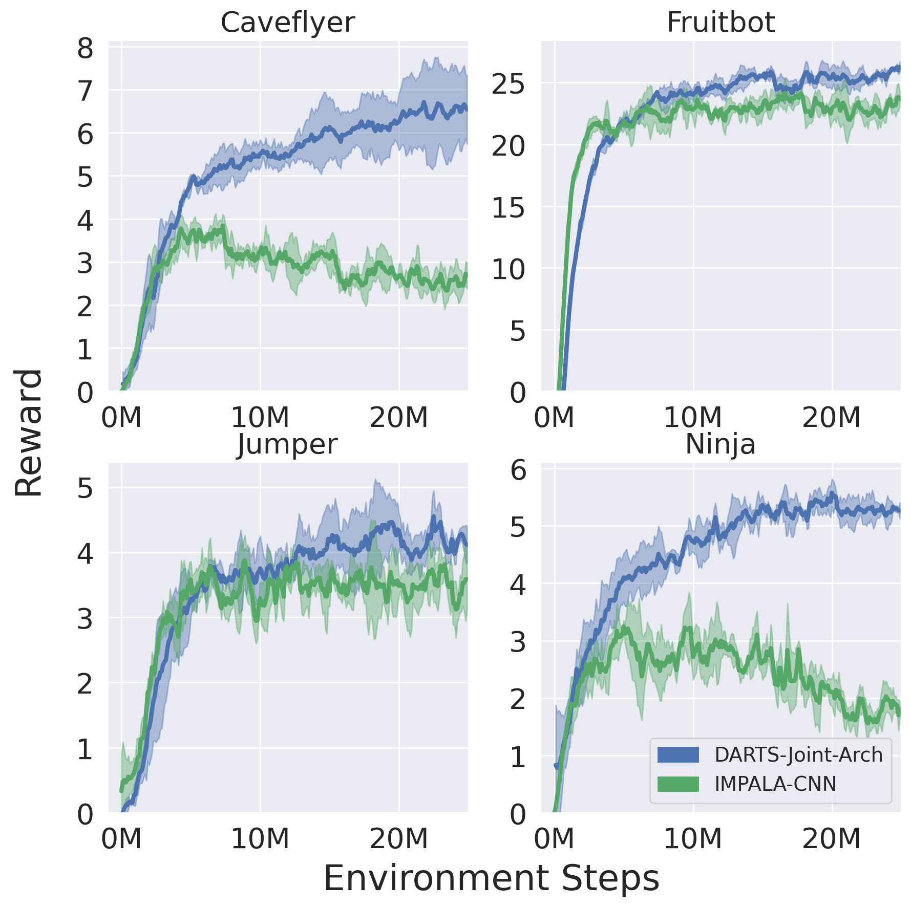
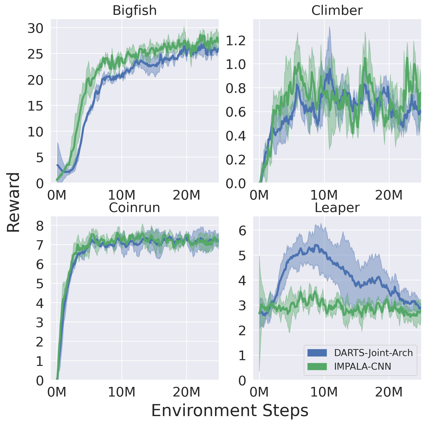
Figure 3: Evaluation of the discrete cell joint-trained over 8 environments using depths $64\times 5$ to emphasize comparison differences.

We further display the discovered discrete cell and the supernet joint-training procedure in Figure 4. Interestingly, the discrete cell uses nonlinearities over all intermediate connections, with convolutions only used via the merge operation for the output.

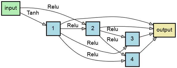
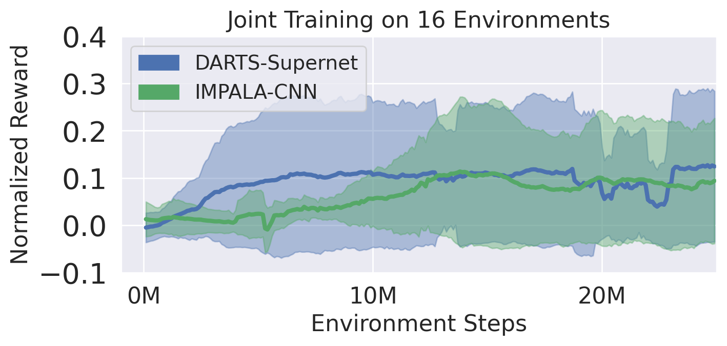
Figure 4: Left: Discrete cell found. Right: Average normalized rewards over all 16 games during supernet + baseline training.

Single-game Search

We further compare DARTS’s end-to-end performance against random search, but more appropriately applied to single game scenarios. On the PPO side, we use the "Classic" search space (total size $4\times 10^{11}$, see Appendix H.1). For a fair comparison, we ensure total wall-clock time (with same hardware) stays equal, as common in (Liu et al.,, 2019). Since in Appendix A, Table 4, a PPO supernet takes 2.5x longer to reach 25M steps, this is rounded to a random search budget of 3 cells to be trained with depths $16\times 3$ for 25M steps. The best of the 3 cells is used for full evaluation. In Table 1, on average, random search underperforms significantly.

	IMPALA-CNN	RL-DARTS (Discrete Cell)	Random Search
Avg. Normalized Reward	0.708	0.709	0.489

Table 1: Average normalized rewards across all 16 environments w/ PPO, using the normalization method from (Cobbe et al.,, 2020). Full details and results (including Rainbow) are presented in Appendix E.

In Figure 5 we further find that RL-DARTS is capable of finding game-specific architectures from scratch which outperform IMPALA-CNN on select environments such as Plunder and Heist, while maintaining competitive performance on others.

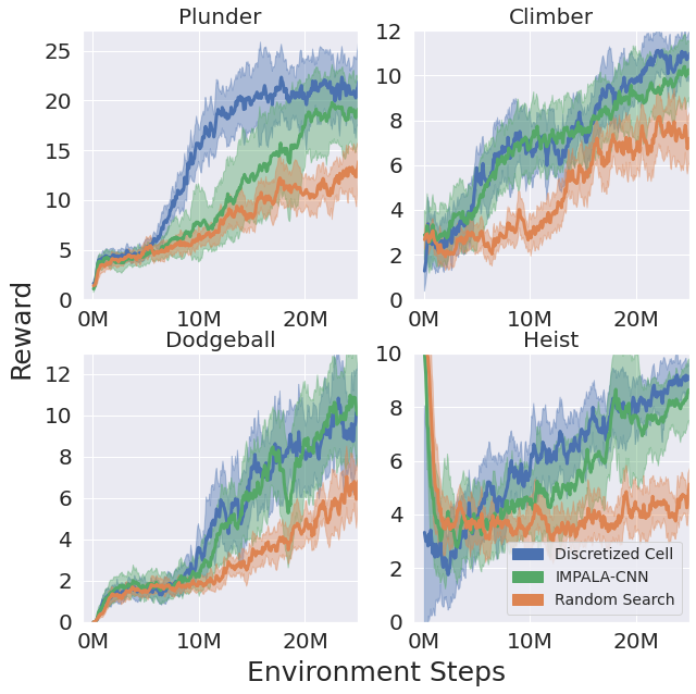
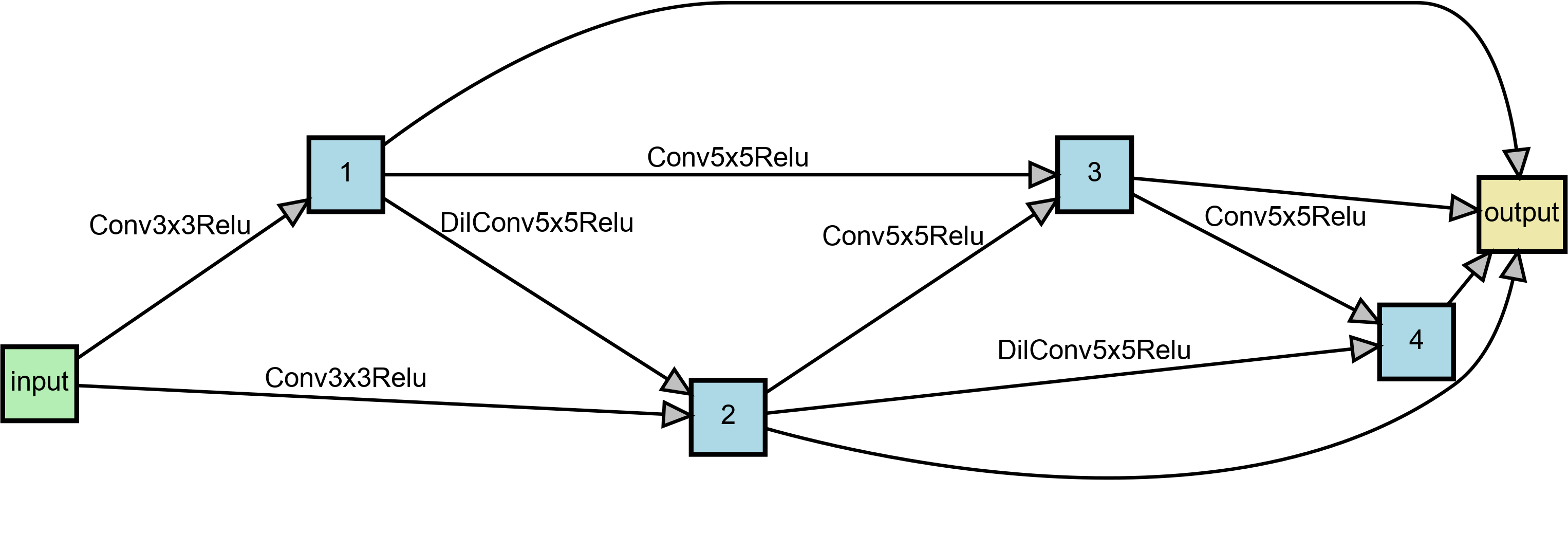
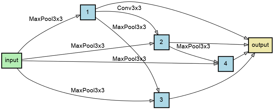
Figure 5: Left 2x2 Plot: Examples of discrete cell evaluations using the "Classic" search space with PPO, with depths $64\times 3$. Right: Normal (Top) and Reduction (Bottom) cells found for "Plunder" which achieves faster training than IMPALA-CNN. Note the interesting use of 5x5 convolutional kernel sizes later in the cell.

100 Random Cell Comparison

To further present a more comprehensive comparison against random search, and understand how strong IMPALA-CNN is as a baseline, we compare against 100 unique random cells. To manage the computational load, we performed the study over two selected environments, as shown in Figure 6 and find that all of the random cells underperform against both IMPALA-CNN and DARTS. This demonstrates that DARTS possesses a strong search capability, achieving $100/3\approx 30x$ efficiency over random search and can discover architectures that match in complexity and performance of highly-tuned, expert designed architectures such as IMPALA-CNN.

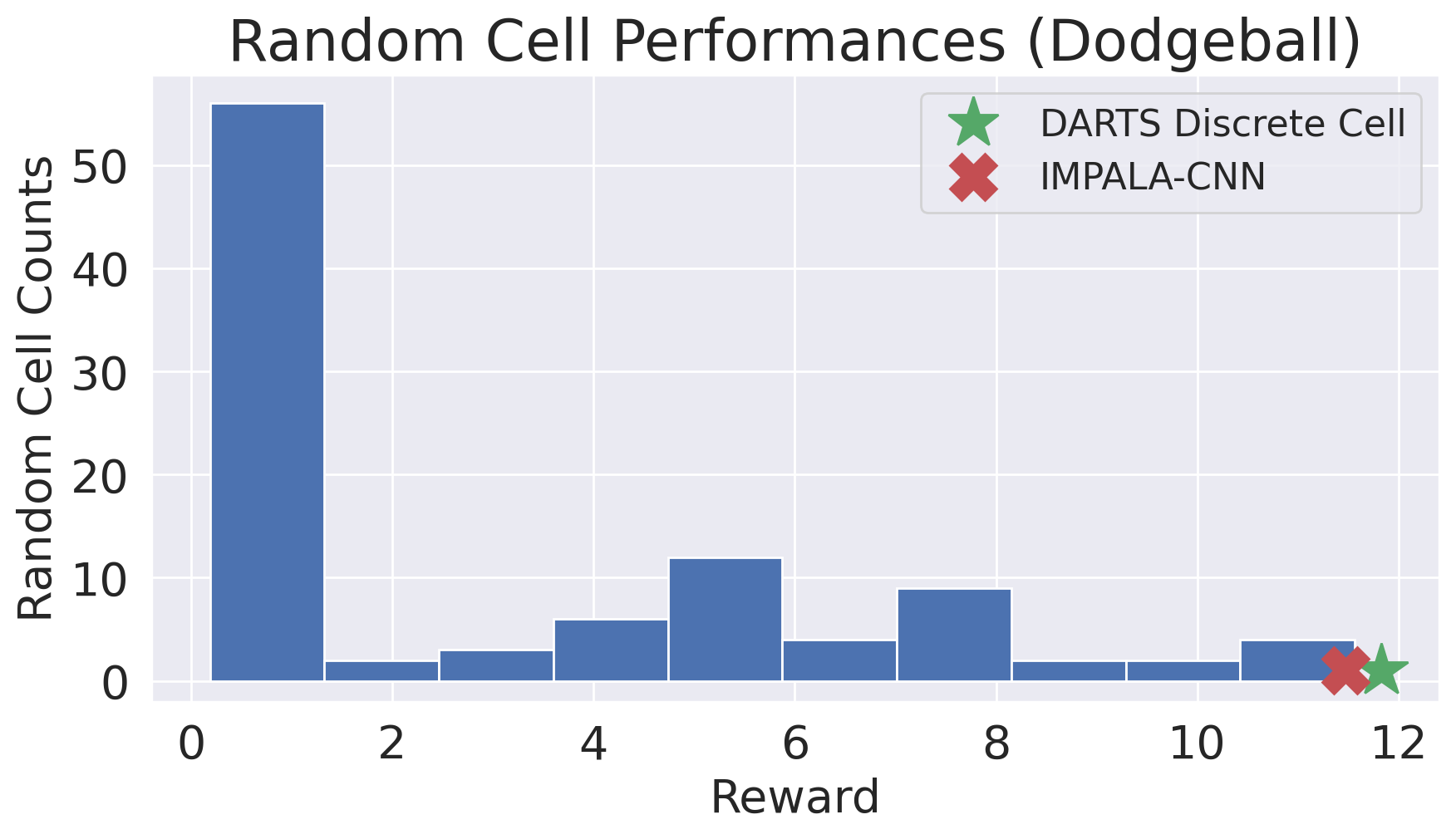
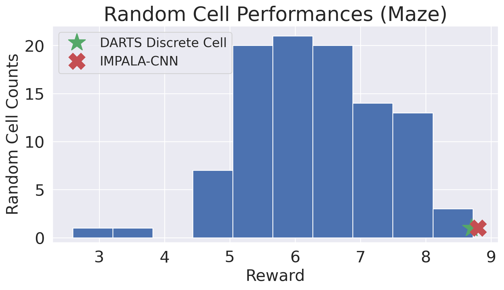
Figure 6: Histogram of 100 random cells’ rewards over environments Dodgeball and Maze using the Rainbow + "Micro" search space (depths $64\times 3$), with a significant number of random cells (e.g. 95% for Dodgeball) performing substantially worse than DARTS or IMPALA-CNN.

DM-Control with Soft Actor-Critic

DARTS also consistently finds better and stable architectures over multiple lightweight environments involving continuous control (see Figure 7) trained up to 1M steps. Even though the 4-layer encoder network used (details in Appendix G) is significantly smaller than IMPALA-CNN, we find that there is still room for architectural improvement.

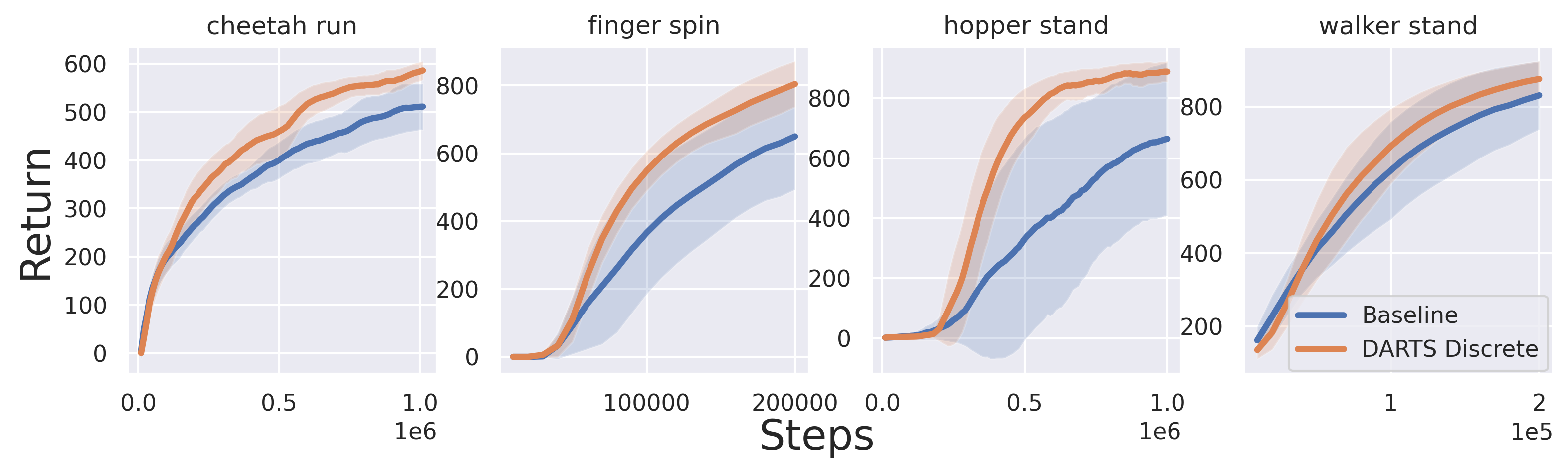
Figure 7: RL-DARTS on DM-Control with SAC also finds better architectures over the corresponding baseline.

3.2  Role of Supernet Training

In Figure 8, we verify that training the supernet end-to-end works effectively, even with minimal hyperparameter tuning. Furthermore, the training only requires at 3x more compute time, with extensive efficiency metrics calculated in Appendix A. However, as mentioned in Subsec. 2.1, it is unclear whether the right signals are provided to operation routing variables $\alpha$ via the RL training loss, and whether $\alpha$ produces the correct behavior, which we investigate.

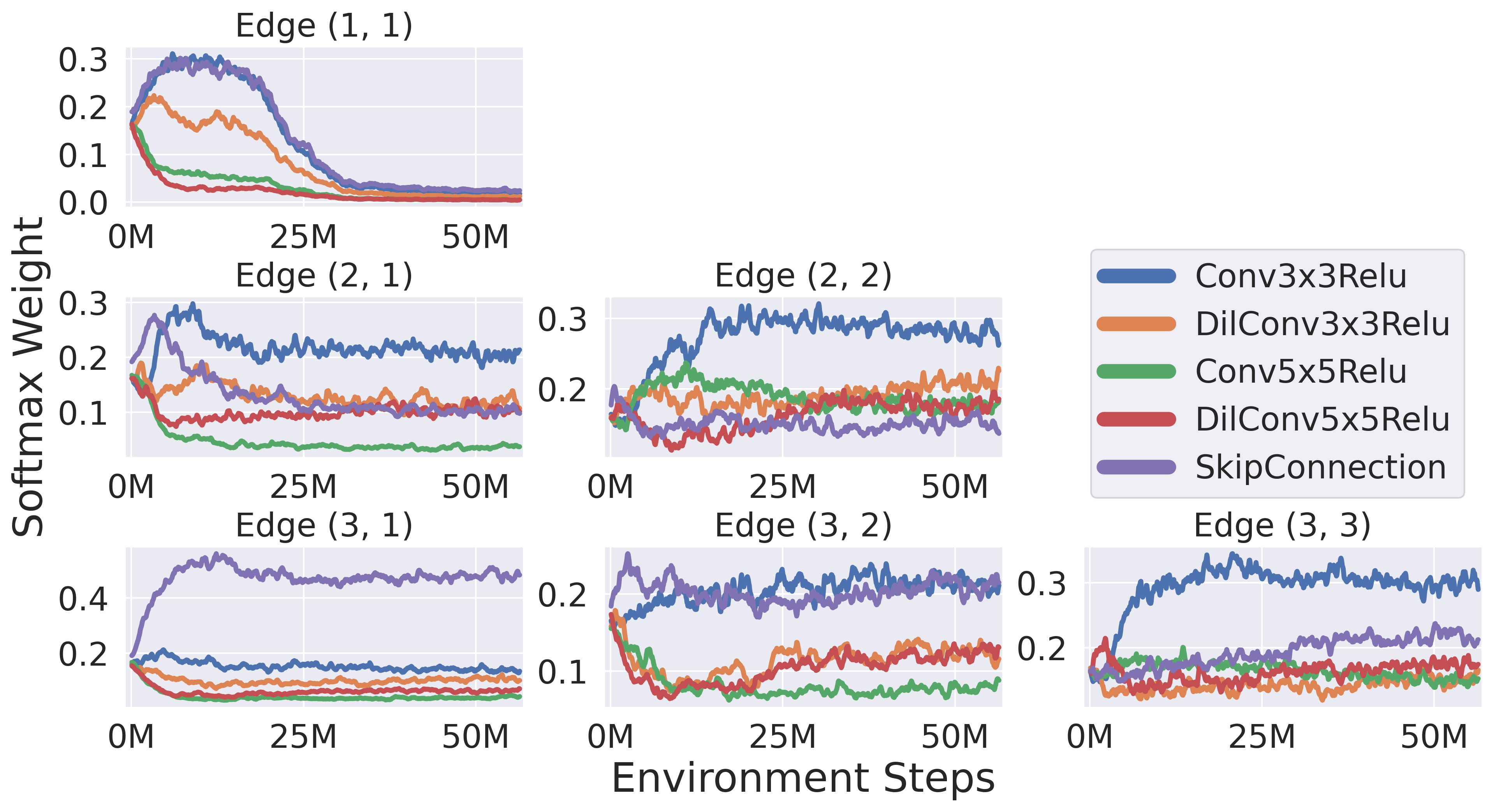
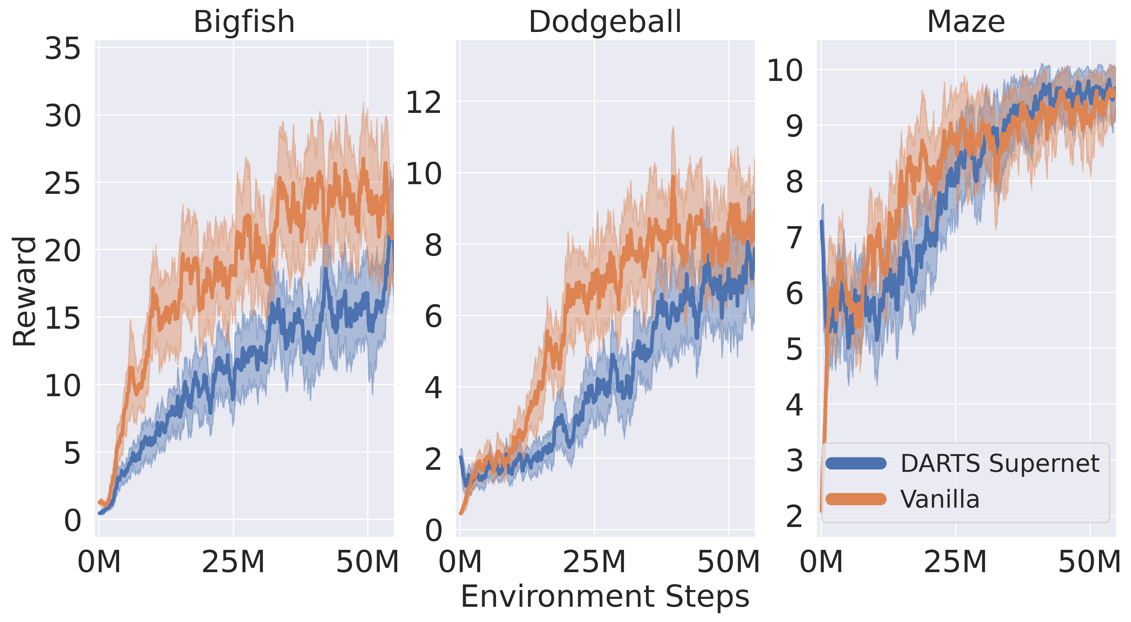
Figure 8: Left: Softmax op weights over all edges in the cell when training the supernet with PPO + "Classic" search space on Dodgeball. Zero op weight is not shown to improve clarity. Right: Sanity check to verify that the supernet eventually achieves a regular training curve, using vanilla IMPALA-CNN as a rough gauge. Both use depths $16\times 3$. Note that while we show the curve up to 50M steps, we by default discretize $\alpha$ at 25M steps, as op choices have already converged towards a sparser solution. Analogous figure for Rainbow in Appendix B.

Conveniently in Figure 8, we find that $\alpha$ strongly downweights all base ops (in particular, 5x5 ops) except for the standard Conv3x3+ReLU. This provides an opportunity to understand whether $\alpha$ downweights suboptimal ops throughout training. We confirm this result in Table 2 by evaluating standard IMPALA-CNN cells using either purely 3x3 or 5x5 convolutions for the whole network, and demonstrating that the 3x3 setting outperforms the 5x5 setting (especially in limited data, e.g. 200-level training/test regime), suggesting the signaling ability of $\alpha$ on op choice.

Scenario	Conv 3x3	Conv 5x5
Train (Inf. levels)	15.1 $\pm$ 2.5	13.2 $\pm$ 2.3
Train (200 levels)	12.1 $\pm$ 1.7	9.8 $\pm$ 2.1
Test (from Train)	10.2 $\pm$ 2.3	5.9 $\pm$ 1.7

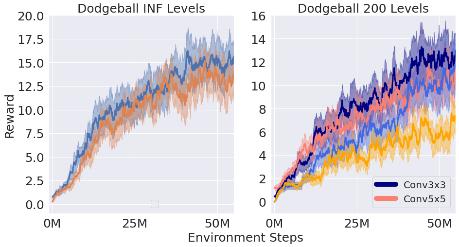
Figure 15: Large IMPALA-CNNs evaluated on Dodgeball using either Infinite or 200 levels with PPO. For the 200 level setting, lighter colors correspond to test performance.

Table 2: PPO IMPALA-CNN evaluations (mean return at 50M steps) on Dodgeball. Learning curves can be found in Appendix D.1, Figure 15.

Answering the converse question is just as important: Can any supernet train? The supernet possesses an incredibly dense set of weights, and thus one might wonder whether trainability occurs with any search space or settings. We answer in the negative, where a poorly designed supernet can fail. To show this clearly, we remove all ReLU nonlinearities from the "Classic" search space ops used for PPO, as well as simply freeze $\alpha$ to be uniform for Rainbow, and find both cases produce poor training in Table 3. Thus, the supernet in RL provides important search signals in terms of reward and $\bm{\alpha}$ during training, especially on the quality of a search space.

	Rainbow (25M Steps)		PPO (50M Steps)
Scenario	Trainable $\alpha$	Uniform $\alpha$	With ReLU	No ReLU
Training (Inf. levels) Reward	3.1 $\pm$ 0.5	0.9 $\pm$ 0.2	7 $\pm$ 0.9	1.9 $\pm$ 0.3

Table 3: Supernet training rewards on Dodgeball. Learning curves can be found in Appendix C.

3.3  Discrete Cell Improvement

We further must analyze whether discrete cells also improve, as they are used for final evaluation and deployment. Strong supernet performance (via continuous relaxation) does not necessarily imply strong evaluation cell performance (via discretization), due to the existence of integrality gaps (Wang et al., 2021b, ; Wang et al., 2021a, ). Nevertheless, we demonstrate that even using the default $\delta$ discretization from (Liu et al.,, 2019) leads to both quantitative and qualitative improvements.

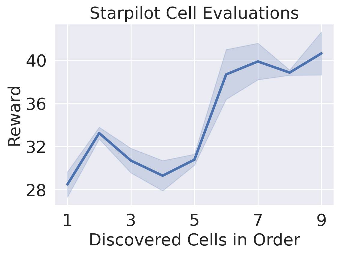
Figure 9: Evaluation of 9 distinct discrete cells in order from the trajectory of $\alpha$ on the Starpilot environment when using Rainbow.

Quantitative improvement

As $\alpha$ changes during supernet training, so do the outputs of the discretization procedure on $\alpha$. We collect all distinct discrete cells $\{\delta(\alpha_{1}),\delta(\alpha_{2}),\ldots\}$ into a sequence, and evaluate each cell’s performance $\max_{\phi}J(\pi_{\phi,\delta(a_{i})})\>\>\forall i$ via training from scratch for 25M steps (Figure 9). The performance generally improves over time, indicating that supernet optimization selects better cells. However, we find that such behavior can be environment-dependent, as some environments possess less monotonic evaluation curves (see Fig. 18 in Appendix D).

Qualitative improvement

We visualize discrete cells $\delta(\alpha_{start}),\delta(\alpha_{end})$ from the start and end of supernet training with Rainbow on the Starpilot environment in Fig. 10. The earlier cell consists of only linear operators is clearly a poor design in comparison to the later cell. We find similar cell evolution results for PPO in Figures 16, 17 in Appendix D.2, displaying more sophisticated yet still interpretable changes in cell topology.

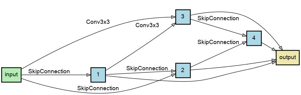
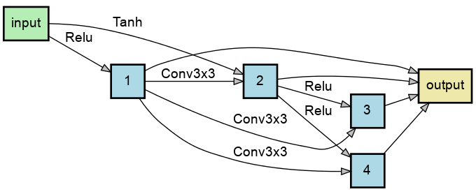
Figure 10: Evolution of discovered cells over a DARTS optimization process. Left: $\delta(\alpha_{start})$ discovered in the early stage which is dominated by skip connections and only linear ops. Right: $\delta(\alpha_{end})$ discovered in the end which possesses several reasonable local structures similar to Conv + ReLU residual connections.

We further answer one of the most common questions in DARTS research: What is the direct relationship between a supernet and its discrete cell? In Figure 11, we provide two supernet runs along with their corresponding discrete cells, side by side in order to answer this question. While "Supernet 1" is a standard successful training run, "Supernet 2" is a failed run which can commonly occur due to the inherent sensitivity and variance in RL training. As it turns out, this directly leads to differences between their corresponding discrete cells both quantitatively and qualitatively as well, in which "Discretized Cell 1"’s design appears to make sense and train properly, while "Discretized Cell 2" is clearly a suboptimal design, and fails to train at all. Thus, a major reason for why a discretized cell may underperform is if its corresponding supernet fails to learn.

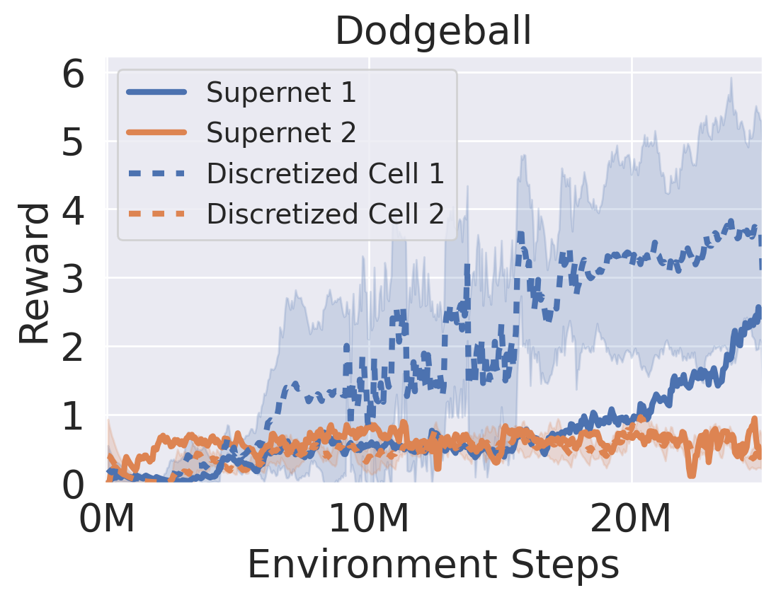
(a) Different supernet runs, with corresponding discretized cell (depths $64\times 5$) training curves.

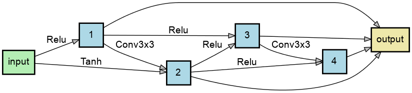
(b) Discretized Cell 1

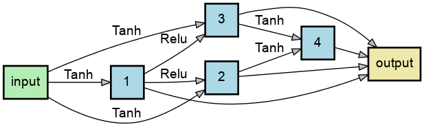
(c) Discretized Cell 2

Figure 11: (a) Two different supernets trained on the Dodgeball environment using Rainbow, with corresponding discretized cells evaluated using 3 random seeds. (b) Discretized cell from Supernet 1. Note the similarity to regular Conv3x3 + ReLU designs. (c) Discretized cell from Supernet 2, which uses too many Tanh nonlinearities, known to cause vanishing gradient effects.

We investigate further in Appendix D.3, Figure 19, and find that supernet and discrete cell rewards are indeed correlated, after adjusting for environment-dependent factors, suggesting that search quality can be improved via both better supernet training (Raileanu et al.,, 2020; Zhang et al.,, 2021), as well as better discretization procedures (Liang et al.,, 2019; Wang et al., 2021b, ).

4  Conclusions, Limitations, and Broader Impact Statement

Conclusion

Even though RL uses complex loss functions defined over nonstationary data, we empirically showed that nonetheless, DARTS is capable of improving policy architectures in a minimally invasive and efficient way (only 3x more compute time) across several different algorithms (PPO, Rainbow, SAC) and environments (Procgen, DM-Control). Our paper is the first to have comprehensively provided evidence for the applicability of softmax/gradient-based architecture search outside of standard classification and SL.

Limitations

To avoid confounding factors and for simplicity, our paper uses the default DARTS method. However, we outline multiple possible improvements in Appendix F, as RL is a completely new frontier for which to understand softmax routing and continuous relaxation techniques.

Future Work and Broader Impact

In this paper, we have provided concrete evidence that architecture search can be conducted practically and efficiently in RL, via DARTS. We believe that this could start important initiatives into finding better and more efficient (Cai et al.,, 2019) architectures for large-scale robotics (James et al.,, 2019; Akinola et al.,, 2021), transferable architectures in offline RL (Levine et al.,, 2020), as well as RNNs for memory (Pritzel et al.,, 2017; Fortunato et al.,, 2019; Kapturowski et al.,, 2019) and adaptation (Duan et al.,, 2016; Wang et al.,, 2017). Other NAS methods’ applicability in RL may also be investigated, especially ones which utilize blackbox optimization controllers, such as multi-trial evolution (Real et al.,, 2019) or ENAS (Pham et al.,, 2018).

Furthermore, we believe our work’s potential negative impacts are generally equivalent to ones found in general NAS methods, such as sacrificing model interpretability in order to achieve higher objectives. For the field of RL specifically, this may warrant more attention in AI safety when used for real world robotic pipelines. Furthermore, as with any NAS research, the initial phase of discovery and experimentation may contribute to carbon emissions due to the computational costs of extensive tuning. However, this is usually a means to an end, such as an efficient search algorithm, which this paper proposes with no extra hardware costs.

5  Reproducibility Checklist

1. For all authors…

   1. Do the main claims made in the abstract and introduction accurately reflect the paper’s contributions and scope? [Yes] We have comprehensively demonstrated the behavior of all components in DARTS when applied inside an RL pipeline.

   2. Did you describe the limitations of your work? [Yes] Yes, see Section 4.

   3. Did you discuss any potential negative societal impacts of your work? [Yes] Yes, see Section 4.

   4. Have you read the ethics review guidelines and ensured that your paper conforms to them? [Yes] Yes, see Section 4.

2. If you are including theoretical results…

   1. Did you state the full set of assumptions of all theoretical results? [N/A] No theoretical results provided.

   2. Did you include complete proofs of all theoretical results? [N/A] No proofs provided.

3. If you ran experiments…

   1. Did you include the code, data, and instructions needed to reproduce the main experimental results, including all requirements (e.g., requirements.txt with explicit version), an instructive README with installation, and execution commands (either in the supplemental material or as a url)? [Yes] We have included the core code for creating a DARTS supernet and discrete cell, as well as training code for Procgen on both PPO and Rainbow, and addition added the modified files from an open-source variant of SAC on DM-Control. We have also added the README on guidance for code organization and running experiments, as well as a requirements.txt. The code can be found at https://github.com/google/brain_autorl/tree/main/rl_darts.

   2. Did you include the raw results of running the given instructions on the given code and data? [Yes] We have provided the data related to the core results of this paper.

   3. Did you include scripts and commands that can be used to generate the figures and tables in your paper based on the raw results of the code, data, and instructions given? [Yes] We have provided relevant figure-plotting utilities in the code submission.

   4. Did you ensure sufficient code quality such that your code can be safely executed and the code is properly documented? [Yes] The code was formatted by a strict automatic Python lint-checker, as well as reviewed by other individuals. The code also provides tests for modules, which can be used to understand the intended use.

   5. Did you specify all the training details (e.g., data splits, pre-processing, search spaces, fixed hyperparameter settings, and how they were chosen)? [Yes] We discuss the explicit hyperparameters in Appendix G, as well as search space details in Section 3.

   6. Did you ensure that you compared different methods (including your own) exactly on the same benchmarks, including the same datasets, search space, code for training and hyperparameters for that code? [Yes] We ensured the same evaluation protocol via making sure all depths remain the same ($16$ for supernets, $64$ for discrete cells, and $D=3$ layers for cheaper large-scale runs or $D=5$ for fine-grained A/B testing). We also used the exact same hyperparameters for all discrete/baseline runs, while only needing to change minibatch size + learning rate in accomodate networks with larger GPU memory sizes.

   7. Did you run ablation studies to assess the impact of different components of your approach? [Yes] For ablation studies, we provided a large set of studies as seen throughout Subsections 3.2 and 3.3 as well as in the Appendix.

   8. Did you use the same evaluation protocol for the methods being compared? [Yes] In terms of comparing NAS methods, we indeed controlled for confounding factors by using the same hardware, as shown in Table 4 in Appendix A. We further performed side-by-side comparisons for RL training curves using environment steps, which is standard.

   9. Did you compare performance over time? [Yes] Table 4 in Appendix A contains wall-clock time comparisons. In terms of performance comparisons over time, we showed the performance of RL-DARTS’s discrete cells over the search procedure / supernet training in Figure 9.

   10. Did you perform multiple runs of your experiments and report random seeds? [Yes] For seeded runs, as standard in RL, we performed 3-seeded runs for all experiments.

   11. Did you report error bars (e.g., with respect to the random seed after running experiments multiple times)? [Yes] For seeded runs, as standard in RL, we performed 3-seeded runs for all experiments and reported error bars.

   12. Did you use tabular or surrogate benchmarks for in-depth evaluations? [Yes] We extensively covered the comparisons against random search in Subsection 3.1, over all 16 games as well as a large scale 100 random cell comparison in Figure 6.

   13. Did you include the total amount of compute and the type of resources used (e.g., type of gpus, internal cluster, or cloud provider)? [Yes] See Table 4 in Appendix A for GPU and compute time used for all evaluations. We applied this to all 16 games on Procgen.

   14. Did you report how you tuned hyperparameters, and what time and resources this required (if they were not automatically tuned by your AutoML method, e.g. in a nas approach; and also hyperparameters of your own method)? [Yes] This is written in detail in Appendix G as well as Section 3.

4. If you are using existing assets (e.g., code, data, models) or curating/releasing new assets…

   1. If your work uses existing assets, did you cite the creators? [Yes] We have cited Procgen and DM-Control.

   2. Did you mention the license of the assets? [N/A] Both are publicly licensed and freely available.

   3. Did you include any new assets either in the supplemental material or as a url? [Yes] We included the relevant publicly available code for environments and algorithms in Section G.

   4. Did you discuss whether and how consent was obtained from people whose data you’re using/curating? [N/A] Benchmarks are publicly available, consent not needed.

   5. Did you discuss whether the data you are using/curating contains personally identifiable information or offensive content? [N/A] No personally identifiable information or offensive content.

5. If you used crowdsourcing or conducted research with human subjects…

   1. Did you include the full text of instructions given to participants and screenshots, if applicable? [N/A] No research was conducted on human subjects or crowdsourcing.

   2. Did you describe any potential participant risks, with links to Institutional Review Board (irb) approvals, if applicable? [N/A] No research was conducted on human subjects or crowdsourcing.

   3. Did you include the estimated hourly wage paid to participants and the total amount spent on participant compensation? [N/A] No research was conducted on human subjects or crowdsourcing.

Appendix

Appendix A Efficiency Metrics

We provide computational efficiency metrics in Table 4, where we find that the practical wall-clock time required for training the supernet (i.e. the search cost) is very comparable with DARTS in SL (Liu et al.,, 2019), requiring only a few GPU days. We do note that unlike SL where the vast majority of the cost is due to the network, RL time cost is partially based on non-network factors such as environment simulation, and thus wall-clock times may change depending on specific implementation.

Network	Training Cost in GPU Days (w/ specific algorithm)
IMPALA-CNN	1 (PPO), 0.5 (Rainbow)
"Classic" Supernet	2.5 (PPO)
"Micro" Supernet	1.5 (Rainbow)
CIFAR-10 Supernet (Liu et al.,, 2019)	4 (SL/Original DARTS)

Table 4: Computational efficiency in terms of wall-clock time, achieved on a V100 GPU. For the RL cases (PPO + Rainbow), all networks use depths of $16\times 3$. Training cost in RL is defined as the wallclock time taken to reach 25M steps, rounded to the nearest 0.5 GPU day. We have also included reported time for DARTS in SL (Liu et al.,, 2019) as comparison.

Appendix B Extended Supernet Training Results

Following Subsection 3.2, we also present a similar figure for Rainbow below, for completeness.

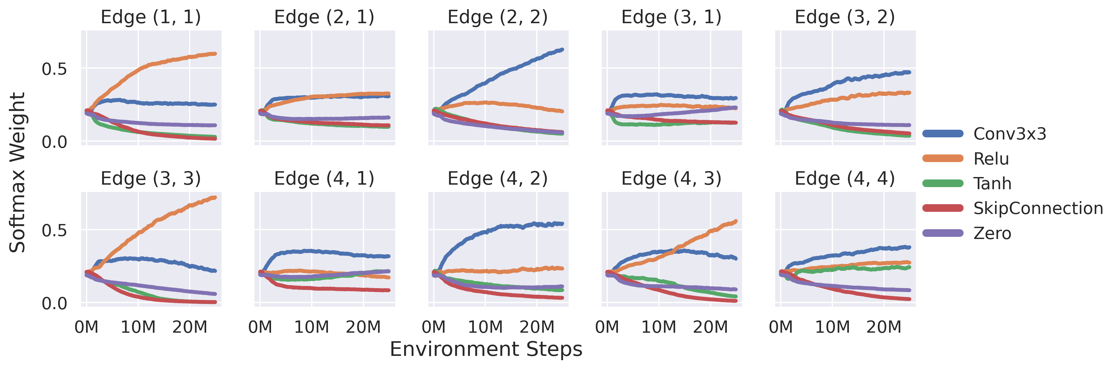
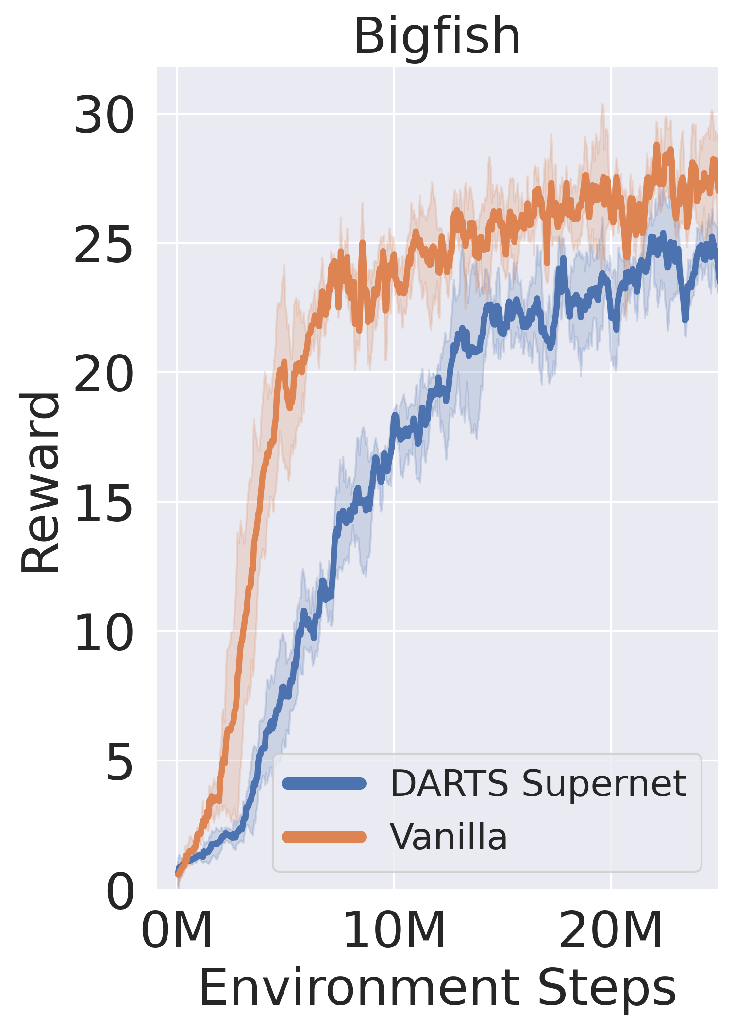
Figure 12: Analogous settings with Figure 8 using Rainbow + "Micro" search space. Left: Softmax weights when training Rainbow with infinite levels on Bigfish, also converging towards a sparser solution. Right: Sanity check for supernet when using Rainbow.

Appendix C What Affects Supernet Training?

Given the positive training results we demonstrated in the main body of the paper, one may wonder, can any supernet, no matter how poorly designed or setup, still train well in the RL setting? If so, this would imply that the search method would not be producing meaningful, but instead, random signals.

We refute this hypothesis by performing ablations over our supernet training in order to have a better understanding of what components affect its performance. We ultimately show that the search space and architecture variables play a very significant role in its optimization, thus validating our method.

C.1  Role of Search Space

We remove the ReLU nonlinearities from the "Classic" search space, so that $\mathcal{O}_{base}$ = $\{$Conv3x3, Conv5x5, Dilated3x3, Dilated5x5$\}$ and thus the DARTS cell consists of only linear operations. As shown in Fig. 13, this leads to a dramatic decrease in supernet performance, providing evidence that the search space matters greatly.

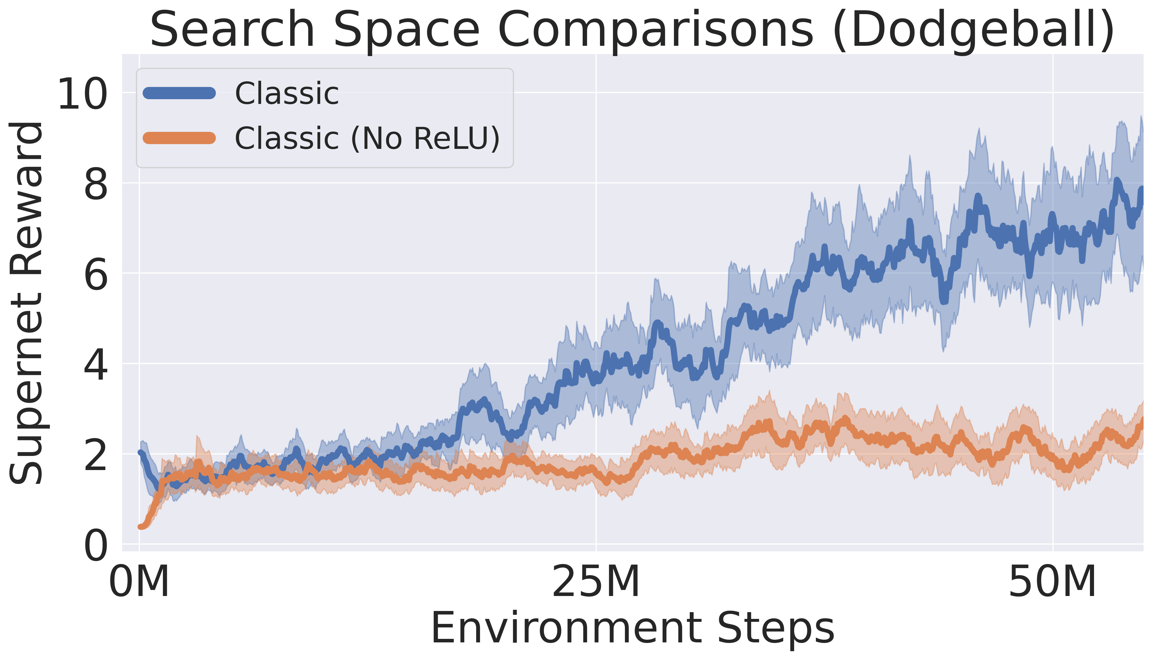
Figure 13: Supernet training using PPO on Dodgeball with infinite levels, when using the "Classic" search space with/without ReLU nonlinearities, under the same hyperparameters.

C.2  Uniform Architecture Variables

We further demonstrate the importance of the architecture variables $\alpha$ on training. We see that in Fig. 14, freezing $\alpha$ to be uniform throughout training makes the Rainbow agent unable to train at all. This suggests that it is crucial for $\alpha$ to properly route useful operations throughout the network.

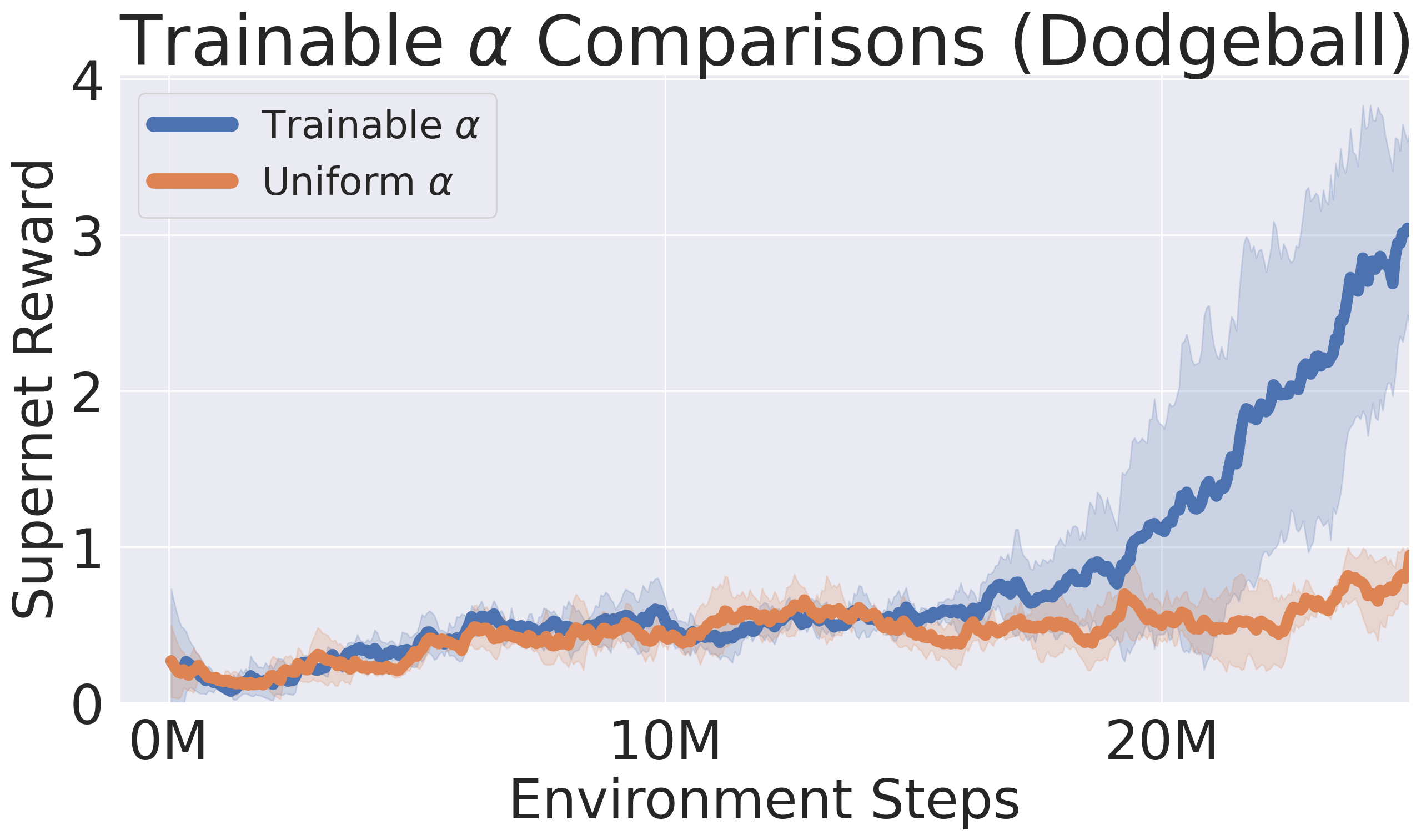
Figure 14: Supernet training using Rainbow on Dodgeball with infinite levels, when using the "Micro" search space with/without trainable architecture variables $\alpha$, under the same hyperparameters.

Appendix D What Affects Discrete Cell Performance?

D.1  Softmax Weights vs Discretization

As seen from Figure 8 in the main body of the paper, the DARTS supernet strongly downweights Conv5x5+ReLU operations when using the "Classic" search space with PPO. In order to verify the predictive power of the softmax weights, as a proxy, we thus also performed evaluations when using purely 3x3 or 5x5 convolutions on a large IMPALA-CNN with $64\times 5$ depths. We see that the Conv3x3 setting indeed outperforms Conv5x5, corroborating the results in which during training, $\alpha$ strongly upweights the Conv3x3+ReLU operation and downweights Conv5x5+ReLU.

D.2  Discrete Cell Evolutions

Along with Figure 10 in the main body of the paper, we also compare extra examples of discretizations before and after supernet training, to display reasonable behaviors induced by the trajectory of $\alpha$.

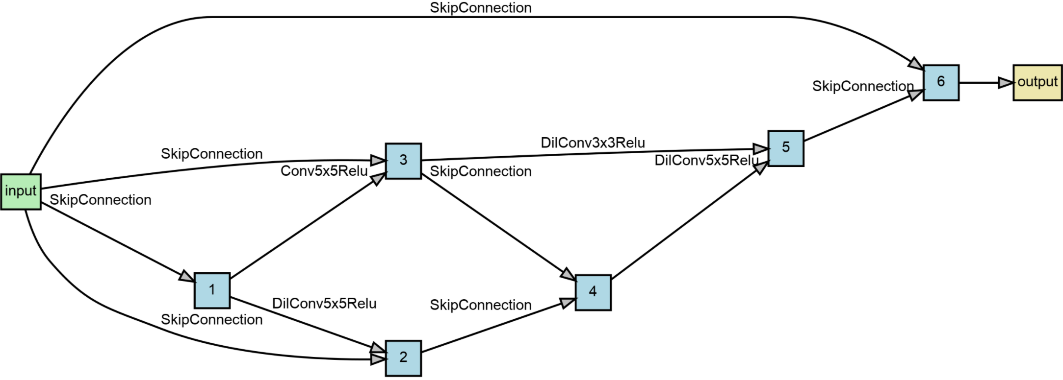
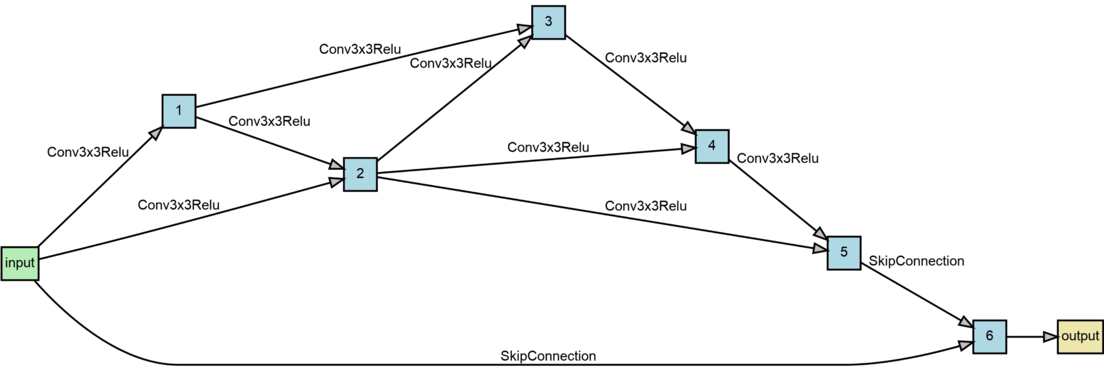
Figure 16: Comparison of discretized cells before and after supernet training, on Starpilot using PPO with $I=6$ nodes.

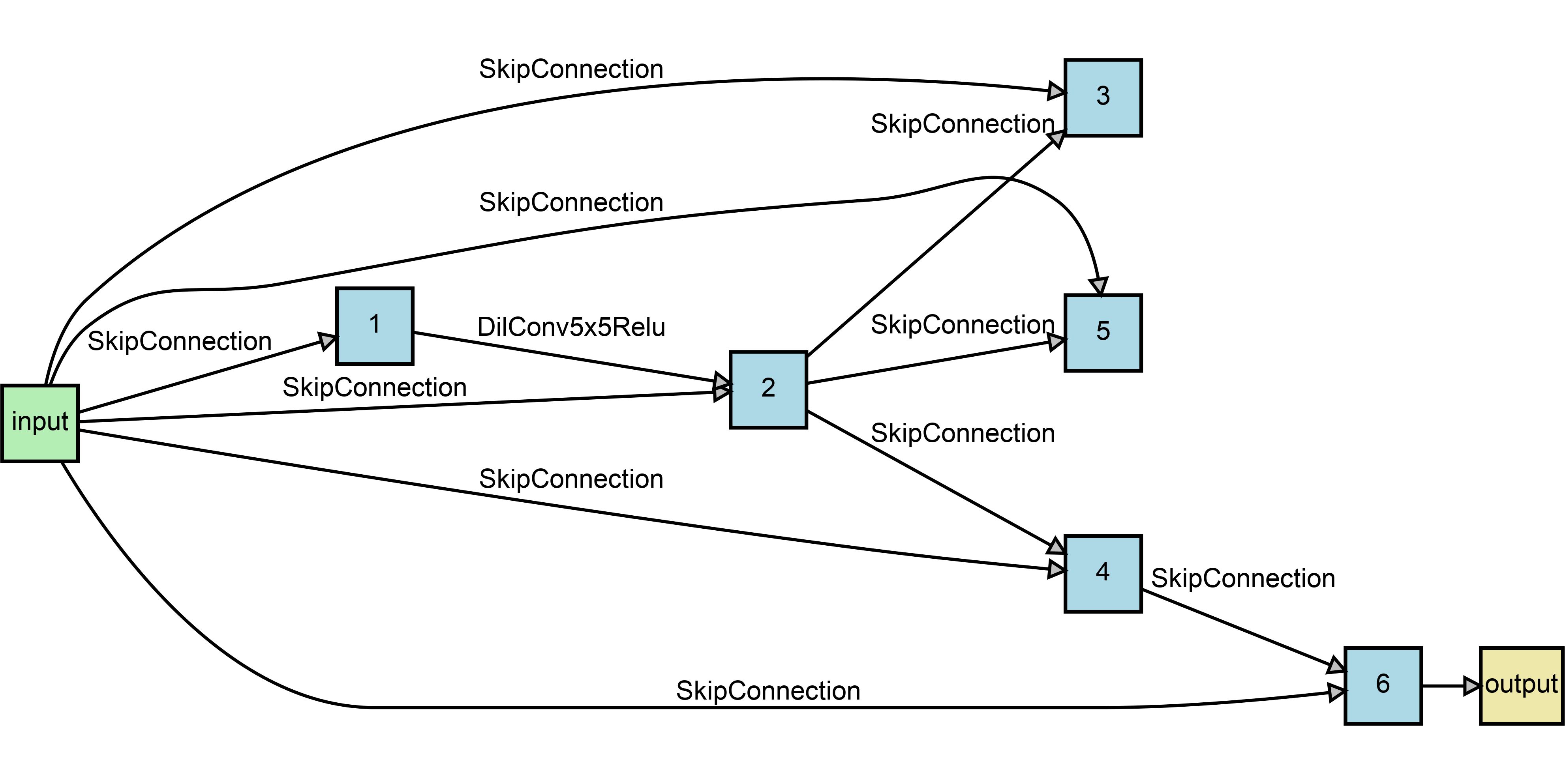
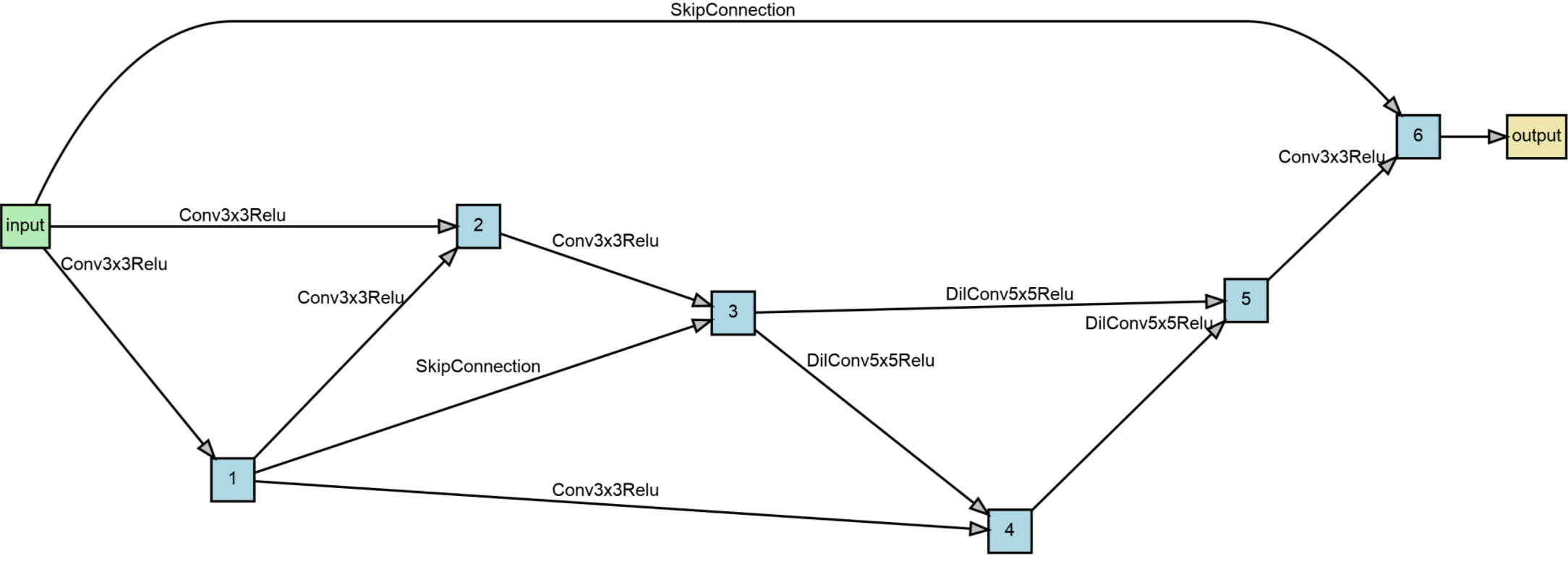
Figure 17: Comparison of discretized cells before and after supernet training, on Plunder using PPO with $I=6$ nodes.

In Figure 16, we use PPO with the "Classic" search space, but instead use $(N,R,I)=(1,0,6)$ along with outputting the last node (instead of concatenation with a Conv1x1 for the output) to allow a larger normal cell search space and graph topology. In Figure 17, the discretized cell initially uses a large number of skip connections as well as dead-end nodes. However, at convergence, it eventually utilizes all nodes to compute the final output. Curiously, we find that the skip connection between the input and output appears commonly throughout many searches.

For the Rainbow setting, in Figure 9 in the main body of the paper, we saw that when the search process is successful, the supernet’s training trajectory induces discretized cells which improve evaluation performance as well. The cells discovered later generally perform better than cells discovered earlier in the supernet training process. In Figure 18, we show more examples of such evaluation curves.

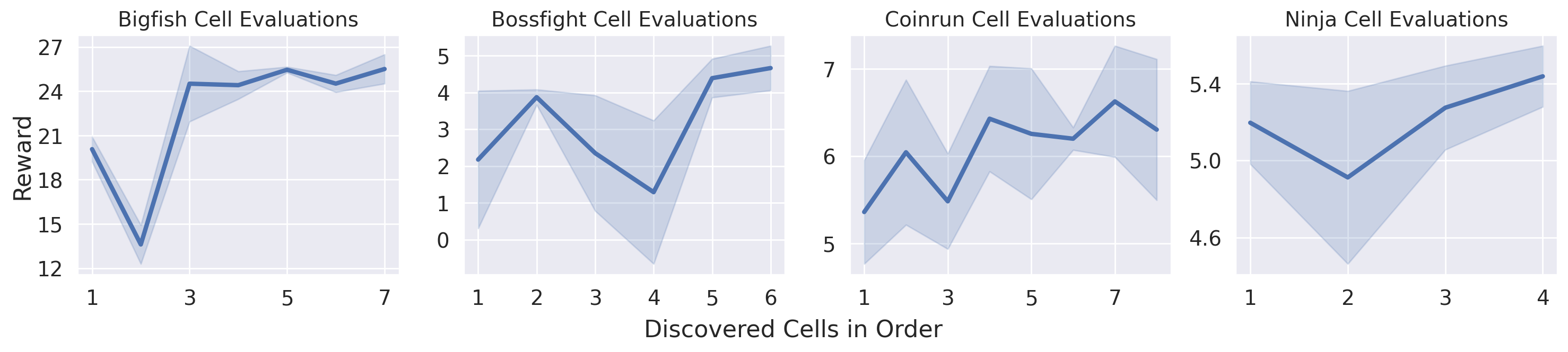
Figure 18: Evaluated discretized cells discovered throughout training the supernet with Rainbow. To save computation, we evaluate every 2nd cell that was discovered.

D.3  Correlation Between Supernet and Discretized Cells

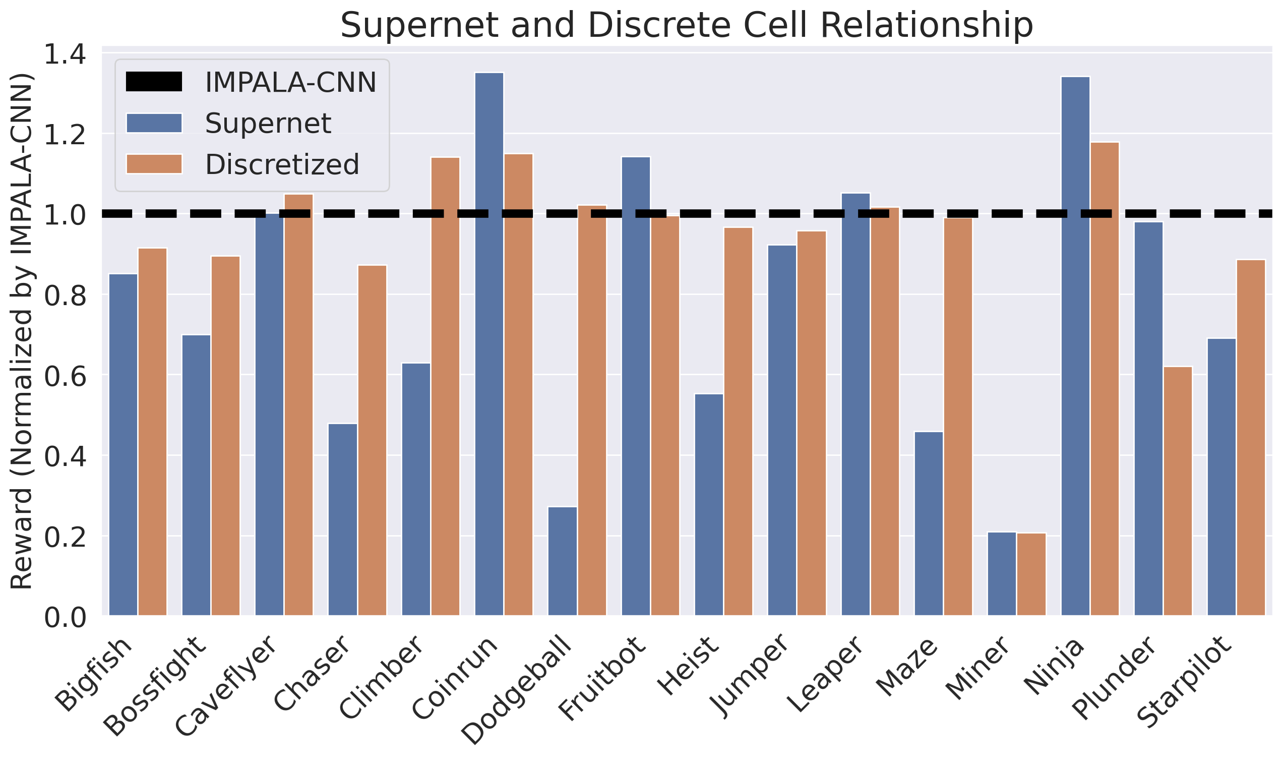
Figure 19: Supernet and their corresponding discrete cell rewards across all environments in Procgen using Rainbow, after normalizing using IMPALA-CNN’s performances. Thus, the black dashed line at 1.0 corresponds to IMPALA-CNN.

Given that the discretized cell only explicitly depends on architecture variables $\alpha$ and not necessarily model weights $\theta$, one may wonder: Is there a relationship between the rewards of the supernet and of its corresponding discretized cell? For instance, the degenerate/underperformance setting mentioned in Section 3.3 and Appendix D can be thought of as an extreme scenario. At the same time, there could be an integrality gap, where there the discretization process $\delta(\alpha)$ produces cells which give different rewards than the supernet.

In order to make such an analysis comparing rewards, we first must prevent confounding factors arising from Rainbow’s natural performance on an environment regardless of architecture. We thus first divide the supernet and discrete cell scores by the score obtained by the IMPALA-CNN baseline, where the baseline and discrete cells all used depths of $64\times 3$.

In Figure 19, when using Rainbow and observing across environments, we find both high correlation and also integrality gaps: for some environments such as Ninja and Coinrun, there is a significant correlation between supernet and discrete cell rewards, while for other environments such as Dodgeball, there is a significant gap. This suggests that search quality can be improved via both better supernet training such as using hyperparameter tuning or data augmentation (Raileanu et al.,, 2020), as well as better discretization procedures such as early stopping and stronger pruning (Chu et al., 2020a, ; Liang et al.,, 2019; Wang et al., 2021b, ).

Appendix E Numerical Scores

In Tables 5 and 20(b), we display the average normalized reward after 25M steps, as standard in Procgen (Cobbe et al.,, 2020), for a subset of environments in which RL-DARTS performs competitively. The normalized reward for each environment is computed as $R_{norm}=(R-R_{min})/(R_{max}-R_{min})$ where $R_{max}$ and $R_{min}$ are calculated using a combination of theoretical maximums and PPO-trained agents, and can be found in (Cobbe et al.,, 2020).

Env	IMPALA-CNN Baseline	RL-DARTS (Discrete)	Random Search
Bigfish	0.60	0.60	0.42
Bossfight	0.75	0.73	0.81
Caveflyer	0.75	0.47	0.85
Chaser	0.71	0.55	0.15
Climber	0.69	0.90	0.61
Coinrun	0.91	0.53	0.8
Dodgeball	0.53	0.59	0.29
Fruitbot	0.92	0.93	0.83
Heist	0.72	0.89	0.38
Jumper	0.62	0.76	1.0
Leaper	0.2	0.28	-0.28
Maze	1.0	1.0	0.0
Miner	0.74	0.85	0.70
Ninja	0.87	0.69	0.38
Plunder	0.57	0.76	0.43
Starpilot	0.71	0.73	0.40

(a)

Env	IMPALA-CNN Baseline	RL-DARTS (Discrete)	Random Search
Bigfish	0.71	0.65	0.60
Bossfight	0.54	0.48	0.45
Caveflyer	-0.05	-0.03	-0.01
Chaser	0.30	0.26	0.22
Climber	-0.04	-0.02	-0.05
Coinrun	0.06	0.21	0.15
Dodgeball	0.57	0.59	-0.05
Fruitbot	0.68	0.68	0.70
Heist	-0.48	-0.49	-0.47
Jumper	0.21	0.18	0.17
Leaper	-0.07	-0.07	-0.03
Maze	0.76	0.74	0.51
Miner	0.35	-0.03	0.11
Ninja	0.03	0.13	0.28
Plunder	0.14	0.02	0.03
Starpilot	0.91	0.80	0.76

(b)

Table 5: Normalized Rewards in ProcGen across different search methods, evaluated at 25M steps with depths $64\times 3$. Largest scores on the specific environment (as well as values within 0.03 of the largest) are bolded.

Appendix F Possible Improvements for Future Work

These include:

1. Discretization Changes: One may consider discretization based on the total reward $J(\pi_{\theta,\alpha})$, which may provide a better signal for the correct discrete architecture. This is due to the fact that the relative strengths of operation weights from $\alpha$ may not correspond to the best choices during discretization. (Wang et al., 2021b, ) considers iteratively pruning edges from the supernet based on maximizing validation accuracy changes. For RL, this would imply a variant of discretization dependent on multiple calculations of $J(\pi_{\theta^{*},\delta_{1}(\alpha^{*})})-J(\pi_{\theta^{*},\delta_{2}(\alpha^{*})})$ where $\theta^{*}$ consists the weights obtained during supernet training, as well as fine-tuning $J(\pi_{\theta^{*},\delta_{1}(\alpha^{*})})$ at every pruning step. These changes, in addition to the inherently noisy evaluations of $J(\cdot)$, greatly increase the complexity of the discretization procedure, but are worth exploring in future work.

2. Changing the Loss / Regularization: Throughout this paper, we have found that vanilla DARTS is able to train by simply optimizing $\alpha$ with respect to the loss, even though in principle, the loss is not strongly correlated to the actual reward in RL. Thus, it is curious to understand whether loss-based metrics or modifications may help improve RL-DARTS. One such modification is based on the observation that certain RL losses may not be required for training $\alpha$. In PPO, the entropy loss of $\pi_{\theta}$ may not be necessary or useful for improving the search quality of $\alpha$, and thus it may be better to perform a two step update by providing a different loss for $\alpha$. One may also consider searching for two separate encoders via two supernets, since both PPO and Rainbow feature separate networks, e.g. the policy $\pi_{\theta_{1},\alpha_{1}}$ and value function $V_{\theta_{2},\alpha_{2}}$ for PPO and advantage function $A_{\theta_{1},\alpha_{1}}$ and value function $V_{\theta_{2},\alpha_{2}}$ for Rainbow.

3. Signaling Metrics and Early Stopping: Observing metrics throughout training allows for early stopping, which can reduce search cost and provide better discrete cells. This includes metrics such as the strength of certain operation weights (Liang et al.,, 2019) as well as the Hessian with respect to $\alpha$ throughout training, i.e. $\nabla_{\alpha}^{2}\mathcal{L}(\theta,\alpha)$ as found in (Zela et al.,, 2020). Furthermore, inspired by performance prediction methods (Mellor et al.,, 2020; Luo et al.,, 2018), one may analyze metrics such as the Jacobian Covariance, via the score defined to be the $-\sum_{i=1}^{B}\left[\log(\sigma_{i}+\varepsilon)+(\sigma_{i}+\varepsilon)^{-1}\right]$ where $\varepsilon=10^{-5}$ is a stability constant and $\sigma_{1}\leq\ldots\leq\sigma_{B}$ are the eigenvalues of the correlation matrix corresponding to the Jacobian $J=\left[\frac{\partial f}{\partial s_{1}},\ldots,\frac{\partial f}{\partial s_{B}}\right]^{\top}$ with $B$ input images $\{s_{1},\ldots,s_{B}\}$.

   This metric/predictor has been found to be a strong signal for accuracy in SL NAS among many previous predictors (White et al.,, 2021). However, for the RL case, just like the loss, the mentioned metrics must be defined with respect to the current replay buffer $\mathcal{D}$, and thus raises the question of what type of data is to be used for calculating these metrics. When using a reasonable variant where the data is collected from a pretrained policy, we found that methods such as Jacobian Covariance did not provide meaningful feedback.

4. Supernet Training: As seen from the results in Figure 11 (main body) and Appendix D.3, there is a correlation between supernet and discrete cell performances. However, this is affected by the environment used as well as integrality gaps between the continuous relaxation and discrete counterparts, and thus further exploration is needed before concluding that improving the supernet training leads to better discrete cell performances. In any case, reasonable methods of improving the supernet can involve DARTS-agnostic modifications to the RL pipeline, including data augmentation (Kostrikov et al.,, 2020; Raileanu et al.,, 2020) as well as online hyperparameter tuning (Parker-Holder et al.,, 2020; Parker-Holder et al., 2021b, ). Simple hyperparameter tuning (e.g. on the softmax temperature for calculating $p_{o}^{(i,j)}$’s) also can be effective.

Appendix G Hyperparameters

In our code, we entirely use Tensorflow 2 for auto-differentation, as well as the April 2020 version of Procgen. For compute, we either used P100 or V100 GPUs based on convenience and availability. Below are the hyperparameter settings for specific methods. For all training curves, we use the common standard for reporting in RL (i.e. plotting mean and standard deviation across 3 seeds).

G.1  DARTS

Initially, we sweeped the softmax temperature in order to find a stable default value that could be used for all environments. For PPO, the sweep was across the set $\{1/5.0,1/10.0,1/15.0\}$. For Rainbow, the sweep was across $\{1/10.0,1/20.0,1/50.0\}$.

For tabular reported scores in Figures 5 and 20(b), we used a consistent softmax temperature of 1/5.0 for PPO, and 1/10.0 for Rainbow.

G.2  Rainbow-DQN

We use Acme (Hoffman et al.,, 2020) for our code infrastructure. We use a learning rate $5\times 10^{-5}$, batch size 256, n-step size 7, discount factor 0.99. For the priority replay buffer (Schaul et al.,, 2016), we use priority exponent 0.8, importance sampling exponent 0.2, replay buffer capacity 500K. For particular environments (Bigfish, Bossfight, Chaser, Dodgeball, Miner, Plunder, Starpilot), we use n-step size 2 and replay buffer capacity 10K. For C51 (Bellemare et al.,, 2017), we use 51 atoms, with $v_{min}=0,v_{max}=1.0$. As a preprocessing step, we normalize the environment rewards by dividing the raw rewards by the max possible rewards reported in (Cobbe et al.,, 2020).

G.3  PPO

We use TF-Agents (Guadarrama et al.,, 2018) for our code infrastructure, along with equivalent PPO hyperparameters found from (Cobbe et al.,, 2020). Due to necessary changes in minibatch size when applying DARTS modules or networks with higher GPU memory usage, we thus swept learning rate across $\{1\times 10^{-4},2.5\times 10^{-4},5\times 10^{-4}\}$ and number of epochs across $\{1,2,3\}$.

For all models, we use a maximum power of 2 minibatch size before encountering GPU out-of-memory issues on a standard 16 GB GPU. Thus, for a $16\times 3=[16,16,16]$ DARTS supernet, we set the minibatch size to be $256$, which is also used for evaluation with a $64\times 3=[64,64,64]$ discretized CNN. Our hyperparameter gridsearch for the evaluation led to an optimal setting of learning rate $=1\times 10^{-4}$ and number of epochs $=1$.

G.4  SAC

We use open-source code found in https://github.com/google-research/pisac, although we disabled the predictive information loss to use only regular SAC. The baseline architecture is a 4-layer convolutional architecture found in https://github.com/google-research/pisac/blob/master/pisac/encoders.py. Image-based observations are resized to $64\times 64$ with a frame-stacking of 3. Both our DARTS supernet and discrete cells use $N=3,I=4,K=1$ using the "Micro" search space, with convolutional depths of $32$ to remain fair to the baseline.

G.5  Training Procedure

Below are PPO (Schulman et al.,, 2017) and Rainbow-DQN (Hessel et al.,, 2018) RL-DARTS variants, which provide an example of the specific training procedure we use. Exact loss definitions and data collection procedures can be found in their respective papers.

Supernet training:

Setup supernet encoder $f_{\theta_{e},\alpha}$ with weights $\theta_{e}$.

Initialize policy and value head projection weights $W_{\pi}\in\mathbb{R}^{d,|\mathcal{A}|},W_{v}\in\mathbb{R}^{d,1}$.

Collect all trainable weights $\theta=\{\theta_{e},W_{\pi},W_{v}\}$.

Setup policy $\pi_{\theta,\alpha}(s)\sim\text{softmax}(W_{\pi}\cdot f_{\theta_{e},\alpha}(s))$.

Setup value function $V_{\theta,\alpha}(s)=W_{v}\cdot f_{\theta_{e},\alpha}(s)$.

Define standard PPO loss $\mathcal{L}(\theta,\alpha)$ using $\pi_{\theta,\alpha}$ and $V_{\theta,\alpha}$.

Perform PPO training via collecting data from $\pi_{\theta,\alpha}$ and SGD with $\nabla_{\theta,\alpha}\mathcal{L}(\theta,\alpha)$.

Collect $\alpha^{*}$ from previous training procedure.

Discretization:

Let $\delta(\alpha^{*})$ be the discrete cell constructed via Algorithm 4.

Evaluation:

Setup discretized cell encoder $f_{\phi_{e},\delta(\alpha^{*})}$.

Initialize policy and value head projection weights $W_{\pi}^{\prime}\in\mathbb{R}^{d,|\mathcal{A}|},W_{v}^{\prime}\in\mathbb{R}^{d,1}$.

Collect all trainable weights $\phi=\{\phi_{e},W_{\pi}^{\prime},W_{v}^{\prime}\}$.

Setup policy $\pi_{\phi,\delta(\alpha^{*})}(s)\sim\text{softmax}(W_{\pi}^{\prime}\cdot f_{\phi_{e},\delta(\alpha^{*})}(s))$.

Setup value function $V_{\phi,\delta(\alpha^{*})}(s)=W_{v}^{\prime}\cdot f_{\phi_{e},\delta(\alpha^{*})}(s)$.

Define standard PPO loss $\mathcal{L}_{\delta(\alpha^{*})}(\phi)$ using $\pi_{\phi,\delta(\alpha^{*})}$ and $V_{\phi,\delta(\alpha^{*})}$.

Perform PPO training via collecting data from $\pi_{\phi,\delta(\alpha^{*})}$ and SGD with $\nabla_{\phi}\mathcal{L}_{\delta(\alpha^{*})}(\phi)$.

Report final policy reward.

Algorithm 2 RL-DARTS with PPO

Supernet training:

Setup supernet encoder $f_{\theta_{e},\alpha}$ with weights $\theta_{e}$.

Initialize dueling network projections $W_{v}\in\mathbb{R}^{d,1},W_{a}\in\mathbb{R}^{d,|\mathcal{A}|}$.

Collect all trainable weights $\theta=\{\theta_{e},W_{v},W_{a}\}$.

Setup value network $V_{\theta,\alpha}(s)=W_{v}\cdot f_{\theta_{e},\alpha}(s)$.

Setup advantage network $A_{\theta,\alpha}(s,a)=W_{a}\cdot f_{\theta_{e},\alpha}(s)$.

Setup Q-network $Q_{\theta,\alpha}(s,a)=V_{\theta,\alpha}(s)+A_{\theta,\alpha}(s,a)-\frac{1}{|\mathcal{A}|}\sum_{a^{\prime}\in\mathcal{A}}A_{\theta,\alpha}(s,a^{\prime})$.

Define standard Rainbow loss $\mathcal{L}(\theta,\alpha)$ using $Q_{\theta,\alpha}$.

Perform Rainbow training via collecting data from $Q_{\theta,\alpha}$ and SGD with $\nabla_{\theta,\alpha}\mathcal{L}(\theta,\alpha)$.

Collect $\alpha^{*}$ from previous training procedure.

Discretization

Let $\delta(\alpha^{*})$ be the discrete cell constructed via Algorithm 4.

Evaluation

Setup discretized cell encoder $f_{\phi_{e},\delta(\alpha^{*})}$ with weights $\phi_{e}$.

Initialize dueling network projections $W_{v}^{\prime}\in\mathbb{R}^{d,1},W_{a}^{\prime}\in\mathbb{R}^{d,|\mathcal{A}|}$

Collect all trainable weights $\phi=\{\phi_{e},W_{v}^{\prime},W_{a}^{\prime}\}$

Setup value network $V_{\phi,\delta(\alpha^{*})}(s)=W_{v}^{\prime}\cdot f_{\phi_{e},\delta(\alpha^{*})}(s)$

Setup advantage network $A_{\phi,\delta(\alpha^{*})}(s,a)=W_{a}^{\prime}\cdot f_{\phi_{e},\delta(\alpha^{*})}(s)$

Setup Q-network $Q_{\phi,\delta(\alpha^{*})}(s,a)=V_{\phi,\delta(\alpha^{*})}(s)+A_{\phi,\delta(\alpha^{*})}(s,a)-\frac{1}{|\mathcal{A}|}\sum_{a^{\prime}\in\mathcal{A}}A_{\phi,\delta(\alpha^{*})}(s,a^{\prime})$

Define standard Rainbow loss $\mathcal{L}_{\delta(\alpha^{*})}(\phi)$ using $Q_{\phi,\delta(\alpha^{*})}$.

Perform Rainbow training via collecting data from $Q_{\phi,\delta(\alpha^{*})}$ and SGD with $\nabla_{\phi}\mathcal{L}_{\delta(\alpha^{*})}(\phi)$.

Report final policy reward.

Algorithm 3 RL-DARTS with Rainbow. Note that we do not use noisy nets in this implementation.

Argmax:

For $(i,j)$ across all edges:

Define edge strength $w_{i,j}=\max_{o\in\mathcal{O},o\neq zero}p_{o}^{(i,j)}$.

Define edge op $o_{(i,j)}=\operatorname*{arg\,max}_{o\in\mathcal{O},o\neq zero}p_{o}^{(i,j)}$.

Prune:

For node $j$ in all intermediate nodes:

Sort input edge weights $w_{i_{1},j}\geq w_{i_{2},j}\geq\ldots$

Retain only top $K$ edges $(i_{1},j),\ldots,(i_{K},j)$ and corresponding ops $o_{(i_{1},j)},\ldots,o_{(i_{K},j)}$ in final cell.

Algorithm 4 Discretization Procedure.

Note that both RL-DARTS procedures can also be summarized in terms of raw code as simple one-line edits to the image encoder used (compressing the rest of the regular RL training pipeline code):

def train(feature_encoder):
    """Initial RL algorithm setup"""
    ...
    extra_variables = Wrap(feature_encoder)
    all_trainable_variables =
       [feature_encoder.trainable_variables(), extra_variables]
    """Rest of RL algorithm setup"""
    ...
    apply_gradients(loss, all_trainable_variables)

Thus, the 3-step RL-DARTS procedure from Section 2 can be seen as:

DARTSSuperNet = MakeSuperNet(ops, num_nodes) # Setup
train(DARTSSuperNet) # Supernet training
DiscretizedNet = DARTSSuperNet.discretize() # Discretization
train(DiscretizedNet) # Evaluation

Appendix H Miscellaneous

H.1  Search Space Size

Let $O_{nz}=|\mathcal{O}|-1$, the number of non-zero ops in $\mathcal{O}$. For a cell (normal or reduction), the first intermediate node can only be connected to the input via a single op, and thus the choice is only $O_{nz}$. However, later intermediate nodes use $K=2$ inputs which leads to a choice size of $O_{nz}^{K}\times{i\choose K}$ where $i$ is the index of the intermediate node. Thus the total number of possible discrete cells is $O_{nz}\cdot\prod_{i=2}^{I}\left(O_{nz}^{K}\times{i\choose K}\right)$.

For the "Classic" search space, there are both normal and reduction cells to be optimized, with number of non-zero normal ops $O_{nz,N}=5$ and number of non-zero reduction ops $O_{nz,R}=4$, with $I=4,K=2$ for both. This leads to a total configuration size of $\left[O_{nz,N}\cdot\prod_{i=2}^{4}\left(O_{nz,N}^{2}\times{i\choose 2}\right)\right]\times\left[O_{nz,R}\cdot\prod_{i=2}^{4}\left(O_{nz,R}^{2}\times{i\choose 2}\right)\right]\approx 4\times 10^{11}$.

For the "Micro" search space, since we do not use reduction cells in order to simplify visualizations and ablation studies, $O_{nz,N}=4$ with $I=4,K=2$. This gives $\left[O_{nz,N}\cdot\prod_{i=2}^{4}\left(O_{nz}^{2}\times{i\choose 2}\right)\right]\approx 3\times 10^{5}$, which is comparable to the search space of size $5^{6}\approx 1.5\times 10^{4}$ in NASBENCH-201 (Dong and Yang,, 2020).

References

- Agarwal et al., (2010) Agarwal, A., Dekel, O., and Xiao, L. (2010). Optimal algorithms for online convex optimization with multi-point bandit feedback. In Kalai, A. T. and Mohri, M., editors, COLT 2010 - The 23rd Conference on Learning Theory, Haifa, Israel, June 27-29, 2010, pages 28–40. Omnipress.
- Akinola et al., (2021) Akinola, I., Angelova, A., Lu, Y., Chebotar, Y., Kalashnikov, D., Varley, J., Ibarz, J., and Ryoo, M. S. (2021). Visionary: Vision architecture discovery for robot learning. In ICRA.
- Bellemare et al., (2017) Bellemare, M. G., Dabney, W., and Munos, R. (2017). A distributional perspective on reinforcement learning. In Precup, D. and Teh, Y. W., editors, Proceedings of the 34th International Conference on Machine Learning, ICML 2017, Sydney, NSW, Australia, 6-11 August 2017, volume 70 of Proceedings of Machine Learning Research, pages 449–458. PMLR.
- Cai et al., (2019) Cai, H., Zhu, L., and Han, S. (2019). Proxylessnas: Direct neural architecture search on target task and hardware. In 7th International Conference on Learning Representations, ICLR 2019, New Orleans, LA, USA, May 6-9, 2019. OpenReview.net.
- Chen and Hsieh, (2020) Chen, X. and Hsieh, C. (2020). Stabilizing differentiable architecture search via perturbation-based regularization. In Proceedings of the 37th International Conference on Machine Learning, ICML 2020, 13-18 July 2020, Virtual Event, volume 119 of Proceedings of Machine Learning Research, pages 1554–1565. PMLR.
- (6) Chu, X., Wang, X., Zhang, B., Lu, S., Wei, X., and Yan, J. (2020a). DARTS-: robustly stepping out of performance collapse without indicators. CoRR, abs/2009.01027.
- (7) Chu, X., Zhang, B., and Li, X. (2020b). Noisy differentiable architecture search. CoRR, abs/2005.03566.
- (8) Chu, X., Zhou, T., Zhang, B., and Li, J. (2020c). Fair DARTS: eliminating unfair advantages in differentiable architecture search. In Vedaldi, A., Bischof, H., Brox, T., and Frahm, J., editors, Computer Vision - ECCV 2020 - 16th European Conference, Glasgow, UK, August 23-28, 2020, Proceedings, Part XV, volume 12360 of Lecture Notes in Computer Science, pages 465–480. Springer.
- Cobbe et al., (2020) Cobbe, K., Hesse, C., Hilton, J., and Schulman, J. (2020). Leveraging procedural generation to benchmark reinforcement learning. In Proceedings of the 37th International Conference on Machine Learning, ICML 2020, 13-18 July 2020, Virtual Event, volume 119 of Proceedings of Machine Learning Research, pages 2048–2056. PMLR.
- Cobbe et al., (2019) Cobbe, K., Klimov, O., Hesse, C., Kim, T., and Schulman, J. (2019). Quantifying generalization in reinforcement learning. In Chaudhuri, K. and Salakhutdinov, R., editors, Proceedings of the 36th International Conference on Machine Learning, ICML 2019, 9-15 June 2019, Long Beach, California, USA, volume 97 of Proceedings of Machine Learning Research, pages 1282–1289. PMLR.
- Dong and Yang, (2019) Dong, X. and Yang, Y. (2019). Searching for a robust neural architecture in four GPU hours. In IEEE Conference on Computer Vision and Pattern Recognition, CVPR 2019, Long Beach, CA, USA, June 16-20, 2019, pages 1761–1770. Computer Vision Foundation / IEEE.
- Dong and Yang, (2020) Dong, X. and Yang, Y. (2020). Nas-bench-201: Extending the scope of reproducible neural architecture search. In 8th International Conference on Learning Representations, ICLR 2020, Addis Ababa, Ethiopia, April 26-30, 2020. OpenReview.net.
- Duan et al., (2016) Duan, Y., Schulman, J., Chen, X., Bartlett, P. L., Sutskever, I., and Abbeel, P. (2016). Rl$^2$: Fast reinforcement learning via slow reinforcement learning. CoRR, abs/1611.02779.
- Espeholt et al., (2018) Espeholt, L., Soyer, H., Munos, R., Simonyan, K., Mnih, V., Ward, T., Doron, Y., Firoiu, V., Harley, T., Dunning, I., Legg, S., and Kavukcuoglu, K. (2018). IMPALA: scalable distributed deep-rl with importance weighted actor-learner architectures. In Dy, J. G. and Krause, A., editors, Proceedings of the 35th International Conference on Machine Learning, ICML 2018, Stockholmsmässan, Stockholm, Sweden, July 10-15, 2018, volume 80 of Proceedings of Machine Learning Research, pages 1406–1415. PMLR.
- Fortunato et al., (2019) Fortunato, M., Tan, M., Faulkner, R., Hansen, S., Badia, A. P., Buttimore, G., Deck, C., Leibo, J. Z., and Blundell, C. (2019). Generalization of reinforcement learners with working and episodic memory. In Wallach, H. M., Larochelle, H., Beygelzimer, A., d’Alché-Buc, F., Fox, E. B., and Garnett, R., editors, Advances in Neural Information Processing Systems 32: Annual Conference on Neural Information Processing Systems 2019, NeurIPS 2019, December 8-14, 2019, Vancouver, BC, Canada, pages 12448–12457.
- Gaier and Ha, (2019) Gaier, A. and Ha, D. (2019). Weight agnostic neural networks. In Wallach, H. M., Larochelle, H., Beygelzimer, A., d’Alché-Buc, F., Fox, E. B., and Garnett, R., editors, Advances in Neural Information Processing Systems 32: Annual Conference on Neural Information Processing Systems 2019, NeurIPS 2019, December 8-14, 2019, Vancouver, BC, Canada, pages 5365–5379.
- Guadarrama et al., (2018) Guadarrama, S., Korattikara, A., Ramirez, O., Castro, P., Holly, E., Fishman, S., Wang, K., Gonina, E., Wu, N., Kokiopoulou, E., Sbaiz, L., Smith, J., Bartók, G., Berent, J., Harris, C., Vanhoucke, V., and Brevdo, E. (2018). TF-Agents: A library for reinforcement learning in tensorflow. https://github.com/tensorflow/agents. [Online; accessed 21-May-2022].
- Haarnoja et al., (2018) Haarnoja, T., Zhou, A., Abbeel, P., and Levine, S. (2018). Soft actor-critic: Off-policy maximum entropy deep reinforcement learning with a stochastic actor. In Dy, J. G. and Krause, A., editors, Proceedings of the 35th International Conference on Machine Learning, ICML 2018, Stockholmsmässan, Stockholm, Sweden, July 10-15, 2018, volume 80 of Proceedings of Machine Learning Research, pages 1856–1865. PMLR.
- Hessel et al., (2018) Hessel, M., Modayil, J., van Hasselt, H., Schaul, T., Ostrovski, G., Dabney, W., Horgan, D., Piot, B., Azar, M. G., and Silver, D. (2018). Rainbow: Combining improvements in deep reinforcement learning. In McIlraith, S. A. and Weinberger, K. Q., editors, Proceedings of the Thirty-Second AAAI Conference on Artificial Intelligence, (AAAI-18), the 30th innovative Applications of Artificial Intelligence (IAAI-18), and the 8th AAAI Symposium on Educational Advances in Artificial Intelligence (EAAI-18), New Orleans, Louisiana, USA, February 2-7, 2018, pages 3215–3222. AAAI Press.
- Hoffman et al., (2020) Hoffman, M., Shahriari, B., Aslanides, J., Barth-Maron, G., Behbahani, F., Norman, T., Abdolmaleki, A., Cassirer, A., Yang, F., Baumli, K., Henderson, S., Novikov, A., Colmenarejo, S. G., Cabi, S., Gulcehre, C., Paine, T. L., Cowie, A., Wang, Z., Piot, B., and de Freitas, N. (2020). Acme: A research framework for distributed reinforcement learning. arXiv preprint arXiv:2006.00979.
- Hundt et al., (2019) Hundt, A., Jain, V., and Hager, G. D. (2019). sharpdarts: Faster and more accurate differentiable architecture search. CoRR, abs/1903.09900.
- James et al., (2019) James, S., Wohlhart, P., Kalakrishnan, M., Kalashnikov, D., Irpan, A., Ibarz, J., Levine, S., Hadsell, R., and Bousmalis, K. (2019). Sim-to-real via sim-to-sim: Data-efficient robotic grasping via randomized-to-canonical adaptation networks. In IEEE Conference on Computer Vision and Pattern Recognition, CVPR 2019, Long Beach, CA, USA, June 16-20, 2019, pages 12627–12637. Computer Vision Foundation / IEEE.
- Kalashnikov et al., (2018) Kalashnikov, D., Irpan, A., Pastor, P., Ibarz, J., Herzog, A., Jang, E., Quillen, D., Holly, E., Kalakrishnan, M., Vanhoucke, V., and Levine, S. (2018). Scalable deep reinforcement learning for vision-based robotic manipulation. In 2nd Annual Conference on Robot Learning, CoRL 2018, Zürich, Switzerland, 29-31 October 2018, Proceedings, volume 87 of Proceedings of Machine Learning Research, pages 651–673. PMLR.
- Kapturowski et al., (2019) Kapturowski, S., Ostrovski, G., Quan, J., Munos, R., and Dabney, W. (2019). Recurrent experience replay in distributed reinforcement learning. In 7th International Conference on Learning Representations, ICLR 2019, New Orleans, LA, USA, May 6-9, 2019. OpenReview.net.
- Kostrikov et al., (2020) Kostrikov, I., Yarats, D., and Fergus, R. (2020). Image augmentation is all you need: Regularizing deep reinforcement learning from pixels. CoRR, abs/2004.13649.
- Levine et al., (2020) Levine, S., Kumar, A., Tucker, G., and Fu, J. (2020). Offline reinforcement learning: Tutorial, review, and perspectives on open problems. CoRR, abs/2005.01643.
- Li et al., (2020) Li, G., Qian, G., Delgadillo, I. C., Müller, M., Thabet, A. K., and Ghanem, B. (2020). SGAS: sequential greedy architecture search. In 2020 IEEE/CVF Conference on Computer Vision and Pattern Recognition, CVPR 2020, Seattle, WA, USA, June 13-19, 2020, pages 1617–1627. IEEE.
- Li et al., (2021) Li, L., Khodak, M., Balcan, N., and Talwalkar, A. (2021). Geometry-aware gradient algorithms for neural architecture search. In 9th International Conference on Learning Representations, ICLR 2021, Virtual Event, Austria, May 3-7, 2021. OpenReview.net.
- Liang et al., (2019) Liang, H., Zhang, S., Sun, J., He, X., Huang, W., Zhuang, K., and Li, Z. (2019). DARTS+: improved differentiable architecture search with early stopping. CoRR, abs/1909.06035.
- Liu et al., (2018) Liu, C., Zoph, B., Neumann, M., Shlens, J., Hua, W., Li, L., Fei-Fei, L., Yuille, A. L., Huang, J., and Murphy, K. (2018). Progressive neural architecture search. In Ferrari, V., Hebert, M., Sminchisescu, C., and Weiss, Y., editors, Computer Vision - ECCV 2018 - 15th European Conference, Munich, Germany, September 8-14, 2018, Proceedings, Part I, volume 11205 of Lecture Notes in Computer Science, pages 19–35. Springer.
- Liu et al., (2019) Liu, H., Simonyan, K., and Yang, Y. (2019). DARTS: differentiable architecture search. In 7th International Conference on Learning Representations, ICLR 2019, New Orleans, LA, USA, May 6-9, 2019.
- Luo et al., (2018) Luo, R., Tian, F., Qin, T., Chen, E., and Liu, T. (2018). Neural architecture optimization. In Bengio, S., Wallach, H. M., Larochelle, H., Grauman, K., Cesa-Bianchi, N., and Garnett, R., editors, Advances in Neural Information Processing Systems 31: Annual Conference on Neural Information Processing Systems 2018, NeurIPS 2018, December 3-8, 2018, Montréal, Canada, pages 7827–7838.
- Mellor et al., (2020) Mellor, J., Turner, J., Storkey, A. J., and Crowley, E. J. (2020). Neural architecture search without training. CoRR, abs/2006.04647.
- Mnih et al., (2013) Mnih, V., Kavukcuoglu, K., Silver, D., Graves, A., Antonoglou, I., Wierstra, D., and Riedmiller, M. A. (2013). Playing atari with deep reinforcement learning. CoRR, abs/1312.5602.
- Nafi et al., (2021) Nafi, N. M., Glasscock, C., and Hsu, W. (2021). Attention-based partial decoupling of policy and value for generalization in reinforcement learning. In NeurIPS 2021 DeepRL Workshop.
- (36) Parker-Holder, J., Nguyen, V., Desai, S., and Roberts, S. J. (2021a). Tuning mixed input hyperparameters on the fly for efficient population based autorl. CoRR, abs/2106.15883.
- (37) Parker-Holder, J., Nguyen, V., Desai, S., and Roberts, S. J. (2021b). Tuning mixed input hyperparameters on the fly for efficient population based autorl. CoRR, abs/2106.15883.
- Parker-Holder et al., (2020) Parker-Holder, J., Nguyen, V., and Roberts, S. J. (2020). Provably efficient online hyperparameter optimization with population-based bandits. In Larochelle, H., Ranzato, M., Hadsell, R., Balcan, M., and Lin, H., editors, Advances in Neural Information Processing Systems 33: Annual Conference on Neural Information Processing Systems 2020, NeurIPS 2020, December 6-12, 2020, virtual.
- Parker-Holder et al., (2022) Parker-Holder, J., Rajan, R., Song, X., Biedenkapp, A., Miao, Y., Eimer, T., Zhang, B., Nguyen, V., Calandra, R., Faust, A., Hutter, F., and Lindauer, M. (2022). Automated reinforcement learning (autorl): A survey and open problems. CoRR, abs/2201.03916.
- Pham et al., (2018) Pham, H., Guan, M. Y., Zoph, B., Le, Q. V., and Dean, J. (2018). Efficient neural architecture search via parameter sharing. In Dy, J. G. and Krause, A., editors, Proceedings of the 35th International Conference on Machine Learning, ICML 2018, Stockholmsmässan, Stockholm, Sweden, July 10-15, 2018, volume 80 of Proceedings of Machine Learning Research, pages 4092–4101. PMLR.
- Pritzel et al., (2017) Pritzel, A., Uria, B., Srinivasan, S., Badia, A. P., Vinyals, O., Hassabis, D., Wierstra, D., and Blundell, C. (2017). Neural episodic control. In Precup, D. and Teh, Y. W., editors, Proceedings of the 34th International Conference on Machine Learning, ICML 2017, Sydney, NSW, Australia, 6-11 August 2017, volume 70 of Proceedings of Machine Learning Research, pages 2827–2836. PMLR.
- Raileanu and Fergus, (2021) Raileanu, R. and Fergus, R. (2021). Decoupling value and policy for generalization in reinforcement learning. In Meila, M. and Zhang, T., editors, Proceedings of the 38th International Conference on Machine Learning, ICML 2021, 18-24 July 2021, Virtual Event, volume 139 of Proceedings of Machine Learning Research, pages 8787–8798. PMLR.
- Raileanu et al., (2020) Raileanu, R., Goldstein, M., Yarats, D., Kostrikov, I., and Fergus, R. (2020). Automatic data augmentation for generalization in deep reinforcement learning. CoRR, abs/2006.12862.
- Rao et al., (2020) Rao, K., Harris, C., Irpan, A., Levine, S., Ibarz, J., and Khansari, M. (2020). Rl-cyclegan: Reinforcement learning aware simulation-to-real. In 2020 IEEE/CVF Conference on Computer Vision and Pattern Recognition, CVPR 2020, Seattle, WA, USA, June 13-19, 2020, pages 11154–11163. IEEE.
- Real et al., (2019) Real, E., Aggarwal, A., Huang, Y., and Le, Q. V. (2019). Regularized evolution for image classifier architecture search. In The Thirty-Third AAAI Conference on Artificial Intelligence, AAAI 2019, The Thirty-First Innovative Applications of Artificial Intelligence Conference, IAAI 2019, The Ninth AAAI Symposium on Educational Advances in Artificial Intelligence, EAAI 2019, Honolulu, Hawaii, USA, January 27 - February 1, 2019, pages 4780–4789. AAAI Press.
- Russakovsky et al., (2015) Russakovsky, O., Deng, J., Su, H., Krause, J., Satheesh, S., Ma, S., Huang, Z., Karpathy, A., Khosla, A., Bernstein, M. S., Berg, A. C., and Li, F. (2015). Imagenet large scale visual recognition challenge. Int. J. Comput. Vis., 115(3):211–252.
- Salimans et al., (2017) Salimans, T., Ho, J., Chen, X., and Sutskever, I. (2017). Evolution strategies as a scalable alternative to reinforcement learning. CoRR, abs/1703.03864.
- Schaul et al., (2016) Schaul, T., Quan, J., Antonoglou, I., and Silver, D. (2016). Prioritized experience replay. In Bengio, Y. and LeCun, Y., editors, 4th International Conference on Learning Representations, ICLR 2016, San Juan, Puerto Rico, May 2-4, 2016, Conference Track Proceedings.
- Schulman et al., (2017) Schulman, J., Wolski, F., Dhariwal, P., Radford, A., and Klimov, O. (2017). Proximal policy optimization algorithms. CoRR, abs/1707.06347.
- Song et al., (2021) Song, X., Choromanski, K., Parker-Holder, J., Tang, Y., Peng, D., Jain, D., Gao, W., Pacchiano, A., Sarlós, T., and Yang, Y. (2021). ES-ENAS: combining evolution strategies with neural architecture search at no extra cost for reinforcement learning. CoRR, abs/2101.07415.
- Song et al., (2020) Song, X., Jiang, Y., Tu, S., Du, Y., and Neyshabur, B. (2020). Observational overfitting in reinforcement learning. In 8th International Conference on Learning Representations, ICLR 2020, Addis Ababa, Ethiopia, April 26-30, 2020. OpenReview.net.
- Stanley et al., (2009) Stanley, K. O., D’Ambrosio, D. B., and Gauci, J. (2009). A hypercube-based encoding for evolving large-scale neural networks. Artif. Life, 15(2):185–212.
- Stanley and Miikkulainen, (2002) Stanley, K. O. and Miikkulainen, R. (2002). Efficient reinforcement learning through evolving neural network topologies. In Langdon, W. B., Cantú-Paz, E., Mathias, K. E., Roy, R., Davis, D., Poli, R., Balakrishnan, K., Honavar, V. G., Rudolph, G., Wegener, J., Bull, L., Potter, M. A., Schultz, A. C., Miller, J. F., Burke, E. K., and Jonoska, N., editors, GECCO 2002: Proceedings of the Genetic and Evolutionary Computation Conference, New York, USA, 9-13 July 2002, pages 569–577. Morgan Kaufmann.
- Tang and Ha, (2021) Tang, Y. and Ha, D. (2021). The sensory neuron as a transformer: Permutation-invariant neural networks for reinforcement learning. CoRR, abs/2109.02869.
- Tassa et al., (2018) Tassa, Y., Doron, Y., Muldal, A., Erez, T., Li, Y., de Las Casas, D., Budden, D., Abdolmaleki, A., Merel, J., Lefrancq, A., Lillicrap, T. P., and Riedmiller, M. A. (2018). Deepmind control suite. CoRR, abs/1801.00690.
- (56) Wang, H., Yang, R., Huang, D., and Wang, Y. (2021a). idarts: Improving DARTS by node normalization and decorrelation discretization. CoRR, abs/2108.11014.
- Wang et al., (2017) Wang, J., Kurth-Nelson, Z., Soyer, H., Leibo, J. Z., Tirumala, D., Munos, R., Blundell, C., Kumaran, D., and Botvinick, M. M. (2017). Learning to reinforcement learn. In Gunzelmann, G., Howes, A., Tenbrink, T., and Davelaar, E. J., editors, Proceedings of the 39th Annual Meeting of the Cognitive Science Society, CogSci 2017, London, UK, 16-29 July 2017. cognitivesciencesociety.org.
- (58) Wang, R., Cheng, M., Chen, X., Tang, X., and Hsieh, C.-J. (2021b). Rethinking architecture selection in differentiable nas. In International Conference on Learning Representations, ICLR 2021. OpenReview.net.
- White et al., (2021) White, C., Zela, A., Ru, B., Liu, Y., and Hutter, F. (2021). How powerful are performance predictors in neural architecture search? CoRR, abs/2104.01177.
- Zela et al., (2020) Zela, A., Elsken, T., Saikia, T., Marrakchi, Y., Brox, T., and Hutter, F. (2020). Understanding and robustifying differentiable architecture search. In 8th International Conference on Learning Representations, ICLR 2020, Addis Ababa, Ethiopia, April 26-30, 2020. OpenReview.net.
- Zhang et al., (2021) Zhang, B., Rajan, R., Pineda, L., Lambert, N. O., Biedenkapp, A., Chua, K., Hutter, F., and Calandra, R. (2021). On the importance of hyperparameter optimization for model-based reinforcement learning. CoRR, abs/2102.13651.
- Zoph and Le, (2016) Zoph, B. and Le, Q. V. (2016). Neural architecture search with reinforcement learning. CoRR, abs/1611.01578.
- Zoph et al., (2018) Zoph, B., Vasudevan, V., Shlens, J., and Le, Q. V. (2018). Learning transferable architectures for scalable image recognition. In 2018 IEEE Conference on Computer Vision and Pattern Recognition, CVPR 2018, Salt Lake City, UT, USA, June 18-22, 2018, pages 8697–8710. IEEE Computer Society.