A Kinematic Analysis of the Giant Molecular Complex W3; Possible Evidence for Cloud-Cloud Collisions that Triggered OB Star Clusters in W3 Main and W3(OH)

Abstract

The Hii region W3 is one of the most outstanding regions of high-mass star formation. Based on a new analysis of the ¹²CO($J$ = 2–1) data obtained at 38$\arcsec$ resolution, we have found that each of the two active regions of high-mass star formation, W3 Main and W3(OH), is associated with two clouds of different velocities separated by 3–4 km s^-1, having cloud mass of 2000–4000 $M_{\odot}$ in each. In the two regions we have found typical signatures of a cloud-cloud collision, i.e.,the complementary distribution with/without a displacement between the two clouds and/or a V-shape in the position-velocity diagram. We frame a hypothesis that a cloud-cloud collision triggered the high-mass star formation in the two regions. The collision in W3 Main involves a small cloud of $\sim$5 pc in diameter which collided with a large cloud of 10 pc $\times$ 20 pc. The collision in W3 Main compressed the gas in the direction of the collision path toward the west over a timescale of $\sim$1 Myr, where the dense gas W3 core associated with ten O stars are formed. The collision also produced a cavity in the large cloud having a size similar to the small cloud. The collision in W3(OH) has a younger timescale of $\sim$0.5 Myr and the forming-star candidates are heavily embedded in the clouds. The results reinforce the idea that a cloud-cloud collision is an essential process in high-mass star formation by rapidly creating the initial condition of 1 g cm^-2 in the natal gas.

1 Introduction

1.1 High-mass star formation

High-mass stars are important in our understanding of the galaxy evolution because their influence on the interstellar medium is substantial via ultraviolet radiations, stellar winds, and supernova explosions. Theoretical studies have shown that the initial gas conditions for star formation is a critical factor in order to realize the formation of high-mass stars (e.g., Zinnecker & Yorke, 2007). In particular, it has been argued that the mass density around 1 g cm^-2 is a necessary condition of high-mass stars formation as shown by the theoretical works (McKee & Tan, 2003; Krumholz et al., 2009). The high initial mass density most probably leads to a high mass accretion rate of 10^-4–$10^{-3}$ $M_{\odot}$ yr^-1, which is required to overcome the radiation pressure feedback by the forming high-mass stars (Wolfire & Cassinelli, 1987). Numerical simulations have shown that the competitive accretion model (Bonnell et al., 2003) or the monolithic collapse model (Krumholz et al., 2009) are possible mechanisms, whereas they are not readily compared with the observations. This is because the key signatures for confrontation are not always clearly pinpointed by the theoretical studies, allowing large room in interpretation of observations.

In the competitive accretion model, the initial condition is a massive cloud-star system of more than a few 1000 $M_{\odot}$ where individual stars compete to acquire mass gravitationally, whereas the model fails to explain the formation of an isolated small-mass system including isolated one or a few O stars which are distributed widely in the Galaxy (for a review see Fukui et al. 2021a; see also, Ascenso 2018). The monolithic collapse model assumes an initial condition “a massive gas cloud of 100 $M_{\odot}$ within a radius of 0.1 pc”, which matches the 1 g cm^-2 criterion, and it was numerically demonstrated that high-mass stars of 40 $M_{\odot}$ and 30 $M_{\odot}$ in a binary are formed (Krumholz et al., 2009). It remains however as an open question how such massive dense initial conditions are achieved in the interstellar space. It is required that the dense core has to be rapidly formed before the core is consumed by low-mass star formation prior to the formation of high-mass stars. It has been discussed also in the literature that high-mass stars are formed in massive hot cores or in the infrared dark clouds having very high column density (e.g., Egan et al., 1998). It is however a puzzle that they are always not associated with Hii regions which must be formed by O/early B stars, leaving room to doubt if they are really precursors of high-mass star formation (Tan et al., 2014). See also Motte et al. (2018) for a review on relevant observations.

Another line of approach to the issue is some sort of external triggering to compress gas and induce star formation in a cloud, which is called the “Triggered star formation” model. A classic model of such triggering is the gas compression by expanding Hii regions, often called the sequential star formation (Elmegreen & Lada, 1977). According to the model, if high mass stars are once formed, they compress the surrounding gas to a gravitationally unstable state which forms stars, and an age sequence of young OB stars in space can be realized which may explain the OB associations distributed observed roughly in age sequence (e.g., Lada et al., 1978). Another triggering mechanism is a cloud-cloud collision between two clouds with supersonic velocity separation. In the scheme, the gas is compressed in the interface layer between the clouds. These two models were first proposed by Oort and his collaborators in 1950–1960 (Oort & Spitzer, 1955; Oort, 1954). Based on optical spectroscopy of stars, Oort (1954) suggested collisions between the interstellar clouds taking place at 10–15 km s^-1 supersonic velocity. It was the first that Loren (1976) proposed a collision between two CO clouds triggered star formation in NGC 1333. Numerical simulations of a cloud-cloud collision by Habe & Ohta (1992), demonstrated that the collision between two clouds of different sizes may play a role in efficiently compressing the gas to trigger star formation, and were followed up by Anathpindika (2010), and Takahira et al. (2014). The study was further refined by including the magnetic field by Inoue & Fukui (2013), which showed that collisions are an effective process to trigger the formation of a high-mass cloud core, a precursor of high-mass star(s). Most recently, Fukui et al. (2021a) summarized the state of the art of the triggered star formation by cloud-cloud collisions based on around 50 candidate objects obtained by extensive CO surveys of high-mass star formation regions covering local star formation to the interacting galaxies which trigger massive clusters of $10^{6}$–$10^{7}$ $M_{\odot}$.

1.2 The W3 Giant Molecular Complex

W3 is a radio continuum source discovered by Westerhout (1958) and is a Hii region complex associated with a giant molecular complex (GMC) (for a review see Megeath et al., 2008). It is located in the Perseus Arm (e.g., Reid et al., 2016) and is continuous to another Hii region W4 along the Galactic Plane. In the boundary between W3 and W4 there is a high density layer (HDL) which is a molecular layer nearly vertical to the Galactic plane, nicely embracing W3. W3 is also known as a complex of particularly dense molecular gas condensations which harbours three distinct regions of active star formation named W3 Main, W3(OH), and AFGL 333 as shown by early CO observations (Lada et al., 1978). Between W3 Main and W3(OH) there is a diffuse Hii region IC 1795 (Mathys, 1989), and in the south of W3 Main a bright Hii region NGC 896 is located.

There are $\sim$100 OB stars in total in the W3 region. It is the most active site of star formation in the Perseus Arm (Ogura & Ishida, 1976; Oey et al., 2005; Navarete et al., 2011, 2019; Kiminki et al., 2015). These stars are divided into some clusters; the cluster associated with IC 1795 called W3 cluster (Navarete et al., 2019) and W3 Main and W3(OH) are also associated with clusters, respectively (e.g., Megeath et al., 2008). W3 Cluster is a most evolved cluster in W3 (Oey et al., 2005). OB stars in W3 Cluster have ages of 3–5 Myr according to the spectroscopic observations (Oey et al., 2005). The primary source of the ionization in W3 Cluster is BD+61 411, an O6.5V star (Oey et al., 2005). The Hii region IC 1795 has a circular shape ionized by W3 Cluster and a shell-like CO distribution is seen outside of it (Bieging & Peters, 2011), and W3 Main and W3(OH) appear to be associated with the shell.

W3 Main containing W3 West and W3 East shows in particular active star formation and its total mass is estimated to be 4000 $M_{\odot}$ (Bik et al., 2012). Cold pre-stellar cores and O stars as well as a hyper-compact Hii region and ultra-compact Hii regions are localized within a dimeter of $\sim$3 pc (Claussen et al., 1994; Tieftrunk et al., 1997; Bik et al., 2012; Mottram et al., 2020). The ongoing star formation is found also in W3 West and W3 East (e.g., Rivera-Ingraham et al., 2013). Especially, W3 West is known to harbour a Trapezium like cluster (Abt & Corbally, 2000; Megeath et al., 2005).

In W3(OH) region, OH masers and H₂O masers are localized within 0.1 pc (Forster et al., 1977; Reid et al., 1980). In addition, it is known that the OH maser is excited by an O9 star (Hirsch et al., 2012) and is associated with a ultra-compact Hii region of 0.012 pc diameter. Further, five early-type stars of B0–B3 are identified (Navarete et al., 2011; Bik et al., 2012; Kiminki et al., 2015; Navarete et al., 2019).

1.3 Star formation across the W3 Complex

The sequential star formation model (Elmegreen & Lada, 1977) has been discussed in W3 as a large-scale process of star formation. Lada et al. (1978) made a large-scale CO survey of the W3/W4/W5 region at 8$\arcmin$ resolution over 50 pc in the ¹²CO($J$ = 1–0) emission and proposed the sequential star formation. These authors discovered and mapped the HDL, and found that the HDL is forming stars younger than those in W4 by $\sim$10 Myrs, and suggested that the next generation stars were formed by trigger of the expansion of W4. Oey et al. (2005) made UBV photometry and derived age distribution of the stars in IC 1795. These authors proposed that the stars of 3–5 Myrs age in W3 Cluster were formed by the trigger of the Perseus/Chimney superbubble (Dennison et al., 1997) and that the star formation in W3 Main and W3(OH) was triggered by the expansion of IC 1795. The whole process was called “Hierarchical triggering”.

Recent higher-resolution observations at multi-wavelength however indicate that these simple pictures of sequential star formation may not work from distributions of stars and stellar ages. (Feigelson & Townsley, 2008) carried out an extensive study of stars of low-mass population with Chandra X-ray satellite in W3 Main, W3 Cluster and W3(OH). As a result, it was found that W3(OH) might have been formed by the stellar feedback from W3 Cluster. It is possible that the young stellar objects (YSOs) in W3 Main are distributed in a spherically symmetric manner, while star formation in W3(OH) can be formed by trigger of the feedback. These authors argued that the low-mass stars are not elongated in a shell shape and that it cannot be explained as due to the Hii expansion driven by W3 Cluster.

Bik et al. (2012, 2014) made infrared photometry by the LBT Near Infrared Spectroscopic Utility with Camera and Integral Field Unit for Extragalactic Research (LUCI, formerly LUCIFER) installed on the Large binocular telescope (LBT). As a result, these authors suggested that star formation in W3 Main began 2–3 Myr ago, and is continuing until now, causing a dispersion in age of a few Myr. It was also shown that the youngest stars lie in the central part of the cluster. Further, these authors suggested that feedback from the older stars in the W3 Main region does not propagate deeply into dense clouds probably due to higher initial gas density by more than 0.5 pc even after a few Myr after the cluster formation, not influencing thereby the cluster formation as a whole.

Román-Zúñiga et al. (2015) carried out an extensive study of the YSO age distribution through a JHK imaging by using the Calar Alto Observatory 3.5 m telescope for the objects in Chandra Source Catalog, Hershel SPIRE, PACS mosaics, and Bolocam 1.1 mm mosaic. These authors showed that there are many Class II sources in W3 Cluster in spite of that the molecular gas is largely dispersed already, and suggested that star formation has been very active until about 2 Myr ago. In addition, it was shown that W3 Main and W3(OH) include stellar population with the age of more than 2 Myr. Based on these, the authors concluded that in W3 Main and W3(OH) trigger by stellar feedback by IC 1795 cannot explain the age distribution.

These previous works presented doubts on the sequential star formation model, whereas they did not present an alternative global model on star formation. It therefore remains as an open issue how star formation took place across the W3 region.

1.4 The aim of the present paper

Star formation in W3 has not been fully understood yet in part due to the lack of a comprehensive study of the detailed gas kinematics. Recent studies extensively revealed the stellar properties in the region which include both high-mass and low-mass stars at sub-mm and X-rays as well as the deeply embedded stars. On the other hand, the molecular gas kinematics has not been investigated deeply in spite of that high resolution and wide-field mapping of CO and the other tracers become available in the last two decades. We therefore commenced a systematic study of the molecular gas obtained by Bieging & Peters (2011) with the Heinrich Hertz Sub-millimeter Telescope (HHT) which is employed using the analysis tools of gas kinematics developed in the last decade by Nagoya group on the molecular clouds (Fukui et al., 2021a): e.g., velocity channel distribution, position-velocity diagram, separation of individual clouds. In the study we aim to reveal a star formation mechanism which is dominant in W3 by utilizing the gas kinematic details and explore its implications on high-mass star formation. The AFGL 333 region was investigated by Nakano et al. (2017); Liang et al. (2021) and will not be dealt with in the present paper. This paper is organized as follows; Section 2 describes the datasets employed and Section 3 gives the results of the present kinematical analysis. In Section 4 we discuss the high mass star formation in W3 Main and W3(OH), and conclude the paper in Section 5.

2 Datasets

We used the $J$ = 2–1 line of ¹²CO and ¹³CO archived data observed with HHT at the Arizona radio observatory (Bieging & Peters, 2011). Observations were carried out in June, 2005 to April, 2008. They used the On-The-Fly (OTF) method to map a region of 200 times 167 square degrees. The map center was ($l$, $b$) = (13350, 0835). All the data were convolved to a spatial resolution of 38$\arcsec$. The velocity resolution is 1.30 km s^-1 at ¹²CO and 1.36 km s^-1 at ¹³CO, while they chose a sample velocity of 0.5 km s^-1. The typical root-mean-square (RMS) noise temperatures of the ¹²CO emission and ¹³CO emission are 0.12 K and 0.14 K, respectively. We preferred to use ¹²CO instead of ¹³CO in the present work because ¹²CO can better trace the low density extended molecular gas. This is crucial in identifying the cloud interaction, while it may be saturated in small dense regions.

3 Results

3.1 The overall distributions of the molecular gas

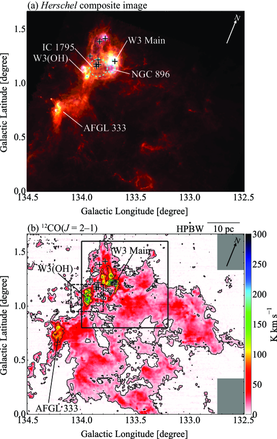
Figure 1: (a) Three-color composite image of the W3 GMC using Herschel PACS 70$~{}\mu$m (Blue), 160 $\mu$m (Green), and SPIRE 250 $\mu$m (Red). The colour tables have been manipulated to bring out the structural detail in the map. (b) Integrated intensity distribution of the ¹²CO($J$ = 2–1) emission for a velocity range from $-53$ km s^-1 to $-28$ km s^-1. The black boxes shown by the solid and dotted lines indicate the regions to be appeared in figures 4 and 10, respectively. Two rectangular regions filled in grey are not covered in the present data. The black crosses represent the positions of O-type stars detected by Oey et al. (2005). The lowest contour level and contour intervals correspond to 3 K km s^-1 and 60 K km s^-1, respectively.

Figure 1a shows the three colour image of Herschel taken with PACS at 70 $\mu$m, 160 $\mu$m, and SPIRE at 250 $\mu$m (Rivera-Ingraham et al. 2013). The whole W3 GMC is dominated by the red colour at 250 $\mu$m, while the area around ($l$, $b$)= (1337, 11) is bluer, indicating that dust components are heated by stellar feedback from high-mass stars.

Figure 1b shows the distribution of the integrated intensity of the ¹²CO($J$ = 2–1) emission which is extended by $\sim$60 pc $\times$ 60 pc. The O stars identified spectroscopically (Oey et al., 2005) are denoted by crosses. The diffuse gas is extended over the area and three regions in the northeast-east edge of the cloud show intense ¹²CO($J$ = 2–1) emission toward W3 Main, W3(OH), and AFGL 333 are described below. W3 Main has the most prominent peak at ($l$, $b$) = (13365, 120) with an integrated intensity of 450 K km s^-1. Most of the O stars are distributed within 10 pc of the peak position. W3(OH) at ($l$, $b$)$\sim$(1339, 11) has the integrated intensity 300 K km s^-1 and is associated with the OH and H₂O masers (Forster et al., 1977; Reid et al., 1980). A position of ($l$, $b$) = (1342, 07) weakest among the three is associated with W4 and is known as AFGL 333. The ultraviolet radiation of the O stars including BD+61 411 ionizes the surrounding gas to form an Hii region IC 1795 which is extended with a radius of $\sim$4 pc centered at ($l$, $b$) = (1337, 11) (Mathys, 1989). The area coincides with that of intense 70 $\mu$m emission in Figure 1a.

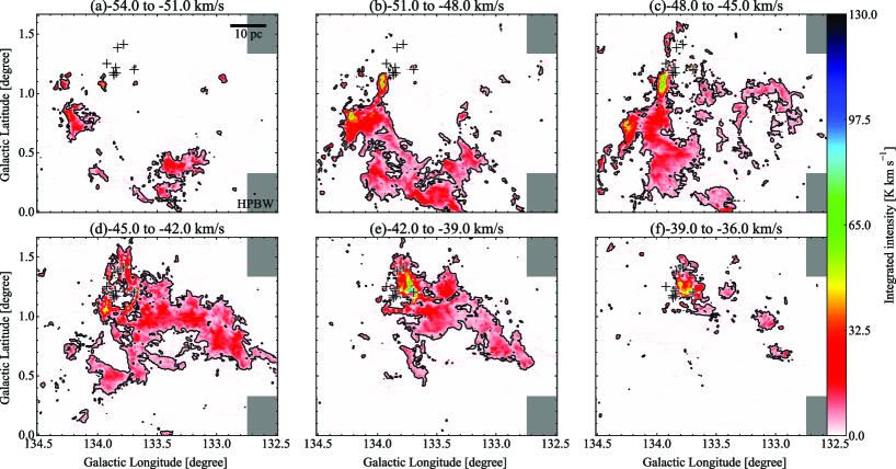
Figure 2: Velocity channel distribution of the ¹²CO($J$ = 2–1) line emission. Integration velocity ranges are denoted at the top of each panel. Superposed contour level is 2.6 K km s^-1. The black crosses represent the positions of O-type stars detected by Oey et al. (2005).

Figure 2 shows the velocity channel distributions of the W3 region. The distribution shows significant variation in velocity; the gas at $-55$–$-45$ km s^-1 is distributed in the southeastern part while the gas at $-45$–$-35$ km s^-1 is distributed in the northwestern part. The two velocity components seem to have different velocity ranges with the boundary at $-45$ km s^-1. The three peaks of the ¹²CO integrated intensity W3 Main, W3(OH), and AFGL 333 also show different velocity ranges at $-45$–$-35$ km s^-1, $-50$–$-40$ km s^-1, and $-55$–$-45$ km s^-1, respectively.

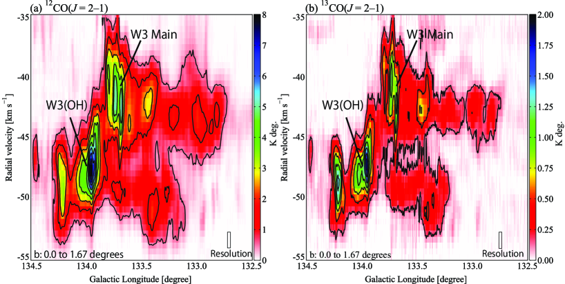
Figure 3: Galactic–longitude velocity diagram at (a) ¹²CO($J$ = 2–1) emission and (b) ¹³CO($J$ = 2–1) emission. The integration ranges are $b$=00 to 167. Contours are plotted every 1.0 K degree from 0.5 K degree ($\sim 16\sigma$) for ¹²CO($J$ = 2–1); every 0.3 K degree from 0.14 K degree ($\sim 7\sigma$) for ¹³CO($J$ = 2–1).

Figure 3 shows Galactic longitude-velocity diagrams of the W3 region. Figure 3a is for the ¹²CO($J$ = 2–1) emission and Figure 3b the ¹³CO($J$ = 2–1) emission. The two diagrams show similar distributions. In more, W3 Main and W3(OH) show velocity variations at a few pc scales. W3 Main shows velocity difference of 3–4 km s^-1 between at $l$ = 13365 and at $l$ = 13375, and W3(OH) shows a velocity shift of 4 km s^-1 at $l$ = 13385 from the peak position at $l$ = 13390. We shall focus on the two peaks in W3 Main and W3(OH) in the following and analyze their detailed distributions.

3.2 Gas properties in W3 Main

3.2.1 Gas distribution in W3 Main

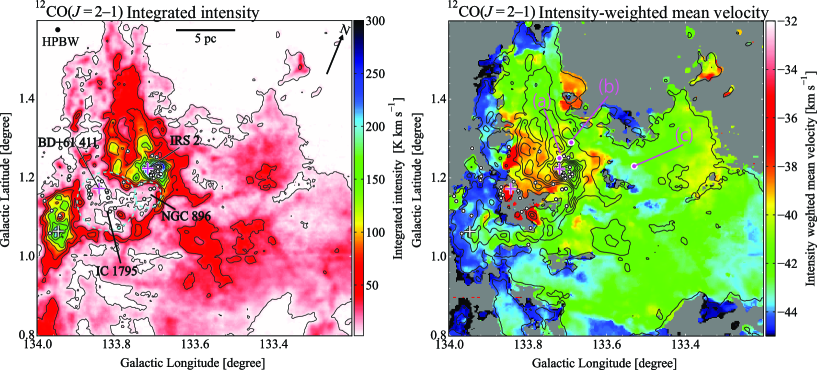
Figure 4: Left panel: Integrated intensity map of ¹²CO($J$ = 2–1) toward W3 Main. The integration velocity range is from $-53.0$ to $-35.0$ km s^-1. The black contours are plotted every 30 K km s^-1 from 5 K km s^-1. The white contours are plotted every 60 K km s^-1 from 278 K km s^-1. The cyan dotted circles represent distributions of the Hii regions IC 1795 and NGC 896. Right panel: Intensity-weighted mean velocity distributions of the ¹²CO($J$ = 2–1) emission. The calculation velocity range is from $-45.0$ to $-35.0$ km s^-1. Superposed contours show the integrated intensity distribution, same as Left panel. The magenta dots are the positions we present spectra in figure 5. The magenta crosses, white cross, and white dots indicate the positions of BD+61 411, IRS2, a driving source of the OH maser, and well-known OB stars (e.g., Navarete et al., 2019)

Figure 4 (left) shows the integrated intensity distribution of the W3 Main region, where the brightest peak corresponds to W3 Main, where $\sim 10$ O stars (white circles) including BD+61 411 are concentrated. The Hii regions IC 1795 and NGC 896 correspond to the cavity of the molecular gas. We see that the OB stars (Navarete et al., 2011, 2019; Bik et al., 2012) are distributed toward the center of IC 1795 and W3 Main. In the centre of IC 1795, the earliest-type star O6.5V in the region BD+61 411 is located and the most massive star IRS2 is associated with W3 Main (Bik et al., 2012). The molecular cavity coincides with these Hii regions, whereas BD+61 411 is offseted from the centre of the Hii region shell.

Figure 4 (right) shows the distribution of the first moment for a velocity range of $-45.0$–$-35.0$ km s^-1. Only the voxels with intensity greater than $6\times T_{\mathrm{rms}}=0.72$ K are included. The velocity range of W3(OH) is not included, and is dealt with later in section 3.3. Most of the emission is in a velocity range from $-45.5$ to $-42.5$ km s^-1, whereas red-shifted emission is seen in a range from to $-40.5$ to $-37.0$ km s^-1 with a size of $\sim$5 pc in the east of W3 Main.

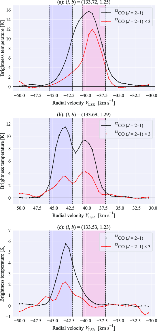
Figure 5: ¹²CO($J$ = 2–1) and ¹³CO($J$ = 2–1) spectra at the positions (a) to (c) in figure 4 (right). The blue and the red ribbons represent the velocity range of the W3 Main blue cloud and the W3 Main red cloud.

Figure 5 shows typical CO spectra in the W3 Main region. We confirm the trend of Figure 4 in these spectra with peaks at $-40.5$ to $-37.0$ km s^-1 and $-45.5$ to $-42.5$ km s^-1; Figure 5a at ($l$, $b$) = (13372, 125) and Figure 5c at ($l$, $b$) = (13353, 123) show peaks which have about $\sim$5 km s^-1 velocity difference. Figure 5b at ($l$, $b$) = (13353, 123) shows a double peak, which is apparent both in ¹²CO and ¹³CO, indicating that it is not likely due to self-absorption because the ¹³CO emission is optically thin. We hereafter refer a cloud at a velocity range of $-40.5$ km s^-1 to $-37.0$ km s^-1 cloud as W3 Main red cloud and at $-45.5$ km s^-1 to $-42.0$ km s^-1 cloud as W3 Main blue cloud.

3.2.2 The red- and blue-shifted gas in W3 Main

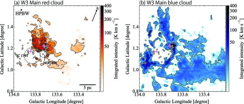
Figure 6: (a) Integrated intensity distribution of the W3 Main red cloud. The integration range is from $-40.5$ km s^-1 to $-37.0$ km s^-1. The lowest and the intervals of the superposed contours are 11.7 K km s^-1 and 15 K km s^-1, respectively. (b) Integrated intensity distribution of the W3 Main blue cloud. The integration velocity range is from $-45.5$ km s^-1 to $-42.0$ km s^-1. The lowest and the intervals of the superposed contours are 8 K km s^-1 and 30 K km s^-1, respectively. The magenta crosses, white cross, and white dots indicate the positions of BD+61 411, IRS2, a driving source of the OH maser, and well-known OB stars (e.g., Navarete et al., 2019).

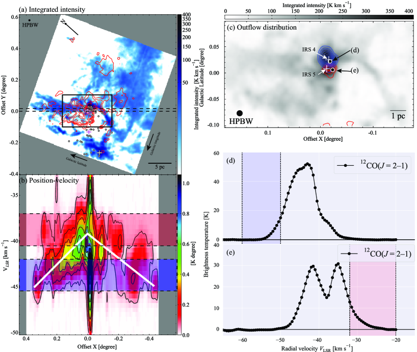
Figure 7: (a) ¹²CO($J$ = 2–1) integrated intensity distribution of the W3 Main red cloud and W3 Main blue cloud in the offset X–Y coordinates. The coordinate is defined by rotating the galactic coordinate counterclockwise by 7000. The integration velocity range is from $-45.5$ km s^-1 to $-42.0$ km s^-1 for the colour image; $-40.5$ K km s^-1 to $-37.0$ K km s^-1 for the contours. The lowest and the intervals of superposed the contours are 11.7 K km s^-1 and 15 K km s^-1. The black box indicates the region to be appeared in (c). The magenta crosses, white cross, and white dots indicate the positions of BD+61 411, IRS2, a driving source of the OH maser, and well-known OB stars (e.g., Navarete et al., 2019) (b) Offset Y–velocity diagram of the W3 Main region in ¹²CO($J$ = 2–1). Integration range along the Offset Y is donated as dotted lines in (a). The velocity ranges of each cloud are represented by red and blue transparent belt. The lowest level and the interval of the superposed contours are 0.08 K degree and 0.20 K degree. White line indicate a V-shape. (c): Integrated intensity distribution of the red wing and the blue wing are indicated by the red and the blue contours, respectively. The lowest level of the red and the blue contours are 10 K km s^-1 and 5 K km s^-1 , respectively. The intervals of red and the blue contours are 7 K km s^-1 and 5 K km s^-1 respectively. Image shows the intensity integrated for a velocity range of $-53$ km s^-1 to $-35$ km s^-1. (d): Typical spectral profile at position (d) in (c). (e): Typical spectral profile at position (e) in (c). The red and the blue ribbons indicate the velocity range of the red- and the blue-shifted wing.

Figures 6a and 6b show the W3 Main red and blue clouds, respectively. We see that W3 Main red cloud is compact and its shape fits approximately the cavity of the blue cloud. Figure 7a shows the distribution of the two clouds which are rotated by 70 degrees counterclockwise relative to the Galactic plane centred on IRS2, and Figure 7b a position-velocity diagram along the horizontal axis in Figure 7a. We find significant line-broadening toward the peak of W3 Main. At offset X$\sim$0.0, indicating molecular outflow lobes as mentioned by previous studies (e.g., Román-Zúñiga et al., 2015). Figure 7c shows the distributions of red- and blue-shifted lobes, where extended outflowing wings are also seen in the spectral profiles in Figures 7d and 7e. Note that the red- and blue-lobes are driven by multiple sources associated with the infrared point sources IRS4 and IRS5 (Wang et al., 2013; Mottram et al., 2020). In the present beam the two outflow lobes are not fully resolved, and hence it is not discussed further in this paper. By excluding the wings we find a V-shape as illustrated by the white line in Figure 7b.

3.3 Gas properties in W3(OH)

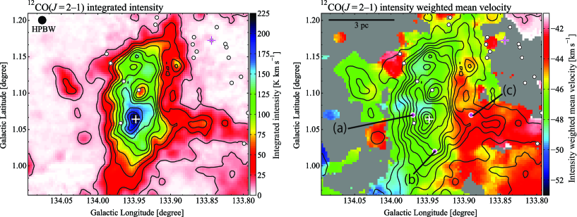
Figure 8: Left panel: Integrated intensity distribution of the W3(OH) region. Integration range is from $-53$ K km s^-1 to $-41.0$ K km s^-1. The lowest and the interval of the overlaid contours are 10 K km s^-1 and 12 K km s^-1, respectively. Right panel: Intensity weighted mean velocity distribution of the W3(OH) region. The calculation range and overlaid contours are the same as (a). Magenta dots (a) to (c) indicate the position we present spectrum in figure 11. The magenta cross, white cross, and white dots represent the location of of BD+61 411, a driving source of the OH maser, and well-known OB stars (e.g., Navarete et al., 2019).

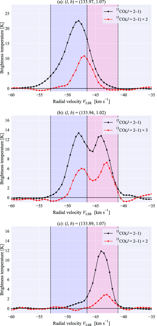
Figure 9: ¹²CO($J$ = 2–1) and ¹³CO($J$ = 2–1) spectra at the positions (a) to (c) in figure 8 (right). The blue and the red ribbons represents the velocity range of the W3(OH) blue cloud and the W3(OH) red cloud.

Figure 8 (left) shows the integrated intensity distribution of ¹²CO($J$ = 2–1) in the W3(OH) region. The molecular emission peak at ($l$, $b$) = (13395, 107) is associated with an OH maser (Forster et al., 1977; Reid et al., 1980). There are three O stars within a pc of ($l$, $b$) = (13385, 116). Figure 8 (right) shows the distribution of the first moment. We find that the central velocity is different by $\sim$5 km s^-1 between the high $l$ part and low $l$ part at a boundary $l$ = 13391. Figure 9a shows a profile at ($l$, $b$) = (13397, 107), and represents a typical profile having $-48$ km s^-1 at the high $l$ part of $l$ = 13391. Figure 9c shows that having $-42$ km s^-1 at ($l$, $b$) = (13389, 107) and represents a typical one in the low $l$ part of $l$ = 13391. Figure 9b shows a double peaked profile between the two positions. Because the double peak is seen both in ¹²CO and ¹³CO, it is not due to self-absorption in ¹²CO. In summary, we infer that there are two velocity components and denote the $-46.5$ to $-41.0$ km s^-1 gas the W3(OH) red cloud, and the $-53.0$ to $-46.5$ km s^-1 cloud the W3(OH) blue cloud.

3.4 The physical parameters of the molecular clouds

We derived column densities and masses of the molecular clouds under an assumption of the local thermodynamic equilibrium. First, we assumed the ¹²CO($J$ = 2–1) line is optically thick, and obtained excitation temperatures in every pixel. Then, we calculated an optical depth of the ¹³CO($J$ = 2–1) line, and derived the column densities. Next, we obtained column densities assuming an abundance ratio of the ¹³CO molecules and the H₂ molecules of $7.1\times 10^{5}$ (Frerking et al., 1982). Finally, we got the masses of the clouds from the derived column densities. We note that a summation of the red cloud and the blue cloud in W3(OH) is somewhat larger than the total cloud because the excitation temperatures are calculated in each cloud. The physical parameters are summarized in Table 1. For details of the analyses, see Appendixes. We also confirm that column densities derived in the present study are consistent with those derived from Herschel observations with a factor of 2 to 3 (Rivera-Ingraham et al., 2013).

4 Discussion

W3 Cluster has ages of 3–5 Myr and the Hii region is disrupting the parental molecular clouds. The disruption makes it difficult to grasp details of the gas kinematics and the cluster formation mechanism on a large scale. On the other hand, the O stars in W3 Main and W3(OH) have ages less than 2 Myr and star formation is supposed to be on-going in the molecular gas, which may help us to elucidate the star formation mechanism through a detailed analysis of the molecular gas. We discuss the high mass star formation in the W3 Main and W3(OH) regions based on the present CO results.

4.1 Trigger of star formation by the expansion of the Hii region

The scenario of sequential star formation driven by OB associations was proposed and discussed by Elmegreen & Lada (1977). In the W3 region, Lada et al. (1978) presented a model that the W4 Hii region expanded to compress the gas to form the HDL in the W3 region which led to trigger star formation. Subsequently, Oey et al. (2005) proposed a “Hierarchical triggering” model where the expansion of the Perseus chimney/super bubble in W4 triggered the formation of W3 Cluster and the feedback of W3 Cluster triggered the active star formation in W3 Main and W3(OH). These previous studies are based on the stellar-age distribution, whereas detailed kinematics and distribution of the parental molecular gas were not analysed/considered in depth. We aim to better understand the star formation by using the velocity and density distribution of the CO molecular gas.

We find two molecular clouds in the W3 Main region (Section 3). The two clouds have velocity difference of $\sim$4 km s^-1, and a usual explanation for the velocity difference is gas acceleration by the high-mass stars. In the present case, a possible scenario is that the momentum released by W3 Cluster is responsible for the acceleration of the W3 Main red cloud relative to W3 Main blue cloud. Because W3 Main red cloud seems to be accelerated by $\sim$4 km s^-1 from the systemic velocity if we regard the V-shape structure in the position velocity diagram as a red-shifted half of the expanding shell (see figure 7b). Further, W3 Main red cloud has an elongated structure toward BD+61 411, which may correspond to a blown-off cloud efficiently overtaken by the stellar wind (e.g., Fukui et al., 2017; Sano et al., 2018). To evaluate the expansion scenario, We first consider the stellar winds as the momentum source. The highest mass star in W3 Cluster is an O6.5V star BD+61 411 (Oey et al., 2005). The momentum delivered by the star to the surroundings in a time span of 3–5 Myr, the age of the cluster (Oey et al., 2005), is expressed as follows;

$$P_{\mathrm{winds}}=\dot{M}v\cdot\Delta t$$ (1)

where $P_{\mathrm{winds}}$ is the wind momentum, $\dot{M}$ the mass loss rate, and $\Delta t$ the cluster age. The typical wind mass loss rate of an O6.5V star is $10^{-6.4}$ $M_{\odot}$ yr^-1 (Vink et al., 2000) and its terminal velocity is 2600 km s^-1 (Kudritzki & Puls, 2000). If we assume that W3 Cluster contains ten O6.5V star, we estimate $P_{\mathrm{winds}}=3.1\times 10^{4}$ km s^-1 $M_{\odot}$. The momentum required to accelerate a cloud of $M_{\mathrm{cloud}}$ to a relative velocity $V_{\mathrm{rel}}$ is given as follows if a complete coupling of the momentum to the cloud mass is assumed;

$$P_{\mathrm{clouds}}=\dot{M}_{\mathrm{clouds}}V_{\mathrm{rel}}$$ (2)

By taking the cloud mass accelerated by 4 km s^-1 to be 8100 $M_{\odot}$, we obtain $P_{\mathrm{cloud}}=3.24\times 10^{4}$ km s^-1 $M_{\odot}$. This value is comparable to that of supplied by the stellar winds. Importantly, we further need to consider the realistic geometry of the clouds and the stars. The solid angle subtended by the cloud relative to W3 Cluster seem to be significantly less than 4$\pi$ due to the inhomogeneous distribution of the clouds as shown by the weak CO emission toward W3 Cluster (Figure 6a). This indicates that the stellar feedback is hardly able to explain the cause of the velocity difference.

It has been a usual thought over a long time that the Hii regions can accelerate and compress the surrounding gas. This possibility was studied theoretically by Kahn (1954) and it was shown that there is a solution corresponding to the acceleration phase of the neutral gas driven by the Hii gas under a range of two parameters, the stellar ultraviolet photons and the gas density. By hydrodynamical numerical simulations without magnetic field, Hosokawa & Inutsuka (2005) showed that the gas around an O star is accelerated and compressed leading to star formation. Subsequently, Krumholz et al. (2007) made 3D magnetohydrodynamical numerical simulations of the interaction between an Hii region and magnetized neutral gas. they showed that the Hii region expands in a direction parallel to the magnetic field lines, whereas the expansion is strongly suppressed in the direction perpendicular to the field lines by the magnetic pressure. They concluded thus that the triggered star formation is much less effective than thought previously without magnetic field. It is also known that the Champagne flow makes the Hii gas escape from a low density part of the surrounding gas (Tenorio-Tagle, 1979; see Figure 4 in Megeath et al., 2008), leading to even less compression. W3 seems to be one of such a case. In summary, recent numerical studies of the interaction of a Hii region with the ambient neutral gas show that a Hii region may not play a role in gas compression.

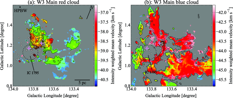
Figure 10: a) Intensity weighted mean velocity distribution of the W3 Main red cloud. (b) Intensity weighted mean velocity distribution of the W3 Main blue cloud. The contours in the two panels are the same as figure 6. The magenta crosses, white cross, and white dots indicate the positions of BD+61 411, IRS2, a driving source of the OH maser, and well-known OB stars (e.g., Navarete et al., 2019).

We are in fact able to see a trend of no acceleration of molecular gas in the present data. Figure 10 shows the first moment distributions of the W3 Main red cloud and the W3 Main blue cloud. W3 Main blue cloud in Figure 10b shows that there is no appreciable velocity shift of the molecular gas facing the Hii region at the present resolution, which contradicts the previous numerical simulations without magnetic field predicting a velocity shift (see Figure 1 of Hosokawa & Inutsuka, 2005). The W3 Main blue cloud has shell-like distribution and has first moment at $-43$ km/s over the whole extent with insignificant velocity variation. This may suggest that, while the cloud has a shell morphology, feedback by the W3 Cluster has a small effect on the overall cloud kinematics/distribution. On the other hand, W3 Main red cloud shows small velocity variation less than $\sim$1.5 km s^-1 in some places. Part of it may be due to the feedback of the stars, while the effect does not seem to be prevailing. We note that small scale triggering star formation at “sub-pc scale” has been discussed in the previous works (Tieftrunk et al., 1997; Wang et al., 2013; Rivera-Ingraham et al., 2013), while we do not deal with them further in the present work of pc-scale resolution.

In summary, it seems that the usual scenario of feedback by high-mass stars is not able to explain the present observations of the W3 molecular gas in triggering star formation. This is along the line which has been argued for in the recent works, whereas the trigger process by stellar feedback in star formation has not yet been fully tested yet including the effects of small scale clumps.

4.2 An alternative scenario; Cloud-cloud collisions

We discussed it unlikely that the sequential star formation model was able to explain the star formation in W3 Main and W3(OH). In this section, we test a scenario based on cloud-cloud collisions (CCCs), which are suggested to be operating in the other typical young Hii regions including the Orion region, the Carina region, and the M16 and M17 region (Fukui et al., 2021a, 2018; Enokiya et al., 2021b; Fujita et al., 2021; Nishimura et al., 2018, 2021) and we examine a CCC scenario as an alternative to Hii-triggered star formation in W3 Main and W3(OH).

Fukui et al. (2021a) summarized the main observational signatures of a CCC, where two clouds with a supersonic velocity separation associated with a young star/cluster or their candidates as follows;

1. complementary spatial distribution between the two clouds, and

2. bridge feature(s) connecting the two clouds in velocity space, and

3. U shaped morphology.

Numerical simulations of a CCC were employed in deriving these signatures, while the three signatures may not be always found in a CCC object depending on the cloud dispersal by the stellar ionization and/or feedback etc. Further, the hydrodynamical numerical simulations show additional features including a projected displacement between the two clouds when the collision direction is not parallel to the line of sight (Habe & Ohta, 1992; Anathpindika, 2010; Takahira et al., 2014; Haworth et al., 2015). Such complementary distributions with a displacement are observed in synthetic observations of the numerical simulation data as well as observations of molecular gas e.g., in M42 etc. (Fukui et al., 2018). Further, in position-velocity diagrams CCC sometimes appears as a V-shape in a position-velocity diagram, or bridge features connecting two clouds (see M43 in Fukui et al., 2018), where an intermediate velocity component is formed via the momentum exchange between the two clouds (e.g., Takahira et al., 2014; Haworth et al., 2015). A typical case of the U-shaped cavity is found in the numerical simulations by Habe & Ohta (1992) and is observed in RCW 120 etc. (See Figure 5 of Fukui et al., 2021a).

In W3 Main we argue that the properties of the W3 Main red cloud and the W3 Main blue cloud show the three observed signatures i-iii) of CCC. $\sim$4 km s^-1, a projected velocity separation, gives a lower limit to the actual collision velocity, and is larger than the typical linewidth of the two clouds. A realistic local sound speed is given by the Alfvenic speed which is a few km/s if density and magnetic field are assumed to be 300 cm^-3 and $20$ $\mathrm{\mu}$G, respectively (Inoue & Fukui, 2013). The two clouds are peaked toward IRS2 in the cluster identified by (Bik et al., 2012), which corresponds to the densest part in the U-shaped morphology, and match the picture of a U-shape.

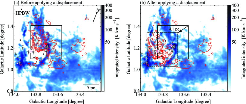
Figure 11: Complementary ¹²CO($J$ = 2–1) distributions of the W3 Main red cloud and W3 Main blue cloud. The integration velocity range is from $-45.5$ km s^-1 to $-42.0$ km s^-1 for the color image; $-40.5$ km s^-1 to $-37.0$ km s^-1 for the contours. The lowest and the intervals of superposed the contours are 11.7 K km s^-1 and 15 K km s^-1. The colour image and the contour indicates the W3 Main red cloud and the W3 Main blue cloud, respectively. The magenta crosses, white cross, and white dots indicate the positions of BD+61 411, IRS2, a driving source of the OH maser, and well-known OB stars (e.g., Navarete et al., 2019).

Figure 11a shows an overlay of the W3 Main blue cloud and the W3 Main red cloud. The W3 Main Blue cloud is extended beyond the outside of W3 Main as diffuse emission, while the W3 Main red cloud has a clear boundary of a 5-pc diameter. In order to test if a cloud-cloud collision is a possible scenario, we applied the algorithm of the displacement by Fujita et al. (2021). This code optimises the correlation coefficient between the W3 Main red shifted clouds and the W3 Main blue shifted cloud enclosed by the two boxes in Figure 10a. We then obtained the best correlation coefficient of $-0.53$, which is appropriate to fit a displacement (e.g., Fujita et al., 2021; Sano et al., 2021). We found that a displacement of 4.1 pc to the south achieves a good matching with the cavity in the large cloud. Figure 7 shows a V-shape in the position velocity diagram as indicated by the white line superposed. The W3 Main red cloud is more compact than the W3 Main blue cloud, the top of the V-shape is extended more toward the W3 Main red cloud.

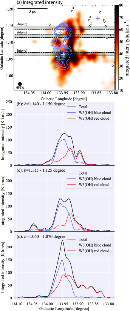
Figure 12: (a) ¹²CO($J$ = 2–1) distributions of the W3(OH) red cloud and the W3(OH) blue cloud. The integration velocity range is from $-53.0$ km s^-1 to $-46.5$ km s^-1 for the colour image; $-46.5$ km s^-1 to $-41.0$ km s^-1 for the contours. The lowest and the intervals of the superposed contours are 60 K km s^-1 and 10 K km s^-1. (b–d) Integrated intensities of each cloud averaged along the galactic latitude. Positions of each profile are indicated as dark transparent belts enclosed by the dotted lines in (a). The magenta crosses, white cross, and white dots indicate the positions of BD+61 411, a driving source of the OH maser, and well-known OB stars (e.g., Navarete et al., 2019).

We suggest that the W3(OH) region also is explicable by a CCC scenario. This region has two velocity components at $-44$ km s^-1 and $-48$ km s^-1 and is associated with an OH maser source and a H₂O maser source as well as a few B stars. Figure 12a shows a complementary distribution between the two clouds. Figures 12b–12d show a strip map of Figure 12a, which presents the integrated intensity in the dark shaded area averaged in Galactic Latitude. The Blue, Red, and black lines show W3(OH) blue cloud, W3(OH) red cloud, the whole W3(OH) cloud, respectively. We find that the W3(OH) blue cloud and the W3(OH) red cloud are overlapping with each other at $l$ = 13390–13395, and suggest it possible that the two clouds are merging via collision there.

The W3(OH) region is separated from the W3 Main by $\sim$300 pc, which is much large than their apparent separation of about $\sim$10 pc, in the sky according to the recent GAIA DR2 distance (Navarete et al., 2019), and we may consider the two regions are independent from each other in spite of their apparent closeness in the sky.

4.3 A possible CCC scenario

Based on the signatures in Section 4.2. we assume that CCCs are operating in the W3 Main and W3(OH) regions and discuss the high mass star formation there.

4.3.1 The W3 Main region

We propose a hypothesis that the W3 Main red cloud and the W3 Main blue cloud collided with each other and are compressing the gas toward IRS2 to trigger the star formation in the dense gas. The collision is likely continuing until now. We use the displacement in Figure 11b in order to estimate the time scale of the collision. By assuming the collision direction has an angle of 45 degrees to the line of sight tentatively, the timescale is estimated to be 4.1 pc / 4 km s^-1$\sim$1.0 Myr. The timescale varies by the angle between the collision direction and the line of sight and, if we assume 60 and 30 degrees, the time scales become 0.6 Myr and 1.8 Myr, respectively. We therefore assume that the collision time scale is in a range of 0.6–1.8 Myr. This is consistent with the stellar age of $\sim$1–2 Myr (Bik et al., 2012, 2014). We note that an angle of the projection is not likely close to 0 or 90 degrees as inferred from the large displacement and the significant relative velocity.

The direction of the displacement with a position angle of $\sim$300 degrees with respect to the Galactic North pole suggests that the W3 Main red cloud is moving toward the direction over the last 1–2 Myr. We find that the collision picture is consistent with the matching between the W3 Main red cloud cloud and the molecular cavity when the displacement is applied. Furthermore, we note that the location of W3 Main almost coincides with the direction connecting W3 Main and the centre of the cavity at ($l$,$b$) = (1338, 11), and this configuration is consistent with what the Habe & Ohta (1992) predicts in a CCC.

The present analysis does not cover the direction of IC 1795 where the CO gas is mostly ionised, and does not constrain the star formation there in the same way as in W3 Main. Nonetheless, it seems possible that the collision in its initial phase triggered the formation of IC 1795 in a duration of 0.1 Myr about 1–2 Myr ago. Following the formation of IC 1795, the W3 Main red cloud continued the collision to accumulate the mass which is observed as W3 Main now, if the picture is correct.

Rivera-Ingraham et al. (2013) used the Herschel dust temperature and showed that the eastern clump of the two dense clumps (W3 East, W3 West) associated with W3 Main as temperature above 30 K, the western show 25 K , These authors argued that in W3 East dust is heated by the high mass stars including IRS5 including Trapezium-system and by IRS2, 0.5 pc to the north. On the other hand, W3 West has no high mass stars formed yet kept lower dust temperature. Román-Zúñiga et al. (2015) suggested that in W3 Main class I/0 to class II ratio is enhanced toward the direction where star formation is propagating to the collision direction. This suggests that star formation is propagating to the direction. These previous studies presented a trend consistent with the present CCC scenario. W3 Main red cloud is moving to the north along with the compressed layer. Habe & Ohta (1992) showed that collision between two clouds star are formed in the compressed layer and with the motion of the layer, star formation propagates to the north. Note that the proper motion of the forming stars reflect more localized gas motion in a small scale and does not always agree with the motion vector (e.g., Inoue et al., 2018).

Next, we estimate Star Formation Efficiency (SFE) in W3 Main. The total cluster mass in W3 Main is about 4000 $M_{\odot}$ (Bik et al., 2012). According to figure 4, there is a molecular gas condensation at 0.5 pc west of IRS2, and about 10 O stars are concentrated. The peak integrated intensity of the condensation is 493 K km s^-1. We draw a contour line at an integrated intensity of 110 K km s^-1, corresponding to $\sim$22$\%$ of the peak integrated intensity and defined the enclosed area as W3 core. The total molecular mass in W3 core is 3400 $M_{\odot}$ and we obtain SFE = (Cluster mass) / (Cluster mass $+$ Molecular mass) = 54$\%$, which is slightly higher than that of the typical value of CCC objects according to Fukui et al. (2021b).

In summary, our scenario of the CCC is that the W3 Red cloud having a smaller size collided with the extended W3 Blue cloud to create a cavity in the Blue cloud. The initiation of the collision dates back to 1–2 Myr ago and the W3 Red cloud likely triggered star formation continuously over 1–2 Myr, which has a potential to explain the formation of IC 1795 and NGC 896 having an age spanning from 0.1 Myr to 2 Myr (e.g., Bik et al., 2012), whereas the ionization by IC 1795 dispersed their parental clouds, making it impossible to witness the associated molecular gas.

This scenario proposes that a collision between two molecular clouds is triggering star formation in a 5 pc scale continuously in W3 Main. in addition, the feedback from the W3 Cluster is not likely trigger star formation in W3 Main. Whereas a small scale trigger by the Hii region may still be taking place locally (e.g., Rivera-Ingraham et al., 2013). A CCC can form dense clumps of a few pc and locally the feedback may be working. To be emphasized is that the formation of the dense gas at W3 Main and stars of age spread of $\sim$2 Myrs can be explained by the current model but not by the stellar feedback from W3 Cluster.

4.3.2 The W3(OH) region

Star formation in W3(OH) seems to be less active and in an earlier stage than in W3 Main as suggested by a few OB stars and the embedded OH maser within the two clouds at different velocities (Figure 8b, 9). The two clouds in apparent contact raise a possibility of a cloud-cloud collision in W3(OH), which we shall examine in the following.

Figure 12 shows that W3(OH) red cloud has a size of $\sim$3 pc in the Galactic latitude, whose extent is similar to that of the bright part above 60 K km s^-1 of the W3(OH) blue cloud. Figure 9 shows that the typical velocities of W3(OH) blue cloud and W3(OH) red cloud are -48 km s^-1 and -43 km s^-1, respectively, with typical linewidths of $\sim$4 km s^-1. We find that the two clouds show considerable overlapping in projection, which is most significant toward the OH maser source, and that the red cloud shows an extension of $\sim$3 pc toward the west at latitude of 1.06 degrees nearly the latitude of the OH maser. The CO results indicate complementary distribution of the two clouds, a typical signature of colliding clouds and we suggest that a cloud-cloud collision is a possible interpretation of the two clouds. The small separation of the two clouds in velocity $\sim$5 km s^-1 relative to their linewidths $\sim$4 km s^-1 explains no bridge feature between the two. A possible scenario is as follows; the two clouds are colliding with each other at a projected velocity of $\sim$5 km s^-1. The collision timescale is roughly estimated to be 0.2 Myr by a ratio of the typical cloud width $\sim$ 1.5 pc, the apparent separation of the CO peak of W3(OH) blue cloud from the edge of W3(OH) red cloud, and the relative velocity $\sim$7.1 km s^-1 by assuming that the collision velocity makes an angle of 45 degrees to the line of sight. In the scenario, the blue cloud is moving to the west and the collision is on its half way. The timescale varies from 0.14 to 0.25 Myr with an assumed angle of 30-60 degrees. The blue cloud is not yet interacting with the western part of the red cloud, which is consistent with the westward extension of the red cloud. The collisional merging seems to be most intense toward the maser source.

4.4 Comparison with the other CCC candidates

It is known that W3 Main has a Trapezium-like cluster (Abt & Corbally, 2000). Table 2 compares the two clusters and indicates that the star formation in W3 Main share similar molecular column density and age to the Orion Nebula Cluster (ONC) (For a review , see Muench et al., 2008 and references therein).

In the ONC, Fukui et al. (2018) identified two clouds with velocity difference of $\sim$4 km s^-1 which are shown to have complementary distribution which is consistent with a CCC triggered the OB stars in the ONC. These authors presented a scenario that the ONC consists of two populations one was formed by the CCC in the last 0.1 Myr and the other low mass members which are being continuously formed over the last 1.5 Myr.

SFE in W3 core was estimated to be $\sim$54$\%$, while SFE in the ONC was estimated to be $\sim$20$\%$ (e.g., Fukui et al., 2021a). This deference may be due to the presence of OB stars having older age in W3 Main. UV photons and stellar wind from OB stars disrupt molecular gas, which may enhance SFE. Fukui et al. (2021b) showed that SFE is not particularily enhanced in a compressed layer of CCC, and a few $\%$ to a few times 10$\%$ are typical values. This suggestion is also consistent with the present result when we consider the larger stellar ages.

The present study revealed that W3 shows evidence for triggered high-mass star formation by CCCs, where sufficiently high column density gas with $\sim$10²³ cm^-2 is colliding. Enokiya et al. (2021a) compiled 50 CCC candidates and made a statistical study, and have shown that the number of O and early B stars are correlated with the molecular column density; i.e., the formation of a single O star requires 10²² cm^-2 and more than ten O stars requires 10²³ cm^-2. W3 Main has column density of $\sim$10²³ cm^-2 and the formation of more than ten O stars is consistent with the results of Enokiya et al. (2021a).

The molecular column density in W3(OH) is derived to be $4.1\times 10^{22}$ cm^-2. On the other hand, the number of OB stars formed by the CCC in W3(OH) is 1, smaller than in W3 Main. Nonetheless, the H₂O masers are associated with two cloud cores of 10 $M_{\odot}$ (Ahmadi et al., 2018) and they are potential OB stars. This is consistent with the compilation by Enokiya et al. (2021a) that the column density in W3(OH) is not enough to form ten OB stars.

5 Conclusions

We analyzed the ¹²CO($J$ = 2–1) and ¹³CO($J$ = 2–1) data of the W3 region (Bieging & Peters, 2011). It has been discussed as a possible scenario for three decades that the stars in the W3 Main and W3(OH) region have been formed by the feedback effect of the Hii region driven by IC 1795 (e.g., Oey et al., 2005). It was generally though that on a large scale of 10 pc or more the Hii region W4 compressed the gas in the HDL and triggered star formation in it. The present data cover a smaller area than the whole W4 and W3 region and is not suited to test the star formation in a 20 pc scale. Instead, the present results have a reasonable resolution to resolve details relevant to pc-scale star formation in W3, where we made detailed kinematic study and obtained the following results;

• The maximum gas column densities of the W3 Main and W3(OH) regions are $1.1\times 10^{23}$ cm^-2 and $4.1\times 10^{22}$ cm^-2, respectively. The first moment distribution revealed that the W3 Main region consists of two clouds, the blue-shifted cloud at $-42$ km s^-1 and the red shifted cloud at $-38$ km s^-1. The red-shifted cloud has 4000 $M_{\odot}$ and the blue-shifted cloud 2100 $M_{\odot}$, where the total cloud mass amounts to 8100 $M_{\odot}$. As similar method also shows that the W3(OH) region has two clouds at $-49$ km s^-1 and at $-44$ km s^-1; the blue-shifted cloud has 1800 $M_{\odot}$ and the red-shifted cloud 1800 $M_{\odot}$, and the total cloud mass is estimated to be 3600 $M_{\odot}$. The W3 region is characterised by very high molecular column density around 10²³ cm^-2 for molecular cloud mass of $\sim$$10^{4}$ $M_{\odot}$, which is comparable to the Orion A cloud.

• In W3 Main, the red-shifted cloud has a diameter of $\sim$5 pc, while the blue-shifted cloud is extended along the Galactic plane by more than 25 pc with a “cavity” of $\sim$5 pc diameter with significantly decreased CO intensity in the eastern edge. We find that the two clouds show spatially complementary distribution with a displacement of 4.1 pc, where the red-shifted cloud fits the cavity of the blue-shifted cloud. We also find that the clouds show a V-shape in a position-velocity diagram. These signatures are consistent with that the two clouds are colliding with each other to deform their original distribution and kinematics into a merging cloud. The displacement indicates that the red-shifted cloud has moved to the northwestern direction in the past. W3 Main is the most intense CO peak and is located in the north-west of the cavity. According to the cloud collision scenario as modelled by Habe & Ohta (1992), the cavity were created by the small cloud in the large cloud, and the collision compressed layer is peaked as W3 Main along the collision path of the small cloud from the south-east to the north-west. Consequently, W3 Main includes ten OB stars formed by the compression. We estimate the typical timescale of the collision to be $\sim$1.5 Myr through dividing the displacement 4.1 pc by the relative velocity of the clouds $\sim$4 km s^-1, while the timescale is subject to the uncertainty of $\pm$$\sim$ 40 $\%$ due to the projection angle to the line of sight. Nonetheless we note that the timescale is not inconsistent with the previously estimated age of the OB stars in W3 Main.

• The two clouds in W3(OH) are also complementary in the spatial distribution in the sense that the blue-shifted cloud is located on the east of the red-shifted cloud in a scale of 3–5 pc. The spatial distribution seems to be simpler than in W3 Main, and the total cloud mass involved is less than a factor of 2 than the W3 Main cloud. We suggest a possible scenario that the two clouds are colliding with each other, where the time scale of the collision is roughly estimated to be 0.7 Myr, shorter than in W3 Main. We conservatively note that the evidence for the collision is not as strong as in W3 Main, for which the complicated CO distribution lends firmer support for the complementary distribution typical to a cloud-cloud collision. The forming young objects, the OH maser and H₂O maser, appear deeply embedded in the cloud and are younger than in W3 Main, as is consistent with the ten-times younger collision time scale than in W3 Main.

• In W3 Main we tested if the feedback is important in the cloud kinematics by comparing the stellar feedback energy with the kinetic energy of the clouds. The most energetic source near W3 Main is IC 1795 which includes ten high mass stars and the Hii region. We estimated that the total kinetic energy of these stars/Hii region is not large enough to affect the gas kinematics of the two clouds, nor the local velocity distribution at the boundary of the Hii region shows no velocity shift. We suggest that any feedback by the Hii region or IC 1795 or the molecular outflow is not significant in altering the cloud morphology or kinematics. Accordingly, we suggest that the stellar feedback does not play a role in W3.

• W3 shows two places of a cloud-cloud collision. In W3 Main, the maximum column density is $1.1\times 10^{23}$ cm^-2 for projected velocity difference of $\sim$4 km s^-1 and more than ten O star are formed. These regions are the sites of high mass star formation relatively close to the sun. The physical parameters are similar to the ONC. W3(OH) has somewhat smaller maximum column density for projected velocity difference of $\sim$4 km s^-1 and a few high mass star candidates for O star are formed. These are well consistent with the 50 samples of CCC candidates (Enokiya et al., 2021a; Fukui et al., 2021a).

The W3 region has attracted keen interests in the last few decades, whereas there have been no unified picture of star formation including the effects of triggering. This would be for the paucity of investigations of the molecular gas, where the most direct and recent traces of star formation are carved. We therefore studied the CO gas into detail. As a result, clear signatures of cloud-cloud collisions have been revealed. Our model frame a scenario which offers a unified view of the star formation over a few Myrs. The method naturally has no direct explanation on the cluster which has no associated molecular gas, whereas it is still possible that the cluster was formed by the past event whose relic is already dispersed. A stellar system with age spread better statistics is essential.

We are grateful to Akio Taniguchi, Keisuke Sakasai, Kazuki Shiotani for their valuable support during data analysis. We also acknowledge Kazuki Tokuda, Kenta Matsunaga, Mariko Sakamoto, and Takahiro Ohno for useful discussion of this paper. The Heinrich Hertz Submillimeter Telescope is operated by the Arizona Radio Observatory, a part of Steward Observatory at The University of Arizona. PACS has been developed by a consortium of institutes led by MPE (Germany) and including UVIE (Austria); KU Leuven, CSL, IMEC (Belgium); CEA, LAM (France); MPIA (Germany); INAF-IFSI/OAA/OAP/OAT, LENS, SISSA (Italy); IAC (Spain). This development has been supported by the funding agencies BMVIT (Austria), ESA-PRODEX (Belgium), CEA/CNES (France), DLR (Germany), ASI/INAF (Italy), and CICYT/MCYT (Spain). SPIRE has been developed by a consortium of institutes led by Cardiff University (UK) and including Univ. Lethbridge (Canada); NAOC (China); CEA, LAM (France); IFSI, Univ. Padua (Italy); IAC (Spain); Stockholm Observatory (Sweden); Imperial College London, RAL, UCL-MSSL, UKATC, Univ. Sussex (UK); and Caltech, JPL, NHSC, Univ. Colorado (USA). This development has been supported by national funding agencies: CSA (Canada); NAOC (China); CEA, CNES, CNRS (France); ASI (Italy); MCINN (Spain); SNSB (Sweden); STFC, UKSA (UK); and NASA (USA). This research made use of Astropy, a community-developed core Python package for Astronomy (Astropy Collaboration et al., 2013, 2018). This research made use of APLpy, an open-source plotting package for Python hosted at http://aplpy.github.com. This work was supported by JSPS KAKENHI Grant Numbers JP15H05694, JP18K13580, JP19K14758, JP19H05075, JP20K14520, and JP20H01945.

6 Calculations of column densities and masses

We assume the local thermodynamic equilibrium (LTE) and calculate molecular column density and mass of each cloud. We used only the pixels having physical parameters of more than 6$\sigma$. By assuming that the ¹²CO($J$ = 2–1) emission is optically thick, the excitation temperature $T_{\mathrm{ex}}$ is given as follows;

$$T_{\mathrm{ex}}=11.06\left\{\ln\left[1+\frac{11.06}{T_{\mathrm{peak}}+0.19}\right]\right\}^{-1}.$$ (3)

From this equation, we derived $T_{\mathrm{ex}}$ for every pixel. The equivalent brightness temperature $J(T)$ is expressed as below for Planck constant $h$, Boltzman constant $k_{\mathrm{B}}$, and the observed frequency $\nu$,

$$J(T)=\frac{h\nu}{k_{\mathrm{B}}}\left[\exp{\left(\frac{h\nu}{k_{\mathrm{B}}T}\right)}-1\right]^{-1}.$$ (4)

The radiation transfer equation gives the ¹³CO($J$ = 2–1) optical depth $\tau(\nu)$ to be,

$$\tau(v)=-\ln{\left[1-\frac{T_{\mathrm{mb}}}{J(T_{\mathrm{ex}})-J(T_{\mathrm{bg}})}\right]}.$$ (5)

And the ¹³CO($J$ = 2–1) column density as follows;

$$N=\sum_{v}\tau(v)\Delta v\frac{3k_{\mathrm{B}}T_{\mathrm{ex}}}{4\pi^{3}\nu\mu^{2}}\exp{\left(\frac{h\nu J}{2k_{\mathrm{B}}T_{\mathrm{ex}}}\right)}\times\frac{1}{1-\exp{(-h\nu/k_{\mathrm{B}}T_{\mathrm{ex}})}},$$ (6)

where we used $k_{\mathrm{B}}$ = $1.38\times 10^{-16}$ (erg K^-1), $\nu=2.20\times 10^{11}$ (Hz), $\mu=1.10\times 10^{-19}$ (esu cm), $h=6.63\times 10^{-27}$ (erg s), $J=1$, and $T_{\mathrm{ex}}$ was adopted from each pixel. By assuming that the ratio $N_{\mathrm{H_{2}}}/N_{{}^{13}\mathrm{CO}}$ to be $7.1\times 10^{5}$ (Frerking et al., 1982), the column density is calculated. The the molecular mass is given by

$$M=m_{\mathrm{p}}\mu_{\mathrm{m}}D^{2}\Omega\sum_{i}N_{i}(\mathrm{H_{2}}),$$ (7)

where $\mu_{m}$ the mean molecular weight, $m_{\mathrm{p}}$ the proton mass, $D$ distance, $\Omega$ solid angle, and column density of the $i$-th pixel $N_{i}(\mathrm{H_{2}})$. If the helium abundance is assumed to be 20$\%$, $\mu_{m}$ is 2.8. The distances of W3 Main and W3(OH) are 2.00 kpc (e.g., Navarete et al., 2019). The velocity components of W3 Main is taken from $l$ = 13364–13383 and $b$ is taken from 112 to 150 in a rectangular box. For W3(OH) a similar calculations were made from $l$ = 13388–13400 and from $b$ = 096–120. The derived parameters are listed in Table 1.

Table 1: Physical parameters of the molecular clouds

Cloud name	Velocity range	Column density	Mass
	(km s-1)	(cm-2)	($M_{\odot}$)
W3 Main total	$-45.5$–$-37.0$	$11.2\times 10^{22}$0	$8100$
W3 Main red	$-40.5$–$-37.0$	$3.5\times 10^{22}$	$4000$
W3 Main blue	$-45.5$–$-42.0$	$6.4\times 10^{22}$	$2100$
W3(OH) total	$-53.0$–$-41.0$	$4.1\times 10^{22}$	$3500$
W3(OH) red	$-46.5$–$-41.0$	$2.1\times 10^{22}$	$1800$
W3(OH) blue	$-53.0$–$-46.5$	$2.8\times 10^{22}$	$1800$

Table 2: Comparison with ONC

Parameters	ONC	W3 Main
Molecular column density [cm-2]	$2\times 10^{23}$	$1.12\times 10^{23}$
Stellar density [pc-3]	$1\times 10^{4}$	$4\times 10^{4}$
Total Cluster mass [$M_{\odot}$]	$2000$	$4000$
Age of YSOs [Myr]	$0.1$–$1$	$0.1$–$2$
Projected velocity separation [km s-1]	$\sim$4	$\sim$4

References

- Abt & Corbally (2000) Abt, H. A., & Corbally, C. J. 2000, ApJ, 541, 841
- Ahmadi et al. (2018) Ahmadi, A., Beuther, H., Mottram, J. C., et al. 2018, A&A, 618, A46
- Anathpindika (2010) Anathpindika, S. V. 2010, MNRAS, 405, 1431
- Ascenso (2018) Ascenso, J. 2018, Embedded Clusters, ed. S. Stahler, Vol. 424, 1
- Astropy Collaboration et al. (2013) Astropy Collaboration, Robitaille, T. P., Tollerud, E. J., et al. 2013, A&A, 558, A33
- Astropy Collaboration et al. (2018) Astropy Collaboration, Price-Whelan, A. M., Sipőcz, B. M., et al. 2018, AJ, 156, 123
- Bieging & Peters (2011) Bieging, J. H., & Peters, W. L. 2011, ApJS, 196, 18
- Bik et al. (2012) Bik, A., Henning, T., Stolte, A., et al. 2012, ApJ, 744, 87
- Bik et al. (2014) Bik, A., Stolte, A., Gennaro, M., et al. 2014, A&A, 561, A12
- Bonnell et al. (2003) Bonnell, I. A., Bate, M. R., & Vine, S. G. 2003, MNRAS, 343, 413
- Claussen et al. (1994) Claussen, M. J., Gaume, R. A., Johnston, K. J., & Wilson, T. L. 1994, ApJ, 424, L41
- Dennison et al. (1997) Dennison, B., Topasna, G. A., & Simonetti, J. H. 1997, ApJ, 474, L31
- Egan et al. (1998) Egan, M. P., Shipman, R. F., Price, S. D., et al. 1998, ApJ, 494, L199
- Elmegreen & Lada (1977) Elmegreen, B. G., & Lada, C. J. 1977, ApJ, 214, 725
- Enokiya et al. (2021a) Enokiya, R., Torii, K., & Fukui, Y. 2021a, PASJ, 73, S75
- Enokiya et al. (2021b) Enokiya, R., Ohama, A., Yamada, R., et al. 2021b, PASJ, 73, S256
- Feigelson & Townsley (2008) Feigelson, E. D., & Townsley, L. K. 2008, ApJ, 673, 354
- Forster et al. (1977) Forster, J. R., Welch, W. J., & Wright, M. C. H. 1977, ApJ, 215, L121
- Frerking et al. (1982) Frerking, M. A., Langer, W. D., & Wilson, R. W. 1982, ApJ, 262, 590
- Fujita et al. (2021) Fujita, S., Sano, H., Enokiya, R., et al. 2021, PASJ, 73, S201
- Fukui et al. (2021a) Fukui, Y., Habe, A., Inoue, T., Enokiya, R., & Tachihara, K. 2021a, PASJ, 73, S1
- Fukui et al. (2021b) Fukui, Y., Inoue, T., Hayakawa, T., & Torii, K. 2021b, PASJ, 73, S405
- Fukui et al. (2017) Fukui, Y., Sano, H., Sato, J., et al. 2017, ApJ, 850, 71
- Fukui et al. (2018) Fukui, Y., Torii, K., Hattori, Y., et al. 2018, ApJ, 859, 166
- Habe & Ohta (1992) Habe, A., & Ohta, K. 1992, PASJ, 44, 203
- Haworth et al. (2015) Haworth, T. J., Shima, K., Tasker, E. J., et al. 2015, MNRAS, 454, 1634
- Hirsch et al. (2012) Hirsch, L., Adams, J. D., Herter, T. L., et al. 2012, ApJ, 757, 113
- Hosokawa & Inutsuka (2005) Hosokawa, T., & Inutsuka, S.-i. 2005, ApJ, 623, 917
- Inoue & Fukui (2013) Inoue, T., & Fukui, Y. 2013, ApJ, 774, L31
- Inoue et al. (2018) Inoue, T., Hennebelle, P., Fukui, Y., et al. 2018, PASJ, 70, S53
- Kahn (1954) Kahn, F. D. 1954, Bull. Astron. Inst. Netherlands, 12, 187
- Kiminki et al. (2015) Kiminki, M. M., Kim, J. S., Bagley, M. B., Sherry, W. H., & Rieke, G. H. 2015, ApJ, 813, 42
- Krumholz et al. (2009) Krumholz, M. R., Klein, R. I., McKee, C. F., Offner, S. S. R., & Cunningham, A. J. 2009, Science, 323, 754
- Krumholz et al. (2007) Krumholz, M. R., Stone, J. M., & Gardiner, T. A. 2007, ApJ, 671, 518
- Kudritzki & Puls (2000) Kudritzki, R.-P., & Puls, J. 2000, ARA&A, 38, 613
- Lada et al. (1978) Lada, C. J., Elmegreen, B. G., Cong, H. I., & Thaddeus, P. 1978, ApJ, 226, L39
- Liang et al. (2021) Liang, X., Xu, J.-L., Xu, Y., & Wang, J.-J. 2021, arXiv e-prints, arXiv:2103.12965
- Loren (1976) Loren, R. B. 1976, ApJ, 209, 466
- Mathys (1989) Mathys, G. 1989, A&AS, 81, 237
- McKee & Tan (2003) McKee, C. F., & Tan, J. C. 2003, ApJ, 585, 850
- Megeath et al. (2008) Megeath, S. T., Townsley, L. K., Oey, M. S., & Tieftrunk, A. R. 2008, Low and High Mass Star Formation in the W3, W4, and W5 Regions, ed. B. Reipurth, Vol. 4, 264
- Megeath et al. (2005) Megeath, S. T., Wilson, T. L., & Corbin, M. R. 2005, ApJ, 622, L141
- Motte et al. (2018) Motte, F., Bontemps, S., & Louvet, F. 2018, ARA&A, 56, 41
- Mottram et al. (2020) Mottram, J. C., Beuther, H., Ahmadi, A., et al. 2020, A&A, 636, A118
- Muench et al. (2008) Muench, A., Getman, K., Hillenbrand, L., & Preibisch, T. 2008, Star Formation in the Orion Nebula I: Stellar Content, ed. B. Reipurth, Vol. 4, 483
- Nakano et al. (2017) Nakano, M., Soejima, T., Chibueze, J. O., et al. 2017, PASJ, 69, 16
- Navarete et al. (2011) Navarete, F., Figueredo, E., Damineli, A., et al. 2011, AJ, 142, 67
- Navarete et al. (2019) Navarete, F., Galli, P. A. B., & Damineli, A. 2019, MNRAS, 487, 2771
- Nishimura et al. (2018) Nishimura, A., Minamidani, T., Umemoto, T., et al. 2018, PASJ, 70, S42
- Nishimura et al. (2021) Nishimura, A., Fujita, S., Kohno, M., et al. 2021, PASJ, 73, S285
- Oey et al. (2005) Oey, M. S., Watson, A. M., Kern, K., & Walth, G. L. 2005, AJ, 129, 393
- Ogura & Ishida (1976) Ogura, K., & Ishida, K. 1976, PASJ, 28, 651
- Oort (1954) Oort, J. H. 1954, Bull. Astron. Inst. Netherlands, 12, 177
- Oort & Spitzer (1955) Oort, J. H., & Spitzer, Lyman, J. 1955, ApJ, 121, 6
- Reid et al. (2016) Reid, M. J., Dame, T. M., Menten, K. M., & Brunthaler, A. 2016, ApJ, 823, 77
- Reid et al. (1980) Reid, M. J., Haschick, A. D., Burke, B. F., et al. 1980, ApJ, 239, 89