A differentiable N-body code for transit timing and dynamical modeling. I. Algorithm and derivatives.

Abstract

When fitting $N$-body models to astronomical data -- including transit times, radial velocity, and astrometric positions at observed times -- the derivatives of the model outputs with respect to the initial conditions can help with model optimization and posterior sampling. Here we describe a general-purpose symplectic integrator for arbitrary orbital architectures, including those with close encounters, which we have recast to maintain numerical stability and precision for small step sizes. We compute the derivatives of the $N$-body coordinates and velocities as a function of time with respect to the initial conditions and masses by propagating the Jacobian along with the $N$-body integration. For the first time we obtain the derivatives of the transit times with respect to the initial conditions and masses using the chain rule, which is quicker and more accurate than using finite differences or automatic differentiation. We implement this algorithm in an open source package, NbodyGradient.jl, written in the Julia language, which has been used in the optimization and error analysis of transit-timing variations in the TRAPPIST-1 system. We present tests of the accuracy and precision of the code, and show that it compares favorably in speed to other integrators which are written in C.

1 Introduction

The gravitational $N$-body problem refers to the integration of the positions and velocities of a set of $N$ point-particles forward or backward in time using Newton’s equations, after specifying their masses and initial phase-space coordinates. The solution of the $N$-body problem can be put to many uses, for example, matching observational data on a set of astronomical bodies, estimating the long-term stability or sensitivity to initial conditions of a model system, or determining the outcome of interactions between bodies.

For each of these applications, it can be beneficial to be able to compute the derivatives of the state of the system at a given time with respect to the initial conditions and masses. As the N-body problem is highly non-linear, non-linear optimizers are needed to find the model parameters with the maximum a posteriori probability (MAP), or maximum likelihood estimate. Derivative-free optimization, such as Nelder-Mead, can be slow to converge, and typically becomes less efficient as the number of dimensions grows. Hence, derivatives can significantly speed up the process of optimization. Once the MAP is found, the Hessian can be computed with derivatives to estimate the uncertainties on parameters. Then, each parameter can be varied along a fixed grid, and the non-linear optimization can be re-run to trace out the likelihood profile. Finally, the posterior can be sampled using Bayesian techniques which take advantage of derivatives to improve the efficiency of the sampling in high dimensions.

Finite-difference derivatives can be easy to compute numerically; however, finite-differences are computationally expensive and limited by numerical precision. The computation of derivatives along with N-body integration can yield higher precision with less computation time, enabling more effective application of non-linear optimization and parameter uncertainty estimation. This calculation can be laborious, involving propagating derivatives through each time step of an integration, but the result can be much more computationally efficient and accurate relative to computing derivatives with finite differences.

The calculation of derivatives of the $N$-body problem has been investigated in prior work. Mikkola & Innanen (1999) and Rein & Tamayo (2015) derive the variational equations of the symplectic integrator of Wisdom & Holman (1991) , the ‘‘WH" method, to obtain the tangent map of an $N$-body system as a function of time, from which the positional variations may be derived as a function of variations in the initial phase-space coordinates. This is implemented in the WHFast integrator in the REBOUND package based on the Wisdom-Holman method (Rein & Tamayo, 2015). Second-order variational equations were derived by Rein & Tamayo (2016) for a high-order integrator (ias15) which is assumed to exactly solve the $N$-body equations. Pál (2010) used a Lie-integration scheme, including derivatives with respect to the initial orbital elements and masses, to fit for planet-planet perturbations in radial-velocity detected systems.

1.1 Algorithm

The purpose of this paper is to implement first-order derivatives in a symplectic integrator, including the mass derivatives, and allowing for a system hierarchy which is more general than standard symplectic integrators, and which includes derivatives of the transit times with respect to the initial conditions, which is currently absent in the literature. Instead of using the variational equations, which assume exact solution of the $N$-body problem for obtaining the derivatives, we compute the derivatives of the $N$-body symplectic map, with the goal of yielding a more precise result for the Jacobian of the state of the system at a given time with respect to the specified initial conditions. Although the Rein & Tamayo (2016) integrator could have been put to use for this problem, we are interested in developing a complementary code which trades generality and precision for potentially more speed.

The basic integrator we use has been described in two prior papers: Hernandez & Bertschinger (2015) and Dehnen & Hernandez (2017). The novel aspect underlying the integrator is to allow all bodies to be treated on equal footing. A universal Kepler solver (Wisdom & Hernandez, 2015) is used to integrate pairs of bodies with Keplerian drifts forwards in time, interspersed with constant-velocity corrections which are negative in time, while using operator splitting to create a symplectic and time-symmetric integrator out of the original concept proposed by Gonçalves Ferrari et al. (2014). A potential advantage of this approach is the adaptability to different problems with various geometries, such as hierarchical triples, pairs of binaries, or other more complex hierarchies (Hamers & Portegies Zwart, 2016). The popular Wisdom--Holman method, and its variants, which use different coordinates and Hamiltonian splittings (Hernandez & Dehnen, 2017) assume that there is a dominant mass and widely separated planets. For general applications, these assumptions can be too constraining.

A drawback of this integrator is the potential for numerical cancellation errors to accumulate due to alternating negative and positive time steps which are a necessary part of the algorithm. In developing this code, we found that these cancellations caused numerical errors which accrue in proportion to the number of time steps. This becomes more significant when the time steps are short, as more steps are required for a given integration time. We have rectified this problem by combining the negative and positive time steps into a single step, and cancelling the terms analytically, which we find reduces the numerical errors significantly. Thus, another goal of this paper is to describe this improved integrator.

1.2 Motivation: TTVs and photodynamics

The particular application we have in mind is the detection and characterization of exoplanet systems. Planetary interactions become important when data are of high precision, or if integrations are carried out on long timescales to study system stability. The first example of non-Keplerian interactions being important was the pulsar exoplanet system PSR 1257+12 (Wolszczan & Frail, 1992). As had been predicted, the interactions of the planets were detected in the pulsar timing, and then used to confirm the planetary nature of the system, as well as measure the inclinations and masses of the planets by breaking the mass-inclination degeneracy which accompanies Doppler shifts (Rasio et al., 1992; Malhotra et al., 1992; Peale, 1993; Wolszczan, 1994). Second, high-precision radial-velocity measurements of exoplanet systems also require accounting for planet-planet interactions. An early example of this is GJ 876, which required an $N$-body integration to match the observed stellar radial velocity instead of treating the radial velocity signal as a sum of unperturbed Keplerians (Laughlin & Chambers, 2001). Third, the Kepler spacecraft yielded sufficient precision of the times of transit of exoplanets to produce a novel means of detecting and characterizing exoplanets: transit-timing variations (TTVs; Holman & Murray, 2005; Agol et al., 2005). The Kepler-9 planet system showed strong anti-correlated variations in the times of transit relative to a fixed ephemeris, which allows for measurement of the planet masses (Holman et al., 2010; Freudenthal et al., 2018; Borsato et al., 2019). Currently, several planets have been detected with TTVs, while hundreds have been characterized (see Agol & Fabrycky, 2017; Jontof-Hutter, 2019, and references therein).

Transit-timing variations are entirely due to non-Keplerian motion of the planetary orbits. In the Newtonian two-body problem, transits occur at regular intervals, and so the transit times are uniformly spaced in time with the orbital period of the system. When three or more bodies interact, each pair of bodies no longer follows a Keplerian orbit, but is perturbed by the other bodies in the system. In the planetary case, the perturbations of the times of transit by other planets are typically small compare with the orbital period of the planet. TTVs are defined as the residuals of a linear fit to the times of transit (Agol et al., 2005), and so by definition TTVs are imparted by non-Keplerian motion. Consequently, the presence of TTVs typically requires an $N$-body model for the computation of the times of transit.

The advent of the detection of TTVs spurred theoretical models for short-term planetary dynamics. Analytic prescriptions exist for transit-timing variations (e.g. Agol et al., 2005; Nesvorný & Beaugé, 2010; Lithwick et al., 2012; Nesvorný & Vokrouhlický, 2014; Deck & Agol, 2015; Agol & Deck, 2016; Deck & Agol, 2016; Nesvorný & Vokrouhlický, 2016; Hadden & Lithwick, 2016). However, the dynamics of multi-planet systems is sufficiently complex that any analytic prescription is only accurate in a confined region of parameter space and/or limited timescales, and generally needs to be checked against numerical integration since it is unknown beforehand whether these restrictions apply to the masses and orbital elements of a particular system (e.g. Deck & Agol, 2015; Jontof-Hutter et al., 2016; Hadden & Lithwick, 2017; Linial et al., 2018; Yoffe et al., 2021). On the other hand, numerical integration can be much more computationally expensive and can accrue numerical errors.

When optimizing a TTV model, the gradient of the likelihood is often required to find the direction in which the variation of the initial conditions will improve the likelihood. The likelihood gradient in turn requires the gradient of each transit time with respect to the initial conditions. Often finite-differences are used to estimate this gradient; however, finite difference derivatives are limited by the numerical accuracy of the integration; see Rein & Tamayo (2016) regarding the drawbacks of finite-difference derivatives. This can cause difficulty in optimizing numerical TTV model fits. In addition, finite-differences are expensive to compute as at least two integrations are required for each parameter, and truncation or round-off errors can limit the precision. For planetary systems, this requires $14N$ integrations for $N$ planets.

Computing the posterior parameter distributions for observed systems requires numerous evaluations of the likelihood, which becomes difficult to explore for high-dimensional planetary systems due to the ‘‘curse of dimensionality" making grid-based and Markov-chain based integrations prohibitive. This can be ameliorated by Hamiltonian Markov chains, which require computation of the derivatives of the likelihood function (Girolami & Calderhead, 2011).

Dynamical interactions have also been measured in systems where multiple stars are present. The triple-star KOI-126 was characterized with a ‘‘photodynamical" model (Carter et al., 2011), which requires coupling an $N$-body code to a photometric model. The architecture of this system prohibits the use of a standard Wisdom-Holman type symplectic integrator to describe the dynamics as there is a binary star in orbit about a more massive star. Similarly, circumbinary planets, such as Kepler-16b, have been found which require a photodynamical model of the stars and planets (Doyle et al., 2011). One can imagine more complex geometries, such as a planet-moon pair orbiting a binary star, which would also require a photodynamical code to model. The computational expense of each of these models is significant, so that obtaining converged posterior parameters is a challenge. An advantage of photodynamical models is that the covariance between transit parameters and orbital parameters may be computed directly from the light curve.

Given these observational modeling problems, the motivation for this code is to provide derivatives of a general $N$-body integrator for short-term integrations to model stellar and planetary systems with arbitrary hierarchy, and to compute the derivatives of the model with respect to the initial conditions to allow for better optimization of the model likelihood and to explore parameter space more efficiently with Hamiltonian Markov chain Monte Carlo.

In §2 we describe the original symplectic integrator algorithm, and discuss its numerical instability. In §3 we give the modifications to the algorithm we have made to prevent numerical cancellation. In §4 we introduce the derivatives of the algorithm. In §5 we describe the implementation and precision of the algorithm. In §6 we compare the algorithm with other $N$-body integrators. Finally, in §7 we conclude.

2 Overview of symplectic integrator

We carry out the $N$-body integration with a symplectic integrator (Channell & Scovel, 1991) which uses Kepler steps to integrate pairs of bodies, interspersed with constant velocity corrections, thus treating each and every body in an identical manner (Hernandez & Bertschinger, 2015). The advantage of this approach relative to the WH method is that the integrator can be used as an all-purpose integrator for studying systems with a range of architectures. The integrator is especially powerful when binaries at any scale are present. A fourth-order corrector gives higher precision to this integrator without much additional computational cost (Dehnen & Hernandez, 2017); hence, we refer to the algorithm as DH17 in what follows. DH17 is mathematically written by eq. (30) in Dehnen & Hernandez (2017), using $\alpha=0$. In Section 4.9 and Algorithm 2 we present a generalization of the method, described mathematically by eq. (40) in Dehnen & Hernandez (2017). This generalization is also referred to as DH17 as Dehnen & Hernandez (2017) also called both methods the same name. The methods described here are all time-reversible and time-symmetric (Hairer et al., 2006; Hernandez & Bertschinger, 2018). We give an overview of DH17, along with transit-time finding, in algorithm 1, which uses a fixed time step, $h$, from initial time $t_{0}$ over a duration $t_{\mathrm{max}}$.

Unfortunately the DH17 algorithm is numerically unstable. Consequently, we have modified the DH17 algorithm, and present a modified algorithm, which we will refer to as AHL21, in which we combine pairs of steps of the DH17 algorithm into a single step. The AHL21 algorithm is mathematically identical to the DH17 algorithm; however, thanks to carrying out the cancellation analytically rather than numerically, it more numerically stable, as we describe in §3. But first we start by outlining the DH17 algorithm and its drawbacks.

2.1 DH17 algorithm summary

The original DH17 algorithm is given in Algorithm 1. The algorithm is derived from splitting the Hamiltonian into pairwise Keplerian terms,

$$H = T+V,$$ (1)

$$= T+\sum_{i}\sum_{j>i}V_{ij},$$ (2)

$$= T+\sum_{i}\sum_{j>i}\left(K_{ij}-T_{ij}\right),$$ (3)

where $T$ is the kinetic energy, $V$ is the total potential energy, while $T_{ij}$, $V_{ij}$, and $K_{ij}$ are the kinetic, potential, and total energy of a pair of bodies $i$ and $j$. The $K_{ij}$ term is the two-body Hamiltonian, whose solution amounts to a Keplerian orbit whose center of mass moves at a constant velocity, hence the notation ‘‘$K$" (Hernandez & Bertschinger, 2015). Note that the minus sign in front of the kinetic energy term indicates a backward drift in time.

A symplectic integration is achieved by successively solving each component of the Hamiltoninan, using a Kepler solver and a simple drift, to give the positions and velocities at the start of the next component (Dehnen & Hernandez, 2017). The creation of a second-order map from this splitting of the Hamiltonian involves division of each time-step of duration $h$ into two sub-steps of duration $h/2$. In each of the substeps the order of application of the terms is reversed to cancel first-order error terms. In addition, a fourth-order velocity corrector is added in the middle of the time step, which amounts to applying tidal accelerations to the velocities which are neglected in the two-body elements of the Hamiltonian, yielding much higher precision without much additional computational effort; this results in Algorithm 1.

Data: Initial Cartesian coordinates and masses at time $t=t_{0}$.

Result: Integration of $N$-body system over time $t_{\mathrm{max}}$, and resulting times of transit and derivatives.

for $t-t_{0}<t_{\mathrm{max}}$ do

          Drift all particles for time $h/2$;

          for all pairs of particles $(i,j)$ do

                   Drift particles $i$ and $j$ for time $-h/2$;

                   Apply a Kepler solver to advance the relative coordinates of $i$ and $j$ by $h/2$;

                   Advance center of mass coordinates of $i$ and $j$ by $h/2$;

                  

          end for

         Apply fourth-order velocity correction to all particles over time step $h$;

          for reversed pairs of particles $(i,j)$ do

                   Apply a Kepler solver to advance the relative coordinates of $i$ and $j$ by $h/2$;

                   Advance center of mass coordinates of $i$ and $j$ by $h/2$;

                   Drift particles $i$ and $j$ for time $-h/2$;

                  

          end for

         Drift all particles for time $h/2$;

          if transit has occurred for particles $i$ and $j$ then

                   Refine transit time, and save.

          end if

         Increment time $t$ by $h$.

end for

Algorithm 1 Transit times with DH17 symplectic integration

As mentioned, there is an unfortunate drawback to the DH17 algorithm, which is the negative time step. In cases in which the potential energy term is small, the $K_{ij}$ and $-T_{ij}$ terms nearly cancel. What this means is that the motion induced by these terms in the mapping can be nearly equal and opposite, causing numerical cancellation which leads to roundoff errors which accumulate with time. This has two different causes. First, the center-of-mass portion of these Hamiltonians is identical, and thus cancels exactly (Dehnen & Hernandez, 2017). Second, if the acceleration is weak, or the time step is short enough that the acceleration does not result in a significant change in velocity, then the Keplerian step is nearly inertial, and so entire Kepler step is very nearly equal and opposite to the negative drift. These two sources of cancellation can lead to numerical errors when implementing the algorithm. We found these errors to be severe for long integrations, for weakly interacting bodies (e.g. pairs of planets), or for very short time steps, which compounds the error more rapidly. We present a solution to this issue in the next section, which is our first main result.

As a side-note, the DH17 algorithm differs in its accuracy from symplectic integrators typically used for planetary systems. Planetary sytems with a dominant mass are described by a Hamiltonian,

$$H=H_{A}+\epsilon H_{B},$$ (4)

where $\epsilon\ll 1$ in which the terms $H_{A}$ and $H_{B}$ are typically chosen to be integrable. For this Hamiltonian, the Wisdom--Holman method (WH) (Wisdom & Holman, 1991) has been developed which carries an energy error of $\mathcal{O}(\epsilon h^{2})$, where $h$ is the step size. In contrast, the DH17 algorithm is 4th order and its error is $\mathcal{O}(\epsilon h^{4})$. However, while WH assumes $\epsilon\ll 1$, DH17 does not require this assumption.

3 The more accurate AHL21 algorithm

In this paper we present a modified version of the DH17 algorithm in which the negative drifts ($-T_{ij}$) and Keplerian steps ($K_{ij}$) are combined algebraically, so that leading order terms are cancelled by hand. This exact cancellation prevents the accumulation of round-off and truncation errors which occur when implementing the DH17 algorithm. We find that this approach gives a higher precision numerical algorithm yielding results that obey the expected $h^{4}$ scaling of the algorithm down to machine precision on the timescales we have tested.

To describe this new approach, we first need to summarize the application of these two sub-steps.

3.1 Kinetic-energy drift

The drift term is the most straightforward: each particle (for $T$) or pair of particles (for $T_{ij}$) simply drifts inertially,

$$\href https://github.com/ericagol/NbodyGradient.jl/blob/0afa7a5fd387b307e3704ded05ec01838b01478c/src/integrator/ahl21/ahl21.jl#L403-L422=\mathbf{x}_{i}(t)+h\mathbf{v}_{i}(t),$$ (5)

for a time-step $h$, where $\mathbf{x}_{i}(t)$ and $\mathbf{v}_{i}(t)$ are, respectively, the position and velocity vectors of the $i$th body at time $t$. Again, note that $-T_{ij}$ in equation (1) indicates that $h$ is negative.

3.2 Universal Kepler step

To carry out the $K_{ij}$ mapping, we use a universal Kepler solver to compute the change in the relative position between the bodies (Wisdom & Hernandez, 2015). The Kepler solver uses a universal Kepler equation based upon the initial positions and velocities of a pair of bodies at the start of a step. The solution of Kepler’s equation enables a mapping of the initial phase-space coordinates to the final phase-space coordinates after a time $h$ assuming pairwise Keplerian motion (i.e. neglecting every other body in the system).

The equation of motion in Cartesian coordinates derived from the $K_{ij}$ Hamiltonian for each Kepler step is given by

$$\ddot{\bf x}_{ij}=-\frac{k{\bf x}_{ij}}{r_{ij}^{3}},$$ (6)

where $k=Gm_{ij}$, $m_{ij}=m_{i}+m_{j}$ is the sum of the masses of the $i$th and $j$th pair of bodies, $\href https://github.com/ericagol/NbodyGradient.jl/blob/0afa7a5fd387b307e3704ded05ec01838b01478c/src/integrator/ahl21/ahl21.jl#L809-L812={\bf x}_{i}-{\bf x}_{j}$, and $r_{ij}=|{\bf x}_{ij}|$. The universal solver transforms the time dependence to an independent variable, $s$, defined by $\dot{s}=ds/dt=r^{-1}$, where $r$ is the distance between the bodies, which simplifies the equations of motion. In the rest of this section we drop the subscript $ij$ from the mass, coordinate and velocity vectors, i.e. $m=m_{ij}$, $r=r_{ij}$, $\mathbf{x}\equiv\mathbf{x}_{ij}$, and $\mathbf{v}\equiv\mathbf{v}_{ij}$. We will refer to the Cartesian coordinates for the Keplerian as $(\mathbf{x}_{0},\mathbf{v}_{0})$ at the start of a step and $(\mathbf{x},\mathbf{v})$, a time $h$ later.

A Kepler step uses the fact that in the two-body problem angular momentum is conserved; thus the final relative positions and velocities of the two bodies, $\mathbf{x}$ and $\mathbf{v}$, are in the same plane as the initial relative positions and velocities, $\mathbf{x}_{0}$ and $\mathbf{v}_{0}$, while the center-of-mass velocity remains constant and the center-of-mass position drifts at a constant rate as there are no external perturbers. This means that the final relative positions and velocities can be expressed as a linear combination of the initial relative velocities and positions,

$$\mathbf{x} = f\mathbf{x}_{0}+g\mathbf{v}_{0}$$ (7)

$$\mathbf{v} = \dot{f}\mathbf{x}_{0}+\dot{g}\mathbf{v}_{0},$$ (8)

where $f$ and $g$ are Gauss’s functions, which we define in more detail below as a function of $\mathbf{x}_{0}$, $\mathbf{v}_{0}$, $h$, and $k$, where $k=Gm$ is the central force constant.

Then, the equations describing the initial and final states are given by Wisdom & Hernandez (2015), based on Mikkola & Innanen (1999). We define $r_{0}=\left|\mathbf{x}_{0}\right|$ is the initial separation, $v_{0}=\left|\mathbf{v}_{0}\right|$ is the initial relative speed, and $r=\left|\mathbf{x}\right|,v=\left|\mathbf{v}\right|$ are the separation and relative speed at the end of the step. We define two additional quantities,

$$\href https://github.com/ericagol/NbodyGradient.jl/blob/0afa7a5fd387b307e3704ded05ec01838b01478c/src/integrator/ahl21/ahl21.jl#L905-L909 = \mathbf{x}_{0}\cdot\mathbf{v}_{0},$$ (9)

$$\href https://github.com/ericagol/NbodyGradient.jl/blob/0afa7a5fd387b307e3704ded05ec01838b01478c/src/integrator/ahl21/ahl21.jl#L896 = \frac{2k}{r_{0}}-v_{0}^{2},$$ (10)

$$= \frac{2k}{r}-v^{2}.$$ (11)

Expressing the final positions and velocities in terms of the initial values requires the Gauss $f$ and $g$ functions, which are given by

$$f = 1-\frac{k}{r_{0}}G_{2},$$ (12)

$$g = r_{0}G_{1}+\eta_{0}G_{2},$$ (13)

and their derivatives

$$\dot{f} = -\frac{k}{rr_{0}}G_{1},$$ (14)

$$\dot{g} = \frac{1}{r}\left(r_{0}G_{0}+\eta_{0}G_{1}\right),$$ (15)

where $G_{i}(\beta,s)$ are four functions whose definitions depend on the sign of $\beta$ for $i=0,...,3$ (Table 1). With these definitions, Wisdom & Hernandez (2015) show that

$$\href https://github.com/ericagol/NbodyGradient.jl/blob/0afa7a5fd387b307e3704ded05ec01838b01478c/src/integrator/ahl21/ahl21.jl#L986=r_{0}G_{0}+\eta_{0}G_{1}+kG_{2}.$$ (16)

This equation may also be derived from conservation of angular momentum, requiring $\mathbf{x}_{0}\times\mathbf{v}_{0}=\mathbf{x}\times\mathbf{v}$, which yields the condition $f\dot{g}-g\dot{f}=1$; this equation is equivalent to equation (16). We transform these equations from $s$ to $\gamma=|\beta|^{1/2}s$, as $\gamma$ is dimensionless. Equation (16) can be integrated over a time step, $h$, to give an implicit Kepler’s equation for $\gamma$,

$$h=r_{0}G_{1}+\eta_{0}G_{2}+kG_{3},$$ (17)

which can be solved using Newton’s method to find $\gamma$ as a function of $h$, $r0$, $\eta_{0}$, $k$, and $\beta$. The functions $G_{0},G_{1},G_{2}$ and $G_{3}$ are defined in Table 1 in terms of trigonometric and hyperbolic functions (Wisdom & Hernandez, 2015), which differ based upon whether the bodies are bound (elliptic) or unbound (hyperbolic). As the $G_{i}$ functions only depend upon $\gamma$ and $\beta$, once $\gamma$ is found numerically, the remainder of the Kepler step simply involves algebraic computation.

Table 1: Functions $G_{i}(s)$ used in solving Universal Kepler equation, and functions $H_{i}$ used later in the combined drift+Kepler step and its derivatives.

variable	elliptic	parabolic	hyperbolic
$\beta$	$>0$	$=0$	$<0$
$\gamma$	$\sqrt{\beta}s$	---	$\sqrt{-\beta}s$
$G_{0}(\beta,\gamma)$	$\cos{\gamma}=1-\beta G_{2}$	1	$\cosh{\gamma}=1-\beta G_{2}$
$G_{1}(\beta,\gamma)$	$\beta^{-1/2}\sin{\gamma}=2\beta^{-1/2}\sin{\tfrac{1}{2}\gamma}\cos{\tfrac{1}{2}\gamma}$	$s$	$(-\beta)^{-1/2}\sinh{\gamma}=2(-\beta)^{-1/2}\sinh{\tfrac{1}{2}\gamma}\cosh{\tfrac{1}{2}\gamma}$
$G_{2}(\beta,\gamma)$	$\beta^{-1}(1-\cos{\gamma})=2\beta^{-1}\sin^{2}{\tfrac{1}{2}\gamma}$	$\tfrac{1}{2}s^{2}$	$\beta^{-1}(1-\cosh{\gamma})=-2\beta^{-1}\sinh^{2}{\tfrac{1}{2}\gamma}$
$G_{3}(\beta,\gamma)$	$\beta^{-1}(\gamma-\sin{\gamma})/\sqrt{\beta}$	$\tfrac{1}{6}s^{3}$	$\beta^{-1}(\gamma-\sinh{\gamma})/\sqrt{-\beta}$
$H_{1}(\beta,\gamma)$	$\beta^{-2}(2-2\cos{\gamma}-\gamma\sin{\gamma})$	$\frac{1}{12}s^{4}$	$\beta^{-2}(2-2\cosh{\gamma}+\gamma\sinh{\gamma})$
$H_{2}(\beta,\gamma)$	$\beta^{-3/2}(\sin{\gamma}-\gamma\cos{\gamma})$	$\frac{1}{3}s^{3}$	$(-\beta)^{-3/2}(-\sinh{\gamma}+\gamma\cosh{\gamma})$
$H_{3}(\beta,\gamma)$	$\beta^{-1}\left(4\sin{\gamma}-\sin{\gamma}\cos{\gamma}-3\gamma\right)/\sqrt{\beta}$	$-\frac{1}{10}\beta s^{5}$	$\beta^{-1}\left(4\sinh{\gamma}-\sinh{\gamma}\cosh{\gamma}-3\gamma\right)/\sqrt{-\beta}$
$H_{5}(\beta,\gamma)$	$\beta^{-1}\left(3\sin{\gamma}-\gamma\cos{\gamma}-2\gamma\right)/\sqrt{\beta}$	$-\frac{1}{60}\beta s^{5}$	$\beta^{-1}\left(3\sinh{\gamma}-\gamma\cosh{\gamma}-2\gamma\right)/\sqrt{-\beta}$
$H_{6}(\beta,\gamma)$	$\frac{1}{2}\beta^{-2}\left(9-8\cos{\gamma}-\cos{2\gamma}-6\gamma\sin{\gamma}\right)$	$\frac{1}{40}\beta s^{6}$	$\frac{1}{2}\beta^{-2}\left(9-8\cosh{\gamma}-\cosh{2\gamma}+6\gamma\sinh{\gamma}\right)$

3.3 Combined Kepler and Drift step

In the AHL21 algorithm these two steps, $-T_{ij}$ and $K_{ij}$, are combined in different orders: either a negative drift followed by a Kepler step, $-T_{ij}+K_{ij}$, or a Kepler step followed by a negative drift, $K_{ij}-T_{ij}$ (Algorithm 2). As these operations do not commute, we need to handle each one separately. A diagram showing the order of these mappings is given in Figure 1. In each case, the position coordinate takes on an intermediate value, which changes the nature of the combined steps.

Figure 1: The order of the combined substeps (from upper left corner to lower right corner) has two sequences: first a negative drift followed by a Kepler step, then a Kepler step followed by a negative drift. These two options need to be handled separately, and notation for the intermediate steps is summarized in this diagram.

We describe these two options in the following subsections.

3.3.1 Drift then Kepler (DK)

In the first case, the negative drift is taken first, yielding an intermediate position

$$\hat{\mathbf{x}}_{0} = \mathbf{x}_{0}-h\mathbf{v}_{0}.$$ (18)

With this modified value of the initial position, the Gauss $f$, $g$, $\dot{f}$, and $\dot{g}$ functions need to be computed from $(\hat{\mathbf{x}}_{0},\mathbf{v}_{0},k,h)$ after solution of Kepler’s equation for $\gamma$, so we indicate these functions with a hat, e.g. $\hat{f}\equiv f(\hat{\mathbf{x}}_{0},\mathbf{v}_{0},k,h)$. In addition, we would like to find the difference between the final and initial coordinates, $\Delta\mathbf{x}_{DK}=\hat{\mathbf{x}}-\mathbf{x}_{0}$ and $\Delta\mathbf{v}_{DK}=\hat{\mathbf{v}}-\mathbf{v}_{0}$; this allows for a more accurate computation of these quantities when the step sizes are small. In the combined step, -Drift+Kepler (which we indicate with ‘‘DK"), the resulting term is

$$\href https://github.com/ericagol/NbodyGradient.jl/blob/0afa7a5fd387b307e3704ded05ec01838b01478c/src/integrator/ahl21/ahl21.jl#L1022-L1024 = (\hat{f}-1)\mathbf{x}_{0}+(\hat{g}-h\hat{f})\mathbf{v}_{0},$$ (19)

$$\href https://github.com/ericagol/NbodyGradient.jl/blob/0afa7a5fd387b307e3704ded05ec01838b01478c/src/integrator/ahl21/ahl21.jl#L1026-L1028 = \dot{\hat{f}}\mathbf{x}_{0}+(\dot{\hat{g}}-h\dot{\hat{f}}-1)\mathbf{v}_{0},$$ (20)

where, again, $\hat{f}$, $\hat{g}$, $\dot{\hat{f}}$, and $\dot{\hat{g}}$ are all computed in terms of $(\hat{\mathbf{x}}_{0},\mathbf{v}_{0},k,h)$. The scalar functions in equation 19 are given in Appendix A.

Note that in these equations the 1’s are cancelled analytically; this yields more stable computation of the changes in the positions and velocities when these are small.

3.3.2 Kepler then Drift (KD)

In the other case, a Kepler step is applied first, followed by a negative drift. The Kepler step can be computed in terms of the initial coordinates, $\mathbf{x}_{0}$ and $\mathbf{v}_{0}$, yielding intermediate coordinates $(\check{\mathbf{x}},\check{\mathbf{v}})$, and then the negative drift is applied resulting in $\mathbf{x}=\check{\mathbf{x}}-h\check{\mathbf{v}}$ (Figure 1).

We combine these and take the difference with the initial coordinates, $\Delta\mathbf{x}_{KD}=\check{\mathbf{x}}-h\check{\mathbf{v}}-\mathbf{x}_{0}$ and $\Delta\mathbf{v}_{KD}=\check{\mathbf{v}}-\mathbf{v}_{0}$, to give the resulting difference vectors

$$\href https://github.com/ericagol/NbodyGradient.jl/blob/0afa7a5fd387b307e3704ded05ec01838b01478c/src/integrator/ahl21/ahl21.jl#L1022-L1024 = (f-h\dot{f}-1)\mathbf{x}_{0}+(g-h\dot{g})\mathbf{v}_{0},$$ (21)

$$\href https://github.com/ericagol/NbodyGradient.jl/blob/0afa7a5fd387b307e3704ded05ec01838b01478c/src/integrator/ahl21/ahl21.jl#L1026-L1028 = \dot{f}\mathbf{x}_{0}+(\dot{g}-1)\mathbf{v}_{0},$$ (22)

where $f$, $g$, $\dot{f}$, and $\dot{g}$ are all computed in terms of $(\mathbf{x}_{0},\mathbf{v}_{0},k,h)$, and the ‘‘KD" indicates that the Kepler step precedes the negative drift, Kepler-Drift. The scalar functions in equation 21 are given in Appendix A.

We take care that these functions are evaluated in a numerically-stable manner to avoid round-off error due to cancellations between terms at small time steps. With the combination of the drift and Kepler steps, it turns out that we no longer need the drift of the center-of-mass coordinates in each Kepler step as these cancel exactly.

Thus, the DH17 algorithm simplifies significantly at the expense of making the substeps slightly more complicated. This new combined algorithm we dub ‘‘AHL21", which is given in Algorithm 2. The fourth-order correction is the same as that given in Dehnen & Hernandez (2017), and is summarized in §4.8. The transit-time finding is described below in §4.11. An alternate version of the algorithm in which the combined drift and Kepler steps are replaced by a kick for some pairs of bodies is given in §4.7.

Data: Initial Cartesian coordinates and masses at time $t=t_{0}$.

Result: Integration of $N$-body system over time $t_{\mathrm{max}}$, and resulting times of transit and derivatives.

for $t-t_{0}<t_{\mathrm{max}}$ do

          Kick particles in $A^{C}$ for time $h/6$;

          Drift all particles for time $h/2$;

          for pairs of particles ($i$, $j$) in $A$ do

                   Apply a combined -Drift+Kepler step for bodies $i$ and $j$ over a time $h/2$ to give the changes in position and velocity of $\Delta\mathbf{x}_{DK}$ and $\Delta\mathbf{v}_{DK}$  and update $\mathbf{x}_{ij}$ and $\mathbf{v}_{ij}$;

          end for

         Apply velocity correction and a kick, both multiplied by $2/3$, to particles in $A^{C}$;

          Apply velocity correction to particles in $A$;

          for reversed pairs of particles $(i,j)$ in $A$ do

                   Apply a combined Kepler-Drift step for bodies $i$ and $j$ over a time $h/2$ to give the changes in position and velocity of $\Delta\mathbf{x}_{KD}$ and $\Delta\mathbf{v}_{KD}$  and update $\mathbf{x}_{ij}$ and $\mathbf{v}_{ij}$;

          end for

         Drift all particles for time $h/2$;

          Kick particles in $A^{C}$ for time $h/6$;

          if transit has occurred for particles $i$ and $j$ then

                   Refine transit time, and save.

          end if

         Increment time $t$ by $h$.

end for

Algorithm 2 Transit times with AHL21 symplectic integration.

The primary goal of this paper is to describe the implementation and differentiation of the AHL21 algorithm, yielding the derivatives of the transit times with respect to the initial conditions. Along the way we compute the derivatives of the state of the system at each time step with respect to the initial conditions, which may be used for other applications such as photodynamics, radial velocity, astrometry, or computation of Lyapunov exponents. Next we describe the derivative computation.

4 Differentiation of symplectic integrator

We divide the differentiation of algorithm 2 into a series of steps,

1. Derivative of coordinates at end of a symplectic step with respect to coordinates at the beginning. This includes the Kepler step, drifts and kicks (§4.4-§4.7).

2. Derivatives of fourth-order velocity correction (§4.8).

3. Propagation of Jacobians through each of these steps (§4.9).

4. Derivative of parameters output at specified times with respect to the coordinates at the symplectic time grid. Here we give the example of the derivatives of the transit times with respect to the initial conditions (§4.11), but this could also include eclipse times, radial velocity at pre-specified time, or relative positions of the bodies at times of observation. This step involves an AHL21 step with a fractional time duration.

We describe each of these steps in turn, after some preliminaries.

4.1 Notation conventions

The integration is carried out in inertial Cartesian coordinates (Hernandez & Bertschinger, 2015), while the initial conditions of the $N$ bodies are specified in either of two forms: Cartesian coordinates of $N$ bodies, or orbital elements in a hierarchy of $N-1$ Keplerians (which we leave to a future paper). The initial time of the start of the integration, $t_{0}$, requires a snapshot of the phase-space coordinates or orbital elements, which fully specify the problem with the addition of the masses of the bodies, $\mathbf{m}=\{m_{1},...,m_{N}\}$, which are constant in time. In this section we describe the phase-space coordinates.

4.2 Code units

We utilize units for masses in $M_{\odot}$, positions in AU, and time in days. Our gravitational constant is given by $GM_{\odot}=0.00029598$ AU³day${}^{-2}M_{\odot}^{-1}$. The initial conditions, then, simply need to be specified in terms of masses in $M_{\odot}$, positions in AU, and velocities in AU/day.

4.3 Cartesian coordinates

The Cartesian coordinates utilize a right-handed coordinate system for which the sky plane is the $x-y$ plane, while the $z$ axis is along the line of sight, increasing away from the observer (Figure 2). Positions for each body are denoted with a vector ${\bf x}_{i}(t)=\left(x_{i}(t),y_{i}(t),z_{i}(t)\right)$, while velocities are denoted with ${\bf v}_{i}(t)=\left(\dot{x}_{i}(t),\dot{y}_{i}(t),\dot{z}_{i}(t)\right)$, with subscript $i=1,..,N$ labelling each body, and $\dot{c}=\frac{dc}{dt}$ indicates time derivative of variable $c$. The observer is located at ${\bf x}_{obs}=\left(0,0,-d\right)$, where $d$ is the distance of the observer to the center of mass of the system.

The initial conditions are completely specified via ${\bf q}(t_{0})$, where ${\bf q}(t)=\{{\bf x}_{i}(t),{\bf v}_{i}(t),m_{i};i=1,...,N\}$. The vector ${\bf q}(t)$ has $7N$ elements, where the $7(i-1)+j$th element refers to planet $i$ and the $j$th element of the vector

$${\bf q}_{i}(t)=\{x_{i}(t),y_{i}(t),z_{i}(t),\dot{x}_{i}(t),\dot{y}_{i}(t),\dot{z}_{i}(t),m_{i}\}$$ (23)

where $j=1,...,7$. Note that we take the origin of the coordinates to be the center of mass of the system, so that a constraint on the initial conditions is $\sum_{i}m_{i}q_{i,j}(t_{0})=0$ for $j=1,...,6$, where $q_{i,j}$ denotes the $j$th element of of ${\bf q}_{i}(t)$.

The coordinate system is right-handed, with the $x$-axis pointing to the right on the sky, then the $y$-axis points downwards, so that $\hat{x}\times\hat{y}=\hat{z}$ points away from the observer, for unit vectors $\{\hat{x},\hat{y},\hat{z}\}$ (Figure 2).

Figure 2: Cartesian coordinate system. Body $i$ is at position ${\bf x}_{i}=(x_{i},y_{i},z_{i})$ with velocity ${\bf v}_{i}=(\dot{x}_{i},\dot{y}_{i},\dot{z}_{i})$.

4.4 Derivative of a combined Drift and Kepler step

The building block of this integrator is the universal Kepler solver for integrating pairs of bodies (Wisdom & Hernandez, 2015), which we combined with a negative drift, before or after, described in §3.3. Standard Wisdom-Holman $N$-body symplectic integrators (Wisdom & Holman, 1991) use an elliptic (bound) Kepler solver for the ‘unperturbed’ motion, while the weaker interactions between low-mass or distant bodies are treated as impulses or kicks alternating with the Kepler drifts. In the case of the DH17 integrator, a hyperbolic step is needed for the pairwise Keplerian integration of bodies that are unbound; this is used as an alternative to kicks. In this section we summarize the computation of the the Jacobian of the final relative coordinates with respect to the initial coordinates over a time step with duration $h$, and then the transformation to the coordinates of the individual bodies.

The variational equations for the Cartesian coordinates depends on the ordering of the negative drift and Kepler step. For the combined negative drift followed by a Kepler step, the change in relative position and velocity is

$$\href https://github.com/ericagol/NbodyGradient.jl/blob/0afa7a5fd387b307e3704ded05ec01838b01478c/src/integrator/ahl21/ahl21.jl#L1108-L1120 = (\hat{f}-1)\delta\mathbf{x}_{0}+(\hat{g}-h\hat{f})\delta\mathbf{v}_{0}$$ (24)

$$+ \delta(\hat{f}-1)\mathbf{x}_{0}+\delta(\hat{g}-h\hat{f})\mathbf{v}_{0},$$ (25)

$$\href https://github.com/ericagol/NbodyGradient.jl/blob/0afa7a5fd387b307e3704ded05ec01838b01478c/src/integrator/ahl21/ahl21.jl#L1162-L1174 = \dot{\hat{f}}\delta\mathbf{x}_{0}+(\dot{\hat{g}}-h\dot{\hat{f}}-1)\delta\mathbf{v}_{0}$$ (26)

$$+ \delta\dot{\hat{f}}\mathbf{x}_{0}+\delta(\dot{\hat{g}}-h\dot{\hat{f}}-1)\mathbf{v}_{0},$$ (27)

while for a combined Kepler step followed by a negative drift, the variation of the change in relative coordinates is

$$\href https://github.com/ericagol/NbodyGradient.jl/blob/0afa7a5fd387b307e3704ded05ec01838b01478c/src/integrator/ahl21/ahl21.jl#L1268-L1279 = (f-h\dot{f}-1)\delta\mathbf{x}_{0}+(g-h\dot{g})\delta\mathbf{v}_{0}$$ (28)

$$+ \delta(f-h\dot{f}-1)\mathbf{x}_{0}+\delta(g-h\dot{g})\mathbf{v}_{0},$$ (29)

$$\href https://github.com/ericagol/NbodyGradient.jl/blob/0afa7a5fd387b307e3704ded05ec01838b01478c/src/integrator/ahl21/ahl21.jl#L1310-L1321 = \dot{f}\delta\mathbf{x}_{0}+(\dot{g}-1)\delta\mathbf{v}_{0}$$ (30)

$$+ \delta\dot{f}\mathbf{x}_{0}+\delta(\dot{g}-1)\mathbf{v}_{0},$$ (31)

where we have taken the differential of equations (19) and (21). The first line of each equation we have already computed, while the differentials of the Gauss functions in the second lines remain to be computed.

Each of the differential Gauss function terms involve the basis $(\mathbf{x}_{0},\mathbf{v}_{0},k,h)$, while each of these functions is defined in terms of $G_{i}(\beta,\gamma)$, $\beta,\gamma,r_{0},r$ and $\eta_{0}$ (or $\hat{G}_{i}(\hat{\beta},\hat{\gamma})$, $\hat{\beta},\hat{\gamma},\hat{r}_{0},\hat{r}$ and $\hat{\eta}_{0}$). Note that if $h$ is varied as a function of phase space, symplecticity is lost; however we accept a small symplecticity violation at a single timestep when searching for transit times. A similar choice was made in Deck et al. (2014). Thus, we first need to compute the differential of these Gauss function terms with respect to these intermediate quantities, and then propagate through these differentials using the chain rule to obtain the derivatives with respect to the basis. There is an extra step involved in the drift-first case (DK): since the functions on the right hand side are defined in terms of $\hat{\mathbf{x}}_{0}=\mathbf{x}_{0}-h\mathbf{v}_{0}$, we also need to apply the chain rule to $\mathbf{\hat{x}}_{0}$ to transform the derivatives to the basis.

The differentials of intermediate quantities are given in Appendix B.

4.4.1 Differential of drift-then-Kepler step

The differential of the scalar quantities $\delta(\hat{f}-1)$, $\delta(\hat{g}-h\hat{f}),$ $\delta(\dot{\hat{f}})$, and $\delta(\dot{\hat{g}}-h\dot{\hat{f}}-1)$ should also be scalars, and can be expressed in terms similar to the $\delta\gamma$ and $\delta r$ terms given in Apppendix B. Note, however, that as the Kepler step takes place after the negative drift, all of these functions are to be computed in terms of $\hat{\mathbf{x}}_{0}$ substituted for $\mathbf{x}_{0}$, and so we need to add an extra step in the derivation to find the differentials in terms of $\mathbf{x}_{0}$ in lieu of $\hat{\mathbf{x}}_{0}$. The differential of these functions in terms of intermediate scalar quantities is given in appendix B.

Substituting these differentials into equations (25) and (27), we arrive at expressions for $\partial{\Delta\mathbf{x}_{\mathrm{DK}}}/\partial{\mathbf{x}_{0}}$, $\partial{\Delta\mathbf{x}_{\mathrm{DK}}}/\partial{\mathbf{v}_{0}}$, $\partial{\Delta\mathbf{x}_{\mathrm{DK}}}/\partial{k}$, $\partial{\Delta\mathbf{v}_{\mathrm{DK}}}/\partial{\mathbf{x}_{0}}$, $\partial{\Delta\mathbf{v}_{\mathrm{DK}}}/\partial{\mathbf{v}_{0}}$, and $\partial{\Delta\mathbf{v}_{\mathrm{DK}}}/\partial{k}$. We also know $\partial k/\partial\mathbf{x}_{0}$ = 0, $\partial k/\partial\mathbf{v}_{0}$ = 0, and $\partial k/\partial k=1$, which we insert into a Jacobian, $\mathbf{J}_{\mathrm{kep}}$, which is a 7$\times$7 matrix. In addition, we need the time derivatives of the coordinates with respect to the time step, $h$, $\partial{\Delta\mathbf{x}_{\mathrm{DK}}}/\partial{h}$, $\partial{\Delta\mathbf{v}_{\mathrm{DK}}}/\partial{h}$, to obtain the time derivatives of the transit times with respect to the initial coordinates

This completes the summary of the Jacobian of the combined negative drift then Kepler step for the variation of the relative coordinates of bodies $i$ and $j$ (recall that we dropped the $ij$ subscripts in this section). In the next subsection we discuss the results for the Kepler step followed by a negative drift.

4.4.2 Differential of Kepler then drift step

The Kepler step followed by a negative drift is slightly simpler as the Gauss functions can be expressed in terms of $\mathbf{x}_{0}$ rather than $\hat{\mathbf{x}}_{0}$. The differentials of the scalar functions are given in Appendix B.

As with the prior combined step, the terms in these differentials may be inserted into a Jacobian, $\mathbf{J}_{\mathrm{kep}}$, as well give the derivatives with respect to $h$. This completes the description of the Jacobians computed for the combined drift and Kepler steps for the change in the relative coordinates between bodies $i$ and $j$. This needs to be translated into the variations of the positions and velocities of the individual bodies $i$ and $j$, which we describe next.

4.5 Jacobian of combined Kepler drift step

The foregoing computation gives the variation in the relative difference between the positions and velocities of bodies $i$ and $j$. This translates into variations in the positions of bodies $i$ and $j$ given by

$$\href https://github.com/ericagol/NbodyGradient.jl/blob/0afa7a5fd387b307e3704ded05ec01838b01478c/src/integrator/ahl21/ahl21.jl#L839 = \frac{m_{j}}{m_{i}+m_{j}}\Delta\mathbf{x}_{\mathrm{DK}},$$ (32)

$$\href https://github.com/ericagol/NbodyGradient.jl/blob/0afa7a5fd387b307e3704ded05ec01838b01478c/src/integrator/ahl21/ahl21.jl#L840 = -\frac{m_{i}}{m_{i}+m_{j}}\Delta\mathbf{x}_{\mathrm{DK}},$$ (33)

$$\href https://github.com/ericagol/NbodyGradient.jl/blob/0afa7a5fd387b307e3704ded05ec01838b01478c/src/integrator/ahl21/ahl21.jl#L843 = \frac{m_{j}}{m_{i}+m_{j}}\Delta\mathbf{v}_{\mathrm{DK}},$$ (34)

$$\href https://github.com/ericagol/NbodyGradient.jl/blob/0afa7a5fd387b307e3704ded05ec01838b01478c/src/integrator/ahl21/ahl21.jl#L844 = -\frac{m_{i}}{m_{i}+m_{j}}\Delta\mathbf{v}_{\mathrm{DK}},$$ (35)

and likewise for DK $\rightarrow$ KD, where $\mathbf{x}_{i}(t+h)=\mathbf{x}_{i}(t)+\Delta\mathbf{x}_{i,\mathrm{DK}}$ is carried out with compensated summation.

The Jacobian may be found by differentiating these equations with respect to the initial conditions of the Kepler-drift step, which is straightforward for the position, velocity, and time step derivatives. However, since this equation involves the masses $m_{i}$ and $m_{j}$, the mass derivative of a combined Kepler/drift step involves an additional term, where

$$\href https://github.com/ericagol/NbodyGradient.jl/blob/0afa7a5fd387b307e3704ded05ec01838b01478c/src/integrator/ahl21/ahl21.jl#L855-L868 = -\frac{m_{j}}{(m_{i}+m_{j})^{2}}\Delta\mathbf{x}_{\mathrm{DK}}+\frac{Gm_{j}}{m_{i}+m_{j}}\frac{\partial\Delta\mathbf{x}_{\mathrm{DK}}}{\partial k},$$ (36)

$$\href https://github.com/ericagol/NbodyGradient.jl/blob/0afa7a5fd387b307e3704ded05ec01838b01478c/src/integrator/ahl21/ahl21.jl#L855-L868 = \frac{m_{i}}{(m_{i}+m_{j})^{2}}\Delta\mathbf{x}_{\mathrm{DK}}+\frac{Gm_{j}}{m_{i}+m_{j}}\frac{\partial\Delta\mathbf{x}_{\mathrm{DK}}}{\partial k},$$ (37)

and the same equations apply for $\mathbf{x}\rightarrow\mathbf{v}$, $i\leftrightarrow j$, and $\mathrm{DK}\rightarrow\mathrm{KD}$. The first of these two equations has a cancellation due to the difference in sign between the two terms on the right hand side. Specifically, $\Delta\mathbf{x}_{\mathrm{DK}}\propto k$, so there is a term in the derivative, $\partial\Delta x_{\mathrm{DK}}/\partial k$, which equals $\Delta\mathbf{x}_{\mathrm{DK}}/k$, which exactly cancels the first term in the equation. We carry out this cancellation algebraically, thus avoiding roundoff errors which can occur when this term is much larger than the others in $\partial\Delta\mathbf{x}_{\mathrm{DK}}/\partial k$. The second equation has both terms with the same sign, so this cancellation does not occur when the derivatives are with respect to the mass of the other body. Here we give the resulting derivatives:

$$\href https://github.com/ericagol/NbodyGradient.jl/blob/685014cfa11f9876c498d1e6e17b1be050ba4932/src/integrator/ahl21/ahl21.jl#L1119 = \frac{G^{2}m_{j}}{\hat{\beta}\hat{r}\hat{r}_{0}^{2}}\left[J_{1}\mathbf{x}_{0}-J_{2}\mathbf{v}_{0}\right],$$ (38)

$$\href https://github.com/ericagol/NbodyGradient.jl/blob/685014cfa11f9876c498d1e6e17b1be050ba4932/src/integrator/ahl21/ahl21.jl#L1173 = \frac{G^{2}m_{j}}{\hat{\beta}\hat{r}^{3}\hat{r}_{0}^{2}}\left[J_{3}\mathbf{x}_{0}+J_{4}\mathbf{v}_{0}\right],$$ (39)

where $J_{1}-J_{4}$ are functions given in Appendix C. Note that the derivatives of $\Delta\mathbf{x}_{j,\mathrm{DK}}$ and $\Delta\mathbf{v}_{j,\mathrm{DK}}$ with respect to $m_{j}$ look identical save for replacing $m_{j}$ with $-m_{i}$.

Similarly, the mass derivatives in the Kepler followed by drift step are given as:

$$\href https://github.com/ericagol/NbodyGradient.jl/blob/685014cfa11f9876c498d1e6e17b1be050ba4932/src/integrator/ahl21/ahl21.jl#L1278 = \frac{G^{2}m_{j}}{\beta r^{3}r_{0}^{2}}\left[J_{5}\mathbf{x}_{0}+J_{6}\mathbf{v}_{0}\right],$$ (40)

$$\href https://github.com/ericagol/NbodyGradient.jl/blob/0afa7a5fd387b307e3704ded05ec01838b01478c/src/integrator/ahl21/ahl21.jl#L1320 = \frac{G^{2}m_{j}}{\beta r^{3}r_{0}^{2}}\left[J_{7}\mathbf{x}_{0}+r_{0}J_{8}\mathbf{v}_{0}\right],$$ (41)

where $J_{5}-J_{8}$ are given in Appendix C. As above, the derivatives of $\Delta\mathbf{x}_{j,\mathrm{KD}}$ and $\Delta\mathbf{v}_{j,\mathrm{KD}}$ with respect to $m_{j}$ look identical save for replacing $m_{j}$ with $-m_{i}$. We place all of these derivatives into a Jacobian matrix for each drift+Kepler substep, $\Delta\mathbf{J}_{DK,ij}$ or $\Delta\mathbf{J}_{KD,ij}$.

This completes the computation of the Jacobian of the drift plus Keplerian evolution of bodies $i$ and $j$ with respect to one another. Next, we describe the derivatives of the drift step applied at the start and end of each time step.

4.6 Drift

The drift of an individual body is given by

$$\mathbf{x}_{i}(t+h) = \mathbf{x}_{i}(t)+h\mathbf{v}_{i}(t),$$ (42)

$$\mathbf{v}_{i}(t+h) = \mathbf{v}_{i}(t).$$ (43)

This has the straightforward differential of

$$\delta\mathbf{x}_{i}(t+h) = \delta\mathbf{x}_{i}(t)+h\delta\mathbf{v}_{i}(t)+\delta h\mathbf{v}_{i}(t),$$ (44)

$$\delta\mathbf{v}_{i}(t+h) = \delta\mathbf{v}_{i}(t).$$ (45)

There are two stages at which the drifts are applied: all particles drift at the start and end of each AHL21 step with a duration $h/2$ (see algorithm 2). We refer to this as $\mathbf{I}+\Delta\mathbf{J}_{\mathrm{D}}(h)$ for drifting all of the planets. In some cases it proves to be faster and sufficiently accurate to use instantaneous kicks between pairs of bodies rather than solving the Kepler problem; we now turn to describing this option.

4.7 Derivative of kicks

Hernandez & Bertschinger (2015) show that for some pairs of particles (typically distant or unbound), sufficient accuracy may be obtained by applying a gravitational kick between particles, rather than a Keplerian step and negative drift. Letting $A$ be the set of pairs $(i,j)$ advanced with drift+Kepler steps, then $A^{C}$ is the complementary set which receives pairwise kicks such that $A\cap A^{C}=\varnothing$. Note that if all pairs are in $A^{C}$, the integrator becomes leapfrog.

Algorithm 2 implements this method by applying the pairwise kicks (to set $A^{C}$) for a time step $h/6$ before the initial drifts , then after the combined drift-Kepler is applied to set $A$, a second set of kicks is applied for a time step $2h/3$ along with separate correction terms for the pairs in $A$ and $A^{C}$, and then after the second Kepler-drift step is applied to $A$ in reverse order, there is a final set of pairwise kicks applied to $A^{C}$ for a time $h/6$ after the final drifts (on set $A^{C}$).

For a pair of particles $i$ and $j$, the kicks applied over a time step $h$ are given by:

$$\href https://github.com/ericagol/NbodyGradient.jl/blob/0afa7a5fd387b307e3704ded05ec01838b01478c/src/integrator/ahl21/ahl21.jl#L447 = -h\frac{Gm_{j}\mathbf{x}_{ij}}{r_{ij}^{3}},$$ (46)

$$\href https://github.com/ericagol/NbodyGradient.jl/blob/0afa7a5fd387b307e3704ded05ec01838b01478c/src/integrator/ahl21/ahl21.jl#L449 = h\frac{Gm_{i}\mathbf{x}_{ij}}{r_{ij}^{3}},$$ (47)

where, as above, ${\bf x}_{ij}={\bf x}_{i}-{\bf x}_{j}$, $r_{ij}=|{\bf x}_{ij}|$, which has derivatives given by

$$\href https://github.com/ericagol/NbodyGradient.jl/blob/0afa7a5fd387b307e3704ded05ec01838b01478c/src/integrator/ahl21/ahl21.jl#L456 = -h\frac{Gm_{j}}{r_{ij}^{5}}\left[{\bf x}_{ij}\frac{\delta m_{j}}{m_{j}}r_{ij}^{2}+\mathbf{w}_{ij}\right],$$ (48)

$$\href https://github.com/ericagol/NbodyGradient.jl/blob/0afa7a5fd387b307e3704ded05ec01838b01478c/src/integrator/ahl21/ahl21.jl#L458 = h\frac{Gm_{i}}{r_{ij}^{5}}\left[{\bf x}_{ij}\frac{\delta m_{i}}{m_{i}}r_{ij}^{2}+\mathbf{w}_{ij}\right],$$ (49)

$$\href https://github.com/ericagol/NbodyGradient.jl/blob/0afa7a5fd387b307e3704ded05ec01838b01478c/src/integrator/ahl21/ahl21.jl#L460-L472 = \delta{\bf x}_{ij}r_{ij}^{2}-3{\bf x}_{ij}{\bf x}_{ij}\cdot\delta{\bf x}_{ij}.$$ (50)

These differentials yield a Jacobian for the kicks between all pairs of bodies $(i,j)\in A^{C}$. We now move on to describing the derivatives of the fourth-order correction which is used to improve the order of the algorithm.

4.8 Derivative of correction

Dehnen & Hernandez (2017) reduced the error in the Hernandez & Bertschinger (2015) mapping, obtaining a symplectic integrator accurate to $h^{4}$. We incorporate this correction into our integrator, using $\alpha=0$ (eq. (40) of Dehnen and Hernandez 2017) which only requires one call of the corrector in between the sequences of binary drift-Kepler and Kepler-drift steps (in the middle of algorithm 2). Two corrections need to be computed: one for the pairs in $A$, and one for those in $A^{C}$. We describe these in the next two subsections.

4.8.1 Drift+Kepler pairs correction ($A$)

The first correction is applied to the velocities of the bodies which are treated with the Kepler+drift splitting, with an impulse term for the $i$th body in $A$ of

$$\href https://github.com/ericagol/NbodyGradient.jl/blob/0afa7a5fd387b307e3704ded05ec01838b01478c/src/integrator/ahl21/ahl21.jl#L722-L729 = \frac{h^{3}}{24}\sum_{{i,j\in A}}\frac{Gm_{j}}{r_{ij}^{5}}{\bf T}_{ij},$$ (51)

$${\bf T}_{ij} = {\bf x}_{ij}\left(\frac{2Gm}{r_{ij}}+3{\bf a}_{ij}\cdot{\bf x}_{ij}\right)-r_{ij}^{2}{\bf a}_{ij},$$ (52)

where $m=m_{i}+m_{j}$, ${\bf a}_{ij}={\bf a}_{i}-{\bf a}_{j}$, and

$$\href https://github.com/ericagol/NbodyGradient.jl/blob/0afa7a5fd387b307e3704ded05ec01838b01478c/src/integrator/ahl21/ahl21.jl#L676-L677=-\sum_{{i,j\in A}}\frac{Gm_{j}}{r_{ij}^{3}}{\bf x}_{ij}.$$ (53)

Note that the sum is only taken over the particles in $A$, and no correction is required for the positions. We will define a constant $\href https://github.com/ericagol/NbodyGradient.jl/blob/0afa7a5fd387b307e3704ded05ec01838b01478c/src/integrator/ahl21/ahl21.jl#L660=(Gh^{3})/24$ in what follows.

The derivative of this correction term can be computed in two steps, first computing the derivative of ${\bf a}_{i}$, and then the derivative of $\Delta{\bf v}_{i}$,

$$\href https://github.com/ericagol/NbodyGradient.jl/blob/0afa7a5fd387b307e3704ded05ec01838b01478c/src/integrator/ahl21/ahl21.jl#L663-L700=-\sum_{{i,j\in A}}\frac{Gm_{j}}{r_{ij}^{5}}\left[{\bf x}_{ij}\frac{\delta m_{j}}{m_{j}}r_{ij}^{2}+\delta{\bf x}_{ij}r_{ij}^{2}-3{\bf x}_{ij}{\bf x}_{ij}\cdot\delta{\bf x}_{ij}\right],$$ (54)

$$\href https://github.com/ericagol/NbodyGradient.jl/blob/0afa7a5fd387b307e3704ded05ec01838b01478c/src/integrator/ahl21/ahl21.jl#L733-L792 = C\sum_{{i,j\in A}}\left[\frac{\delta m_{j}}{r_{ij}^{5}}-\frac{m_{j}}{r_{ij}^{6}}\frac{5{\bf x}_{ij}\cdot\delta{\bf x}_{ij}}{r_{ij}}\right]{\bf T}_{ij}$$ (55)

$$+ C\sum_{{i,j\in A}}\frac{m_{j}}{r_{ij}^{5}}\delta{\bf T}_{ij},$$

with

$$\href https://github.com/ericagol/NbodyGradient.jl/blob/0afa7a5fd387b307e3704ded05ec01838b01478c/src/integrator/ahl21/ahl21.jl#L744-L792 = \delta{\bf x}_{ij}\left(\frac{2Gm}{r_{ij}}+3{\bf a}_{ij}\cdot{\bf x}_{ij}\right)$$ (56)

$$+ \frac{2Gm{\bf x}_{ij}}{r_{ij}}\left(\frac{\delta m_{i}+\delta m_{j}}{m}-\frac{{\bf x}_{ij}\cdot\delta{\bf x}_{ij}}{r_{ij}^{2}}\right)$$

$$+ {\bf x}_{ij}\left(3{\bf x}_{ij}\cdot\delta{\bf a}_{ij}+3{\bf a}_{ij}\cdot\delta{\bf x}_{ij}\right)$$

$$- 2({\bf x}_{ij}\cdot\delta{\bf x}_{ij}){\bf a}_{ij}-r_{ij}^{2}\delta{\bf a}_{ij}.$$

When implementing these equations as computer code, we pre-compute and store the dot products to save computational time.

4.8.2 Correction for fast-kick pairs ($A^{C}$)

The pairs in $A^{C}$ also require a correction, but with a slightly simpler relation:

$$\href = \frac{h^{3}}{36}\sum_{i,j\in A^{C}}\frac{Gm_{j}}{r_{ij}^{5}}\left[3\mathbf{x}_{ij}(\mathbf{a}_{ij}\cdot\mathbf{x}_{ij})-\mathbf{a}_{ij}r_{ij}^{2}\right],$$ (57)

where the sum is taken only over pairs in $A^{C}$. The derivatives are computed in a manner similar to that described in the prior sub-section.

The overall Jacobian for this step is given by $\mathbf{I}+\Delta{\bf J}_{\mathrm{4th}}(h)$, which is the identity matrix for the position and mass component, and is given by $\partial{\Delta\mathbf{v}_{i}}/\partial\mathbf{x}_{j}$ for the offdiagonal components relating bodies $i$ and $j$. The time derivatives are straightforward as they involve derivatives with respect to $h^{3}$, and so involve the same formulae multiplied by $3/h$. With the Jacobians now defined for each component of a time step, we next describe how we combine these into the Jacobian of a full time step.

4.9 Jacobian of a time step

With the Jacobian transformations computed at each step of algorithm 2, we can now compute the complete derivative of each transit time with respect to the initial conditions, keeping track of the product of Jacobians throughout 2. Now, in each case we compute the change in the coordinates over a time step, and so the Jacobian of each substep has the form:

$$\mathbf{J}_{\mathrm{substep}}=\mathbf{I}+\Delta\mathbf{J}_{\mathrm{substep}},$$ (58)

where $\Delta\mathbf{J}_{\mathrm{substep}}$ is the Jacobian of the change in coordinates at the end of the substep with respect to the coordinates at the beginning of the substep. Consequently, the Jacobian can be written as:

$$\href https://github.com/ericagol/NbodyGradient.jl/blob/0afa7a5fd387b307e3704ded05ec01838b01478c/src/utils.jl#L25-L46 = (\mathbf{I}+\Delta\mathbf{J}_{\mathrm{substep}})\mathbf{J}_{\mathrm{prior}}$$ (59)

$$= \mathbf{J}_{\mathrm{prior}}+\Delta\mathbf{J}_{\mathrm{substep}}\mathbf{J}_{\mathrm{prior}}.$$ (60)

The propagation of the Jacobian involves adding terms to the prior Jacobian as a function of each substep. Now, when the timestep is small, this involves very small additions to the Jacobian which can increase the impact of round-off error during the propagation of the derivatives. To mitigate the impact of this, we use compensated summation (Kahan, 1965).

As an example, in the 3-body case, an individual AHL21 step looks like:

$$\mathbf{J}_{\mathrm{AHL21}}(h) = (\mathbf{I}+\Delta\mathbf{J}_{\mathrm{D}}(\tfrac{h}{2}))(\mathbf{I}+\Delta{\bf J}_{\mathrm{DK},12}(\tfrac{h}{2}))$$ (65)

$$(\mathbf{I}+\Delta{\bf J}_{\mathrm{DK},13}(\tfrac{h}{2}))(\mathbf{I}+\Delta\mathbf{J}_{\mathrm{DK},23}(\tfrac{h}{2}))$$

$$(\mathbf{I}+\Delta{\bf J}_{\mathrm{4th}}(h))$$

$$(\mathbf{I}+\Delta\mathbf{J}_{\mathrm{KD},23}(\tfrac{h}{2}))(\mathbf{I}+\Delta\mathbf{J}_{\mathrm{KD},13}(\tfrac{h}{2}))$$

$$(\mathbf{I}+\Delta\mathbf{J}_{\mathrm{KD},12}(\tfrac{h}{2}))(\mathbf{I}+\Delta\mathbf{J}_{\mathrm{D}}(\tfrac{h}{2})).$$

In this example we do not use fast kicks for any pair of bodies. Note that each Jacobian in this product is computed with the updated state of the system from the prior substep.

We have also implemented a version of the integrator which allows the drift + Kepler interactions to be replaced with kicks for some subset of pairs bodies (§4.7). For this version of the integrator an additional three Jacobians must be multiplied.

After taking $n+1$ steps whereby the first transit occurs in between steps $n$ and $n+1$, a substep is taken to find the intermediate time, $\Delta t=t-nh-t_{0}$, which minimizes the sky separation between the two bodies at time $t$. To compute the derivatives of the times of transit requires computing the Jacobian of a step with intermediate time $\Delta t$, which is used to compute the derivatives of the time of transit with respect to the initial conditions, which we describe next.

4.10 Time derivative of a step

The derivative of the positions and coordinates as a function of the time step duration, $\Delta t$, requires a propagation of the time step derivative through all of the substeps of a single time step. The involves applying the chain rule through each of the sub-steps in algorithm 2. Let $\mathbf{q}_{\mathrm{current}}=\Delta\mathbf{q}+\mathbf{q}_{\mathrm{prior}}$ be the coordinates and velocities of all bodies after applying one component of a substep. Then,

$$\href https://github.com/ericagol/NbodyGradient.jl/blob/0afa7a5fd387b307e3704ded05ec01838b01478c/src/integrator/ahl21/ahl21.jl#L19-L20=(\mathbf{I}+\Delta\mathbf{J}_{\mathrm{substep}})\frac{d\mathbf{q}_{\mathrm{prior}}}{d\Delta t}+\left.\frac{\partial\Delta\mathbf{q}}{\partial\Delta t}\right|_{\mathbf{q}_{\mathrm{prior}}},$$ (66)

where $\frac{\partial\Delta\mathbf{q}}{\partial\Delta t}$ is the partial derivative of a particular sub-step with respect to the time step $\Delta t$. Note that in the AHL21 algorithm (2), the combined drift and Kepler steps take place over a time $\Delta t=h/2$, which introduces a factor of 1/2 in the partial derivatives with respect to $h$.

At the end of the step we refer to the derivative over the time step with respect to $\Delta t$ as:

$$\frac{d\mathbf{q}(t)}{d\Delta t},$$ (67)

where $t$ is the total simulation time upon completion of the time step of duration $\Delta t$. This may then be used to compute the transit times and their derivatives, as described next.

4.11 Derivative of transit times

We define the times of transit between bodies $i$ and $j$ as the point in time where the sky-projected separation is at a minimum, and body $i$ is in front of body $j$ (Fabrycky, 2010). Since multiple transits can occur between two bodies, we count these with a third index, $k$, so that the set of transit times during the time integration is given by $\left\{t_{ijk};\forall i,j,k\right\}$. At a transit time, the sky-velocity between the two bodies must be perpendicular to their sky separation, where the ‘‘sky plane" is the $x-y$ plane; this guarantees an extremum of the sky separation between the bodies. The dot product of the relative sky separation and sky velocity of the two bodies equals zero at the time of transit, and is negative/positive just before/after transit. So, transit times are computed from the constraints

$$\href https://github.com/ericagol/NbodyGradient.jl/blob/cb2fabd04b1009d9e36d5b144ea544e6f282f1e2/src/transits/timing.jl#L139-L144 = (x_{i}-x_{j})(v_{x,i}-v_{x,j})+(y_{i}-y_{j})(v_{y,i}-v_{y,j})=0$$ (68)

$$z_{i} < z_{j}$$ (69)

$$\frac{dg_{\mathrm{sky},ij}}{dt} > 0,$$ (70)

where $i$ is the index of the planet, and $j$ is the index of the star (Fabrycky, 2010), and $k$ is an index for the number of transits between the bodies.

Throughout the time-integration of a system, transits between a planet and star (or any pair of bodies) are checked for by identifying when $g_{\mathrm{sky},ij}(t)$ changes sign from negative to positive between two time steps, and the planet (or occultor) is nearer to the observer than the star. Once a transit time has been identified as occurring between time steps $n$ and $n+1$, where $t_{n}=t_{0}+nh$, by the condition $g_{\mathrm{sky},ij}(t_{n})<0$ and $g_{ski,ij}(t_{n+1})>0$ and $z_{i}(t_{n})<z_{j}(t_{n})$, then the time of transit is solved for with Newton’s method,which makes use of our Jacobian calculation. Newton’s method is applied to obtain the time $\href https://github.com/ericagol/NbodyGradient.jl/blob/cb2fabd04b1009d9e36d5b144ea544e6f282f1e2/src/transits/timing.jl#L83=t_{n}+\Delta t$, where $\Delta t$ is the time after $t_{n}$ at which $g_{\mathrm{sky},i,j}=0$, which is taken as the time of transit. The initial guess for the time of transit, $\Delta t_{\mathrm{init}}$, is found by linear interpolation,

$$\href https://github.com/ericagol/NbodyGradient.jl/blob/cb2fabd04b1009d9e36d5b144ea544e6f282f1e2/src/transits/timing.jl#L20=-\frac{g_{\mathrm{sky},ij}(t_{n})h}{g_{\mathrm{sky},ij}(t_{n+1})-g_{\mathrm{sky},ij}(t_{n})}.$$ (71)

To implement Newton’s method, the system is integrated in between these time steps with a single AHL21 step, but with a time $\Delta t<h$, instead of $h$, giving ${\bf q}(t_{n}+\Delta t)$. From these coordinates, $g_{\mathrm{sky}}(t_{n}+\Delta t)$ is computed between the two bodies, and refined using

$$\href https://github.com/ericagol/NbodyGradient.jl/blob/cb2fabd04b1009d9e36d5b144ea544e6f282f1e2/src/transits/timing.jl#L62=-g_{\mathrm{sky}}\left(\frac{dg_{\mathrm{sky}}}{dt_{ijk}}\right)^{-1},$$ (72)

where

$$\href https://github.com/ericagol/NbodyGradient.jl/blob/cb2fabd04b1009d9e36d5b144ea544e6f282f1e2/src/transits/timing.jl#L146-L149 = x_{ij}\left(\frac{dv_{x,i}}{d\Delta t}-\frac{dv_{x,j}}{d\Delta t}\right)+y_{ij}\left(\frac{dv_{y,i}}{d\Delta t}-\frac{dv_{y,j}}{d\Delta t}\right)$$ (73)

$$+ v_{x,ij}\left(\frac{dx_{i}}{d\Delta t}-\frac{dx_{j}}{d\Delta t}\right)+v_{y,ij}\left(\frac{dy_{i}}{d\Delta t}-\frac{dy_{j}}{d\Delta t}\right),$$ (74)

and $x_{ij}=x_{i}-x_{j}$, etc., and the time derivatives with respect to $\Delta t$ are computed with equation (67). Note that in practice since the integration time step, $h$, is fixed, for the transit time derivatives $\delta t_{ijk}=\delta(\Delta t)$.

Once a transit time is found, how does it vary with the initial conditions? We focus on the initial conditions just before transit at time $t_{n}$, $\mathbf{q}_{n}=\mathbf{q}(t_{n})$. If $\mathbf{q}_{n}$ is perturbed slightly, then the time of transit will change, but the new time of transit must still satisfy $g_{\mathrm{sky},ij}(t_{ijk}+\delta\Delta t)=0$, where the new time of transit is at $t_{n}+\Delta t+\delta(\Delta t)$. So,

$$\frac{\partial g_{\mathrm{sky}}}{\partial\mathbf{q}_{n}}\delta(\mathbf{q}_{n})+\frac{dg_{\mathrm{sky}}}{dt}\delta(\Delta t)=0,$$ (75)

where we have dropped the $i,j,k$ subscripts from $t$ in this equation.

Thus the gradient of each transit time with respect to the state, $\mathbf{q}_{n}=\mathbf{q}(t_{n})$, at the beginning of the $n$th time step just preceding the transit is given by

$$\href https://github.com/ericagol/NbodyGradient.jl/blob/cb2fabd04b1009d9e36d5b144ea544e6f282f1e2/src/transits/timing.jl#L168-L169 = -\left(\frac{dg_{\mathrm{sky}}}{dt_{ijk}}\right)^{-1}\left[\left(\frac{\partial x_{i}}{\partial\mathbf{q}_{n}}-\frac{\partial x_{j}}{\partial\mathbf{q}_{n}}\right)(v_{x,i}-v_{x,j})\right.$$ (76)

$$+ \left(\frac{\partial v_{x,i}}{\partial\mathbf{q}_{n}}-\frac{\partial v_{x,j}}{\partial\mathbf{q}_{n}}\right)(x_{i}-x_{j})$$

$$+ \left(\frac{\partial y_{i}}{\partial\mathbf{q}_{n}}-\frac{\partial y_{j}}{\partial\mathbf{q}_{n}}\right)(v_{y,i}-v_{y,j})$$

$$+ \left.\left(\frac{\partial v_{y,i}}{\partial\mathbf{q}_{n}}-\frac{\partial v_{y,j}}{\partial\mathbf{q}_{n}}\right)(y_{i}-y_{j})\right],$$

where the gradients are computed over the partial time step, so that, for example, $\frac{\partial x_{j}}{\partial\mathbf{q}_{n}}$ is the component of $\mathbf{J}_{\mathrm{AHL21}}(\Delta t)$ associated with the $x$-component of body $j$. Note again that the transit time is $t_{ijk}=t_{0}+nh+\Delta t$, but since $h$ and $t_{0}$ are fixed, $dt_{ijk}/d\mathbf{q}_{n}=d\Delta t/d\mathbf{q}_{n}$.

In addition to the transit time, $t_{ijk}$, it is also useful to compute the sky velocity, $v_{\mathrm{sky},ijk}$, and the impact parameter squared, $b^{2}_{\mathrm{sky},ijk}$, at the time of transit. These can be used to compute transit light curves, as well as measure the variation of the impact parameter and duration as a function of time as additional dynamical constraints on a system. These two quantities are given by:

$$\href https://github.com/ericagol/NbodyGradient.jl/blob/cb2fabd04b1009d9e36d5b144ea544e6f282f1e2/src/transits/timing.jl#L152 = \sqrt{(v_{x,i}-v_{x,j})^{2}+(v_{y,i}-v_{y,j})^{2}},$$ (77)

$$\href https://github.com/ericagol/NbodyGradient.jl/blob/cb2fabd04b1009d9e36d5b144ea544e6f282f1e2/src/transits/timing.jl#L151 = (x_{i}-x_{j})^{2}+(y_{i}-y_{j})^{2},$$ (78)

where there is a direct dependence upon $\mathbf{q}_{n}$ which is propagated to the time of transit within the timestep, $\Delta t$, and there is an indirect dependence upon $\mathbf{q}_{n}$ through the fact that these are evaluated at the time of transit, $t_{ijk}(\mathbf{q}_{n})$.

Taking the derivative of these with respect to $\mathbf{q}_{n}$ gives:

$$\href https://github.com/ericagol/NbodyGradient.jl/blob/cb2fabd04b1009d9e36d5b144ea544e6f282f1e2/src/transits/timing.jl#L185 = \frac{\partial v_{\mathrm{sky},ijk}}{\partial\mathbf{q}_{n}}+\frac{dv_{\mathrm{sky},ijk}}{d\Delta t}\frac{\partial\Delta t}{\partial\mathbf{q}_{n}},$$ (79)

$$\href https://github.com/ericagol/NbodyGradient.jl/blob/cb2fabd04b1009d9e36d5b144ea544e6f282f1e2/src/transits/timing.jl#L185 = v_{\mathrm{sky},ijk}^{-1}\Bigg{[}(v_{x,i}-v_{x,j})\left(\frac{\partial v_{x,i}}{\partial\mathbf{q}_{n}}-\frac{\partial v_{x,j}}{\partial\mathbf{q}_{n}}\right)$$ (80)

$$+ (v_{y,i}-v_{y,j})\left(\frac{\partial v_{y,i}}{\partial\mathbf{q}_{n}}-\frac{\partial v_{y,j}}{\partial\mathbf{q}_{n}}\right)\Bigg{]},$$ (81)

$$\href https://github.com/ericagol/NbodyGradient.jl/blob/cb2fabd04b1009d9e36d5b144ea544e6f282f1e2/src/transits/timing.jl#L178 = v_{\mathrm{sky},ijk}^{-1}\Bigg{[}(v_{x,i}-v_{x,j})\left(\frac{dv_{x,i}}{d\Delta t}-\frac{dv_{x,j}}{d\Delta t}\right)$$ (82)

$$+ (v_{y,i}-v_{y,j})\left(\frac{dv_{y,i}}{d\Delta t}-\frac{dv_{y,j}}{d\Delta t}\right)\Bigg{]},$$ (83)

$$\href https://github.com/ericagol/NbodyGradient.jl/blob/cb2fabd04b1009d9e36d5b144ea544e6f282f1e2/src/transits/timing.jl#L187 = 2\Bigg{[}(x_{i}-x_{j})\left(\frac{\partial x_{i}}{\partial\mathbf{q}_{n}}-\frac{\partial x_{j}}{\partial\mathbf{q}_{n}}\right)$$ (84)

$$+ (y_{i}-y_{j})\left(\frac{\partial y_{i}}{\partial\mathbf{q}_{n}}-\frac{\partial y_{j}}{\partial\mathbf{q}_{n}}\right)\Bigg{]}.$$ (85)

Note that we compute $b^{2}_{\mathrm{sky}}$ rather than $b_{\mathrm{sky}}$ to avoid the problem that when the orbits are edge-on, the impact parameter is zero at mid-transit, causing the derivative of $b_{\mathrm{sky}}$ to be divided by $b_{\mathrm{sky}}=0$, which results in a NaN.

This completes the computation of all of the Jacobians needed to propagate the derivatives of the transit times, and sky velocity/impact parameter, through to the initial conditions, which we describe next.

4.12 Jacobians of positions, velocities, transit times

With the Jacobians computed at each of the steps, we can recursively compute the Jacobian at step $n$ with $t=t_{0}+nh$ as

$$\mathbf{J}_{n}=\mathbf{J}_{\mathrm{AHL21}}(h)\mathbf{J}_{n-1}.$$ (86)

Starting with the initial state $\mathbf{q}_{0}=\mathbf{q}(t_{0})$ and initial Jacobian $\mathbf{J}_{0}=\frac{\partial\mathbf{q}_{0}}{\partial\mathbf{q}_{0}}=\mathbf{I}$ (the identity matrix), we iteratively compute the Jacobian at step $n$ with respect to the state at initial time, $t_{0}$ ($n=0$), giving the Jacobian transformation from $\mathbf{q}_{0}$ to $\mathbf{q}_{n}$,

$$\mathbf{J}_{n}=\frac{\partial\mathbf{q}_{n}}{\partial\mathbf{q}_{0}}.$$ (87)

Then, the gradient of the transit times is given by

$$\frac{d\Delta t}{d\mathbf{q}(t_{0})}=\frac{d\Delta t}{d\mathbf{q}(t_{n})}\mathbf{J}_{n}.$$ (88)

We save this gradient for each transit time in an array that is pre-allocated when calling the routine.

In our implementation, we do not compute $\mathbf{J}_{\mathrm{AHL21}}(h)$ for each step, directly; instead, we iteratively multiply the current Jacobian by the Jacobian for each sub-step.

This completes the description of the algorithm and its derivatives. We now turn to the implementation and testing of the code.

5 Implementation and testing

We have developed NbodyGradient.jl in the Julia language for carrying out the foregoing computations. This involves the initialization of the algorithm, the $N$-body integration, the finding of transit times, and the Jacobian propagation. Given the complicated nature of the calculations, we have written unit tests for each of the steps in the algorithm; these were critical in developing the code for computing the derivatives, and helped to pinpoint inaccuracies in the DH17 algorithm which led to developing the AHL21 algorithm. We have also created tests of the code as a whole, and carried out comparisons with other codes for both speed and accuracy, which are summarized here.

In this section we describe some aspects of the implementation of the code (§5.1) and the tests we have carried out. We test the $N$-body algorithm for accuracy by varying the step size and checking for conservation of energy and angular momentum (§5.2), while we check the transit-time algorithm for accuracy by measuring the variation in transit times with step size (§5.4). We compare the $N$-body integrator with a C implementation to check for speed (§5.3). We check the numerical precision of the code by carrying out comparisons with extended precision (§5.5), and we check the accuracy of the derivatives by comparing with finite-differences carried out in extended precision (§5.5). Most of our tests are carried out with integrations of the outer Solar System and of the TRAPPIST-1 system.

We start by describing the implementation of the algorithm in Julia.

5.1 Julia implementation

We chose the Julia language to develop this code (Bezanson et al., 2017), given its several advantages. The high-level, interactive (‘‘REPL") capability can make debugging code more straightforward. The just-in-time compiler can make the code execution competitive with compiled C, if attention is paid to memory allocation and type stability. An advantage of Julia for testing code accuracy is that different numerical types can easily be changed which allows for straightforward computation at different precisions. Julia also uses multiple dispatch which allows us to automatically select versions of functions that match in precision, and gives us control over computing gradients, transit times, and other outputs. Finally, Julia is open-source, and thus amenable to distribution and usage amongst scientists.

We have optimized the code keeping in mind several unique aspects of Julia. Memory allocation and garbage collection were minimized by defining arrays at higher levels which were then passed to subroutine functions to avoid repeated allocation of large arrays. Matrix multiplication can be sped up by utilizing the BLAS linear algebra routines (Blackford et al., 2002), specifically gemmv, which gave significant reduction in run-time for the multiplication of Jacobians at each step. For multiplication of the $\mathbf{J}_{\mathrm{DK/KD},ij}$ Jacobian, we found more efficiency by copying the portion of $\mathbf{J}_{n}$ (times the prior substeps) relevant to bodies $i$ and $j$ to a new $14\times 7N$ matrix, then using the BLAS routine to carry out the multiplication, and then copying the result back into $\mathbf{J}_{n}$. For loops in which we access elements of arrays successively, we try to step through elements which are adjacent in memory, and we also avoid index-checking to save time. Finally, we try to avoid changing the types of variables, and we define the types up front to make this explicit. Thanks to these details, we find a favorable run-time comparison with C (§5.3).

Another aspect of our implementation is that the code is simple to use and extendable. Here is an example of running the integrator and computing transit times interactively from the Julia prompt (REPL), or from within a Jupyter or Pluto notebook (a slightly modified version of the script used in the comparisons with other codes in §6):

⬇

u

# Set up initial conditions from file of orbital elements

# (Initial time, # of bodies, orbital elements file)

ic = ElementsIC(0.0, 8, "elements.txt")

# Time step. Period of planet b / 100

h = ic.elements[2,2]/100

# Set up integrator (time step, initial time, elapsed time)

intr = Integrator(h, 0.0, 4533.0)

# Compute and store initial Cartesian coordinates

s = State(ic)

# Allocate arrays for transit times and derivatives

tt = TransitTiming(intr.tmax, ic)

# Run integration & compute transit times w/ derivatives.

intr(s, tt)

Here, the initial conditions are specified by a file containing rows of orbital elements, elements.txt. An integration is triggered by passing a State type (s in the example) to an Integrator (intr in the example), along with any “output” type (tt in the example): intr(s,tt). The State holds the Cartesian coordinates and Jacobian which are updated at each step. Passing the output structure tt of type TransitTiming tells the integrator to compute transit times of the system and store the results in the tt structure. The transit times can be accessed within the structure as tt.tt, which is a two dimensional array of size $N$ by $N_{tt}$, which holds the transit times for each planet, each of which have a count in the vector tt.count with a maximum allowed value of $N_{tt}$. The derivatives with respect to the initial Cartesian coordinates and masses are stored as tt.dtdq0 which is a 4-dimensional array with the same first two dimensions as tt.tt, and the last two dimensions of sizes $7$ and $N$ which hold the derivatives with respect to $x$, $v$, and $m$ for each body ($\mathbf{q}_{0}$). By utilizing multiple dispatch, adding functionality to the code consists of simply making a new Integrator method and a structure to hold the output.

Next, we describe the accuracy of the $N$-body algorithm by checking conservation of energy and angular momentum.

5.2 Energy and angular momentum conservation

To test the accuracy of the algorithm, we have carried out integrations of the outer Solar System. We start with positions, velocities, and masses given in Hairer et al. (2006), only including the giant planets (Jupiter, Saturn, Uranus and Neptune). The mass of the Sun is added to the sum of the masses of the terrestrial planets for a fifth inner body.

We compute the total energy and angular momentum of the system as a function of time. We measured the RMS value for the energy and all three components of the total angular momentum, and varied the time steps by factors of two. We expect the energy precision to scale with time step to the fourth power, $\propto h^{4}$. Figure 3 shows that this scaling holds over a range of two orders of magnitude in the time step. We used time steps from 1.5625 to 200 days, and the RMS energy and angular momentum was measured over $\approx 10^{6}$ time steps in each case. The upper end of the time steps was set by the requirement that the time step be smaller than 1/20 of the shortest orbital period, in this case Jupiter. At the lower end of this range (1.5625 and 3.125 days) we see a deviation from the $h^{4}$ scaling thanks to the limit of double-precision representation of the energy. This occurs at approximately $2^{-52}=2.2\times 10^{-16}$ of the absolute error value of each conserved quantity, which is plotted as dotted lines in each panel in Figure 2 (the energy is $\approx-3\times 10^{-8}M_{\odot}\mathrm{AU}^{2}\mathrm{day}^{-2}$, while the total angular momentum is $\approx 6\times 10^{-5}M_{\odot}\mathrm{AU}^{2}\mathrm{day}^{-1}$). The three components of angular momentum show a better conservation precision which is close to double-precision for all values of the time step. Numerical errors accumulate with time step, and the expectation is that these scale as $\approx\epsilon_{\mathrm{err}}h^{1/2}t^{1/2}=\epsilon_{\mathrm{err}}hN_{S}^{1/2}$, where $N_{S}$ is the number of time steps and $\epsilon_{\mathrm{err}}$ is a random numerical error (Hairer et al., 2008). This is also borne out in Figure 3 which shows a scaling of the error with time step $h$ ($N_{S}$ is held fixed in these integrations).

Our conclusion is that the numerical integration is behaving as expected: energy is conserved with an accuracy $\propto h^{4}$ above the double-precision limit, and angular momentum is conserved close to double-precision, but grows according to Brouwer’s law. Note that the RMS relative error (defined as $\Delta E/E_{0}$, with $E_{0}$ the initial energy, and $\Delta E$ the change in this energy) measures an oscillation which can be orders of magnitude larger than the mean relative error over time.

Given this evidence of accurate behavior of the $N$-body algorithm, we next ask: how does the $N$-body implementation fare in computation time?

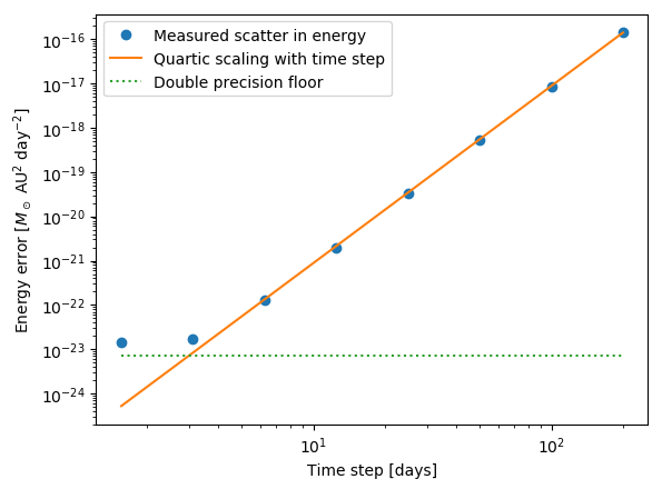
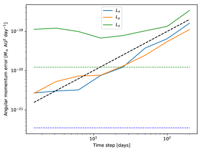
Figure 3: (Top) Conservation of energy. Standard deviation of energy versus step size (blue dots). Orange line shows $h^{4}$ scaling. Green dotted line shows double-precision limit. (Bottom) Angular momentum conservation. The standard deviation of each component is plotted versus step size. The dotted lines shows the double-precision limit for angular momentum ($L_{y}$ is zero, so this is not shown). The black dashed curve shows that angular momentum error scales $\propto h$ according to Brouwer’s law.

5.3 Comparing with C implementation

To check that we have optimized the computational speed of the $N$-body integrator, we carried out a comparison of the Julia version of our code with a C implementation without derivatives (Hernandez, 2016). First, we compared the Kepler solver (Wisdom & Hernandez, 2015) and found that our Julia implementation matches the C version. Both versions take 0.15 $\mu$ sec per Kepler step for a bound orbit with $e=0.5$. Note that in this comparison we used a version of the Kepler step which is not combined with a backward drift.

Next, we carried out an integration of the outer solar system (with 5 bodies, as described in the prior section) with the C implementation. We found that the C implementation runs at the same speed as our Julia implementation of AHL21. With 50-day time steps, both versions take about 4.7 $\mu$sec per timestep. In this comparison, we use the same convergence criterion for the Kepler solver; when we include the 4th-order corrector in AHL21 it increases the run time by $\approx$ 10% for the outer solar system problem. Thus, we conclude that the speed of the Julia implementation is comparable to compiled C.

When using the convergence that a fractional tolerance of $10^{-8}$ is reached for the solution to Kepler’s equation -- we find a bias in the long-term energy conservation which causes it to drift with time. If instead we use the convergence criterion that the eccentric-anomaly, $\gamma$, remains unchanged relative to one of the prior two iterations of Newton’s solver -- then we find that this bias is significantly reduced. This adds iterations to the Kepler-solver, typically 1-2, and thus causes the code to take about 10% longer to run, but with the trade-off of better energy conservation. Thus, using the 4th-order corrector and this criterion adds about 20% to the overall run-time, amounting to 5.7 $\mu$sec per time-step compared with the example above.

Now that we have verified the speed and accuracy of the $N$-body algorithm, we next examine the accuracy and precision of the transit times as a function of step size.

5.4 Transit-timing accuracy

Since the numerical accuracy of the integration depends upon the step size parameter, $h$, as the AHL21 integrator is fourth order in $h$ (Fig. 3), we also expect that the accuracy of transit times should scale with $h^{4}$. Further precision could be obtained if we were to use a corrector at the start of the integration; however, such a corrector is left for future work.

Figure 4 shows the change in the transit times with stepsize for a simulation of TRAPPIST-1 b and c over 400 days. Compared with the times computed with a very small step-size, the transit times drift with time. This behavior is expected due to the difference between the symplectic Hamiltonian and the full Hamiltonian which contains high-frequency terms which cause the coordinates of the symplectic integrator to be offset from the real coordinates. This offset causes the longitudes to drift with time, and due to the slight difference in orbital frequency, the drift grows linearly as shown in Figure 4. Since the AHL21 algorithm has order $h^{4}$, these offsets decrease with step-size as $h^{4}$ (Fig. 4), and so at small stepsize the symplectic integrator better approximates the real system. In practice these coordinate offsets are not expected to be important for transit-timing analyses as they will lead to very small differences between the inferred parameters and real parameters, even for large $h$. We recommend that the user determine which step size is appropriate by checking the difference in transit times as a function of step size.

For the purposes of transit-timing variations, we are primarily interested in the precision of the non-linear portion of the transit times versus epoch. So, to assess the TTV precision, we subtract a linear fit from the difference between an integration with large $h$ with an integration with small $h$, and then compute the RMS of the residuals. We expect the RMS to scale as $h^{4}$, and figure 4 indeed shows that this is the case for large step size for a system with two planets of periods 1.5 and 2.4 days, masses $3\times 10^{-5}$ of the star, low eccentricity, and integrated over 400 days (this approximates the inner two planets of the TRAPPIST-1 system). In both cases the TTV precision reaches a value that is $\approx 10^{-14}$ of each planet’s orbital period. We also find that this precision scales in proportion to the ratio of the masses of the planets to the star, as expected (see discussion under eq. (4)).

Having demonstrated that the accuracy of the transit times scales as expected, we next examine the numerical precision of the computed times, as well as their derivatives.

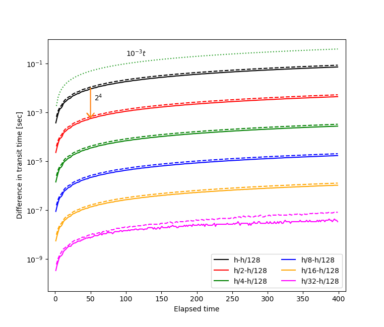
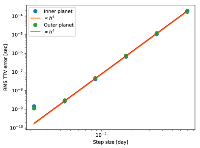
Figure 4: (Left) Variation in the transit times with step size. The absolute value of the difference in times between the indicated step size and a step size of $h/128$ is plotted for the inner two planets of TRAPPIST-1 (solid and dashed, respectively) simulated over 400 days with a nominal step size of $h=0.06$ days. The dotted curve shows a linear scaling, while the arrow indicates a $1/2^{4}$ decrease in timing difference when the step-size is halved. (Right) RMS precision of TTVs for the TRAPPIST-1 b/c two-planet system with six stepsizes, compared with an integration which is $1/2$ of the shortest stepsize, after removing a linear fit from the difference to isolate the comparison to the transit-timing variations. For both planets the TTV errors scale as $h^{4}$ until double-precision is reached at $\approx 10^{-9}$ seconds.

5.5 Precision of transit times and their derivatives

Given a fixed step size for the algorithm, we next ask the question: how numerically precise are the transit times computed for that step size? And, how precise are the derivatives computed as a function of the initial conditions? These questions involve the control of truncation and round-off errors in the algorithm, which motivated the development of the AHL21 algorithm.

We check the numerical precision of the algorithm by comparing the transit times and their derivatives computed at both double-precision and extended precision (using the double-precision Float64 type with 64 bits, and the extended-precision BigFloat type with 256 bits in Julia). Figure 5 shows the difference in the times of transit in the TRAPPIST-1 b and c case computed in double-precision relative to BigFloat precision. We find that the computational errors grow at a rate that is bounded by $\approx 2^{-52}hN_{S}^{3/2}$, where $N_{S}$ is the number of elapsed time steps (Fig. 5), as expected for phase-errors based on Brouwer’s Law (Brouwer, 1937). The computation was carried out for 400,000 days for an inner orbital period of 1.5 days, for a total of $\approx 10^{7}$ time steps.

Next, we carry out tests of the numerical precision of the Jacobians at each substep in the calculation, as well as for the entire integration interval, and for the transit time derivatives. We do this in two ways: 1). by computing finite-difference derivatives in extended precision and 2). by comparing the derivatives in double precision with derivatives computed with extended precision arithmetic. The finite-difference test checks that the formulas derived in §4 are valid, while the extended precision test checks that the numerical implementation is precise.

To compute the finite-difference derivatives, we carry out integrations for each parameter using BigFloat, and compute a finite difference approximation of the partial derivative with parameters perturbed just above and below the nominal value,

$$\frac{\partial t}{\partial q_{i,j}}\approx\frac{\Delta t}{\Delta q_{i,j}}=\frac{t(q_{i,j}(1+\varepsilon_{\mathrm{diff}}))-t(q_{i,j}(1-\varepsilon_{\mathrm{diff}}))}{2\varepsilon_{\mathrm{diff}}q_{i,j}},$$ (89)

where $t(q_{i,j})$ indicates the transit time evaluated at initial conditions $\mathbf{q}_{0}$ with the $i,j$th initial condition given by $q_{i,j}$. Typically we use $\varepsilon_{\mathrm{diff}}=10^{-18}$, and we find that the finite-difference derivative is insensitive to this value when rounded back to double-precision. We used these finite differences in writing and debugging each substep of the code, and we have created a suite of tests which can be used when further modifying or developing the code. We found that the finite difference derivatives agree with the derivatives computed from propagating the Jacobian, at a level close to the double-precision limit, which validates our implementation of the algorithm based on the formulae in §4.

Next, we estimate the fractional numerical errors on the derivatives of the transit times with respect to the initial conditions and masses propagated through the numerical integration (Fig. 5, right panel) by comparing the derivatives computed at double precision with those computed at extended precision. We find that these double-precision numerical errors also shows a growth which is bounded by $2^{-52}N_{S}^{3/2}$, according to Brouwer’s Law. In this case we filtered the derivatives before computing the fractional error taking the maximum absolute value of each derivative over 20 transit times normalized by the maximum absolute derivative over the same 20 times to avoid the case in which the values of the derivatives approach zero. We did not find that the Brouwer’s law limit applied to be the DH17 algorithm - the errors significantly exceeded the Brouwer’s law limit for long integrations - which motivated the development of the AHL21 algorithm. We did not carry out longer integrations due to the high computational expense for BigFloat precision.

We conclude that based on these tests the code is performing as expected: the $N$-body code is fast and as accurate as the algorithm allows; the transit times are precise; the derivative formulae are correct; and the derivatives are precise. With these validations of the code completed, we now turn to compare our code with other publicly-available $N$-body and transit-timing codes.

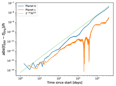
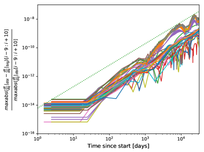
Figure 5: (Left) Fractional numerical error of transit times computed over 40,000 days for TRAPPIST-1 b and c computed from double and BigFloat integrations. The error is plotted relative to the time ste, $h$. (Right) Fractional numerical error on the transit time derivatives with respect to the initial cartesian coordinates and masses. The dotted green lines in both panels scale as $2^{-52}N_{S}^{3/2}$, where $N_{S}$ is the number of time steps. The maximum absolute derivative differences have been taken over 20 steps, and divided by the maximum absolute derivatives to give the fractional differences.

6 Comparison with other codes

In this section we compare with two existing open-source $N$-body integrators which have been used for transit-timing and $N$-body integration: TTVFast and REBOUND. Although other codes are available, such as SYSTEMIC (Meschiari & Laughlin, 2010) and TRADES (Borsato et al., 2014), as well as numerous proprietary codes for modelling transit timing, TTVFast and REBOUND are both widely-used and open-source. These comparisons provide further validation of the accuracy of our code, as well as timing benchmarks of the relative speeds.

6.1 Comparison of transit times with TTVFast and REBOUND

The TTVFast approach uses a Wisdom-Holman integrator (Wisdom & Holman, 1991) with a central dominant body, appropriate for planetary systems orbiting a single star (or planets orbiting a single star in a wide binary). A third-order corrector is used at the start of each simulation to transform from real coordinates to symplectic coordiates. Two versions of TTVFast have been developed in FORTRAN and C; here we describe comparisons with the latter. The initial conditions may be specified in either Jacobi or heliocentric orbital elements, or heliocentric Cartesian coordinates. We use the initial Cartesian coordinates from NbodyGradient transformed to heliocentric coordinates, and then rotated by 180^∘ about the $y$ axis so that the observer is located along the +$z$ axis, the convention adopted in TTVFast.

The TTVFast algorithm uses an approximate method to find times of transit. When a transit time is found to occur for one of the planets between two timesteps, then two Keplerian integrations between the planet and star are integrated forwards and backwards from the prior and subsequent timesteps, and weighted to approximate the position of the planet relative to the star. Newton’s method is then used to find the time of transit in the same manner described above (§4.11).

We have made a comparison of the transit times from NbodyGradient with TTVFast using the best-fit initial conditions for the 7-planet TRAPPIST-1 system (Agol et al., 2021). For this comparison we use a time step for TTVFast which is 0.05% of the orbital period of planet b (Figure 6) to reduce the difference between the symplectic and real coordinates (we use a larger step of 0.1% for NbodyGradient as this integrator is higher precision). We find that over a timescale of $\sim$4532 days (an estimate of the total time between initial and final TRAPPIST-1 observations over the lifetime of JWST), the difference between TTVFast and NbodyGradient is better than a few milliseconds for all seven planets, with better agreement for the inner planets than for the outer. This agreement is quite good, and we attribute the remaining differences, which grow with time, as being due to differences between the initial mapping and real coordinates which cause phase errors to grow with time.

Although REBOUND is not primarily designed for transit-timing, there is a Python notebook in the REBOUND repository which gives an example of transit-time computation. We used the same initial cartesian coordinates as the NbodyGradient computation for TRAPPIST-1, and computed the transit times with a tolerance of $10^{-12}$ days for REBOUND. We transform z$\rightarrow$-x, x$\rightarrow$y, and y$\rightarrow$-z to allow for the fact that the REBOUND computation places the observer along the x axis rather than along the -z axis (as assumed in NbodyGradient, Fig. 2). Figure 6 shows that over 4000 days for TRAPPIST-1, the times agree between NbodyGradient and REBOUND at the $<4\mu$sec level. This was computed with a time step of 0.0015 days for NbodyGradient, about 1/1000 of the orbital period of the inner planet, TRAPPIST-1b, to reduce the difference between the symplectic and real coordinates.

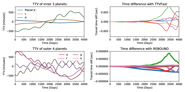
Figure 6: Transit-timing comparison for TRAPPIST-1. (Left) TTVs from NbodyGradient (in color), and TTVFast and REBOUND (black dots) for the seven TRAPPIST-1 planets over 4000 days. (Right) Timing differences in seconds between NbodyGradient and TTVFast (top) and REBOUND (bottom); the colors are same as in left hand panel. Note that the panel in the upper right has a range which has been expanded by $6\times 10^{6}$ relative to the left panels, while the lower right panel is expanded by a factor of $1.2\times 10^{10}$.

Unfortunately TTVFast does not include derivatives, which was part of the motivation for developing the NbodyGradient code. However, given that the transit times compare well, and that we have compared the NbodyGradient derivatives with finite-differences computed at high precision (§5.5), this gives us confidence that the NbodyGradient derivatives are also being computed accurately. We have made scripts available for reproducing this comparison in the NbodyGradient repository.

Next we compare the run-time of NbodyGradient with REBOUND, with and without gradients.

6.2 Run-time Comparison with REBOUND

The REBOUND integrator ias15 (Rein & Tamayo, 2015) allows for the computation of the variational equations, and may be used to model systems with close encounters and an arbitrary architecture. Figure 7 compares the REBOUND ias15 integrator computational speed with our code. We spaced planets by a ratio of semi-major axis of 1.8, and with initial orbital angles separated by 1.4 radians. For the AHL21 integration, we use a step size that is 1/20 of the orbital period of the inner planet and we integrate for 800 orbits of the inner planet. We ran both codes with a range of planets from one to ten, and we turned off the transit finding to make a fair comparison. We tried two different versions of the AHL21 integrator: with fast kicks for pairs of planets, and with fast kicks turned off. When the fast kicks are used for planet pairs, we find that the AHL21 code compares well to REBOUND ias15 algorithm when no gradients are computed, either slightly faster or comparable in wall clock time for 1-10 planets (red and blue dashed lines in Figure 7). However, when the gradient is computed, our code takes a computational time that is $\approx 4-5$ times faster than REBOUND ias15 for a large number of planets when fast kicks are turned off. If the fast-kicks are used for planet pairs, then NbodyGradient is an order of magnitude faster than the ias15 integrator in REBOUND. Note that both REBOUND gradients and NbodyGradient assume the Newtonian equations of motion when computing gradients.

We also compare with the WHFast algorithm in REBOUND. This algorithm is also symplectic, but requires a central dominant mass. The WHFast algorithm is by far the speediest of the three: both with and without gradients it is about an order of magnitude faster than either AHL21 or ias15. However, as it is a second-order algorithm, it may require the use of a corrector, and/or shorter step-sizes, to obtain similar precision as the AHL21 algorithm with is fourth-order; this may come with extra computational cost, depending on the particular application. From a theoretical standpoint, if the Kepler solver function calls dominate the compute time, WHFast should only be twice as fast as AHL21 with kicks between planets in NbodyGradient (green dashed curve). Since we have not achieved this, it may indicate we have not yet properly optimized our code. Julia, NbodyGradient’s language, is believed to be able to achieve speeds comparable to C++, WHFast’s language. We plan to continue to optimize NbodyGradient.

Our primary goal in developing this $N$-body code is for modeling observational data for which the uncertainties are typically dominated by measurement errors rather than model accuracy. Hence, we are willing to exchange some accuracy for computational speed by using a symplectic integrator with a large time step. Thus, AHL21 may provide a useful compromise between ias15 and WHFast. Note that the integrator is still precise, but the symplectic Hamiltonian only approximates the real Hamiltonian, and we have not been able to derive a corrector to transform between symplectic and real coordinates; see the discussion in Deck et al. (2014) and references therein.

In sum, the AHL21 algorithm in NbodyGradient may gain some computation time for general N-body problems with the tradeoff of interpreting the initial conditions as symplectic coordinates, not real coordinates. In addition, currently REBOUND (either ias15 or WHFast) does not yet implement the gradients of the transit times with respect to the initial conditions, which NbodyGradient was designed to compute from the start.

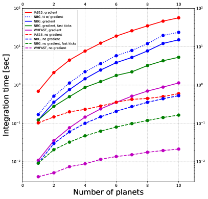
Figure 7: Computational time of the NbodyGradient code without (blue), with fast kicks for planet pairs (green), and with transit-time computation (magenta) versus REBOUND ias15 (red), with (solid) and without (dashed) computation of the gradient. We also compare with the REBOUND WHFast algorithm (magenta), both with gradients (solid) and without (dashed).

7 Summary and conclusions

The original goal of our development of this paper and code was to make possible the analytic computation of the derivatives of the times of transit with respect to the initial conditions; this is the first time this has been done in an $N$-body code to our knowledge. We have accomplished this with a fast and robust code written in the Julia language. Julia has the advantage of matching compiled C speeds if it is written in an optimum manner, which our benchmarks indicate we have achieved. Yet it allows for interactive usage and high-level coding which makes building and debugging the code more straightforward. In addition, Julia easily allows changing of the variable types, so that higher-precision computations are available simply by calling the $N$-body functions with coordinates and masses initialized with high-precision variables; the functions will be automatically recompiled at the first time being called with different numeric types.

We have also developed this code with generality in mind; in particular, we would like to eventually apply it to hierarchical systems such as circumbinary planets or planets hosting moons, which is why we have based the symplectic splitting on the DH17 algorithm which does not assume a dominant body (or bodies). In addition, the popular Wisdom--Holman (WH) method assumes the perturbed approximation holds, which implies the method breaks down during close encounters. The explanation, using error analysis, is that WH has two-body error terms. However, when DH17 is used without kicks, it only has three-body terms which blow up during strong three-body encounters (Dehnen & Hernandez, 2017). So our code can better handle close two-body encounters, as was shown by Dehnen & Hernandez (2017), who used it to simulate a stellar cluster.

However, a drawback of the DH17 algorithm we found was the lack of precision caused by cancellations between the backward drifts and forward Kepler steps. We have fixed this problem by carrying out analytic cancellation of these expressions with modified versions of Gauss’s $f$ and $g$ functions. This fix creates an algorithm which is both numerically stable and precise: energy and angular momentum are conserved well for long integrations. The algorithm is accurate to fourth order in time step, but even for large time steps it will integrate the non-Keplerian perturbations between the bodies with sufficient accuracy for observational data (and the time step can be decreased until the desired precision is reached; this happens rapidly thanks to the fourth-order scaling of the algorithm with time step). This accuracy is higher order than the Wisdom-Holman symplectic integrator or its versions with symplectic correctors, which have error terms scaling as $h^{2}$. As with any symplectic integrator, the integration coordinates are offset slightly from the real coordinates (Wisdom et al., 1996), which causes a long-term phase shift. However, this shift is small, even for large time steps, and should not affect the interpretation of the state of multi-body dynamical systems. In practice it results in a slight offset of the initial coordinates which is caused by introducing high-frequency terms in the physical Hamiltonian.

In order to compute the derivatives of the transit times with respect to the initial conditions, we have propagated the Jacobian of the $N$-body positions and velocities with respect to the initial conditions and masses throughout each timestep of the $N$-body integration. We have eliminated numerical cancellations in this expansion, and used series expansions for special functions when cancellation of the leading orders occurs. This has given an algorithm which yields precise derivatives and which appears to adhere to Brouwer’s law for up to $10^{7}$ timesteps for the problem we tested. We also find that it compares favorably in run time to the variational equations integrated by ias15 (Rein & Tamayo, 2016), with a factor of 4-10 speed-up for long time steps in the comparison we tested.

We have found that the derivatives make possible the optimization of the masses of planets in the TRAPPIST-1 planetary system, and the results compare well with an analysis with the GENGA code (Grimm & Stadel, 2014), as reported in Agol et al. (2021). In particular, we were able to use the derivatives to efficiently find the maximum likelihood and to compute the Hessian at the maximum likelihood. We have also used it to find the likelihood profile as a function of the masses of the planets and orbital parameters, as well as to run a Hamiltonian Markov Chain Monte Carlo computation in 35 dimensions to derive the posterior distribution for the system parameters, which agree well with a complementary analysis based on the code described in Grimm et al. (2018). Finally, the derivatives enabled an efficient search for an eighth planet, which required optimization over 40 free parameters; no strong evidence for an eighth planet turned up in this search (Agol et al., 2021).

These analyses depend on initial conditions which were specified in terms of orbital elements, which we plan to describe in subsequent work. We are also continuing to develop the output options, API, and documentation, and we welcome community contributions to the code repository.

There are some limitations to our work. Due to its symplectic nature, our code does not allow for non-conservative effects to be included, such as tidal forces, drag, or general relativity. However, these could be added in future work through the machinery described by Tamayo et al. (2020). We assume that the masses of the bodies are constant. We do not compute second- or third- order derivatives, as has been implemented by Rein & Tamayo (2016). Even so, we expect this code to find application in a wide range of dynamical problems related to observation of exoplanetary systems and beyond.

Data Availability

No new data were generated or analysed in support of this research. Simulated data which was used for making the figures will be made available in a github repository.

Appendix A Derivation of AHL21 Kepler + Drift step

Here we give more detail for the derivation of the combined Kepler and Drift steps which were described in §3.3. As a reminder, we start with two bodies $i$ and $j$ with relative coordinates $\mathbf{x}_{ij}=\mathbf{x}_{i}-\mathbf{x}_{j}$ and $\mathbf{v}_{ij}=\mathbf{v}_{i}-\mathbf{v}_{j}$. In this section we drop the subscript $ij$. At the start of the time step, the coordinates are $\mathbf{x}_{0}$ and $\mathbf{v}_{0}$, while at the end of the time step the coordinates are $\mathbf{x}$ and $\mathbf{v}$. We propagate these forward with either a negative drift followed by a Kepler step, yielding a change in position and velocity of $\Delta\mathbf{x}_{\mathrm{DK}}$ and $\Delta\mathbf{v}_{\mathrm{DK}}$, or a Kepler step followed by a negative drift, yielding $\Delta\mathbf{x}_{\mathrm{KD}}$ and $\Delta\mathbf{v}_{\mathrm{KD}}$. In the process we need to solve Kepler’s equation 17. The two pathways are shown in Figure 1.

A.1 Drift then Kepler

As discussed in §3, the negative drift is taken first, yielding an intermediate position $\hat{\mathbf{x}}_{0}=\mathbf{x}_{0}-h\mathbf{v}_{0}.$ The resulting change in position and velocity over the time step is given by equation 19,

$$\href https://github.com/ericagol/NbodyGradient.jl/blob/0afa7a5fd387b307e3704ded05ec01838b01478c/src/integrator/ahl21/ahl21.jl#L1022-L1025= \hat{\mathbf{x}}-\mathbf{x}_{0} =(\hat{f}-1)\mathbf{x}_{0}+(\hat{g}-h\hat{f})\mathbf{v}_{0},$$ (90)

$$\href https://github.com/ericagol/NbodyGradient.jl/blob/0afa7a5fd387b307e3704ded05ec01838b01478c/src/integrator/ahl21/ahl21.jl#L1026-L1028= \hat{\mathbf{v}}-\mathbf{v}_{0} =\dot{\hat{f}}\mathbf{x}_{0}+(\dot{\hat{g}}-h\dot{\hat{f}}-1)\mathbf{v}_{0},$$ (91)

where, again, $\hat{f}$, $\hat{g}$, $\dot{\hat{f}}$, and $\dot{\hat{g}}$ are all computed in terms of $(\hat{\mathbf{x}}_{0},\mathbf{v}_{0},k,h)$. This means that the scalar functions these depend on also need to be computed in terms of $\hat{\mathbf{x}}_{0}$, i.e., $\hat{r}_{0}=|\hat{\mathbf{x}}_{0}|,$ $\hat{\beta}=2k/\hat{r}_{0}-v_{0}^{2},$ $\hat{\eta}_{0}=\hat{\mathbf{x}}_{0}\cdot\mathbf{v}_{0},$ and $\hat{G}_{i}=G_{i}(\hat{\beta},\hat{\gamma}),$ where $\hat{\gamma}$ can be computed with Newton’s method from equation (17) evaluated using $\hat{r}_{0}$, $\hat{\eta}_{0}$, and $\hat{G}_{i}$, and $\hat{r}$ can be computed from (16) in the same manner.

The Gauss function terms in equation (19) are given as

$$\href https://github.com/ericagol/NbodyGradient.jl/blob/0afa7a5fd387b307e3704ded05ec01838b01478c/src/integrator/ahl21/ahl21.jl#L994 = -\frac{k}{\hat{r}_{0}}\hat{G}_{2},$$ (92)

$$\href https://github.com/ericagol/NbodyGradient.jl/blob/0afa7a5fd387b307e3704ded05ec01838b01478c/src/integrator/ahl21/ahl21.jl#L998 = k\left(\frac{h}{\hat{r}_{0}}\hat{G}_{2}-\hat{G}_{3}\right),$$ (93)

$$\href https://github.com/ericagol/NbodyGradient.jl/blob/0afa7a5fd387b307e3704ded05ec01838b01478c/src/integrator/ahl21/ahl21.jl#L991 = -\frac{k}{\hat{r}\hat{r}_{0}}\hat{G}_{1},$$ (94)

$$\href https://github.com/ericagol/NbodyGradient.jl/blob/0afa7a5fd387b307e3704ded05ec01838b01478c/src/integrator/ahl21/ahl21.jl#L1014 = \frac{k}{\hat{r}}\left(\frac{h}{\hat{r}_{0}}\hat{G}_{1}-\hat{G}_{2}\right),$$ (95)

where the 1’s have been cancelled analytically for more accurate expressions at small time steps.

A.2 Kepler then Drift

In the case of a Kepler step followed by a negative drift, the Kepler step is computed in terms of the initial coordinates, $\mathbf{x}_{0}$ and $\mathbf{v}_{0}$, yielding intermediate coordinates $(\check{\mathbf{x}},\check{\mathbf{v}})$, and then the negative drift is applied resulting in $\mathbf{x}=\check{\mathbf{x}}-h\check{\mathbf{v}}$ (Figure 1). This yields the change in position and velocity of:

$$\href https://github.com/ericagol/NbodyGradient.jl/blob/0afa7a5fd387b307e3704ded05ec01838b01478c/src/integrator/ahl21/ahl21.jl#L1022-L1025= \check{\mathbf{x}}-h\check{\mathbf{v}}-\mathbf{x}_{0} =(f-h\dot{f}-1)\mathbf{x}_{0}+(g-h\dot{g})\mathbf{v}_{0},$$ (96)

$$\href https://github.com/ericagol/NbodyGradient.jl/blob/0afa7a5fd387b307e3704ded05ec01838b01478c/src/integrator/ahl21/ahl21.jl#L1026-L1028= \check{\mathbf{v}}-\mathbf{v}_{0} =\dot{f}\mathbf{x}_{0}+(\dot{g}-1)\mathbf{v}_{0},$$ (97)

where $f$, $g$, $\dot{f}$, and $\dot{g}$ are all computed in terms of $(\mathbf{x}_{0},\mathbf{v}_{0},k,h)$, and the ‘‘KD" indicates that the Kepler step precedes the negative drift, Kepler-Drift.

These functions can also be expressed in terms of the Gauss functions as

$${f-h\dot{f}-1} = \frac{k}{r}\left(G_{2}-\frac{k}{r_{0}}\left(G_{2}^{2}-G_{1}G_{3}\right)\right),$$ (98)

$$g-h\dot{g} = \frac{k}{r}\left(r_{0}\left(G_{1}G_{2}-G_{0}G_{3}\right)+\eta_{0}\left(G_{2}^{2}-G_{1}G_{3}\right)\right),$$ (99)

$$\href https://github.com/ericagol/NbodyGradient.jl/blob/0afa7a5fd387b307e3704ded05ec01838b01478c/src/integrator/ahl21/ahl21.jl#L991 = -\frac{k}{rr_{0}}G_{1},$$ (100)

$$\href https://github.com/ericagol/NbodyGradient.jl/blob/0afa7a5fd387b307e3704ded05ec01838b01478c/src/integrator/ahl21/ahl21.jl#L1017 = -\frac{k}{r}G_{2},$$ (101)

where we have used equations (17) and (16) to transform these equations. Note that in this case each of these functions depends on $(\mathbf{x}_{0},\mathbf{v}_{0},k,h)$ as the Kepler step is applied before the drift.

Unfortunately these equations can lead to numerical instability for small values of $\gamma=\sqrt{|\beta|}s$. The offending terms involve difference of products of $G_{i}$ functions: $G_{1}G_{2}-G_{0}G_{3}$ and $G_{2}^{2}-G_{1}G_{3}$. These terms have a Taylor series expansion in which the leading order terms in $s$ cancel; this is also true for the function $G_{3}$.

So, we define two new functions,

$$H_{1} = G_{2}^{2}-G_{1}G_{3},$$ (102)

$$H_{2} = G_{1}G_{2}-G_{0}G_{3},$$ (103)

given in Table 1. In terms of these functions we have

$$\href https://github.com/ericagol/NbodyGradient.jl/blob/0afa7a5fd387b307e3704ded05ec01838b01478c/src/integrator/ahl21/ahl21.jl#L1004 = \frac{k}{r}\left(G_{2}-\frac{k}{r_{0}}H_{1}\right),$$ (104)

$$\href https://github.com/ericagol/NbodyGradient.jl/blob/0afa7a5fd387b307e3704ded05ec01838b01478c/src/integrator/ahl21/ahl21.jl#L1007 = \frac{k}{r}\left(r_{0}H_{2}+\eta_{0}H_{1}\right).$$ (105)

For large values of $\gamma$ we evaluate these with the special function definitions, summarized in Table 1, while for small values of $\gamma$, we evaluate $G_{3},H_{1}$ and $H_{2}$ in terms of the following Taylor series:

$$\href https://github.com/ericagol/NbodyGradient.jl/blob/0afa7a5fd387b307e3704ded05ec01838b01478c/src/utils.jl#L180-L209 = \frac{2\gamma^{4}}{\beta^{2}}\sum_{n=0}^{\infty}\frac{(\varepsilon\gamma^{2})^{n}(n+1)}{(2n+4)!},$$ (106)

$$\href https://github.com/ericagol/NbodyGradient.jl/blob/0afa7a5fd387b307e3704ded05ec01838b01478c/src/utils.jl#L225-L254 = \frac{2\gamma^{3}}{|\beta|^{3/2}}\sum_{n=0}^{\infty}\frac{(\varepsilon\gamma^{2})^{n}(n+1)}{(2n+3)!},$$ (107)

$$\href https://github.com/ericagol/NbodyGradient.jl/blob/0afa7a5fd387b307e3704ded05ec01838b01478c/src/utils.jl#L137-L165 = \frac{\gamma^{3}}{|\beta|^{3/2}}\sum_{n=0}^{\infty}\frac{(\varepsilon\gamma^{2})^{n}}{(2n+3)!}.$$ (108)

where $\varepsilon=-1$ for $\beta>0$ (elliptic) and $\varepsilon=1$ for $\beta<0$ (hyperbolic) cases. Note that in evaluating these series expansions we compute each term recursively, and terminate the series expansion when the function matches one of the two prior partial sums (indicating that the series is converged to machine precision).

The fact that these functions have leading terms $\propto\gamma^{3}$ and $\propto\gamma^{4}$ is due to cancellation of lower order terms in the trigonometric representation. This cancellation can lead to round-off errors for small values of $\gamma$, which are commonly encountered when there are a wide range of orbital timescales in a system. We find that higher precision is obtained by evaluating the series expressions for $\gamma<1/2$ out to $\approx 6$ terms in double-precision, while for $\gamma>1/2$, higher precision is obtained from the full trigonometric expression.

The other $G_{i}$ functions ($G_{0},G_{1}$ and $G_{2}$) we evaluate with the stable trigonometric and hyperbolic function transforms discussed in Wisdom & Hernandez (2015), also given in Table 1. With the combination of the drift and Kepler steps, it turns out that we no longer need the drift of the center-of-mass coordinates in each Kepler step as these cancel exactly.

Appendix B Derivation of derivatives of Kepler+Drift steps

In this appendix we give more detail on the derivation of the derivatives of the combined Kepler and drift steps, as well as formulae for the derivatives of the scalar quantities in equations 25, 27, 29, and 31.

B.1 Differential of intermediate quantities

The differentials of $r_{0},\beta,\eta_{0}$ are given by

$$\delta r_{0} = \frac{\mathbf{x}_{0}\cdot\delta\mathbf{x}_{0}}{r_{0}},$$ (109)

$$\delta\beta = \frac{\delta k}{r_{0}}-\frac{k\delta\mathbf{x}_{0}\cdot\mathbf{x}_{0}}{r_{0}^{3}}-2\mathbf{v}_{0}\cdot\delta\mathbf{v}_{0},$$ (110)

$$\delta\eta_{0} = \mathbf{v}_{0}\cdot\delta\mathbf{x}_{0}+\mathbf{x}_{0}\cdot\delta\mathbf{v}_{0}.$$ (111)

Note that these quantities are constant over a time step, and so there is no dependence upon $\delta h$.

Taking the differential of the Universal Kepler equation, 17, we find

$$|\beta|^{-1/2}r\delta\gamma = \delta h+\delta k\left[\frac{D}{r_{0}}-G_{3}\right]$$ (112)

$$- \delta\mathbf{x}_{0}\cdot\left[\left(kD+G_{1}r_{0}^{2}\right)\frac{\mathbf{x}_{0}}{r_{0}^{3}}+G_{2}\mathbf{v}_{0}\right]$$ (113)

$$- \delta\mathbf{v}_{0}\cdot\left[D\mathbf{v}_{0}+G_{2}\mathbf{x}_{0}\right],$$ (114)

$$\href https://github.com/ericagol/NbodyGradient.jl/blob/0afa7a5fd387b307e3704ded05ec01838b01478c/src/integrator/ahl21/ahl21.jl#L1062 = \beta^{-1}\left[h+\eta_{0}G_{2}+2kG_{3}\right].$$ (115)

Note that the $\delta\mathbf{v}_{0}\cdot\mathbf{x}_{0}$ and $\delta\mathbf{x}_{0}\cdot\mathbf{v}_{0}$ have the same derivative terms; this is due to both of these terms deriving from $\delta\eta_{0}$.

Taking the differential of the radial equation, (16), we find

$$\delta r = \frac{\delta\gamma}{|\beta|^{1/2}}(\eta_{0}G_{0}+\zeta G_{1})+\frac{\delta k}{\beta r_{0}}\left(r_{0}-r-kG_{2}\right)$$ (116)

$$+ \delta\mathbf{x}_{0}\cdot\left[\left(kr+k^{2}G_{2}-\zeta r_{0}G_{0}\right)\frac{\mathbf{x}_{0}}{\beta r_{0}^{3}}+G_{1}\mathbf{v}_{0}\right]$$ (117)

$$+ \delta\mathbf{v}_{0}\cdot\left[\left(\eta_{0}G_{1}+2kG_{2}\right)\frac{\mathbf{v}_{0}}{\beta}+G_{1}\mathbf{x}_{0}\right],$$ (118)

where we define

$$\href https://github.com/ericagol/NbodyGradient.jl/blob/0afa7a5fd387b307e3704ded05ec01838b01478c/src/integrator/ahl21/ahl21.j#L900=k-r_{0}\beta.$$ (119)

The functions $G_{i}(\beta,\gamma)$ have derivatives in terms of $\beta$ and $\gamma$, which we can combine with the foregoing differentials for these quantities to obtain the derivatives with respect to the basis $(\mathbf{x}_{0},\mathbf{v}_{0},k,h)$. These intermediate derivatives of $G_{i}$ (in both the elliptic and hyperbolic cases) are given by

$$\frac{\partial G_{i+1}}{\partial\gamma} = \frac{G_{i}}{|\beta|^{1/2}}\ \ (i\geq 0),$$ (120)

$$\frac{\partial G_{0}}{\partial\gamma} = -\frac{\beta G_{1}}{|\beta|^{1/2}},$$ (121)

and

$$\frac{\partial G_{n}}{\partial\beta} = -\frac{n}{2\beta}G_{n}.$$ (122)

With these intermediate derivatives in hand, we can compute the full differentials of the Gauss functions in the combined drift and Kepler terms. Since these formulae differ in the two cases, we consider each separately in turn in the following two subsections.

B.2 Differential of drift-then-Kepler step

The differential of the scalar quantities $\delta(\hat{f}-1)$, $\delta(\hat{g}-h\hat{f}),$ $\delta(\dot{\hat{f}})$, and $\delta(\dot{\hat{g}}-h\dot{\hat{f}}-1)$ should also be scalars, and can be expressed in terms similar to the $\delta\gamma$ and $\delta r$ terms given above. Note, however, that as the Kepler step takes place after the negative drift, all of these functions are to be computed in terms of $\hat{\mathbf{x}}_{0}$ substituted for $\mathbf{x}_{0}$, and so we need to add an extra step in the derivation to find the differentials in terms of $\mathbf{x}_{0}$ in lieu of $\hat{\mathbf{x}}_{0}$.

The differential of these functions in terms of intermediate scalar quantities is given by

$$\frac{\delta(\hat{f}-1)}{\hat{f}-1} = \frac{\delta k}{k}-\frac{\delta\hat{r}_{0}}{\hat{r}_{0}}+\frac{\hat{G}_{1}}{\hat{G}_{2}}\frac{\delta\hat{\gamma}}{|\hat{\beta}|^{1/2}}-\frac{\delta\hat{\beta}}{\hat{\beta}},$$ (123)

$$\delta(\hat{g}-h\hat{f}) = \frac{\delta k}{k}(\hat{g}-h\hat{f})+k\Bigg{[}\left(\frac{\delta h}{\hat{r}_{0}}-\frac{h\delta\hat{r}_{0}}{{\hat{r}_{0}}^{2}}\right)\hat{G}_{2}$$ (124)

$$+ \frac{\delta\hat{\gamma}}{|\hat{\beta}|^{\tfrac{1}{2}}}\left(\frac{h}{\hat{r}_{0}}\hat{G}_{1}-\hat{G}_{2}\right)-\frac{\delta\hat{\beta}}{\hat{\beta}}\left(\frac{h}{\hat{r}_{0}}-\tfrac{3}{2}\hat{G}_{3}\right)\Bigg{]},$$ (125)

$$\frac{\delta\dot{\hat{f}}}{\dot{f}} = \frac{\delta k}{k}-\frac{\delta\hat{r}_{0}}{\hat{r}_{0}}-\frac{\delta\hat{r}}{\hat{r}}+\frac{\hat{G}_{0}}{\hat{G}_{1}}\frac{\delta\hat{\gamma}}{|\hat{\beta}|^{1/2}}-\frac{1}{2}\frac{\delta\hat{\beta}}{\hat{\beta}},$$ (126)

$$\delta(\dot{\hat{g}}-h\dot{\hat{f}}-1) = \left[\frac{\delta k}{\hat{r}_{0}\hat{r}}-\frac{k\delta\hat{r}_{0}}{{\hat{r}_{0}}^{2}\hat{r}}-\frac{k\delta\hat{r}}{\hat{r}_{0}{\hat{r}}^{2}}\right]\left(h\hat{G}_{1}-\hat{r}_{0}\hat{G}_{2}\right)$$ (127)

$$+ \frac{k}{\hat{r}_{0}\hat{r}}\left[\delta h\hat{G}_{1}-\delta\hat{r}_{0}\hat{G}_{2}-\frac{1}{2}\frac{\delta\hat{\beta}}{\hat{\beta}}\left(h\hat{G}_{1}-2\hat{r}_{0}\hat{G}_{2}\right)\right.$$ (128)

$$+ \left.\left(h\hat{G}_{0}-r_{0}\hat{G}_{1}\right)\frac{\delta\hat{\gamma}}{{|\hat{\beta}|^{1/2}}}\right].$$ (129)

In this equation we have used the ‘ $\hat{}$ ’ symbol to indicate that each of these quantities is a function of $\hat{\mathbf{x}}_{0}$ rather than $\mathbf{x}_{0}$ (with the exception of $h$ and $k$). Into these differentials we can substitute our expressions for $\delta\hat{\beta}$, $\delta\hat{r}$, $\delta\hat{r}_{0}$, $\delta\hat{\eta}_{0}$, and $\delta\hat{\gamma}$ given above, keeping in mind that these need to be computed in terms of $\delta\hat{\mathbf{x}}_{0}$ and $\hat{\mathbf{x}}_{0}$ substituted for $\delta\mathbf{x}_{0}$ and $\mathbf{x}_{0}$. Then, we need to replace the differential $\delta\hat{\mathbf{x}}_{0}$ by $\delta\mathbf{x}_{0}-h\delta\mathbf{v}_{0}-\mathbf{v}_{0}\delta h$. The $\mathbf{v}_{0}\delta h$ term leads to dot products of $\mathbf{v}_{0}\cdot\hat{\mathbf{x}}_{0}=\hat{\eta}_{0}$ and $\mathbf{v}_{0}\cdot\mathbf{v}_{0}=\frac{2k}{\hat{r}_{0}}-\hat{\beta}$. The algebraic computation of these operations was aided by Mathematica (Wolfram Research, 2019), yielding the following results:

$$\href https://github.com/ericagol/NbodyGradient.jl/blob/0afa7a5fd387b307e3704ded05ec01838b01478c/src/integrator/ahl21/ahl21.jl#L1112-L1117 = \delta k\mathcal{A}_{k}+\delta h\mathcal{A}_{h}+\delta\mathbf{x}_{0}\cdot\mathbf{x}_{0}\mathcal{A}_{xx}$$ (130)

$$+ \delta(\mathbf{x}_{0}\cdot\mathbf{v}_{0})\mathcal{A}_{xv}+\delta\mathbf{v}_{0}\cdot\mathbf{v}_{0}\mathcal{A}_{vv},$$ (131)

$$\href https://github.com/ericagol/NbodyGradient.jl/blob/0afa7a5fd387b307e3704ded05ec01838b01478c/src/integrator/ahl21/ahl21.jl#L1081 = \frac{1}{k}-\frac{2}{\beta r_{0}}+\frac{c_{1}G_{1}}{rr_{0}G_{2}},$$ (132)

$$\href https://github.com/ericagol/NbodyGradient.jl/blob/0afa7a5fd387b307e3704ded05ec01838b01478c/src/integrator/ahl21/ahl21.jl#L1080 = \frac{G_{1}}{r}\left(\frac{2k}{r_{0}}-\beta+\frac{1}{G_{2}}\right)-c_{24}\eta_{0},$$ (133)

$$\href https://github.com/ericagol/NbodyGradient.jl/blob/0afa7a5fd387b307e3704ded05ec01838b01478c/src/integrator/ahl21/ahl21.jl#L1075 = c_{24},$$ (134)

$$\href https://github.com/ericagol/NbodyGradient.jl/blob/0afa7a5fd387b307e3704ded05ec01838b01478c/src/integrator/ahl21/ahl21.jl#L1076 = -\left[c_{24}h+\frac{G_{1}}{r}\right],$$ (135)

$$\href https://github.com/ericagol/NbodyGradient.jl/blob/0afa7a5fd387b307e3704ded05ec01838b01478c/src/integrator/ahl21/ahl21.jl#L1079 = \frac{1}{r}\left[\frac{kH_{6}}{\beta G_{2}}-r_{0}G_{2}+h\left(2G_{1}+hrc_{24}\right)\right],$$ (136)

$$\href https://github.com/ericagol/NbodyGradient.jl/blob/0afa7a5fd387b307e3704ded05ec01838b01478c/src/integrator/ahl21/ahl21.jl#L1112-L1117 = \delta k\mathcal{B}_{k}+\delta h\mathcal{B}_{h}+\delta\mathbf{x}_{0}\cdot\mathbf{x}_{0}\mathcal{B}_{xx}$$ (137)

$$+ \delta(\mathbf{x}_{0}\cdot\mathbf{v}_{0})\mathcal{B}_{xv}+\delta\mathbf{v}_{0}\cdot\mathbf{v}_{0}\mathcal{B}_{vv},$$ (138)

$$\href https://github.com/ericagol/NbodyGradient.jl/blob/0afa7a5fd387b307e3704ded05ec01838b01478c/src/integrator/ahl21/ahl21.jl#L1103 = -\frac{c_{9}k}{\beta r_{0}^{2}}+\frac{c_{1}c_{13}k}{rr_{0}^{2}}+\frac{G_{2}h-G_{3}r_{0}}{r_{0}},$$ (139)

$$\href https://github.com/ericagol/NbodyGradient.jl/blob/0afa7a5fd387b307e3704ded05ec01838b01478c/src/integrator/ahl21/ahl21.jl#L1102 = \frac{kG_{2}}{r_{0}}+\frac{kc_{13}}{rr_{0}}+\frac{kG_{2}c_{13}}{rr_{0}}\left(\frac{2k}{r_{0}}-\beta\right)-\eta_{0}c_{10},$$ (140)

$$\href https://github.com/ericagol/NbodyGradient.jl/blob/0afa7a5fd387b307e3704ded05ec01838b01478c/src/integrator/ahl21/ahl21.jl#L1093 = c_{10},$$ (141)

$$\href https://github.com/ericagol/NbodyGradient.jl/blob/0afa7a5fd387b307e3704ded05ec01838b01478c/src/integrator/ahl21/ahl21.jl#L1094 = -\left[c_{10}h+\frac{c_{13}G_{2}k}{rr_{0}}\right],$$ (142)

$$\href https://github.com/ericagol/NbodyGradient.jl/blob/0afa7a5fd387b307e3704ded05ec01838b01478c/src/integrator/ahl21/ahl21.jl#L1100-L1101 = \frac{2hkG_{2}c_{13}}{rr_{0}}+h^{2}c_{10}$$ (143)

$$+ \frac{k}{\beta rr_{0}}\left[r_{0}^{2}H_{8}-\beta hr_{0}G_{2}^{2}+(hk+\eta_{0}r_{0})H_{6}\right],$$ (144)

$$\href https://github.com/ericagol/NbodyGradient.jl/blob/0afa7a5fd387b307e3704ded05ec01838b01478c/src/integrator/ahl21/ahl21.jl#L1166-L1171 = \delta k\mathcal{C}_{k}+\delta h\mathcal{C}_{h}+\delta\mathbf{x}_{0}\cdot\mathbf{x}_{0}\mathcal{C}_{xx}$$ (145)

$$+ \delta(\mathbf{x}_{0}\cdot\mathbf{v}_{0})\mathcal{C}_{xv}+\delta\mathbf{v}_{0}\cdot\mathbf{v}_{0}\mathcal{C}_{vv},$$ (146)

$$\href https://github.com/ericagol/NbodyGradient.jl/blob/0afa7a5fd387b307e3704ded05ec01838b01478c/src/integrator/ahl21/ahl21.jl#L1142 = \frac{1}{k}-\frac{1}{\beta r_{0}}-\frac{c_{17}}{\beta rr_{0}}-\frac{c_{1}(G_{1}c_{2}-G_{0}r)}{r^{2}r_{0}G_{1}},$$ (147)

$$\href https://github.com/ericagol/NbodyGradient.jl/blob/0afa7a5fd387b307e3704ded05ec01838b01478c/src/integrator/ahl21/ahl21.jl#L1147 = c_{22}\left(\frac{2k}{r_{0}}-\beta\right)-\frac{c_{2}}{r^{2}}+c_{21}\eta_{0}+\frac{G_{0}}{G_{1}r},$$ (148)

$$\href https://github.com/ericagol/NbodyGradient.jl/blob/0afa7a5fd387b307e3704ded05ec01838b01478c/src/integrator/ahl21/ahl21.jl#L1135 = c_{21},$$ (149)

$$\href https://github.com/ericagol/NbodyGradient.jl/blob/0afa7a5fd387b307e3704ded05ec01838b01478c/src/integrator/ahl21/ahl21.jl#L1136 = c_{22}-c_{21}h,$$ (150)

$$\href https://github.com/ericagol/NbodyGradient.jl/blob/0afa7a5fd387b307e3704ded05ec01838b01478c/src/integrator/ahl21/ahl21.jl#L1141 = c_{34}-2hc_{22}+h^{2}c_{21},$$ (151)

$$\href https://github.com/ericagol/NbodyGradient.jl/blob/0afa7a5fd387b307e3704ded05ec01838b01478c/src/integrator/ahl21/ahl21.jl#L1166-L1171 = \delta k\mathcal{D}_{k}+\delta h\mathcal{D}_{h}+\delta\mathbf{x}_{0}\cdot\mathbf{x}_{0}\mathcal{D}_{xx}$$ (152)

$$+ \delta(\mathbf{x}_{0}\cdot\mathbf{v}_{0})\mathcal{D}_{xv}+\delta\mathbf{v}_{0}\cdot\mathbf{v}_{0}\mathcal{D}_{vv},$$ (153)

$$\href https://github.com/ericagol/NbodyGradient.jl/blob/0afa7a5fd387b307e3704ded05ec01838b01478c/src/integrator/ahl21/ahl21.jl#L1156 = \frac{1}{rr_{0}}\Bigg{[}-\frac{k(c_{13}-G_{2}r_{0})}{\beta r_{0}}+c_{13}$$ (154)

$$- \frac{kc_{13}c_{17}}{\beta rr_{0}}+\frac{kc_{1}c_{12}}{rr_{0}}-\frac{kc_{1}c_{2}c_{13}}{r^{2}r_{0}}\Bigg{]},$$ (155)

$$\href https://github.com/ericagol/NbodyGradient.jl/blob/0afa7a5fd387b307e3704ded05ec01838b01478c/src/integrator/ahl21/ahl21.jl#L1161 = \frac{kG_{1}}{rr_{0}}+\frac{kc_{12}}{r^{2}r_{0}}-\frac{kc_{13}c_{2}}{r^{3}r_{0}}$$ (156)

$$- c_{26}\left(\frac{2k}{r_{0}}-\beta\right)-c_{25}\eta_{0},$$ (157)

$$\href https://github.com/ericagol/NbodyGradient.jl/blob/0afa7a5fd387b307e3704ded05ec01838b01478c/src/integrator/ahl21/ahl21.jl#L1148 = c_{25},$$ (158)

$$\href https://github.com/ericagol/NbodyGradient.jl/blob/0afa7a5fd387b307e3704ded05ec01838b01478c/src/integrator/ahl21/ahl21.jl#L1149 = c_{26}-c_{25}h,$$ (159)

$$\href https://github.com/ericagol/NbodyGradient.jl/blob/0afa7a5fd387b307e3704ded05ec01838b01478c/src/integrator/ahl21/ahl21.jl#L1155 = c_{33}+c_{25}h^{2}-2c_{26}h,$$ (160)

with auxiliary quantities defined as

$$\href https://github.com/ericagol/NbodyGradient.jl/blob/0afa7a5fd387b307e3704ded05ec01838b01478c/src/integrator/ahl21/ahl21.jl#L1063 = D-r_{0}G_{3},$$ (161)

$$\href https://github.com/ericagol/NbodyGradient.jl/blob/0afa7a5fd387b307e3704ded05ec01838b01478c/src/integrator/ahl21/ahl21.jl#L1064 = \eta_{0}G_{0}+G_{1}\zeta,$$ (162)

$$\href https://github.com/ericagol/NbodyGradient.jl/blob/0afa7a5fd387b307e3704ded05ec01838b01478c/src/integrator/ahl21/ahl21.jl#L1065 = Dk+G_{1}r_{0}^{2},$$ (163)

$$\href https://github.com/ericagol/NbodyGradient.jl/blob/0afa7a5fd387b307e3704ded05ec01838b01478c/src/integrator/ahl21/ahl21.jl#L1066 = \eta_{0}G_{1}+2G_{0}r_{0},$$ (164)

$$\href https://github.com/ericagol/NbodyGradient.jl/blob/0afa7a5fd387b307e3704ded05ec01838b01478c/src/integrator/ahl21/ahl21.jl#L1122 = \frac{r_{0}-kG_{2}}{rG_{1}},$$ (165)

$$\href https://github.com/ericagol/NbodyGradient.jl/blob/0afa7a5fd387b307e3704ded05ec01838b01478c/src/integrator/ahl21/ahl21.jl#L1123 = \frac{r_{0}G_{0}-kG_{2}}{\beta},$$ (166)

$$\href https://github.com/ericagol/NbodyGradient.jl/blob/0afa7a5fd387b307e3704ded05ec01838b01478c/src/integrator/ahl21/ahl21.jl#L1124 = G_{2}\left(\frac{1}{G_{1}}+\frac{c_{2}}{r}\right),$$ (167)

$$\href https://github.com/ericagol/NbodyGradient.jl/blob/0afa7a5fd387b307e3704ded05ec01838b01478c/src/integrator/ahl21/ahl21.jl#L1125 = r_{0}^{-3}\left(kc_{6}+rr_{0}+c_{3}c_{5}\right),$$ (168)

$$\href https://github.com/ericagol/NbodyGradient.jl/blob/0afa7a5fd387b307e3704ded05ec01838b01478c/src/integrator/ahl21/ahl21.jl#L1070 = 2hG_{2}-3r_{0}G_{3},$$ (169)

$$\href https://github.com/ericagol/NbodyGradient.jl/blob/0afa7a5fd387b307e3704ded05ec01838b01478c/src/integrator/ahl21/ahl21.jl#L1071 = \frac{k}{r_{0}^{4}}\left[-G_{2}r_{0}h+\frac{kc_{9}}{\beta}-\frac{c_{3}c_{13}}{r}\right],$$ (170)

$$\href https://github.com/ericagol/NbodyGradient.jl/blob/0afa7a5fd387b307e3704ded05ec01838b01478c/src/integrator/ahl21/ahl21.jl#L1126 = G_{0}h-G_{1}r_{0},$$ (171)

$$\href https://github.com/ericagol/NbodyGradient.jl/blob/0afa7a5fd387b307e3704ded05ec01838b01478c/src/integrator/ahl21/ahl21.jl#L1067 = G_{1}h-G_{2}r_{0},$$ (172)

$$\href https://github.com/ericagol/NbodyGradient.jl/blob/0afa7a5fd387b307e3704ded05ec01838b01478c/src/integrator/ahl21/ahl21.jl#L1127 = r_{0}-r-kG_{2},$$ (173)

$$\href https://github.com/ericagol/NbodyGradient.jl/blob/0afa7a5fd387b307e3704ded05ec01838b01478c/src/integrator/ahl21/ahl21.jl#L1128 = \eta_{0}G_{1}+2kG_{2},$$ (174)

$$\href https://github.com/ericagol/NbodyGradient.jl/blob/0afa7a5fd387b307e3704ded05ec01838b01478c/src/integrator/ahl21/ahl21.jl#L1129 = k(kG_{2}+r)-G_{0}r_{0}\zeta,$$ (175)

$$\href https://github.com/ericagol/NbodyGradient.jl/blob/0afa7a5fd387b307e3704ded05ec01838b01478c/src/integrator/ahl21/ahl21.jl#L1130 = \frac{(kG_{2}-r_{0})(\beta c_{3}-kG_{1}r)}{\beta r^{2}r_{0}^{3}G_{1}}+\frac{\eta_{0}G_{1}}{rr_{0}^{2}}-\frac{2}{r_{0}^{2}},$$ (176)

$$\href https://github.com/ericagol/NbodyGradient.jl/blob/0afa7a5fd387b307e3704ded05ec01838b01478c/src/integrator/ahl21/ahl21.jl#L1131 = \frac{1}{r}\left[-G_{1}-\frac{G_{0}G_{2}}{G_{1}}+\frac{G_{2}c_{2}}{r}\right],$$ (177)

$$\href https://github.com/ericagol/NbodyGradient.jl/blob/0afa7a5fd387b307e3704ded05ec01838b01478c/src/integrator/ahl21/ahl21.jl#L1072 = \frac{1}{r_{0}^{3}}\left[r_{0}\left(\frac{2k}{\beta r_{0}}-1\right)-\frac{G_{1}c_{3}}{rG_{2}}\right],$$ (178)

$$\href https://github.com/ericagol/NbodyGradient.jl/blob/0afa7a5fd387b307e3704ded05ec01838b01478c/src/integrator/ahl21/ahl21.jl#L1132-L1133 = \frac{k}{rr_{0}^{2}}\Bigg{[}-G_{2}+\frac{k(c_{13}-G_{2}r_{0})}{\beta r_{0}^{2}}-\frac{c_{13}}{r_{0}}-\frac{c_{12}c_{3}}{rr_{0}^{2}}$$ (179)

$$+ \frac{c_{13}c_{2}c_{3}}{r^{2}r_{0}^{2}}-\frac{c_{13}(k(kG_{2}+r)-G_{0}r_{0}\zeta)}{\beta rr_{0}^{2}}\Bigg{]},$$ (180)

$$\href https://github.com/ericagol/NbodyGradient.jl/blob/0afa7a5fd387b307e3704ded05ec01838b01478c/src/integrator/ahl21/ahl21.jl#L1134 = \frac{k}{r^{2}r_{0}}\left[-G_{2}c_{12}-G_{1}c_{13}+\frac{G_{2}c_{13}c_{2}}{r}\right],$$ (181)

$$\href https://github.com/ericagol/NbodyGradient.jl/blob/0afa7a5fd387b307e3704ded05ec01838b01478c/src/integrator/ahl21/ahl21.jl#L1154 = \frac{Dk^{2}}{r^{3}r_{0}}(hG_{2}-r_{0}G_{3})$$ (182)

$$+ \frac{k}{\beta r^{2}r_{0}}\Big{[}-\eta_{0}kG_{1}G_{2}^{2}-G_{1}G_{2}G_{3}k^{2}$$ (183)

$$- r_{0}\eta_{0}\beta G_{1}G_{2}^{2}-r_{0}kG_{1}H_{2}-\beta G_{2}^{2}G_{0}r_{0}^{2}\Big{]},$$ (184)

$$\href https://github.com/ericagol/NbodyGradient.jl/blob/0afa7a5fd387b307e3704ded05ec01838b01478c/src/integrator/ahl21/ahl21.jl#L1139-L1140 = \frac{1}{\beta r^{2}}\Big{[}-\beta(\eta_{0}G_{2}+r_{0}G_{1})^{2}-\eta_{0}kH_{8}-H_{6}k^{2}$$ (185)

$$+ (G_{2}^{2}-3G_{1}G_{3})\beta kr_{0}\Big{]}+\frac{\eta_{0}G_{2}^{2}}{rG_{1}}+\frac{kH_{8}}{\beta rG_{1}},$$ (186)

where we have dropped the $\hat{}$ superscript on the right hand side of equations 136-186 for legibility, but note that all scalar quantities in these equations which are a function of $\mathbf{x}_{0}$ must be evaluated as a function of $\hat{\mathbf{x}}_{0}$ in lieu of $\mathbf{x}_{0}$. In these equations, we have taken care to analytically cancel terms to leading order in $\gamma$ by defining the following functions

$$\href https://github.com/ericagol/NbodyGradient.jl/blob/0afa7a5fd387b307e3704ded05ec01838b01478c/src/utils.jl#L256-L269 = G_{1}G_{2}-3G_{3},$$ (187)

$$\href https://github.com/ericagol/NbodyGradient.jl/blob/0afa7a5fd387b307e3704ded05ec01838b01478c/src/integrator/ahl21/ahl21.jl#L1083 = -\beta H_{1},$$ (188)

$$\href https://github.com/ericagol/NbodyGradient.jl/blob/0afa7a5fd387b307e3704ded05ec01838b01478c/src/utils.jl#L305-L318 = G_{1}G_{2}-(2+G_{0})G_{3},$$ (189)

$$\href https://github.com/ericagol/NbodyGradient.jl/blob/0afa7a5fd387b307e3704ded05ec01838b01478c/src/utils.jl#L351-L362 = 2G_{2}^{2}-3G_{1}G_{3},$$ (190)

$$\href https://github.com/ericagol/NbodyGradient.jl/blob/0afa7a5fd387b307e3704ded05ec01838b01478c/src/integrator/ahl21/ahl21.jl#L1261 = G_{1}G_{2}-2G_{0}G_{1}G_{2}+3G_{0}^{2}G_{3}=\beta G_{1}G_{2}^{2}-G_{0}H_{8},$$ (191)

$$\href https://github.com/ericagol/NbodyGradient.jl/blob/0afa7a5fd387b307e3704ded05ec01838b01478c/src/integrator/ahl21/ahl21.jl#L1099 = G_{1}G_{2}-3G_{0}G_{3}=-2H_{3}+3H_{5}.$$ (192)

These functions are tabulated in Table 1. As with $G_{3},H_{1}$ and $H_{2}$, for small values of $\gamma$ we evaluate these with a series expansion:

$$\href https://github.com/ericagol/NbodyGradient.jl/blob/0afa7a5fd387b307e3704ded05ec01838b01478c/src/utils.jl#L271-L303 = -\frac{4\gamma^{5}}{\beta|\beta|^{1/2}}\sum_{n=0}^{\infty}\frac{(\varepsilon\gamma^{2})^{n}(4^{n+1}-1)}{(2n+5)!},$$ (193)

$$\href https://github.com/ericagol/NbodyGradient.jl/blob/0afa7a5fd387b307e3704ded05ec01838b01478c/src/utils.jl#L320-L349 = -\frac{2\gamma^{5}}{\beta|\beta|^{1/2}}\sum_{n=0}^{\infty}\frac{(\varepsilon\gamma^{2})^{n}(n+1)}{(2n+5)!},$$ (194)

$$\href https://github.com/ericagol/NbodyGradient.jl/blob/0afa7a5fd387b307e3704ded05ec01838b01478c/src/utils.jl#L364-L396 = \frac{2\gamma^{6}}{\beta^{2}}\sum_{n=0}^{\infty}\frac{(\varepsilon\gamma^{2})^{n}\left(4^{n+2}-3n-7\right)}{(2n+6)!},$$ (195)

where $\varepsilon=-1$ for $\beta>0$ (elliptic) and $\varepsilon=1$ for $\beta<0$ (hyperbolic) cases. The coefficients of these series are computed recursively for efficiency. Note that we found expressions for $H_{4}$, $H_{7}$, and $H_{8}$ in terms of the other $G$ and $H$ functions.

B.3 Differential of Kepler then drift step

The Kepler step followed by a negative drift is slightly simpler as the Gauss functions can be expressed in terms of $\mathbf{x}_{0}$ rather than $\hat{\mathbf{x}}_{0}$. The differential of the scalar functions are given by

$$\href https://github.com/ericagol/NbodyGradient.jl/blob/0afa7a5fd387b307e3704ded05ec01838b01478c/src/integrator/ahl21/ahl21.jl#L1270-L1277 = \delta k\mathcal{E}_{k}+\delta h\mathcal{E}_{h}+\delta\mathbf{x}_{0}\cdot\mathbf{x}_{0}\mathcal{E}_{xx}$$ (196)

$$+ \delta(\mathbf{x}_{0}\cdot\mathbf{v}_{0})\mathcal{E}_{xv}+\delta\mathbf{v}_{0}\cdot\mathbf{v}_{0}\mathcal{E}_{vv},$$ (197)

$$\href https://github.com/ericagol/NbodyGradient.jl/blob/0afa7a5fd387b307e3704ded05ec01838b01478c/src/integrator/ahl21/ahl21.jl#L1242-L1243 = \frac{k}{rr_{0}}\Big{[}-\frac{c_{14}c_{17}}{\beta rr_{0}}-\frac{2G_{2}}{\beta}+\frac{4H_{1}k}{\beta r_{0}}$$ (198)

$$- \frac{c_{1}c_{14}c_{2}}{r^{2}r_{0}}+\frac{c_{1}(G_{1}r_{0}-H_{2}k)}{rr_{0}}+\frac{c_{14}}{k}-H_{1}\Big{]},$$ (199)

$$\href https://github.com/ericagol/NbodyGradient.jl/blob/0afa7a5fd387b307e3704ded05ec01838b01478c/src/integrator/ahl21/ahl21.jl#L1241 = \frac{k}{r^{2}}\left[-\frac{c_{14}c_{2}}{rr_{0}}+G_{1}-\frac{H_{2}k}{r_{0}}\right],$$ (200)

$$\href https://github.com/ericagol/NbodyGradient.jl/blob/0afa7a5fd387b307e3704ded05ec01838b01478c/src/integrator/ahl21/ahl21.jl#L1234 = \frac{k}{\beta r^{3}r_{0}^{4}}\Big{[}\beta c_{3}(c_{14}c_{2}+c_{23}r)+H_{1}kr^{2}r_{0}\left(\beta-\frac{2k}{r_{0}}\right)$$ (201)

$$+ c_{14}r\Big{(}G_{0}r_{0}\zeta+k(r-G_{2}k)\Big{)}\Big{]},$$ (202)

$$\href https://github.com/ericagol/NbodyGradient.jl/blob/0afa7a5fd387b307e3704ded05ec01838b01478c/src/integrator/ahl21/ahl21.jl#L1235 = \frac{k}{r^{2}r_{0}}\Big{[}\frac{c_{14}c_{2}G_{2}}{r}+k(G_{1}H_{1}+G_{2}H_{2})-2G_{1}G_{2}r_{0}\Big{]},$$ (203)

$$\href https://github.com/ericagol/NbodyGradient.jl/blob/0afa7a5fd387b307e3704ded05ec01838b01478c/src/integrator/ahl21/ahl21.jl#L1238-L1240 = \frac{k}{\beta r^{2}r_{0}}\Big{[}2\eta_{0}k(G_{2}G_{3}-G_{1}H_{1})$$ (204)

$$+ (3G_{3}H_{2}-4H_{1}G_{2})k^{2}+\beta G_{2}r_{0}(3H_{1}k-G_{2}r_{0})$$ (205)

$$+ \frac{c_{14}}{r}\Big{(}-\beta(G_{2}\eta+G_{1}r_{0})^{2}+\eta_{0}k(2G_{0}G_{3}-H_{2})$$ (206)

$$+ k\beta r_{0}(H_{1}-2G_{1}G_{3})-H_{6}k^{2}\Big{)}\Big{]},$$ (207)

$$\href https://github.com/ericagol/NbodyGradient.jl/blob/0afa7a5fd387b307e3704ded05ec01838b01478c/src/integrator/ahl21/ahl21.jl#L1271-L1277 = \delta k\mathcal{F}_{k}+\delta h\mathcal{F}_{h}+\delta\mathbf{x}_{0}\cdot\mathbf{x}_{0}\mathcal{F}_{xx}$$ (208)

$$+ \delta(\mathbf{x}_{0}\cdot\mathbf{v}_{0})\mathcal{F}_{xv}+\delta\mathbf{v}_{0}\cdot\mathbf{v}_{0}\mathcal{F}_{vv},$$ (209)

$$\href https://github.com/ericagol/NbodyGradient.jl/blob/0afa7a5fd387b307e3704ded05ec01838b01478c/src/integrator/ahl21/ahl21.jl#L1258 = \frac{k}{r}\left[\frac{c_{15}}{k}-\frac{c_{15}c_{17}}{\beta rr_{0}}-\frac{c_{19}}{\beta r_{0}}-\frac{c_{1}c_{15}c_{2}}{r^{2}r_{0}}+\frac{c_{1}c_{16}}{rr_{0}}\right],$$ (210)

$$\href https://github.com/ericagol/NbodyGradient.jl/blob/0afa7a5fd387b307e3704ded05ec01838b01478c/src/integrator/ahl21/ahl21.jl#L1267 = \frac{k}{r^{3}}\left[c_{16}r-c_{15}c_{2}\right],$$ (211)

$$\href https://github.com/ericagol/NbodyGradient.jl/blob/0afa7a5fd387b307e3704ded05ec01838b01478c/src/integrator/ahl21/ahl21.jl#L1250 = \frac{k}{rr_{0}}\Bigg{[}-\frac{c_{15}(k(G_{2}k+r)-G_{0}r_{0}\zeta)}{\beta rr_{0}^{2}}+\frac{c_{19}k}{\beta r_{0}^{2}}$$ (212)

$$+ \frac{c_{15}c_{2}c_{3}}{r^{2}r_{0}^{2}}-\frac{c_{16}c_{3}}{rr_{0}^{2}}+H_{2}\Bigg{]},$$ (213)

$$\href https://github.com/ericagol/NbodyGradient.jl/blob/0afa7a5fd387b307e3704ded05ec01838b01478c/src/integrator/ahl21/ahl21.jl#L1251 = \frac{k}{r^{2}}\left[\frac{c_{15}c_{2}G_{2}}{r}-c_{15}G_{1}-c_{16}G_{2}+H_{1}r\right],$$ (214)

$$\href https://github.com/ericagol/NbodyGradient.jl/blob/0afa7a5fd387b307e3704ded05ec01838b01478c/src/integrator/ahl21/ahl21.jl#L1254-L1257 = \frac{k}{\beta r^{2}}\Big{[}2\eta_{0}^{2}(G_{1}H_{1}-G_{2}G_{3})+\eta_{0}k(4G_{2}H_{1}-3H_{2}G_{3})$$ (215)

$$+ r_{0}\eta_{0}(4G_{0}H_{1}-2G_{1}G_{3})$$ (216)

$$+ 3r_{0}k\big{(}(G_{1}+\beta G_{3})H_{1}-G_{3}G_{2}\big{)}$$ (217)

$$+ \big{(}G_{0}H_{8}-\beta G_{1}(G_{2}^{2}+G_{1}G_{3})\big{)}r_{0}^{2}$$ (218)

$$- \frac{c_{15}}{r}\Big{(}\beta G_{2}^{2}\eta_{0}^{2}+\eta_{0}kH_{8}+H_{6}k^{2}+\beta G_{1}^{2}r_{0}^{2}$$ (219)

$$+ \big{(}2\eta_{0}G_{1}G_{2}-k(G_{2}^{2}-3G_{1}G_{3})\big{)}\beta r_{0}\Big{)}\Big{]},$$ (220)

$$\href https://github.com/ericagol/NbodyGradient.jl/blob/0afa7a5fd387b307e3704ded05ec01838b01478c/src/integrator/ahl21/ahl21.jl#L1312-L1319 = \delta k\mathcal{G}_{k}+\delta h\mathcal{G}_{h}+\delta\mathbf{x}_{0}\cdot\mathbf{x}_{0}\mathcal{G}_{xx}$$ (221)

$$+ \delta(\mathbf{x}_{0}\cdot\mathbf{v}_{0})\mathcal{G}_{xv}+\delta\mathbf{v}_{0}\cdot\mathbf{v}_{0}\mathcal{G}_{vv},$$ (222)

$$\href https://github.com/ericagol/NbodyGradient.jl/blob/0afa7a5fd387b307e3704ded05ec01838b01478c/src/integrator/ahl21/ahl21.jl#L1292 = \frac{1}{k}+\frac{c_{1}(r_{0}-kG_{2})}{r_{0}r^{2}G_{1}}-\frac{r+c_{17}}{\beta rr0},$$ (223)

$$\href https://github.com/ericagol/NbodyGradient.jl/blob/0afa7a5fd387b307e3704ded05ec01838b01478c/src/integrator/ahl21/ahl21.jl#L1297 = \frac{r_{0}-kG_{2}}{r^{2}G_{1}},$$ (224)

$$\href https://github.com/ericagol/NbodyGradient.jl/blob/0afa7a5fd387b307e3704ded05ec01838b01478c/src/integrator/ahl21/ahl21.jl#L1286 = \frac{1}{r_{0}^{2}}\Bigg{[}-\frac{k(G_{2}k-r_{0})}{\beta rr_{0}}+\frac{c_{2}c_{3}}{r^{2}r_{0}}-\frac{c_{3}G_{0}}{G_{1}rr_{0}}$$ (225)

$$+ \frac{\eta_{0}G_{1}}{r}-2\Bigg{]},$$ (226)

$$\href https://github.com/ericagol/NbodyGradient.jl/blob/0afa7a5fd387b307e3704ded05ec01838b01478c/src/integrator/ahl21/ahl21.jl#L1287 = -\frac{1}{r}\left(\frac{G_{0}G_{2}}{G_{1}}+\frac{r_{0}G_{1}+\eta_{0}G_{2}}{r}\right),$$ (227)

$$\href https://github.com/ericagol/NbodyGradient.jl/blob/0afa7a5fd387b307e3704ded05ec01838b01478c/src/integrator/ahl21/ahl21.jl#L1290-L1291 = \frac{1}{\beta r^{2}}\Bigg{[}\frac{(\eta_{0}G_{2}^{2}\beta+kH_{8})(r_{0}G_{0}+kG_{2})}{G_{1}}-H_{6}k^{2}$$ (228)

$$+ \beta r_{0}\left(k(H_{1}-2G_{1}G_{3})-2\eta_{0}G_{1}G_{2}\right)-\beta G_{1}^{2}r_{0}^{2}\Bigg{]},$$ (229)

$$\href https://github.com/ericagol/NbodyGradient.jl/blob/0afa7a5fd387b307e3704ded05ec01838b01478c/src/integrator/ahl21/ahl21.jl#L1314-L1319 = \delta k\mathcal{H}_{k}+\delta h\mathcal{H}_{h}+\delta\mathbf{x}_{0}\cdot\mathbf{x}_{0}\mathcal{H}_{xx}$$ (230)

$$+ \delta(\mathbf{x}_{0}\cdot\mathbf{v}_{0})\mathcal{H}_{xv}+\delta\mathbf{v}_{0}\cdot\mathbf{v}_{0}\mathcal{H}_{vv},$$ (231)

$$\href https://github.com/ericagol/NbodyGradient.jl/blob/0afa7a5fd387b307e3704ded05ec01838b01478c/src/integrator/ahl21/ahl21.jl#L1304 = \frac{1}{rr_{0}}\Bigg{[}\frac{G_{2}k(-G_{2}k+r+r_{0})}{\beta r}+\frac{c_{1}c_{2}G_{2}k}{r^{2}}$$ (232)

$$- \frac{c_{1}G_{1}k}{r}-G_{2}r_{0}\Bigg{]},$$ (233)

$$\href https://github.com/ericagol/NbodyGradient.jl/blob/0afa7a5fd387b307e3704ded05ec01838b01478c/src/integrator/ahl21/ahl21.jl#L1309 = \frac{k}{r^{3}}\left[c_{2}G_{2}-G_{1}r\right],$$ (234)

$$\href https://github.com/ericagol/NbodyGradient.jl/blob/0afa7a5fd387b307e3704ded05ec01838b01478c/src/integrator/ahl21/ahl21.jl#L1298 = \frac{k}{r^{2}r_{0}^{3}}\Bigg{[}\frac{G_{2}(k(G_{2}k-r)-G_{0}r_{0}\zeta)}{\beta}$$ (235)

$$+ \frac{c_{3}(\eta_{0}G_{2}+G_{1}r_{0})}{r}\Bigg{]},$$ (236)

$$\href https://github.com/ericagol/NbodyGradient.jl/blob/0afa7a5fd387b307e3704ded05ec01838b01478c/src/integrator/ahl21/ahl21.jl#L1299 = \frac{G_{2}k}{r^{3}}\left[rG_{1}+r_{0}G_{1}+\eta_{0}G_{2}\right],$$ (237)

$$\href https://github.com/ericagol/NbodyGradient.jl/blob/0afa7a5fd387b307e3704ded05ec01838b01478c/src/integrator/ahl21/ahl21.jl#L1302-L1303 = \frac{k}{\beta r^{3}}\Big{[}\eta_{0}^{2}\beta G_{2}^{3}-\eta_{0}kG_{2}H_{3}+3r_{0}\eta_{0}\beta G_{1}G_{2}^{2}$$ (238)

$$+ r_{0}k(3\beta G_{1}G_{2}G_{3}-G_{0}H_{6})$$ (239)

$$+ \beta G_{2}\big{(}G_{0}G_{2}+G_{1}^{2}\big{)}r_{0}^{2}\Big{]},$$ (240)

with additional auxiliary definitions,

$$\href https://github.com/ericagol/NbodyGradient.jl/blob/0afa7a5fd387b307e3704ded05ec01838b01478c/src/integrator/ahl21/ahl21.jl#L1221 = r_{0}G_{2}-kH_{1},$$ (241)

$$\href https://github.com/ericagol/NbodyGradient.jl/blob/0afa7a5fd387b307e3704ded05ec01838b01478c/src/integrator/ahl21/ahl21.jl#L1222 = \eta_{0}H_{1}+H_{2}r_{0},$$ (242)

$$\href https://github.com/ericagol/NbodyGradient.jl/blob/0afa7a5fd387b307e3704ded05ec01838b01478c/src/integrator/ahl21/ahl21.jl#L1223 = \eta_{0}H_{2}+G_{1}\gamma r_{0}|\beta|^{-1/2},$$ (243)

$$\href https://github.com/ericagol/NbodyGradient.jl/blob/0afa7a5fd387b307e3704ded05ec01838b01478c/src/integrator/ahl21/ahl21.jl#L1224 = r_{0}-r-kG_{2},$$ (244)

$$\href https://github.com/ericagol/NbodyGradient.jl/blob/0afa7a5fd387b307e3704ded05ec01838b01478c/src/integrator/ahl21/ahl21.jl#L1226 = 4\eta_{0}H_{1}+3H_{2}r_{0},$$ (245)

$$\href https://github.com/ericagol/NbodyGradient.jl/blob/0afa7a5fd387b307e3704ded05ec01838b01478c/src/integrator/ahl21/ahl21.jl#L1227 = kH_{2}-r_{0}G_{1}.$$ (246)

Note that in this case, as the Kepler step takes place first, all of the scalar quantitites in this equation are defined in terms of $\mathbf{x}_{0}$.

Appendix C Kepler + Drift Mass derivative expressions

Here are the functions $J_{1}-J_{4}$ used in computing the mass derivatives in equations 38 and 39:

$$\href https://github.com/ericagol/NbodyGradient.jl/blob/0afa7a5fd387b307e3704ded05ec01838b01478c/src/integrator/ahl21/ahl21.jl#L1091 = \hat{r}_{0}\hat{H}_{4}+k\hat{H}_{6},$$ (247)

$$\href https://github.com/ericagol/NbodyGradient.jl/blob/0afa7a5fd387b307e3704ded05ec01838b01478c/src/integrator/ahl21/ahl21.jl#L1106 = \hat{H}_{6}\hat{G}_{3}k^{2}+\hat{\eta}_{0}\hat{r}_{0}(\hat{H}_{6}+\hat{G}_{2}\hat{H}_{4})+\hat{r}_{0}^{2}\hat{G}_{0}\hat{H}_{5}+k\hat{\eta}_{0}\hat{G}_{2}\hat{H}_{6}$$ (248)

$$+ (\hat{G}_{1}\hat{H}_{6}+\hat{G}_{3}\hat{H}_{4})k\hat{r}_{0},$$ (249)

$$\href https://github.com/ericagol/NbodyGradient.jl/blob/0afa7a5fd387b307e3704ded05ec01838b01478c/src/integrator/ahl21/ahl21.jl#L1146 = -(\hat{G}_{2}k-\hat{r}_{0})(\hat{\beta}\hat{r}_{0}(\hat{G}_{3}-\hat{G}_{1}\hat{G}_{2})-\hat{\beta}\hat{\eta}_{0}\hat{G}_{2}^{2}+k\hat{H}_{3}),$$ (250)

$$\href https://github.com/ericagol/NbodyGradient.jl/blob/0afa7a5fd387b307e3704ded05ec01838b01478c/src/integrator/ahl21/ahl21.jl#L1159 = k\Big{(}-\hat{\beta}\hat{\eta}_{0}^{2}\hat{G}_{2}^{4}+\hat{\eta}_{0}\hat{G}_{2}(\hat{G}_{1}\hat{G}_{2}^{2}+\hat{G}_{1}^{2}\hat{G}_{3}-5\hat{G}_{2}\hat{G}_{3})k$$ (251)

$$+ \hat{G}_{2}\hat{G}_{3}\hat{H}_{3}k^{2}+2\hat{\eta}_{0}\hat{r}_{0}\hat{\beta}\hat{G}_{2}^{2}(\hat{G}_{3}-\hat{G}_{1}\hat{G}_{2})$$ (252)

$$+ (4\hat{G}_{3}-\hat{G}_{0}\hat{G}_{3}-\hat{G}_{1}\hat{G}_{2})(\hat{G}_{3}-\hat{G}_{1}\hat{G}_{2})\hat{r}_{0}k$$ (253)

$$- \hat{\beta}(\hat{G}_{3}-\hat{G}_{1}\hat{G}_{2})^{2}\hat{r}_{0}^{2}\Big{)},$$ (254)

and the functions $J_{5}-J_{8}$ used in computing the mass derivatives in equations 40 and 41:

$$\href https://github.com/ericagol/NbodyGradient.jl/blob/0afa7a5fd387b307e3704ded05ec01838b01478c/src/integrator/ahl21/ahl21.jl#L1246-L1248 = r\Big{(}2\eta_{0}k(G_{1}H_{1}-G_{3}G_{2})+(4G_{2}H_{1}-3G_{3}H_{2})k^{2}$$ (255)

$$- \eta_{0}r_{0}\beta G_{1}H_{1}+(G_{3}H_{2}-4G_{2}H_{1})\beta kr_{0}+G_{2}H_{1}\beta^{2}r_{0}^{2}\Big{)}$$ (256)

$$- c_{14}\Big{(}-\eta_{0}^{2}\beta G_{2}^{2}-k\eta_{0}H_{8}-\eta_{0}r_{0}\beta(G_{1}G_{2}+G_{0}G_{3})$$ (257)

$$+ 2(H_{1}-G_{1}G_{3})\beta kr_{0}-k^{2}H_{6}-(G_{2}-\beta G_{1}G_{3})\beta r_{0}^{2}\Big{)},$$ (258)

$$\href https://github.com/ericagol/NbodyGradient.jl/blob/0afa7a5fd387b307e3704ded05ec01838b01478c/src/integrator/ahl21/ahl21.jl#L1262-L1265 = r_{0}r\Big{(}2\eta_{0}^{2}(G_{3}G_{2}-G_{1}H_{1})+\eta_{0}k(3G_{3}H_{2}-4G_{2}H_{1})$$ (259)

$$+ r_{0}\eta_{0}\big{(}\beta G_{3}(G_{1}G_{2}+G_{0}G_{3})-2G_{0}H_{6}\big{)}$$ (260)

$$+ \big{(}-H_{6}(G_{1}+\beta G_{3})+G_{2}(2G_{3}-H_{2})\big{)}r_{0}k$$ (261)

$$+ \big{(}H_{7}-\beta^{2}G_{1}G_{3}^{2}\big{)}r_{0}^{2}\Big{)}$$ (262)

$$- r_{0}c_{15}\Big{(}-\beta\eta_{0}^{2}G_{2}^{2}+\eta_{0}k(-H_{2}+2G_{0}G_{3})-H_{6}k^{2}$$ (263)

$$- r_{0}\eta_{0}\beta\big{(}H_{2}+2G_{0}G_{3}\big{)}+2\beta\big{(}2H_{1}-G_{2}^{2}\big{)}r_{0}k$$ (264)

$$+ \beta\big{(}\beta G_{1}G_{3}-G_{2}\big{)}r_{0}^{2}\Big{)},$$ (265)

$$\href https://github.com/ericagol/NbodyGradient.jl/blob/0afa7a5fd387b307e3704ded05ec01838b01478c/src/integrator/ahl21/ahl21.jl#L1296 = (r_{0}-kG_{2})(-\eta_{0}\beta G_{2}^{2}+H_{3}k+(G_{3}-G_{1}G_{2})\beta r_{0}),$$ (266)

$$\href https://github.com/ericagol/NbodyGradient.jl/blob/0afa7a5fd387b307e3704ded05ec01838b01478c/src/integrator/ahl21/ahl21.jl#L1306-L1308 = \beta G_{1}(G_{3}-G_{1}G_{2})r_{0}^{2}-\beta\eta_{0}^{2}G_{2}^{3}+\eta_{0}kG_{2}H_{3}$$ (267)

$$+ \eta_{0}r_{0}\beta G_{2}(G_{3}-2G_{1}G_{2})+(H_{6}-\beta G_{2}^{3})r_{0}k.$$ (268)

Appendix D Table of notation

Table LABEL:tab:symbols lists the mathematical symbols used throughout this paper.

Table 2: Symbols used in this paper

Symbol	Definition	Reference
$\mathbf{a}_{i}$	Instantaneous acceleration of body $i$.	(53)
$\mathbf{a}_{ij}$	Difference in acceleration between bodies $i$ and $j$.	§4.8
$A$	Set of pairs of bodies interacting via fast kicks.	§4.7, Alg. 2
$A^{C}$	Set of pairs of bodies interacting drift + Keplerian (complement of $A$).	§4.7, Alg. 2
$\mathcal{A}_{k},\mathcal{A}_{h},\mathcal{A}_{xx},...,\mathcal{H}_{xv},\mathcal{H}_{vv}$	Terms used in derivatives.	(136)-(230)
AU	Astronomical unit.	§4.2
$b_{\mathrm{sky},ijk}$	The impact parameter at the $k$th time of transit of body $i$ in front of body $j$.	§4.11
$c_{1}-c_{34}$	Quantities defined for computing derivatives of drift+Kepler.	(186),(241)
$C$	Constant in correction term.	§4.8
$d$	Distance to observer.	§4.3
$e$	Orbital eccentricity.	§5.1
$D$	Constant used in computing derivatives.	(112)
$\Delta E,E_{0}$	Energy error and initial total energy.	§5.2
$f,g,\dot{f},\dot{g}$	Gauss’s Kepler propagation functions.	§3.2
$\hat{f},\hat{g},\hat{\dot{f}},\hat{\dot{g}}$	Gauss’s functions for drift-then-kepler.	§3.3.1
$g_{\mathrm{sky,ij}}$	Sky plane velocity dotted w/ position between bodies $i$ and $j$.	(68)
$G$	Newton’s constant.	(6)
$G_{i}$	Functions used in universal Kepler solver.	Table 1
$\hat{G}_{i}$	Functions used in universal Kepler solver after initial drift.	§A.1
$h$	Symplectic integrator time step (days).	§2
$H$	Hamiltonian.	(1)
$H_{A}$, $H_{B}$	Integrable Hamiltonians in symplectic splitting.	(4)
$H_{1}-H_{8}$	Combinations of $G_{i}$ functions used in combined Kepler-drift step and derivatives.	Table 1, (102), (187)
$i,j$	Label for bodies $i$ and $j$.	(1)
$J_{1}-J_{8}$	Intermediate variables used in mass derivatives.	(247),(255)
$\mathbf{J}_{\mathrm{kep}}$	Jacobian of Kepler/drift step between two bodies (7x7 matrix).	§4.4
$\mathbf{J}_{\mathrm{substep}}$,$\Delta\mathbf{J}_{\mathrm{substep}}$	Jacobian of any substep is $\mathbf{J}_{\mathrm{substep}}=\mathbf{I}+\Delta\mathbf{J}_{\mathrm{substep}}$.	(59)
$\mathbf{J}_{\mathrm{current}}$,$\mathbf{J}_{\mathrm{prior}}$	Jacobians of the current and prior steps.	(59)
$\Delta\mathbf{J}_{\mathrm{D}}$	Jacobian of drift step is $\mathbf{I}+\Delta\mathbf{J}_{\mathrm{D}}$.	§4.6
$\mathbf{J}_{\mathrm{AHL21}}$	Jacobian of single symplectic step.	§4.9
$\mathbf{J}_{n}$	Jacobian after $n$th step.	§4.12
$\Delta\mathbf{J}_{\mathrm{4th}}$	Jacobian of fourth-order correction $\mathbf{I}+\Delta\mathbf{J}_{\mathrm{4th}}$.	§4.8
$\Delta\mathbf{J}_{\mathrm{DK,ij}}$, $\Delta\mathbf{J}_{\mathrm{KD,ij}}$	Jacobian of Kepler+drift substep for bodies $i$ and $j$.	§4.5
$k$	Central force constant ($=G(m_{i}+m_{j})$).	(6)
$K_{ij}$	Keplerian for pair of bodies $i$ and $j$.	(1)
$m_{i}$	Mass of $i$th body.	§4.1
$m_{ij}$	Sum of masses of bodies $i$ and $j$.	§3.2
$\mathbf{m}$	Vector of masses.	§4.1
$M_{\odot}$	Solar mass.	§4.2
$n$	Number of time steps elapsed.	§4.11
$N$	Number of bodies in system.	§4.1
$N_{S}$	Number of time steps	§5.2,§5.5
$\mathbf{q}_{i}(t)$	Coordinates of the $i$th body at time t	(23)
$\mathbf{q}(t)$	Position, velocity, mass vector of all bodies (system state at time $t$).	§4.3
$\mathbf{q}_{n}$	$\mathbf{q}(t)$ at $n$th time step.	§4.11
$\mathbf{q}_{\mathrm{current}}$,$\mathbf{q}_{\mathrm{prior}}$, $\Delta\mathbf{q}$	System state at current and prior substep, and the difference: $\Delta\mathbf{q}=\mathbf{q}_{\mathrm{current}}-\mathbf{q}_{\mathrm{prior}}$	§4.10
$r_{0},r,r_{ij}$	Initial/final separation between bodies $i$ and $j$ for Kepler solver.	§3.2
$\hat{r}_{0},\hat{r}$	Initial/final separation between bodies $i$ and $j$ for drift+Kepler solver.	§A.1
$s$	Independent variable in universal Kepler step.	§3.2
$t$	Current simulation time.	§2, Alg. 1,2
$\Delta t_{\mathrm{init}},\Delta t$	Initial and final fraction of a timestep to transit time.	§4.11
$t_{0}$	Initial time of integration (days).	§2, Alg. 1,2
$t_{n}$	Time after $n$th step: $t_{n}=t_{0}+nh$.	§4.11
$t_{ijk}$	The $k$th time of transit of body $i$ in front of body $j$.	§4.11
$t_{\mathrm{max}}$	Duration of simulation (days).	§2, Alg. 1,2
$\mathbf{T}_{ij}$	Correction tensor.	(52)
$T$	Total kinetic energy.	(1)
$T_{ij}$	Kinetic energy of bodies $i$ and $j$.	(1)
$\Delta\mathbf{v}_{i}$	Pairwise velocity kick or correction of $i$th body (instead of Kepler step).	(46), (51), (57)
$v_{0},v$	Initial/final relative speed in Kepler problem.	§3.2
$v_{\mathrm{sky},ijk}$	The sky velocity at the $k$th time of transit of body $i$ in front of body $j$.	§4.11
$\mathbf{v}_{i}=(\dot{x}_{i},\dot{y}_{i},\dot{z}_{i})$	Cartesian velocities of $i$th body	(5),§4.3
$V$	Total potential energy.	(1)
$V_{ij}$	Potential energy of bodies $i$ and $j$.	(1)
$\mathbf{w}_{ij}$	Intermediate quantity for kick derivative.	(48)
$\mathbf{x}_{i}=(x_{i},y_{i},z_{i})$	Cartesian coordinates of $i$th body	(5), §4.3
$\mathbf{x}_{ij},\mathbf{v}_{ij}$	Relative position and velocity of bodies $i$ and $j$ ($\mathbf{x},\mathbf{v}$ in §3.2).	(6)
$\mathbf{x}_{0},\mathbf{v}_{0}$	Relative position and velocity of bodies $i$ and $j$ at start of universal Kepler step	§3.2
$\hat{\mathbf{x}}_{0}$	Intermediate position in DK step.	(18)
$\hat{\mathbf{x}},\hat{\mathbf{v}}$	Final position and velocity in DK step.	§3.3.1
$\Delta\mathbf{x}_{DK},\Delta\mathbf{v}_{DK}$	Change in position and velocity for DK step between bodies $i$ and $j$.	(19),(92)
$\check{\mathbf{x}},\check{\mathbf{v}}$	Intermediate position and velocity in KD step.	§3.3.2
$\Delta\mathbf{x}_{KD},\Delta\mathbf{v}_{KD}$	Change in position and velocity for KD step between bodies $i$ and $j$.	(21),(96)
$\Delta\mathbf{x}_{i,KD},\Delta\mathbf{v}_{i,KD}$	Change in position and velocity for KD step for body $i$.	(32)
$\Delta\mathbf{x}_{i,DK},\Delta\mathbf{v}_{i,DK}$	Change in position and velocity for DK step for body $i$.	(32)
$x_{\mathrm{obs}}$	Observer position.	§4.3
$\alpha_{0},\eta_{0}$	Quantities used in Kepler solver.	§3.2
$\alpha$	Factor from DH17 algorithm(set to zero).	§2, §4.8
$\beta$	Dimensionless energy for Kepler step.	(10)
$\hat{\beta}$	Dimensionless energy for drift+Kepler step.	(A.1)
$\gamma$	Variable used in defining $G_{i}$ functions. $=|\beta|^{1/2}s$	Table 1
$\hat{\gamma}$	Value of $\gamma$ computed after an initial drift.	§A.1
$\hat{\eta}_{0}$	Dot product of velocity and position after an initial drift.	§A.1
$\epsilon$	Small parameter in Hamiltonian splitting for general symplectic integrator.	(4)
$\epsilon_{\mathrm{err}}$	Numerical error.	§5.2
$\varepsilon_{\mathrm{diff}}$	Fractional change in parameters for finite difference.	(89)
$\varepsilon$	Sign of $\beta$.	(106-108),(193-195)
$\zeta$	Intermediate variable.	(119)
$\varpi$	Longitude of periastron.	§5.1

References

- Agol & Deck (2016) Agol E., Deck K., 2016, The Astrophysical Journal, 818, 177
- Agol & Fabrycky (2017) Agol E., Fabrycky D. C., 2017, in Deeg H. J., Belmonte J. A., eds, , Handbook of Exoplanets. Springer International Publishing, Cham, pp 1--20, doi:10.1007/978-3-319-30648-3_7-1, https://doi.org/10.1007/978-3-319-30648-3_7-1
- Agol et al. (2005) Agol E., Steffen J., Sari R., Clarkson W., 2005, MNRAS, 359, 567
- Agol et al. (2021) Agol E., et al., 2021, The Planetary Science Journal, 2, 1
- Bezanson et al. (2017) Bezanson J., Edelman A., Karpinski S., Shah V. B., 2017, SIAM Review, 59, 65
- Blackford et al. (2002) Blackford L. S., et al., 2002, ACM Transactions on Mathematical Software, 28, 135
- Borsato et al. (2014) Borsato L., Marzari F., Nascimbeni V., Piotto G., Granata V., Bedin L. R., Malavolta L., 2014, Astronomy & Astrophysics, 571, A38
- Borsato et al. (2019) Borsato L., et al., 2019, Monthly Notices of the Royal Astronomical Society, 484, 3233
- Brouwer (1937) Brouwer D., 1937, The Astronomical Journal, 46, 149
- Carter et al. (2011) Carter J. A., et al., 2011, Science, 331, 562
- Channell & Scovel (1991) Channell P., Scovel J., 1991, Physica D: Nonlinear Phenomena, 50, 80
- Deck & Agol (2015) Deck K. M., Agol E., 2015, The Astrophysical Journal, 802, 116
- Deck & Agol (2016) Deck K. M., Agol E., 2016, The Astrophysical Journal, 821, 96
- Deck et al. (2014) Deck K. M., Agol E., Holman M. J., Nesvorný D., 2014, The Astrophysical Journal, 787, 132
- Dehnen & Hernandez (2017) Dehnen W., Hernandez D. M., 2017, MNRAS, 465, 1201
- Doyle et al. (2011) Doyle L. R., et al., 2011, Science, 333, 1602
- Fabrycky (2010) Fabrycky D. C., 2010, in Seager S., ed., , Exoplanets. University of Arizona Press: Tucson, AZ, pp 217--238
- Freudenthal et al. (2018) Freudenthal J., et al., 2018, Astronomy & Astrophysics, 618, A41
- Girolami & Calderhead (2011) Girolami M., Calderhead B., 2011, Journal of the Royal Statistical Society: Series B (Statistical Methodology), 73, 123
- Gonçalves Ferrari et al. (2014) Gonçalves Ferrari G., Boekholt T., Portegies Zwart S. F., 2014, MNRAS, 440, 719
- Grimm & Stadel (2014) Grimm S. L., Stadel J. G., 2014, The Astrophysical Journal, 796, 23
- Grimm et al. (2018) Grimm S. L., et al., 2018, Astronomy & Astrophysics, 613, A68
- Hadden & Lithwick (2016) Hadden S., Lithwick Y., 2016, The Astrophysical Journal, 828, 44
- Hadden & Lithwick (2017) Hadden S., Lithwick Y., 2017, The Astronomical Journal, 154, 5
- Hairer et al. (2006) Hairer E., Lubich C., Wanner G., 2006, Geometric numerical integration: structure-preserving algorithms for ordinary differential equations in Springer Series in Computational Mathematics, vol. 31. Springer Science & Business Media
- Hairer et al. (2008) Hairer E., McLachlan R. I., Razakarivony A., 2008, BIT Numerical Mathematics, 48, 231
- Hamers & Portegies Zwart (2016) Hamers A. S., Portegies Zwart S. F., 2016, MNRAS, 459, 2827
- Hernandez (2016) Hernandez D. M., 2016, Monthly Notices of the Royal Astronomical Society, 458, 4285