Spin-orbit coupling effects over thermoelectric transport properties in quantum dots

Abstract

We study the effects caused by Rashba and Dresselhaus spin-orbit coupling over the thermoelectric transport properties of a single-electron transistor, viz., a quantum dot connected to one-dimensional leads. Using linear response theory and employing the numerical renormalization group method, we calculate the thermopower, electrical and thermal conductances, dimensionless thermoelectric figure of merit, and study the Wiedemann-Franz law, showing their temperature maps. Our results for all those properties indicate that spin-orbit coupling drives the system into the Kondo regime. We show that the thermoelectric transport properties, in the presence of spin-orbit coupling, obey the expected universality of the Kondo strong coupling fixed point. In addition, our results show a notable increase in the thermoelectric figure of merit, caused by the spin-orbit coupling in the one-dimensional quantum dot leads.

I Introduction

The discovery of the Seebeck and Peltier effects on junctions of different metals at the beginning of the $19^{th}$ century gave rise to a part of thermal science named “Thermoelectricity” [1]. The Seebeck effect is the voltage bias that develops when two different metals are joined together (forming a thermocouple), with their junctions maintained at different temperatures. Ten years after Seebeck’s discovery, Peltier observed that heat is either absorbed or rejected when an electric current flows through a Seebeck device, depending on the current direction along the circuit. Nowadays, Peltier and Seebeck’s effects constitute the basis for many thermoelectric (TE) refrigeration and TE power generation devices, respectively [2, 3, 4].

Modern high-performance thermoelectric materials have their maximum dimensionless TE figure of merit, $ZT$, in the interval $ZT\simeq 1$ to $2.5$ (see Fig. 2 of Ref. [5]), which is well below the Carnot cycle efficiency [6]. However, from the technological perspective, a considerable $ZT$ value in a wide range of temperatures is preferable to a localized $ZT$ peak. On the other hand, $ZT$ must attain values between $3$ and $4$ to compete with other energy-generation processes; that is the reason why TE generators (and refrigerators) are not part of our daily life. There are some niches in particular fields, like the satellite and aerospace industry, where the advantages of not having movable parts and not requiring maintenance overcome their low efficiency and higher costs [5]. One example is the radioisotope TE generator [7], a nuclear electric generator that employs a radioactive-atom’s natural decay (usually Plutonium Dioxide, ${{}^{238}}PuO_{2}$), to convert, via the Seebeck effect, the heat released by the disintegrated atoms into electricity.

With the improvement of experimental nanotechnology techniques, new possibilities for increasing $ZT$ arise, mainly due to the level of quantization and Coulomb interaction present in nanoscopic devices. Some promising compounds are topological insulators (TIs), as well as Weyl and Dirac semi-metals, characterized by nontrivial topological order. Mostly due to spin-orbit interaction [8], a novel characteristic of TIs is that besides having a conventional semiconductor bulk band structure, they also exhibit topological surface conducting-states [9]. Some of the best TE materials are also three-dimensional topological insulators, such as $Bi_{2}Te_{3}$, $Bi_{2}Se_{3}$, $Sb_{2}Te_{3}$ and $FeSb_{2}$ [10, 11, 12, 13].

In an earlier work [14], one of the authors has addressed the TE properties of a single-electron transistor (SET) constituted of a correlated quantum dot (QD) embedded into conducting leads, as represented schematically in Fig. 1. Here, employing the numerical renormalization group (NRG) method [15, 16], we study the effect of conduction band spin-orbit coupling (SOC) over an SET’s TE transport properties, viz., electrical and thermal conductances, thermopower, Wiedemann-Franz law, and the dimensionless TE figure of merit. As main results, we show that SOC drives the system into the Kondo regime, where the universality of those properties is satisfied [17, 18, 19, 20, 21, 22], although we have found the interesting result that the universality of the thermopower is better fulfilled at the intermediate valence regime than at the Kondo regime. More importantly, we show that SOC causes a notable increase in the dimensionless figure of merit of an SET. Our analysis is done at low enough temperatures to warrant the neglect of the phononic contribution to the SET TE properties [23]. In addition, it is worth noting that there are also ways of decreasing the detrimental influence of phonons in the thermal efficiency of SETs by, for example, alloying the SET tunnel barriers to scatter phonons away from the QD [14, 23, 24].

A strong motivation for studying SET physics is that this system is the experimental realization of the single impurity Anderson model (SIAM) [25, 16] for finite electronic correlation $U$. The SIAM was experimentally realized by Mark Kastner and Goldhaber-Gordon [26], when complete control over all the model parameters was achieved. They measured the electric conductance of a QD and showed its universal character. In the last years, the interest in the TE properties of QDs has greatly increased, yielding several papers, originating from theoretical [27, 21, 28, 29, 30, 31, 32, 33, 34] as well as experimental groups [35, 36, 37, 38, 39, 40, 41]. Recent reviews can be found in Refs. [5, 1, 6].

Since a few decades ago, SOC has had a major impact in the development of new information technologies [42, 43], especially after the discovery of TIs [44]. This has intensified studies of systems where SOC is determinant in providing access to the spin degree of freedom [45, 8]. Furthermore, electron correlations and SOC may combine to produce new emergent behavior [46, 47, 48, 49], as e.g. in Iridates, $\rm{Sr_{2}IrO_{4}}$ [50] and TIs [51]. Another class of materials where SOC could play an important role are the topological Kondo insulators, of which $SmB_{6}$ is the first example. The strong correlation between localized $4f$ states and the conduction $5d$ band gives rise to a bulk insulating state at low temperatures while the surface remains metallic. Recent experimental results points out that the surface states around the $X$ point of the Brillouin zone can be described by a combination of Rashba- and Dresselhaus-like SOC [52, 53, 54, 55]. As mentioned above, in this work, the authors use the NRG method [15] to study in an unbiased manner the TE properties of a QD in the Kondo regime under the influence of SOC. Previous works involving Kondo and SOC can be found in Refs. [56, 57, 58, 59, 60, 61, 62, 63, 64, 65]. A description of the results obtained until recently, regarding the influence of SOC in the Kondo effect, can be found in Ref. [65]. To the best of our knowledge, the present work is the first to discuss the effect of SOC over the TE properties of an SET in the Kondo, intermediate valence, and empty-orbital regimes.

We organize the paper in the following way: In Sec. II, we introduce the SIAM in the presence of Rashba [66] and Dresselhaus [67] conduction band SOC. In Sec. III, we present the formalism employed in the calculation of the TE properties. In Sec. IV, we discuss the SOC effects over the QD local density of states (LDOS), $\rho_{d}(\omega)$, and over the conduction band DOS, $\rho_{c}(\omega)$. In Sec. V, we present the temperature maps of the TE properties. In Sec. VI we discuss the universality of the TE properties under the effect of SOC. In Sec. VII, we present a summary of the results and their physical consequences.

II Model and Theory

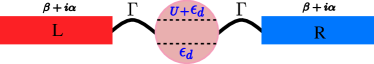
Figure 1: Schematic representation of an SET, a correlated QD, with $\epsilon_{d}$ and $\epsilon_{d}+U$ energy levels, and Coulomb repulsion $U$. The QD is symmetrically coupled, with strength $\Gamma$, to left and right uncorrelated conducting leads. The one-dimensional leads are subjected to Rashba ($\alpha$) and Dresselhaus ($\beta$) SOC.

The SET studied in this work is represented schematically in Fig. 1. It is constituted by a correlated QD immersed into one-dimensional (1D) conducting leads that exhibit both Rashba [66] and Dresselhaus [67] SOC. The total Hamiltonian is given by $H=H_{leads}+H_{QD}+H_{hyb}$, where

$$H_{leads} = -2t\sum_{k\sigma s}[cos(ka)-\mu]c^{\dagger}_{k\sigma,s}c_{k\sigma,s}$$ (1)

$$- 2\sum_{ks}\sin(ka)(\gamma c_{k\uparrow,s}^{\dagger}c_{k\downarrow,s}+h.c.),$$

$$H_{QD}=\sum_{\sigma}\epsilon_{d}n_{d\sigma}+Un_{d\uparrow}n_{d\downarrow},$$ (2)

$$H_{hyb}=\sum_{k\sigma s}V_{k\sigma,s}(c_{k\sigma,s}^{\dagger}d_{\sigma}+d_{\sigma}^{\dagger}c_{k\sigma,s}).$$ (3)

In the equations above, $c_{k\sigma,s}^{\dagger}$ ($c_{k\sigma,s}$) creates (annihilates) an electron with momentum $k$ and spin $\sigma=\uparrow,\downarrow$ in the $s=L,R$ lead, while $d_{\sigma}^{\dagger}$ ($d_{\sigma}$) creates (annihilates) an electron with spin $\sigma=\uparrow,\downarrow$ in the QD, being $n_{d}=d_{\sigma}^{\dagger}d_{\sigma}$ the number operator for the $\epsilon_{d}$ QD active level. More specifically, $H_{leads}$ represents the leads, modeled by a 1D tight-binding approximation with nearest-neighbor hopping $t$, lattice parameter $a=1$, and chemical potential $\mu$. Rashba ($\alpha$) and Dresselhaus ($\beta$) SOC parameters are taken into account through $\gamma=\beta+i\alpha$. $H_{QD}$ describes the QD, characterized by a localized bare level $\epsilon_{d}$ and a local Coulomb repulsion $U$, while $H_{hyb}$ accounts for the hybridization between electrons in the leads and the QD. In the following, we consider that the matrix elements of the hybridization $V_{k\sigma,s}$, originating from the coupling between the conducting leads and the QD electron’s wave function, are $k$-, spin-, and lead-independent, i.e., $V_{k\sigma,s}=V$. Finally, we assume that $\epsilon_{d}$ can be varied by application of a voltage to a metallic back gate.

As shown in previous works [56, 57, 58, 59, 60, 61, 62, 63, 64, 65], the inclusion of SOC in the conduction band results in a broken spin SU(2) symmetry. We may define a helicity operator $\hat{h}$ with eigenstates $|k\nu\rangle$, such that $[\hat{h},H_{leads}]=0$. However, unfortunately, $\nu=\pm 1$ is not a good quantum number of the whole system (leads+QD), because the helicity is not defined for the QD. Thus, it is convenient, in 1D, to make a spin rotation to partially recover the SU(2) symmetry [65]. Therefore, we choose a new spin basis $S_{r}$, in which both the impurity and the conduction spins are projected along an axis $\hat{r}$ that points along the SOC effective magnetic field, whose orientation depends on the SOC parameter $\gamma$ [65]. The basis transformations for impurity and SOC conduction band are $d^{\dagger}_{\sigma_{r}}=\nicefrac{{1}}{{2}}(d^{\dagger}_{\uparrow}+\sigma_{r}e^{i\phi}d^{\dagger}_{\downarrow})$ and $c^{\dagger}_{k\sigma_{r}}=\nicefrac{{1}}{{2}}(c^{\dagger}_{k\uparrow}+\sigma_{r}e^{i\phi}c^{\dagger}_{k\downarrow})$, respectively, where $\sigma_{r}=\pm$ indicates spins $\uparrow$ ($+$) and $\downarrow$ ($-$) along the $\hat{r}$ direction. In addition, $\phi=\nicefrac{{\alpha}}{{\beta}}$. In this new basis, the Hamiltonian can be rewritten as

$$H = \sum_{k,\sigma_{r}}\epsilon_{k\sigma_{r}}c_{k\sigma_{r}}^{\dagger}c_{k\sigma_{r}}$$ (4)

$$+ \sum_{\sigma_{r}}\epsilon_{d}n_{d\sigma_{r}}+Un_{d\uparrow_{r}}n_{d\downarrow_{r}}$$

$$+ \sum_{k,\sigma_{r}}V\left(c_{k\sigma_{r}}^{\dagger}d_{\sigma_{r}}+d_{\sigma_{r}}^{\dagger}c_{k\sigma_{r}}\right),$$

where $n_{d\sigma_{r}}=d_{\sigma_{r}}^{\dagger}d_{\sigma_{r}}$ is the QD number operator, $c_{k\sigma_{r}}^{\dagger}(c_{k\sigma_{r}})$ creates (annihilates) an electron in the Fermi sea with momentum $k$ and spin $\sigma_{r}$. Note that we have removed the $s=L,R$ subindex, since we are assuming that the QD couples only to the symmetric combination of the $L$ and $R$ leads. Finally, the dispersion relation $\epsilon_{k\sigma_{r}}$ is given by

$$\epsilon_{k\sigma_{r}}=-2\sqrt{t^{2}+|\gamma|^{2}}\cos\left(k-\sigma_{r}\varphi\right)+\mu,$$ (5)

where $\varphi=\tan^{-1}\nicefrac{{|\gamma|}}{{t}}$. As shown in Ref. [65], in 1D the SOC influence over the Kondo effect is to cause a renormalization of the zero-SOC half-bandwidth $D$ and the QD-band hybridization, at the Fermi energy, $\Gamma=\Delta(0)$, to new $\gamma$-dependent values ${D}_{\gamma}=2\sqrt{t^{2}+|\gamma|^{2}}$ [68] and

$${\Gamma}_{\gamma}={\Delta}_{\gamma}(0)=\frac{V^{2}}{2\sqrt{t^{2}+|\gamma|^{2}}}.$$ (6)

Thus, the renormalized finite-SOC SIAM Kondo temperature ${T}_{K\gamma}$, in the wide-band limit, can be written as [65]

$${T}_{K\gamma}=0.364\left(\frac{2{\Gamma}_{\gamma}U}{\pi}\right)^{\frac{1}{2}}\exp\left[\frac{\pi\epsilon_{d}\left(\epsilon_{d}+U\right)}{2{\Gamma}_{\gamma}U}\right].$$ (7)

On the other hand, Friedel’s sum rule [69] gives a relationship, at $T=0$, between the extra state (induced below the Fermi level by a scattering center) and the phase shift at the chemical potential $\eta_{\sigma}(\mu)$, obtained by the transference matrix $T_{d,k\sigma_{r}}(z)=V_{k}^{2}G_{d,k\sigma_{r}}^{imp}(z)$, where $V_{k}$ is the scattering potential. For the SIAM, the extra states induced are given by the occupation number $n_{d,\sigma_{r}}$ of the QD localized state, and the scattering potential is the hybridization that affects the conduction electrons. Thus, Friedel’s sum rule for the SIAM can be written as [70]

$$\rho_{d\sigma}(\mu)=\frac{sin^{2}\left(\nicefrac{{\pi n_{d\sigma}}}{{2}}\right)}{{\Gamma}_{\gamma}\pi},$$ (8)

where $\rho_{d\sigma}(\mu)$ is the LDOS of the QD level at the chemical potential. In the Kondo regime, Eq. (8) implies that a suppression of ${\Gamma_{\gamma}}$ leads to an enhancement of the so-called Kondo peak at the chemical potential and the consequent suppression of ${T}_{K\gamma}$, due to the concomitant narrowing of the Kondo peak. Since SOC suppresses ${\Gamma_{\gamma}}$ [see Eq.(6)], it results that SOC suppresses ${T}_{K\gamma}$ [this can also be concluded from Eq. (7)].

To perform the NRG calculations, we use the open-source NRG code NRG-Ljubljana [71]. The NRG parameters used were $\Lambda=2$, Wilson chain length $68$, keeping 20000 states. In addition, for all our calculations we use a zero-SOC hybridization function at the Fermi level ${\Gamma}_{0}=0.007$ [72].

III Thermoelectric properties

To calculate the TE transport properties of a QD in a steady-state condition, we apply a small external bias voltage $\Delta V=V_{L}-V_{R}$ and a small temperature difference $\Delta T=T_{L}-T_{R}$ between the left (hot) and the right (cold) leads. In linear response theory, a current $J_{\alpha}$ will flow through the system under the action of a temperature gradient $\vec{\nabla}T$ and/or an electric field $\vec{E}=-\vec{\nabla}V$, where $\alpha=e$ indicates a charge current $J_{e}$, while $\alpha=Q$ indicates a heat current $J_{Q}$. The TE properties calculations follow standard textbooks [73, 74]. The electrical and thermal conductances, $G(T)$ and $K_{e}(T)$, respectively, as well as the thermopower $S(T)$ (Seebeck coefficient) are given by [75]

$$G(T)=-\lim_{\Delta V\rightarrow 0}\left(J_{e}/\Delta V\right)_{\mid_{\Delta T=0}}=e^{2}\mathcal{L}_{0}(T),$$ (9)

$$K_{e}(T) = -\lim_{\Delta T\rightarrow 0}\left(J_{Q}/\Delta T\right)_{\mid_{J_{e}=0}}$$

$$= \frac{1}{T}\left(\mathcal{L}_{2}(T)-\frac{\mathcal{L}_{1}^{2}(T)}{\mathcal{L}_{0}(T)}\right),$$

$$S(T)=\lim_{\Delta T\rightarrow 0}\left(\Delta V/\Delta T\right)_{\mid_{J_{e}=0}}=\left(\frac{-1}{eT}\right)\frac{\mathcal{L}_{1}(T)}{\mathcal{L}_{0}(T)},$$ (11)

where, to calculate the transport coefficients $\mathcal{L}_{0}(T)$, $\mathcal{L}_{1}(T)$, and $\mathcal{L}_{2}(T)$, we follow Ref. [76], where expressions for the particle current and thermal flux, for a QD, were derived within the framework of Keldysh non-equilibrium Green’s functions. Thus, the TE transport coefficients were obtained in the presence of temperature and voltage gradients, with the Onsager relations automatically satisfied, in the linear regime. The TE transport coefficients (for $n=0,1,2$) consistent with the general TE formulas derived above are given by

$$\mathcal{L}_{n}(T)=\frac{2}{h}\int{\left(-\frac{\partial f(\omega,T)}{\partial\omega}\right)\omega^{n}\tau(\omega,T)d\omega},$$ (12)

where $\tau(\omega,T)$ is the transmittance for electrons with energy $\epsilon=\hbar\omega$ and temperature $T$, while $f(\omega,T)$ is the Fermi-Dirac distribution function.

For ordinary metals, the Wiedemann-Franz law states that the ratio between the electronic contribution to the thermal conductance $K_{e}(T)$ and the product of temperature $T$ and electrical conductance $G(T)$,

$$L=\frac{K_{e}(T)}{TG(T)},$$ (13)

is independent of temperature and takes a universal value given by the Lorenz number $L_{o}=(\nicefrac{{\pi^{2}}}{{3}})(\nicefrac{{k_{B}}}{{e}})^{2}$, where $k_{B}$ is the Boltzmann constant and $-e$ is the electron charge. Note that, in the calculations that follow, we present the Wiedemann-Franz law in units of $L_{o}$,

$$WF=\frac{L}{L_{o}},$$ (14)

so that it is easy to spot deviations from what is expected for ordinary metals, i.e., $WF=1$.

The dimensionless TE figure of merit $ZT$, which measures the efficiency of materials or devices to be employed as thermopower generators or cooling systems, is defined by

$$ZT=S^{2}TG(T)/K_{e}(T).$$ (15)

In ordinary metals, both $G(T)$ and $K_{e}(T)$ are related to the same electronic scattering processes, with only weak energy dependence, and satisfying the Wiedemann-Franz law, which is the main reason why metals show lower $ZT$ values. The conditions that a device must fulfill to produce a high $ZT$ value were discussed in Ref. [77], where the authors showed that a narrow energy distribution of the carriers was needed to produce a large value of $ZT$.

Employing Eqs. (13) to (15), we can write $ZT$ as a function of the thermopower $S$ and the Wiedemann-Franz law $WF$ [expressed in units of $L_{o}$, as in Eq. (14)]

$$ZT=\frac{S^{2}}{WF}.$$ (16)

This equation shows that violations of the Wiedemann-Franz law can lead to an effective increase of $ZT$ in regions where $WF<1$, as long as there is no concomitant decrease in the thermopower $S$.

The behavior of the TE coefficients is governed by the transmittance $\tau(\omega,T)$ [see Eq. (12)]. For a QD in an immersed (or embedded) geometry, it can be written in terms of the QD Green’s function as

$$\tau(\omega,T)=\Gamma\Im[G_{d}(\omega,T)],$$ (17)

where ${\Gamma}_{\gamma}=\pi V^{2}\rho^{c}(\mu)$, with $\rho^{c}_{\sigma_{r}}(\mu)$ being the spin-orbit dependent leads’ DOS at the Fermi energy, and $\Im$ indicates the imaginary part.

IV Spin-orbit effects over the density of states

In Kondo physics, the hybridization function at the Fermi energy, ${\Gamma}_{\gamma}$, is an important quantity. In all the calculations that follow, we employed ${\Gamma}_{0}=0.007$ [72], in units of ${D}_{0}$, which is the half-width of the conduction band in the absence of SOC [68], and the chemical potential is always located at $\mu=0$. In addition, we will vary SOC in the interval $0.0\leq|\gamma|\leq 0.5$, which will make $\Gamma_{\gamma}$ vary in accordance with Eq. (6).

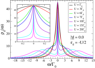
Figure 2: QD’s LDOS $\rho_{d}(\omega)$ for different values of the electronic correlation $U$ and $|\gamma|=0.0$, showing the formation of the Kondo peak, starting from $U=\Gamma_{0}$, when the system is inside the intermediate valence regime, to $U=20.0\Gamma_{0}$, when the system is deep inside the Kondo regime. Inset: Details of the formation of the Kondo peak. Note that all curves are at the PHS point $\epsilon_{d}=\nicefrac{{-U}}{{2}}$.

In Fig. 2, we show the QD’s LDOS $\rho_{d}(\omega)$ at the particle-hole symmetric (PHS) point ($\epsilon_{d}=-U/2$) of the SIAM for several different values of the Coulomb repulsion $\Gamma_{0}\leq U\leq 20.0\Gamma_{0}$, and for vanishing SOC, $|\gamma|=0.0$. For this range of variation of $\nicefrac{{U}}{{\Gamma_{0}}}$, it is well know that the system passes from an intermediate valence regime (for the smaller values of $\nicefrac{{U}}{{\Gamma_{0}}}$) to the Kondo regime (for the larger values of $\nicefrac{{U}}{{\Gamma_{0}}}$). The passage from the former to the latter is a crossover, thus it does not occur for an specific value of $\nicefrac{{U}}{{\Gamma_{0}}}$. Nonetheless, the results show the gradual formation of the Kondo peak as the correlation $U$ is varied from $U=\Gamma_{0}$ to $U=20.0\Gamma_{0}$, where the system is already deep into the Kondo regime [very low Kondo temperature ${T}_{K\gamma}$—see Eq. (7)]. For $U=\Gamma_{0}$, we have a broad peak centered around the chemical potential, located in $\omega=0$ (black curve); in addition, the two symmetric Hubbard satellite peaks characteristic of the PHS point cannot be discerned. However, as we increase the correlation to $U=10.0\Gamma_{0}$ (purple curve), the Hubbard satellites are already well established, but the Kondo peak is only completely formed above $U=15.0\Gamma_{0}$ (cyan curve). In the inset, the formation of the Kondo peak, as the electronic correlation increases, is shown more clearly. Along this process, the peak diminishes its width, indicating the establishment of the Kondo regime characterized by a Kondo temperature $T_{K\gamma}$, which is proportional to the width of the Kondo peak, thus, the narrower the peak, the lower is the Kondo temperature and the deeper is the system into the Kondo regime.

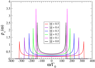
Figure 3: Density of states of the 1D conducting leads $\rho_{c}(\omega)$ for different values of SOC, $0.0\leq|\gamma|\leq 0.5$. Notice the sizable broadening of the band, as well as the decrease of the DOS at the Fermi energy.

In Fig. 3, we show the DOS of the conducting leads $\rho_{c}(\omega)$, corresponding to different values of SOC, $0.0\leq|\gamma|\leq 0.5$. The main effects of the SOC is to produce a broadening of the band, and, as a consequence, a decrease of the DOS at the chemical potential $\mu=0$, which, see Eq. (6), results in the decrease of the value of the SOC-renormalized hybridization function at the Fermi energy.

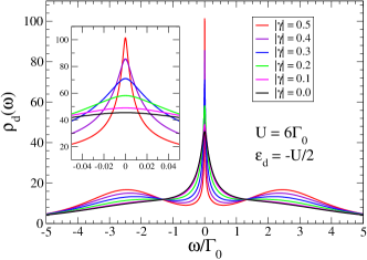
Figure 4: QD’s LDOS $\rho_{d}(\omega)$, for different SOC values, $0.0\leq|\gamma|\leq 0.5$, at the PHS point, for $U=6.0\Gamma_{0}$. Note that the black curve ($|\gamma|=0.0$) corresponds to the green curve in Fig. 2, thus inside the intermediate valence regime, clearly showing that SOC drives the system deep into the Kondo regime. Notice the very well formed Kondo peak for $|\gamma|=0.5$ (red curve). Inset: zoom close to $\omega=0$, showing details of the evolution of the Kondo peak.

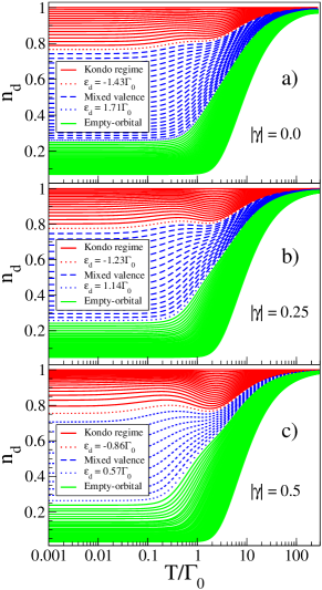
Figure 5: QD occupation-number map. Panels (a), (b) and (c), for $|\gamma|=0.0$, $0.25$, and $0.5$, respectively, indicate the temperature variation of $n_{d}$ for varying $\epsilon_{d}$ in the interval $-U/2\leq\epsilon_{d}\leq 8.71\Gamma_{0}$. The definition of the different regimes follows Ref. [21], i.e., Kondo (red), $|n_{d}-1|_{T\approx 0}\leq 0.25$, intermediate-valence (blue), $|n_{d}-0.5|_{T\approx 0}\leq 0.25$, empty-orbital (green), $|n_{d}|_{T\approx 0}\leq 0.25$. The dotted curves, with corresponding $\epsilon_{d}$ values indicated in the legends, demarcate the crossover from one regime to the next. All results for $U=7.0\Gamma_{0}$

In Fig. 4, we plot the QD’s LDOS $\rho_{d}(\omega)$, for different values of $|\gamma|$, for a PHS situation. We do all the calculations for $U=6.0\Gamma_{0}$, thus, at $|\gamma|=0.0$, not deep into the Kondo regime (see green curve in Fig. 2). However, by the evolution of $\rho_{d}(\omega)$, due to the increase of SOC from $|\gamma|=0$ to $|\gamma|=0.5$, it can be clearly seen that the increase of SOC drives the system deep into the Kondo regime. Indeed, the height of the Kondo peak increases while its width decreases, indicating a lowering of the Kondo temperature. This striking effect is directly related to the decreasing value of the SOC-renormalized hybridization function at the Fermi level, since, according to Friedel’s sum rule [Eq. (8)], this should cause an increase of $\rho_{d}(\mu=0)$ and, according to Eq. (7), a decrease of the Kondo temperature, with an accompanying reduction of the Kondo-peak half-width. It is also possible to discern a slight increase in the separation between the satellite Hubbard peaks, pointing to an increase of the effective Hubbard on-site repulsion, which accounts for an increase in the electronic correlations.

V Thermoelectric properties maps

In this section, we plot the TE properties for different values of $\epsilon_{d}$, from the Kondo to the empty-orbital regime, as a function of $T/\Gamma_{0}$, for different values of SOC, $|\gamma|=0.0$, $0.25$, and $0.5$. For all the results in this section, we consider the electronic correlation $U=7.0\Gamma_{0}$, and, to characterize the different regimes of the system (at low temperature), we follow the definitions in Ref. [21], viz., (i) $n_{d}$ values in the interval $|n_{d}-1|_{T\approx 0}\leq 0.25$ (red curves) correspond to the Kondo regime, (ii) $|n_{d}-0.5|_{T\approx 0}\leq 0.25$ (blue curves) correspond to the mixed-valence regime, (iii) $|n_{d}|_{T\approx 0}\leq 0.25$ (green curves) correspond to the empty-orbital regime. The borders between different regimes occur as crossovers. Although these regime definitions are more appropriate to the low temperature region, we extend them to the higher temperature regions as well.

In panels (a), (b), and (c) of Fig. 5, we plot the QD occupation number $n_{d}$ as a function of temperature for different values of $\epsilon_{d}$ ($-U/2\leq\epsilon_{d}\leq 8.71\Gamma_{0}$). Panels (a), (b), and (c) are for $|\gamma|=0.0$, $0.25$ and $0.5$, respectively. The $\epsilon_{d}$ values shown in the legend represent the values at which, according to the definitions above, there is a crossover between different regimes, indicated by dotted curves. By comparing different panels, it is clear that SOC affects the overall spread of each region. Indeed, as $|\gamma|$ increases from $0.0$ to $0.5$, the empty-orbital and Kondo regions expand, at the expense of the mixed-valence region. This makes sense, as the decrease of the hybridization between the QD and the conduction band, caused by SOC, should enhance spin fluctuations (enhancing Kondo and empty-orbital) at the expense of charge fluctuations (weakening intermediate valence). As we shall see next, this will be reflected in the results for the TE properties.

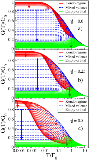
Figure 6: Same parameters as in Fig. 5, but now showing the electrical conductance $G(T)$ (in units of the quantum of conductance $G_{0}$) as a function of temperature. The arrows indicate the direction of increasing values of $\epsilon_{d}$, where the values of $\epsilon_{d}$ for each curve are the same as in Fig. 5. The temperature is in units of $\Gamma_{0}$ and $U=7.0\Gamma_{0}$.

In panels (a), (b), and (c) in Fig. 6, we have similar plots to the ones in Fig. 5, but this time for the electrical conductance $\nicefrac{{G(T)}}{{G_{0}}}$, as a function of temperature, where $G_{0}=\nicefrac{{2e^{2}}}{{h}}$ is the quantum of conductance (taking spin into account). The arrows indicate the direction of increasing values of $\epsilon_{d}$, where the values of $\epsilon_{d}$ for each curve are the same as in Fig. 5. Following Ref. [78], the Kondo temperature, $T_{K\gamma}$, can be calculated, from each curve in all three panels, by computing the temperature value where the electrical conductance attains $G(T_{K\gamma})=\nicefrac{{G_{0}}}{{2}}=\nicefrac{{e^{2}}}{{h}}$. By using that criterion to define $T_{K\gamma}$, it is easy to see that the average $T_{K\gamma}$ of the red curves (Kondo regime, as defined by Costi et al. [21]) in panel (c) is more than an order of magnitude lower than the average $T_{K\gamma}$ in panel (a). Taking in account the universally accepted concept that, the lower is $T_{K\gamma}$, the deeper we are into the Kondo regime, leads us to assert that an increase in SOC drives the SIAM deeper into the Kondo regime, as already observed through the LDOS results in Fig. 4.

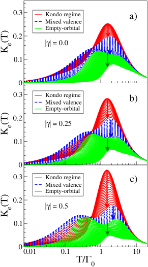
Figure 7: Same parameters as in Figs. 5 and 6, but now showing the electronic contribution to the thermal conductance $K_{e}(T)$ as a function of temperature, in units of $\Gamma_{0}$. The arrows indicate the direction of increasing values of $\epsilon_{d}$.

In panels (a), (b), and (c) of Fig. 7, we have similar plots to the ones in Figs. 5 and 6, but this time for the thermal conductance $K_{e}$, as a function of temperature, in units of $\Gamma_{0}$. The arrows have the same meaning as in Fig. 6. Comparing the three panels in Fig. 7, we observe again the SOC’s tendency to reduce the intermediate valence region and to increase the Kondo and the empty-orbital regions. All three panels (a), (b), and (c), for $|\gamma|=0.0$, $0.25$, and $0.5$, respectively, exhibit a crossing point, slightly below $T=\Gamma_{0}$ (and weakly dependent on $\gamma$). This crossing point appears as the convergence of all the red and blue curves to a very narrow window interval at $T\approx\Gamma_{0}$ [21]. It is interesting to note that the width of this window becomes increasingly narrower as $\gamma$ increases, basically collapsing to a single point for $|\gamma|=0.5$. These crossing points are characteristic signatures of strongly correlated systems, like it was observed for the specific heat in the Hubbard model in Ref. [79].

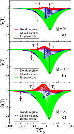
Figure 8: Same parameters as in Figs. 5, 6 and 7, but now showing the thermopower $S(T)$ as a function of temperature. Notice the sizable change in the interval of variation of S(T) (increase in the maximum and minimum values) as a function of $\gamma$. This will be relevant to the TE figure of merit results in Fig. 15. Again, the arrows indicate the direction of increasing values of $\epsilon_{d}$.

In panels (a), (b), and (c) of Fig. 8, we show plots similar to the ones in Figs. 5, 6, and 7, but this time for the thermopower $S$, as a function of temperature. There are three peaks in the Kondo regime (red curves), viz., two minima satellite peaks located at left and right of a maximum central peak located at $T\approx\Gamma_{0}$, which is inside the interval $[T_{1}:T_{2}]$. Temperatures $T_{1}$ and $T_{2}$ represent energy scales associated to the Kondo regime that characterize the changes in who are the $S(T)$ heat carriers, from electrons to holes to electrons, from left to right. In the PHS point, i.e., $\epsilon_{d}=\nicefrac{{-U}}{{2}}$, $S(T)=0$, however, away from the PHS point, $S(T)$ acquires a temperature dependence. Comparing the three panels, for $|\gamma|=0.0$, $0.25$ and $0.5$, when the system is not in the PHS point, there is a strong increase in the height of the maximum Kondo-related peak (red curves) and in the depth of the minimum empty-orbital-related peak (green curves), as $|\gamma|$ increases from $0.0$ to $0.5$, which is the most striking characteristic of the thermopower shown here. That will contribute to the sizable $ZT$ increase seen in Fig. 15(c), at finite $\gamma$, when compared to zero-SOC [Fig. 15(a)].

VI Universality under SOC

In this section, we present a study of the universal behavior of the electrical and thermal conductances, as well as of the thermopower, as a function of temperature, for different values of $\epsilon_{d}$, for $|\gamma|=0$, and how this universal behavior changes for varying SOC.

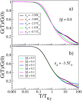
Figure 9: (a) Universal behavior of the electrical conductance $\nicefrac{{G(T)}}{{G(0)}}$ for different values of $\epsilon_{d}$ and $|\gamma|=0.0$ as a function of the scaled temperature $\nicefrac{{T}}{{T_{k\gamma}}}$. The universality occurs inside the Kondo regime, since the magenta curve, which does not collapse, falls already inside the intermediate valence regime. (b) Universal behavior of $\nicefrac{{G(T)}}{{G(0)}}$, as a function of the scaled temperature $\nicefrac{{T}}{{T_{K\gamma}}}$, where all curves for different SOC ($0.0\leq|\gamma|\leq 0.5$) collapse into a single curve $f(T/T_{K\gamma})$ for temperatures up to $T\gtrsim T_{K\gamma}$.

In Fig. 9(a), we plot the electrical conductance $\nicefrac{{G(T)}}{{G(0)}}$ as a function of the scaled temperature $\nicefrac{{T}}{{T_{K\gamma}}}$, for several $\epsilon_{d}$ values, for $|\gamma|=0.0$i, where $G(0)$ is given by Eq. (10) in Ref. [21]. As expected, the curves for the first four values of $\epsilon_{d}$, which fall inside the Kondo regime, collapse into a single curve. On the other hand, the cyan curve, for $\epsilon_{d}=-0.71\Gamma_{0}$, which is inside the intermediate valence regime [see Fig. 5(a)], does not collapse into the other curves. The situation is similar if we stay at the PHS point and vary $\gamma$. In Fig. 9(b) we plot $\nicefrac{{G(T)}}{{G(0)}}$ in the PHS point, $\epsilon_{d}=\nicefrac{{-U}}{{2}}$, as a function of the scaled temperature $\nicefrac{{T}}{{T_{K\gamma}}}$, for different values of SOC, $0.0\leq|\gamma|\leq 0.5$. In the Kondo regime, the electrical conductance presents a universal character: $\nicefrac{{G(T)}}{{G(0)}}=f(\nicefrac{{T}}{{T_{K\gamma}}})$, with a functional form that is independent of SOC. Note that the larger is $|\gamma|$, the further above $T_{K\gamma}$ remains the invariance of $f(\nicefrac{{T}}{{T_{K\gamma}}})$ with $\gamma$.

We just saw that a quite interesting characteristic of electronic transport through QDs is the universal behavior in the Kondo regime when the temperature is scaled by a characteristic temperature, such as $T_{K\gamma}$ for $G(T)$, as just shown above, or by $T^{\theta}_{K\gamma}$ for $K_{e}(T)$. The temperature $T^{\theta}_{K\gamma}$ is the equivalent of $T_{K\gamma}$ for $K_{e}(T)$ and can be computed using the Wiedemann-Franz law, Eq. (13), $\nicefrac{{K_{e}}}{{T}}\approx L_{o}\times WF\times G(T)$, being defined by the relation [21]

$$\frac{K_{e}(T=T_{K\gamma}^{\theta})}{T^{\theta}_{K\gamma}}=\frac{\alpha}{2},$$ (18)

where $\alpha$ is obtained through

$$\alpha=\lim_{T\rightarrow 0}\frac{K_{e}(T)}{T}.$$ (19)

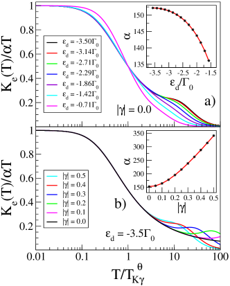
Figure 10: (a) Universal behavior of the thermal conductance $\nicefrac{{K_{e}(T)}}{{\alpha T}}$ as a function of the scaled temperature $\nicefrac{{T}}{{T^{\theta}_{K\gamma}}}$, for several values of $\epsilon_{d}$ (inside the Kondo regime), for $|\gamma|=0.0$. The single curve inside the intermediate valence regime ($\epsilon_{d}=-0.71\Gamma_{0}$, magenta curve) does not collapse into the Kondo regime universality function. (b) Universal behavior of $\nicefrac{{K_{e}(T)}}{{\alpha T}}$, as a function of the scaled temperature $\nicefrac{{T}}{{T^{\theta}_{K\gamma}}}$, where all curves for different SOC ($0.0\leq|\gamma|\leq 0.5$) collapse into a single curve $g(T/T^{\theta}_{K\gamma})$. In both insets we show the values of $\alpha$ that produce the collapse.

In Fig. 10(a), we plot the thermal conductance $\nicefrac{{K_{e}(T)}}{{\alpha T}}$ as a function of the scaled temperature $\nicefrac{{T}}{{T^{\theta}_{K\gamma}}}$, for several $\nicefrac{{-U}}{{2}}\leq\epsilon_{d}\leq-0.71\Gamma_{0}$ and $|\gamma|=0.0$. In the inset to panel (a), we plot the rescaling parameter $\alpha$ as a function of $\epsilon_{d}$, in $\Gamma_{0}$ units. It is clear from the results that the rescaling by $T^{\theta}_{K\gamma}$ and $\alpha$ collapses all the $K_{e}(T)$ curves, for different $\epsilon_{d}$, for $T\lesssim T^{\theta}_{K\gamma}$, onto a single universal curve. The exception, as in the case of the electric conductance, was for $\epsilon_{d}=-0.71$ (magenta curve), which is inside the intermediate valence regime. In Fig. 10(b) we plot $\nicefrac{{K_{e}(T)}}{{\alpha T}}$ at the PHS point, for different values of $|\gamma|$. In the Kondo regime, the thermal conductance thus presents a universal character: $\nicefrac{{K_{e}(T)}}{{\alpha T}}=g(\nicefrac{{T}}{{T^{\theta}_{K\gamma}}})$, showing its invariance with SOC. In addition, in the PHS point, the thermal conductance obeys, by construction [see Eqs. (18) and (19)], $\nicefrac{{K_{e}(T)}}{{\alpha T}}=1.0$, at low temperatures. In the inset to panel (b), we plot the rescaling parameter $\alpha$ as a function of $|\gamma|$.

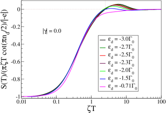
Figure 11: Temperature dependence of the thermopower $S(T)$, plotted in units of $\nicefrac{{\pi\zeta T\cot(\nicefrac{{\pi n_{d}}}{{2}})}}{{e}}$ for $-3.0\Gamma_{0}\leq\epsilon_{d}\leq-0.71\Gamma_{0}$ and $|\gamma|=0.0$. Universality is achieved for $T\lesssim\zeta T$. As it happened for the electric and thermal conductances, the curve for the first value inside the intermediate valence regime ($\epsilon_{d}=-0.71$, magenta curve) does not collapse into the universal curve.

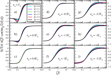
Figure 12: (a) to (i): Comparison of thermopower universality in the Kondo and intermediate valence regimes. Each panel contains the scaled thermopower (for $0.0\leq|\gamma|\leq 0.5$) for different values of $\epsilon_{d}$. Notice how the universality is more complete in the intermediate valence regime. Indeed, panels (c) and (d), for $\epsilon_{d}=0.0\Gamma_{0}$ and $-0.5\Gamma_{0}$, present the more complete collapse of the thermopower results for different values of $\gamma$. These two values of $\epsilon_{d}$ are deep into the intermediate valence regime, for all values of $\gamma$ [see Fig. 5(c)].

As pointed out by Costi et al. [21], in the Fermi liquid regime [80], $\nicefrac{{S(T)}}{{T}}$, for a range of different values of $\epsilon_{d}$ in the Kondo regime, scales as

$$\frac{S(T)}{T}=-\frac{\pi\zeta}{e}\cot(\frac{\pi n_{d}}{2}),$$ (20)

where $-e$ is the electron charge, and the factor $\zeta$ can be obtained from the numerical value of $\lim_{T\rightarrow 0}|S(T)/T|$ and the occupation number $n_{d}$.

As done for the electric and thermal conductances (Figs. 9 and 10), we will employ this procedure to rescale the temperature dependence of $S(T)$ to check the universality for varying $\epsilon_{d}$ (at $|\gamma|=0.0$) and for varying $\gamma$ at fixed $\epsilon_{d}$. In Fig. 11, we plot the thermopower $S(T)$, in units of $\nicefrac{{\pi\zeta T\cot(\nicefrac{{\pi n_{d}}}{{2}})}}{{e}}$, as a function of the scaled temperature $\zeta T$, for several $\epsilon_{d}$ and $|\gamma|=0.0$. In agreement with what we obtained for the electric and thermal conductances, $S(T)$ attains universality if we stay inside the Kondo regime, i.e., $-3.0\Gamma_{0}\leq\epsilon_{d}\leq-1.5\Gamma_{0}$. For $\epsilon_{d}=-0.71$ (magenta curve) the universality is lost. In addition, since the sign of $S(T)$ is determined by the charge of the heat carriers ($S(T)>0\leftrightarrow$ holes, and $S(T)<0\leftrightarrow$ electrons), for temperatures below $\zeta T\simeq 2.0$ (see black dotted lines in Fig. 11), the carriers are electrons, and, in a region above $\zeta T\simeq 2.0$ the carriers are holes. In the limit of high temperatures, $S(T)\rightarrow 0$.

Something curious, however, occurs when we analyze the universality at fixed $\epsilon_{d}$ and $0.0\leq|\gamma|\leq 0.5$. As shown in Fig. 12, where panels (a) to (i) show the scaling of $S(T)$ for different values of $\epsilon_{d}$ in the interval $-3.2\Gamma_{0}\leq\epsilon_{d}\leq\Gamma_{0}$ (spanning the Kondo and intermediate valence regimes), the universality is achieved only deep into the intermediate valence regime (panels (c) and (d), for $\epsilon_{d}=-0.5\Gamma_{0}$ and $0.0\Gamma_{0}$, respectively). This is in contrast to what was observed for the electric and thermal conductances [Figs. 9(b) and 10(b)], where the universality was observed inside the Kondo regime.

In Fig. 13, we re-plot Fig. 12(d) ($S(T)$ for $\epsilon_{d}=-0.5\Gamma_{0}$) to study the variation of $T_{K\gamma}$ with $\gamma$ (top inset), the dependence of the Fermi liquid parameter $\zeta$ with $\gamma$ (bottom-left inset), and the dependence of the QD occupancy $n_{d}$ with $\gamma$ (bottom-right inset). As expected, since the increase in $\gamma$ moves the system in the Kondo regime direction, we see that there is a non-monotonic increase in $n_{d}$ as $\gamma$ increases (bottom-right inset), while, as expected too, $T_{K}$ decreases with $\gamma$ (top inset). In addition, there is a corresponding increase in $\zeta$ with $\gamma$ (bottom-left inset).

Thus, we have analyzed two types of universalities for the quantities $G(T)$, $K_{e}(T)$, and $S(T)$: (i) zero-SOC and varying $\epsilon_{d}$, for which we found that there is universality for $G(T)$, $K_{e}(T)$, and $S(T)$ in the Kondo regime [see Figs. 9(a), 10(a), and 11]; (ii) fixed $\epsilon_{d}$ and varying $\gamma$, for which both $G(T)$ and $K_{e}(T)$ show universality in the Kondo regime [see Figs. 9(b) and 10(b)], while, unexpectedly, $S(T)$ shows universality in the intermediate valence regime (Fig. 12). We are not completely sure why this is so.

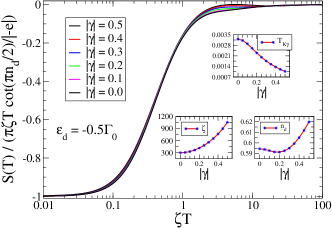
Figure 13: Same as in Fig. 11, but for $0.0\leq|\gamma|\leq 0.5$ and $\epsilon_{d}=-0.5\Gamma_{0}$. Top inset: $T_{K\gamma}$ as a function of $\gamma$; bottom-left inset: $\zeta$ as a function of $\gamma$; bottom-right inset: QD occupation $n_{d}$ as a function of $\gamma$.

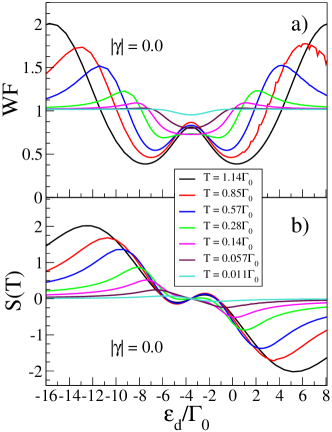
Figure 14: (a) Wiedemann-Franz law (in units of the Lorenz number, $L_{o}$) and (b) Thermopower, as a function of $\epsilon_{d}$, for several values of temperature (in units of $\Gamma_{0}$), for $U=7.0\Gamma_{0}$ and $|\gamma|=0.0$.

In panels (a) and (b) in Fig. 14, we show the Wiedemann-Franz law, in units of the Lorenz number $L_{o}$, and the thermopower, respectively, as a function of $\epsilon_{d}$ (in units of $\Gamma_{0}$), at various temperature values (also in units of $\Gamma_{0}$), for $|\gamma|=0$ and $U=7.0\Gamma_{0}$. At the lowest temperature ($T=0.011\Gamma_{0}$, cyan curve), the Wiedemann-Franz law is satisfied, aside from a small region around the PHS point ($\epsilon_{d}=-3.5\Gamma_{0}$), where $WF\lesssim 1$. As the temperature increases, the width of this region increases, as well as the departure of $WF$ from $1$. In addition, two broad peaks appear farther away from the PHS point (on the left and right of it), whose violation of the Wiedemann-Franz law (now, $WF>1$) becomes more severe, as the temperature increases. In addition, the maxima of the left and right peaks gradually move away from the PHS point with increasing temperature.

A somewhat similar picture describes the results for $S(T)$ in Fig. 14(b), with the difference that now S(T) is odd in relation to the PHS point. In addition, left and right broad peaks emerge away from the PHS point, similarly located and with similar temperature dependence as the ones shown for $WF$ in Fig. 14(a). As a consequence, given that $ZT=\nicefrac{{S^{2}}}{{WF}}$, and since $S\gtrsim WF$ at and around those broad peaks, this determines the relatively high values attained by $ZT$ in the peaks region, as shown in Fig. 15(a), for $|\gamma|=0.0$ and several temperatures.

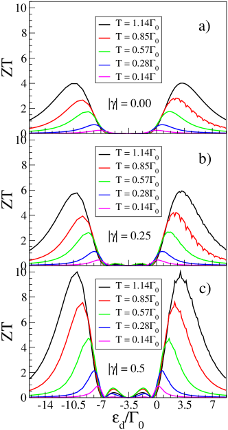
Figure 15: Dimensionless TE figure o merit $ZT$ as a function of $\epsilon_{d}$, for several values of temperature (in units of ${\Gamma_{0}}$) and $U=7.0\Gamma_{0}$. Panels (a), (b), and (c) are for $|\gamma|=0.0$, $0.25$, and $0.5$, respectively.

In panels (b) and (c) in Fig. 15, we show the dimensionless TE figure of merit $ZT$ as a function of $\epsilon_{d}$, at various temperatures, for finite SOC, $|\gamma|=0.25$ and $0.5$, respectively. When compared to Fig. 15(a), for $|\gamma|=0.0$, we observe a sizable enhancement of $ZT$ with SOC, which results from the increase of $S(T)$ with SOC, as indicated in the $S(T)$ maps in Fig. 8. We notice that, compared to the $|\gamma|=0.0$ maximum $ZT\approx 4.0$ results in Fig. 15(a) ($T=1.14\Gamma_{0}$), the $ZT\approx 10.0$ obtained for $|\gamma|=0.5$, for the same temperature, represents an improvement in ZT of $\approx 2.5$ times.

Finally, we should note that, as previously mentioned, in the calculation of these $ZT$ results, we do not consider any phononic contribution, which tends to compete with the electronic contribution to decrease the $ZT$ values as the temperature is increased. However, note that we kept the maximum temperature studied at a low enough value that justifies the neglect of phonons.

VII Conclusions and perspectives

In summary, we have studied the effect of 1D conduction band SOC over the TE transport properties of an SET. This was done, using NRG, through the calculation of temperature maps of the TE properties. We have shown that SOC drives the system deeper into the Kondo regime. We also showed that the Kondo regime universality of thermal and electrical conductances is maintained in the presence of SOC. We also show the interesting result that $S(T)$, which is universal in the Kondo regime at zero-SOC, presents a more universal behavior (for different $\gamma$) in the intermediate valence regime, when compared to the Kondo regime. More importantly, we have shown that the large increases in the thermopower, caused by SOC (see Fig. 8), translate into notable SOC-caused enhancements of the TE figure of merit ZT (see Fig. 15) for an embedded SET coupled to 1D leads. Interesting points to consider in future research are (i) how these results would change for a side-connected SET; (ii) what is the role played by the leads dimensionality in the sizable increase of the figure of merit observed for 1D leads; (iii) the Rashba and Dresselhaus conduction band SOC results obtained here can be extended to study two-dimensional (2D) systems, like the surface states of the Kondo insulator $SmB_{6}$. Some recent experimental results point out that a combination of Rashba- and Dresselhaus-like SOC [52, 53, 54, 55] can describe the states around the $X$ point of the Brillouin zone; (iv) finally, we would like to study the TE properties of an SET embedded in a 2D electron gas at the Persistent Spin Helix point ($\alpha=\beta$) [81].

VIII Acknowledgments

We thank CAPES, CNPq and FAPERJ for the support of this work. G. B. M. acknowledges financial support from the Brazilian agency Conselho Nacional de Desenvolvimento Científico e Tecnológico (CNPq), processes 424711/2018-4, 305150/2017-0 and M. S. F. acknowledges financial support from the Brazilian agency Fundação de Amparo a Pesquisa do Estado do Rio de Janeiro, process 210 355/2018.

References

- Sánchez and López [2016] D. Sánchez and R. López, C. R. Phys. 17, 1060 (2016).
- Tritt [2002] T. Tritt, in Encyclopedia of Materials: Science and Technology, edited by K. J. Buschow, R. W. Cahn, M. C. Flemings, B. Ilschner, E. J. Kramer, S. Mahajan, and P. Veyssiere (Elsevier, Oxford, 2002) p. 1.
- Shakouri [2011] A. Shakouri, Annu. Rev. Mater. Res. 41, 399 (2011).
- Tritt [2011] T. M. Tritt, Annu. Rev. Mater. Res. 41, 433 (2011).
- He and Tritt [2017] J. He and T. M. Tritt, Science 357, 1369 (2017).
- Benenti et al. [2017] G. Benenti, G. Casati, K. Saito, and R. S. Whitney, Phys. Rep. 694, 1 (2017).
- Zoui et al. [2020] M. Zoui, S. Bentouba, J. Stocholm, and M. Bourouis, Energies 13, 3606 (2020).
- Manchon et al. [2015] A. Manchon, H. C. Koo, J. Nitta, S. Frolov, and R. Duine, Nat. Mater. 14, 871 (2015).
- Cassiano and Martins [2021] J. V. V. Cassiano and G. B. Martins, J. Phys. Condens. Matter 33, 175301 (2021).
- Xu et al. [2017] N. Xu, Y. Xu, and J. Zhu, npj Quantum Mater. 2, 51 (2017).
- Xu et al. [2020] K.-J. Xu, S.-D. Chen, Y. He, J. He, S. Tang, C. Jia, E. Yue Ma, S.-K. Mo, D. Lu, M. Hashimoto, T. P. Devereaux, and Z.-X. Shen, Proceedings of the National Academy of Sciences 117, 15409 (2020).
- Figueira, M.S. et al. [2012] Figueira, M.S., Silva-Valencia, J., and Franco, R., Eur. Phys. J. B 85, 203 (2012).
- Gooth et al. [2018] J. Gooth, G. Schierning, C. Felser, and K. Nielsch, MRS Bull. 43, 187 (2018).
- Ramos et al. [2014] E. Ramos, J. Silva-Valencia, R. Franco, and M. S. Figueira, Int. J. Thermal Sci. 86, 387 (2014).
- Bulla et al. [2008] R. Bulla, T. A. Costi, and T. Pruschke, Rev. Mod. Phys. 80, 395 (2008).
- Hewson [1993] A. C. Hewson, The Kondo Problem to Heavy Fermions (Cambridge University Press, 1993).
- Seridonio et al. [2009a] A. C. Seridonio, M. Yoshida, and L. N. Oliveira, EPL 86, 67006 (2009a).
- Yoshida et al. [2009] M. Yoshida, A. C. Seridonio, and L. N. Oliveira, Phys. Rev. B 80, 235317 (2009).
- Seridonio et al. [2009b] A. C. Seridonio, M. Yoshida, and L. N. Oliveira, Phys. Rev. B 80, 235318 (2009b).
- Oliveira et al. [2010] L. N. Oliveira, M. Yoshida, and A. C. Seridonio, J. Phys. Conf. Ser. 200, 052020 (2010).
- Costi and Zlatić [2010] T. A. Costi and V. Zlatić, Phys. Rev. B 81, 235127 (2010).
- Aranguren-Quintero et al. [2021] D. F. Aranguren-Quintero, E. Ramos, J. Silva-Valencia, M. S. Figueira, L. N. Oliveira, and R. Franco, Phys. Rev. B 103, 085112 (2021).
- Zianni [2010] X. Zianni, Phys. Rev. B 82, 165302 (2010).
- Vineis et al. [2010] C. J. Vineis, A. Shakouri, A. Majumdar, and M. G. Kanatzidis, Adv. Mater. 22, 3970 (2010).
- Anderson [1961] P. W. Anderson, Phys. Rev. 124, 41 (1961).
- Goldhaber-Gordon et al. [2001] D. Goldhaber-Gordon, J. Gores, H. Shtrikman, D. Mahalu, U. Meirav, and M. Kastner, Mater. Sci. Eng. B 84, 17 (2001).
- Yoshida and Oliveira [2009] M. Yoshida and L. Oliveira, Physica B Condens. Matter 404, 3312 (2009).
- Hershfield et al. [2013] S. Hershfield, K. A. Muttalib, and B. J. Nartowt, Phys. Rev. B 88, 085426 (2013).
- Donsa et al. [2014] S. Donsa, S. Andergassen, and K. Held, Phys. Rev. B 89, 125103 (2014).
- Talbo et al. [2017] V. Talbo, J. Saint-Martin, S. Retailleau, and P. Dollfus, Sci. Rep. 7, 14783 (2017).
- Costi [2019a] T. A. Costi, Phys. Rev. B 100, 161106 (2019a).
- Costi [2019b] T. A. Costi, Phys. Rev. B 100, 155126 (2019b).
- Kleeorin et al. [2019] Y. Kleeorin, H. Thierschmann, H. Buhmann, A. Georges, L. W. Molenkamp, and Y. Meir, Nat. Commun. 10, 5801 (2019).
- Eckern and Wysokiński [2020] U. Eckern and K. I. Wysokiński, New J. Phys. 22, 013045 (2020).
- Heremans et al. [2004] J. P. Heremans, C. M. Thrush, and D. T. Morelli, Phys. Rev. B 70, 115334 (2004).
- Scheibner et al. [2007] R. Scheibner, E. G. Novik, T. Borzenko, M. König, D. Reuter, A. D. Wieck, H. Buhmann, and L. W. Molenkamp, Phys. Rev. B 75, 041301 (2007).
- Hoffmann et al. [2009] E. A. Hoffmann, H. A. Nilsson, J. E. Matthews, N. Nakpathomkun, A. I. Persson, L. Samuelson, and H. Linke, Nano Lett. 9, 779 (2009).
- Dutta et al. [2017] B. Dutta, J. T. Peltonen, D. S. Antonenko, M. Meschke, M. A. Skvortsov, B. Kubala, J. König, C. B. Winkelmann, H. Courtois, and J. P. Pekola, Phys. Rev. Lett. 119, 077701 (2017).
- Hartman et al. [2018] N. Hartman, C. Olsen, S. Lüscher, M. Samani, S. Fallahi, G. C. Gardner, M. Manfra, and J. Folk, Nat. Phys. 14, 1083 (2018).
- Svilans et al. [2018] A. Svilans, M. Josefsson, A. M. Burke, S. Fahlvik, C. Thelander, H. Linke, and M. Leijnse, Phys. Rev. Lett. 121, 206801 (2018).
- Dutta et al. [2019] B. Dutta, D. Majidi, A. García Corral, P. A. Erdman, S. Florens, T. A. Costi, H. Courtois, and C. B. Winkelmann, Nano Lett. 19, 506 (2019).
- Žutić et al. [2004] I. Žutić, J. Fabian, and S. Das Sarma, Rev. Mod. Phys. 76, 323 (2004).
- Bader and Parkin [2010] S. Bader and S. Parkin, Annu. Rev. Condens. Matter Phys. 1, 71 (2010).
- Hasan and Kane [2010] M. Z. Hasan and C. L. Kane, Rev. Mod. Phys. 82, 3045 (2010).
- Winkler [2003] R. Winkler, Spin-orbit coupling effects in two-dimensional electron and hole systems, Springer tracts in modern physics (Springer, Berlin, 2003).
- Pesin and Balents [2010] D. Pesin and L. Balents, Nat. Phys. 6, 376 (2010).
- Witczak-Krempa et al. [2014] W. Witczak-Krempa, G. Chen, Y. B. Kim, and L. Balents, Annu. Rev. Condens. Matter Phys. 5, 57 (2014).
- Rau et al. [2016] J. G. Rau, E. K.-H. Lee, and H.-Y. Kee, Annu. Rev. Condens. Matter Phys. 7, 195 (2016).
- Schaffer et al. [2016] R. Schaffer, E. K.-H. Lee, B.-J. Yang, and Y. B. Kim, Rep. Prog. Phys. 79, 094504 (2016).
- Kim et al. [2008] B. J. Kim, H. Jin, S. J. Moon, J.-Y. Kim, B.-G. Park, C. S. Leem, J. Yu, T. W. Noh, C. Kim, S.-J. Oh, J.-H. Park, V. Durairaj, G. Cao, and E. Rotenberg, Phys. Rev. Lett. 101, 076402 (2008).
- Allerdt et al. [2017] A. Allerdt, A. E. Feiguin, and G. B. Martins, Phys. Rev. B 96, 035109 (2017).
- Xu et al. [2014] N. Xu, P. K. Biswas, J. H. Dil, R. S. Dhaka, G. Landolt, S. Muff, C. E. Matt, X. Shi, N. C. Plumb, M. Radović, E. Pomjakushina, K. Conder, A. Amato, S. V. Borisenko, R. Yu, H.-M. Weng, Z. Fang, X. Dai, J. Mesot, H. Ding, and M. Shi, Nature Communications 5, 4566 (2014).
- Zhu and Yang [2016] G.-B. Zhu and H.-M. Yang, Chinese Physics B 25, 107303 (2016).
- Li et al. [2020] L. Li, K. Sun, C. Kurdak, and J. W. Allen, Nature Reviews Physics 2, 463 (2020).
- Ryu et al. [2021] D.-C. Ryu, C.-J. Kang, J. Kim, K. Kim, G. Kotliar, J.-S. Kang, J. D. Denlinger, and B. I. Min, Phys. Rev. B 103, 125101 (2021).
- Meir and Wingreen [1994] Y. Meir and N. S. Wingreen, Phys. Rev. B 50, 4947 (1994).
- Malecki [2007] J. Malecki, J. Stat. Phys. 129, 741 (2007).
- Žitko and Bonča [2011] R. Žitko and J. Bonča, Phys. Rev. B 84, 193411 (2011).
- Zarea et al. [2012] M. Zarea, S. E. Ulloa, and N. Sandler, Phys. Rev. Lett. 108, 046601 (2012).
- Mastrogiuseppe et al. [2014] D. Mastrogiuseppe, A. Wong, K. Ingersent, S. E. Ulloa, and N. Sandler, Phys. Rev. B 90, 035426 (2014).
- Wong et al. [2016] A. Wong, S. E. Ulloa, N. Sandler, and K. Ingersent, Phys. Rev. B 93, 075148 (2016).
- Chen et al. [2016] L. Chen, J. Sun, H.-K. Tang, and H.-Q. Lin, J. Phys. Condens. Matter 28, 396005 (2016).
- de Sousa et al. [2016] G. R. de Sousa, J. F. Silva, and E. Vernek, Phys. Rev. B 94, 125115 (2016).
- Chen and Han [2017] L. Chen and R.-S. Han, ArXiv e-prints (2017), arXiv:1711.05505 [cond-mat.str-el] .
- Lopes et al. [2020] V. Lopes, G. B. Martins, M. A. Manya, and E. V. Anda, J. Phys. Condens. Matter 32, 435604 (2020).
- Bychkov and Rashba [1984] Y. A. Bychkov and E. I. Rashba, J. Phys. C 17, 6039 (1984).
- Dresselhaus [1955] G. Dresselhaus, Phys. Rev. 100, 580 (1955).
- not [a] (a), our unit of energy will be the half-bandwidth at zero-SOC, i.e., .
- Langreth [1966] D. C. Langreth, Phys. Rev. 150, 516 (1966).
- Kang et al. [2001] K. Kang, S. Y. Cho, J.-J. Kim, and S.-C. Shin, Phys. Rev. B 63, 113304 (2001).
- Žitko [2011] R. Žitko, Comput. Phys. Commun. 182, 2259 (2011).
- not [b] (b), the meaning of this statement is the following: the choice of is such that the zero-SOC hybridization function at the Fermi energy, , is [see Eq. (6)]. This same is used for the finite-SOC calculations, resulting in a hybridization that decreases with SOC (see Fig. 3).
- Mahan [1990] G. D. Mahan, Many-Particle Physics - Springer , 227 (1990).
- Ziman [1999] J. M. Ziman, Principles of the Theory of Solids - Cambridge University Press , 229 (1999).
- not [c] (c), we add a subscript to the thermal conductivity, , to indicate that we refer to energy transport by electrons, excluding any contribution from phonons.
- Dong and Lei [2002] B. Dong and X. L. Lei, J. Phys.: Condens. Matter 14, 11747 (2002).
- Mahan and Sofo [1996] G. D. Mahan and J. O. Sofo, Proc. Natl. Acad. Sci. U.S.A. 93, 7436 (1996).
- Goldhaber-Gordon et al. [1998] D. Goldhaber-Gordon, J. Göres, M. A. Kastner, H. Shtrikman, D. Mahalu, and U. Meirav, Phys. Rev. Lett. 81, 5225 (1998).
- Vollhardt [1997] D. Vollhardt, Phys. Rev. Lett. 78, 1307 (1997).
- Costi and Hewson [1993] T. A. Costi and A. C. Hewson, J. Phys.: Condens. Matter 5, L361 (1993).
- Bernevig et al. [2006] B. A. Bernevig, J. Orenstein, and S.-C. Zhang, Phys. Rev. Lett. 97, 236601 (2006).