Learning from Counterfactual Links for Link Prediction

Abstract

Learning to predict missing links is important for many graph-based applications. Existing methods were designed to learn the association between observed graph structure and existence of link between a pair of nodes. However, the causal relationship between the two variables was largely ignored for learning to predict links on a graph. In this work, we visit this factor by asking a counterfactual question: “would the link still exist if the graph structure became different from observation?” Its answer, counterfactual links, will be able to augment the graph data for representation learning. To create these links, we employ causal models that consider the information (i.e., learned representations) of node pairs as context, global graph structural properties as treatment, and link existence as outcome. We propose a novel data augmentation-based link prediction method that creates counterfactual links and learns representations from both the observed and counterfactual links. Experiments on benchmark data show that our graph learning method achieves state-of-the-art performance on the task of link prediction.

1 Introduction

Link prediction seeks to predict the likelihood of edge existence between node pairs based on observed graph. Given the omnipresence of graph-structured data, link prediction has copious applications, such as movie recommendation (Bennett et al., 2007), chemical interaction prediction (Stanfield et al., 2017), and knowledge graph completion (Kazemi & Poole, 2018). Graph machine learning methods have been widely applied to solve this problem. Their standard scheme is to first learn representation vectors of nodes and then learn the association between the representations of a pair of nodes and the existence of link between them. For example, graph neural networks (GNNs) use neighborhood aggregation to create the representation vectors: the representation vector of a node is computed by recursively aggregating and transforming representation vectors of its neighboring nodes (Kipf & Welling, 2016a; Hamilton et al., 2017; Wu et al., 2020). Then the vectors are fed into a binary classification model to learn the association. GNN methods have shown predominance in the task of link prediction (Zhang et al., 2020).

(a) Find counterfactual link as the most similar node pair with a different treatment.

(b) Train a GNN-based link predictor to predict factual and counterfactual links given the corresponding treatments.

Figure 1: The proposed CFLP learns the causal relationship between the observed graph structure (e.g., neighborhood similarity, considered as treatment variable) and link existence (considered as outcome). In this example, the link predictor would be trained to estimate the individual treatment effect (ITE) as $1-1=0$ so it looks for factors other than neighborhood to predict the factual link.

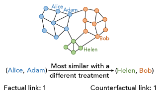
Unfortunately, the causal relationship between graph structure and link existence was largely ignored in previous work. Existing methods that learn from association are not able to capture essential factors to accurately predict missing links in test data. Take a specific social network as an example. Suppose Alice and Adam live in the same neighborhood and they are close friends. The association between neighborhood belonging and friendship could be too strong to discover the essential factors of friendship such as common interests or family relationships. Such factors could also be the cause of them living in the same neighborhood. So, our idea is to ask a counterfactual question: “would Alice and Adam still be close friends if they were not living in the same neighborhood?” If a graph learning model can learn the causal relationship by answering this counterfactual question, it will improve the accuracy of link prediction with such knowledge. Generally, the questions can be described as “would the link exist or not if the graph structure became different from observation?”

As known to many, counterfactual questions are the key component of causal inference and have been well defined in literature. A counterfactual question is usually framed with three factors: context (as a data point), manipulation (e.g., treatment, intervention, action, strategy), and outcome (Van der Laan & Petersen, 2007; Johansson et al., 2016). (To simplify the language, we use “treatment” to refer to the manipulation in this paper, as readers might be familiar more with the word “treatment.”) Given certain data context, it asks what the outcome would have been if the treatment had not been the observed value. In the scenario of link prediction, we consider the information of a pair of nodes as context, graph structural properties as treatment, and link existence as outcome. Recall the social network example. The context is the representations of Alice and Adam that are learned from their personal attributes and relationships with others on the social network. The treatment is whether live in the same neighborhood, which can be identified by community detection. And the outcome is their friendship.

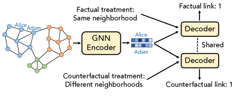
In this work, we propose a novel concept of “counterfactual link” that answers the counterfactual question and (based on this concept) a novel link prediction method (CFLP) that uses the counterfactual links as augmented data for graph representation learning. Figure 1 illustrates this two-step method. Suppose the treatment variable is defined as one type of global graph structure, e.g., the neighborhood assignment discovered by spectral clustering or community detection algorithms. We are wondering how likely the neighborhood distribution makes a difference on the link (non-)existence for each pair of nodes. So, given a pair of nodes (like Alice and Adam) and the treatment value on this pair (in the same neighborhood), we find a pair of nodes (like Helen and Bob) that satisfies two conditions: (1) it has a different treatment (in different neighborhoods) and (2) it is the most similar pair with the given pair of nodes. We name these matched pairs of nodes as counterfactual links. Note that the outcome of the counterfactual links can be either 1 or 0, depending on whether there exists an edge between the matched pair of nodes. The counterfactual link provides an unobservable outcome to the given pair of nodes under a counterfactual condition. The process of creating counterfactual links for all positive and negative training examples can be viewed as a graph data augmentation method, as it enriches the training set. Then, CFLP trains a link predictor (which is GNN-based) to learn the representation vectors of nodes to predict both the observed factual links and counterfactual links. In this Alice-Adam example, the link predictor is trained to estimate the individual treatment effect (ITE) of neighborhood assignment as $1-1=0$, where ITE is a metric for the effect of treatment on the outcome and zero indicates the given treatment has no effect on the outcome. So, the learner will try to discover the essential factors on the friendship between Alice and Adam. CFLP learns from the counterfactual links to find these factors for graph learning models to accurately predict missing links.

Contributions. Our main contributions can be summarized as follows. (1) This is the first work that aims at improving link prediction by causal inference, specifically, generating counterfactual links to answer counterfactual questions about link existence. (2) This work introduces CFLP that trains GNN-based link predictors to predict both factual and counterfactual links. It leverages causal relationship between global graph structure and link existence to enhance link prediction. (3) CFLP outperforms competitive baselines on several benchmark datasets. We analyze the impact of counterfactual links as well as the choice of treatment variable. This work sheds insights for improving graph machine learning with causal analysis, which has not been extensively studied yet, while the other direction (machine learning for causal inference) has been studied for long. Source code of the proposed CFLP method is publicly available at https://github.com/DM2-ND/CFLP.

2 Problem Definition

Notations

Let $G=(\mathcal{V},\mathcal{E})$ be an undirected graph of $N$ nodes, where $\mathcal{V}=\{v_{1},v_{2},\dots,v_{N}\}$ is the set of nodes and $\mathcal{E}\subseteq\mathcal{V}\times\mathcal{V}$ is the set of observed links. We denote the adjacency matrix as $\mathbf{A}\in\{0,1\}^{N\times N}$, where $A_{i,j}=1$ indicates nodes $v_{i}$ and $v_{j}$ are connected and vice versa. We denote the node feature matrix as $\mathbf{X}\in\mathbb{R}^{N\times F}$, where $F$ is the number of node features and $\mathbf{x}_{i}$ indicates the feature vector of node $v_{i}$ (the $i$-th row of $\mathbf{X}$).

In this work, we follow the commonly accepted problem definition of link prediction on graph data (Zhang & Chen, 2018; Zhang et al., 2020; Cai et al., 2021): Given an observed graph $G$ (with validation and testing links masked off), predict the link existence between every pair of nodes. More specifically, for the GNN-based link prediction methods, they learn low-dimensional node representations $\mathbf{Z}\in\mathbb{R}^{N\times H}$, where $H$ is the dimensional size of latent space such that $H\ll N$, and then use $\mathbf{Z}$ for the prediction of link existence between every node pair.

3 Proposed Method

3.1 Improving Graph Learning with Causal Model

(a) Causal modeling (not the target of our work but related to the idea we propose): Given $\mathbf{Z}$ and observed outcomes, find treatment effect of $T$ on $Y$.

(b) Graph learning with causal model (the proposed idea): leverage the estimated $\text{ITE}(A_{i,j}|T_{i,j})$ to improve the learning of $\mathbf{z}_{i}$ and $\mathbf{z}_{j}$.

Figure 2: Our proposed work improves graph representation learning by leveraging causal model.

Leveraging Causal Model(s)

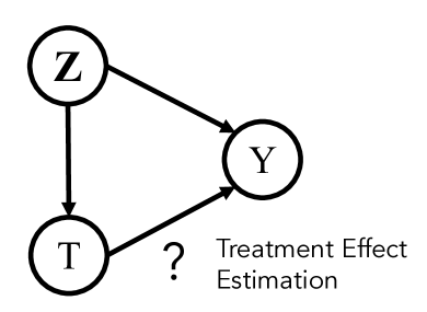
Counterfactual causal inference aims to find out the causal relationship between treatment and outcome by asking the counterfactual questions such as “would the outcome be different if the treatment was different?” (Morgan & Winship, 2015). Figure 2(a) is a typical example, in which we denote the context (confounder) as $\mathbf{Z}$, treatment as $T$, and the outcome as $Y$. Given the context, treatments, and their corresponding outcomes, counterfactual inference methods aim to find the effect of treatment on the outcome, which is usually measured by individual treatment effect (ITE) and its expectation averaged treatment effect (ATE) (Van der Laan & Petersen, 2007; Weiss et al., 2015). For a binary treatment variable $T=\{0,1\}$, denoting $g(\mathbf{z},T)$ as the outcome of $\mathbf{z}$ given the treatment $T$, we have $\text{ITE}(\mathbf{z})=g(\mathbf{z},1)-g(\mathbf{z},0)$, and $\text{ATE}=\mathbb{E}_{\mathbf{z}\sim\mathbf{Z}}~{}\text{ITE}(\mathbf{z})$.

Ideally, we need all potential outcomes of the contexts under all kinds of treatments to study the causal relationships (Morgan & Winship, 2015). However, in reality, the fact that we can only observe the outcome under one particular treatment prevents the ITE from being known (Johansson et al., 2016). Traditional causal inference methods use statistical learning approaches such as Neyman–Rubin causal model (BCM) and propensity score matching (PSM) to predict the value of ATE (Rubin, 1974, 2005).

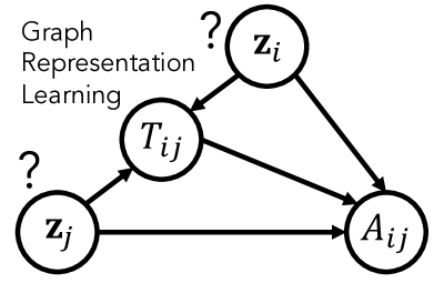
In this work, we look at link prediction with graph learning, which is to learn effective node representations $\mathbf{Z}$ for predicting link existence in test data. In Figure 2(b), $\mathbf{z}_{i}$ and $\mathbf{z}_{j}$ are representations of nodes $v_{i}$ and $v_{j}$, and the outcome $A_{i,j}$ is the link existence between $v_{i}$ and $v_{j}$. Here, the objective is different from classic causal inference. In graph learning, we want to improve the learning of $\mathbf{z}_{i}$ and $\mathbf{z}_{j}$ with the estimation on the effect of treatment $T_{i,j}$ on the outcome $A_{i,j}$. Specifically, for each pair of nodes $(v_{i},v_{j})$, its ITE can be estimated by

$$\text{ITE}_{(v_{i},v_{j})}=g((\mathbf{z}_{i},\mathbf{z}_{j}),1)-g((\mathbf{z}_{i},\mathbf{z}_{j}),0)\vspace{-0.03in}$$ (1)

and we use this information to improve the learning of $\mathbf{Z}$.

We denote by $\mathbf{A}$ the observed adjacency matrix as the factual outcomes, and denote by $\mathbf{A}^{CF}$ the unobserved matrix of the counterfactual links when the treatment is different as the counterfactual outcomes. We denote $\mathbf{T}\in\{0,1\}^{N\times N}$ as the binary factual treatment matrix, where $T_{i,j}$ indicates the treatment of the node pair $(v_{i},v_{j})$. We denote $\mathbf{T}^{CF}$ as the counterfactual treatment matrix where $T^{CF}_{i,j}=1-T_{i,j}$. We are interested in (a) estimating the counterfactual outcomes $\mathbf{A}^{CF}$ and (b) learning from both factual and counterfactual outcomes $\mathbf{A}$ and $\mathbf{A}^{CF}$ (as observed and augmented data) to enhance link prediction.

Treatment Variable

Previous works on GNN-based link prediction (Zhang & Chen, 2018; Zhang et al., 2020) have shown that the message passing-based GNNs are capable to capture the structural information (e.g., Katz index) for link prediction. Nevertheless, as illustrated by the Alice-Adam example in Section 1, the association between such structural information and actual link existence may be too strong for models to discover more essential factors than it, hence resulting in sub-optimal link prediction performance. Therefore, in this work, we use the global structural role of each node pair as its treatment. It’s worth mentioning that the causal model shown in Figure 2(b) does not limit the treatment to be structural roles, i.e., $T_{i,j}$ can be any binary property of node pair $(v_{i},v_{j})$. Without the loss of generality, we use Louvain (Blondel et al., 2008), an unsupervised approach that has been widely used for community detection, as an example. Louvain discovers community structure of a graph and assigns each node to one community. Then we can define the binary treatment variable as whether these two nodes in the pair belong to the same community. Let $c:\mathcal{V}\rightarrow\mathbb{N}$ be any graph mining/clustering method that outputs the index of community/cluster/neighborhood that each node belongs to. The treatment matrix $\mathbf{T}$ is defined as $T_{i,j}=1$ if $c(v_{i})=c(v_{j})$, and $T_{i,j}=0$ otherwise. For the choice of $c$, we suggest methods that group nodes based on global graph structural information, including but not limited to Louvain (Blondel et al., 2008), K-core (Bader & Hogue, 2003), and spectral clustering (Ng et al., 2001).

3.2 Counterfactual Links

To implement the solution based on above idea, we propose counterfactual links. As aforementioned, for each node pair, the observed data contains only the factual treatment and outcome, meaning that the link existence for the given node pair with an opposite treatment is unknown. Therefore, we use the outcome from the nearest observed context as a substitute. This type of matching on covariates is widely used to estimate treatment effects from observational data (Johansson et al., 2016; Alaa & Van Der Schaar, 2019). That is, we want to find the nearest neighbor with the opposite treatment for each observed node pairs and use the nearest neighbor’s outcome as a counterfactual link. Formally, $\forall(v_{i},v_{j})\in\mathcal{V}\times\mathcal{V}$, its counterfactual link $(v_{a},v_{b})$ is

$$(v_{a},v_{b})=\operatorname*{arg\,min}_{v_{a},v_{b}\in\mathcal{V}}\{h((v_{i},v_{j}),(v_{a},v_{b}))\text{ }|\text{ }T_{a,b}=1-T_{i,j}\},$$ (2)

where $h(\cdot,\cdot)$ is a metric of measuring the distance between a pair of node pairs (a pair of contexts). Nevertheless, finding the nearest neighbors by computing the distance between all pairs of node pairs is extremely inefficient and infeasible in application, which takes $O(N^{4})$ comparisons (as there are totally $O(N^{2})$ node pairs). Hence we implement Eq. 2 using node-level embeddings. Specifically, considering that we want to find the nearest node pair based on both the raw node features and structural features, we take the state-of-the-art unsupervised graph representation learning method MVGRL (Hassani & Khasahmadi, 2020) to learn the node embeddings $\tilde{\mathbf{X}}\in\mathbb{R}^{N\times\tilde{F}}$ from the observed graph (with validation and testing links masked off). We use $\tilde{\mathbf{X}}$ to find the nearest neighbors of node pairs. Therefore, $\forall(v_{i},v_{j})\in\mathcal{V}\times\mathcal{V}$, we define its counterfactual link $(v_{a},v_{b})$ as

$$(v_{a},v_{b})= \operatorname*{arg\,min}_{v_{a},v_{b}\in\mathcal{V}}\{d(\tilde{\mathbf{x}}_{i},\tilde{\mathbf{x}}_{a})+d(\tilde{\mathbf{x}}_{j},\tilde{\mathbf{x}}_{b})\text{ }|\text{ }$$ (3)

$$T_{a,b}=1-T_{i,j},d(\tilde{\mathbf{x}}_{i},\tilde{\mathbf{x}}_{a})+d(\tilde{\mathbf{x}}_{j},\tilde{\mathbf{x}}_{b})<2\gamma\},\vspace{-0.02in}$$

where $d(\cdot,\cdot)$ is specified as the Euclidean distance on the embedding space of $\tilde{\mathbf{X}}$, and $\gamma$ is a hyperparameter that defines the maximum distance that two nodes are considered as similar. When no node pair satisfies the above equation (i.e., there does not exist any node pair with opposite treatment that is close enough to the target node pair), we do not assign any nearest neighbor for the given node pair to ensure all the neighbors are similar enough (as substitutes) in the feature space. Thus, the counterfactual treatment matrix $\mathbf{T}^{CF}$ and the counterfactual adjacency matrix $\mathbf{A}^{CF}$ are defined as

$$T^{CF}_{i,j},A^{CF}_{i,j}=\begin{cases}1-T_{i,j},A_{a,b}&\text{, if }\exists$ $(v_{a},v_{b})\in\mathcal{V}\times\mathcal{V}\\ &\quad\text{ satisfies \lx@cref{creftype~refnum}{eq:nearest2};}\\ T_{i,j},A_{i,j}&\text{, otherwise}.\end{cases}$$ (4)

It is worth noting that the node embeddings $\tilde{\mathbf{X}}$ and the nearest neighbors are computed only once and do not change during the learning process. $\tilde{\mathbf{X}}$ is only used for finding the nearest neighbors.

Learning from Counterfactual Distributions

Let $P^{F}$ be the factual distribution of the observed contexts and treatments, and $P^{CF}$ be the counterfactual distribution that is composed of the observed contexts and opposite treatments. We define the empirical factual distribution $\hat{P}^{F}\sim P^{F}$ as $\hat{P}^{F}=\{(v_{i},v_{j},T_{i,j})\}^{N}_{i,j=1}$, and define the empirical counterfactual distribution $\hat{P}^{CF}\sim P^{CF}$ as $\hat{P}^{CF}=\{(v_{i},v_{j},T^{CF}_{i,j})\}^{N}_{i,j=1}$. Unlike traditional link prediction methods that take only $\hat{P}^{F}$ as input and use the observed outcomes $\mathbf{A}$ as the training target, we take advantage of the counterfactual distribution by using it as the augmented training data. That is, we use $\hat{P}^{CF}$ as a complementary input and use the counterfactual outcomes $\mathbf{A}^{CF}$ as the training target for the counterfactual data samples.

3.3 Learning from Counterfactual Links

In this subsection, we present the design of our model as well as the training method. The input of the model in CFLP includes (1) the observed graph data $\mathbf{A}$ and raw feature matrix $\mathbf{X}$, (2) the factual treatments $\mathbf{T}^{F}$ and counterfactual treatments $\mathbf{T}^{CF}$, and (3) the counterfactual links data $\mathbf{A}^{CF}$. The output contains link prediction logits in $\widehat{\mathbf{A}}$ and $\widehat{\mathbf{A}}^{CF}$ for the factual and counterfactual adjacency matrices $\mathbf{A}$ and $\mathbf{A}^{CF}$, respectively.

Graph Learning Model

The model consist of two trainable components: a graph encoder $f$ and a link decoder $g$. The graph encoder generates representation vectors of nodes from graph data. And the link decoder projects the representation vectors of node pairs into the link prediction logits. The choice of the graph encoder $f$ can be any end-to-end GNN model. Without the loss of generality, here we use the commonly used graph convolutional network (GCN) (Kipf & Welling, 2016a). Each layer of GCN is defined as

where $l$ is the layer index, $\tilde{\mathbf{A}}=\mathbf{A}+\mathbf{I}$ is the adjacency matrix with added self-loops, $\tilde{\mathbf{D}}$ is the diagonal degree matrix $\tilde{D}_{ii}=\sum_{j}\tilde{A}_{ij}$, $\mathbf{H}^{(0)}=\mathbf{X}$, $\mathbf{W}^{(l)}$ is the learnable weight matrix at the $l$-th layer, and $\sigma(\cdot)$ denotes the nonlinear activation ReLU. We denote $\mathbf{Z}=f(\mathbf{A},\mathbf{X})\in\mathbb{R}^{N\times H}$ as the output from the encoder’s last layer, i.e., the $H$-dimensional representation vectors of nodes. Following previous works (Zhang & Chen, 2018; Zhang et al., 2020), we compute the representation of a node pair as the Hadamard product of the vectors of the two nodes. That is, the representation for the node pair $(v_{i},v_{j})$ is $\mathbf{z}_{i}\odot\mathbf{z}_{j}\in\mathbb{R}^{H}$, where $\odot$ stands for the Hadamard product.

For the link decoder that predicts whether a link exists between a pair of nodes, we opt for simplicity and adopt a simple decoder based on multi-layer perceptron (MLP), given the representations of node pairs and their treatments. That is, the decoder $g$ is defined as

(6)

(7)

where $[\cdot,\cdot]$ stands for the concatenation of vectors, and $\widehat{\mathbf{A}}$ and $\widehat{\mathbf{A}}^{CF}$ can also be used for estimating the observed ITE as aforementioned in Eq. 1.

During the training process, data samples from the empirical factual distribution $\hat{P}^{F}$ and the empirical counterfactual distribution $\hat{P}^{CF}$ are fed into decoder $g$ and optimized towards $\mathbf{A}$ and $\mathbf{A}^{CF}$, respectively. That is, for the two distributions, the loss functions are as follows:

$$\mathcal{L}_{F}= \frac{1}{N^{2}}\sum_{i=1}^{N}\sum_{j=1}^{N}A_{i,j}\cdot\log\widehat{A}_{i,j}$$ (8)

$$+(1-A_{i,j})\cdot\log(1-\widehat{A}_{i,j}),$$

$$\mathcal{L}_{CF}= \frac{1}{N^{2}}\sum_{i=1}^{N}\sum_{j=1}^{N}A^{CF}_{i,j}\cdot\log\widehat{A}^{CF}_{i,j}$$ (9)

$$+(1-A^{CF}_{i,j})\cdot\log(1-\widehat{A}^{CF}_{i,j}).$$

Balancing Counterfactual Learning

In the training process, the above loss minimizations train the model on both the empirical factual distribution $\hat{P}^{F}\sim P^{F}$ and empirical counterfactual distribution $\hat{P}^{CF}\sim P^{CF}$ that are not necessarily equal – the training examples (node pairs) do not have to be aligned. However, at the stage of inference, the test data contains only observed (factual) samples. Such a gap between the training and testing data distributions exposes the model in the risk of covariant shift, which is a common issue in counterfactual representation learning (Johansson et al., 2016; Assaad et al., 2021).

To force the distributions of representations of factual distributions and counterfactual distributions to be similar, we adopt the discrepancy distance (Mansour et al., 2009; Johansson et al., 2016) as another training objective to regularize the representation learning. That is, we use the following loss term to minimize the distance between the learned representations from $\hat{P}^{F}$ and $\hat{P}^{CF}$:

$$\mathcal{L}_{disc}=\text{disc}(\hat{P}^{F}_{f},\hat{P}^{CF}_{f}),\text{ where }\text{disc}(P,Q)=||P-Q||_{F},$$ (10)

where $||\cdot||_{F}$ denotes the Frobenius Norm, and $\hat{P}^{F}_{f}$ and $\hat{P}^{CF}_{f}$ denote the node pair representations learned by graph encoder $f$ from factual distribution and counterfactual distribution, respectively. Specifically, the learned representations for $(v_{i},v_{j},T_{i,j})$ and $(v_{i},v_{j},T_{i,j}^{CF})$ are $[\mathbf{z}_{i}\odot\mathbf{z}_{j},T_{i,j}]$ (Eq. 6) and $[\mathbf{z}_{i}\odot\mathbf{z}_{j},T_{i,j}^{CF}]$ (Eq. 7), respectively.

Training

During the training of CFLP, we want the model to be optimized towards three targets: (1) accurate link prediction on the observed outcomes (Eq. 8), (2) accurate prediction on the counterfactual links (Eq. 9), and (3) regularization on the representation spaces learned from $\hat{P}^{F}$ and $\hat{P}^{CF}$ (Eq. 10). Therefore, the overall training loss of our proposed CFLP is

$$\mathcal{L}=\mathcal{L}_{F}+\alpha\cdot\mathcal{L}_{CF}+\beta\cdot\mathcal{L}_{disc},$$ (11)

where $\alpha$ and $\beta$ are hyperparameters to control the weights of counterfactual outcome estimation (link prediction) loss and discrepancy loss.

Algorithm 1 CFLP

  Input: $f$, $g$, $\mathbf{A}$, $\mathbf{X}$, $n\_epochs$, $n\_epoch\_ft$

  Compute $\mathbf{T}$ as presented in Section 3.1.

  Compute $\mathbf{T}^{CF},\mathbf{A}^{CF}$ by Eqs. 3 and 4.

  // model training

  for epoch in range($n\_epochs$) do

     $\mathbf{Z}=f(\mathbf{A},\mathbf{X})$.

     Get $\widehat{\mathbf{A}}$ and $\widehat{\mathbf{A}}^{CF}$ via $g$ with Eqs. 6 and 7.

     Update $\Theta_{f}$ and $\Theta_{g}$ with $\mathcal{L}$. (Eq. 11)

  end for

  // decoder fine-tuning

  Freeze $\Theta_{f}$ and re-initialize $\Theta_{g}$.

  $\mathbf{Z}=f(\mathbf{A},\mathbf{X})$.

  for epoch in range($n\_epochs\_ft$) do

     Get $\widehat{\mathbf{A}}$ via $g$ with Eq. 6.

     Update $\Theta_{g}$ with $\mathcal{L}_{F}$. (Eq. 8)

  end for

  // inference

  $\mathbf{Z}=f(\mathbf{A},\mathbf{X})$.

  Get $\widehat{\mathbf{A}}$ and $\widehat{\mathbf{A}}^{CF}$ via $g$ with Eqs. 6 and 7.

  Output: $\widehat{\mathbf{A}}$ for link prediction, $\widehat{\mathbf{A}}^{CF}$.

Summary

Algorithm 1 summarizes the whole process of CFLP. The first step is to compute the factual and counterfactual treatments $\mathbf{T}$, $\mathbf{T}^{CF}$ as well as the counterfactual links $\mathbf{A}^{CF}$. Then, the second step trains the graph learning model on both the observed factual link existence and generated counterfactual link existence with the integrated loss function (Eq. 11). Note that the discrepancy loss (Eq. 10) is computed on the representations of node pairs learned by the graph encoder $f$, so the decoder $g$ is trained with data from both $\hat{P}^{F}$ and $\hat{P}^{CF}$ without balancing the constraints. Therefore, after the model is sufficiently trained, we freeze the graph encoder $f$ and fine-tune $g$ with only the factual data. Finally, after the decoder is sufficiently fine-tuned, we output the link prediction logits for both the factual and counterfactual adjacency matrices.

Table 1: Statistics of datasets used in the experiments.

Dataset	Cora	CiteSeer	PubMed	Facebook	OGB-ddi
# nodes	2,708	3,327	19,717	4,039	4,267
# links	5,278	4,552	44,324	88,234	1,334,889
# validation node pairs	1,054	910	8,864	17,646	235,371
# test node pairs	2,110	1,820	17,728	35,292	229,088

Complexity

The complexity of the first step (finding counterfactual links with nearest neighbors) is proportional to the number of node pairs. When $\gamma$ is set as a small value to obtain indeed similar node pairs, this step (Eq. 3) uses constant time. Moreover, the computation in Eq. 3 can be parallelized. Therefore, the time complexity is $O(N^{2}/C)$ where $C$ is the number of processes. For the complexity of the second step (training counterfactual learning model), the GNN encoder has time complexity of $O(LH^{2}N+LH|\mathcal{E}|)$ (Wu et al., 2020), where $L$ is the number of GNN layers and $H$ is the size of node representations. Given that we sample the same number of non-existing links as that of observed links during training, the complexity of a three-layer MLP decoder is $O(((H+1)\cdot d_{h}+d_{h}\cdot 1)|\mathcal{E}|)=O(d_{h}(H+2)|\mathcal{E}|)$, where $d_{h}$ is the number of neurons in the hidden layer. Therefore, the second step has linear time complexity w.r.t. the sum of node and edge counts.

Limitations

First, as mentioned above, the computation of finding counterfactual links has a worst-case complexity of $O(N^{2})$. Second, CFLP performs counterfactual prediction with only a single treatment; however, there are quite a few kinds of graph structural information that can be considered as treatments. Future work can leverage the rich structural information by bundled treatments (Zou et al., 2020) in the generation of counterfactual links.

4 Experiments

Table 2: Link prediction performances measured by Hits@20. Best performance and best baseline performance are marked with bold and underline, respectively.

	Cora	CiteSeer	PubMed	Facebook	OGB-ddi
Node2Vec	49.96$\pm$2.51	47.78$\pm$1.72	39.19$\pm$1.02	24.24$\pm$3.02	23.26$\pm$2.09
MVGRL	19.53$\pm$2.64	14.07$\pm$0.79	14.19$\pm$0.85	14.43$\pm$0.33	10.02$\pm$1.01
VGAE	45.91$\pm$3.38	44.04$\pm$4.86	23.73$\pm$1.61	37.01$\pm$0.63	11.71$\pm$1.96
SEAL	51.35$\pm$2.26	40.90$\pm$3.68	28.45$\pm$3.81	40.89$\pm$5.70	30.56$\pm$3.86
LGLP	62.98$\pm$0.56	57.43$\pm$3.71	–	37.86$\pm$2.13	–
GCN	49.06$\pm$1.72	55.56$\pm$1.32	21.84$\pm$3.87	53.89$\pm$2.14	37.07$\pm$5.07
GSAGE	53.54$\pm$2.96	53.67$\pm$2.94	39.13$\pm$4.41	45.51$\pm$3.22	53.90$\pm$4.74
JKNet	48.21$\pm$3.86	55.60$\pm$2.17	25.64$\pm$4.11	52.25$\pm$1.48	60.56$\pm$8.69
Our proposed CFLP with different graph encoders
CFLP w/ GCN	60.34$\pm$2.33	59.45$\pm$2.30	34.12$\pm$2.72	53.95$\pm$2.29	52.51$\pm$1.09
CFLP w/ GSAGE	57.33$\pm$1.73	53.05$\pm$2.07	43.07$\pm$2.36	47.28$\pm$3.00	75.49$\pm$4.33
CFLP w/ JKNet	65.57$\pm$1.05	68.09$\pm$1.49	44.90$\pm$2.00	55.22$\pm$1.29	86.08$\pm$1.98

Table 3: Link prediction performances measured by AUC. Best performance and best baseline performance are marked with bold and underline, respectively.

	Cora	CiteSeer	PubMed	Facebook	OGB-ddi
Node2Vec	84.49$\pm$0.49	80.00$\pm$0.68	80.32$\pm$0.29	86.49$\pm$4.32	90.83$\pm$0.02
MVGRL	75.07$\pm$3.63	61.20$\pm$0.55	80.78$\pm$1.28	79.83$\pm$0.30	81.45$\pm$0.99
VGAE	88.68$\pm$0.40	85.35$\pm$0.60	95.80$\pm$0.13	98.66$\pm$0.04	93.08$\pm$0.15
SEAL	92.55$\pm$0.50	85.82$\pm$0.44	96.36$\pm$0.28	99.60$\pm$0.02	97.85$\pm$0.17
LGLP	91.30$\pm$0.05	89.41$\pm$0.13	–	98.51$\pm$0.01	–
GCN	90.25$\pm$0.53	71.47$\pm$1.40	96.33$\pm$0.80	99.43$\pm$0.02	99.82$\pm$0.05
GSAGE	90.24$\pm$0.34	87.38$\pm$1.39	96.78$\pm$0.11	99.29$\pm$0.04	99.93$\pm$0.02
JKNet	89.05$\pm$0.67	88.58$\pm$1.78	96.58$\pm$0.23	99.43$\pm$0.02	99.94$\pm$0.01
Our proposed CFLP with different graph encoders
CFLP w/ GCN	92.55$\pm$0.50	89.65$\pm$0.20	96.99$\pm$0.08	99.38$\pm$0.01	99.44$\pm$0.05
CFLP w/ GSAGE	92.61$\pm$0.52	91.84$\pm$0.20	97.01$\pm$0.01	99.34$\pm$0.10	99.83$\pm$0.05
CFLP w/ JKNet	93.05$\pm$0.24	92.12$\pm$0.47	97.53$\pm$0.17	99.31$\pm$0.04	99.94$\pm$0.01

4.1 Experimental Setup

We conduct experiments on five benchmark datasets including citation networks (Cora, CiteSeer, PubMed (Yang et al., 2016)), social network (Facebook (McAuley & Leskovec, 2012)), and drug-drug interaction network (OGB-ddi (Wishart et al., 2018)) from the Open Graph Benchmark (OGB) (Hu et al., 2020). For the first four datasets, we randomly select 10%/20% of the links and the same numbers of disconnected node pairs as validation/test samples. The links in the validation and test sets are masked off from the training graph. For OGB-ddi, we used the OGB official train/validation/test splits. Statistics for the datasets are shown in Table 1, with more details in Appendix. We use K-core (Bader & Hogue, 2003) clusters as the default treatment variable. We evaluate CFLP on three commonly used GNN encoders: GCN (Kipf & Welling, 2016a), GSAGE (Hamilton et al., 2017), and JKNet (Xu et al., 2018). We compare the link prediction performance of CFLP against Node2Vec (Grover & Leskovec, 2016), MVGRL (Hassani & Khasahmadi, 2020), VGAE (Kipf & Welling, 2016b), SEAL (Zhang & Chen, 2018), LGLP (Cai et al., 2021), and GNNs with MLP decoder. We report averaged test performance and their standard deviation over 20 runs with different random parameter initializations. Other than the most commonly used of Area Under ROC Curve (AUC), we report Hits@20 (one of the primary metrics on OGB leaderboard) as a more challenging metric, as it expects models to rank positive edges higher than nearly all negative edges.

Besides performance comparison on link prediction, we will answer two questions to suggest a way of choosing a treatment variable for creating counterfactual links: (Q1) Does CFLP sufficiently learn the observed averaged treatment effect (ATE) derived from the counterfactual links? (Q2) What is the relationship between the estimated ATE learned in the method and the prediction performance? If the answer to Q1 is yes, then the answer to Q2 will indicate how to choose treatment based on observed ATE. To answer the Q1, we calculate the observed ATE ($\widehat{\text{ATE}}_{obs}$) by comparing the observed links in $\mathbf{A}$ and created counterfactual links $\mathbf{A}^{CF}$ that have opposite treatments. And we calculate the estimated ATE ($\widehat{\text{ATE}}_{est}$) by comparing the predicted links in $\widehat{\mathbf{A}}$ and predicted counterfactual links $\widehat{\mathbf{A}}^{CF}$. Formally, $\widehat{\text{ATE}}_{obs}$ and $\widehat{\text{ATE}}_{est}$ are defined as

$$\widehat{\text{ATE}}_{obs}= \frac{1}{N^{2}}\sum_{i=1}^{N}\sum_{j=1}^{N}{\{}\mathbf{T}\odot(\mathbf{A}-\mathbf{A}^{CF})$$ (12)

$$+(\mathbf{1}_{N\times N}-\mathbf{T})\odot(\mathbf{A}^{CF}-\mathbf{A}){\}}_{i,j}.$$

$$\widehat{\text{ATE}}_{est}= \frac{1}{N^{2}}\sum_{i=1}^{N}\sum_{j=1}^{N}{\{}\mathbf{T}\odot(\widehat{\mathbf{A}}-\widehat{\mathbf{A}}^{CF})$$ (13)

$$+(\mathbf{1}_{N\times N}-\mathbf{T})\odot(\widehat{\mathbf{A}}^{CF}-\widehat{\mathbf{A}}){\}}_{i,j}.$$

The treatment variables we will investigate are generally graph clustering or community detection methods, such as K-core (Bader & Hogue, 2003), stochastic block model (SBM) (Karrer & Newman, 2011), spectral clustering (SpecC) (Ng et al., 2001), propagation clustering (PropC) (Raghavan et al., 2007), Louvain (Blondel et al., 2008), common neighbors (CommN), Katz index, and hierarchical clustering (Ward) (Ward Jr, 1963). We use JKNet (Xu et al., 2018) as default graph encoder.

Implementation details and supplementary experimental results (e.g., sensitivity on $\gamma$, ablation study on $\mathcal{L}_{CF}$ and $\mathcal{L}_{disc}$) can be found in Appendix. Source code is available in supplementary material.

4.2 Experimental Results

Link Prediction

Tables 2 and 3 show the link prediction performance of Hits@20 and AUC by all methods. LGLP on PubMed and OGB-ddi are missing due to the out of memory error when running the official code package from the authors. We observe that our CFLP on different graph encoders achieve similar or better performances compared with baselines. The only exception is the AUC on Facebook where most methods have close-to-perfect AUC. As AUC is a relatively easier metric comparing with Hits@20, most methods achieved good performance on AUC. We observe that CFLP with JKNet almost consistently achieves the best performance and outperforms baselines significantly on Hits@20. Specifically, comparing with the best baseline, CFLP improves relatively by 16.4% and 0.8% on Hits@20 and AUC, respectively. Comparing with the best performing baselines, which are also GNN-based, CFLP benefits from learning with both observed link existence ($\mathbf{A}$) and our defined counterfactual links ($\mathbf{A}^{CF}$).

ATE with Different Treatments

Tables 4 and 5 show the link prediction performance, $\widehat{\text{ATE}}_{obs}$, and $\widehat{\text{ATE}}_{est}$ of CFLP (with JKNet) when using different treatments. The treatments in Tables 4 and 5 are sorted by the Hits@20 performance. Bigger ATE indicates stronger causal relationship between the treatment and outcome, and vice versa. We observe: (1) the rankings of $\widehat{\text{ATE}}_{est}$ and $\widehat{\text{ATE}}_{obs}$ are positively correlated with Kendell’s ranking coefficient (Abdi, 2007) of 0.67 and 0.57 for Cora and CiteSeer, respectively. Hence, CFLP was sufficiently trained to learn the causal relationship between graph structure information and link existence; (2) $\widehat{\text{ATE}}_{obs}$ and $\widehat{\text{ATE}}_{est}$ are both negatively correlated with the link prediction performance, showing that we can pick a proper treatment prior to training a model with CFLP. Using the treatment that has the weakest causal relationship with link existence is likely to train the model to capture more essential factors on the outcome, in a way similar to denoising the unrelated information from the representations. While methods that learn from only observed data may assume strongly positive correlation for this treatment, the counterfactual data are more useful to complement the partial observations for learning better representations.

Table 4: Results of CFLP with different treatments on Cora. (sorted by Hits@20)

	Hits@20	$\widehat{\text{ATE}}_{obs}$	$\widehat{\text{ATE}}_{est}$
K-core	65.6$\pm$1.1	0.002	0.013$\pm$0.003
SBM	64.2$\pm$1.1	0.006	0.023$\pm$0.015
CommN	62.3$\pm$1.6	0.007	0.053$\pm$0.021
PropC	61.7$\pm$1.4	0.037	0.059$\pm$0.065
Ward	61.2$\pm$2.3	0.001	0.033$\pm$0.012
SpecC	59.3$\pm$2.8	0.002	0.033$\pm$0.011
Louvain	57.6$\pm$1.8	0.025	0.138$\pm$0.091
Katz	56.6$\pm$3.4	0.740	0.802$\pm$0.041

Table 5: Results of CFLP with different treatments on CiteSeer. (sorted by Hits@20)

	Hits@20	$\widehat{\text{ATE}}_{obs}$	$\widehat{\text{ATE}}_{est}$
SBM	71.6 $\pm$1.9	0.004	0.005 $\pm$0.001
K-core	68.1$\pm$1.5	0.002	0.010$\pm$0.002
Ward	67.0$\pm$1.7	0.003	0.037$\pm$0.009
PropC	64.6$\pm$3.6	0.141	0.232$\pm$0.113
Louvain	63.3$\pm$2.5	0.126	0.151$\pm$0.078
SpecC	59.9$\pm$1.3	0.009	0.166$\pm$0.034
Katz	57.3$\pm$0.5	0.245	0.224$\pm$0.037
CommN	56.8$\pm$4.9	0.678	0.195$\pm$0.034

5 Related Work

Link Prediction

With its wide applications, link prediction has drawn attention from many research communities including statistical machine learning and data mining. Stochastic generative methods based on stochastic block models (SBM) are developed to generate links (Mehta et al., 2019). In data mining, matrix factorization (Menon & Elkan, 2011), heuristic methods (Philip et al., 2010; Martínez et al., 2016), and graph embedding methods (Cui et al., 2018) have been applied to predict links in the graph. Heuristic methods compute the similarity score of nodes based on their neighborhoods. These methods can be generally categorized into first-order, second-order, and high-order heuristics based on the maximum distance of the neighbors. Graph embedding methods learn latent node features via embedding lookup and use them for link prediction (Perozzi et al., 2014; Tang et al., 2015; Grover & Leskovec, 2016; Wang et al., 2016).

In the past few years, GNNs have shown promising results on various graph-based tasks with their ability of learning from features and custom aggregations on structures (Kipf & Welling, 2016a; Hamilton et al., 2017; Ma et al., 2021; Jiang et al., 2022). With node pair representations and an attached MLP or inner-product decoder, GNNs can be used for link prediction (Davidson et al., 2018; Yang et al., 2018; Zhang et al., 2020; Yun et al., 2021; Zhu et al., 2021b; Wang et al., 2021a, b). For example, VGAE used GCN to learn node representations and reconstruct the graph structure (Kipf & Welling, 2016b). SEAL extracted a local subgraph around each target node pair and then learned local subgraph representation for link prediction (Zhang & Chen, 2018). Following the scheme of SEAL, Cai & Ji (2020) proposed to improve local subgraph representation learning by multi-scale graph representation. And LGLP proposed to invert the local subgraphs to line graphs (Cai et al., 2021). However, little work has studied to use causal inference for improving link prediction.

Causal Inference

Causal inference methods usually re-weighted samples based on propensity score (Rosenbaum & Rubin, 1983; Austin, 2011) to remove confounding bias from binary treatments. Recently, several works studied about learning treatment invariant representation to predict the counterfactual outcomes (Shalit et al., 2017; Li & Fu, 2017; Yao et al., 2018; Yoon et al., 2018; Hassanpour & Greiner, 2019a, b; Bica et al., 2020). Few recent works combined causal inference with graph learning (Sherman & Shpitser, 2020; Bevilacqua et al., 2021; Lin et al., 2021; Feng et al., 2021). For example, Sherman & Shpitser (2020) proposed network intervention to study the effect of link creation on network structure changes.

As a mean of learning the causality between treatment and outcome, counterfactual prediction has been used for a variety of applications such as recommender systems (Wang et al., 2020b; Xu et al., 2020), health care (Alaa & van der Schaar, 2017; Pawlowski et al., 2020), and decision making (Kusner et al., 2017; Pitis et al., 2020). To infer the causal relationships, previous work usually estimated the ITE via function fitting models (Kuang et al., 2017; Wager & Athey, 2018; Kuang et al., 2019; Assaad et al., 2021).

Graph Data Augmentation

Graph data augmentation (GDA) methods generate perturbed or modified graph data (Zhao et al., 2021a, b) to improve the generalizability of graph machine learning models. Two comprehensive surveys of graph data augmentation are given by Zhao et al. (2022) and Ding et al. (2022). So far, most GDA methods have been focusing on node-level tasks (Park et al., 2021) and graph-level tasks (Liu et al., 2022; Luo et al., 2022). Due to the non-Euclidean structure of graphs, most GDA work focused on modifying the graph structure. E.g., edge dropping methods (Rong et al., 2019; Zheng et al., 2020; Luo et al., 2021) drop edges during training to reduce overfitting. Zhao et al. (2021a) used link predictor to manipulate the graph structure and improve the graph’s homophily. Recently, several works also combined GDA with self-supervised learning objectives such as contrastive learning (You et al., 2020, 2021; Zhu et al., 2021a) and consistency loss (Wang et al., 2020a; Feng et al., 2020). Nevertheless, GDA for link prediction has been under-explored.

6 Conclusion and Future Work

In this work, we presented the novel concept of counterfactual link and a novel graph learning method for link prediction (CFLP). The counterfactual links answered the counterfactual questions on the link existence and were used as augmented training data, with which CFLP accurately predicted missing links by exploring the causal relationship between global graph structure and link existence. Extensive experiments demonstrated that CFLP achieved the state-of-the-art performance on benchmark datasets. This work sheds insights that a good use of causal models (even basic ones) can greatly improve the performance of (graph) machine learning tasks such as link prediction. We note that the use of more sophistically designed causal models may lead to larger improvements for machine learning tasks, which can be a valuable future direction for the research community. Other than cluster-based global graph structure as treatment, other choices (with both empirical and theoretical analyses) are also worthy of exploration.

Appendix A Additional Dataset Details

In this section, we provide some additional dataset details. All the datasets used in this work are publicly available.

Citation Networks

Cora, CiteSeer, and PubMed are citation networks that were first used by Yang et al. (2016) and then commonly used as benchmarks in GNN-related literature (Kipf & Welling, 2016a; Veličković et al., 2017). In these citation networks, the nodes are published papers and features are bag-of-word vectors extracted from the corresponding paper. Links represent the citation relation between papers. We loaded the datasets with the DGL package.

Social Network

The Facebook dataset is a social network constructed from friends lists from Facebook (McAuley & Leskovec, 2012). The nodes are Facebook users and links indicate the friendship relation on Facebook. The node features were constructed from the user profiles and anonymized by McAuley & Leskovec (2012).

Drug-Drug Interaction Network

The OGB-ddi dataset was constructed from a public Drug database (Wishart et al., 2018) and provided by the Open Graph Benchmark (OGB) (Hu et al., 2020). Each node in this graph represents an FDA-approved or experimental drug and edges represent the existence of unexpected effect when the two drugs are taken together. This dataset does not contain any node features, and it can be downloaded with the dataloader provided by OGB.

Appendix B Details on Implementation and Hyperparameters

All the experiments in this work were conducted on a Linux server with Intel Xeon Gold 6130 Processor (16 Cores @2.1Ghz), 96 GB of RAM, and 4 RTX 2080Ti cards (11 GB of RAM each). Our method are implemented with Python 3.8.5 with PyTorch. Source code is publicly available at https://github.com/DM2-ND/CFLP.

Baseline Methods

For baseline methods, we use official code packages from the authors for MVGRL (Hassani & Khasahmadi, 2020), SEAL (Zhang & Chen, 2018), and LGLP (Cai et al., 2021). We use a public implementation for VGAE (Kipf & Welling, 2016b) and OGB implementations for Node2Vec and baseline GNNs. For fair comparison, we set the size of node/link representations to be 256 of all methods.

CFLP

We use the Adam optimizer with a simple cyclical learning rate scheduler (Smith, 2017), in which the learning rate waves cyclically between the given learning rate ($lr$) and 1e-4 in every 70 epochs (50 warmup steps and 20 annealing steps). We implement the GNN encoders with torch_geometric (Fey & Lenssen, 2019). Same with the baselines, we set the size of all hidden layers and node/link representations of CFLP as 256. The graph encoders all have three layers and JKNet has mean pooling for the final aggregation layer. The decoder is a 3-layer MLP with a hidden layer of size 64 and ELU as the nonlinearity. As the Euclidean distance used in Eq. 3 has a range of $[0,\infty)$, the value of $\gamma$ depends on the distribution of all-pair node embedding distances, which varies for different datasets. Therefore, we set the value of $\gamma$ as the $\gamma_{pct}$-percentile of all-pair node embedding distances. Commands for reproducing the experiments are included in README.md.

Hyperparameter Searching Space

We manually tune the following hyperparameters over range: $lr\in\{0.005,0.01,0.05,0.1,0.2\}$, $\alpha\in\{0.001,0.01,0.1,1,2\}$, $\beta\in\{0.001,0.01,0.1,1,2\}$, $\gamma_{pct}\in\{10,20,30\}$.

Treatments

For the graph clustering or community detection methods we used as treatments, we use the implementation from scikit-network for Louvain (Blondel et al., 2008), SpecC (Ng et al., 2001), PropC (Raghavan et al., 2007), and Ward (Ward Jr, 1963). We used implementation of K-core (Bader & Hogue, 2003) from networkx. We used SBM (Karrer & Newman, 2011) from a public implementation by Funke & Becker (2019). For CommN and Katz, we set $T_{i,j}=1$ if the number of common neighbors or Katz index between $v_{i}$ and $v_{j}$ are greater or equal to 2 or 2 times the average of all Katz index values, respectively. For SpecC, we set the number of clusters as 16. For SBM, we set the number of communities as 16. These settings are fixed for all datasets.

Table 6: Link prediction performances measured by Hits@50. Best performance and best baseline performance are marked with bold and underline, respectively.

	Cora	CiteSeer	PubMed	Facebook	OGB-ddi
Node2Vec	63.64$\pm$0.76	54.57$\pm$1.40	50.73$\pm$1.10	43.91$\pm$1.03	24.34$\pm$1.67
MVGRL	29.97$\pm$3.06	26.48$\pm$0.98	16.96$\pm$0.56	17.06$\pm$0.19	12.03$\pm$0.11
VGAE	60.36$\pm$2.71	54.68$\pm$3.15	41.98$\pm$0.31	51.36$\pm$0.93	23.00$\pm$1.66
SEAL	51.68$\pm$2.85	54.55$\pm$1.77	42.85$\pm$2.03	57.20$\pm$1.85	40.85$\pm$2.97
LGLP	71.43$\pm$0.75	69.98$\pm$0.16	–	56.22$\pm$0.49	–
GCN	64.93$\pm$1.62	63.38$\pm$1.73	39.20$\pm$6.47	69.90$\pm$0.65	73.70$\pm$3.99
GSAGE	63.18$\pm$3.39	61.71$\pm$2.43	54.81$\pm$2.67	62.53$\pm$4.24	86.83$\pm$3.85
JKNet	62.64$\pm$1.40	62.26$\pm$2.10	45.16$\pm$3.18	68.81$\pm$1.76	91.48$\pm$2.41
Our proposed CFLP with different graph encoders
CFLP w/ GCN	72.61$\pm$0.92	69.85$\pm$1.11	55.00$\pm$1.95	70.47$\pm$0.77	62.47$\pm$1.53
CFLP w/ GSAGE	73.25$\pm$0.94	64.75$\pm$2.27	58.16$\pm$1.40	63.89$\pm$2.08	83.32$\pm$3.61
CFLP w/ JKNet	75.49$\pm$1.54	77.01$\pm$1.92	62.80$\pm$0.79	71.41$\pm$0.61	93.07$\pm$1.14

Table 7: Link prediction performances measured by Average Precision (AP). Best performance and best baseline performance are marked with bold and underline, respectively.

	Cora	CiteSeer	PubMed	Facebook	OGB-ddi
Node2Vec	88.53$\pm$0.42	84.42$\pm$0.48	87.15$\pm$0.12	99.07$\pm$0.02	98.39$\pm$0.04
MVGRL	76.47$\pm$3.07	67.40$\pm$0.52	82.00$\pm$0.97	82.37$\pm$0.35	81.12$\pm$1.77
VGAE	89.89$\pm$0.50	86.97$\pm$0.78	95.97$\pm$0.16	98.60$\pm$0.04	95.28$\pm$0.11
SEAL	89.08$\pm$0.57	88.55$\pm$0.32	96.33$\pm$0.28	99.51$\pm$0.03	98.39$\pm$0.21
LGLP	93.05$\pm$0.03	91.62$\pm$0.09	–	98.62$\pm$0.01	–
GCN	91.42$\pm$0.45	90.87$\pm$0.52	96.19$\pm$0.88	99.42$\pm$0.02	99.86$\pm$0.03
GSAGE	91.52$\pm$0.46	89.43$\pm$1.15	96.93$\pm$0.11	99.27$\pm$0.06	99.93$\pm$0.01
JKNet	90.50$\pm$0.22	90.42$\pm$1.34	96.56$\pm$0.31	99.41$\pm$0.02	99.95$\pm$0.01
Our proposed CFLP with different graph encoders
CFLP w/ GCN	93.77$\pm$0.49	91.84$\pm$0.20	97.16$\pm$0.08	99.40$\pm$0.01	99.60$\pm$0.03
CFLP w/ GSAGE	93.55$\pm$0.49	90.80$\pm$0.87	97.10$\pm$0.08	99.29$\pm$0.06	99.88$\pm$0.04
CFLP w/ JKNet	94.24$\pm$0.28	93.92$\pm$0.41	97.69$\pm$0.13	99.35$\pm$0.02	99.96$\pm$0.01

Table 8: Link prediction performance of CFLP (w/ JKNet) on Cora and CiteSeer when removing $\mathcal{L}_{CF}$ or $\mathcal{L}_{disc}$ or both versus normal setting.

	Cora		CiteSeer
	Hits@20	AUC	Hits@20	AUC
CFLP ($\alpha=0$)	58.58$\pm$0.23	89.16$\pm$0.93	65.49$\pm$2.18	91.01$\pm$0.64
CFLP ($\beta=0$)	62.27$\pm$0.84	92.96$\pm$0.34	66.92$\pm$1.84	91.98$\pm$0.17
CFLP ($\alpha=\beta=0$)	58.52$\pm$0.83	88.79$\pm$0.28	64.69$\pm$3.25	90.61$\pm$0.64
CFLP	65.57$\pm$1.05	93.05$\pm$0.24	68.09$\pm$1.49	92.12$\pm$0.47

Table 9: Link prediction performance of CFLP (w/ JKNet) on Cora and CiteSeer with node embeddings ($\tilde{\mathbf{X}}$) learned from different methods.

	Cora		CiteSeer		OGB-ddi
	Hits@20	AUC	Hits@20	AUC	Hits@20	AUC
(MVGRL)	65.57$\pm$1.05	93.05$\pm$0.24	68.09$\pm$1.49	92.12$\pm$0.47	86.08$\pm$1.98	99.94$\pm$0.01
(GRACE)	62.54$\pm$1.41	92.28$\pm$0.69	68.68$\pm$1.75	93.80$\pm$0.36	82.30$\pm$3.32	99.93$\pm$0.01
(DGI)	61.04$\pm$1.52	92.99$\pm$0.49	72.17$\pm$1.08	93.34$\pm$0.51	85.61$\pm$1.66	99.94$\pm$0.01

Appendix C Additional Experimental Results and Discussions

Link Prediction

Tables 6 and 7 show the link prediction performance of Hits@50 and Average Precision (AP) by all methods. LGLP on PubMed and OGB-ddi are missing due to the out of memory error when running the code package from the authors. Similar to the results in Tables 2 and 3, we observe that our CFLP on different graph encoders achieve similar or better performances compared with baselines, with the only exception of AP on Facebook where most methods have close-to-perfect AP. From Tables 2, 3, 6 and 7, we observe that CFLP achieves improvement over all GNN architectures (averaged across datasets). Specifically, CFLP improves 25.6% (GCN), 12.0% (GSAGE), and 36.3% (JKNet) on Hits@20, 9.6% (GCN), 5.0% (GSAGE), and 17.8% (JKNet) on Hits@50, 5.6% (GCN), 1.6% (GSAGE), and 1.9% (JKNet) on AUC, and 0.8% (GCN), 0.8% (GSAGE), and 1.8% (JKNet) on AP. We note that CFLP with JKNet almost consistently achieves the best performance and outperforms baselines significantly on Hits@50. Specifically, compared with the best baseline, CFLP improves relatively by 6.8% and 0.9% on Hits@50 and AP, respectively.

Ablation Study on Losses

For the ablative studies of $\mathcal{L}_{CF}$ (Eq. 9) and $\mathcal{L}_{disc}$ (Eq. 10), we show their effect by removing them from the integrated loss function (Eq. 11). Table 8 shows the results of CFLP on Cora and CiteSeer under different settings ($\alpha=0$, $\beta=0$, $\alpha=\beta=0$, and original setting). We observe that CFLP in the original setting achieves the best performance. The performance drops significantly when having $\alpha=0$, i.e., not using any counterfactual data during training. We note that having $\beta=0$, i.e., not using the discrepancy loss, also lowers the performance. Therefore, both $\mathcal{L}_{CF}$ and $\mathcal{L}_{disc}$ are essential for improving the link prediction performance.

Ablation Study on Node Embedding $\tilde{\mathbf{X}}$

As the node embedding $\tilde{\mathbf{X}}$ is used in the early step of CFLP for finding the counterfactual links, the quality of $\tilde{\mathbf{X}}$ may affect the later learning process. Therefore, we also evaluate CFLP with different state-of-the-art unsupervised graph representation learning methods: MVGRL (Hassani & Khasahmadi, 2020), DGI (Velickovic et al., 2019), and GRACE (Zhu et al., 2020). Table 9 shows the link prediction performance of CFLP (w/ JKNet) on Cora and CiteSeer with different node embeddings. We observe that the choice of the method for learning $\tilde{\mathbf{X}}$ does have an impact on the later learning process as well as the link prediction performance. Nevertheless, Table 9 shows CFLP’s advantage can be consistently observed with different choices of methods for learning $\tilde{\mathbf{X}}$, as CFLP with $\tilde{\mathbf{X}}$ learned from all three methods showed promising link prediction performance.

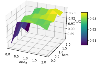
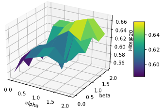
Sensitivity Analysis of $\alpha$ and $\beta$

Figure 3 shows the AUC performance of CFLP on Cora with different combinations of $\alpha$ and $\beta$. We observe that the performance is the poorest when $\alpha=\beta=0$ and gradually improves and gets stable as $\alpha$ and $\beta$ increase, showing that CFLP is generally robust to the hyperparameters $\alpha$ and $\beta$, and the optimal values are easy to locate.

(a) AUC performance.

(b) Hits@20 performance.

Figure 3: Performance of CFLP on Cora w.r.t different combinations of $\alpha$ and $\beta$.

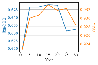
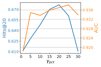
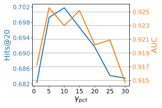
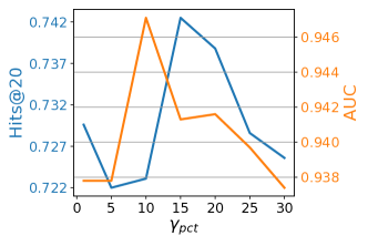
Sensitivity Analysis of $\gamma$

Figure 4 shows the Hits@20 and AUC performance on link prediction of CFLP (with JKNet) on Cora and CiteSeer with different treatments and $\gamma_{pct}$. We observe that the performance is generally good when $10\leq\gamma_{pct}\leq 20$ and gradually get worse when the value of $\gamma_{pct}$ is too small or too large, showing that CFLP is robust to $\gamma$ and the optimal $\gamma$ is easy to find.

(a) Performances of CFLP on Cora when using K-core as treatment.

(b) Performances of CFLP on Cora when using SBM as treatment.

(c) Performances of CFLP on CiteSeer when using K-core as treatment.

(d) Performances of CFLP on CiteSeer when using SBM as treatment.

Figure 4: Hits@20 and AUC performances of CFLP (w/ JKNet) on Cora and CiteSeer with different treatments w.r.t. different $\gamma_{pct}$ value.

References

- Abdi (2007) Abdi, H. The kendall rank correlation coefficient. Encyclopedia of Measurement and Statistics. Sage, Thousand Oaks, CA, pp. 508–510, 2007.
- Alaa & Van Der Schaar (2019) Alaa, A. and Van Der Schaar, M. Validating causal inference models via influence functions. In International Conference on Machine Learning, pp. 191–201, 2019.
- Alaa & van der Schaar (2017) Alaa, A. M. and van der Schaar, M. Bayesian inference of individualized treatment effects using multi-task gaussian processes. Advances in Neural Information Processing Systems, 2017.
- Assaad et al. (2021) Assaad, S., Zeng, S., Tao, C., Datta, S., Mehta, N., Henao, R., Li, F., and Duke, L. C. Counterfactual representation learning with balancing weights. In International Conference on Artificial Intelligence and Statistics, pp. 1972–1980. PMLR, 2021.
- Austin (2011) Austin, P. C. An introduction to propensity score methods for reducing the effects of confounding in observational studies. Multivariate behavioral research, 46(3):399–424, 2011.
- Bader & Hogue (2003) Bader, G. D. and Hogue, C. W. An automated method for finding molecular complexes in large protein interaction networks. BMC bioinformatics, 4(1):1–27, 2003.
- Bennett et al. (2007) Bennett, J., Lanning, S., et al. The netflix prize. In Proceedings of KDD cup and workshop, volume 2007, pp. 35. Citeseer, 2007.
- Bevilacqua et al. (2021) Bevilacqua, B., Zhou, Y., and Ribeiro, B. Size-invariant graph representations for graph classification extrapolations. arXiv preprint arXiv:2103.05045, 2021.
- Bica et al. (2020) Bica, I., Alaa, A. M., Jordon, J., and van der Schaar, M. Estimating counterfactual treatment outcomes over time through adversarially balanced representations. arXiv preprint arXiv:2002.04083, 2020.
- Blondel et al. (2008) Blondel, V. D., Guillaume, J.-L., Lambiotte, R., and Lefebvre, E. Fast unfolding of communities in large networks. Journal of statistical mechanics: theory and experiment, 2008(10):P10008, 2008.
- Cai & Ji (2020) Cai, L. and Ji, S. A multi-scale approach for graph link prediction. In Proceedings of the AAAI Conference on Artificial Intelligence, volume 34, pp. 3308–3315, 2020.
- Cai et al. (2021) Cai, L., Li, J., Wang, J., and Ji, S. Line graph neural networks for link prediction. IEEE Transactions on Pattern Analysis and Machine Intelligence, 2021.
- Cui et al. (2018) Cui, P., Wang, X., Pei, J., and Zhu, W. A survey on network embedding. IEEE Transactions on Knowledge and Data Engineering, 31(5):833–852, 2018.
- Davidson et al. (2018) Davidson, T. R., Falorsi, L., De Cao, N., Kipf, T., and Tomczak, J. M. Hyperspherical variational auto-encoders. arXiv preprint arXiv:1804.00891, 2018.
- Ding et al. (2022) Ding, K., Xu, Z., Tong, H., and Liu, H. Data augmentation for deep graph learning: A survey. arXiv preprint arXiv:2202.08235, 2022.
- Feng et al. (2021) Feng, F., Huang, W., He, X., Xin, X., Wang, Q., and Chua, T.-S. Should graph convolution trust neighbors? a simple causal inference method. In Proceedings of the 44th International ACM SIGIR Conference on Research and Development in Information Retrieval, pp. 1208–1218, 2021.
- Feng et al. (2020) Feng, W., Zhang, J., Dong, Y., Han, Y., Luan, H., Xu, Q., Yang, Q., Kharlamov, E., and Tang, J. Graph random neural network for semi-supervised learning on graphs. arXiv preprint arXiv:2005.11079, 2020.
- Fey & Lenssen (2019) Fey, M. and Lenssen, J. E. Fast graph representation learning with pytorch geometric. arXiv preprint arXiv:1903.02428, 2019.
- Funke & Becker (2019) Funke, T. and Becker, T. Stochastic block models: A comparison of variants and inference methods. PloS one, 14(4), 2019.
- Grover & Leskovec (2016) Grover, A. and Leskovec, J. node2vec: Scalable feature learning for networks. In Proceedings of the 22nd ACM SIGKDD international conference on Knowledge discovery and data mining, pp. 855–864, 2016.
- Hamilton et al. (2017) Hamilton, W. L., Ying, R., and Leskovec, J. Inductive representation learning on large graphs. arXiv preprint arXiv:1706.02216, 2017.
- Hassani & Khasahmadi (2020) Hassani, K. and Khasahmadi, A. H. Contrastive multi-view representation learning on graphs. In International Conference on Machine Learning, pp. 4116–4126. PMLR, 2020.
- Hassanpour & Greiner (2019a) Hassanpour, N. and Greiner, R. Counterfactual regression with importance sampling weights. In IJCAI, pp. 5880–5887, 2019a.
- Hassanpour & Greiner (2019b) Hassanpour, N. and Greiner, R. Learning disentangled representations for counterfactual regression. In International Conference on Learning Representations, 2019b.
- Hu et al. (2020) Hu, W., Fey, M., Zitnik, M., Dong, Y., Ren, H., Liu, B., Catasta, M., and Leskovec, J. Open graph benchmark: Datasets for machine learning on graphs. arXiv preprint arXiv:2005.00687, 2020.
- Jiang et al. (2022) Jiang, M., Jung, T., Karl, R., and Zhao, T. Federated dynamic graph neural networks with secure aggregation for video-based distributed surveillance. ACM Transactions on Intelligent Systems and Technology (TIST), 13(4):1–23, 2022.
- Johansson et al. (2016) Johansson, F., Shalit, U., and Sontag, D. Learning representations for counterfactual inference. In International conference on machine learning, pp. 3020–3029, 2016.
- Karrer & Newman (2011) Karrer, B. and Newman, M. E. Stochastic blockmodels and community structure in networks. Physical review E, 83(1):016107, 2011.
- Kazemi & Poole (2018) Kazemi, S. M. and Poole, D. Simple embedding for link prediction in knowledge graphs. In Advances in Neural Information Processing Systems, volume 31, 2018.
- Kipf & Welling (2016a) Kipf, T. N. and Welling, M. Semi-supervised classification with graph convolutional networks. arXiv preprint arXiv:1609.02907, 2016a.
- Kipf & Welling (2016b) Kipf, T. N. and Welling, M. Variational graph auto-encoders. arXiv preprint arXiv:1611.07308, 2016b.
- Kuang et al. (2017) Kuang, K., Cui, P., Li, B., Jiang, M., Yang, S., and Wang, F. Treatment effect estimation with data-driven variable decomposition. In Proceedings of the AAAI Conference on Artificial Intelligence, volume 31, 2017.
- Kuang et al. (2019) Kuang, K., Cui, P., Li, B., Jiang, M., Wang, Y., Wu, F., and Yang, S. Treatment effect estimation via differentiated confounder balancing and regression. ACM Transactions on Knowledge Discovery from Data (TKDD), 14(1):1–25, 2019.
- Kusner et al. (2017) Kusner, M. J., Loftus, J. R., Russell, C., and Silva, R. Counterfactual fairness. Advances in Neural Information Processing Systems, 2017.
- Li & Fu (2017) Li, S. and Fu, Y. Matching on balanced nonlinear representations for treatment effects estimation. In Advances in Neural Information Processing Systems, 2017.
- Lin et al. (2021) Lin, W., Lan, H., and Li, B. Generative causal explanations for graph neural networks. In International Conference on Machine Learning, 2021.
- Liu et al. (2022) Liu, G., Zhao, T., Xu, J., Luo, T., and Jiang, M. Graph rationalization with environment-based augmentations. In Proceedings of the 28th ACM SIGKDD International Conference on Knowledge Discovery & Data Mining, 2022.
- Luo et al. (2021) Luo, D., Cheng, W., Yu, W., Zong, B., Ni, J., Chen, H., and Zhang, X. Learning to drop: Robust graph neural network via topological denoising. In Proceedings of the 14th ACM International Conference on Web Search and Data Mining, pp. 779–787, 2021.
- Luo et al. (2022) Luo, Y., McThrow, M., Au, W. Y., Komikado, T., Uchino, K., Maruhash, K., and Ji, S. Automated data augmentations for graph classification. arXiv preprint arXiv:2202.13248, 2022.
- Ma et al. (2021) Ma, Y., Liu, X., Zhao, T., Liu, Y., Tang, J., and Shah, N. A unified view on graph neural networks as graph signal denoising. In Proceedings of the 30th ACM International Conference on Information & Knowledge Management, pp. 1202–1211, 2021.
- Mansour et al. (2009) Mansour, Y., Mohri, M., and Rostamizadeh, A. Domain adaptation: Learning bounds and algorithms. arXiv preprint arXiv:0902.3430, 2009.
- Martínez et al. (2016) Martínez, V., Berzal, F., and Cubero, J.-C. A survey of link prediction in complex networks. ACM computing surveys (CSUR), 49(4):1–33, 2016.
- McAuley & Leskovec (2012) McAuley, J. J. and Leskovec, J. Learning to discover social circles in ego networks. In Advances in Neural Information Processing Systems, volume 2012, pp. 548–56, 2012.
- Mehta et al. (2019) Mehta, N., Duke, L. C., and Rai, P. Stochastic blockmodels meet graph neural networks. In International Conference on Machine Learning, pp. 4466–4474, 2019.
- Menon & Elkan (2011) Menon, A. K. and Elkan, C. Link prediction via matrix factorization. In Joint european conference on machine learning and knowledge discovery in databases, pp. 437–452. Springer, 2011.
- Morgan & Winship (2015) Morgan, S. L. and Winship, C. Counterfactuals and causal inference. Cambridge University Press, 2015.
- Ng et al. (2001) Ng, A., Jordan, M., and Weiss, Y. On spectral clustering: Analysis and an algorithm. Advances in neural information processing systems, 14:849–856, 2001.
- Park et al. (2021) Park, H., Lee, S., Kim, S., Park, J., Jeong, J., Kim, K.-M., Ha, J.-W., and Kim, H. J. Metropolis-hastings data augmentation for graph neural networks. Advances in Neural Information Processing Systems, 34, 2021.
- Pawlowski et al. (2020) Pawlowski, N., Castro, D. C., and Glocker, B. Deep structural causal models for tractable counterfactual inference. Advances in Neural Information Processing Systems, 2020.
- Perozzi et al. (2014) Perozzi, B., Al-Rfou, R., and Skiena, S. Deepwalk: Online learning of social representations. In Proceedings of the 20th ACM SIGKDD international conference on Knowledge discovery and data mining, pp. 701–710, 2014.
- Philip et al. (2010) Philip, S. Y., Han, J., and Faloutsos, C. Link mining: Models, algorithms, and applications. Springer, 2010.
- Pitis et al. (2020) Pitis, S., Creager, E., and Garg, A. Counterfactual data augmentation using locally factored dynamics. Advances in Neural Information Processing Systems, 2020.
- Raghavan et al. (2007) Raghavan, U. N., Albert, R., and Kumara, S. Near linear time algorithm to detect community structures in large-scale networks. Physical review E, 76(3):036106, 2007.
- Rong et al. (2019) Rong, Y., Huang, W., Xu, T., and Huang, J. Dropedge: Towards deep graph convolutional networks on node classification. In International Conference on Learning Representations, 2019.
- Rosenbaum & Rubin (1983) Rosenbaum, P. R. and Rubin, D. B. The central role of the propensity score in observational studies for causal effects. Biometrika, 70(1):41–55, 1983.
- Rubin (1974) Rubin, D. B. Estimating causal effects of treatments in randomized and nonrandomized studies. Journal of educational Psychology, 66(5):688, 1974.
- Rubin (2005) Rubin, D. B. Causal inference using potential outcomes: Design, modeling, decisions. Journal of the American Statistical Association, 100(469):322–331, 2005.
- Shalit et al. (2017) Shalit, U., Johansson, F. D., and Sontag, D. Estimating individual treatment effect: generalization bounds and algorithms. In International Conference on Machine Learning, pp. 3076–3085, 2017.
- Sherman & Shpitser (2020) Sherman, E. and Shpitser, I. Intervening on network ties. In Uncertainty in Artificial Intelligence, pp. 975–984. PMLR, 2020.
- Smith (2017) Smith, L. N. Cyclical learning rates for training neural networks. In 2017 IEEE winter conference on applications of computer vision (WACV), pp. 464–472. IEEE, 2017.
- Stanfield et al. (2017) Stanfield, Z., Coşkun, M., and Koyutürk, M. Drug response prediction as a link prediction problem. Scientific reports, 7(1):1–13, 2017.
- Tang et al. (2015) Tang, J., Qu, M., Wang, M., Zhang, M., Yan, J., and Mei, Q. Line: Large-scale information network embedding. In Proceedings of the 24th international conference on world wide web, pp. 1067–1077, 2015.
- Van der Laan & Petersen (2007) Van der Laan, M. J. and Petersen, M. L. Causal effect models for realistic individualized treatment and intention to treat rules. The international journal of biostatistics, 3(1), 2007.
- Veličković et al. (2017) Veličković, P., Cucurull, G., Casanova, A., Romero, A., Lio, P., and Bengio, Y. Graph attention networks. arXiv preprint arXiv:1710.10903, 2017.
- Velickovic et al. (2019) Velickovic, P., Fedus, W., Hamilton, W. L., Liò, P., Bengio, Y., and Hjelm, R. D. Deep graph infomax. In ICLR (Poster), 2019.
- Wager & Athey (2018) Wager, S. and Athey, S. Estimation and inference of heterogeneous treatment effects using random forests. Journal of the American Statistical Association, 113(523):1228–1242, 2018.
- Wang et al. (2016) Wang, D., Cui, P., and Zhu, W. Structural deep network embedding. In Proceedings of the 22nd ACM SIGKDD international conference on Knowledge discovery and data mining, pp. 1225–1234, 2016.
- Wang et al. (2021a) Wang, D., Zhang, Z., Ma, Y., Zhao, T., Jiang, T., Chawla, N., and Jiang, M. Modeling co-evolution of attributed and structural information in graph sequence. IEEE Transactions on Knowledge and Data Engineering, 2021a.
- Wang et al. (2021b) Wang, D., Zhao, T., Chawla, N. V., and Jiang, M. Dynamic attributed graph prediction with conditional normalizing flows. In 2021 IEEE International Conference on Data Mining (ICDM), pp. 1385–1390. IEEE, 2021b.
- Wang et al. (2020a) Wang, Y., Wang, W., Liang, Y., Cai, Y., Liu, J., and Hooi, B. Nodeaug: Semi-supervised node classification with data augmentation. In Proceedings of the 26th ACM SIGKDD International Conference on Knowledge Discovery & Data Mining, pp. 207–217, 2020a.
- Wang et al. (2020b) Wang, Z., Chen, X., Wen, R., Huang, S.-L., Kuruoglu, E. E., and Zheng, Y. Information theoretic counterfactual learning from missing-not-at-random feedback. Advances in Neural Information Processing Systems, 2020b.
- Ward Jr (1963) Ward Jr, J. H. Hierarchical grouping to optimize an objective function. Journal of the American statistical association, 58(301):236–244, 1963.
- Weiss et al. (2015) Weiss, J., Kuusisto, F., Boyd, K., Liu, J., and Page, D. Machine learning for treatment assignment: Improving individualized risk attribution. In AMIA Annual Symposium Proceedings, volume 2015, pp. 1306. American Medical Informatics Association, 2015.
- Wishart et al. (2018) Wishart, D. S., Feunang, Y. D., Guo, A. C., Lo, E. J., Marcu, A., Grant, J. R., Sajed, T., Johnson, D., Li, C., Sayeeda, Z., et al. Drugbank 5.0: a major update to the drugbank database for 2018. Nucleic acids research, 46(D1):D1074–D1082, 2018.
- Wu et al. (2020) Wu, Z., Pan, S., Chen, F., Long, G., Zhang, C., and Philip, S. Y. A comprehensive survey on graph neural networks. IEEE transactions on neural networks and learning systems, 2020.
- Xu et al. (2020) Xu, D., Ruan, C., Korpeoglu, E., Kumar, S., and Achan, K. Adversarial counterfactual learning and evaluation for recommender system. Advances in Neural Information Processing Systems, 2020.
- Xu et al. (2018) Xu, K., Li, C., Tian, Y., Sonobe, T., Kawarabayashi, K.-i., and Jegelka, S. Representation learning on graphs with jumping knowledge networks. In International Conference on Machine Learning, pp. 5453–5462, 2018.
- Yang et al. (2018) Yang, H., Pan, S., Zhang, P., Chen, L., Lian, D., and Zhang, C. Binarized attributed network embedding. In 2018 IEEE International Conference on Data Mining (ICDM), pp. 1476–1481. IEEE, 2018.
- Yang et al. (2016) Yang, Z., Cohen, W., and Salakhudinov, R. Revisiting semi-supervised learning with graph embeddings. In International conference on machine learning, pp. 40–48, 2016.
- Yao et al. (2018) Yao, L., Li, S., Li, Y., Huai, M., Gao, J., and Zhang, A. Representation learning for treatment effect estimation from observational data. Advances in Neural Information Processing Systems, 31, 2018.
- Yoon et al. (2018) Yoon, J., Jordon, J., and Van Der Schaar, M. Ganite: Estimation of individualized treatment effects using generative adversarial nets. In International Conference on Learning Representations, 2018.
- You et al. (2020) You, Y., Chen, T., Sui, Y., Chen, T., Wang, Z., and Shen, Y. Graph contrastive learning with augmentations. Advances in Neural Information Processing Systems, 33:5812–5823, 2020.
- You et al. (2021) You, Y., Chen, T., Shen, Y., and Wang, Z. Graph contrastive learning automated. arXiv preprint arXiv:2106.07594, 2021.
- Yun et al. (2021) Yun, S., Kim, S., Lee, J., Kang, J., and Kim, H. J. Neo-gnns: Neighborhood overlap-aware graph neural networks for link prediction. Advances in Neural Information Processing Systems, 34, 2021.
- Zhang & Chen (2018) Zhang, M. and Chen, Y. Link prediction based on graph neural networks. In Advances in Neural Information Processing Systems, 2018.
- Zhang et al. (2020) Zhang, M., Li, P., Xia, Y., Wang, K., and Jin, L. Revisiting graph neural networks for link prediction. arXiv preprint arXiv:2010.16103, 2020.
- Zhao et al. (2021a) Zhao, T., Liu, Y., Neves, L., Woodford, O., Jiang, M., and Shah, N. Data augmentation for graph neural networks. In Proceedings of the AAAI Conference on Artificial Intelligence, volume 35, pp. 11015–11023, 2021a.
- Zhao et al. (2021b) Zhao, T., Ni, B., Yu, W., Guo, Z., Shah, N., and Jiang, M. Action sequence augmentation for early graph-based anomaly detection. In Proceedings of the 30th ACM International Conference on Information & Knowledge Management, pp. 2668–2678, 2021b.
- Zhao et al. (2022) Zhao, T., Liu, G., Günnemann, S., and Jiang, M. Graph data augmentation for graph machine learning: A survey. arXiv preprint arXiv:2202.08871, 2022.
- Zheng et al. (2020) Zheng, C., Zong, B., Cheng, W., Song, D., Ni, J., Yu, W., Chen, H., and Wang, W. Robust graph representation learning via neural sparsification. In International Conference on Machine Learning, pp. 11458–11468, 2020.
- Zhu et al. (2020) Zhu, Y., Xu, Y., Yu, F., Liu, Q., Wu, S., and Wang, L. Deep graph contrastive representation learning. arXiv preprint arXiv:2006.04131, 2020.
- Zhu et al. (2021a) Zhu, Y., Xu, Y., Yu, F., Liu, Q., Wu, S., and Wang, L. Graph contrastive learning with adaptive augmentation. In Proceedings of the Web Conference 2021, pp. 2069–2080, 2021a.
- Zhu et al. (2021b) Zhu, Z., Zhang, Z., Xhonneux, L.-P., and Tang, J. Neural bellman-ford networks: A general graph neural network framework for link prediction. arXiv preprint arXiv:2106.06935, 2021b.
- Zou et al. (2020) Zou, H., Cui, P., Li, B., Shen, Z., Ma, J., Yang, H., and He, Y. Counterfactual prediction for bundle treatment. Advances in Neural Information Processing Systems, 33, 2020.