Incremental formation of scale-free fitness networks

Fabio Vanni111Correspondent author: fabio.vanni@sciencespo.fr Sciences Po, OFCE , France Center for Nonlinear Sciences, University of North Texas, USA
Abstract

In the paper, we present an incremental approach in the construction of scale free networks with hidden variables. The work arises from the necessity to generate that type of networks with a given number of links instead of obtaining a random configurations for a given set of parameters as in the usual literature. I propose an analytical approach of network evolution models gathering information along time based on the construction of a stochastic process on the space of possible networks. The analytical solution is eact in a case of multigraph network, meanwhile in simple graph we deal with important finite size effects. We show the statistical properties of this network such as number of isolated nodes, degree correlations and multilinks, also discussing the limitations of such predictions in real networks. Numerical simulations are used tu support the analytical calculations. On the computational side, such evolutive network construction allows to regulate the connectivity of the network obtaining desired values of connectivity density used as control parameter of the system. As a consequence, an incremental generetive approach is more suitable in those situation we want to control the number of links in the system while the number of nodes are kept fixed.


JEL codes: D85, C63, G21

Keywords: Network formation, incremental generative evolution, stochastic process.

1 Introduction

Network theory provides a natural way to model interconnections and its application to banking and finance has brought to a growing body of academic research on financial networks, bloomed over the past few years. The network approach to risk and stability has challenged the standard wisdom that a higher degree of interconnectedness is always desirable to achieve financial stability. A large part of network theory to financial markets has been focused on the analysis on how unexpected exogenous shocks propagate through a complex financial network where shocks can force a financial units to default. Diverse authors have developed a contagion and systemic risk models with both random ans scale-free structure networks as by Gai and Kapadia, [18] and [23]. In the following paper we describe a class of network models with attachment rules governed by intrinsic node fitness. This fitness is a measure of attractiveness and also a measure of a node’s robustness against failure. In the network representation agents are the nodes of the graph while the edges encode interactions. In the field of networks formation literature Dorogovtsev and Mendes, [15], there are random generated models where the set of nodes are fixed and dynamic networks growth models where or number of nodes and/or edges changes over time. In the present work we deal with a random generated model for scale-free networks where, contrary to the standard approach Caldarelli and Chessa, [11], it is possible to control the total number of edges (equivalently the average degree) at the end of procedure. To some extent, our prescription is the equivalent of Erdos-Renyi random graph generation as opposite to the Gilbert prescription. Despite the fact that the two prescriptions bring to the same degree distribution in limit of infinite number of nodes. Hidden variable models are models that avoid the need of assumptions of perfect knowledge about network topology (as preferential attachment). The linking rules for edges in such models are governed by some measure of the intrinsic quality of the node. In fact, hidden variable models are purely driven by static node intrinsic fitness and the topology of the network is determined by an attachment kernel function that describes the probability that a node with a certain fitness originates a link towards a node with another fitness, and the probability density that describes the distribution of fitness in the system. On the other side, degree dependent growth models new nodes have information about the connectivity of the entire network (Barabasi’s preferential attachment). For fitness driven networks it is sufficient to assume that nodes have information about the ranking of some derived topological independent quantity. For example, the balance sheet structure of a firm or a bank is more likely to be accessible to an investor than the absolute number of other investors invested in a particular company. The association of attractiveness and robustness to a failure is of great interest to organizations that can influence the underlying free parameters, e.g. distribution of fitness, as well as the average node-degree in the system as in in the interbank lending market, where the linking function is given fixed and cannot be influenced, but policy maker or regulator can reshape the fitness distribution by the introduction of a tax.

A graph process, denoted by G𝐺G is a method of constructing a network by adding a link to a graph G0subscript𝐺0G_{0} by choosing one with equal likelihood out of all possible links. Gtsubscript𝐺𝑑G_{t} is the network constructed after t𝑑t of these steps. The characterization of complex networks can be addressed by considering them as either static or dynamic entities. The most frequent static perspective is grounded on constructing a probability space (i.e., a probability measure on the space of possible networks); this probability model allows for a compact network characterization. Network evolution models gather information along time and they are grounded on the construction of a stochastic process on the space of possible networks. In particular, the fitness network model can be achieved following two approaches:

  1. 1.

    Random Generation G​(N,p)𝐺𝑁𝑝G(N,p): is a probability space on the setof graphs with N𝑁N nodes where each link in the graph is added independently with probability p𝑝p. The number of links L𝐿L is a random variable. We calculate once the matrix of making a link per each node and then assign randomly 111’s and 00’s to the adjacency matrix of the network.

  2. 2.

    Incremental Generation G​(N,L)𝐺𝑁𝐿G(N,L): is a probability space of all unlabeled graphs with N𝑁N nodes and L𝐿L links. We start with N𝑁N isolated nodes and connect two nodes per time step. The number of links L𝐿L is chosen to be fixed and deterministic. In this case we can control the average degree ⟨k⟩delimited-βŸ¨βŸ©π‘˜\langle k\rangle adding L𝐿L links to the network one by one.

In both versions, fitness models are characterized by an attachment kernel and a fitness distribution ρ​(x)𝜌π‘₯\rho(x). The attachment kernel f​(x,y)𝑓π‘₯𝑦f(x,y) describes the probability that a node with fitness xπ‘₯x originates a new edge toward a node with fitness y𝑦y. The fitness of each node is static over the lifetime of the network and is drawn from the probability density ρ​(x)𝜌π‘₯\rho(x). The classical random approach to the study of hidden variable graph rests on the work of Caldarelli etΒ al., [10], Servedio etΒ al., [28] who find directly the degree distribution and some statistical properties. A generalization of such models has been deeply addressed by BogunΓ‘ and Pastor-Satorras, [3], Serrano etΒ al., 2007a [26] which makes uses of a microscopic description of the system. Finally a more recent approach instead, look at such network from a evolutionary perspective, where links are sequentially deployed at each time step Bedogne and Rodgers, [2], Hoppe and Rodgers, [19]. The paper contributes to give an analytical description of a incremental formation of hidden variable networks with factorizable linking probability. We provide a master equation for the evolution of the degree probability distribution, and the evolution of expected number of isolated nodes. Further we will discuss some properties of the networks such as its degree distribution shape over time and its finite size effects as well as correlations among nodes in the case both of simple graph and multi-link version of the model. At the end, in the paper, we compare the previous analytical estimations to the Montecarlo simulations of the model to test the reliability of the theoretical description so giving the possibility to discuss some important implications on the use of a incremental formulation of hidden variable networks.

2 Incremental Model

Among all the possible real applications, in financial situations it is reasonable to think that two nodes will be connected depending on some of their intrinsic properties such as social status or information content. In this way, two nodes become connected when the link creates a mutual benefit Caldarelli, [9]. Therefore we build a financial network model in which each node i𝑖i (i=1,…,N)𝑖1…𝑁(i=1,...,N) is assigned a ” fitness ” described by a random real variable xisubscriptπ‘₯𝑖x_{i} distributed according to a certain probability distribution ρ​(x)𝜌π‘₯\rho(x). Each pair of nodes (i,j)𝑖𝑗(i,j) is then connected with a probability depending on the fitnesses or types of the two nodes, pi,j=f​(xi,xj)subscript𝑝𝑖𝑗𝑓subscriptπ‘₯𝑖subscriptπ‘₯𝑗p_{i,j}=f(x_{i},x_{j}), where f𝑓f is a given function222In the case where f=c​o​n​s​t.π‘“π‘π‘œπ‘›π‘ π‘‘f=const., the present model is equivalent to an Erdos-Renyi graph (random graph).. In this model the probability to have a link between two nodes depend on the fitness of the two nodes via a bi-dimensional linking function. There are different particular choices of such function, as expressed in Caldarelli, [9] and Montagna and Lux, [23]. The one we use in the present paper is a factorizable form of the type:

f​(x,y)=g​(x)​h​(y),𝑓π‘₯𝑦𝑔π‘₯β„Žπ‘¦f(x,y)=g(x)h(y), (1)

where in principle xπ‘₯x and y𝑦y can be two different peculiarities of the node, for example, in stock network, one peculiarity of the node can be the portfolio volume and the other the asset information. In the case of bank financial market such function provides the probability that a bank i𝑖i lends money to bank j𝑗j, and such banks (nodes) have only one peculiarity that is their financial size (assets for example) xisubscriptπ‘₯𝑖x_{i} and xjsubscriptπ‘₯𝑗x_{j}333Note that using the terminology of DEBIT/CREDIT the linking probability are reversed in terms of out-degree and in-degree, because the links are reversed in directions: who lands is creditor, who borrows is debtor. Now the links goes from debtors to creditors because debtors should give back the money they borrowed. so f​(xi,xj)=f~​(xj,xi)𝑓subscriptπ‘₯𝑖subscriptπ‘₯𝑗~𝑓subscriptπ‘₯𝑗subscriptπ‘₯𝑖f(x_{i},x_{j})=\tilde{f}(x_{j},x_{i}), where f~~𝑓\tilde{f} is the linking function for debit/credit connection so in the following formulas we nedd to exchange the term i​n𝑖𝑛in to o​u​tπ‘œπ‘’π‘‘out if we speaks in terms of credits and debits for all network properties. In other terms the Adjacency matrix in trasposed (or just exchange the exponents α𝛼\alpha and β𝛽\beta). Such peculiarites can be consider as random variable drawn from a density function. Combination of different fitness distributions and linking functions can bring to different structures and behaviors of networks. The empirical observations int he field of interbank markets suggest an appropriate linking function that reproduce the fact that small banks usually lend money to the biggest banks of the system, which in turn redistribute liquidity to the external financial markets or within the interbank market itself. As regard with the fitness ρ​(x)𝜌π‘₯\rho(x), one can choose any kind of distribution, however we select a Pareto distribution, particularly in its truncated version as widely discussed in the next sections. At this point we introduce the temporal prescription to generate a network that describes a generalization of the hidden variable models for a incremental point of view. Anyway we will still recover the particular situation in asymptotic regime. This kind of procedure has also another technical application (as in Bottazzi etΒ al., [8]), it allows to generate a given type of scale-free fitness network with a given connectivity (or average degree for finite networks). The network building algorithm is derived with the following steps:

  • β€’

    Start with N𝑁N nodes. Links are deployed one by one, not all at the same time.

  • β€’

    A link is added to a pair of nodes (i,j)𝑖𝑗(i,j) with probability, f​(xi,xj)/βˆ‘k,lf​(xk,xl)𝑓subscriptπ‘₯𝑖subscriptπ‘₯𝑗subscriptπ‘˜π‘™π‘“subscriptπ‘₯π‘˜subscriptπ‘₯𝑙f(x_{i},x_{j})/\sum_{k,l}f(x_{k},x_{l}). from j𝑗j to i𝑖i in a directed outgoing direction.

  • β€’

    The processes of adding nodes continues until a given number of links L𝐿L have been added.

In the present model the number of nodes remains constant during the network’s evolution, while the number of links increases linearly with time. As a result the average degree also increases linearly with time:

⟨k​(t)⟩∼tN=LNsimilar-todelimited-βŸ¨βŸ©π‘˜π‘‘π‘‘π‘πΏπ‘\langle{k}(t)\rangle\sim\frac{t}{N}=\frac{L}{N} (2)

In the simple graph formation, at each time step, each new link connects previously unconnected nodes, so that the number of links coincides with time passed from th origin.. After a sufficient number of links have been created the graph go towards the all to all condition for Lβ†’N​(Nβˆ’1)/2→𝐿𝑁𝑁12L\to N(N-1)/2 so that the network becomes a complete graph in which all nodes have degree km​a​x=Nβˆ’1subscriptπ‘˜π‘šπ‘Žπ‘₯𝑁1k_{max}=N-1 and even if the time passes no new link can be created, so the correspondence between number of links and time breaks. Although the network is static i.e. it contains a fixed number of nodes, the process in which edges are added can be understood as a dynamic procedure. Links are deployed one by one, not all at the same time snapshot. The probability that a node with fitness xπ‘₯x increases its out-degree by one during the step of the addition of a link is defined:

ν​(x)=βˆ‘lNf​(x,xl)βˆ‘i=1Nβˆ‘j=1Nf​(xi,xj),𝜈π‘₯superscriptsubscript𝑙𝑁𝑓π‘₯subscriptπ‘₯𝑙superscriptsubscript𝑖1𝑁superscriptsubscript𝑗1𝑁𝑓subscriptπ‘₯𝑖subscriptπ‘₯𝑗\displaystyle\nu(x)=\frac{\sum_{l}^{N}f(x,x_{l})}{\sum_{i=1}^{N}\sum_{j=1}^{N}f(x_{i},x_{j})}, (3)

that is the probability that a link is formed originating from a node with fitness xπ‘₯x. The normalization factor takes in account all the possible links that could be selected. For large number of nodes N𝑁N , fitness can be considered as a continuous variable, so we replace the sum used for discrete random variables with an integral over the set of possible values that is the average number of nodes with fitness xπ‘₯x as N​(x)=ρ​(x)​N𝑁π‘₯𝜌π‘₯𝑁N(x)=\rho(x)N. So the discrete eq.(3) becomes:

ν​(x)=Nβ€‹βˆ«0∞f​(x,y)​ρ​(y)​𝑑yN2β€‹βˆ«0∞∫0∞f​(x,y)​ρ​(x)​ρ​(y)​𝑑x​𝑑y.𝜈π‘₯𝑁superscriptsubscript0𝑓π‘₯π‘¦πœŒπ‘¦differential-d𝑦superscript𝑁2superscriptsubscript0superscriptsubscript0𝑓π‘₯π‘¦πœŒπ‘₯πœŒπ‘¦differential-dπ‘₯differential-d𝑦\displaystyle\nu(x)=\frac{N\int_{0}^{\infty}f(x,y)\rho(y)dy}{N^{2}\int_{0}^{\infty}\int_{0}^{\infty}f(x,y)\rho(x)\rho(y)dxdy}. (4)

The physical interpretation is that the denominator is the total degree of the network, and the numerator represents the mean degree of node of fitness xπ‘₯x, so defining the expected degree of a node with fitness xπ‘₯x as:

k​(x)=Nβ€‹βˆ«0∞f​(x,y)​ρ​(y)​𝑑y.π‘˜π‘₯𝑁superscriptsubscript0𝑓π‘₯π‘¦πœŒπ‘¦differential-d𝑦k(x)=N\int_{0}^{\infty}f(x,y)\rho(y)dy. (5)

Using the postulate that the link addition procedure can be considered as a sequential process, the fitness-conditional degree distribution can be found using a master equation approach where the time corresponds to the number of links added (t=L𝑑𝐿t=L). The degree distribution can be found using a detailed quantity, p​(k|x)𝑝conditionalπ‘˜π‘₯p(k|x), the fitness conditional degree distribution. A random approach uses the expansion p​(k|x)𝑝conditionalπ‘˜π‘₯p(k|x) into its contributions, see BogunΓ‘ and Pastor-Satorras, [3]. Another approach is to derive it kinetically, where links deployed sequentially see Bedogne and Rodgers, [2], Hoppe and Rodgers, [19], which fits with our approach in the network formation in the present paper. So, the probability pL​(k|x)subscript𝑝𝐿conditionalπ‘˜π‘₯p_{L}(k|x) that a node with fitness xπ‘₯x has out-degree kπ‘˜k in a network with N𝑁N nodes and L𝐿L links evolves as444it is possible to describe the system (see Xu etΒ al., [31]) via the rate equation for the average number of vertices with fitness xπ‘₯x and degree kπ‘˜k evolving as: βˆ‚Nk​(x,t)βˆ‚t=subscriptπ‘π‘˜π‘₯𝑑𝑑absent\displaystyle\frac{\partial N_{k}(x,t)}{\partial t}= ∫0∞f​(x,y)​ρ​(y)​𝑑y∫0∞∫0∞f​(x,y)​ρ​(x)​ρ​(y)​𝑑x​𝑑y​[Nkβˆ’1​(x,t)βˆ’Nk​(x,t)],superscriptsubscript0𝑓π‘₯π‘¦πœŒπ‘¦differential-d𝑦superscriptsubscript0superscriptsubscript0𝑓π‘₯π‘¦πœŒπ‘₯πœŒπ‘¦differential-dπ‘₯differential-d𝑦delimited-[]subscriptπ‘π‘˜1π‘₯𝑑subscriptπ‘π‘˜π‘₯𝑑\displaystyle\frac{\int_{0}^{\infty}f(x,y)\rho(y)dy}{\int_{0}^{\infty}\int_{0}^{\infty}f(x,y)\rho(x)\rho(y)dxdy}\left[N_{k-1}(x,t)-N_{k}(x,t)\right], (6) with the initial condition Nk​(x,t=0)=Ξ΄k,0subscriptπ‘π‘˜π‘₯𝑑0subscriptπ›Ώπ‘˜0N_{k}(x,t=0)=\delta_{k,0} .:

pL+1​(k|x)=subscript𝑝𝐿1conditionalπ‘˜π‘₯absent\displaystyle p_{L+1}(k|x)= [1βˆ’Ξ½β€‹(x)]​pL​(k|x)+ν​(x)​pL​(kβˆ’1|x),delimited-[]1𝜈π‘₯subscript𝑝𝐿conditionalπ‘˜π‘₯𝜈π‘₯subscriptπ‘πΏπ‘˜conditional1π‘₯\displaystyle\;\big{[}1-\nu(x)\big{]}\,p_{L}(k|x)+\nu(x)\,p_{L}(k-1|x), (7)

taking in account the initial condition p0​(k|x)=Ξ΄0,ksubscript𝑝0conditionalπ‘˜π‘₯subscript𝛿0π‘˜p_{0}(k|x)=\delta_{0,k}.

Solving the master equation via the generating function method we have:

pL​(k|x)=(Lk)​ν​(x)k​(1βˆ’Ξ½β€‹(x))Lβˆ’ksubscript𝑝𝐿conditionalπ‘˜π‘₯binomialπΏπ‘˜πœˆsuperscriptπ‘₯π‘˜superscript1𝜈π‘₯πΏπ‘˜p_{L}(k|x)={{L}\choose{k}}\nu(x)^{k}\,(1-\nu(x))^{L-k} (8)

as demonstrated in the appendix A.1. One can also use the continuous master equation that arrives to the same solution of eq.(8) when L𝐿L is large and ν​(x)𝜈π‘₯\nu(x) is small :

pL​(k|x)β‰ˆ[L⋅ν​(x)]kk!​eβˆ’L⋅ν​(x)subscript𝑝𝐿conditionalπ‘˜π‘₯superscriptdelimited-[]β‹…πΏπœˆπ‘₯π‘˜π‘˜superscriptπ‘’β‹…πΏπœˆπ‘₯p_{L}(k|x)\approx\frac{[L\cdot\,\nu(x)]^{k}}{k!}e^{-L\cdot\,\nu(x)} (9)

which can also be obtained in an continuous approximation picture as discussed in the appendix A.2. Once we recovered the time prescription for the pL​(k|x)subscript𝑝𝐿conditionalπ‘˜π‘₯p_{L}(k|x), also called the propagator, it is possible to write some main structural characteristics of the fitness network (see Dorogovtsev and Mendes, [15]). We focus our attention on a first order statistics as degree distribution and its average degree as measure of connectivity. A second order statistics is described by the joint degree distribution and its average degree of nearest neighbor as measure of correlations among the nodes of the network.

At this point it is possible to recover the statistical properties of the network in the general case and also in cases where the equations collapses to the static case in particular regimes of time. As first consideration we will restrict our calculations of the out-degree distribution since in a the study of network’s response to shocks, a failures can only spread against the direction of edges, the quantity of interest here is the out-degree of a node. Anyway equivalent considerations can be addressed for the in-degree case. At this point we apply these general characteristics to the present problem with the found incremental network evolution.

2.1 Generalized fitness degree transport distribution

At this point we can have a comparison with the random generated fitness model, focusing the calculations on the particular cases of the linking function f​(x,y)𝑓π‘₯𝑦f(x,y) and of the fitness distribution ρ​(x)𝜌π‘₯\rho(x). One pretty general but still simple linking relation is a factorizable form of power law functions and we choose the fitness distribution as power law distribution (Pareto-type):

f​(xi,xj)=xiα​xjΞ²AΞ±+Ξ²,𝑓subscriptπ‘₯𝑖subscriptπ‘₯𝑗superscriptsubscriptπ‘₯𝑖𝛼superscriptsubscriptπ‘₯𝑗𝛽superscript𝐴𝛼𝛽\displaystyle f(x_{i},x_{j})=\frac{x_{i}^{\alpha}x_{j}^{\beta}}{A^{\alpha+\beta}}, (10)
ρ​(x)=C​xβˆ’ΞΌ,𝜌π‘₯𝐢superscriptπ‘₯πœ‡\displaystyle\rho(x)=C\,x^{-\mu}, (11)

with xm​a​x=Asubscriptπ‘₯π‘šπ‘Žπ‘₯𝐴x_{max}=A and where C𝐢C is the normalization factor. This specific choice of the fitness comes from empirical properties of real interbank networks where we observed a power law behavior in degree and size distributions, expressed in terms of sizes of bank as interbank assets for long tails behavior. In principle we take any possible value for ΞΌ>1πœ‡1\mu>1, differently from Montagna et Lux approach in Montagna and Lux, [23] where ΞΌ=2πœ‡2\mu=2. In the incremental network case, with the particular choices of f​(x,y)𝑓π‘₯𝑦f(x,y) and ρ​(x)𝜌π‘₯\rho(x), it is straightforward to write the relation:

k​(x)π‘˜π‘₯\displaystyle k(x) =Nβ€‹βˆ«f​(x,y)​ρ​(y)​𝑑yabsent𝑁𝑓π‘₯π‘¦πœŒπ‘¦differential-d𝑦\displaystyle=N\int f(x,y)\rho(y)dy (12)
=k0​xΞ±absentsubscriptπ‘˜0superscriptπ‘₯𝛼\displaystyle=k_{0}\,x^{\alpha} (13)

for the out-degree case. The constant factor k0subscriptπ‘˜0k_{0} can be calculated according to precise shape of fitness distribution (see the appendix D). Since from eq.(26) ν​(x)∝k​(x)proportional-to𝜈π‘₯π‘˜π‘₯\nu(x)\propto k(x), we can write:

ν​(x)=r0​xα𝜈π‘₯subscriptπ‘Ÿ0superscriptπ‘₯𝛼\nu(x)=r_{0}\,x^{\alpha} (14)

As first order statics for a given fitness xπ‘₯x, we recover the most used observable in the network science that is the degree distribution. The out-degree distribution can be calculated from through:

PL​(k)=∫0∞pL​(k|x)​ρ​(x)​𝑑x.subscriptπ‘ƒπΏπ‘˜superscriptsubscript0subscript𝑝𝐿conditionalπ‘˜π‘₯𝜌π‘₯differential-dπ‘₯P_{L}(k)=\int_{0}^{\infty}p_{L}(k|x)\rho(x)dx. (15)

A novel interpretation to the network dynamics can be given also in terms of one-dimension transport advection555Advection is usually synonymous of linear convection equation of fitness-packets over time giving arise to a evolving degree distribution. Let us denote as PL​(k)=P​(k,t)subscriptπ‘ƒπΏπ‘˜π‘ƒπ‘˜π‘‘P_{L}(k)=P(k,t) the degree distribution after L𝐿L links have been created (after a time t𝑑t) and let us call px​(k,t)=pL​(k|x)subscript𝑝π‘₯π‘˜π‘‘subscript𝑝𝐿conditionalπ‘˜π‘₯p_{x}(k,t)=p_{L}(k|x) the propagator representing the conditional probability that a node with fitness xπ‘₯x ends up connected to kπ‘˜k nodes (see Serrano etΒ al., 2007a [26]).

The degree distribution, in a continuous picture666the asymptotic continuous scheme treats both time t𝑑t and the links kπ‘˜k as continuous variables which can be considered approximately true at sufficiently long times and large networks with a pretty large number of links., can be seen as a comb of fitness-packets traveling on time according to the equations :

βˆ‚βˆ‚t​px​(k,t)𝑑subscript𝑝π‘₯π‘˜π‘‘\displaystyle\frac{\partial}{\partial t}p_{x}(k,t) =βˆ’Ξ½xβ€‹βˆ‚βˆ‚k​px​(k,t)absentsubscript𝜈π‘₯π‘˜subscript𝑝π‘₯π‘˜π‘‘\displaystyle=\;-\;\nu_{x}\frac{\partial}{\partial k}p_{x}(k,t) (16a)
P​(k,t)π‘ƒπ‘˜π‘‘\displaystyle P(k,t) =∫px​(k,t)​ρ​(x)​𝑑xabsentsubscript𝑝π‘₯π‘˜π‘‘πœŒπ‘₯differential-dπ‘₯\displaystyle=\int p_{x}(k,t)\rho(x)\,dx (16b)

as fully analytically treated in appendix B, where the solution is given according to the fitness packets px​(k,t)=δ​(kβˆ’Ξ½x​t)subscript𝑝π‘₯π‘˜π‘‘π›Ώπ‘˜subscript𝜈π‘₯𝑑p_{x}(k,t)=\delta(k-\nu_{x}\,t).

Using the continuous transport equation it is possible to write the typcal wave evolution for any fitness distribution with a factorizable linking function (as defined in appendix D.5):

P​(k,t)=π‘ƒπ‘˜π‘‘absent\displaystyle P(k,t)= βˆ«Ξ΄β€‹(kβˆ’Ξ½x​t)​ρ​(x)​𝑑xπ›Ώπ‘˜subscript𝜈π‘₯π‘‘πœŒπ‘₯differential-dπ‘₯\displaystyle\,\int\delta(k-\nu_{x}t)\rho(x)dx (17)
=\displaystyle= 1Akβ€‹βˆ«Ξ΄β€‹(xβˆ’x0​(k))​ρ​(x)​𝑑x1subscriptπ΄π‘˜π›Ώπ‘₯subscriptπ‘₯0π‘˜πœŒπ‘₯differential-dπ‘₯\displaystyle\;\frac{1}{A_{k}}\;\int\delta\Big{(}x-x_{0}(k)\Big{)}\rho(x)dx (18)
=\displaystyle= ρ​(x0​(k))Ak𝜌subscriptπ‘₯0π‘˜subscriptπ΄π‘˜\displaystyle\;\frac{\rho\big{(}x_{0}(k)\big{)}}{A_{k}} (19)

where x0​(k)subscriptπ‘₯0π‘˜x_{0}(k) is the expression of the fitness in terms of kπ‘˜k calculated from the zero of the equation g​(x)=kβˆ’Ξ½x​t=0𝑔π‘₯π‘˜subscript𝜈π‘₯𝑑0g(x)=k-\nu_{x}\,t=0, and the factor Ak=|βˆ‚g​(x)βˆ‚x|x=x0​(k)subscriptπ΄π‘˜subscript𝑔π‘₯π‘₯π‘₯subscriptπ‘₯0π‘˜A_{k}=|\frac{\partial g(x)}{\partial x}|_{x=x_{0}(k)}. This formula provides a useful prescription to find any degree distribution after knowing which kind of the fitness distribution we use. Choosing a factorizable linnking function, as in the present paper, we can write x0​(k)=k1Ξ±/(r01/α​t1/Ξ±)subscriptπ‘₯0π‘˜superscriptπ‘˜1𝛼superscriptsubscriptπ‘Ÿ01𝛼superscript𝑑1𝛼x_{0}(k)=k^{\frac{1}{\alpha}}/(r_{0}^{1/\alpha}t^{1/\alpha}), and Ak=α​r01/α​t1/α​k1βˆ’1/Ξ±subscriptπ΄π‘˜π›Όsuperscriptsubscriptπ‘Ÿ01𝛼superscript𝑑1𝛼superscriptπ‘˜11𝛼A_{k}=\alpha r_{0}^{1/\alpha}t^{1/\alpha}k^{1-1/\alpha}.

So, in the case of truncated Pareto fitness distribution:

P​(k,t)=π‘ƒπ‘˜π‘‘absent\displaystyle P(k,t)=\; Cα​r01/α​t1α​kΞ±βˆ’1α​(k1Ξ±r01α​t1Ξ±)βˆ’ΞΌπΆπ›Όsuperscriptsubscriptπ‘Ÿ01𝛼superscript𝑑1𝛼superscriptπ‘˜π›Ό1𝛼superscriptsuperscriptπ‘˜1𝛼superscriptsubscriptπ‘Ÿ01𝛼superscript𝑑1π›Όπœ‡\displaystyle\frac{C}{\alpha r_{0}^{1/\alpha}t^{\frac{1}{\alpha}}k^{\frac{\alpha-1}{\alpha}}}\Bigg{(}\frac{k^{\frac{1}{\alpha}}}{r_{0}^{\frac{1}{\alpha}}\,t^{\frac{1}{\alpha}}}\Bigg{)}^{-\mu}
=\displaystyle=\; Cα​r01βˆ’ΞΌΞ±β€‹tΞΌβˆ’1α​kβˆ’Ξ±+ΞΌβˆ’1α𝐢𝛼superscriptsubscriptπ‘Ÿ01πœ‡π›Όsuperscriptπ‘‘πœ‡1𝛼superscriptπ‘˜π›Όπœ‡1𝛼\displaystyle\frac{C}{\alpha r_{0}^{\frac{1-\mu}{\alpha}}}\;t^{\frac{\mu-1}{\alpha}}\,k^{-\frac{\alpha+\mu-1}{\alpha}} (20)

the degree distribution is also power law, as proved in appendix B.

As another example of power law degree distribution, one can choose ρ​(x)=eβˆ’x𝜌π‘₯superscript𝑒π‘₯\rho(x)=e^{-x}, exponential fitness, and the linking function as f​(x,y)=Ξ˜β€‹(x+yβˆ’C)𝑓π‘₯π‘¦Ξ˜π‘₯𝑦𝐢f(x,y)=\Theta(x+y-C) where ΘΘ\Theta is the Heaviside function and C𝐢C is a constant as threshold for a creation of a link. Such a choice brings to write Ξ½x=r0​exβˆ’Csubscript𝜈π‘₯subscriptπ‘Ÿ0superscript𝑒π‘₯𝐢\nu_{x}=r_{0}e^{x-C} so that x0​(k)=log⁑k​eCr0​tsubscriptπ‘₯0π‘˜π‘˜superscript𝑒𝐢subscriptπ‘Ÿ0𝑑x_{0}(k)=\log\frac{ke^{C}}{r_{0}t} and A​(k)=kπ΄π‘˜π‘˜A(k)=k. So, we have that the degree distribution evolution is:

P​(k,t)=r0eC​t​kβˆ’2.π‘ƒπ‘˜π‘‘subscriptπ‘Ÿ0superscript𝑒𝐢𝑑superscriptπ‘˜2\displaystyle P(k,t)=\tfrac{r_{0}}{e^{C}}\,t\,k^{-2}. (21)

Another case of a heavy- tailed degree distribution (see Foss etΒ al., [17]) can be obtained considering a log-Pareto fitness distribution, so we have:

P​(k,t)=π‘ƒπ‘˜π‘‘absent\displaystyle P(k,t)=\; 1α​r01α​t1α​kΞ±βˆ’1α​C​eβˆ’(ΞΌβˆ’1)​k1Ξ±/(r01α​t1Ξ±)1𝛼superscriptsubscriptπ‘Ÿ01𝛼superscript𝑑1𝛼superscriptπ‘˜π›Ό1𝛼𝐢superscriptπ‘’πœ‡1superscriptπ‘˜1𝛼superscriptsubscriptπ‘Ÿ01𝛼superscript𝑑1𝛼\displaystyle\frac{1}{\alpha r_{0}^{\frac{1}{\alpha}}t^{\frac{1}{\alpha}}k^{\frac{\alpha-1}{\alpha}}}Ce^{-(\mu-1)k^{\frac{1}{\alpha}}/(r_{0}^{\frac{1}{\alpha}}t^{\frac{1}{\alpha}})}
=\displaystyle=\; Cα​r01/α​tβˆ’1/α​eβˆ’cα​k1α​k1Ξ±βˆ’1.𝐢𝛼superscriptsubscriptπ‘Ÿ01𝛼superscript𝑑1𝛼superscript𝑒subscript𝑐𝛼superscriptπ‘˜1𝛼superscriptπ‘˜1𝛼1\displaystyle\tfrac{C}{\alpha r_{0}^{1/\alpha}}\;t^{-1/\alpha}\;\;e^{-c_{\alpha}\,k^{\frac{1}{\alpha}}}\;\;\,k^{\frac{1}{\alpha}-1}. (22)

Such distribution is a Weibull distributions which shows heavy tails for Ξ±>1𝛼1\alpha>1 where the distribution is subexponential. For the in-degree distribution it is sufficient to switch the parameter α𝛼\alpha with the parameter β𝛽\beta.

In our model the procedure does not allow double links so we have a limit on the maximum number of links that can be created with a given fixed number of nodes: Lm​a​x=N​(Nβˆ’1)/2subscriptπΏπ‘šπ‘Žπ‘₯𝑁𝑁12L_{max}=N(N-1)/2, that is the full connected graph (all-to-all condition). However, in the regime of Nβ†’βˆžβ†’π‘N\to\infty we are always far from reaching this saturation condition,but in concrete cases with finite number of nodes, this condition can be satisfied only when Lβ‰ͺN2much-less-than𝐿superscript𝑁2L\ll N^{2} or equivalently ⟨k⟩β‰ͺNmuch-less-thandelimited-βŸ¨βŸ©π‘˜π‘\langle k\rangle\ll N, that is the condition for which the network is called sparse. At this point, the solution of the degree distribution can be recover with three equivalent approaches according to a scheme where kβˆ’limit-fromπ‘˜k-discrete and tβˆ’limit-from𝑑t-discrete as in appendix A.1 or kβˆ’limit-fromπ‘˜k-discrete and tβˆ’limit-from𝑑t-continuous as in appendix A.2 and ultimately both kπ‘˜k and t𝑑t as continuous variables as in the case of eqs (16). All the analytical pictures provide the same asymptotic regime for the degree distribution as:

PL​(k)subscriptπ‘ƒπΏπ‘˜\displaystyle P_{L}(k) ∝LΞΌβˆ’1α​(1k)ΞΌβˆ’1α​(1k+O​(1k)2)proportional-toabsentsuperscriptπΏπœ‡1𝛼superscript1π‘˜πœ‡1𝛼1π‘˜π‘‚superscript1π‘˜2\displaystyle\propto L^{\frac{\mu-1}{\alpha}}\;\left(\frac{1}{k}\right)^{\frac{\mu-1}{\alpha}}\left(\frac{1}{k}+O\left(\frac{1}{k}\right)^{2}\right)
∼LΞΌβˆ’1Ξ±β‹…kβˆ’Ξ±+ΞΌβˆ’1Ξ±,similar-toabsentβ‹…superscriptπΏπœ‡1𝛼superscriptπ‘˜π›Όπœ‡1𝛼\displaystyle\sim\,L^{\frac{\mu-1}{\alpha}}\,\cdot\,k^{-\frac{\alpha+\mu-1}{\alpha}}, (23)

which has been obtained using the different methods as proved in in appendix A.3 and in appendix B.

In conclusion, as regard the out-degree distribution and the indegree distribution, we recover the same scale-free behavior in the random generated model for power law distribution of ρ​(x)𝜌π‘₯\rho(x).

P​(ko​u​t)∝proportional-to𝑃subscriptπ‘˜π‘œπ‘’π‘‘absent\displaystyle P(k_{out})\propto ko​u​tβˆ’Ξ±+ΞΌβˆ’1Ξ±superscriptsubscriptπ‘˜π‘œπ‘’π‘‘π›Όπœ‡1𝛼\displaystyle\;k_{out}^{-\frac{\alpha+\mu-1}{\alpha}} (24)
P​(ki​n)∝proportional-to𝑃subscriptπ‘˜π‘–π‘›absent\displaystyle P(k_{in})\propto ki​nβˆ’Ξ²+ΞΌβˆ’1Ξ²superscriptsubscriptπ‘˜π‘–π‘›π›½πœ‡1𝛽\displaystyle\;k_{in}^{-\frac{\beta+\mu-1}{\beta}} (25)

Similar behaviors can be obtained for different fitness function as truncated Pareto (also with a cutoff) and exponential distribution as calculated in appendix D. Approaching to a dense network the power law behavior tends to disappears and the degree-distribution becomes a Gaussian around its mean value affecting also the estimation of the power law coefficient. In conclusion, a scale-free behavior is present in the power law region in the degree distribution in the sparsity case, This happens when the incremental network is run for a time tβ‰ͺN2much-less-than𝑑superscript𝑁2t\ll N^{2} and so for values of degrees 1β‰ͺkβ‰ͺNmuch-less-than1π‘˜much-less-than𝑁1\ll k\ll N as shown in appendix C. At this point it is possible to distinguish different regimes of evolution of such network as regard to the exponent of the linking function related to the exponent of the fitness distribution.

A quantity of interest related are the conditional expectation of the out-degree of a randomly chosen node:

𝔼​[k|x]=k​(x)=βˆ‘kβ‰₯0k​pL​(k|x)=L​ν​(x)𝔼delimited-[]conditionalπ‘˜π‘₯π‘˜π‘₯subscriptπ‘˜0π‘˜subscript𝑝𝐿conditionalπ‘˜π‘₯𝐿𝜈π‘₯\mathbb{E}[k|x]=k(x)=\sum_{k\geq 0}k\,p_{L}(k|x)=L\,\nu(x) (26)

taking in account the definition of ν​(x)𝜈π‘₯\nu(x), the unconditional average degree is:

⟨k⟩=delimited-βŸ¨βŸ©π‘˜absent\displaystyle\langle k\rangle= ∫0βˆžπ”Όβ€‹[k|x]​ρ​(x)​𝑑xsuperscriptsubscript0𝔼delimited-[]conditionalπ‘˜π‘₯𝜌π‘₯differential-dπ‘₯\displaystyle\int_{0}^{\infty}\mathbb{E}[k|x]\,\rho(x)dx (27)
=\displaystyle= Lβ€‹βˆ«0βˆžΞ½β€‹(x)​ρ​(x)​𝑑x,𝐿superscriptsubscript0𝜈π‘₯𝜌π‘₯differential-dπ‘₯\displaystyle\;L\int_{0}^{\infty}\nu(x)\rho(x)dx, (28)

and by definition of average degree is ⟨k⟩=LNdelimited-βŸ¨βŸ©π‘˜πΏπ‘\langle k\rangle=\;\frac{L}{N}, for t=L≫1𝑑𝐿much-greater-than1t=L\gg 1. So we have the condition:

Nβ€‹βˆ«0βˆžΞ½β€‹(x)​ρ​(x)​𝑑x=1.𝑁superscriptsubscript0𝜈π‘₯𝜌π‘₯differential-dπ‘₯1N\int_{0}^{\infty}\nu(x)\rho(x)dx=1. (29)

2.2 Multigraph directed networks

We have seen that in the incremental prescription of the fitness model if one does not set the linking probability to zero once a link between a pair of nodes has been chosen, the network is sparse, in the sense that Lβ‰ͺN2much-less-than𝐿superscript𝑁2L\ll N^{2} , thus the possibility of adding a link to a pair of nodes that is already connected is negligible in the thermodynamic limit. Essentially there are two different approaches on the generation of the incremental fitness evolution in the way the link are deployed among nodes: a simple graph model and a multilink version. In the first procedure, for a given directed link, once a pair of nodes has been selected their linking probability is set to zero, that is we do not allow other connection among two nodes if it is already present. We have what is defined as simple graph. In the simple graph network, the master equation is valid only in the sparse condition (Nβ†’βˆžβ†’π‘N\to\infty or Lβ‰ͺN2much-less-than𝐿superscript𝑁2L\ll N^{2}). So, for longer times the adjacency matrix violates this assumption and the connections start to not obey to the analytical description. Anyway it is still possible to detect natural cutoff values among which the description still describe the evolution under certain restrictions. Consequently, we encounter congestion humps in the tails of degree distributions and a change in the correlation behavior in the degree-degree probabilities. The second alternative procedure, we allows more than one link among pairs of nodes. using of the full evolution described from the master equation. In this case, the links between a pair of nodes can be considered as the strength of the connection, i.e. if a pair of nodes has three links , we can count them as a unique link with strength three. From this approach it is possible to generate a incremental fitness network that is directed and weighted that evolves over time. We can generate the weighted matrix from the strength of links during the evolution in different way. The simplest way is that the strength is the weight that is to associate the number of links between a pair of nodes to the weight of their connection. The key point is the validity of the thermodynamic limit that essentially for finite networks coincides with the sparse condition with forbidden self-loops.

In the multi-link approach the connectivity is given by the adjacency matrix A𝐴A (computing the degree of nodes), and the weight matrix Wπ‘ŠW . The in and out strength Ο•isubscriptitalic-ϕ𝑖\phi_{i} of a node, adding the weights of its links is:

Ο•ii​n​(t)=βˆ‘jWi,j​(t)andΟ•io​u​t​(t)=βˆ‘jWj,i​(t)formulae-sequencesuperscriptsubscriptitalic-ϕ𝑖𝑖𝑛𝑑subscript𝑗subscriptπ‘Šπ‘–π‘—π‘‘andsuperscriptsubscriptitalic-Ο•π‘–π‘œπ‘’π‘‘π‘‘subscript𝑗subscriptπ‘Šπ‘—π‘–π‘‘\phi_{i}^{in}(t)=\sum_{j}W_{i,j}(t)\quad\text{and}\quad\phi_{i}^{out}(t)=\sum_{j}W_{j,i}(t) (30)

and similarly to the degree, the average in- and out-strength must be equal to:

βŸ¨Ο•ii​n​(t)⟩=Ω​(t)N=βŸ¨Ο•io​u​t​(t)⟩delimited-⟨⟩superscriptsubscriptitalic-ϕ𝑖𝑖𝑛𝑑Ω𝑑𝑁delimited-⟨⟩superscriptsubscriptitalic-Ο•π‘–π‘œπ‘’π‘‘π‘‘\langle\phi_{i}^{in}(t)\rangle=\frac{\Omega(t)}{N}=\langle\phi_{i}^{out}(t)\rangle (31)

where ΩΩ\Omega denotes the strength of the entire network. In this generative model, the elements of A𝐴A that are already 111 are replaced by another 111 if their are connected again with a new connection, but the strength of the link become 222 so changing the strength. So essentially the adjacency matrix looks the same to that from the simple graph procedure, but the structure of the network is different because of the different strength of the network. Most important, the strength does not suffer from finite size effects as cutoff humps or change in correlation properties. In the case we consider the multi-link weighted generation of the incremental fitness model, we can plot both the degree distribution and the strength distribution. As weights we directly used the number of links that a node accumulates over time maintaining the same linking probability toward all the nodes.
Refer to caption
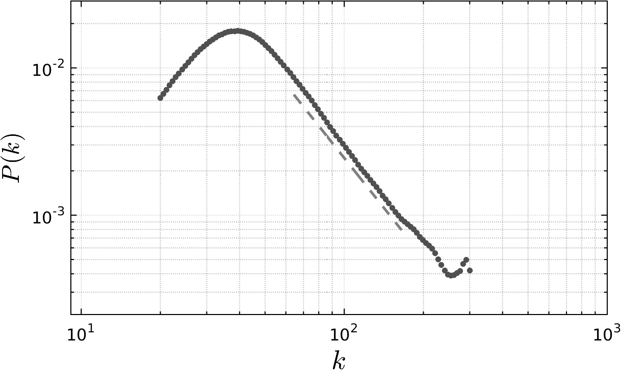
(a) (Out) degree distribution. Close to a dense condition.
Refer to caption
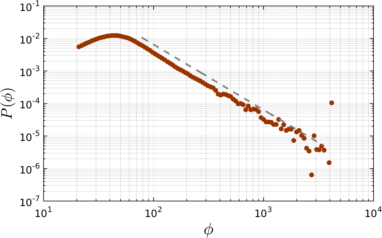
(b) (Out) strength distribution. Similar to the sparse condition.
Figure 1: Evolution of the incremental fitness model after a time of 450004500045000 steps. One can se that the degree distribution (a) is affected by the congestion effect due to the cutoff on the adjacency matrix. As for the strength distribution (b) there is no cutoff, since the connections continue to be added also to high degree nodes. In both figure we applied the density estimation in a logarithmic binning over 100 realizations. The dotted line in (b) represent the theoretical power law coefficients of Ο„=2.1𝜏2.1\tau=2.1 of the infinite limits, on the other side in dense networks as in (a) the slope of the power law coefficient is squeezed not revealing the exact power law coefficient due the upper bound degree.

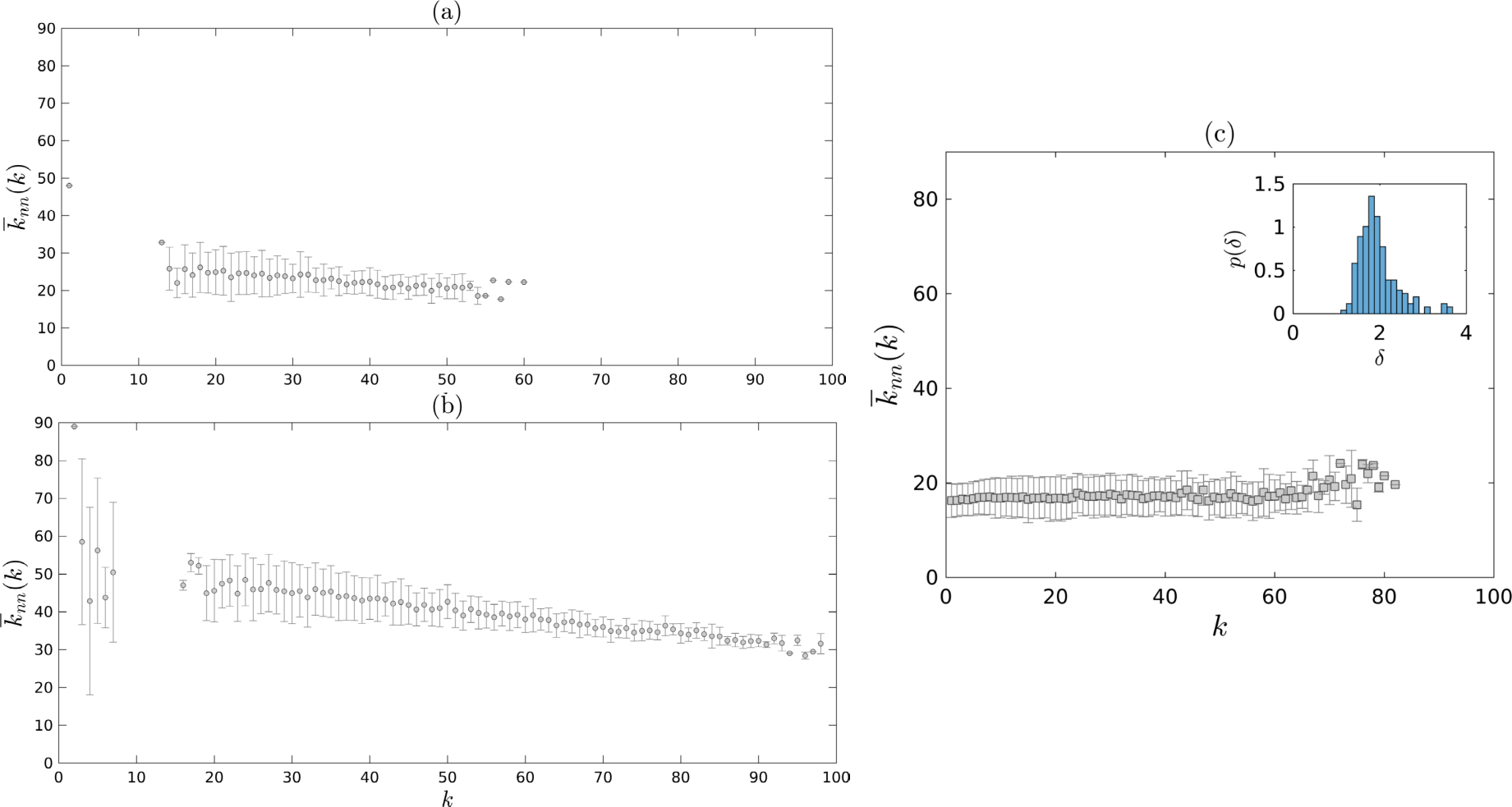
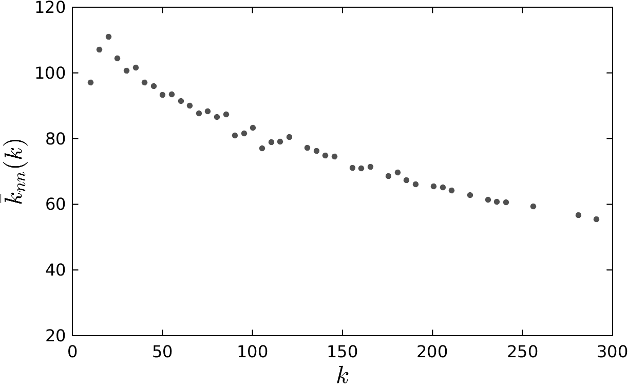
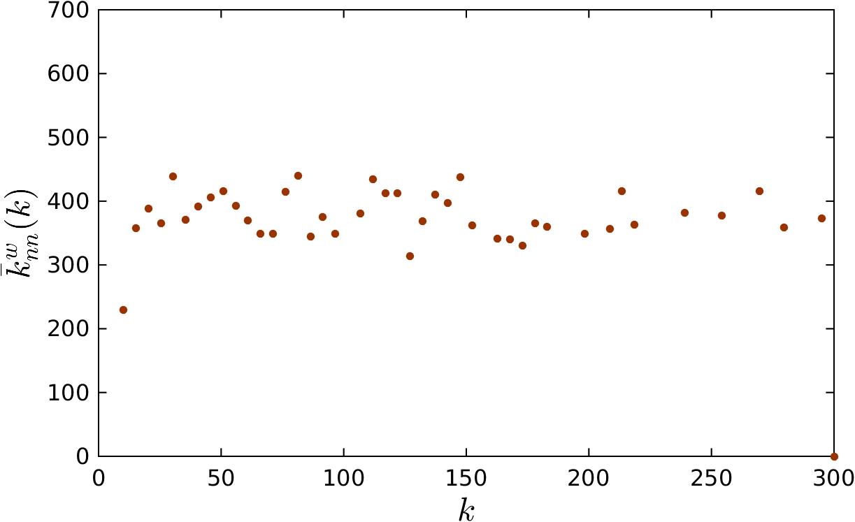
In fig.1 we can see the two distributions where the degree distribution behaves the same as in the simple graph network, while the strength does show a clear scale free behavior over the time evolution without signs of congestion. Moreover the basic structure of incremental simple graph network shows disassortativity, which is not representative of any underlying assortative or disassortative mixing. Becuase of the congestion effect, nodes with degree higher than the structural cut-off will display structural disassortativity that arises from the structure of a finite size network. Using multiple links approach, the network is no longer a simple graph, but it allows for sufficient links to maintain correlation neutrality, as showed in fig.2. If we treat the multilink network as weighted network, we can also measure the average degree of nearest neighbor degree (kΒ―n​nsubscriptΒ―π‘˜π‘›π‘›\bar{k}_{nn}) and comparing it in the version of simple graph 2(a) and in the weighted version for multi-link graph in 2(b). We used kΒ―n​nsubscriptΒ―π‘˜π‘›π‘›\bar{k}_{nn} behavior as measure of assortative structure in the network. Defining the average nearest neighbors for weighted network is Mastrandrea etΒ al., [22]:

kn​n,iw=superscriptsubscriptπ‘˜π‘›π‘›π‘–π‘€absent\displaystyle k_{nn,i}^{w}= 1Ο•iβ€‹βˆ‘j=1NAi,j​Wi​j​kj1subscriptitalic-ϕ𝑖superscriptsubscript𝑗1𝑁subscript𝐴𝑖𝑗subscriptπ‘Šπ‘–π‘—subscriptπ‘˜π‘—\displaystyle\frac{1}{\phi_{i}}\sum_{j=1}^{N}A_{i,j}W_{ij}k_{j} (32)

where Ο•isubscriptitalic-ϕ𝑖\phi_{i} is the strength of the node i𝑖i as already defined. Choosing the degree as out- or in- degrees we have two version of the average nearest neighbors degree. In order to get the average degree of nearest neighbors kΒ―n​n​(k)subscriptΒ―π‘˜π‘›π‘›π‘˜\bar{k}_{nn}(k) , we takes the average of eq.(32) over the number of nodes of strength Ο•italic-Ο•\phi. A way to double check the structural origin of the disassortative behavior of the simple graph model can be recover comparing the kΒ―n​n​(k)subscriptΒ―π‘˜π‘›π‘›π‘˜\bar{k}_{nn}(k) with a degree-preserving randomized version of itself (without multiple edges). Since there is no change in the disassortative behavior, the degree correlation pattern is not a meaningful property of the simple graph network in the incremental fitness function. On the contrary it is an artifact in the sense that it comes from a finite size effect of the model.
Refer to caption
(a) Assortative mixing property for simple graph network. Disassortative pattern in the out-degree connections.
Refer to caption
(b) Assortative mixing property for multi-link weighted network. Neutral pattern for the weighted out-degree.
Figure 2: Average degree of nearest neighbors after a time of 450004500045000 steps. It behavior is an index of degree-degree correlation through the average degree of the nearest neighbors, kn​n​(k)subscriptπ‘˜π‘›π‘›π‘˜k_{n}n(k) for nodes of (out)degree kπ‘˜k. In (a) we have a clear disassortative behavior for the simple graph procedure, and in (b) a neutral pattern as for the procedure with multi-links and the weighted version of the network.

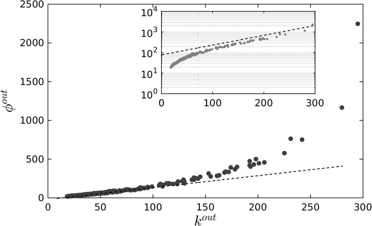
Anyway, the procedure of creating a weighted network from the accumulation of links, generates nodes’ strength that are not independent from the degree. This means that the weights are dependent of the network topology Barrat etΒ al., [1], in fact im the absence of correlation the strength should grows linearly with the degree: Ο•βˆkproportional-toitalic-Ο•π‘˜\phi\propto k. In our weighted network this is violated as seen in Fig.3. The strength of nodes grows faster than their degree, denoting a correlation between the weight and the topological properties of the network. Therefore the two quantities does not provide the same information on the system.
Refer to caption
Figure 3: Strength- degree correlation in the multi-links version of the incremental fitness model. The strength of the nodes violates the uncorrelated condition of a linear dependence as clearly seen in the inbox insert in a semilog plot.

2.3 Simple Finite Networks

The incremental fitness model has a couple of technical and practical issues to take care. One is the computational procedure to make the network evolve in time creating new links. This determines the formation of structures in the networks that can change according to which way we consider the connections among nodes. The second aspect is about finite scale of the network. The choice of the coefficients of the linking function can bring to some apparent characteristic behaviors of degree distribution, determining different scale free regimes. The incremental version of fitness driven networks has been described through the master equation eq.(7) that takes in account the temporal evolution links formation in the network with fixed number of nodes (i.e. a non growing network model). The mathematical description makes the assumption of thermodynamic limit with an infinite network. In practical case it works in the sparse condition with Lβ‰ͺNmuch-less-than𝐿𝑁L\ll N. For longer times we encounter the presence of multi-links that if forbidden brings to a congestion for high degree nodes and a network that become denser over time. Recent empirical observation put emphasis on the importance of link congestion effect in networks in which density of links increases during its evolution and the total number of links grows faster than the number of nodes:

L​(t)∝F​(N​(t),t)a,proportional-to𝐿𝑑𝐹superscriptπ‘π‘‘π‘‘π‘ŽL(t)\propto F\left(N(t),t\right)^{a}, (33)

where N𝑁N is number of nodes at time t𝑑t, and L𝐿L the number of edges at time t𝑑t. The coefficient aπ‘Ža is also the densification exponents. A particular choice of function F𝐹F in our model is for N𝑁N fixed over time and a=1π‘Ž1a=1, so we have L​(t)=t𝐿𝑑𝑑L(t)=t. In growing networks, also vertices are created so the function F𝐹F can be of the form of L​(t)∝N​(t)aproportional-to𝐿𝑑𝑁superscriptπ‘‘π‘ŽL(t)\propto N(t)^{a} , and in particular an important recent finds Leskovec etΒ al., [21] gives the definition of densification phenomena777usually the definition includes both the power law behavior of number of links, both the shrinking behavior of the network diameter. where a>1π‘Ž1a>1. In these empirical observations this phenomenon has been observed in societies and online communities as well as in the evolution of scientific fields and cities 888Among the others real examples of this phenomena are: patents citation graph, product recommendation network and large online social networks. Similar kind of phenomena are also presented in terms of accelerated growth models analytically described in Dorogovtsev and Mendes, [16] with a more tractable mathematical description. Our model is a simple and extreme model in the sense of densification effect but also focuses the attention on the effects and possible application of accelerated and densified networks. We will focus the attention on the effects of high density of two aspects of statistical features: the degree distribution and the degree degree correlations. In our case of evolution of out-degree distribution has the asymptotic form in eq.(2.1):

P​(k,t)∼c​tz​kβˆ’Ο„similar-toπ‘ƒπ‘˜π‘‘π‘superscript𝑑𝑧superscriptπ‘˜πœP(k,t)\sim c\;t^{z}\,k^{-\tau} (34)

where z=(ΞΌβˆ’1)/Ξ±π‘§πœ‡1𝛼z=(\mu-1)/\alpha for the out-degree probability, and c𝑐c is the proportional coefficient coming from the types of fitness distribution. We also exchange L𝐿L with t𝑑t since in our model L=t𝐿𝑑L=t. In order to have an estimation of the natural restrictions, one can impose two conditions to have the low and high degree region of the power law Bornholdt and Schuster, [6, Ch.Β 14] Dorogovtsev and Mendes, [14]. Imposing the normalization condition:

∫k0​(t)Nc​tz​kβˆ’Ο„βˆΌ1similar-tosuperscriptsubscriptsubscriptπ‘˜0𝑑𝑁𝑐superscript𝑑𝑧superscriptπ‘˜πœ1\int_{k_{0}(t)}^{N}c\,t^{z}k^{-\tau}\sim 1 (35)

where c𝑐c can be calculated for a truncated pareto fitness distribution as c∼(1/N)zsimilar-to𝑐superscript1𝑁𝑧c\sim(1/N)^{z}. The natural initial degree k0subscriptπ‘˜0k_{0} is the value from which we have the beginning of the power law behavior of the degree distribution.

As regard as the final degree, that signs the natural cut-off of the power law behavior. Imposing that the probability of nodes with k>kc​u​t​(t)π‘˜subscriptπ‘˜π‘π‘’π‘‘π‘‘k>k_{cut}(t) is of the order of 1/t1𝑑1/t:

tβ€‹βˆ«kc​u​t​(t)Nc​tz​kβˆ’Ο„βˆΌ1similar-to𝑑superscriptsubscriptsubscriptπ‘˜π‘π‘’π‘‘π‘‘π‘π‘superscript𝑑𝑧superscriptπ‘˜πœ1t\int_{k_{cut}(t)}^{N}c\,t^{z}k^{-\tau}\sim 1 (36)

The natural restriction parameters are obtained assuming that all the elements of the sample are independently drawn from the probability density P​(k)π‘ƒπ‘˜P(k). However, in real networks the degrees of the nodes are not simply independently drawn from a probability distribution P​(k)π‘ƒπ‘˜P(k), but must satisfy some topological constraints due to the network structure. It is possible to show that in order to have no correlations in the absence of multiple and self-connections, a scale-free network with degree distribution P​(k)∼kβˆ’Ο„similar-toπ‘ƒπ‘˜superscriptπ‘˜πœP(k)\sim k^{-\tau} and size N𝑁N must have a cutoff scaling called structural cutoff BogunΓ‘ etΒ al., [4]:

ks∼(⟨kβŸ©β€‹N)1/2.similar-tosubscriptπ‘˜π‘ superscriptdelimited-βŸ¨βŸ©π‘˜π‘12k_{s}\sim\left(\langle k\rangle N\right)^{1/2}. (37)

Thus, if nodes of degree kβ‰₯ksπ‘˜subscriptπ‘˜π‘ k\geq k_{s} exist, it is physically impossible to attach enough links between them to maintain the neutrality of the network. As studied by Catanzaro etΒ al., [12], this structural cutoff has the important implication that an otherwise neutral network may show disassortative degree correlations if kc​u​t>kssubscriptπ‘˜π‘π‘’π‘‘subscriptπ‘˜π‘ k_{cut}>k_{s}. This disassortativity is not a result of any microscopic property of the network, but is purely due to the structural limitations of the network. As regard with structural properties of the degree distribution, the natural cutoff has been evaluated taking in account tha the fitness distribution is a truncated Pareto-type for which we have the coefficient in eq.(34) is:

c=ρ0​r0zα≃αNz𝑐subscript𝜌0superscriptsubscriptπ‘Ÿ0𝑧𝛼similar-to-or-equals𝛼superscript𝑁𝑧c=\frac{\rho_{0}r_{0}^{z}}{\alpha}\simeq\frac{\alpha}{N^{z}} (38)

In the specific case of our simulation we calculate natural cutoffs of eqs.(35)(36)(37):

k0=subscriptπ‘˜0absent\displaystyle k_{0}= (1βˆ’Ο„)​[(Nβˆ’1)1βˆ’Ο„1βˆ’Ο„βˆ’(Nβˆ’1t)z]1βˆ’Ο„1𝜏1𝜏delimited-[]superscript𝑁11𝜏1𝜏superscript𝑁1𝑑𝑧\displaystyle\sqrt[1-\tau]{(1-\tau)\left[\frac{(N-1)^{1-\tau}}{1-\tau}-\left(\frac{N-1}{t}\right)^{z}\,\right]} (39)
kc​u​t=subscriptπ‘˜π‘π‘’π‘‘absent\displaystyle k_{cut}= (1βˆ’Ο„)​[(Nβˆ’1)1βˆ’Ο„1βˆ’Ο„βˆ’(Nβˆ’1t)zβ‹…1t]1βˆ’Ο„1𝜏1𝜏delimited-[]superscript𝑁11𝜏1πœβ‹…superscript𝑁1𝑑𝑧1𝑑\displaystyle\sqrt[1-\tau]{(1-\tau)\left[\frac{(N-1)^{1-\tau}}{1-\tau}-\left(\frac{N-1}{t}\right)^{z}\cdot\frac{1}{t}\right]} (40)
ks=subscriptπ‘˜π‘ absent\displaystyle k_{s}= LN​N=L𝐿𝑁𝑁𝐿\displaystyle\sqrt{\frac{L}{N}N}=\sqrt{L} (41)

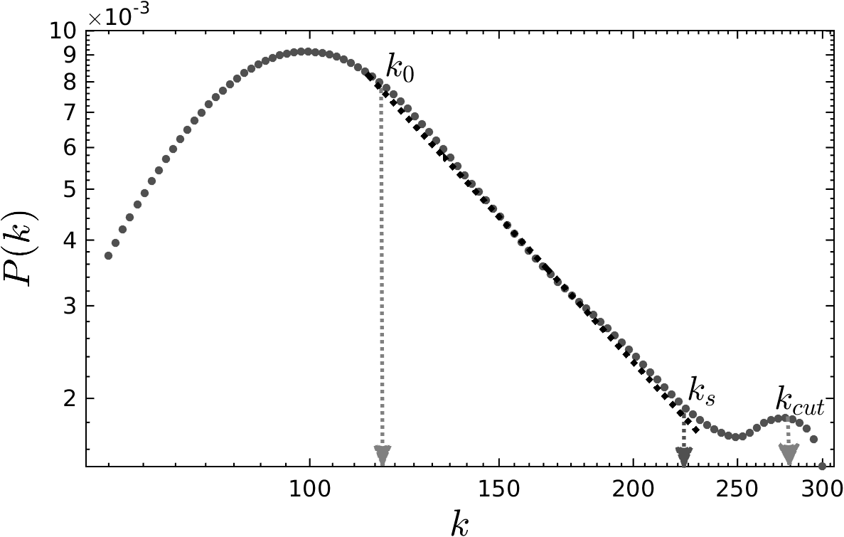
In the previous equations, if we study out-degree distributions Ο„=(Ξ±+ΞΌβˆ’1)/Ξ±πœπ›Όπœ‡1𝛼\tau=(\alpha+\mu-1)/\alpha and if we study the in-degree distribution Ο„=(Ξ²+ΞΌβˆ’1)/Ξ²πœπ›½πœ‡1𝛽\tau=(\beta+\mu-1)/\beta. An example of the estimations in the baseline case is given in fig.4, in the simple graph case where multilinks are not allowed.
Refer to caption
Figure 4: Probability density function of (out)degrees for the incremental fitness model, average over 100 realizations for density Ξ΄=50%𝛿percent50\delta=50\%, non sparse condition. The black straight dotted line represents the analytical estimation of the power law region of the out degree pdf (Ο„=2.1𝜏2.1\tau=2.1), and also the estimation of the natural restriction of (k0,kc​u​t)subscriptπ‘˜0subscriptπ‘˜π‘π‘’π‘‘(k_{0},k_{cut}) as well as the structural cutoff kssubscriptπ‘˜π‘ k_{s} in according to the analytical estimation. The evolution is made with simple graph property. The hump near kc​u​tsubscriptπ‘˜π‘π‘’π‘‘k_{cut} is due to the degree congestion where high degree nodes already reached an uniform connection probability. The value for the baseline experiment are k0β‰ˆ125subscriptπ‘˜0125k_{0}\approx 125, kc​u​tβ‰ˆ280subscriptπ‘˜π‘π‘’π‘‘280k_{cut}\approx 280 and ksβ‰ˆ232subscriptπ‘˜π‘ 232k_{s}\approx 232 as calculated via the eqs(39) (40) (41), and that corresponds what observed experimentally in the figure.

3 Properties of incremental model

In the entire discussion we have dealt with power law functions both in the probability function of fitness variables and in the degree distributions of the generated network. Once the model have been set, we want to show the usefulness of it showing how real world systems can be represented through this network. A delicate issue is the estimation of these network parameters via fitting procedures in order to generate simulations that mimics data observed in the real world as in financial markets (Bottazzi etΒ al., [8]).

Refer to caption
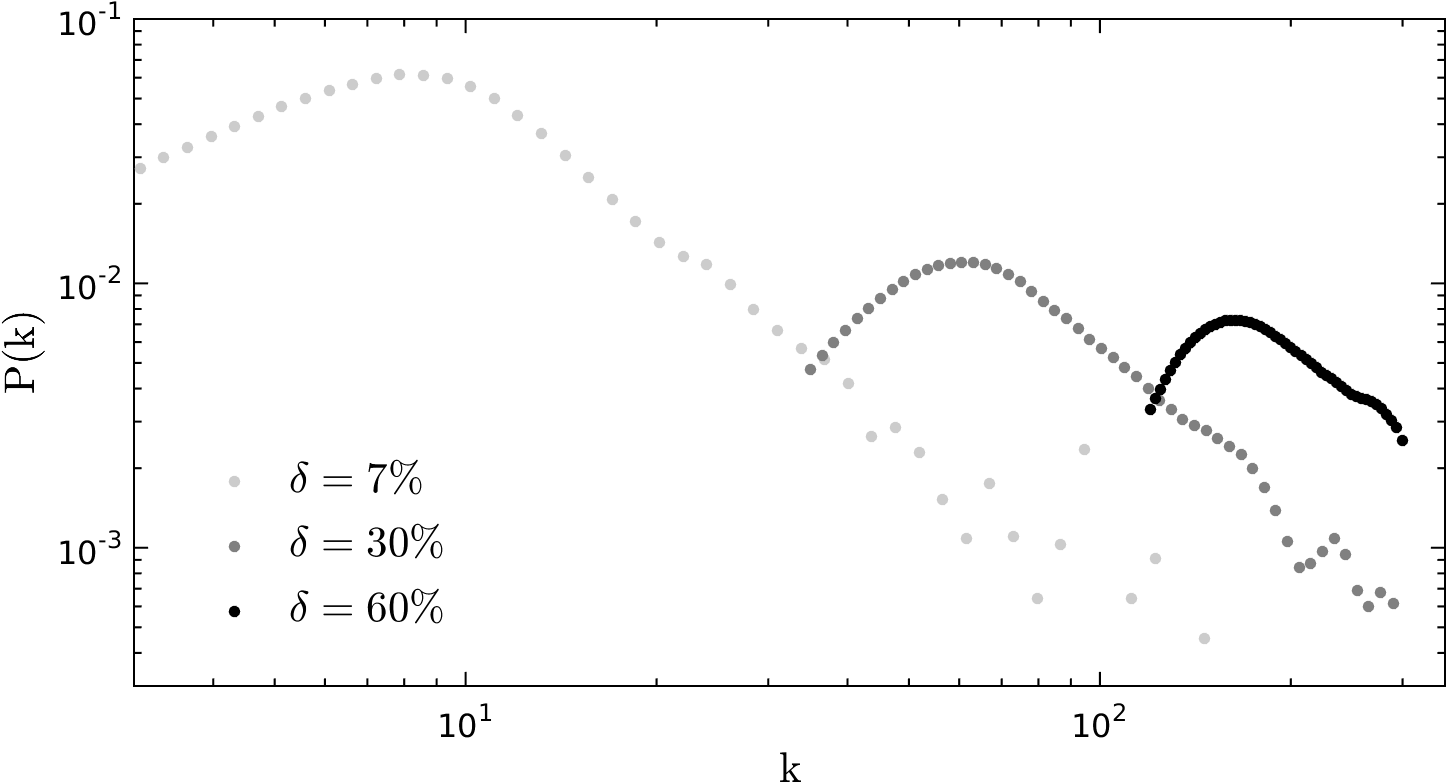
Figure 5: Probability density function of (out)degrees for the incremental fitness model for a single trajectory. The evolution excludes multi-links. Pdfs have been calculated using a logarithmic binning and a kernel density estimation with 100100100 Montecarlo replications. Each function corresponds to a different density δ𝛿\delta of the network. Increasing levels of grays corresponds to an increasing number of links where the evolution of the network last for a longer time. The asymptotic behavior is a power law distribution in the sparse condition. As the time passes and more links are added, a condensation peak appears for high degree nodes that cannot increase more their degree because of the finite size of the network.

In our simulations we used a baseline setup the model as in Table 1 where the fitness function is a truncated Pareto power law and the linking probability is a factorizable function.

Table 1: Baseline Model, the number of links changes according to the chosen average degree with L=⟨kβŸ©β€‹N𝐿delimited-βŸ¨βŸ©π‘˜π‘L=\langle k\rangle N.
Parameter Value description
N𝑁N 300300300 number of nodes
aπ‘Ža 555 fitness Pareto lower bound
b𝑏b 299299299 fitness Pareto upper bound
ΞΌπœ‡\mu 1.991.991.99 fitness Pareto coefficient
α𝛼\alpha 0.70.70.7 linking outdegree coefficient
β𝛽\beta 0.90.90.9 linking indegree coefficient
A𝐴A 299299299 maximum fitness
Ο„o​u​tsubscriptπœπ‘œπ‘’π‘‘\tau_{out} 2.412.412.41 outdegree distribution coefficient
Ο„i​nsubscriptπœπ‘–π‘›\tau_{in} 2.102.102.10 indegree distribution coefficient

Degree distribution

A concept related to the average degree is the network density δ𝛿\delta, useful to control the number of generated links in comparison to all the possible ties:

d=⟨k⟩Nβˆ’1=LN​(Nβˆ’1)𝑑delimited-βŸ¨βŸ©π‘˜π‘1𝐿𝑁𝑁1d=\frac{\langle k\rangle}{N-1}=\frac{L}{N(N-1)} (42)

well defined for finite network where the average degree is always finite. According to this index we have the sparse condition on the network if dβ‰ͺ1much-less-than𝑑1d\ll 1.

Moreover the in and out degrees are computed as:

kii​n​(t)=βˆ‘jAi,j​(t)andkio​u​t​(t)=βˆ‘jAj,i​(t)formulae-sequencesuperscriptsubscriptπ‘˜π‘–π‘–π‘›π‘‘subscript𝑗subscript𝐴𝑖𝑗𝑑andsuperscriptsubscriptπ‘˜π‘–π‘œπ‘’π‘‘π‘‘subscript𝑗subscript𝐴𝑗𝑖𝑑k_{i}^{in}(t)=\sum_{j}A_{i,j}(t)\quad\text{and}\quad k_{i}^{out}(t)=\sum_{j}A_{j,i}(t) (43)

where A𝐴A is the adjecency matrix. The average degrees are

⟨kii​n​(t)⟩=L​(t)N=⟨kio​u​t​(t)⟩.delimited-⟨⟩superscriptsubscriptπ‘˜π‘–π‘–π‘›π‘‘πΏπ‘‘π‘delimited-⟨⟩superscriptsubscriptπ‘˜π‘–π‘œπ‘’π‘‘π‘‘\langle k_{i}^{in}(t)\rangle=\frac{L(t)}{N}=\langle k_{i}^{out}(t)\rangle. (44)

The incremental fitness model generates different degree distribution along the time prescriptions of adding links that corresponds to an increase of density rate as Ξ΄=dΓ—100%𝛿𝑑percent100\delta=d\times 100\% where t=L𝑑𝐿t=L and N𝑁N is fixed. As shown if Fig.5, as time passes it is always possible to see the power law behavior of degree distribution, but the scale-free region becomes more and more restrictded while the condensation to a dense network become dominant. The dense condition is always present for high degree nodes but for strong connected network a peak shape in the tail becomes more and more evident reflecting the dense condition described in appendix A.3. A translation of the offset is due to the L𝐿L coefficient in eq.(2.1), and low degree nodes becomes more and more rare while links are added. The slope of such distribution has been evaluated according to the maximum likelihood estimation. We proved the equivalence of the degree distribution among the incremental prescription proposed here and the random prescription as in Caldarelli and Chessa, [11]. For a fitness distribution with a pareto-like distribution we found that evolutionary degree distribution eq. (2.1) coincides with the random version (calculated in appendix D, in particular eq.(116)). Throughout the paper we have always used the truncated Pareto distribution as a fitness distribution togheter with a factorizable linking function. Anyway similar results in terms of scale-free degree distribution are obtained if we use fitness values taken from a power law distribution with exponential cutoff and from exponential distribution see appendix D.2 and D.3. Anyway one should also take in account different regime behaviors of power law distributions in evaluating the fit of such distributions as discussed in the appendix E.

Isolated nodes

For practical purpose, it is important to estimate the number of nodes with zero links, which are called isolated since in the case of network contagion or failure cascades they are not affected and do not affect the system. During the incremental evolution of the networks with N𝑁N nodes, not every node has at least a connection with others nodes. We analytically estimate the average number of isolated nodes along the time, i.e for different values of average degree that is for different numbers of created links. In general, the probability that a node with fitness xπ‘₯x has degree kπ‘˜k after L𝐿L links have been created (after time t𝑑t) is given by eq.(8), so, since we are interested in the isolated nodes, we set k=0π‘˜0k=0 so can write:

px​(0|L)=(1βˆ’r0​xΞ±)Lsubscript𝑝π‘₯conditional0𝐿superscript1subscriptπ‘Ÿ0superscriptπ‘₯𝛼𝐿p_{x}(0|L)=(1-r_{0}x^{\alpha})^{L} (45)

for the outoging degree case. Knowing that our fitness distribution is a truncated power law distribution with x∈[a,b]π‘₯π‘Žπ‘x\in[a,b], we can estimate the total number of nodes with no outgoing links we can write:

Po​u​t​(0|L)=∫ab(1βˆ’r0​xΞ±)L​C​xβˆ’ΞΌβ€‹π‘‘x.subscriptπ‘ƒπ‘œπ‘’π‘‘conditional0𝐿superscriptsubscriptπ‘Žπ‘superscript1subscriptπ‘Ÿ0superscriptπ‘₯𝛼𝐿𝐢superscriptπ‘₯πœ‡differential-dπ‘₯P_{out}(0|L)=\int_{a}^{b}(1-r_{0}x^{\alpha})^{L}\;Cx^{-\mu}dx.

At this point we can use the Chebyshev theorem on the integration of binomial differentials to solve the integral

IΞ±=∫xβˆ’ΞΌβ€‹(1+β​xΞ±)L​𝑑xsubscript𝐼𝛼superscriptπ‘₯πœ‡superscript1𝛽superscriptπ‘₯𝛼𝐿differential-dπ‘₯I_{\alpha}=\int x^{-\mu}(1+\beta x^{\alpha})^{L}\,dx

and which is expressible by of the elementary functions if Lβˆˆβ„€πΏβ„€L\in\mathbb{Z}, which is our case since the total number of links L𝐿L is an integer number. Defining y=β​xΞ±/1𝑦𝛽superscriptπ‘₯𝛼1y=\beta x^{\alpha}/1 and Ξ²=βˆ’r0𝛽subscriptπ‘Ÿ0\beta=-r_{0} we can write the antiderivative as:

IΞ±=1Ξ±β€‹Ξ²βˆ’βˆ’ΞΌ+1α​B​(y;1βˆ’ΞΌΞ±,Lβˆ’1)subscript𝐼𝛼1𝛼superscriptπ›½πœ‡1𝛼𝐡𝑦1πœ‡π›ΌπΏ1I_{\alpha}={1\over\alpha}\beta^{-{-\mu+1\over\alpha}}B\left(y;{1-\mu\over\alpha},L-1\right)

where B𝐡B is the incomplete Beta Function (Chaudhry and Zubair, [13]). We can also find the probability for incoming empty nodes as IΞ²subscript𝐼𝛽I_{\beta} and then multiply the two probabilities if we want to find the case of fully isolated nodes completely disconnected from the network since they do not have any links at all. So the probability to find isolated nodes when there are L𝐿L links is given by:

P​(0,L)=𝑃0𝐿absent\displaystyle P(0,L)= ∫abpx​(0,L)​ρ​(x)​𝑑xsuperscriptsubscriptπ‘Žπ‘subscript𝑝π‘₯0𝐿𝜌π‘₯differential-dπ‘₯\displaystyle\int_{a}^{b}p_{x}(0,L)\rho(x)dx (46)
=\displaystyle=\; Iα​IΞ²subscript𝐼𝛼subscript𝐼𝛽\displaystyle I_{\alpha}I_{\beta} (47)

where we used

IΞ±=Cα​(βˆ’r0)1βˆ’ΞΌΞ±β€‹[B​(βˆ’r0​xΞ±;1βˆ’ΞΌΞ±,Lβˆ’1)]x=ax=bsubscript𝐼𝛼𝐢𝛼superscriptsubscriptπ‘Ÿ01πœ‡π›Όsuperscriptsubscriptdelimited-[]𝐡subscriptπ‘Ÿ0superscriptπ‘₯𝛼1πœ‡π›ΌπΏ1π‘₯π‘Žπ‘₯𝑏I_{\alpha}=\frac{C}{\alpha}(-r_{0})^{\frac{1-\mu}{\alpha}}\Bigg{[}B(-r_{0}x^{\alpha};\frac{1-\mu}{\alpha},L-1)\Bigg{]}_{x=a}^{x=b}

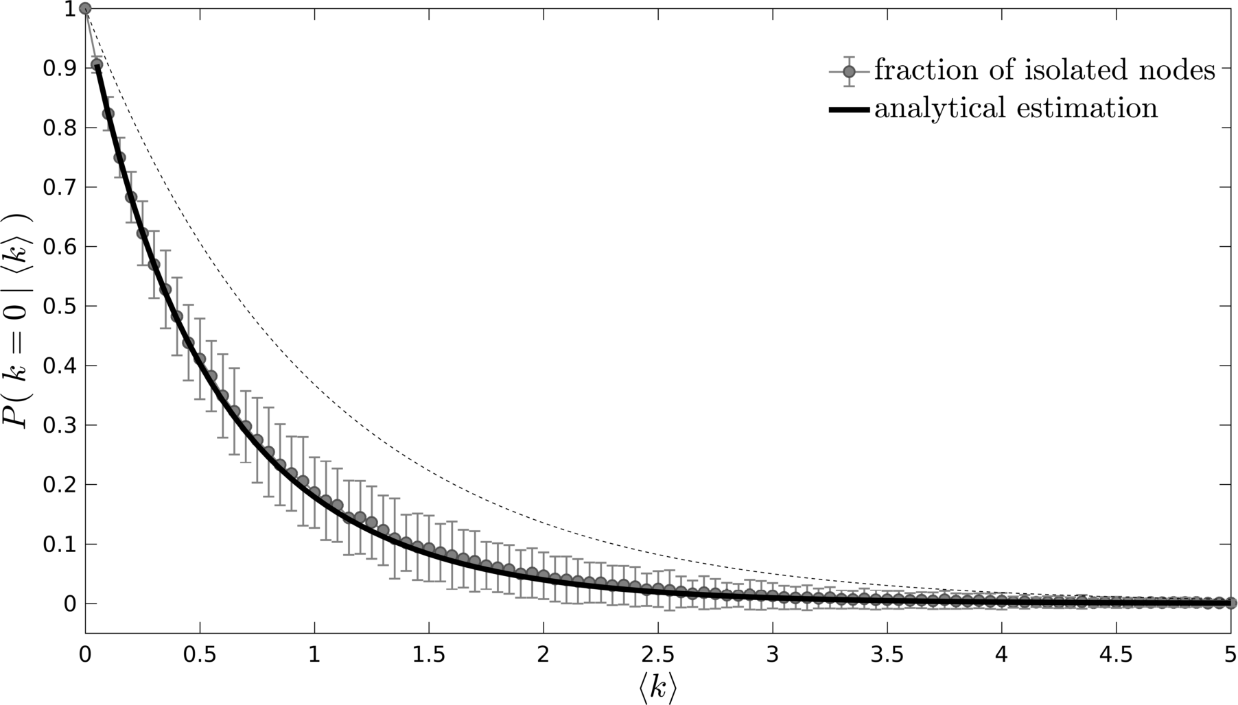
for the outoging links and similarly we define IΞ²subscript𝐼𝛽I_{\beta} for the incoming links. Then, numerically inverting this equation it is possible to know how many links we need to generates in order to have a certain percentage of isolated nodes in the network. In some practical application, it can be very useful to know the expected number of nodes with no connections at time t𝑑t, i.e. at a given average degree for the network. For example, in the case of shock propagation in network, disconnected nodes do not contribute to the cascade, in particular if selected as first step of the cascade, isolated nodes cannot trigger any shock propagation. A rough estimation of empty nodes after having L=⟨kβŸ©β€‹N𝐿delimited-βŸ¨βŸ©π‘˜π‘L=\langle k\rangle N links can be found in the random hypothesis of the probability of the allocation of undistinguished links in N𝑁N nodes (1βˆ’1/N)Lsuperscript11𝑁𝐿(1-1/N)^{L} so, the excepted fraction of isolated nodes is of the order of eβˆ’βŸ¨k⟩superscript𝑒delimited-βŸ¨βŸ©π‘˜e^{-\langle k\rangle}. We can evaluate the expected number of isolated nodes, running a Montecarlo simulations results over 100100100 realizations and compare the results with the analytical evaluation of isolated nodes after L𝐿L links with the eq.(46). We see, in Fig.6 how the analytical calculations predict the probability to find a given number of empty nodes for different values of the average degree. In contrast, the random hypothesis estimation gives very loose results at least for intermediate values of average degrees.
Refer to caption
Figure 6: Probability to find that a randomly chosen node is isolated in a network with a given average degree. This is exactly the fraction of empty nodes over the total number of nodes that is computed with a Montecarlo simulation with 100100100 repetitions, which is represented in the figure with a barplot, where the bar size is two standard deviations large. The black solid line is the analytical estimation of such fraction and the dotted gray line is the same fraction in the random graph estimation with exponential decay.

Expected number of multiple links

As a measure of difference between the multigraph and simple graph procedures, it could be useful to estimate of the expected number of multiple links in the graph. Following the combinatorial argument used by [20], the expected number of multiple links in the network is:

mΒ―m​u​l​t​i=14​(⟨k2βŸ©βˆ’βŸ¨k⟩⟨k⟩)2subscriptΒ―π‘šπ‘šπ‘’π‘™π‘‘π‘–14superscriptdelimited-⟨⟩superscriptπ‘˜2delimited-βŸ¨βŸ©π‘˜delimited-βŸ¨βŸ©π‘˜2\overline{m}_{multi}=\frac{1}{4}\left(\frac{\langle k^{2}\rangle-\langle k\rangle}{\langle k\rangle}\right)^{2} (48)

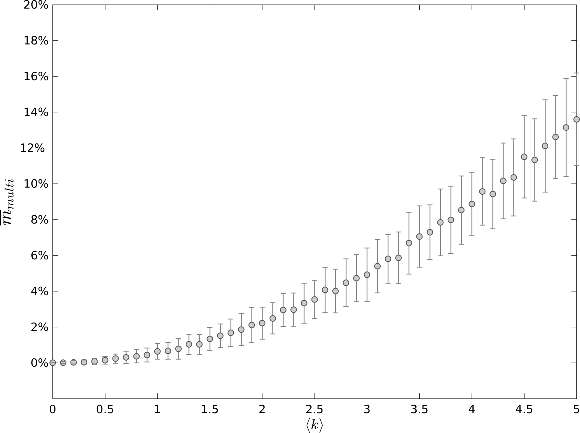
which can be verified both for out and for in degree distributions. In our baseline model the first moment of the distribution is finite, on the contrary the second moment diverges (see appendix E) so that the number of multilinks tends to increase with the number of links as seen in Fig.7 with Montecarlo simulations.
Refer to caption
Figure 7: Average fraction of multilinks in the network for different values of the average degree and so number of links in the system. The average is obtained with 100100100 replications.

Correlations and assortativity

Higher order statistics in network involve joint degree distributions and conditional probabilities that contains degree correlation information. In a directed graph, another form of degree correlation is otherwise expressed by the joint in/out-degree probability distribution function P​(𝐀)≑P​(ki​n,ko​u​t)𝑃𝐀𝑃subscriptπ‘˜π‘–π‘›subscriptπ‘˜π‘œπ‘’π‘‘P(\mathbf{k})\equiv P(k_{in},k_{out}). Let us define the transition probability Pi​n​(𝐀′|𝐀)subscript𝑃𝑖𝑛conditionalsuperscript𝐀′𝐀P_{in}(\mathbf{k}^{\prime}|\mathbf{k}) as the probability of reaching a node of degree 𝐀′superscript𝐀′\mathbf{k}^{\prime} starting from a node of degree 𝐀𝐀\mathbf{k} through an incoming link; and a similar definition for the transition probability Po​u​t​(𝐀′|𝐀)subscriptπ‘ƒπ‘œπ‘’π‘‘conditionalsuperscript𝐀′𝐀P_{out}(\mathbf{k}^{\prime}|\mathbf{k}) along an outgoing link. These transition probabilities are related through the following degree detailed balance conditions BogunΓ‘ and Serrano, [5]

ko​u​t​P​(𝐀)​Po​u​t​(𝐀′|𝐀)=ki​n′​P​(𝐀′)​Pi​n​(𝐀|𝐀′)subscriptπ‘˜π‘œπ‘’π‘‘π‘ƒπ€subscriptπ‘ƒπ‘œπ‘’π‘‘conditionalsuperscript𝐀′𝐀subscriptsuperscriptπ‘˜β€²π‘–π‘›π‘ƒsuperscript𝐀′subscript𝑃𝑖𝑛conditional𝐀superscript𝐀′k_{out}P(\mathbf{k})P_{out}(\mathbf{k}^{\prime}|\mathbf{k})=k^{\prime}_{in}P(\mathbf{k}^{\prime})P_{in}(\mathbf{k}|\mathbf{k}^{\prime}) (49)

These conditions assure that any link departing from a node, always points to another node (network closeness). We will discuss numerical behaviors of the joint degree distribution in the results P​(ki​n,ko​u​t)𝑃subscriptπ‘˜π‘–π‘›subscriptπ‘˜π‘œπ‘’π‘‘P(k_{in},k_{out}) using Montecarlo simulations. In the present discussion, the network is directed, the edges are differentiated into incoming and outgoing, so that each vertex has two coexisting degrees ki​nsubscriptπ‘˜π‘–π‘›k_{in} and ko​u​tsubscriptπ‘˜π‘œπ‘’π‘‘k_{out} , with total degree k=ki​n+ko​u​tπ‘˜subscriptπ‘˜π‘–π‘›subscriptπ‘˜π‘œπ‘’π‘‘k=k_{in}+k_{out}. Hence, the degree distribution for a directed network is a joint degree distribution P​(ko​u​t,ki​n)≑P​(𝐀)𝑃subscriptπ‘˜π‘œπ‘’π‘‘subscriptπ‘˜π‘–π‘›π‘ƒπ€P(k_{out},k_{in})\equiv P(\mathbf{k}) of in- and out-degrees that in general may be correlated. Real networks are usually correlated in the sense that the degrees of pairs of connected nodes are correlated random quantities. When two-point correlations are absent, the transition probabilities become independent of the degree of the source node, we have:

Po​u​t​(𝐀′|𝐀)=subscriptπ‘ƒπ‘œπ‘’π‘‘conditionalsuperscript𝐀′𝐀absent\displaystyle P_{out}(\mathbf{k}^{\prime}|\mathbf{k})= ki​n′​P​(𝐀′)⟨ki​n⟩subscriptsuperscriptπ‘˜β€²π‘–π‘›π‘ƒsuperscript𝐀′delimited-⟨⟩subscriptπ‘˜π‘–π‘›\displaystyle\;\frac{k^{\prime}_{in}P(\mathbf{k}^{\prime})}{\langle k_{in}\rangle} (50)
Pi​n​(𝐀′|𝐀)=subscript𝑃𝑖𝑛conditionalsuperscript𝐀′𝐀absent\displaystyle P_{in}(\mathbf{k}^{\prime}|\mathbf{k})= ko​u​t′​P​(𝐀′)⟨ko​u​t⟩subscriptsuperscriptπ‘˜β€²π‘œπ‘’π‘‘π‘ƒsuperscript𝐀′delimited-⟨⟩subscriptπ‘˜π‘œπ‘’π‘‘\displaystyle\;\frac{k^{\prime}_{out}P(\mathbf{k}^{\prime})}{\langle k_{out}\rangle} (51)

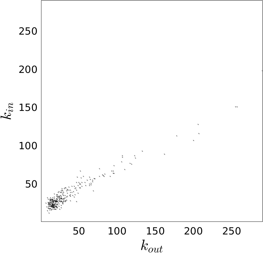
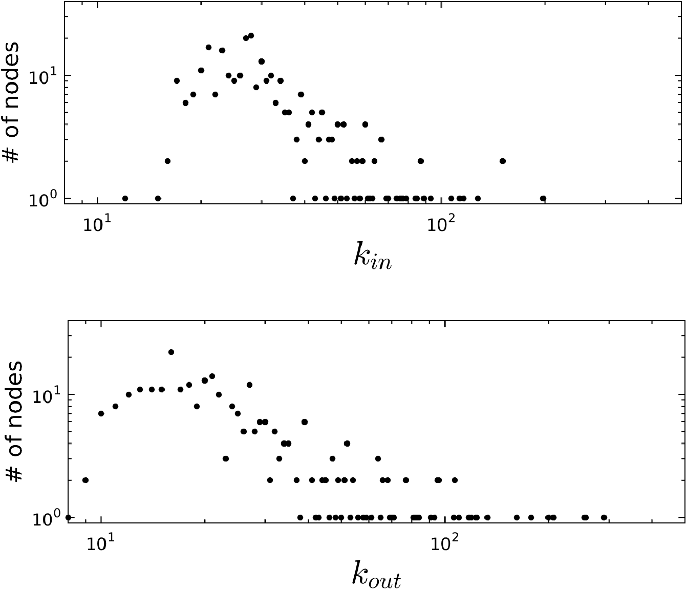
which is the case of absence of degree-degree correlations. The marginal degree distributions P​(ki​n)𝑃subscriptπ‘˜π‘–π‘›P(k_{in}) and P​(ko​u​t)𝑃subscriptπ‘˜π‘œπ‘’π‘‘P(k_{out}) involving just the in-degree and just the out-degree are a lot simpler to deal with. So, rather than dealing with the full two-dimensional degree distribution, one could just study the marginal distributions separately. In Fig.8 we apply the previous discussion to our fitness network model. We can see how the in-out joint distribution is uncorrelated and each marginal probabilities are those find in the previous sections, in particular if in the linking function Ξ±=β𝛼𝛽\alpha=\beta the points in the Fig.8(a) should stay in the diagonal. By construction, there are no correlations between a node’s in-degree and a node’s out-degree, in the sense that if one node has a large in-degree and another nodes has a small in-degree, both nodes are equally likely to have a large out-degree. The strong influence of the correlation between in- and out-degree can be seen by the fact that it determines the largest eigenvalue of the adjacency matrix Restrepo etΒ al., [24]. In our network, the assumption of uncorrelated in- and out-degrees make sense, but it certainly doesn’t have to be true in general.
Refer to caption
(a) The number of nodes in the network with given in-degree and out-degree 𝐀=(ko​u​t,ki​n)𝐀subscriptπ‘˜π‘œπ‘’π‘‘subscriptπ‘˜π‘–π‘›\mathbf{k}=(k_{out},k_{in}). This is proportional to the joint degree distribution P​(ko​u​t,ki​n)𝑃subscriptπ‘˜π‘œπ‘’π‘‘subscriptπ‘˜π‘–π‘›P(k_{out},k_{in}) which probability of a randomly picked node that has in-degree ki​nsubscriptπ‘˜π‘–π‘›k_{in} and out-degree ko​u​tsubscriptπ‘˜π‘œπ‘’π‘‘k_{out} .
Refer to caption
(b) number of nodes with given in/out degree. They indicate the marginal probabilities P​(ki​n)𝑃subscriptπ‘˜π‘–π‘›P(k_{in}) and P​(ko​u​t)𝑃subscriptπ‘˜π‘œπ‘’π‘‘P(k_{out}).
Figure 8: Degree distributions in the directed network. In (a) the bidimensional joint degree distribution, and (b) represents the marginal distribution along the direction of out and in degree, as in fig.5. In this case the density of the network is Ξ΄=7%𝛿percent7\delta=7\% and the binning is equal size without any density estimation.

Since the study of network’s response to shock a failures can only spread against the direction of links, it is necessary to obtain the fitness-conditional out-degree distribution (the propagator). As discussed in Serrano etΒ al., 2007b [27], second order statistics deals with degree-degree correlations which its empirical measurement is the average neighbour connectivity kn​n​(k)subscriptπ‘˜π‘›π‘›π‘˜k_{nn}(k), measuring the average degree of nodes neighbor of nodes with degree kπ‘˜k. A seminal work on correlations in hidden-variable networks have been done by BogunΓ‘ and Pastor-Satorras, [3] where the authors found analytical expressions for the main topological properties of these models as a function of the distribution of hidden variables and the probability of connecting nodes. As a general discussion we consider the total degree k=ki​n+ko​u​tπ‘˜subscriptπ‘˜π‘–π‘›subscriptπ‘˜π‘œπ‘’π‘‘k=k_{in}+k_{out}, so, the joint degree distribution P​(k,kβ€²)π‘ƒπ‘˜superscriptπ‘˜β€²P(k,k^{\prime}) is the probability that a randomly chosen link connects nodes of degree kπ‘˜k and kβ€²superscriptπ‘˜β€²k^{\prime}. Moreover the conditional probability P​(kβ€²|k)𝑃conditionalsuperscriptπ‘˜β€²π‘˜P(k^{\prime}|k) is the probability that if one end-node of a link is of degree kπ‘˜k, then its second end-node is of degree kβ€²superscriptπ‘˜β€²k^{\prime}. The relation of those probabilities is expressed through the degree detailed balance condition:

k​P​(kβ€²|k)​P​(k)=k′​P​(k|kβ€²)​P​(kβ€²)=⟨kβŸ©β€‹P​(k,kβ€²)π‘˜π‘ƒconditionalsuperscriptπ‘˜β€²π‘˜π‘ƒπ‘˜superscriptπ‘˜β€²π‘ƒconditionalπ‘˜superscriptπ‘˜β€²π‘ƒsuperscriptπ‘˜β€²delimited-βŸ¨βŸ©π‘˜π‘ƒπ‘˜superscriptπ‘˜β€²kP(k^{\prime}|k)P(k)=k^{\prime}P(k|k^{\prime})P(k^{\prime})=\langle k\rangle P(k,k^{\prime}) (52)

Actually, such histograms in finite size systems are highly affected by statistical fluctuations getting bad empirical evaluate of network correlations. As better characterization of degree correlations, it is then more convenient to use the mean degree of the neighbors of a node as a function of its degree kπ‘˜k. The average nearest neighbors degree (ANND), kΒ―n​n​(k)subscriptΒ―π‘˜π‘›π‘›π‘˜\bar{k}_{nn}(k), of vertices of degree kπ‘˜k is defined as a smoothed conditional probability:

kΒ―n​n​(k)=βˆ‘kβ€²k′​P​(kβ€²|k)subscriptΒ―π‘˜π‘›π‘›π‘˜subscriptsuperscriptπ‘˜β€²superscriptπ‘˜β€²π‘ƒconditionalsuperscriptπ‘˜β€²π‘˜\bar{k}_{nn}(k)=\sum_{k^{\prime}}k^{\prime}P(k^{\prime}|k) (53)

so that the statistical fluctuations of P​(kβ€²|k)𝑃conditionalsuperscriptπ‘˜β€²π‘˜P(k^{\prime}|k) results to be more dumped. In the case of incremental fitness driven networks, we have the hidden variable xπ‘₯x that represents a property of that node influencing its ability to make links. In our case of fitness driven network BogunΓ‘ and Pastor-Satorras, [3], Serrano etΒ al., 2007a [26], Servedio etΒ al., [28] let us define the conditional average degree of the nearest neighbors of a node of fitness xπ‘₯x as:

kn​n​(x)=βˆ«π‘‘x′​k​(xβ€²)​ϕ​(xβ€²|x),subscriptπ‘˜π‘›π‘›π‘₯differential-dsuperscriptπ‘₯β€²π‘˜superscriptπ‘₯β€²italic-Ο•conditionalsuperscriptπ‘₯β€²π‘₯k_{nn}(x)=\int dx^{\prime}\,k(x^{\prime})\phi(x^{\prime}|x), (54)

where ϕ​(xβ€²|x)italic-Ο•conditionalsuperscriptπ‘₯β€²π‘₯\phi(x^{\prime}|x) is the conditional probability that a node of fitness xπ‘₯x is connected to a node of fitness xβ€²superscriptπ‘₯β€²x^{\prime}:

ϕ​(xβ€²|x)=ρ​(xβ€²)​f​(x,xβ€²)βˆ«π‘‘x′′​ρ​(xβ€²β€²)​f​(x,xβ€²β€²)=N​ρ​(xβ€²)​f​(x,xβ€²)k​(x)italic-Ο•conditionalsuperscriptπ‘₯β€²π‘₯𝜌superscriptπ‘₯′𝑓π‘₯superscriptπ‘₯β€²differential-dsuperscriptπ‘₯β€²β€²πœŒsuperscriptπ‘₯′′𝑓π‘₯superscriptπ‘₯β€²β€²π‘πœŒsuperscriptπ‘₯′𝑓π‘₯superscriptπ‘₯β€²π‘˜π‘₯\phi(x^{\prime}|x)=\frac{\rho(x^{\prime})\,f(x,x^{\prime})}{\int{dx^{{}^{\prime\prime}}}\rho(x^{{}^{\prime\prime}})\,f(x,x^{{}^{\prime\prime}})}=\frac{N\rho(x^{\prime})f(x,x^{\prime})}{k(x)} (55)

that it the probability of finding a node of fitness xβ€²superscriptπ‘₯β€²x^{\prime} times the probability of creating such link. Thus, one has that

kn​n​(x)=Nk​(x)β€‹βˆ«π‘‘x′​ρ​(xβ€²)​k​(xβ€²)​f​(x,xβ€²)subscriptπ‘˜π‘›π‘›π‘₯π‘π‘˜π‘₯differential-dsuperscriptπ‘₯β€²πœŒsuperscriptπ‘₯β€²π‘˜superscriptπ‘₯′𝑓π‘₯superscriptπ‘₯β€²k_{nn}(x)=\frac{N}{k(x)}\int dx^{\prime}\,\rho(x^{\prime})k(x^{\prime})f(x,x^{\prime}) (56)

so the correlation function of average degree of nearest neighbor (ANND) is:

kn​n​(k)=1+1P​(k)β€‹βˆ«π‘‘x​ρ​(x)​pL​(k|x)​kn​n​(x)subscriptπ‘˜π‘›π‘›π‘˜11π‘ƒπ‘˜differential-dπ‘₯𝜌π‘₯subscript𝑝𝐿conditionalπ‘˜π‘₯subscriptπ‘˜π‘›π‘›π‘₯k_{nn}(k)=1+\frac{1}{P(k)}\int dx\,\rho(x)p_{L}(k|x)k_{nn}(x) (57)

where the propagator pL​(k|x)subscript𝑝𝐿conditionalπ‘˜π‘₯p_{L}(k|x) has been found in our case to fulfill the poissonian distribution999 One can also define the probability that a node of actual degree kπ‘˜k has associated a fitness xπ‘₯x is called pLβˆ—β€‹(x|k)superscriptsubscript𝑝𝐿conditionalπ‘₯π‘˜p_{L}^{*}(x|k) that is the inverse of the propagator in the master equation eq.(7), and it is defined via the Bayes’ formula: P​(k)​pLβˆ—β€‹(x|k)=ρ​(x)​pL​(k|x)π‘ƒπ‘˜superscriptsubscript𝑝𝐿conditionalπ‘₯π‘˜πœŒπ‘₯subscript𝑝𝐿conditionalπ‘˜π‘₯P(k)\,p_{L}^{*}(x|k)=\rho(x)\,p_{L}(k|x) of eq.(9). Rewriting the eq.(55) we can write for the out-degree case:

kn​n​(x)=subscriptπ‘˜π‘›π‘›π‘₯absent\displaystyle k_{nn}(x)= Nk0​xΞ±β€‹βˆ«π‘‘x′​k0​x′⁣α​C​xβ€²β£βˆ’ΞΌβ€‹xα​x′⁣βAΞ±+β𝑁subscriptπ‘˜0superscriptπ‘₯𝛼differential-dsuperscriptπ‘₯β€²subscriptπ‘˜0superscriptπ‘₯′𝛼𝐢superscriptπ‘₯β€²πœ‡superscriptπ‘₯𝛼superscriptπ‘₯′𝛽superscript𝐴𝛼𝛽\displaystyle\frac{N}{k_{0}x^{\alpha}}\int dx^{\prime}\,k_{0}x^{\prime\alpha}\,Cx^{\prime-\mu}\,\frac{x^{\alpha}x^{\prime\beta}}{A^{\alpha+\beta}}
=\displaystyle= N​CAΞ±+Ξ²β€‹βˆ«abx′⁣α+Ξ²βˆ’ΞΌβ€‹π‘‘x′𝑁𝐢superscript𝐴𝛼𝛽superscriptsubscriptπ‘Žπ‘superscriptπ‘₯β€²π›Όπ›½πœ‡differential-dsuperscriptπ‘₯β€²\displaystyle\frac{NC}{A^{\alpha+\beta}}\int_{a}^{b}x^{\prime\alpha+\beta-\mu}dx^{\prime}
=\displaystyle= N​CAΞ±+β​xΞ±+Ξ²βˆ’ΞΌ+1Ξ±+Ξ²βˆ’ΞΌ+1|x=ax=bevaluated-at𝑁𝐢superscript𝐴𝛼𝛽superscriptπ‘₯π›Όπ›½πœ‡1π›Όπ›½πœ‡1π‘₯π‘Žπ‘₯𝑏\displaystyle\frac{NC}{A^{\alpha+\beta}}\frac{x^{\alpha+\beta-\mu+1}}{\alpha+\beta-\mu+1}\Bigg{|}_{x=a}^{x=b}
=:absent:\displaystyle=: K0subscript𝐾0\displaystyle K_{0}

which yields the ANND function to be:

kΒ―n​n​(k)=subscriptΒ―π‘˜π‘›π‘›π‘˜absent\displaystyle\overline{k}_{nn}(k)= 1+K0P​(k)β€‹βˆ«π‘‘x​ρ​(x)​pL​(k|x)1subscript𝐾0π‘ƒπ‘˜differential-dπ‘₯𝜌π‘₯subscript𝑝𝐿conditionalπ‘˜π‘₯\displaystyle 1+\frac{K_{0}}{P(k)}\int dx\rho(x)p_{L}(k|x)
=\displaystyle= 1+K01subscript𝐾0\displaystyle 1+K_{0}

which is independent of kπ‘˜k, a signature of lack of correlations. The same is valid we choose the in-degree ANND choosing ν​(x)=r0​xβ𝜈π‘₯subscriptπ‘Ÿ0superscriptπ‘₯𝛽\nu(x)=r_{0}x^{\beta} and k​(x)=k0​xΞ²π‘˜π‘₯subscriptπ‘˜0superscriptπ‘₯𝛽k(x)=k_{0}x^{\beta} . Despite the fact that the ANND is not a exhaustive measure of degree-correlations, it gives is widely used to measure dependencies between degrees of neighbor nodes in a network. It is worth to notice that this is a result of our specific choice of the linking function, in fact, other choices , for example a threshold function, brings to natural assortative or disassortative behaviors despite the fact that the degree distributions are scale free. The assortativity mixing is expressed by the average nearest neighbor degree, computed as:

kn​n,i=1kiβ€‹βˆ‘jβˆˆΞ˜β€‹(i)kj=1kiβ€‹βˆ‘jβ‰ i,1NAi​j​kjsubscriptπ‘˜π‘›π‘›π‘–1subscriptπ‘˜π‘–subscriptπ‘—Ξ˜π‘–subscriptπ‘˜π‘—1subscriptπ‘˜π‘–superscriptsubscript𝑗𝑖1𝑁subscript𝐴𝑖𝑗subscriptπ‘˜π‘—k_{nn,i}=\frac{1}{k_{i}}\sum_{j\in\varTheta(i)}k_{j}=\frac{1}{k_{i}}\sum_{j\neq i,1}^{N}A_{ij}k_{j} (58)

where kisubscriptπ‘˜π‘–k_{i} is the degree of node i𝑖i and Ξ˜β€‹(i)Ξ˜π‘–\varTheta(i) are the neighbors of node i𝑖i. Then the ANND function can be computed as the average value of eq.(58) over all the node with a certain degree kπ‘˜k. In the directed graph case, we split the ANND for both incoming and outgoing links as Squartini and Garlaschelli, [29]:

kn​n,io​u​t=superscriptsubscriptπ‘˜π‘›π‘›π‘–π‘œπ‘’π‘‘absent\displaystyle k_{nn,i}^{out}= βˆ‘jβ‰ iβˆ‘kβ‰ jAi​j​Aj​kβˆ‘jβ‰ iAi​jsubscript𝑗𝑖subscriptπ‘˜π‘—subscript𝐴𝑖𝑗subscriptπ΄π‘—π‘˜subscript𝑗𝑖subscript𝐴𝑖𝑗\displaystyle\;\frac{\sum_{j\neq i}\sum_{k\neq j}A_{ij}A_{jk}}{\sum_{j\neq i}A_{ij}} (59)
kn​n,ii​n=superscriptsubscriptπ‘˜π‘›π‘›π‘–π‘–π‘›absent\displaystyle k_{nn,i}^{in}= βˆ‘jβ‰ iβˆ‘kβ‰ jAj​i​Ak​jβˆ‘jβ‰ iAj​isubscript𝑗𝑖subscriptπ‘˜π‘—subscript𝐴𝑗𝑖subscriptπ΄π‘˜π‘—subscript𝑗𝑖subscript𝐴𝑗𝑖\displaystyle\;\frac{\sum_{j\neq i}\sum_{k\neq j}A_{ji}A_{kj}}{\sum_{j\neq i}A_{ji}} (60)

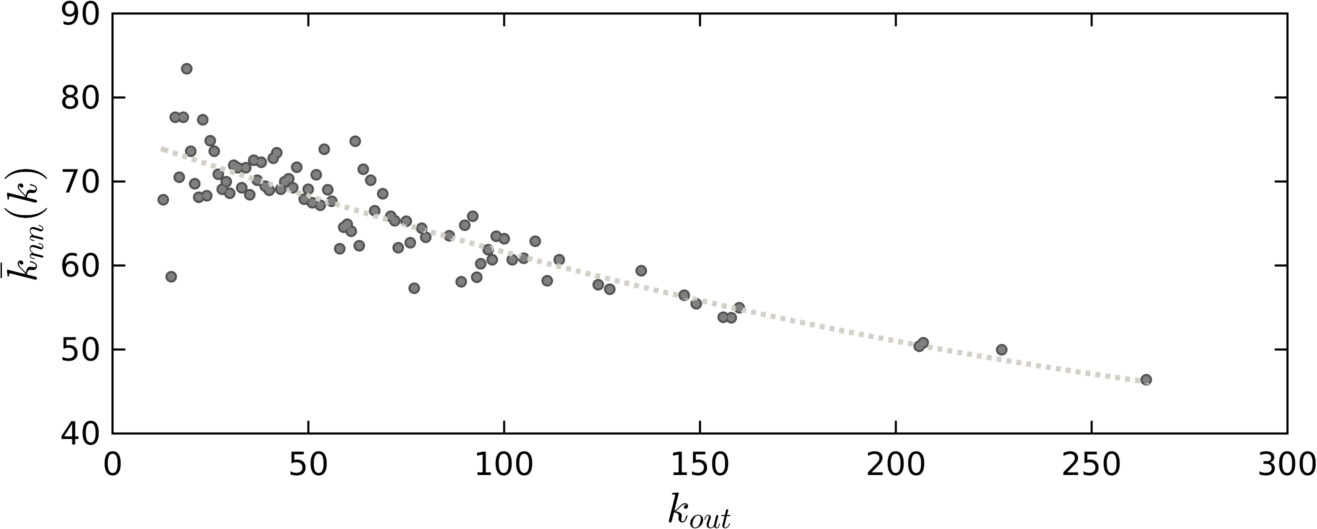
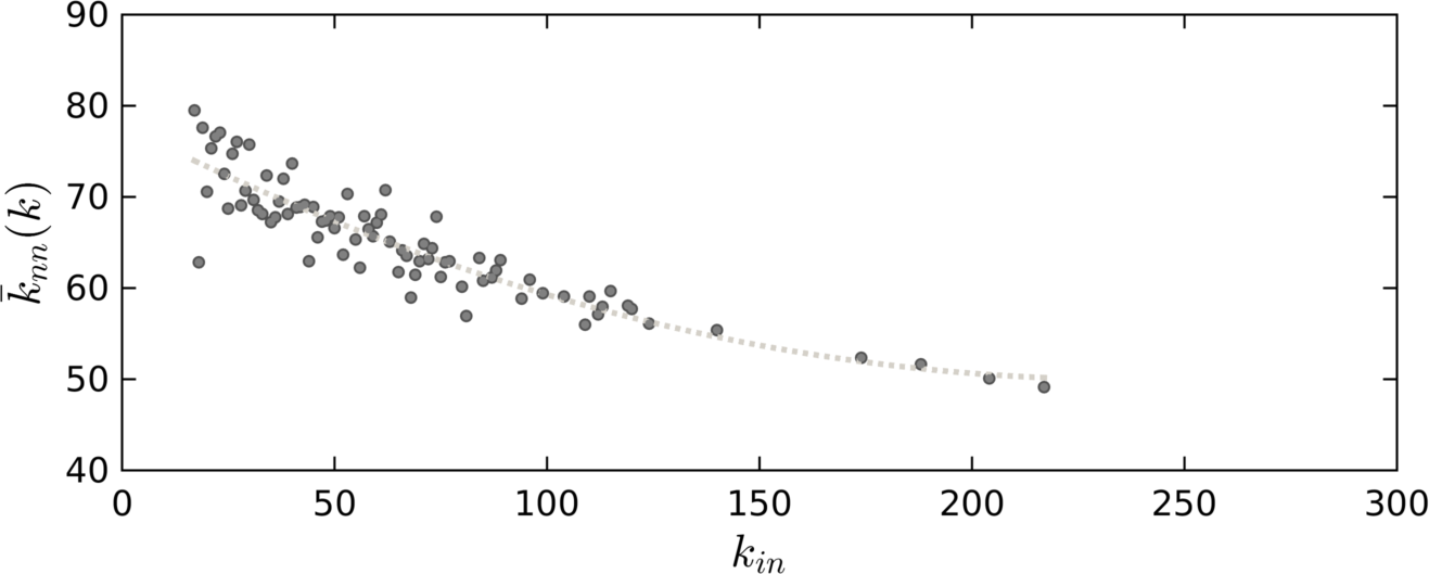
From the simulations over 100100100 repetitions from Fig.9 we observe a disassortative behavior of our baseline network which is in contrast with the neutral mixing predicted by the analytical calculations. We will devote the next section to the discussion of this behavior in terms of finite-size effects.
Refer to caption
(a) Outgoing ANND
Refer to caption
(b) Incoming ANND
Figure 9: Average degree of nearest neighbors and disassortative behavior of the incremental fitness model in our baseline but in a very dense network with 45000 links (Ξ΄=50%𝛿percent50\delta=50\%).

The fact that fitness model with factorizable linking function does not have any assortative behavior, derives from a derivation in which the system is closer to its more plausible configuration which correspond to run our incremental formulation up to a time for which we get the average degree of the random version in the thermodynamic limit (Nβ†’βˆžβ†’π‘N\to\infty). One of the most important applications of hidden variable model is that of creating network with a given degree correlation Vespignani and Caldarelli, [30], and one of the simplest example is one for which a threshold linking function is chosen, as shown in BogunΓ‘ and Pastor-Satorras, [3]. A comparison between the incremental procedure and the random version, can be useful to highlight the fact that there is a strong (apparent) discrepancy between the two generative prescriptions of the network. Since in the random model is not possible tho choose a given number of links (so the density), each simulation gives a different average degree which fluctuates around the expected value (as calculated in appendix D.1 for the case of truncated power law fitness distribution.). As consequences the ANND function shows a clear neutral assortativity as predicted by the theoretical calculations. As shown in Fig.10 the incremental version allows to observe the assortative behavior for different replications with the same number of links. More the network is dense more the the ANND shows its spurious disassortativity due to the effect of finite size of the system. Anyway everything turns to coincide to the theoretical prediction for Nβ†’βˆžβ†’π‘N\to\infty.

Refer to caption
Figure 10: ANND function in the incremental model (a) and (b) and in the random model (c) over averaged over 200200200 Montecarlo replications. In particular: (a) the network is run up to reach a density of Ξ΄=10%𝛿percent10\delta=10\% where the assortativity is almost neutral within the the error bars. (b) the network reached a density of Ξ΄=20%𝛿percent20\delta=20\% where the disassortativy behavior is more evident. On the contrary, in the random model the network, replicated 200200200 times, shows a δ𝛿\delta varying according the random configuration reached for each replication. So δ𝛿\delta is distributed according to the inset in the figure and the assortative mixing results to be neutral. Actually, for single realizations, the two models show the same spurious disassortativity for finite networks.

4 Conclusions

In this paper we address some theoretical interesting features of scale free networks with an hidden variable structure, focusing on a incremental interpretation of the model. We gave a wave-like analytical description of the network dynamics which van be easily generalized for different choices of fitness distribution and pair linking function. Moreover this approach is useful to stress the importance of finite-size effects as the arise of correlations in not-infinite systems. As regard to some practical issues, the advantage of such procedure respect to the random generative procedure is the possibility to create a network with a desired number of links (i.e. average degree) in the network. This approach tunrs to be useful in simulations of contagion and cascades simulations in the theoretical and empirical stdies of financial networks where system with different degrees of inter-connectivity is chosen to simulate different scenarios of systemic risks. The fact of having a incremental procedure allows also to save time in the computational selections of parameters for the contagion and cascade dynamics. Moreover we can understand how some selections of linking probability can give birth of spurious degree-correlations due to the finite size of the network. Ultimately a weighted version of the model is provided which solves the limitation of the theoretical description in a non sparse networks.

Acknowledgement

Fabio Vanni acknowledges support from the European Union’s Horizon 2020 research and innovation programme under grant agreement No.822781 GROWINPRO - Growth Welfare Innovation Productivity.

APPENDICES

Appendix A Solution to the Master Equation

In the following section we describe three different ways to solve the master equation of the kinetic fitness network. In all the solutions the function r​(x)π‘Ÿπ‘₯r(x) that depends on the fitness variable is not involved in the procedure until the integration for the total degree distribution. In this section we have to consider the couple of variables (k,t)π‘˜π‘‘(k,t) that is the degree of a node and the time of network evolution that express also the number of created links up the that time. We will use in sequential section the discrete-degree and discrete-time approach, then the discrete-degree and continuous-time approach, and finally the continuous-degree and continuous-time approach. The original master equation for the evolution of the conditional-fitness probabilities is:

pt+1​(k|x)=subscript𝑝𝑑1conditionalπ‘˜π‘₯absent\displaystyle p_{t+1}(k|x)= [1βˆ’r​(x)]​pt​(k|x)+r​(x)​pt​(kβˆ’1|x),delimited-[]1π‘Ÿπ‘₯subscript𝑝𝑑conditionalπ‘˜π‘₯π‘Ÿπ‘₯subscriptπ‘π‘‘π‘˜conditional1π‘₯\displaystyle\;\big{[}1-r(x)\big{]}\,p_{t}(k|x)+r(x)\,p_{t}(k-1|x), (61)

taking in account the initial condition pt=0​(k|x)=Ξ΄0,ksubscript𝑝𝑑0conditionalπ‘˜π‘₯subscript𝛿0π‘˜p_{t=0}(k|x)=\delta_{0,k}.

A.1 Discrete solution

We consider discrete time step and discrete degree, as the most suitable case of network evolution. Let us take discrete time steps 1 of t=L𝑑𝐿t=L. Identifying the time with the number of links added:

{pt​(k|x)=(1βˆ’r​(x))​pt​(k|x)+r​(x)​pt​(kβˆ’1|x)for ​kβ‰₯1pt​(0|x)=(1βˆ’r​(x))​pt​(0|x)casesformulae-sequencesubscript𝑝𝑑conditionalπ‘˜π‘₯1π‘Ÿπ‘₯subscript𝑝𝑑conditionalπ‘˜π‘₯π‘Ÿπ‘₯subscriptπ‘π‘‘π‘˜conditional1π‘₯forΒ π‘˜1missing-subexpressionsubscript𝑝𝑑conditional0π‘₯1π‘Ÿπ‘₯subscript𝑝𝑑conditional0π‘₯missing-subexpression\left\{\begin{array}[]{l l}p_{t}(k|x)=\big{(}1-r(x)\big{)}\,p_{t}(k|x)+r(x)\,p_{t}(k-1|x)\qquad\text{for }k\geq 1\\ p_{t}(0|x)=\big{(}1-r(x)\big{)}\,p_{t}(0|x)\end{array}\right. (62)

with initial condition p0​(k|x)=Ξ΄0,ksubscript𝑝0conditionalπ‘˜π‘₯subscript𝛿0π‘˜p_{0}(k|x)=\delta_{0,k}. Considering the generating function for kβ‰₯1π‘˜1k\geq 1:

G​(s,k)=βˆ‘t=0∞st​pt​(k|x)πΊπ‘ π‘˜superscriptsubscript𝑑0superscript𝑠𝑑subscript𝑝𝑑conditionalπ‘˜π‘₯G(s,k)=\sum_{t=0}^{\infty}s^{t}p_{t}(k|x)

multiplying both sides of eq.(62) by stsuperscript𝑠𝑑s^{t} and summing over t𝑑t:

βˆ‘t=0∞st​pt​(k|x)=(1βˆ’r​(x))β€‹βˆ‘t=0∞st​pt​(k|x)+r​(x)β€‹βˆ‘t=0∞st​pt​(kβˆ’1|x)superscriptsubscript𝑑0superscript𝑠𝑑subscript𝑝𝑑conditionalπ‘˜π‘₯1π‘Ÿπ‘₯superscriptsubscript𝑑0superscript𝑠𝑑subscript𝑝𝑑conditionalπ‘˜π‘₯π‘Ÿπ‘₯superscriptsubscript𝑑0superscript𝑠𝑑subscriptπ‘π‘‘π‘˜conditional1π‘₯\sum_{t=0}^{\infty}s^{t}p_{t}(k|x)=(1-r(x))\sum_{t=0}^{\infty}s^{t}p_{t}(k|x)+r(x)\sum_{t=0}^{\infty}s^{t}p_{t}(k-1|x)

the l.h.s is equivalent to:

1sβ€‹βˆ‘t=0∞st+1​pt+1​(k|x)=1sβ€‹βˆ‘t=1∞st​pt​(k|x)=1s​(G​(s,k)βˆ’p0​(k|x))1𝑠superscriptsubscript𝑑0superscript𝑠𝑑1subscript𝑝𝑑1conditionalπ‘˜π‘₯1𝑠superscriptsubscript𝑑1superscript𝑠𝑑subscript𝑝𝑑conditionalπ‘˜π‘₯1π‘ πΊπ‘ π‘˜subscript𝑝0conditionalπ‘˜π‘₯\frac{1}{s}\sum_{t=0}^{\infty}s^{t+1}p_{t+1}(k|x)=\frac{1}{s}\sum_{t=1}^{\infty}s^{t}p_{t}(k|x)=\frac{1}{s}(G(s,k)-p_{0}(k|x))

and the equation reduces to:

1s​(G​(s,k)βˆ’p0​(k|x))=(1βˆ’r​(x))​G​(s,k)+r​G​(s,kβˆ’1).1π‘ πΊπ‘ π‘˜subscript𝑝0conditionalπ‘˜π‘₯1π‘Ÿπ‘₯πΊπ‘ π‘˜π‘ŸπΊπ‘ π‘˜1\frac{1}{s}(G(s,k)-p_{0}(k|x))=(1-r(x))\,G(s,k)+r\,G(s,k-1).

Since p0​(k|x)=0subscript𝑝0conditionalπ‘˜π‘₯0p_{0}(k|x)=0 and collecting common terms:

G​(s,k)=r​(x)​s1βˆ’s​(1βˆ’r​(x))​G​(s,kβˆ’1)πΊπ‘ π‘˜π‘Ÿπ‘₯𝑠1𝑠1π‘Ÿπ‘₯πΊπ‘ π‘˜1G(s,k)=\frac{r(x)\,s}{1-s(1-r(x))}G(s,k-1)

If k=0π‘˜0k=0 it is

1s​(G​(s,0)βˆ’p0​(0,x))=(1βˆ’r​(x))​G​(s,0)1𝑠𝐺𝑠0subscript𝑝00π‘₯1π‘Ÿπ‘₯𝐺𝑠0\frac{1}{s}(G(s,0)-p_{0}(0,x))=(1-r(x))G(s,0)

and since p0​(0,x)=1subscript𝑝00π‘₯1p_{0}(0,x)=1

G​(s,0)=11βˆ’s​(1βˆ’r​(x))𝐺𝑠011𝑠1π‘Ÿπ‘₯G(s,0)=\frac{1}{1-s(1-r(x))}

so that in general

G​(s,k)=sk​r​(x)k(1βˆ’s​(1βˆ’r​(x)))k+1πΊπ‘ π‘˜superscriptπ‘ π‘˜π‘Ÿsuperscriptπ‘₯π‘˜superscript1𝑠1π‘Ÿπ‘₯π‘˜1G(s,k)=\frac{s^{k}r(x)^{k}}{(1-s(1-r(x)))^{k+1}} (63)

Notice that

pt(k,x)=1t!dtd​stG(s,k)|s=0p_{t}(k,x)=\frac{1}{t!}\;\frac{d^{t}}{d\,s^{t}}G(s,k)\Big{\rvert}_{s=0}

when taking the t𝑑t derivative of eq.(63) computed in s=0𝑠0s=0, the result is zero if t<kπ‘‘π‘˜t<k. In general

dtd​stG(s,k)|s=0=\displaystyle\frac{d^{t}}{d\,s^{t}}G(s,k)\Big{\rvert}_{s=0}= r(x)kβˆ‘n=0t(tn)dnd​snsk|s=0\displaystyle r(x)^{k}\sum_{n=0}^{t}{{t}\choose{n}}\frac{d^{n}}{d\,s^{n}}s^{k}\Bigg{\rvert}_{s=0}
dtβˆ’nd​stβˆ’n1(1βˆ’s​(1βˆ’r​(x)))k+1|s=0\displaystyle\frac{d^{t-n}}{d\,s^{t-n}}\frac{1}{(1-s(1-r(x)))^{k+1}}\Bigg{\rvert}_{s=0}

but the first term is different from zero only if n=kπ‘›π‘˜n=k, then:

pt​(k,x)=subscriptπ‘π‘‘π‘˜π‘₯absent\displaystyle p_{t}(k,x)= 1t!dtd​stG(s,k)|s=0\displaystyle\frac{1}{t!}\;\frac{d^{t}}{d\,s^{t}}G(s,k)\Big{\rvert}_{s=0} (64)
=\displaystyle= (tk)r​(x)k​k!t!dtβˆ’kd​stβˆ’k1(1βˆ’s​(1βˆ’r​(x)))k+1|s=0\displaystyle{{t}\choose{k}}\frac{r(x)^{k}k!}{t!}\frac{d^{t-k}}{d\,s^{t-k}}\frac{1}{(1-s(1-r(x)))^{k+1}}\Bigg{\rvert}_{s=0}
=\displaystyle= (tk)​k!t!​r​(x)k​(1βˆ’r​(x))tβˆ’k​t!k!binomialπ‘‘π‘˜π‘˜π‘‘π‘Ÿsuperscriptπ‘₯π‘˜superscript1π‘Ÿπ‘₯π‘‘π‘˜π‘‘π‘˜\displaystyle{{t}\choose{k}}\frac{k!}{t!}r(x)^{k}(1-r(x))^{t-k}\frac{t!}{k!}
=\displaystyle= (tk)​r​(x)k​(1βˆ’r​(x))tβˆ’kbinomialπ‘‘π‘˜π‘Ÿsuperscriptπ‘₯π‘˜superscript1π‘Ÿπ‘₯π‘‘π‘˜\displaystyle{{t}\choose{k}}r(x)^{k}\,(1-r(x))^{t-k} (65)

Fixed at time t𝑑t the value of kπ‘˜k is distributed in (0,…,t)0…𝑑(0,\ldots,t) following a binomial distribution.

Let us observe that for tβ†’βˆžβ†’π‘‘t\to\infty the discrete Binomial distribution of eq.(8) tends to the Poisson Distribution of eq.(9) in the regime kβ‰ͺtmuch-less-thanπ‘˜π‘‘k\ll t

A.2 Continuous solution

Let us now assume the we are exploring longer times and the system created a certain number of links. So passing to the continuous-time with discretization step δ​t=Δ​L=1𝛿𝑑Δ𝐿1\delta t=\Delta L=1 we can write:

βˆ‚pt​(k|x)βˆ‚t=subscript𝑝𝑑conditionalπ‘˜π‘₯𝑑absent\displaystyle\frac{\partial p_{t}(k|x)}{\partial t}= r​(x)​[pt​(kβˆ’1|x)βˆ’pt​(k|x)]π‘Ÿπ‘₯delimited-[]subscriptπ‘π‘‘π‘˜conditional1π‘₯subscript𝑝𝑑conditionalπ‘˜π‘₯\displaystyle\;r(x)\big{[}p_{t}(k-1|x)-p_{t}(k|x)\big{]} (66)

The initial condition is that at time t=0𝑑0t=0 (where no link is present) the network is disconnected so that the nodes have degree 00 and the conditional degree distribution is peaked at zero: pL=0​(k|x)=Ξ΄k,0subscript𝑝𝐿0conditionalπ‘˜π‘₯subscriptπ›Ώπ‘˜0p_{L=0}(k|x)=\delta_{k,0}.

Using the Laplace transform to solve the differential equation we have:

ℒ​[p˙​(k|x)]=s​ℒ​[p​(k|x)]=r​(x)​ℒ​[p​(kβˆ’1|x)]βˆ’r​(x)​ℒ​[p​(k|x)]β„’delimited-[]˙𝑝conditionalπ‘˜π‘₯𝑠ℒdelimited-[]𝑝conditionalπ‘˜π‘₯π‘Ÿπ‘₯β„’delimited-[]π‘π‘˜conditional1π‘₯π‘Ÿπ‘₯β„’delimited-[]𝑝conditionalπ‘˜π‘₯\displaystyle\mathcal{L}\big{[}\dot{p}(k|x)\big{]}=s\,\mathcal{L}\big{[}p(k|x)\big{]}=r(x)\mathcal{L}\big{[}p(k-1|x)\big{]}-r(x)\mathcal{L}\big{[}p(k|x)\big{]} (67)

from which we can write :

(s+r​(x))​ℒ​[p​(k|x)]=r​(x)​ℒ​[p​(kβˆ’1|x)]π‘ π‘Ÿπ‘₯β„’delimited-[]𝑝conditionalπ‘˜π‘₯π‘Ÿπ‘₯β„’delimited-[]π‘π‘˜conditional1π‘₯\displaystyle(s+r(x))\mathcal{L}\big{[}p(k|x)\big{]}=r(x)\mathcal{L}\big{[}p(k-1|x)\big{]}

and we can write the recursive equation:

ℒ​[p​(k|x)]=β„’delimited-[]𝑝conditionalπ‘˜π‘₯absent\displaystyle\mathcal{L}\big{[}p(k|x)\big{]}= r​(x)s+r​(x)​ℒ​[p​(kβˆ’1|x)]π‘Ÿπ‘₯π‘ π‘Ÿπ‘₯β„’delimited-[]π‘π‘˜conditional1π‘₯\displaystyle\frac{r(x)}{s+r(x)}\mathcal{L}\big{[}p(k-1|x)\big{]} (68)
=\displaystyle= [r​(x)s+r​(x)]k​ℒ​[p​(0|x)]superscriptdelimited-[]π‘Ÿπ‘₯π‘ π‘Ÿπ‘₯π‘˜β„’delimited-[]𝑝conditional0π‘₯\displaystyle\left[\frac{r(x)}{s+r(x)}\right]^{k}\mathcal{L}\big{[}p(0|x)\big{]} (69)

from the initial condition we have that ℒ​[p​(0|x)]=1s+r​(x)β„’delimited-[]𝑝conditional0π‘₯1π‘ π‘Ÿπ‘₯\mathcal{L}\big{[}p(0|x)\big{]}=\frac{1}{s+r(x)} we have :

ℒ​[p​(k|x)]=β„’delimited-[]𝑝conditionalπ‘˜π‘₯absent\displaystyle\mathcal{L}\big{[}p(k|x)\big{]}= r​(x)k(s+r​(x))k+1π‘Ÿsuperscriptπ‘₯π‘˜superscriptπ‘ π‘Ÿπ‘₯π‘˜1\displaystyle\frac{r(x)^{k}}{(s+r(x))^{k+1}} (70)

the inverse Laplace transform give us the time evolution of the conditional probability:

pt​(k|x)=[tβ‹…r​(x)]kk!​eβˆ’tβ‹…r​(x)subscript𝑝𝑑conditionalπ‘˜π‘₯superscriptdelimited-[]β‹…π‘‘π‘Ÿπ‘₯π‘˜π‘˜superscriptπ‘’β‹…π‘‘π‘Ÿπ‘₯\displaystyle p_{t}(k|x)=\frac{[t\cdot\,r(x)]^{k}}{k!}e^{-t\cdot\,r(x)} (71)

A.3 Degree Distribution

Considering the case of a sparse condition, we have that Lβ‰ͺN​(Nβˆ’1)much-less-than𝐿𝑁𝑁1L\ll N(N-1) or equivently ⟨k⟩β‰ͺNβˆ’1much-less-thandelimited-βŸ¨βŸ©π‘˜π‘1\langle k\rangle\ll N-1 or in a multi-links framework, it is possible to write the expression (for the out-degree) as:

r​(x)=r0​xΞ±,π‘Ÿπ‘₯subscriptπ‘Ÿ0superscriptπ‘₯𝛼r(x)=r_{0}\,x^{\alpha}, (72)

where the sparse condition avoids the dense condition of links in the network.

Moreover, in the case of scale-free distribution

ρ​(x)=𝜌π‘₯absent\displaystyle\rho(x)= ρo​xβˆ’ΞΌsubscriptπœŒπ‘œsuperscriptπ‘₯πœ‡\displaystyle\rho_{o}\,x^{-\mu} (73)

At this point the probability distribution becomes101010where in our approach the time t𝑑t of the network evolution is equivalent to the number of created links L𝐿L. In addition, we calculated the asymptotic behavior so neglecting the truncations and finitiness of the functions in the integral. :

PL​(k)=subscriptπ‘ƒπΏπ‘˜absent\displaystyle P_{L}(k)= ∫0∞pL​(k|x)​ρ​(x)​𝑑x,superscriptsubscript0subscript𝑝𝐿conditionalπ‘˜π‘₯𝜌π‘₯differential-dπ‘₯\displaystyle\int_{0}^{\infty}p_{L}(k|x)\rho(x)dx, (74)
=\displaystyle= Lkk!β€‹βˆ«eβˆ’L​r​(x)​r​(x)k​ρ​(x)​𝑑x,superscriptπΏπ‘˜π‘˜superscriptπ‘’πΏπ‘Ÿπ‘₯π‘Ÿsuperscriptπ‘₯π‘˜πœŒπ‘₯differential-dπ‘₯\displaystyle\,\frac{L^{k}}{k!}\int e^{-Lr(x)}\,r(x)^{k}\,\rho(x)\,dx, (75)
=\displaystyle= ρ0​(L​r0)kk!β€‹βˆ«xkβ€‹Ξ±βˆ’ΞΌβ€‹eβˆ’L​r0​xΞ±subscript𝜌0superscript𝐿subscriptπ‘Ÿ0π‘˜π‘˜superscriptπ‘₯π‘˜π›Όπœ‡superscript𝑒𝐿subscriptπ‘Ÿ0superscriptπ‘₯𝛼\displaystyle\,\rho_{0}\frac{(Lr_{0})^{k}}{k!}\int x^{k\alpha-\mu}\,e^{-Lr_{0}\,x^{\alpha}} (76)
=\displaystyle= ρ0​(L​r0)kk!​[(L​r0)βˆ’1βˆ’k​α+μα​Γ​(1+kβ€‹Ξ±βˆ’ΞΌΞ±)Ξ±]subscript𝜌0superscript𝐿subscriptπ‘Ÿ0π‘˜π‘˜delimited-[]superscript𝐿subscriptπ‘Ÿ01π‘˜π›Όπœ‡π›ΌΞ“1π‘˜π›Όπœ‡π›Όπ›Ό\displaystyle\,\rho_{0}\frac{(Lr_{0})^{k}}{k!}\left[\frac{(Lr_{0})^{\frac{-1-k\alpha+\mu}{\alpha}}\;\Gamma(\frac{1+k\alpha-\mu}{\alpha})}{\alpha}\right] (77)
=\displaystyle= ρ0α​(L​r0)ΞΌβˆ’1α​Γ​(kβˆ’ΞΌβˆ’1Ξ±)Γ​(k+1),subscript𝜌0𝛼superscript𝐿subscriptπ‘Ÿ0πœ‡1π›ΌΞ“π‘˜πœ‡1π›ΌΞ“π‘˜1\displaystyle\,\frac{\rho_{0}}{\alpha}\,(Lr_{0})^{\frac{\mu-1}{\alpha}}\,\frac{\Gamma(k-\frac{\mu-1}{\alpha})}{\Gamma(k+1)}, (78)

under the condition of k>(ΞΌβˆ’1)/Ξ±π‘˜πœ‡1𝛼k>(\mu-1)/\alpha.

An asyntotic expression can be obtained when kπ‘˜k is large (but far from the dense condition):

Γ​(kβˆ’ΞΌβˆ’1Ξ±)Γ​(k+1)β‰ˆ(1k)βˆ’1+μα​(1k+O​(1k)2)Ξ“π‘˜πœ‡1π›ΌΞ“π‘˜1superscript1π‘˜1πœ‡π›Ό1π‘˜π‘‚superscript1π‘˜2\frac{\Gamma(k-\frac{\mu-1}{\alpha})}{\Gamma(k+1)}\approx\left(\frac{1}{k}\right)^{\frac{-1+\mu}{\alpha}}\,\left(\frac{1}{k}+O\left(\frac{1}{k}\right)^{2}\right) (79)

So the behavior of the (out)degree distribution for the sparse network is:

PL​(k)∼LΞΌβˆ’1α​kβˆ’Ξ±+ΞΌβˆ’1Ξ±for ​L=o​(N2)formulae-sequencesimilar-tosubscriptπ‘ƒπΏπ‘˜superscriptπΏπœ‡1𝛼superscriptπ‘˜π›Όπœ‡1𝛼forΒ πΏπ‘œsuperscript𝑁2P_{L}(k)\sim\,L^{\frac{\mu-1}{\alpha}}\,k^{-\frac{\alpha+\mu-1}{\alpha}}\qquad\text{for }\;L=o(N^{2}) (80)

this approximation becomes more precise when Nβ†’βˆžβ†’π‘N\to\infty .

Appendix B Degree Transport equation: the asymptotic continuous solution

We now add another description that is closer to a physical interpretation of transport through the advection equation. Let us assume asymptotic behavior for the degree variable kπ‘˜k and the time t𝑑t so we can write:

px​(k,t+1)βˆ’px​(k,t)=subscript𝑝π‘₯π‘˜π‘‘1subscript𝑝π‘₯π‘˜π‘‘absent\displaystyle p_{x}(k,t+1)-p_{x}(k,t)= rx​[px​(k,t)βˆ’px​(kβˆ’1,t)]subscriptπ‘Ÿπ‘₯delimited-[]subscript𝑝π‘₯π‘˜π‘‘subscript𝑝π‘₯π‘˜1𝑑\displaystyle\;r_{x}[p_{x}(k,t)-p_{x}(k-1,t)] (81)
βˆ‚px​(k,t)βˆ‚t+rxβ€‹βˆ‚px​(k,t)βˆ‚ksubscript𝑝π‘₯π‘˜π‘‘π‘‘subscriptπ‘Ÿπ‘₯subscript𝑝π‘₯π‘˜π‘‘π‘˜\displaystyle\frac{\partial p_{x}(k,t)}{\partial t}+r_{x}\frac{\partial p_{x}(k,t)}{\partial k} =0for ​tβ†’βˆž,kβ†’βˆžformulae-sequenceabsent0formulae-sequenceβ†’forΒ π‘‘β†’π‘˜\displaystyle=0\qquad\text{for }\,t\to\infty\,,\,k\to\infty (82)
(βˆ‚βˆ‚t+rxβ€‹βˆ‚βˆ‚k)​px​(k,t)𝑑subscriptπ‘Ÿπ‘₯π‘˜subscript𝑝π‘₯π‘˜π‘‘\displaystyle\Bigg{(}\frac{\partial}{\partial t}+r_{x}\frac{\partial}{\partial k}\Bigg{)}p_{x}(k,t) =0absent0\displaystyle=0 (83)

where we used the backward discrete differentiation for the degree and the forward differentiation for the time variable. The equation represents the transport advection equation in one dimension, the solution can be found setting the initial condition as px​(k,t=0)=Ξ΄k,0subscript𝑝π‘₯π‘˜π‘‘0subscriptπ›Ώπ‘˜0p_{x}(k,t=0)=\delta_{k,0} where δ𝛿\delta is the Kronecker symbol. At this point we assume (sparse network condition for Nβ†’βˆžβ†’π‘N\to\infty) that it is a good approximation to let k∈(0,+∞)π‘˜0k\in(0,+\infty) and hence no need for boundary conditions.

We can see each px​(k,t)subscript𝑝π‘₯π‘˜π‘‘p_{x}(k,t) for different fitnesses xπ‘₯x as wave packets of the transport equation each of those having a solution as

px​(k,t)=Ο•x​(kβˆ’rx​t)=δ​(kβˆ’rx​t)subscript𝑝π‘₯π‘˜π‘‘subscriptitalic-Ο•π‘₯π‘˜subscriptπ‘Ÿπ‘₯π‘‘π›Ώπ‘˜subscriptπ‘Ÿπ‘₯𝑑p_{x}(k,t)=\phi_{x}(k-r_{x}t)=\delta(k-r_{x}t)

where Ο•xsubscriptitalic-Ο•π‘₯\phi_{x} is the kernel density which, in this case is the impulse packet wave function derived by the initial condition. The fitness-packet traveling waves proceed with positive speed rxsubscriptπ‘Ÿπ‘₯r_{x}, in a way that packets are faster for larger fitness nodes and slower for smaller fitness nodes.

At this point the partial differential equation is a well-posed problem and the general solution of the distribution P​(k,t)π‘ƒπ‘˜π‘‘P(k,t) can be found as:

P​(k,t)=∫px​(k,t)​ρ​(x)​𝑑x=βˆ«Ξ΄β€‹(kβˆ’rx​t)​ρ​(x)​𝑑xπ‘ƒπ‘˜π‘‘subscript𝑝π‘₯π‘˜π‘‘πœŒπ‘₯differential-dπ‘₯π›Ώπ‘˜subscriptπ‘Ÿπ‘₯π‘‘πœŒπ‘₯differential-dπ‘₯P(k,t)=\int p_{x}(k,t)\rho(x)dx=\int\delta(k-r_{x}t)\rho(x)dx (84)

where ρ​(x)𝜌π‘₯\rho(x) is the nodes’ fitness distribution and the integral limits depends on the choice of the fitness distribution.

At this point we use the property of the Kronecker function:

δ​(g​(x))=βˆ‘i=1N1|g′​(x)|​δ​(xβˆ’si)𝛿𝑔π‘₯superscriptsubscript𝑖1𝑁1superscript𝑔′π‘₯𝛿π‘₯subscript𝑠𝑖\delta(g(x))=\sum_{i=1}^{N}\frac{1}{|g^{\prime}(x)|}\delta(x-s_{i})

where sisubscript𝑠𝑖s_{i} are the roots of g​(x)=0𝑔π‘₯0g(x)=0. In our case g​(x)=kβˆ’rx​t𝑔π‘₯π‘˜subscriptπ‘Ÿπ‘₯𝑑g(x)=k-r_{x}t so the roots are x0=kr0​tΞ±subscriptπ‘₯0π›Όπ‘˜subscriptπ‘Ÿ0𝑑x_{0}=\sqrt[\alpha]{\frac{k}{r_{0}t}} since rx=r0​xΞ±subscriptπ‘Ÿπ‘₯subscriptπ‘Ÿ0superscriptπ‘₯𝛼r_{x}=r_{0}x^{\alpha}.

As a consequence we get

g′​(x)|x=x0=βˆ’t​r′​(x)|x0=cα​t1α​kΞ±βˆ’1Ξ±evaluated-atsuperscript𝑔′π‘₯π‘₯subscriptπ‘₯0evaluated-at𝑑superscriptπ‘Ÿβ€²π‘₯subscriptπ‘₯0subscript𝑐𝛼superscript𝑑1𝛼superscriptπ‘˜π›Ό1𝛼g^{\prime}(x)|_{x=x_{0}}=-tr^{\prime}(x)|_{x_{0}}=c_{\alpha}t^{\frac{1}{\alpha}}\,k^{\frac{\alpha-1}{\alpha}}

where the constant cΞ±=α​r01βˆ’Ξ±βˆ’1Ξ±subscript𝑐𝛼𝛼superscriptsubscriptπ‘Ÿ01𝛼1𝛼c_{\alpha}=\alpha r_{0}^{1-\frac{\alpha-1}{\alpha}} At this point one can write the Kronecker function as:

δ​(kβˆ’rx​t)=δ​(xβˆ’k1Ξ±r01α​t1Ξ±)cα​t1α​kΞ±βˆ’1Ξ±π›Ώπ‘˜subscriptπ‘Ÿπ‘₯𝑑𝛿π‘₯superscriptπ‘˜1𝛼superscriptsubscriptπ‘Ÿ01𝛼superscript𝑑1𝛼subscript𝑐𝛼superscript𝑑1𝛼superscriptπ‘˜π›Ό1𝛼\delta(k-r_{x}t)=\frac{\delta\Big{(}x-\frac{k^{\frac{1}{\alpha}}}{r_{0}^{\frac{1}{\alpha}}t^{\frac{1}{\alpha}}}\Big{)}}{c_{\alpha}t^{\frac{1}{\alpha}}k^{\frac{\alpha-1}{\alpha}}}

At this point we can write the solution for Nβ†’βˆžβ†’π‘N\to\infty of the degree distribution over time:

P​(k,t)=π‘ƒπ‘˜π‘‘absent\displaystyle P(k,t)=\; 1cα​t1α​kΞ±βˆ’1Ξ±β€‹βˆ«Ξ΄β€‹(xβˆ’k1Ξ±r01α​t1Ξ±)​ρ​(x)​𝑑x1subscript𝑐𝛼superscript𝑑1𝛼superscriptπ‘˜π›Ό1𝛼𝛿π‘₯superscriptπ‘˜1𝛼superscriptsubscriptπ‘Ÿ01𝛼superscript𝑑1π›ΌπœŒπ‘₯differential-dπ‘₯\displaystyle\frac{1}{c_{\alpha}t^{\frac{1}{\alpha}}k^{\frac{\alpha-1}{\alpha}}}\int\delta\Bigg{(}x-\frac{k^{\frac{1}{\alpha}}}{r_{0}^{\frac{1}{\alpha}}t^{\frac{1}{\alpha}}}\Bigg{)}\rho(x)dx (85)
=\displaystyle=\; Ccα​t1α​kΞ±βˆ’1α​(k1Ξ±r01α​t1Ξ±)βˆ’ΞΌπΆsubscript𝑐𝛼superscript𝑑1𝛼superscriptπ‘˜π›Ό1𝛼superscriptsuperscriptπ‘˜1𝛼superscriptsubscriptπ‘Ÿ01𝛼superscript𝑑1π›Όπœ‡\displaystyle\frac{C}{c_{\alpha}t^{\frac{1}{\alpha}}k^{\frac{\alpha-1}{\alpha}}}\Bigg{(}\frac{k^{\frac{1}{\alpha}}}{r_{0}^{\frac{1}{\alpha}}\,t^{\frac{1}{\alpha}}}\Bigg{)}^{-\mu} (86)
=\displaystyle=\; Cα​r01βˆ’ΞΌΞ±β€‹tΞΌβˆ’1α​kβˆ’Ξ±+ΞΌβˆ’1α𝐢𝛼superscriptsubscriptπ‘Ÿ01πœ‡π›Όsuperscriptπ‘‘πœ‡1𝛼superscriptπ‘˜π›Όπœ‡1𝛼\displaystyle\frac{C}{\alpha r_{0}^{\frac{1-\mu}{\alpha}}}\;t^{\frac{\mu-1}{\alpha}}\,k^{-\frac{\alpha+\mu-1}{\alpha}} (87)

where we choose the Pareto-like distribution ρ​(x)=C​xβˆ’ΞΌπœŒπ‘₯𝐢superscriptπ‘₯πœ‡\rho(x)=Cx^{-\mu}. So, we recovered the same solution as in eq.(80) which in the truncated pareto fitness distribution C=(ΞΌβˆ’1)​aΞΌβˆ’11βˆ’(ab)ΞΌβˆ’1πΆπœ‡1superscriptπ‘Žπœ‡11superscriptπ‘Žπ‘πœ‡1C=\frac{(\mu-1)a^{\mu-1}}{1-(\frac{a}{b})^{\mu-1}} where x∈[a,b]π‘₯π‘Žπ‘x\in[a,b].

It is useful to stress that using this approach it is easy to calculate degree distributions for any choice of fitness distribution (as in Appendix D ) as long as the linking function is factorizable.

Appendix C Bounded degree space: a discussion

Until now all of the wave equations we have examined were considered on an semi-infinite domain k∈(0,∞)π‘˜0k\in(0,\infty) but to find the solution to eq.(83), we need to specify the boundary conditions compatible with the finite number of neighbors per each node for a given fitness.

Moreover, in principle we should consider a system of partial differential equations per each fitness xπ‘₯x, but we should consider that the fitness traveling packet pxsubscript𝑝π‘₯p_{x} does not evolve independently since we should consider that each pair of nodes cannot create a link more than once.

Using a macroscopic approach, in the case of dense and finite network, Lβ‰ˆN2𝐿superscript𝑁2L\approx N^{2}, it is almost true that k​(x)β‰ˆc​o​n​s​t​a​n​tπ‘˜π‘₯π‘π‘œπ‘›π‘ π‘‘π‘Žπ‘›π‘‘k(x)\approx constant, over nodes with different fitness xπ‘₯x,in such situation from the definition eq.(4) considering that

r​(x)=k​(x)Nβ€‹βˆ«0∞k​(x)​ρ​(x)​𝑑x.π‘Ÿπ‘₯π‘˜π‘₯𝑁superscriptsubscript0π‘˜π‘₯𝜌π‘₯differential-dπ‘₯\displaystyle r(x)=\frac{k(x)}{N\int_{0}^{\infty}k(x)\rho(x)dx}. (88)

we can write :

r​(x)β‰ˆ1Nπ‘Ÿπ‘₯1𝑁r(x)\approx\frac{1}{N}

so using the binomial distribution for pL​(k|z)subscript𝑝𝐿conditionalπ‘˜π‘§p_{L}(k|z), we have;

PL​(k)β‰ˆsubscriptπ‘ƒπΏπ‘˜absent\displaystyle P_{L}(k)\approx (Lk)​(1N)k​(1βˆ’1N)Lβˆ’kfor ​L=O​(N2)binomialπΏπ‘˜superscript1π‘π‘˜superscript11π‘πΏπ‘˜for 𝐿𝑂superscript𝑁2\displaystyle\,{L\choose k}\left(\frac{1}{N}\right)^{k}\left(1-\frac{1}{N}\right)^{L-k}\quad\text{for }\,L=O(N^{2})

that is a approximation starting from a time t𝑑t such that the various kisubscriptπ‘˜π‘–k_{i} becomes to saturate to the common value. Such binomial distribution has an average degree that becomes closer and closer to a narrow peaked distribution for complete graphs. In the all-to-all situation is the most dense network possible where ki=⟨k⟩=Nβˆ’1subscriptπ‘˜π‘–delimited-βŸ¨βŸ©π‘˜π‘1k_{i}=\langle k\rangle=N-1.

The presence of this ”hump effect” is also present for values of L<N2𝐿superscript𝑁2L<N^{2} showing an exponential decay in the power law tails of the survival function of the degree distributions. Moreover in the pdf function, a peak is always present in the tail as index of the condensation for the nodes with higher degrees. This affects the exact slope of power law coefficient for values of L𝐿L closer and closer to dense condition of the network evolution.

In conclusion, the case of L=o​(N2)πΏπ‘œsuperscript𝑁2L=o(N^{2}) gives the possibility of a clear power law behavior in the degree distributions. In the situation where L=O​(N2)𝐿𝑂superscript𝑁2L=O(N^{2}) the exponential behavior becomes more and more evident up to a peaked function at maximum density of full connected network.

In a microscopic view in terms of transport equations, we should need to consider a bounded domain 0<k<N0π‘˜π‘0<k<N, and one can write the problem as:

βˆ‚px​(k,t)βˆ‚t+rxβ€‹βˆ‚px​(k,t)βˆ‚k=0, 0<k<Nformulae-sequencesubscript𝑝π‘₯π‘˜π‘‘π‘‘subscriptπ‘Ÿπ‘₯subscript𝑝π‘₯π‘˜π‘‘π‘˜0 0π‘˜π‘\displaystyle\frac{\partial p_{x}(k,t)}{\partial t}+r_{x}\frac{\partial p_{x}(k,t)}{\partial k}=0,\qquad\;0<k<N (89)
px​(k,0)=δ​(k),  0≀k≀N(Initial Conditions)formulae-sequenceformulae-sequencesubscript𝑝π‘₯π‘˜0π›Ώπ‘˜absentabsent  0π‘˜π‘Initial Conditions\displaystyle p_{x}(k,0)=\delta(k),\frac{}{}\qquad\qquad\qquad\quad\;\;0\leq k\leq N\;\;\;\;\;(\text{Initial Conditions}) (90)
px(0,t)=(1βˆ’rx)t,t>0(Boundary Conditions)\displaystyle p_{x}(0,t)=(1-r_{x})^{t},\qquad\qquad\qquad\;t>0\qquad\;\;\;\;\;\;\text{(Boundary Conditions}) (91)

which is properly posed in the sense that there is a unique solution which can be written as (Salsa, [25]):

px​(k,t)={(1βˆ’rx)tβˆ’k/rxif ​k≀rx​tδ​(kβˆ’rx​t)if ​k>rx​tsubscript𝑝π‘₯π‘˜π‘‘casessuperscript1subscriptπ‘Ÿπ‘₯π‘‘π‘˜subscriptπ‘Ÿπ‘₯ifΒ π‘˜subscriptπ‘Ÿπ‘₯π‘‘π›Ώπ‘˜subscriptπ‘Ÿπ‘₯𝑑ifΒ π‘˜subscriptπ‘Ÿπ‘₯𝑑p_{x}(k,t)=\begin{cases}(1-r_{x})^{t-k/r_{x}}&\mbox{if }\;k\leq r_{x}t\\ \delta(k-r_{x}t)&\mbox{if }\;k>r_{x}t\end{cases} (92)

where we have the relation:

rx=k​(x)Nβ€‹βˆ«k​(x)​ρ​(x)​𝑑x.subscriptπ‘Ÿπ‘₯π‘˜π‘₯π‘π‘˜π‘₯𝜌π‘₯differential-dπ‘₯\displaystyle r_{x}=\frac{k(x)}{N\int k(x)\rho(x)dx}. (93)

since k​(x)π‘˜π‘₯k(x) is the expected degree of a node with fitness xπ‘₯x as defined in eq.(5) we can write rx​t=k​(x)subscriptπ‘Ÿπ‘₯π‘‘π‘˜π‘₯r_{x}t=k(x) as long as t=L𝑑𝐿t=L i.e. t≀N​(Nβˆ’1)𝑑𝑁𝑁1t\leq N(N-1).

Despite the previous boundary-initial value problem for the transport equation is well posed and it has a unique e solution, it does not fully capture the dynamics (multilinks and self-loops) of the network and, moreover, it is not straightforward to derive an analytical closed formulation of the degree distribution P​(k,t)π‘ƒπ‘˜π‘‘P(k,t).

An approximated solution can be attempted which takes in account looking at the problem as a transport equation with decay:

βˆ‚βˆ‚t​px​(k,t)+rxβ€‹βˆ‚βˆ‚k​px​(k,t)=βˆ’Ξ³β€‹px​(k,t)𝑑subscript𝑝π‘₯π‘˜π‘‘subscriptπ‘Ÿπ‘₯π‘˜subscript𝑝π‘₯π‘˜π‘‘π›Ύsubscript𝑝π‘₯π‘˜π‘‘\frac{\partial}{\partial t}p_{x}(k,t)+r_{x}\frac{\partial}{\partial k}p_{x}(k,t)=-\gamma\,p_{x}(k,t) (94)

where γ𝛾\gamma is the decay which is proportional to the present density trough the relation Ξ³=k​(x)π›Ύπ‘˜π‘₯\gamma=k(x). The meaning is that larger is the expected fitness degree more intense is the effect of the damping. .

Using the initial condition px​(k,0)=δ​(k)subscript𝑝π‘₯π‘˜0π›Ώπ‘˜p_{x}(k,0)=\delta(k), the solution of the problem takes the form of a damped travelling fitness packet:

px​(k,t)=δ​(kβˆ’rx​t)​eβˆ’k​(x)​tsubscript𝑝π‘₯π‘˜π‘‘π›Ώπ‘˜subscriptπ‘Ÿπ‘₯𝑑superscriptπ‘’π‘˜π‘₯𝑑p_{x}(k,t)=\delta(k-r_{x}t)e^{-k(x)t} (95)

At this point the (out)degree distribution as:

P​(k,t)=π‘ƒπ‘˜π‘‘absent\displaystyle P(k,t)=\; 1cα​t1α​kΞ±βˆ’1Ξ±β€‹βˆ«Ξ΄β€‹(xβˆ’k1Ξ±r01α​t1Ξ±)​[eβˆ’k0​xα​t​ρ​(x)]​𝑑x1subscript𝑐𝛼superscript𝑑1𝛼superscriptπ‘˜π›Ό1𝛼𝛿π‘₯superscriptπ‘˜1𝛼superscriptsubscriptπ‘Ÿ01𝛼superscript𝑑1𝛼delimited-[]superscript𝑒subscriptπ‘˜0superscriptπ‘₯π›Όπ‘‘πœŒπ‘₯differential-dπ‘₯\displaystyle\frac{1}{c_{\alpha}t^{\frac{1}{\alpha}}k^{\frac{\alpha-1}{\alpha}}}\int\delta\Bigg{(}x-\frac{k^{\frac{1}{\alpha}}}{r_{0}^{\frac{1}{\alpha}}t^{\frac{1}{\alpha}}}\Bigg{)}[e^{-k_{0}x^{\alpha}t}\rho(x)]dx (96)
∝proportional-to\displaystyle\propto\; tΞΌβˆ’1α​kβˆ’Ξ±+ΞΌβˆ’1α​eβˆ’k0r0​ksuperscriptπ‘‘πœ‡1𝛼superscriptπ‘˜π›Όπœ‡1𝛼superscript𝑒subscriptπ‘˜0subscriptπ‘Ÿ0π‘˜\displaystyle t^{\frac{\mu-1}{\alpha}}\,k^{-\frac{\alpha+\mu-1}{\alpha}}e^{-\frac{k_{0}}{r_{0}}k} (97)

which is a power a power law function in kπ‘˜k with a exponential cutoff which can mimic the boundary effects of the degree space on the degree distribution.

Appendix D Random Generative Degree Distribution

The probabilistic fitness model describes a network that comprises a fixed number of nodes N𝑁N and edges L𝐿L .

The expected degree of a node with fitness xπ‘₯x is given by:

k​(x)=Nβ€‹βˆ«0∞f​(x,y)​ρ​(y)​𝑑y≑N​F​(x),π‘˜π‘₯𝑁superscriptsubscript0𝑓π‘₯π‘¦πœŒπ‘¦differential-d𝑦𝑁𝐹π‘₯k(x)=N\int_{0}^{\infty}f(x,y)\rho(y)dy\equiv N\,F(x), (98)

and the degree distribution can then be deduced by

P​(k)=π‘ƒπ‘˜absent\displaystyle P(k)= βˆ«Οβ€‹(x)​δ​[kβˆ’k​(x)]​𝑑x𝜌π‘₯𝛿delimited-[]π‘˜π‘˜π‘₯differential-dπ‘₯\displaystyle\int\rho(x)\delta[k-k(x)]dx
=\displaystyle= ρ​[Fβˆ’1​(kN)]​dd​k​Fβˆ’1​(kN),𝜌delimited-[]superscript𝐹1π‘˜π‘π‘‘π‘‘π‘˜superscript𝐹1π‘˜π‘\displaystyle\rho\left[F^{-1}\left(\frac{k}{N}\right)\right]\frac{d}{dk}F^{-1}\left(\frac{k}{N}\right), (99)

where we have supposed that F​(x)𝐹π‘₯F(x) is a monotonic function of xπ‘₯x. From this last equation, one can see that if the fitness distribution is a power law and F𝐹F is for example linear the resulting network will be scale-free. This property, however, does not yield an explanation of the presence of scale-free degree distributions in real complex networks since the use of a power-law ρ​(x)𝜌π‘₯\rho(x) is not a priori justified.

Let us now specify the particular choice of the linking function f​(xi,xj)𝑓subscriptπ‘₯𝑖subscriptπ‘₯𝑗f(x_{i},x_{j}) and of the fitness distribution ρ​(x)𝜌π‘₯\rho(x).

The fitness distribution ρ​(x)𝜌π‘₯\rho(x) should be normalized with a factor Cρsubscript𝐢𝜌C_{\rho} that depends on the shape of power law function we use. Since the real world distribution are limited in size we use a truncated version of Pareto distribution in the interval [a,b]π‘Žπ‘[a,b].

The degree distribution in the static network has a power law behavior :

P​(ki​n)=𝑃subscriptπ‘˜π‘–π‘›absent\displaystyle P(k_{in})= Kβ​ki​nβˆ’Ξ²+ΞΌβˆ’1Ξ²subscript𝐾𝛽superscriptsubscriptπ‘˜π‘–π‘›π›½πœ‡1𝛽\displaystyle K_{\beta}k_{in}^{-\frac{\beta+\mu-1}{\beta}} (100)
P​(ko​u​t)=𝑃subscriptπ‘˜π‘œπ‘’π‘‘absent\displaystyle P(k_{out})= Kα​ko​u​tβˆ’Ξ±+ΞΌβˆ’1Ξ±subscript𝐾𝛼superscriptsubscriptπ‘˜π‘œπ‘’π‘‘π›Όπœ‡1𝛼\displaystyle K_{\alpha}k_{out}^{-\frac{\alpha+\mu-1}{\alpha}} (101)

with specific proportionality coefficients as described in appendix D.1, D.2 and D.3 for different types of fitness function. We instead keep fixed the factorized choice of the linking function:

f​(xi,xj)=xiΞ±β‹…xjΞ²AΞ±+Ξ²,𝑓subscriptπ‘₯𝑖subscriptπ‘₯𝑗⋅superscriptsubscriptπ‘₯𝑖𝛼superscriptsubscriptπ‘₯𝑗𝛽superscript𝐴𝛼𝛽f(x_{i},x_{j})=\frac{x_{i}^{\alpha}\,\cdot\,x_{j}^{\beta}}{A^{\alpha+\beta}}, (102)

In order to consider the linking function as probability we should impose:

∫0A𝑑xiβ€‹βˆ«0A𝑑xj​xiα​xjΞ²AΞ±+Ξ²=1superscriptsubscript0𝐴differential-dsubscriptπ‘₯𝑖superscriptsubscript0𝐴differential-dsubscriptπ‘₯𝑗superscriptsubscriptπ‘₯𝑖𝛼superscriptsubscriptπ‘₯𝑗𝛽superscript𝐴𝛼𝛽1\int_{0}^{A}dx_{i}\int_{0}^{A}dx_{j}\;\frac{x_{i}^{\alpha}x_{j}^{\beta}}{A^{\alpha+\beta}}=1

Let us call ΞΎ:=xi/Aassignπœ‰subscriptπ‘₯𝑖𝐴\xi:=x_{i}/A and Ο‡:=xj/Aassignπœ’subscriptπ‘₯𝑗𝐴\chi:=x_{j}/A, so we have:

f​(ΞΎ,Ο‡)=Zβ€‹ΞΎΞ±β€‹Ο‡Ξ²ΞΎβˆˆ[0,1],Ο‡βˆˆ[0,1]formulae-sequenceπ‘“πœ‰πœ’π‘superscriptπœ‰π›Όsuperscriptπœ’π›½formulae-sequenceπœ‰01πœ’01\displaystyle f(\xi,\chi)=Z\;\xi^{\alpha}\;\chi^{\beta}\qquad\xi\in[0,1],\chi\in[0,1] (103)
Z=1(Ξ±+1)​(Ξ²+1)Ξ±>βˆ’1,Ξ²>βˆ’1.formulae-sequence𝑍1𝛼1𝛽1formulae-sequence𝛼1𝛽1\displaystyle Z=\frac{1}{(\alpha+1)(\beta+1)}\qquad\alpha>-1,\beta>-1. (104)

Such linking functions can create scale-free networks also for non scale-invariant fitness distributions ρ​(x)𝜌π‘₯\rho(x), and then we will explore some of them. With this particular choice of the linking probability we can control various situations just playing with the coefficients α𝛼\alpha and β𝛽\beta, creating different structure of networks.

D.1 Truncated Power Law

In the truncated version of Pareto distribution ρ​(xi)=C¯ρ​xiβˆ’ΞΌ,𝜌subscriptπ‘₯𝑖subscript¯𝐢𝜌superscriptsubscriptπ‘₯π‘–πœ‡\rho(x_{i})=\bar{C}_{\rho}\,x_{i}^{-\mu}, the constant factor becomes

C¯ρ=(ΞΌβˆ’1)​aΞΌβˆ’11βˆ’(ab)ΞΌβˆ’1.subscriptΒ―πΆπœŒπœ‡1superscriptπ‘Žπœ‡11superscriptπ‘Žπ‘πœ‡1\bar{C}_{\rho}=\frac{(\mu-1)a^{\mu-1}}{1-(\frac{a}{b})^{\mu-1}}.

Notice that in this case A=b𝐴𝑏A=b.

The topological structure of the network of N𝑁N vertices is determined by the linking function and characterize the network in terms of degree distribution that can be obtain through the eq.(98):

ki​n​(x)N=Fi​n​(x)=subscriptπ‘˜π‘–π‘›π‘₯𝑁subscript𝐹𝑖𝑛π‘₯absent\displaystyle\frac{k_{in}(x)}{N}=F_{in}(x)= ∫abf​(s,x)​ρ​(s)​𝑑ssuperscriptsubscriptπ‘Žπ‘π‘“π‘ π‘₯πœŒπ‘ differential-d𝑠\displaystyle\int_{a}^{b}f(s,x)\rho(s)ds (105)
=\displaystyle= ∫absα​xΞ²AΞ±+Ξ²β‹…C¯ρ​sβˆ’ΞΌβ€‹π‘‘ssuperscriptsubscriptπ‘Žπ‘β‹…superscript𝑠𝛼superscriptπ‘₯𝛽superscript𝐴𝛼𝛽subscript¯𝐢𝜌superscriptπ‘ πœ‡differential-d𝑠\displaystyle\int_{a}^{b}\frac{s^{\alpha}x^{\beta}}{A^{\alpha+\beta}}\cdot\bar{C}_{\rho}\,s^{-\mu}ds
=\displaystyle= C¯ρAΞ±+β​xΞ²β€‹βˆ«absβˆ’(ΞΌβˆ’Ξ±)​𝑑ssubscript¯𝐢𝜌superscript𝐴𝛼𝛽superscriptπ‘₯𝛽superscriptsubscriptπ‘Žπ‘superscriptπ‘ πœ‡π›Όdifferential-d𝑠\displaystyle\frac{\bar{C}_{\rho}}{A^{\alpha+\beta}}x^{\beta}\int_{a}^{b}s^{-(\mu-\alpha)}ds
=\displaystyle= C¯ρAΞ±+β​xβ​[sΞ±βˆ’ΞΌ+1Ξ±βˆ’ΞΌ+1]absubscript¯𝐢𝜌superscript𝐴𝛼𝛽superscriptπ‘₯𝛽subscriptsuperscriptdelimited-[]superscriptπ‘ π›Όπœ‡1π›Όπœ‡1π‘π‘Ž\displaystyle\frac{\bar{C}_{\rho}}{A^{\alpha+\beta}}x^{\beta}\;\left[\frac{s^{\alpha-\mu+1}}{\alpha-\mu+1}\right]^{b}_{a}
=\displaystyle= [C¯ρ​(bΞ±βˆ’ΞΌ+1βˆ’aΞ±βˆ’ΞΌ+1)AΞ±+β​(Ξ±βˆ’ΞΌ+1)]β‹…xΞ²,β‹…delimited-[]subscript¯𝐢𝜌superscriptπ‘π›Όπœ‡1superscriptπ‘Žπ›Όπœ‡1superscriptπ΄π›Όπ›½π›Όπœ‡1superscriptπ‘₯𝛽\displaystyle\left[\frac{\bar{C}_{\rho}(b^{\alpha-\mu+1}-a^{\alpha-\mu+1})}{A^{\alpha+\beta}(\alpha-\mu+1)}\right]\cdot x^{\beta}, (106)

so it is possible to write:

x=π‘₯absent\displaystyle x= [AΞ±+β​(Ξ±βˆ’ΞΌ+1)N​C¯ρ​(bΞ±βˆ’ΞΌ+1βˆ’aΞ±βˆ’ΞΌ+1)]1β​ki​n1Ξ²superscriptdelimited-[]superscriptπ΄π›Όπ›½π›Όπœ‡1𝑁subscript¯𝐢𝜌superscriptπ‘π›Όπœ‡1superscriptπ‘Žπ›Όπœ‡11𝛽superscriptsubscriptπ‘˜π‘–π‘›1𝛽\displaystyle\left[\frac{A^{\alpha+\beta}(\alpha-\mu+1)}{N\bar{C}_{\rho}(b^{\alpha-\mu+1}-a^{\alpha-\mu+1})}\right]^{\frac{1}{\beta}}\,k_{in}^{\frac{1}{\beta}}
≑\displaystyle\equiv M1​ki​n1Ξ².subscript𝑀1superscriptsubscriptπ‘˜π‘–π‘›1𝛽\displaystyle\,M_{1}\,k_{in}^{\frac{1}{\beta}}. (107)

In order to get the in-degree distribution, let us use the eq.(D), obtaining:

P​(ki​n)=𝑃subscriptπ‘˜π‘–π‘›absent\displaystyle P(k_{in})= [C¯ρ​(M1​ki​n1Ξ²)βˆ’ΞΌ]β‹…[M1β​ki​n1Ξ²βˆ’1]β‹…delimited-[]subscript¯𝐢𝜌superscriptsubscript𝑀1superscriptsubscriptπ‘˜π‘–π‘›1π›½πœ‡delimited-[]subscript𝑀1𝛽superscriptsubscriptπ‘˜π‘–π‘›1𝛽1\displaystyle\left[\bar{C}_{\rho}\left(M_{1}\,k_{in}^{\frac{1}{\beta}}\right)^{-\mu}\right]\cdot\left[\frac{M_{1}}{\beta}k_{in}^{\frac{1}{\beta}-1}\right]
=\displaystyle= C¯ρ​M11βˆ’ΞΌΞ²β€‹ki​nβˆ’Ξ²+ΞΌβˆ’1Ξ²,subscript¯𝐢𝜌superscriptsubscript𝑀11πœ‡π›½superscriptsubscriptπ‘˜π‘–π‘›π›½πœ‡1𝛽\displaystyle\frac{\bar{C}_{\rho}M_{1}^{1-\mu}}{\beta}\;k_{in}^{-\frac{\beta+\mu-1}{\beta}}, (108)

we have a not divergent average degree only for the values Ξ²β‰€ΞΌβˆ’1π›½πœ‡1\beta\leq\mu-1. Indeed

⟨k⟩delimited-βŸ¨βŸ©π‘˜\displaystyle\langle k\rangle =∫km​i​nkm​a​x𝑑k​k​P​(k)absentsuperscriptsubscriptsubscriptπ‘˜π‘šπ‘–π‘›subscriptπ‘˜π‘šπ‘Žπ‘₯differential-dπ‘˜π‘˜π‘ƒπ‘˜\displaystyle=\int_{k_{min}}^{k_{max}}dk\;k\,P(k)
=C¯ρ​M11βˆ’ΞΌΞ²β€‹km​a​x2βˆ’(Ξ²+ΞΌβˆ’1)Ξ²βˆ’km​i​n2βˆ’(Ξ²+ΞΌβˆ’1)Ξ²(Ξ²βˆ’ΞΌ+1)Ξ²absentsubscript¯𝐢𝜌superscriptsubscript𝑀11πœ‡π›½superscriptsubscriptπ‘˜π‘šπ‘Žπ‘₯2π›½πœ‡1𝛽superscriptsubscriptπ‘˜π‘šπ‘–π‘›2π›½πœ‡1π›½π›½πœ‡1𝛽\displaystyle=\frac{\bar{C}_{\rho}M_{1}^{1-\mu}}{\beta}\frac{k_{max}^{2-\frac{(\beta+\mu-1)}{\beta}}-k_{min}^{2-\frac{(\beta+\mu-1)}{\beta}}}{\frac{(\beta-\mu+1)}{\beta}}
=C¯ρ​M11βˆ’ΞΌβ€‹km​a​xΞ²βˆ’ΞΌ+1Ξ²βˆ’km​i​nΞ²βˆ’ΞΌ+1Ξ²Ξ²βˆ’ΞΌ+1forΒ Ξ²β‰ ΞΌβˆ’1absentsubscript¯𝐢𝜌superscriptsubscript𝑀11πœ‡superscriptsubscriptπ‘˜π‘šπ‘Žπ‘₯π›½πœ‡1𝛽superscriptsubscriptπ‘˜π‘šπ‘–π‘›π›½πœ‡1π›½π›½πœ‡1forΒ Ξ²β‰ ΞΌβˆ’1\displaystyle=\bar{C}_{\rho}M_{1}^{1-\mu}\;\frac{k_{max}^{\frac{\beta-\mu+1}{\beta}}-k_{min}^{\frac{\beta-\mu+1}{\beta}}}{\beta-\mu+1}\quad\text{for $\beta\neq\mu-1$} (109)
=C¯ρ​M11βˆ’ΞΌβ€‹log⁑km​a​xkm​i​nforΒ Ξ²=ΞΌβˆ’1,absentsubscript¯𝐢𝜌superscriptsubscript𝑀11πœ‡subscriptπ‘˜π‘šπ‘Žπ‘₯subscriptπ‘˜π‘šπ‘–π‘›forΒ Ξ²=ΞΌβˆ’1\displaystyle=\bar{C}_{\rho}M_{1}^{1-\mu}\;\log\frac{k_{max}}{k_{min}}\quad\text{for $\beta=\mu-1$}, (110)

then for Ξ²>ΞΌβˆ’1π›½πœ‡1\beta>\mu-1 if km​a​xβ†’βˆžβ†’subscriptπ‘˜π‘šπ‘Žπ‘₯k_{max}\to\infty the average degree diverges. As seen, for scale free networks (power law distribution) the largest value determines a natural cutoff and it follows:

km​a​x=km​i​n​N1ΞΌβˆ’1,subscriptπ‘˜π‘šπ‘Žπ‘₯subscriptπ‘˜π‘šπ‘–π‘›superscript𝑁1πœ‡1k_{max}=k_{min}N^{\frac{1}{\mu-1}}, (111)

so, when Nβ†’βˆžβ†’π‘N\to\infty we have an ideal power law behavior and the cut-off effect goes larger and larger (km​a​xβ†’βˆžβ†’subscriptπ‘˜π‘šπ‘Žπ‘₯k_{max}\to\infty).

For the out-degree probability we follow the same procedure:

ko​u​t​(x)N=Fo​u​t​(x)=subscriptπ‘˜π‘œπ‘’π‘‘π‘₯𝑁subscriptπΉπ‘œπ‘’π‘‘π‘₯absent\displaystyle\frac{k_{out}(x)}{N}=F_{out}(x)= ∫abf​(x,s)​ρ​(s)​𝑑ssuperscriptsubscriptπ‘Žπ‘π‘“π‘₯π‘ πœŒπ‘ differential-d𝑠\displaystyle\int_{a}^{b}f(x,s)\rho(s)ds (112)
=\displaystyle= ∫abxα​sΞ²AΞ±+Ξ²β‹…C¯ρ​sβˆ’ΞΌβ€‹π‘‘ssuperscriptsubscriptπ‘Žπ‘β‹…superscriptπ‘₯𝛼superscript𝑠𝛽superscript𝐴𝛼𝛽subscript¯𝐢𝜌superscriptπ‘ πœ‡differential-d𝑠\displaystyle\int_{a}^{b}\frac{x^{\alpha}s^{\beta}}{A^{\alpha+\beta}}\cdot\bar{C}_{\rho}\,s^{-\mu}ds
=\displaystyle= C¯ρAΞ±+β​xΞ±β€‹βˆ«absβˆ’(ΞΌβˆ’Ξ²)​𝑑ssubscript¯𝐢𝜌superscript𝐴𝛼𝛽superscriptπ‘₯𝛼superscriptsubscriptπ‘Žπ‘superscriptπ‘ πœ‡π›½differential-d𝑠\displaystyle\frac{\bar{C}_{\rho}}{A^{\alpha+\beta}}x^{\alpha}\int_{a}^{b}s^{-(\mu-\beta)}ds
=\displaystyle= C¯ρAΞ±+β​xα​[sΞ²βˆ’ΞΌ+1Ξ²βˆ’ΞΌ+1]absubscript¯𝐢𝜌superscript𝐴𝛼𝛽superscriptπ‘₯𝛼subscriptsuperscriptdelimited-[]superscriptπ‘ π›½πœ‡1π›½πœ‡1π‘π‘Ž\displaystyle\frac{\bar{C}_{\rho}}{A^{\alpha+\beta}}x^{\alpha}\;\left[\frac{s^{\beta-\mu+1}}{\beta-\mu+1}\right]^{b}_{a}
=\displaystyle= [C¯ρ​(bΞ²βˆ’ΞΌ+1βˆ’aΞ²βˆ’ΞΌ+1)AΞ±+β​(Ξ²βˆ’ΞΌ+1)]β‹…xΞ±,β‹…delimited-[]subscript¯𝐢𝜌superscriptπ‘π›½πœ‡1superscriptπ‘Žπ›½πœ‡1superscriptπ΄π›Όπ›½π›½πœ‡1superscriptπ‘₯𝛼\displaystyle\left[\frac{\bar{C}_{\rho}(b^{\beta-\mu+1}-a^{\beta-\mu+1})}{A^{\alpha+\beta}(\beta-\mu+1)}\right]\cdot x^{\alpha}, (113)

from which:

x=π‘₯absent\displaystyle x= [AΞ±+β​(Ξ²βˆ’ΞΌ+1)N​C¯ρ​(bΞ²βˆ’ΞΌ+1βˆ’aΞ²βˆ’ΞΌ+1)]1α​ko​u​t1Ξ±superscriptdelimited-[]superscriptπ΄π›Όπ›½π›½πœ‡1𝑁subscript¯𝐢𝜌superscriptπ‘π›½πœ‡1superscriptπ‘Žπ›½πœ‡11𝛼superscriptsubscriptπ‘˜π‘œπ‘’π‘‘1𝛼\displaystyle\left[\frac{A^{\alpha+\beta}(\beta-\mu+1)}{N\bar{C}_{\rho}(b^{\beta-\mu+1}-a^{\beta-\mu+1})}\right]^{\frac{1}{\alpha}}\,k_{out}^{\frac{1}{\alpha}}
≑\displaystyle\equiv M2​ko​u​t1Ξ±.subscript𝑀2superscriptsubscriptπ‘˜π‘œπ‘’π‘‘1𝛼\displaystyle\,M_{2}\,k_{out}^{\frac{1}{\alpha}}. (114)

Finally we get the out-degree distribution as:

P​(ko​u​t)=𝑃subscriptπ‘˜π‘œπ‘’π‘‘absent\displaystyle P(k_{out})= [C¯ρ​(M2​ko​u​t1Ξ±)βˆ’ΞΌ]β‹…[M2α​ko​u​t1Ξ±βˆ’1]β‹…delimited-[]subscript¯𝐢𝜌superscriptsubscript𝑀2superscriptsubscriptπ‘˜π‘œπ‘’π‘‘1π›Όπœ‡delimited-[]subscript𝑀2𝛼superscriptsubscriptπ‘˜π‘œπ‘’π‘‘1𝛼1\displaystyle\left[\bar{C}_{\rho}\left(M_{2}\,k_{out}^{\frac{1}{\alpha}}\right)^{-\mu}\right]\cdot\left[\frac{M_{2}}{\alpha}k_{out}^{\frac{1}{\alpha}-1}\right]
=\displaystyle= C¯ρ​M21βˆ’ΞΌΞ±β€‹ko​u​tβˆ’Ξ±+ΞΌβˆ’1Ξ±,subscript¯𝐢𝜌superscriptsubscript𝑀21πœ‡π›Όsuperscriptsubscriptπ‘˜π‘œπ‘’π‘‘π›Όπœ‡1𝛼\displaystyle\frac{\bar{C}_{\rho}M_{2}^{1-\mu}}{\alpha}\;k_{out}^{-\frac{\alpha+\mu-1}{\alpha}}, (115)

and the average degree is not divergent for values Ξ±β‰€ΞΌβˆ’1π›Όπœ‡1\alpha\leq\mu-1.

To summarize the previous calculation let us write:

P​(ki​n)=𝑃subscriptπ‘˜π‘–π‘›absent\displaystyle P(k_{in})= Kβ​ki​nβˆ’Ξ²+ΞΌβˆ’1Ξ²subscript𝐾𝛽superscriptsubscriptπ‘˜π‘–π‘›π›½πœ‡1𝛽\displaystyle K_{\beta}k_{in}^{-\frac{\beta+\mu-1}{\beta}} (116)
P​(ko​u​t)=𝑃subscriptπ‘˜π‘œπ‘’π‘‘absent\displaystyle P(k_{out})= Kα​ko​u​tβˆ’Ξ±+ΞΌβˆ’1Ξ±subscript𝐾𝛼superscriptsubscriptπ‘˜π‘œπ‘’π‘‘π›Όπœ‡1𝛼\displaystyle K_{\alpha}k_{out}^{-\frac{\alpha+\mu-1}{\alpha}} (117)

In the first case it is possible to use the fitness distribution exponent ΞΌπœ‡\mu ti tune the average degree. In the ideal case of truncated power law, we can write the average number of degree per node:

⟨ki​n⟩N=delimited-⟨⟩subscriptπ‘˜π‘–π‘›π‘absent\displaystyle\frac{\langle k_{in}\rangle}{N}= C¯ρ​[(bΞ±βˆ’ΞΌ+1βˆ’aΞ±βˆ’ΞΌ+1)AΞ±+β​(Ξ±βˆ’ΞΌ+1)]β‹…βŸ¨xΞ²βŸ©β‹…subscript¯𝐢𝜌delimited-[]superscriptπ‘π›Όπœ‡1superscriptπ‘Žπ›Όπœ‡1superscriptπ΄π›Όπ›½π›Όπœ‡1delimited-⟨⟩superscriptπ‘₯𝛽\displaystyle\bar{C}_{\rho}\left[\frac{(b^{\alpha-\mu+1}-a^{\alpha-\mu+1})}{A^{\alpha+\beta}(\alpha-\mu+1)}\right]\cdot\langle x^{\beta}\rangle (118)

but we have that :

⟨xβ⟩=delimited-⟨⟩superscriptπ‘₯𝛽absent\displaystyle\langle x^{\beta}\rangle= E​(xΞ²)=∫abxβ​C¯ρ​xβˆ’ΞΌπΈsuperscriptπ‘₯𝛽superscriptsubscriptπ‘Žπ‘superscriptπ‘₯𝛽subscript¯𝐢𝜌superscriptπ‘₯πœ‡\displaystyle E(x^{\beta})=\int_{a}^{b}x^{\beta}\bar{C}_{\rho}x^{-\mu}
=\displaystyle= C¯ρ​(bΞ²βˆ’ΞΌ+1βˆ’aΞ²βˆ’ΞΌ+1)Ξ²βˆ’ΞΌ+1subscript¯𝐢𝜌superscriptπ‘π›½πœ‡1superscriptπ‘Žπ›½πœ‡1π›½πœ‡1\displaystyle\bar{C}_{\rho}\frac{(b^{\beta-\mu+1}-a^{\beta-\mu+1})}{\beta-\mu+1} (119)

From these two equations we can finally write the average degree as:

⟨ki​n⟩=delimited-⟨⟩subscriptπ‘˜π‘–π‘›absent\displaystyle\langle k_{in}\rangle= N​C¯ρ2​(bΞ±βˆ’ΞΌ+1βˆ’aΞ±βˆ’ΞΌ+1)​(bΞ²βˆ’ΞΌ+1βˆ’aΞ²βˆ’ΞΌ+1)AΞ±+β​(Ξ±βˆ’ΞΌ+1)​(Ξ²βˆ’ΞΌ+1)𝑁superscriptsubscript¯𝐢𝜌2superscriptπ‘π›Όπœ‡1superscriptπ‘Žπ›Όπœ‡1superscriptπ‘π›½πœ‡1superscriptπ‘Žπ›½πœ‡1superscriptπ΄π›Όπ›½π›Όπœ‡1π›½πœ‡1\displaystyle N\bar{C}_{\rho}^{2}\frac{(b^{\alpha-\mu+1}-a^{\alpha-\mu+1})(b^{\beta-\mu+1}-a^{\beta-\mu+1})}{A^{\alpha+\beta}(\alpha-\mu+1)(\beta-\mu+1)} (120)

where we have obviously ⟨ki​n⟩=⟨ko​u​t⟩=⟨k⟩delimited-⟨⟩subscriptπ‘˜π‘–π‘›delimited-⟨⟩subscriptπ‘˜π‘œπ‘’π‘‘delimited-βŸ¨βŸ©π‘˜\langle k_{in}\rangle=\langle k_{out}\rangle=\langle k\rangle.

D.2 Power law with exponential cutoff

In this case the fitness distribution ρ​(x)𝜌π‘₯\rho(x) as a general power law with exponential cutoff in a real world situation where such distribution is defined in the interval [a,b]π‘Žπ‘[a,b]:

ρ​(xi)=𝜌subscriptπ‘₯𝑖absent\displaystyle\rho(x_{i})= C[a,b]​xiβˆ’ΞΌβ€‹eβˆ’Ξ»β€‹xiΒ with ​xi∈[a,b]subscriptπΆπ‘Žπ‘superscriptsubscriptπ‘₯π‘–πœ‡superscriptπ‘’πœ†subscriptπ‘₯𝑖 withΒ subscriptπ‘₯π‘–π‘Žπ‘\displaystyle C_{[a,b]}\;x_{i}^{-\mu}\;e^{-\lambda x_{i}}\qquad\text{ with }\;x_{i}\in[a,b] (121)
=\displaystyle= Ξ»(1βˆ’ΞΌ)Γ​(1βˆ’ΞΌ,λ​a)βˆ’Ξ“β€‹(1βˆ’ΞΌ,λ​b)​xiβˆ’ΞΌβ€‹eβˆ’Ξ»β€‹xi,superscriptπœ†1πœ‡Ξ“1πœ‡πœ†π‘ŽΞ“1πœ‡πœ†π‘superscriptsubscriptπ‘₯π‘–πœ‡superscriptπ‘’πœ†subscriptπ‘₯𝑖\displaystyle\frac{\lambda^{(1-\mu)}}{\Gamma(1-\mu,\lambda a)-\Gamma(1-\mu,\lambda b)}\,x_{i}^{-\mu}e^{-\lambda x_{i}}, (122)

where it is possible to recover the infinite cutoff power law noticing that

limbβ†’βˆžΞ“β€‹(1βˆ’ΞΌ,λ​b)=0subscript→𝑏Γ1πœ‡πœ†π‘0\lim\limits_{b\to\infty}\Gamma(1-\mu,\lambda b)=0

The degree distribution of the network can be obtain through the eq.(98):

ki​n​(x)N=Fi​n​(x)=subscriptπ‘˜π‘–π‘›π‘₯𝑁subscript𝐹𝑖𝑛π‘₯absent\displaystyle\frac{k_{in}(x)}{N}=F_{in}(x)= ∫abf​(s,x)​ρ​(s)​𝑑ssuperscriptsubscriptπ‘Žπ‘π‘“π‘ π‘₯πœŒπ‘ differential-d𝑠\displaystyle\int_{a}^{b}f(s,x)\rho(s)ds (123)
=\displaystyle= ∫absα​xΞ²AΞ±+Ξ²β‹…C[a,b]​sβˆ’ΞΌβ€‹eβˆ’Ξ»β€‹s​𝑑ssuperscriptsubscriptπ‘Žπ‘β‹…superscript𝑠𝛼superscriptπ‘₯𝛽superscript𝐴𝛼𝛽subscriptπΆπ‘Žπ‘superscriptπ‘ πœ‡superscriptπ‘’πœ†π‘ differential-d𝑠\displaystyle\int_{a}^{b}\frac{s^{\alpha}x^{\beta}}{A^{\alpha+\beta}}\cdot C_{[a,b]}\,s^{-\mu}\,e^{-\lambda s}ds
=\displaystyle= C[a,b]AΞ±+β​xΞ²β€‹βˆ«absβˆ’(ΞΌβˆ’Ξ±)​eβˆ’Ξ»β€‹s​𝑑ssubscriptπΆπ‘Žπ‘superscript𝐴𝛼𝛽superscriptπ‘₯𝛽superscriptsubscriptπ‘Žπ‘superscriptπ‘ πœ‡π›Όsuperscriptπ‘’πœ†π‘ differential-d𝑠\displaystyle\frac{C_{[a,b]}}{A^{\alpha+\beta}}x^{\beta}\int_{a}^{b}s^{-(\mu-\alpha)}\,e^{-\lambda s}ds
=\displaystyle= Ξ»βˆ’Ξ±AΞ±+β​[Γ​(Ξ±βˆ’ΞΌ+1,λ​a)βˆ’Ξ“β€‹(Ξ±βˆ’ΞΌ+1,λ​b)Γ​(1βˆ’ΞΌ,λ​a)βˆ’Ξ“β€‹(1βˆ’ΞΌ,λ​b)]β‹…xΞ²,β‹…superscriptπœ†π›Όsuperscript𝐴𝛼𝛽delimited-[]Ξ“π›Όπœ‡1πœ†π‘ŽΞ“π›Όπœ‡1πœ†π‘Ξ“1πœ‡πœ†π‘ŽΞ“1πœ‡πœ†π‘superscriptπ‘₯𝛽\displaystyle\frac{\lambda^{-\alpha}}{A^{\alpha+\beta}}\left[\frac{\Gamma(\alpha-\mu+1,\lambda a)-\Gamma(\alpha-\mu+1,\lambda b)}{\Gamma(1-\mu,\lambda a)-\Gamma(1-\mu,\lambda b)}\right]\cdot x^{\beta}, (124)

where in the present case of expnential cutoff b=A𝑏𝐴b=A. Finally, it is possible to write:

x=π‘₯absent\displaystyle x= [λα​AΞ±+Ξ²N​Γ​(1βˆ’ΞΌ,λ​a)βˆ’Ξ“β€‹(1βˆ’ΞΌ,λ​b)Γ​(Ξ±βˆ’ΞΌ+1,λ​a)βˆ’Ξ“β€‹(Ξ±βˆ’ΞΌ+1,λ​b)]1β​ki​n1Ξ²superscriptdelimited-[]superscriptπœ†π›Όsuperscript𝐴𝛼𝛽𝑁Γ1πœ‡πœ†π‘ŽΞ“1πœ‡πœ†π‘Ξ“π›Όπœ‡1πœ†π‘ŽΞ“π›Όπœ‡1πœ†π‘1𝛽superscriptsubscriptπ‘˜π‘–π‘›1𝛽\displaystyle\left[\frac{\lambda^{\alpha}A^{\alpha+\beta}}{N}\frac{\Gamma(1-\mu,\lambda a)-\Gamma(1-\mu,\lambda b)}{\Gamma(\alpha-\mu+1,\lambda a)-\Gamma(\alpha-\mu+1,\lambda b)}\right]^{\frac{1}{\beta}}\,k_{in}^{\frac{1}{\beta}}
≑\displaystyle\equiv Mβ​ki​n1Ξ².subscript𝑀𝛽superscriptsubscriptπ‘˜π‘–π‘›1𝛽\displaystyle\,M_{\beta}\,k_{in}^{\frac{1}{\beta}}. (125)

The in-degree distribution of the network becomes:

P​(ki​n)=𝑃subscriptπ‘˜π‘–π‘›absent\displaystyle P(k_{in})= [C[a,b]​(Mβ​ki​n1Ξ²)βˆ’ΞΌβ€‹eβˆ’Ξ»β€‹(Mβ​ki​n1Ξ²)]β‹…[Mββ​ki​n1Ξ²βˆ’1],β‹…delimited-[]subscriptπΆπ‘Žπ‘superscriptsubscript𝑀𝛽superscriptsubscriptπ‘˜π‘–π‘›1π›½πœ‡superscriptπ‘’πœ†subscript𝑀𝛽superscriptsubscriptπ‘˜π‘–π‘›1𝛽delimited-[]subscript𝑀𝛽𝛽superscriptsubscriptπ‘˜π‘–π‘›1𝛽1\displaystyle\left[C_{[a,b]}\left(M_{\beta}\,k_{in}^{\frac{1}{\beta}}\right)^{-\mu}\,e^{-\lambda\left(M_{\beta}k_{in}^{\frac{1}{\beta}}\right)}\right]\cdot\left[\frac{M_{\beta}}{\beta}k_{in}^{\frac{1}{\beta}-1}\right],
=\displaystyle= C[a,b]​MΞ²1βˆ’ΞΌΞ²β€‹ki​nβˆ’Ξ²+ΞΌβˆ’1β​eβˆ’Ξ»β€‹Mβ​ki​n1Ξ²subscriptπΆπ‘Žπ‘superscriptsubscript𝑀𝛽1πœ‡π›½superscriptsubscriptπ‘˜π‘–π‘›π›½πœ‡1𝛽superscriptπ‘’πœ†subscript𝑀𝛽superscriptsubscriptπ‘˜π‘–π‘›1𝛽\displaystyle\frac{C_{[a,b]}M_{\beta}^{1-\mu}}{\beta}\;k_{in}^{-\frac{\beta+\mu-1}{\beta}}e^{-\lambda M_{\beta}k_{in}^{\frac{1}{\beta}}} (126)

As for the out-degree distribution we get similar results:

ko​u​t​(x)Nsubscriptπ‘˜π‘œπ‘’π‘‘π‘₯𝑁\displaystyle\frac{k_{out}(x)}{N} =Ξ»βˆ’Ξ²AΞ±+β​[Γ​(Ξ²βˆ’ΞΌ+1,λ​a)βˆ’Ξ“β€‹(Ξ²βˆ’ΞΌ+1,λ​b)Γ​(1βˆ’ΞΌ,λ​a)βˆ’Ξ“β€‹(1βˆ’ΞΌ,λ​b)]β‹…xΞ±absentβ‹…superscriptπœ†π›½superscript𝐴𝛼𝛽delimited-[]Ξ“π›½πœ‡1πœ†π‘ŽΞ“π›½πœ‡1πœ†π‘Ξ“1πœ‡πœ†π‘ŽΞ“1πœ‡πœ†π‘superscriptπ‘₯𝛼\displaystyle=\frac{\lambda^{-\beta}}{A^{\alpha+\beta}}\left[\frac{\Gamma(\beta-\mu+1,\lambda a)-\Gamma(\beta-\mu+1,\lambda b)}{\Gamma(1-\mu,\lambda a)-\Gamma(1-\mu,\lambda b)}\right]\cdot x^{\alpha} (127)
xπ‘₯\displaystyle x =[λβ​AΞ±+Ξ²N​Γ​(1βˆ’ΞΌ,λ​a)βˆ’Ξ“β€‹(1βˆ’ΞΌ,λ​b)Γ​(Ξ²βˆ’ΞΌ+1,λ​a)βˆ’Ξ“β€‹(Ξ²βˆ’ΞΌ+1,λ​b)]1α​ko​u​t1Ξ±absentsuperscriptdelimited-[]superscriptπœ†π›½superscript𝐴𝛼𝛽𝑁Γ1πœ‡πœ†π‘ŽΞ“1πœ‡πœ†π‘Ξ“π›½πœ‡1πœ†π‘ŽΞ“π›½πœ‡1πœ†π‘1𝛼superscriptsubscriptπ‘˜π‘œπ‘’π‘‘1𝛼\displaystyle=\left[\frac{\lambda^{\beta}A^{\alpha+\beta}}{N}\frac{\Gamma(1-\mu,\lambda a)-\Gamma(1-\mu,\lambda b)}{\Gamma(\beta-\mu+1,\lambda a)-\Gamma(\beta-\mu+1,\lambda b)}\right]^{\frac{1}{\alpha}}\,k_{out}^{\frac{1}{\alpha}}
≑Mα​ko​u​t1Ξ±,absentsubscript𝑀𝛼superscriptsubscriptπ‘˜π‘œπ‘’π‘‘1𝛼\displaystyle\equiv\,M_{\alpha}\,k_{out}^{\frac{1}{\alpha}}, (128)
P​(ko​u​t)𝑃subscriptπ‘˜π‘œπ‘’π‘‘\displaystyle P(k_{out}) =C[a,b]​MΞ±1βˆ’ΞΌΞ±β€‹ko​u​tβˆ’Ξ±+ΞΌβˆ’1α​eβˆ’Ξ»β€‹Mα​ko​u​t1Ξ±absentsubscriptπΆπ‘Žπ‘superscriptsubscript𝑀𝛼1πœ‡π›Όsuperscriptsubscriptπ‘˜π‘œπ‘’π‘‘π›Όπœ‡1𝛼superscriptπ‘’πœ†subscript𝑀𝛼superscriptsubscriptπ‘˜π‘œπ‘’π‘‘1𝛼\displaystyle=\frac{C_{[a,b]}M_{\alpha}^{1-\mu}}{\alpha}\;k_{out}^{-\frac{\alpha+\mu-1}{\alpha}}e^{-\lambda M_{\alpha}k_{out}^{\frac{1}{\alpha}}} (129)

If we set Ξ»=0πœ†0\lambda=0 we have the unbounded power law that is the Pareto distribution with xm​i​n=asubscriptπ‘₯π‘šπ‘–π‘›π‘Žx_{min}=a. For a detailed discussion on the truncated power law of this kind see [7].

D.3 Exponential

Let us assume the case the fitness distribution ρ​(x)𝜌π‘₯\rho(x) has an exponential behavior in the interval [a,b]π‘Žπ‘[a,b]:

ρ​(xi)=𝜌subscriptπ‘₯𝑖absent\displaystyle\rho(x_{i})= Ce​eβˆ’Ξ»β€‹xiΒ with ​xi∈[a,b]subscript𝐢𝑒superscriptπ‘’πœ†subscriptπ‘₯𝑖 withΒ subscriptπ‘₯π‘–π‘Žπ‘\displaystyle C_{e}\;e^{-\lambda x_{i}}\qquad\text{ with }\;x_{i}\in[a,b] (130)
=\displaystyle= Ξ»eβˆ’Ξ»β€‹aβˆ’eβˆ’Ξ»β€‹b​eβˆ’Ξ»β€‹xi,πœ†superscriptπ‘’πœ†π‘Žsuperscriptπ‘’πœ†π‘superscriptπ‘’πœ†subscriptπ‘₯𝑖\displaystyle\frac{\lambda}{e^{-\lambda a}-e^{-\lambda b}}\;e^{-\lambda x_{i}}, (131)

and the expression for in-degree (out-degree) function is:

x=π‘₯absent\displaystyle x= [AΞ±+β​λ1βˆ’Ξ±N​Γ​(1βˆ’Ξ±,λ​a)]1β​k1Ξ²superscriptdelimited-[]superscript𝐴𝛼𝛽superscriptπœ†1𝛼𝑁Γ1π›Όπœ†π‘Ž1𝛽superscriptπ‘˜1𝛽\displaystyle\left[\frac{A^{\alpha+\beta}\lambda^{1-\alpha}}{N\Gamma(1-\alpha,\lambda a)}\right]^{\frac{1}{\beta}}\;k^{\frac{1}{\beta}} (132)
=\displaystyle= Eβ​k1Ξ²subscript𝐸𝛽superscriptπ‘˜1𝛽\displaystyle E_{\beta}\;k^{\frac{1}{\beta}} (133)

and so the expression for the in-degree distribution is:

P​(ki​n)=𝑃subscriptπ‘˜π‘–π‘›absent\displaystyle P(k_{in})= Ceλ​β​(λ​Eβ​k1Ξ²βˆ’1)​eβˆ’Ξ»β€‹Eβ​k1Ξ²subscriptπΆπ‘’πœ†π›½πœ†subscript𝐸𝛽superscriptπ‘˜1𝛽1superscriptπ‘’πœ†subscript𝐸𝛽superscriptπ‘˜1𝛽\displaystyle\frac{C_{e}}{\lambda\beta}\left(\lambda E_{\beta}\;k^{\frac{1}{\beta}-1}\right)\;e^{-\lambda E_{\beta}k^{\frac{1}{\beta}}} (134)
P​(ko​u​t)=𝑃subscriptπ‘˜π‘œπ‘’π‘‘absent\displaystyle P(k_{out})= Ceλ​α​(λ​Eα​k1Ξ±βˆ’1)​eβˆ’Ξ»β€‹Eα​k1Ξ±subscriptπΆπ‘’πœ†π›Όπœ†subscript𝐸𝛼superscriptπ‘˜1𝛼1superscriptπ‘’πœ†subscript𝐸𝛼superscriptπ‘˜1𝛼\displaystyle\frac{C_{e}}{\lambda\alpha}\left(\lambda E_{\alpha}\;k^{\frac{1}{\alpha}-1}\right)\;e^{-\lambda E_{\alpha}k^{\frac{1}{\alpha}}} (135)

which are stretched exponential only if Ξ±>1𝛼1\alpha>1 and Ξ²>1𝛽1\beta>1. So, in this condition it is possible to hae a scale free distribution also for an exponential fitness density.

D.4 Lognormal

In the case the fitness distribution is lognormal in the bounded support (a,b)π‘Žπ‘(a,b) with two parameters ΞΌπœ‡\muand ΟƒπœŽ\sigma that are, respectively, the mean and standard deviation of the variable’s natural logarithm:

ρ​(x)𝜌π‘₯\displaystyle\rho(x) =CL​1x​σ​2​π​eβˆ’(log⁑xβˆ’ΞΌ)22​σ2Β with ​x∈[a,b]formulae-sequenceabsentsubscript𝐢𝐿1π‘₯𝜎2πœ‹superscript𝑒superscriptπ‘₯πœ‡22superscript𝜎2Β withΒ π‘₯π‘Žπ‘\displaystyle=C_{L}\frac{1}{x\sigma\sqrt{2\pi}}\;e^{-\frac{(\log x-\mu)^{2}}{2\sigma^{2}}}\qquad\text{ with }\;x\in[a,b] (136)

where CLsubscript𝐢𝐿C_{L} is the proper normalization constant so that ∫abρ​(x)​𝑑x=1superscriptsubscriptπ‘Žπ‘πœŒπ‘₯differential-dπ‘₯1\int_{a}^{b}\rho(x)dx=1.

ko​u​t​(x)N=Fo​u​t​(x)=subscriptπ‘˜π‘œπ‘’π‘‘π‘₯𝑁subscriptπΉπ‘œπ‘’π‘‘π‘₯absent\displaystyle\frac{k_{out}(x)}{N}=F_{out}(x)= ∫abf​(x,s)​ρ​(s)​𝑑ssuperscriptsubscriptπ‘Žπ‘π‘“π‘₯π‘ πœŒπ‘ differential-d𝑠\displaystyle\int_{a}^{b}f(x,s)\rho(s)ds (137)
=\displaystyle= ∫abxα​sΞ²AΞ±+Ξ²β‹…CL​1s​σ​2​π​eβˆ’(log⁑sβˆ’ΞΌ)22​σ2​𝑑ssuperscriptsubscriptπ‘Žπ‘β‹…superscriptπ‘₯𝛼superscript𝑠𝛽superscript𝐴𝛼𝛽subscript𝐢𝐿1π‘ πœŽ2πœ‹superscript𝑒superscriptπ‘ πœ‡22superscript𝜎2differential-d𝑠\displaystyle\int_{a}^{b}\frac{x^{\alpha}s^{\beta}}{A^{\alpha+\beta}}\cdot C_{L}\frac{1}{s\sigma\sqrt{2\pi}}\;e^{-\frac{(\log s-\mu)^{2}}{2\sigma^{2}}}ds
=\displaystyle= CLAΞ±+β​xΞ±β€‹βˆ«absΞ²βˆ’1σ​2​π​eβˆ’(log⁑sβˆ’ΞΌ)22​σ2​𝑑ssubscript𝐢𝐿superscript𝐴𝛼𝛽superscriptπ‘₯𝛼superscriptsubscriptπ‘Žπ‘superscript𝑠𝛽1𝜎2πœ‹superscript𝑒superscriptπ‘ πœ‡22superscript𝜎2differential-d𝑠\displaystyle\frac{C_{L}}{A^{\alpha+\beta}}x^{\alpha}\int_{a}^{b}\frac{s^{\beta-1}}{\sigma\sqrt{2\pi}}\;e^{-\frac{(\log s-\mu)^{2}}{2\sigma^{2}}}ds
=\displaystyle= CLAΞ±+β​xα​[2​σ2​eΞΌ2​σ2​sΞ²βˆ’12​σ22​β​σ2βˆ’1]absubscript𝐢𝐿superscript𝐴𝛼𝛽superscriptπ‘₯𝛼subscriptsuperscriptdelimited-[]2superscript𝜎2superscriptπ‘’πœ‡2superscript𝜎2superscript𝑠𝛽12superscript𝜎22𝛽superscript𝜎21π‘π‘Ž\displaystyle\frac{C_{L}}{A^{\alpha+\beta}}x^{\alpha}\;\left[\frac{2\sigma^{2}e^{\frac{\mu}{2\sigma^{2}}}s^{\beta-\frac{1}{2\sigma^{2}}}}{2\beta\sigma^{2}-1}\right]^{b}_{a}

from which:

x=π‘₯absent\displaystyle x= ML​ko​u​t1Ξ±.subscript𝑀𝐿superscriptsubscriptπ‘˜π‘œπ‘’π‘‘1𝛼\displaystyle\,M_{L}\,k_{out}^{\frac{1}{\alpha}}. (138)

where MLsubscript𝑀𝐿M_{L} is a shortcut coefficient depending on N,Ξ²,ΞΌ,Οƒπ‘π›½πœ‡πœŽN,\beta,\mu,\sigma, so the expression for out-degree (in-degree) function is derived from:

P​(ko​u​t)=𝑃subscriptπ‘˜π‘œπ‘’π‘‘absent\displaystyle P(k_{out})= [CL​1(ML​ko​u​t1Ξ±)​σ​2​π​eβˆ’(1α​log⁑ko​u​t+log⁑MLβˆ’ΞΌ)22​σ2]β‹…[MLα​ko​u​t1Ξ±βˆ’1]β‹…delimited-[]subscript𝐢𝐿1subscript𝑀𝐿superscriptsubscriptπ‘˜π‘œπ‘’π‘‘1π›ΌπœŽ2πœ‹superscript𝑒superscript1𝛼subscriptπ‘˜π‘œπ‘’π‘‘subscriptπ‘€πΏπœ‡22superscript𝜎2delimited-[]subscript𝑀𝐿𝛼superscriptsubscriptπ‘˜π‘œπ‘’π‘‘1𝛼1\displaystyle\left[C_{L}\frac{1}{(M_{L}k_{out}^{\frac{1}{\alpha}})\sigma\sqrt{2\pi}}\;e^{-\frac{(\frac{1}{\alpha}\log k_{out}+\log M_{L}-\mu)^{2}}{2\sigma^{2}}}\right]\cdot\left[\frac{M_{L}}{\alpha}k_{out}^{\frac{1}{\alpha}-1}\right]
=\displaystyle= CLα​σ​2​π​ko​u​tβˆ’1​eβˆ’(1α​log⁑ko​u​t+log⁑MLβˆ’ΞΌ)2/2​σ2subscriptπΆπΏπ›ΌπœŽ2πœ‹superscriptsubscriptπ‘˜π‘œπ‘’π‘‘1superscript𝑒superscript1𝛼subscriptπ‘˜π‘œπ‘’π‘‘subscriptπ‘€πΏπœ‡22superscript𝜎2\displaystyle\;\frac{C_{L}}{\alpha\sigma\sqrt{2\pi}}\;k_{out}^{-1}\;e^{-(\frac{1}{\alpha}\log k_{out}+\log M_{L}-\mu)^{2}/2\sigma^{2}} (139)

which is a sort of modified stretched exponential function with a power law tail behavior.

D.5 Log Truncated Pareto

Let us study the case that the fitness variable is the logarithm of a variable s𝑠s which follows a truncated Pareto distribution in interval [a,b]π‘Žπ‘[a,b] such that x=g​(s)=log⁑sπ‘₯𝑔𝑠𝑠x=g(s)=\log s.

Using the Jabobian transformation d​s/d​x=ex𝑑𝑠𝑑π‘₯superscript𝑒π‘₯ds/dx=e^{x} so that ρ​(x)=ρ​(gβˆ’1​(x))​|d​s/d​x|𝜌π‘₯𝜌superscript𝑔1π‘₯𝑑𝑠𝑑π‘₯\rho(x)=\rho(g^{-1}(x))|ds/dx|, so that we can write the distribution of the logarithm of a truncated variable as:

ρ​(x)=𝜌π‘₯absent\displaystyle\rho(x)= C¯​eβˆ’(ΞΌβˆ’1)​x¯𝐢superscriptπ‘’πœ‡1π‘₯\displaystyle\;\bar{C}\;e^{-(\mu-1)x} (140)
=\displaystyle= (ΞΌβˆ’1)​aΞΌβˆ’11βˆ’(a/b)ΞΌβˆ’1​eβˆ’(ΞΌβˆ’1)​xπœ‡1superscriptπ‘Žπœ‡11superscriptπ‘Žπ‘πœ‡1superscriptπ‘’πœ‡1π‘₯\displaystyle\;\frac{(\mu-1)a^{\mu-1}}{1-\left(a/b\right)^{\mu-1}}\;e^{-(\mu-1)x} (141)

which we call Log-Pareto distribution111111As regard with the moments of the such distribution, we can write: E​[xk]=∫log⁑alog⁑bA​xk​eβˆ’(ΞΌβˆ’1)​x​𝑑x𝐸delimited-[]superscriptπ‘₯π‘˜superscriptsubscriptπ‘Žπ‘π΄superscriptπ‘₯π‘˜superscriptπ‘’πœ‡1π‘₯differential-dπ‘₯E[x^{k}]=\int_{\log a}^{\log b}Ax^{k}e^{-(\mu-1)x}dx and in particular, the first two moments are: {E​[x]=1(1βˆ’(a/b)ΞΌβˆ’1)​[log⁑a+1ΞΌβˆ’1βˆ’(a/b)ΞΌβˆ’1​(log⁑b+1ΞΌβˆ’1)]E​[x2]=1(ΞΌβˆ’1)​(1βˆ’(a/b)ΞΌβˆ’1)​[[(ΞΌβˆ’1)​log⁑a+2]​log⁑a+2ΞΌβˆ’1βˆ’[((ΞΌβˆ’1)​log⁑b+2)​log⁑b+2]​(a/b)ΞΌβˆ’1]cases𝐸delimited-[]π‘₯11superscriptπ‘Žπ‘πœ‡1delimited-[]π‘Ž1πœ‡1superscriptπ‘Žπ‘πœ‡1𝑏1πœ‡1otherwise𝐸delimited-[]superscriptπ‘₯21πœ‡11superscriptπ‘Žπ‘πœ‡1delimited-[]delimited-[]πœ‡1π‘Ž2π‘Ž2πœ‡1delimited-[]πœ‡1𝑏2𝑏2superscriptπ‘Žπ‘πœ‡1otherwise\begin{dcases*}E[x]=\frac{1}{(1-(a/b)^{\mu-1})}\left[\log a+\frac{1}{\mu-1}-(a/b)^{\mu-1}\left(\log b+\frac{1}{\mu-1}\right)\right]\\ E[x^{2}]=\frac{1}{(\mu-1)(1-(a/b)^{\mu-1})}\left[\left[(\mu-1)\log a+2\right]\log a+\frac{2}{\mu-1}-\left[\left((\mu-1)\log b+2\right)\log b+2\right](a/b)^{\mu-1}\right]\end{dcases*} . A this point:

ko​u​t=subscriptπ‘˜π‘œπ‘’π‘‘absent\displaystyle k_{out}= N​aΞΌβˆ’1AΞ±+β​(1βˆ’(a/b)ΞΌβˆ’1)​[βˆ’(ΞΌβˆ’1)βˆ’Ξ²βˆ’1​Γ​(Ξ²+1),(ΞΌβˆ’1)​x]x=ax=b​xα𝑁superscriptπ‘Žπœ‡1superscript𝐴𝛼𝛽1superscriptπ‘Žπ‘πœ‡1superscriptsubscriptsuperscriptπœ‡1𝛽1Γ𝛽1πœ‡1π‘₯π‘₯π‘Žπ‘₯𝑏superscriptπ‘₯𝛼\displaystyle\frac{Na^{\mu-1}}{A^{\alpha+\beta}(1-(a/b)^{\mu-1})}\Big{[}-(\mu-1)^{-\beta-1}\Gamma(\beta+1)\,,\,(\mu-1)x\Big{]}_{x=a}^{x=b}\;x^{\alpha}

so that

x=mβ​k1Ξ±π‘₯subscriptπ‘šπ›½superscriptπ‘˜1𝛼x=m_{\beta}k^{\frac{1}{\alpha}}

finally the degree distributions are:

P​(ko​u​t)=𝑃subscriptπ‘˜π‘œπ‘’π‘‘absent\displaystyle P(k_{out})= C¯​mβα​eβˆ’mβ​(ΞΌβˆ’1)​ko​u​t1/α​ko​u​t1Ξ±βˆ’1¯𝐢subscriptπ‘šπ›½π›Όsuperscript𝑒subscriptπ‘šπ›½πœ‡1superscriptsubscriptπ‘˜π‘œπ‘’π‘‘1𝛼superscriptsubscriptπ‘˜π‘œπ‘’π‘‘1𝛼1\displaystyle\;\frac{\bar{C}m_{\beta}}{\alpha}\;e^{-m_{\beta}(\mu-1)\;k_{out}^{1/\alpha}}\;k_{out}^{\frac{1}{\alpha}-1} (142)
P​(ki​n)=𝑃subscriptπ‘˜π‘–π‘›absent\displaystyle P(k_{in})= C¯​mαβ​eβˆ’mα​(ΞΌβˆ’1)​ki​n1/β​ki​n1Ξ²βˆ’1¯𝐢subscriptπ‘šπ›Όπ›½superscript𝑒subscriptπ‘šπ›Όπœ‡1superscriptsubscriptπ‘˜π‘–π‘›1𝛽superscriptsubscriptπ‘˜π‘–π‘›1𝛽1\displaystyle\;\frac{\bar{C}m_{\alpha}}{\beta}\;e^{-m_{\alpha}(\mu-1)\;k_{in}^{1/\beta}}\;k_{in}^{\frac{1}{\beta}-1} (143)

which are Weibull distributions which shows fat tails for Ξ±>1,Ξ²>1formulae-sequence𝛼1𝛽1\alpha>1,\beta>1 where the distribution is subexponential and it is considered heavy- tailed (see Foss etΒ al., [17]).

Appendix E Scale free regimes

Whatever we consider in-degree or out-degree distribution, they have the power law behavior of:

P​(k)∝kβˆ’Ο„,proportional-toπ‘ƒπ‘˜superscriptπ‘˜πœP(k)\propto k^{-\tau}, (144)

The fitness distribution density has a power coefficient such that ΞΌ>1πœ‡1\mu>1.

Considering a finite network with degree bounded in the interval (km​i​n,km​a​x)subscriptπ‘˜π‘šπ‘–π‘›subscriptπ‘˜π‘šπ‘Žπ‘₯(k_{min},k_{max}), the mπ‘šmth order moment is given by:

⟨km⟩=∫km​i​nkm​a​xkm​P​(k)​𝑑k={Cm+1βˆ’Ο„β€‹(km​a​xm+1βˆ’Ο„βˆ’km​i​nm+1βˆ’Ο„)ifΒ Ο„β‰ m+1C​log⁑(km​a​x/km​i​n)ifΒ Ο„=m+1delimited-⟨⟩superscriptπ‘˜π‘šsuperscriptsubscriptsubscriptπ‘˜π‘šπ‘–π‘›subscriptπ‘˜π‘šπ‘Žπ‘₯superscriptπ‘˜π‘šπ‘ƒπ‘˜differential-dπ‘˜casesπΆπ‘š1𝜏superscriptsubscriptπ‘˜π‘šπ‘Žπ‘₯π‘š1𝜏superscriptsubscriptπ‘˜π‘šπ‘–π‘›π‘š1𝜏ifΒ Ο„β‰ m+1𝐢subscriptπ‘˜π‘šπ‘Žπ‘₯subscriptπ‘˜π‘šπ‘–π‘›ifΒ Ο„=m+1\langle k^{m}\rangle=\int_{k_{min}}^{k_{max}}k^{m}P(k)dk=\begin{dcases*}\frac{C}{m+1-\tau}\left(k_{max}^{m+1-\tau}-k_{min}^{m+1-\tau}\right)&if $\tau\neq m+1$\\ C\log(k_{max}/k_{min})&if $\tau=m+1$\end{dcases*}

As regard to the first two moments we have

⟨k⟩delimited-βŸ¨βŸ©π‘˜\displaystyle\langle k\rangle ={km​a​x2βˆ’Ο„ifΒ Ο„<2log⁑(km​a​x)ifΒ Ο„=2finiteifΒ Ο„>2absentcasessuperscriptsubscriptπ‘˜π‘šπ‘Žπ‘₯2𝜏ifΒ Ο„<2subscriptπ‘˜π‘šπ‘Žπ‘₯ifΒ Ο„=2finiteifΒ Ο„>2\displaystyle=\begin{dcases*}k_{max}^{2-\tau}&if $\tau<2$\\ \log(k_{max})&if $\tau=2$\\ \text{finite}&if $\tau>2$\end{dcases*} (145)
⟨k2⟩delimited-⟨⟩superscriptπ‘˜2\displaystyle\langle k^{2}\rangle ={km​a​x3βˆ’Ο„ifΒ Ο„<3log⁑(km​a​x)ifΒ Ο„=3finiteifΒ Ο„>3absentcasessuperscriptsubscriptπ‘˜π‘šπ‘Žπ‘₯3𝜏ifΒ Ο„<3subscriptπ‘˜π‘šπ‘Žπ‘₯ifΒ Ο„=3finiteifΒ Ο„>3\displaystyle=\begin{dcases*}k_{max}^{3-\tau}&if $\tau<3$\\ \log(k_{max})&if $\tau=3$\\ \text{finite}&if $\tau>3$\end{dcases*} (146)

So the moment diverges as km​a​xβ†’βˆžβ†’subscriptπ‘˜π‘šπ‘Žπ‘₯k_{max}\to\infty, growing with the upper degree. An approximation value for the upper degree can be found considering that in scale free networks the number of nodes of degree greater than kk​m​a​xsubscriptπ‘˜π‘˜π‘šπ‘Žπ‘₯k_{kmax} so that Nβ€‹βˆ«km​a​x∞P​(k)​𝑑k≃1similar-to-or-equals𝑁superscriptsubscriptsubscriptπ‘˜π‘šπ‘Žπ‘₯π‘ƒπ‘˜differential-dπ‘˜1N\int_{k_{max}}^{\infty}P(k)dk\simeq 1, and so:

km​a​x≃km​i​n​N1/(Ο„βˆ’1).similar-to-or-equalssubscriptπ‘˜π‘šπ‘Žπ‘₯subscriptπ‘˜π‘šπ‘–π‘›superscript𝑁1𝜏1k_{max}\simeq k_{min}N^{1/(\tau-1)}.

In the case of factorizable f​(x,y)𝑓π‘₯𝑦f(x,y) and pareto-fitness distribution ρ​(x)𝜌π‘₯\rho(x), the out or in degree distributions have the forms of

P​(k)∝kβˆ’Ξ³+ΞΌβˆ’1Ξ³proportional-toπ‘ƒπ‘˜superscriptπ‘˜π›Ύπœ‡1𝛾P(k)\propto k^{-\frac{\gamma+\mu-1}{\gamma}}

where γ𝛾\gamma is the generic coefficient in the linking function, either α𝛼\alpha or β𝛽\beta according to the fact that we are considering the out- and the in- degree distribution respectively.

We can summarize the scale-free regimes, with different regimes according to linking and fitness the parameters (Ξ³,ΞΌ)π›Ύπœ‡(\gamma,\mu) as:

regular 2<τ≀32𝜏32<\tau\leq 3 .

Most of the real-world scale free networks live in this regime where the degree distributions have finite first moments and infinite variances. In our case this requires a condition on ΞΌπœ‡\mu and γ𝛾\gamma, that are:

ΞΌβˆ’12≀γ<ΞΌβˆ’1πœ‡12π›Ύπœ‡1\frac{\mu-1}{2}\leq\gamma<\mu-1 (147)
anomalous 1<τ≀21𝜏21<\tau\leq 2 .

In some case scale-free real networks are in this regime in which even the first moment is infinite. The condition on the parameters ΞΌπœ‡\mu and γ𝛾\gamma are:

Ξ³β‰₯ΞΌβˆ’1π›Ύπœ‡1\gamma\geq\mu-1 (148)
random-like Ο„>3𝜏3\tau>3 .

In this case the scaling coefficient of degree distributions has a value of Ο„πœ\tau’s where scale-free networks are indistinguishable from a random network in the sense that in order to document the scale free nature we should have a huge size of the network with an order of magnitude:

N∼(km​a​xkm​i​n)Ο„βˆ’1.similar-to𝑁superscriptsubscriptπ‘˜π‘šπ‘Žπ‘₯subscriptπ‘˜π‘šπ‘–π‘›πœ1N\sim\left(\frac{k_{max}}{k_{min}}\right)^{\tau-1}.

This regime happens when:

0<Ξ³<ΞΌβˆ’120π›Ύπœ‡120<\gamma<\frac{\mu-1}{2} (149)

All of these cases are summarized and showed in fig.11.
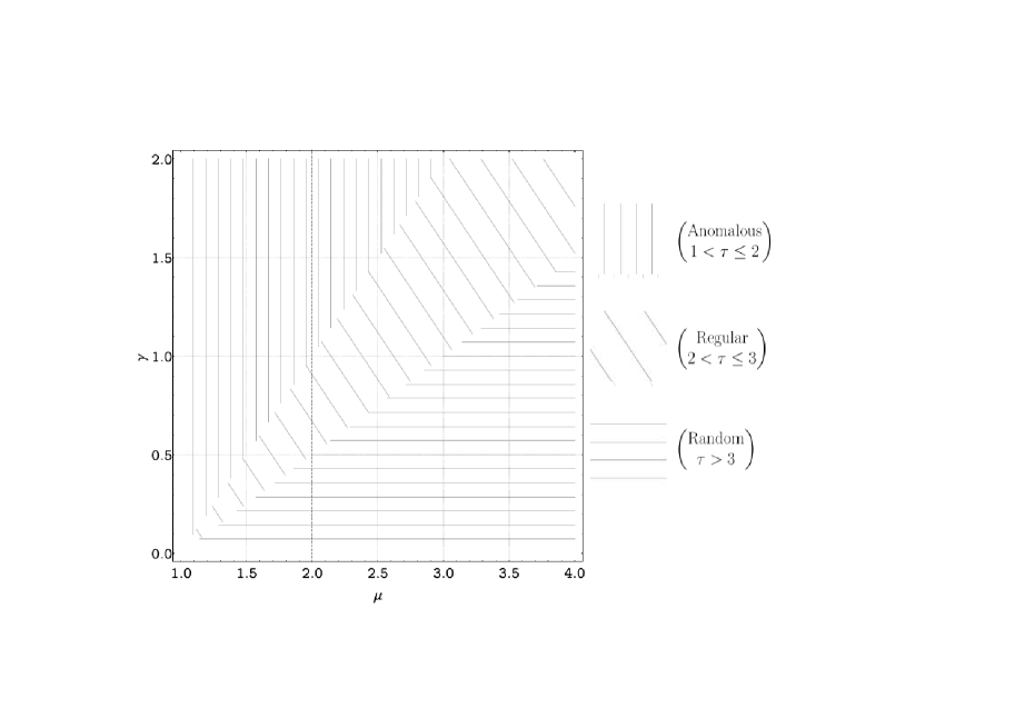
Refer to caption
Figure 11: Region of the space of parameters (ΞΌ,Ξ³)πœ‡π›Ύ(\mu,\gamma) where a scale free network exhibits three different behaviors in their degree distributions. Clockwise, on the top we have anomalous regime, then in the middle, regular networks, and on the bottom random-like networks. The vertical dashed black line represents the classical case in which ΞΌ=2πœ‡2\mu=2 ( Lux & Montagna). In this condition for the fitness density, regular scale free occurs for γ𝛾\gamma in (12,1]121(\frac{1}{2},1] . The anomalous regime occurs when Ξ³>1𝛾1\gamma>1. Eventually, random-like behavior occurs for γ∈(0,12]𝛾012\gamma\in(0,\frac{1}{2}]

This discussion can set a range for the out-degree and in-degree coefficients choosing correct values α𝛼\alpha and β𝛽\beta of the linking function to have a scale free behavior in the degree-distributions.

An important subcase of this network is for

Ξ³=Ξ±=Ξ²=0𝛾𝛼𝛽0\gamma=\alpha=\beta=0

for which

f​(xi,xj)=c​o​n​s​t=c𝑓subscriptπ‘₯𝑖subscriptπ‘₯π‘—π‘π‘œπ‘›π‘ π‘‘π‘f(x_{i},x_{j})=const=c

. Then from the eq.(5), using the power law distribution for the fitness function, we have:

ko​u​t​(x)N=subscriptπ‘˜π‘œπ‘’π‘‘π‘₯𝑁absent\displaystyle\frac{k_{out}(x)}{N}= ∫abf​(x,s)​ρ​(s)​𝑑ssuperscriptsubscriptπ‘Žπ‘π‘“π‘₯π‘ πœŒπ‘ differential-d𝑠\displaystyle\int_{a}^{b}f(x,s)\rho(s)ds (150)
=\displaystyle= cβ€‹βˆ«abC[a,b]​sβˆ’ΞΌβ€‹π‘‘s=c𝑐superscriptsubscriptπ‘Žπ‘subscriptπΆπ‘Žπ‘superscriptπ‘ πœ‡differential-d𝑠𝑐\displaystyle\,c\int_{a}^{b}C_{[a,b]}\,s^{-\mu}ds=c (151)

From which we have the same degree per node, that is the case of the random graph with average degree controlled by the number of links created in the preferential attachment procedure:

⟨k⟩=c​N=LN,delimited-βŸ¨βŸ©π‘˜π‘π‘πΏπ‘\langle k\rangle=cN=\frac{L}{N}, (152)

from which c=L/N2𝑐𝐿superscript𝑁2c=L/N^{2} which plays the role of probability in Erdos-Renyi network.

In this case non scale free behavior exists. A big difference between a random-like network and a scale-free one is also evident in the network layout as in fig.12, where the scale-free network shows a core-periphery structure.
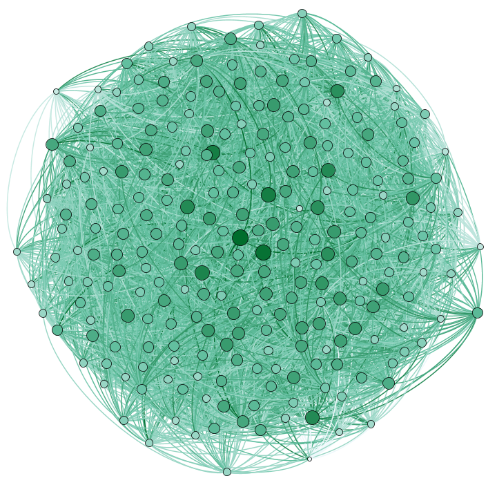
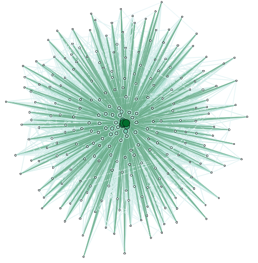
Refer to caption
(a) Structure of bank network in the regime of random graph
Refer to caption
(b) Scale free bank network in the regime of graph where it is evident the core-periphery attitude in such kind of networks.
Figure 12: Layout of random (a) and scale free (b) networks.

Bibliography

  • Barrat etΒ al., [2004] Barrat, A., Barthelemy, M., Pastor-Satorras, R., and Vespignani, A. (2004). The architecture of complex weighted networks. Proceedings of the National Academy of Sciences of the United States of America, 101(11):3747–3752.
  • Bedogne and Rodgers, [2006] Bedogne, C. and Rodgers, G. (2006). Complex growing networks with intrinsic vertex fitness. Physical Review E, 74(4):046115.
  • BogunΓ‘ and Pastor-Satorras, [2003] BogunΓ‘, M. and Pastor-Satorras, R. (2003). Class of correlated random networks with hidden variables. Physical Review E, 68(3):036112.
  • BogunΓ‘ etΒ al., [2004] BogunΓ‘, M., Pastor-Satorras, R., and Vespignani, A. (2004). Cut-offs and finite size effects in scale-free networks. The European Physical Journal B-Condensed Matter and Complex Systems, 38(2):205–209.
  • BogunΓ‘ and Serrano, [2005] BogunΓ‘, M. and Serrano, M. Á. (2005). Generalized percolation in random directed networks. Physical Review E, 72(1):016106.
  • Bornholdt and Schuster, [2003] Bornholdt, S. and Schuster, H.Β G., editors (2003). Handbook of Graphs and Networks: From the Genome to the Internet. John Wiley & Sons, Inc., New York, NY, USA.
  • Bottazzi, [2009] Bottazzi, G. (2009). On the pareto type iii distribution. Technical report, LEM Working Paper Series.
  • Bottazzi etΒ al., [2016] Bottazzi, G., DeΒ Sanctis, A., and Vanni, F. (2016). Non-performing loans, systemic risk and resilience in financial networks. Technical report, LEM Working Paper Series.
  • Caldarelli, [2007] Caldarelli, G. (2007). Scale-free networks: complex webs in nature and technology. OUP Catalogue.
  • Caldarelli etΒ al., [2002] Caldarelli, G., Capocci, A., DeΒ LosΒ Rios, P., and Munoz, M.Β A. (2002). Scale-free networks from varying vertex intrinsic fitness. Physical review letters, 89(25):258702.
  • Caldarelli and Chessa, [2016] Caldarelli, G. and Chessa, A. (2016). Data Science and Complex Networks: Real Case Studies with Python. Oxford University Press.
  • Catanzaro etΒ al., [2005] Catanzaro, M., BoguΓ±Γ‘, M., and Pastor-Satorras, R. (2005). Generation of uncorrelated random scale-free networks. Physical Review E, 71(2):027103.
  • Chaudhry and Zubair, [1994] Chaudhry, M.Β A. and Zubair, S.Β M. (1994). Generalized incomplete gamma functions with applications. Journal of Computational and Applied Mathematics, 55(1):99–123.
  • Dorogovtsev and Mendes, [2002] Dorogovtsev, S.Β N. and Mendes, J. (2002). Accelerated growth of networks. arXiv preprint cond-mat/0204102.
  • Dorogovtsev and Mendes, [2013] Dorogovtsev, S.Β N. and Mendes, J. (2013). Evolution of Networks: From Biological Nets to the Internet and WWW. Oxford University Press.
  • Dorogovtsev and Mendes, [2001] Dorogovtsev, S.Β N. and Mendes, J. F.Β F. (2001). Effect of the accelerating growth of communications networks on their structure. Phys. Rev. E, 63:025101.
  • Foss etΒ al., [2013] Foss, S., Korshunov, D., and Zachary, S. (2013). Heavy-tailed and long-tailed distributions. In An Introduction to Heavy-Tailed and Subexponential Distributions, pages 7–42. Springer.
  • Gai and Kapadia, [2010] Gai, P. and Kapadia, S. (2010). Contagion in financial networks. Proceedings of the Royal Society A: Mathematical, Physical and Engineering Science, page rspa20090410.
  • Hoppe and Rodgers, [2015] Hoppe, K. and Rodgers, G. (2015). A microscopic study of the fitness-dependent topology of the world trade network. Physica A: Statistical Mechanics and its Applications, 419:64–74.
  • Latora etΒ al., [2017] Latora, V., Nicosia, V., and Russo, G. (2017). Complex networks: principles, methods and applications. Cambridge University Press.
  • Leskovec etΒ al., [2005] Leskovec, J., Kleinberg, J., and Faloutsos, C. (2005). Graphs over time: densification laws, shrinking diameters and possible explanations. In Proceedings of the eleventh ACM SIGKDD international conference on Knowledge discovery in data mining, pages 177–187. ACM.
  • Mastrandrea etΒ al., [2014] Mastrandrea, R., Squartini, T., Fagiolo, G., and Garlaschelli, D. (2014). Enhanced reconstruction of weighted networks from strengths and degrees. New Journal of Physics, 16(4):043022.
  • Montagna and Lux, [2013] Montagna, M. and Lux, T. (2013). Hubs and resilience: towards more realistic models of the interbank markets. Technical report, Kiel Working Paper.
  • Restrepo etΒ al., [2007] Restrepo, J.Β G., Ott, E., and Hunt, B.Β R. (2007). Approximating the largest eigenvalue of network adjacency matrices. Physical Review E, 76(5):056119.
  • Salsa, [2016] Salsa, S. (2016). Partial differential equations in action: from modelling to theory, volumeΒ 99. Springer.
  • [26] Serrano, M., BoguΓ±Γ‘, M., Pastor-Satorras, R., and Vespignani, A. (2007a). Large scale structure and dynamics of complex networks: from information technology to finance and natural sciences. Correlations in complex networks, journal, pages 35–66.
  • [27] Serrano, M.Β A., BoguΓ±Γ‘, M., Pastor-Satorras, R., and Vespignani, A. (2007b). Correlations in complex networks. Large scale structure and dynamics of complex networks: From information technology to finance and natural sciences, pages 35–66.
  • Servedio etΒ al., [2004] Servedio, V.Β D., Caldarelli, G., and Butta, P. (2004). Vertex intrinsic fitness: How to produce arbitrary scale-free networks. Physical Review E, 70(5):056126.
  • Squartini and Garlaschelli, [2011] Squartini, T. and Garlaschelli, D. (2011). Analytical maximum-likelihood method to detect patterns in real networks. New Journal of Physics, 13(8):083001.
  • Vespignani and Caldarelli, [2007] Vespignani, A. and Caldarelli, G. (2007). Large scale structure and dynamics of complex networks: from information technology to finance and natural science, volumeΒ 2. World Scientific.
  • Xu etΒ al., [2010] Xu, X.-J., Zhang, L.-M., and Zhang, L.-J. (2010). Mutual selection in network evolution: the role of the intrinsic fitness. International Journal of Modern Physics C, 21(01):129–135.