Ringing Non-Gaussianity from inflation with a step in the second derivative of the potential

Abstract

Inflationary model driven by a scalar field whose potential has a step in the second derivative with respect to the field is considered. For the best fit potential parameter values, the 3-point function and the non-Gaussianity associated with the featured model is calculated. We study the shape and scale dependence of the 3-point function. The distinctive feature of this model is its characteristic ringing behaviour of $f_{NL}$. We can see that the oscillations in $f_{NL}$ in this model last for a much longer range of k values, as compared to the previously studied models. In that sense, this model is potentially distinguishable from models with other features in the potential.

1 Introduction

In standard slow-roll inflation the deviation from Gaussian distribution of the primordial perturbations [1, 2, 3] is predicted to be small. It is of the order of the slow-roll parameters [4, 5, 6, 7]. This result does not hold if the the inflaton undergoes a period of slow-roll violation during its evolution [8, 9, 10, 11], as can happen if the inflaton potential has some localized feature [12]. The resulting non-Gaussianity [13] then becomes shape and scale dependent and modes that exit Hubble scale around the time the field cross the feature can pick up large non-Gaussianities. An inflationary model where the inflaton potential has a feature in its second derivative with respect to the inflaton has been proposed in [14]. In that paper, the authors showed that the power spectrum picks of small oscillations superimposed on a flat spectrum and the spectral index can experience a jump around the feature. This scenario helps to explain the local running in the spectral index observed in the WMAP and Planck data [15, 16, 17]. In the present work, we are interested in studying the non-Gaussianity predicted by this model. The analysis of the running of non-Gaussianity using Planck data is given in [18], in the context of some well defined inflationary models. Inflationary models that predicts a mildly scale dependent bispectrum, termed as the running of the bispectrum [19, 20, 21] is discussed there. In the present work, we compute the 3-point function of the curvature perturbation and study the shape and scale dependence of the 3-point function. The paper is organized as follows: in section 2 we describe our model and give the background evolution and the resulting power spectrum of curvature perturbations. In section 3 we compute the three-point function and the non-Gaussianity from the model and then conclude by summarizing our results in section 4.

2 The model with a step in the second derivative of the potential

In [14] we showed that the well-known model with a Higgs-like potential which is used in the hybrid inflationary scenario too,

$$V(\psi,\phi)=\frac{1}{4\lambda}\left(M^{2}-\lambda\psi^{2}\right)^{2}+\frac{1}{2}m^{2}\phi^{2}+\frac{g^{2}}{2}\phi^{2}\psi^{2}~{},$$ (1)

could successfully give rise to a step in the primordial spectral index. At $\phi_{c}=M/g$ the curvature of $V(\psi,\phi)$ along the $\psi$ direction vanishes so that $m_{\psi}^{2}>0$ for $\phi>\phi_{c}$ while $m_{\psi}^{2}<0$ for $\phi<\phi_{c}$. This implies that for large values of the inflaton $\phi$ the auxiliary field $\psi$ rolls towards $\psi=0$. However, once the value of $\phi$ falls below $\phi_{c}$ the $\psi=0$ configuration is destabilized resulting in a rapid cascade (mini-waterfall) which takes $\psi$ from $\psi=0$ to its minimum value. This potential has four parameters, namely, M, m, g and $\lambda$. The model confrontation with WMAP–7 data has been done in [22] and the best fit values of potential parameters were obtained with N = 40 and N = 60, where N represents the number of e-folds after the phase transition. Table below gives the potential paramters best fit with the Bicep-Keck-Planck likelihoods (combined BICEP2 and Keck Array October 2018 data in combination with the 2018 Planck data)[23, 24, 25].

Parameter	Values for N=60	Values for N=40
$M/m_{pl}$	7.43$\times$ $10^{-4}$	8.22 $\times$ $10^{-4}$
$m/m_{pl}$	4.6$\times$ $10^{-7}$	6.9$\times$ $10^{-7}$
$g$	2.77 $\times$ $10^{-4}$	3.75 $\times$ $10^{-4}$
$\lambda$	0.1	0.1

Table 1: Best fit values of Potential Parameters

2.1 Background Evolution

With this potential, by initiating evolution with initial field value $\phi_{i}>\phi_{c}$, the coupled system of equations of the background inflaton and scale factor of expansion of spacetime exhibits inflation with the inflaton rolling the potential, till inflation ends and $\phi$ finally oscillating about the potential minimum. The slow-roll conditions $\epsilon$, $\eta<1$, where $\epsilon$, $\eta$ are given by

$$\epsilon\equiv 3\frac{\dot{\phi}^{2}/2}{\dot{\phi}^{2}/2+V},\hskip 56.9055pt\eta\equiv-3\frac{\ddot{\phi}}{3H\dot{\phi}}$$

are satisfied throughout the inflationary period. However, $\eta$ has a discontinuity at $\phi=\phi_{c}$ since it is proportional to $V^{\prime\prime}$. We explore the consequences of this discontinuity in the behaviour of the two-point and three-point functions of the perturbations of the dynamical variables.

2.2 Two-point function and power spectrum of scalar perturbations

The Fourier modes of the curvature perturbation satisfies the equation

$${\cal R}^{\prime\prime}_{k}+2\frac{z^{\prime}}{z}{\cal R}^{\prime}_{k}+k^{2}{\cal R}_{k}=0$$ (2)

where the prime denotes derivative with respect to conformal time and the quantity $z$ is given by

$$z\equiv\frac{a}{H}\sqrt{\rho+p}=\frac{a\dot{\phi}}{H}$$ (3)

${\cal R}$ is related to the Mukhanov-Sasaki variable u as ${\cal R}=u/z$. The scalar power spectrum is then defined as

$${\cal P}_{s}(k)=\frac{k^{3}}{2\pi^{2}}|{\cal R}_{k}|^{2}$$ (4)

with the amplitude of the curvature perturbation ${\cal R}_{k}$ evaluated, in general, at the end of inflation.

Under slow-roll, the power spectrum is approximately given by

$${\cal P}_{s}(k)\simeq\frac{1}{2\epsilon}\frac{H^{2}}{2\pi}\left(\frac{k}{aH}\right)^{2}$$ (5)

with $n_{s}$ given in terms of slow-roll parameters as

$$n_{s}\simeq 1-2\epsilon-\eta$$ (6)

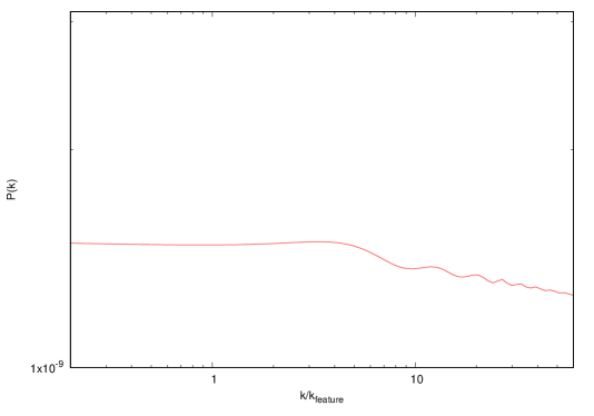
For the potential given by Eq.(1), one can immediately notice that $n_{s}$ will have discontinuity due to its dependence on $\eta$. This will result in the power spectrum having a jump in its slope at a scale set by $\phi_{c}$. The full analytic expression for the power spectrum has small oscillations superimposed around the scale of change of slope, as shown in [14]. Figure 1 shows the quasi flat $\mathcal{P}_{k}$ for this mini waterfall hybrid model.

Figure 1: Primordial spectrum for a model with step in the second derivative of the potential

3 Three-point function and non-Gaussianity from the model

Our approach is based on the numerical evaluation of both the perturbation equations and the integrals which contribute to the 3-point function as described by Chen etal in [8, 9]. To compute the 3-point correlation function, one can substitute the mode solutions $u_{k}$ into equation (3.17) of [8], and integrate the mode functions from $\tau_{0}$ through to the end of inflation. This integral can be done semi-analytically for simple models, provided the slow-roll parameters are small and relatively constant. For standard single field slow-roll inflation, the terms of order $\epsilon^{2}$ in the above mentioned equation are the dominant contributors to the 3-point function and the other terms of order $\epsilon\eta^{\prime}$ and $\epsilon^{3}$ were neglected in Refs. [4, 5, 6]. In the presence of a step in the potential, the $\epsilon\eta^{\prime}$ term becomes large and dominant [8, 9]. The step in the second order derivative of the potential will make the $\epsilon\eta^{\prime}$ term much higher compared to $\epsilon^{2}$ term and hence leads to a modification of the standard slow-roll results. Thus the term of our particular interest is the $\epsilon\eta^{\prime}$ term

$$I_{\epsilon\eta^{\prime}}\propto i\left(\prod_{i}u_{i}(\tau_{end})\right)\int_{\infty}^{\tau_{end}}d\tau a^{2}\epsilon\eta^{\prime}\left(u_{1}^{*}(\tau)u_{2}^{*}(\tau)\frac{d}{d\tau}u_{3}^{*}(\tau)+\hskip 5.69046pttwo~{}perm\right)\times$$

$$\hskip 85.35826pt\left(2\pi\right)^{3}\delta^{3}\left(\sum_{i}\textbf{k}_{i}\right)+c.c$$ (7)

where the “two perm” stands for two other terms that are symmetric under permutations of the indices 1, 2 and 3, where 1, 2, 3 are shorthand for $k_{1}$, $k_{2}$ and $k_{3}$. For our step model, $\epsilon\eta^{\prime}$ can be written as,

$$\epsilon\eta^{\prime}=6aH\left(2\epsilon^{2}-\frac{\epsilon\eta}{2}+\frac{5}{6}{\epsilon^{2}\eta}-\frac{2}{3}\epsilon^{3}-\frac{\epsilon\eta^{2}}{12}-\epsilon\frac{V_{\phi\phi}}{3H^{2}}\right)$$ (8)

In order to integrate Eq. (7) numerically, we follow the procedure detailed in [9]. For the present model with a step in the second deriavative of the potential,

$$\nu_{k}(\tau_{0})=\frac{\sqrt{\pi\tau}}{2}H_{\mu_{1}}^{(2)}(k\tau_{0})~{},$$ (9)

where $H_{\mu_{1}}^{(2)}(k\tau_{0})$ is the Hankel function and ${\mu_{1}}=\frac{3}{2}-\frac{V^{\prime\prime}_{-}}{3H_{0}^{2}}+3\epsilon_{0}$, where $V^{\prime\prime}_{-}\equiv\left(\frac{d^{2}V}{d\varphi^{2}}\right)_{\rm before\hskip 2.84544ptphase\hskip 2.84544pttransition}$.

Every 3-point correlation function has two main attributes: shape and scale. Following [8, 9] we define the parameter, $\cal G$ to describe non-Gaussianities with both shape and scale dependence:

$$\frac{{\cal G}(k_{1},k_{2},k_{3})}{k_{1}k_{2}k_{3}}\equiv\frac{1}{\delta^{3}(\textbf{k}_{1}+\textbf{k}_{2}+\textbf{k}_{3})}\frac{(k_{1}k_{2}k_{3})^{2}}{P_{k}^{2}(2\pi)^{7}}\langle\zeta(\textbf{k}_{1})\zeta(\textbf{k}_{2})\zeta(\textbf{k}_{3})\rangle$$ (10)

In the absence of the sharp feature, Eq. (10) reduces to the local form with

$${\cal G}=(3/10)f_{NL}^{local}\sum k_{i}^{3}$$ (11)

Using Eqs. (10) and (11), we can calculate the non-Gaussianity parameter, $f_{\rm NL}^{\rm local}$, for our model.

$$\langle\zeta(\textbf{k}_{1})\zeta(\textbf{k}_{2})\zeta(\textbf{k}_{3})=(2\pi)^{7}\delta^{3}(\textbf{k}_{1}+\textbf{k}_{2}+\textbf{k}_{3})\left(-\frac{3}{10}f_{NL}\mathcal{P}_{k}^{2}\right)\frac{\Sigma_{i}k_{i}^{3}}{\Pi_{i}k_{i}^{3}}$$ (12)

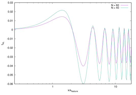
Since this model has already been used to improve the fit between LCDM cosmology and the observed power spectrum, we can take the best fit potential parameter values and compute the resulting 3-point function. Figure 2 gives the $f_{NL}^{equil}$ for our model, for the equilateral configuration ($k_{1}=k_{2}=k_{3}$). Purple line is for N = 60 and green for N = 40. The numerical value is not much larger than those in standard single filed, slow-roll inflation. The distinctive feature of this non-Gaussianity is its characteristic ringing behaviour of $f_{NL}$.

Figure 2: $f_{NL}^{equil}$ for the equilateral case. x axis is $k/k_{feature}$

We can see that the oscillations in $f_{NL}$ in this model last for a much longer range of k values, as compared to the previously studied models [8, 9]. In that sense, this model is potentially distinguishable from models with other features in the potential.

4 Conclusion

The single filed, slow-roll models of inflation generically yields a negligible primordial non-Gaussianity, which is not even observable. Thus the bispectrum analysis of CMB data can be considered as a promising candidate to discriminate between the degenerate inflationary models. In the present work, we considered a variant of hybrid inflation where the potential has a discontinuity in its second derivative with respect to field. This describes a fast second order phase transition during inflation that occurs in some other scalar field weakly coupled to the inflaton. The 3-point correlation function is numerically integrated for this anomalous inflationary model where slow-roll is violated for a brief moment. The transient violation of the slow-roll leads to an oscillating and scale dependent 3-point function. For the typical potential parameter values, non-Gaussianity associated with the featured potential model is found to be oscillating.

The distinctive feature of this non-Gaussinaity is its characteristic ringing behaviour; $f_{NL}$ oscillates between a maximum and minimum value. The oscillations in $f_{NL}$ in this model last for a much longer range of k values, as compared to the previously studied models. In that sense, this model is potentially distinguishable from models with other features in the potential.

References

- [1] A. A. Starobinsky, Phys, Lett. B 117, 175 (1982)
- [2] V. F. Mukhanov, H. A. Feldman and R. H. Brandenberger, “Theory of cosmological perturbations Part 1. Classical perturbations. Part 2. Quantum theory of perturbations. Part 3. Extensions,” Phys. Rept. 215, 203 (1992).
- [3] Lyth D. H, Malik K. A and Sasaki M, JCAP 0505, 004 (2005)[arXiv:astro-ph/0411220].
- [4] J. M. Maldacena, JHEP 0305, 013 (2003) [arXiv:astro-ph/0210603].
- [5] D. Seery and J. E. Lidsey, JCAP 0506, 003 (2005) [arXiv:astro-ph/0503692].
- [6] X. Chen, M. X. Huang, S. Kachru and G. Shiu, JCAP 0701, 002 (2007) [arXiv:hep-th/0605045].
- [7] G. Cabass, E. Pajer and F. Schmidt, JCAP 1701 01, 003 (2017)
- [8] X. Chen, Easther and Lim, JCAP 0706, 023 (2007) [astro-ph//0611645]
- [9] X. Chen, Easther and Lim, JCAP 0804, 010 (2008) [astro-ph//0801645]
- [10] A. A. Abolhasani, H. Firouzjahi, S.Khosravi, M. Sasaki, JCAP 1211, 012 (2012) [arXiv:1204.3722].
- [11] D. K. Hazra, L. Sriramkumar, J. Martin JCAP 05, 026 (2013) [arXiv:1201.0926]
- [12] P. Adshead, C. Dvorkin, W. Hu, E. A. Lim, Phys. Rev. D 85, 023531 (2012), [arXiv:1110.3050]
- [13] P. D. Meerburg et al, Astro2020 Science White Paper : Primordial Non-Gaussinaity (2019), [arXiv:1903.04409] and the references therein.
- [14] Minu Joy, V. Sahni and A. A. Starobinsky, Phys. Rev. D 77, 023514 (2008) [arXiv:0711.1585].
- [15] E. Komatsu, J. Dunkley, M.R. Nolta et al., Astrophys.J.Suppl. 180 (2009) [arXiv:0803.0547]; J. Dunkley, E. Komatsu, M.R. Nolta et al., Astrophys.J.Suppl. 180 (2009) [arXiv:0803.0586].
- [16] Planck collaboration, Planck 2015 results. XX.Constraints on Inflation, A A, 594, A20 (2016), arXiv:1502.02114
- [17] Planck collaboration, Planck 2018 results. X.Constraints on Inflation, Y. Akrami et al A A, 641, A10 (2020) (2018), [arXiv:1807.06211].
- [18] Planck collaboration, Planck 2018 results. IX. Constraints on Primordial non-Gaussinaity, Y. Akrami et al, A A, 641 A9 (2020) [arXiv:1905.05697].
- [19] X. Chen, Phys. Rev. D 72, 123518 (2005), [arXiv:astro-ph/0507053]
- [20] C. Byrnes et al, JCAP 10, 004 (2010) [arXiv:1007.4277]; C. Byrnes et al, JCAP 2, 0034 (2010) [arXiv:0911.2780].
- [21] S. Shandera et al, JCAP 3, 017 (2011) [arXiv:1010.3722].
- [22] Minu Joy, A. Shafieloo, V. Sahni and A. A. Starobinsky, JCAP 0906, 028 (2009) [arXiv:0807.3334].
- [23] CosmoMC -
- [24] BICEP2 Keck and Planck Collaborations, P. A. R. Ade et al, Phys. Rev. Lett. 114, 101301 (2015)
- [25] BICEP2 Keck Array X, P. A. R. Ade et al, Phys. Rev. Lett. 121, 221301 (2018)