Gradient Boosted Binary Histogram Ensemble
for Large-scale Regression
Abstract
In this paper, we propose a gradient boosting algorithm for large-scale regression problems called Gradient Boosted Binary Histogram Ensemble (GBBHE) based on binary histogram partition and ensemble learning. From the theoretical perspective, by assuming the Hölder continuity of the target function, we establish the statistical convergence rate of GBBHE in the space and , where a lower bound of the convergence rate for the base learner demonstrates the advantage of boosting. Moreover, in the space , we prove that the number of iterations to achieve the fast convergence rate can be reduced by using ensemble regressor as the base learner, which improves the computational efficiency. In the experiments, compared with other state-of-the-art algorithms such as gradient boosted regression tree (GBRT), Breiman’s forest, and kernel-based methods, our GBBHE algorithm shows promising performance with less running time on large-scale datasets.
Keywords: Large-scale regression, binary histogram partition, random rotation, gradient boosting, ensemble learning, regularized empirical risk minimization, learning theory
1 Introduction
Over the past two decades, boosting has become one of the most successful algorithms in the machine learning community (Bühlmann and Yu, 2003). After the idea of iterative utilization of weak learners from a certain function space to generate a strong one, which is called boosting, first came out in Schapire (1990); Freund (1995), it gains a lot of attention, and a wealth of literature has applied it to a large number of datasets. During this period, many boosting algorithms with impressive performance have been proposed. The first boosting algorithm dates back to the Adaboost for classification by Schapire and Freund (1995); Freund and Schapire (1997). Another important boosting algorithm for regression called Gradient Boosted Regression Tree (GBRT) was proposed by Friedman (2001). GBRT takes advantage of tree-based learners to capture complex data structures.
In addition to the great success of these boosting algorithms, a lot of attempts have been made to establish their theoretical foundations. For example, from the perspective of statistical analysis, Bühlmann and Yu (2003) derived an exponential bias-variance trade-off for linear regression to illustrate the almost resistance to overfitting for -boosting in a fixed design setting. Moreover, Park et al. (2009) and Lin et al. (2019) established the theoretical analysis of boosting methods using Nadaraya-Watson kernel estimates and kernel ridge regression estimates as base learners, respectively. However, these methods are of little value in practice since they fail to capture the complex data dependencies in applications. In the prior work of this paper (Cai et al., 2020), we proposed a boosting algorithm for regression problems called boosted histogram transform for regression (BHTR) with sound theoretical guarantees and satisfactory empirical performance. However, since it utilizes the ordinary histogram transforms as base learners, the number of partition cells grows exponentially with the dimension, and thus is hard to adapt to high-dimensional data.
Moreover, despite the success in achieving desirable performance, boosting procedures can encounter heavy computational costs in the computations of the features and the selection of the weak learner, both of which depend on the number of features and the number of training examples. Therefore, boosting algorithms cannot be directly applied to large-scale high-dimensional data. Efforts have been made to further enhance the efficiency of boosting algorithms in large-scale scenarios. For example, Dubout and Fleuret (2014) utilized an adaptive sampling approach to sample features at every boosting step, so as to reduce computational cost. Other works focus on enhancing the efficiency of boosting through engineering optimizations: Chen and Guestrin (2016) came up with the eXtreme Gradient Boosting (XGBoost), which achieves excellent experimental performance. Ke et al. (2017) speeds up the training process of conventional GBRT by up to over 20 times. More recently, Biau et al. (2019) incorporates the Nesterov’s accelerated gradient descent technique (Nesterov, 1983) to accelerate GBRT. Unfortunately, none of the above-mentioned boosting works for large-scale regression presents a satisfactory statistical theoretical guarantee.
Under such background, this paper aims to establish a new boosting algorithm for large-scale and high-dimensional regression, which is not only with satisfactory performance but also with solid theoretical foundations. To be specific, motivated by the random rotation ensemble algorithms (López-Rubio, 2013; Blaser and Fryzlewicz, 2016) and binary histogram partition (Biau, 2012), we propose gradient boosted binary histogram ensemble (GBBHE) for regression, where we for the first time combine two ensemble methods, i.e. gradient boosting and base learner aggregation, to enhance effectiveness and computational efficiency. First of all, we apply a random rotation to the input space and apply the binary histogram partition, with the help of which we obtain piecewise constant base learners. Then at each iteration, we generate several independent base learners and ensemble them by taking the arithmetic average, where we call the ensemble estimator rotated binary histogram ensembles. The iterative process to fit residuals is started with the help of a sequence of rotated binary histogram ensembles by a natural adaption of gradient descent boosting algorithm.
It is worth mentioning that GBBHE enjoys four advantages. Firstly, our obtained regression function can be globally smooth thanks to the diversity of different base learners resulting from the randomness of both random rotations and binary histogram partitions. Secondly, under binary histogram partitions, all cells are split to the same depth, which ensures the fast convergence of our algorithm. Thirdly, compared with ordinary histograms, our binary histogram partition split at the midpoint of only one selected side at each iteration, so the cells will not be too small and thus it applies better to high dimensional data. Finally, GBBHE applies well to the large-scale scenarios since the more accurate base ensembles, enjoying high computational efficiency with the help of parallel computing, can effectively reduce the number of iterations in boosting.
As follows are the contributions of this paper.
(i) Aiming at solving the large-scale regression problem, we propose a novel boosting algorithm named Gradient Boosted Binary Histogram ensemble (GBBHE), where the binary histogram regressors are used as base learners and the ensemble method performed on base learners helps improve its computational efficiency by reducing the number of boosting iterations. We claim that the binary histogram partition is adapted well to high-dimensional data, compared with ordinary histogram partitions.
(ii) From the theoretical perspective, we first of all investigate a special case of GBBHE, that is, GBBHE without ensemble (abbreviated as GBBH), where the number of base learners in an ensemble is set to be . Under the assumption that the target function resides in and , respectively, by decomposing the error term into approximation error and sample error, we establish the fast convergence rates of GBBH in the space . Moreover, for the subspace consisting of smoother functions, we are able to show that GBBH can attain the asymptotical convergence rate whereas the lower bound of the convergence rates for its base learner binary histogram is merely of the order . As a result, we succeed to prove that the boosted regressor GBBH can achieve faster convergence rates than the base learner in the subspace when , which confirms the benefits of the proposed boosting procedure.
(iii) We further prove that GBBHE has the same convergence rates as that of GBBH in both and . However, compared with the results for GBBH, where the number of iterations is required to be of the order to achieve the convergence rate, for GBBHE, we only require that is of the same order , where denotes the number of ensembles at each iteration. In other words, we can reduce the number of iterations by enlarging the number of base learners for ensemble . It is well known that boosting algorithms with a large number of iterations can be quite time-consuming, since acceleration techniques such as parallel computing are not directly available. Therefore, by combining ensemble methods, which enjoy high computational efficiency with the help of parallel computing, we successfully save the running time of GBBHE by reducing the number of iterations .
(iv) In the experiments, several numerical experiments are designed to study the parameters including the depth of the binary histogram transform , the number of iterations of boosting , the number of binary histograms in each iteration , and learning rate . And we empirically verify the theoretical results that ensemble methods can reduce the number of iterations to achieve the fast convergence rate. Moreover, we compare our GBBHE with state-of-the-art large-scale regressors including GBRT, Breiman’s forest, and LiquidSVM on both moderate-sized and large-scale real datasets. It turns out that our GBBHE shows comparable or even better performance than the compared methods, while enjoys higher computational efficiency with less running time required.
This paper is organized as follows. In Section 2, we introduce the methodology of this paper, where we construct our main algorithm GBBHE. Then in Section 3, we present the theoretical results built for GBBHE and its special case GBBH in Hölder space consisting of -Hölder continuous functions. We conduct numerical experiments including parameter analysis and real data comparisons with other state-of-the-art large-scale regression algorithms in Section 4. Finally, we present our comments and discussions in Section 5. We put the error analysis for Section 3 in Section 6 and the related proofs in Section 7.
2 Methodology
In this section, we build the main algorithm Gradient Boosted Binary Histogram Ensemble (GBBHE) for regression. We first introduce some notations in Section 2.1 and show the basics of least square regression in Section 2.2. Then in Section 2.3, we introduce the (rotated) binary histogram, which is an essential part in establishing the main algorithms. In Section 2.4, we show a special case of GBBHE where the number of ensembles equals to , called GBBH. Finally, in Section 2.5, we present the main algorithm of GBBHE.
2.1 Notations
Regression is to predict the value of an unobserved output variable based on the observed input variable , based on a dataset consisting of i.i.d. observations drawn from an unknown probability measure on . Throughout this paper, we assume that and are compact and non-empty.
For any fixed , we denote as the centered hyper-cube of with size , that is, . Recall that for , the -norm of is defined by , and the -norm is defined by .
In the sequel, the notation means that there exists some positive constant , such that and , for all . Similarly, the notation denotes that there exists some positive constant , such that and denotes that there exists some positive constant , such that . For any , let denote the largest integer less than or equal to . Moreover, the following multi-index notations are used frequently. For any vector , we write , , , , and .
2.2 Least Square Regression
It is legitimate to consider the least square loss defined by for our target of regression. Then, for a measurable decision function , the risk is defined by and the empirical risk is defined by . The Bayes risk, which is the smallest possible risk with respect to and , is given by .
In what follows, it is sufficient to consider predictors with values in . To this end, we introduce the concept of clipping for the decision function, see also Definition 2.22 in Steinwart and Christmann (2008). Let be the clipped value of at defined by if , if , and if . Then, a loss is called clippable at if, for all , there holds . According to Example 2.26 in Steinwart and Christmann (2008), the least square loss is clippable at with the risk reduced after clipping, i.e., . Therefore, in the following, we only consider the clipped version of the decision function as well as the risk .
2.3 Binary Histogram for Regression
In the following, we use the tilde notation to distinguish between the transformed space and the original input space.
2.3.1 Random Rotation
To give a clear description of one possible construction procedure of rotated random histograms, we start with the random rotation matrix , which is a real-valued orthogonal square matrix with unit determinant, that is
| (1) |
Then we define the rotation transformation by
| (2) |
In the following we will assume that each individual histogram is constructed in the transformed space .
Here we describe a practical method for the construction of the random rotation transformations we are confined to in this study. Starting with a square matrix , consisting of independent univariate standard normal random variates, a Householder decomposition is applied to obtain a factorization of the form , with orthogonal matrix and upper triangular matrix with positive diagonal elements. The resulting matrix is orthogonal by construction and can be shown to be uniformly distributed. Unfortunately, if does not feature a positive determinant then it is not a proper rotation matrix according to definition (1). In this case, we can change the sign of the first column of to construct a new rotation matrix that satisfies the condition (1).
2.3.2 Binary Histogram Partition
It is well known that the classical histogram partition is an effective algorithm by grouping samples into the bins with the same shape. However, ordinary histogram partition is plagued by the curse of dimensionality. That is, the number of bins grows exponentially with the dimension , in which case many bins will contain few or even no samples, leading to unacceptable and unnecessary computational costs. Therefore, we propose the binary partitioning technique to build the high-dimensional histogram, namely binary histogram.
To be specific, Let be the rectangular cell in the transformed space and be a deterministic parameter, fixed beforehand by the user, and possibly depending on . In the first step, we choose one of the coordinates with the -th feature having a probability of being selected, and then split into two rectangular cells along the midpoint of the chosen side. In other words, there exist such that , where and . In this way, we get a partition with two rectangular cells. Moreover, we denotes as the collection of partitions with two rectangular cells. Note that the total number of possible partitions after the first step is equal to the dimension . Suppose after steps of the recursion, we have obtained a partition of with rectangular cells. In the -th step, further partitioning of the region is defined as follows:
-
(i)
For each rectangular cell , , a coordinate of , namely is selected, with the -th feature having a probability to be chosen, that is,
(3) -
(ii)
For each rectangular cell , , once the coordinate is selected, the split is at the midpoint of the chosen side. As a result, each rectangular cell is divided into two new ones, namely and . We denote the set of all these cells by .
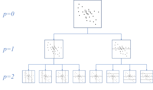
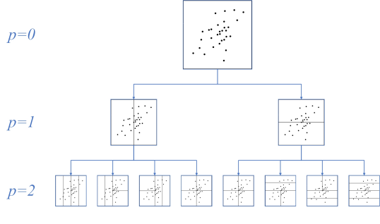
Such a partition obtained by recursive steps is called a binary histogram partition of with depth in the transformed space, and we say
| (4) |
an rotated binary histogram with depth in the input space , where for the set . The complete process is presented in Algorithm 1 and an illustration is shown in Figure 1.
For any , the histogram bin containing in the input space is
| (5) |
and we further denote all the bins as with the repetitive bin counted only once, and as the index set. In other words, the set forms a partition of .
2.3.3 Binary Histogram Regressor
We consider the following function set defined by
| (6) |
In order to constrain the complexity of , we penalize on the depth of the partition . Then the Binary Histogram with rotation can be produced by the regularized empirical risk minimization (RERM) over , i.e.
| (7) |
where . It is clear to see that the penalty on the depth of the partition helps to control the bin width of the rectangular cells.
2.4 Gradient Boosted Binary Histogram (GBBH) for Regression
Boosting is the task of converting inaccurate weak learners into a single accurate predictor. To be specific, we define a restricted family of functions be a set of base learners and a general boosting algorithm is combining a sequence of functions from to minimize a certain empirical loss. Then the final predictor can be represented as
where , , are weights and , . From a functional gradient descent viewpoint in statistics (Friedman, 2001), boosting is reformulated as a stage-wise optimization problem with different loss functions. In this scenario, gradient boosting requires computing the negative functional gradient as the response
and select a particular model from the allowable class of functions at each boosting iteration to update the predictor.
In this work, we mainly focus on the boosting algorithm equipped with (rotated) binary histogram regressors as base learners since they are weak predictors and enjoy computational efficiency in high dimensional spaces. Before we proceed, we need to introduce the function space that we are most interested in to establish our learning theory. Assume that is an i.i.d. sequence of random rotation matrix drawn from some probability measure and is an i.i.d. sequence of selected coordinate to split drawn from the probability measure given by (3). For , given rotation transformation and select coordinates , we define the function space , according to (6). Then for , we define the function space by
| (8) |
Moreover, for , we define
| (9) |
Then for any , by the Cauchy-Schwarz inequality, we immediately get
In fact, is a function space that consists of measurable and bounded functions.
As is mentioned above, boosting methods may be viewed as iterative methods for optimizing a convex empirical cost function. To simplify the theoretical analysis, following the approach of Blanchard et al. (2003), we ignore the dynamics of the optimization procedure and simply consider minimizers of an empirical cost function to establish the oracle inequalities, which leads to the following definition.
Definition 1
Let be the function space (8) and be the least square loss. Given , , we call a learning method that assigns to every a function such that
| (10) |
a gradient boosted binary histogram (GBBH) algorithm for regression with respect to , where is defined by
| (11) |
The regularization term defined in (11) consists of two components. The first term is motivated by the fact the early boosting methods such as Adaboost may overfit in the presence of label noise. It helps control the degree of overfitting by the -norm of the weights of the composite estimators and helps achieve the consistency and convergence results. The second term is added to control the bin width of the binary histogram, which has been discussed in subsection 2.3. In fact, it is equivalent to adding the -norm of the base learners , since piecewise constant functions are applied on the rectangular cells.
To conduct the theoretical analysis, we also need the infinite sample version of Definition 1. To this end, we fix a distribution on and let the function space be as in (8). Then every satisfying
is called an infinite sample version of GBBH with respect to and . Moreover, the approximation error function is defined by
| (12) |
With all these preparations, we now present a general form of algorithm for GBBH in Algorithm 2. Indeed, the randomness of rotation matrix and binary histogram splitting rule provides an effective procedure for carrying out boosting. With the help of (rotated) binary histogram regressor, we repeat the least squares fitting of residuals. We mention that when the rotation matrix is determined as the identity matrix, we call the algorithm in Algorithm 2 GBBH without rotation. Moreover, we introduce the learning rate to dampen the move on the gradient descent update, which is related to the regularization through shrinkage.
Remark 2
In fact, the Gradient Boosting Algorithm 2 converges to the empirical risk minimizer of the mean squared error with respect to the function space defined by (8)
| (13) |
which is illustrated as below:
-
(i)
In the least-square regression setting, the goal of a gradient boosting algorithm with stages is to fit a function of the form to minimize (13).
-
(ii)
At stage , our algorithm should add some new estimator to improve some imperfect model to correct the errors of its predecessor. For regression problems, we observe that residuals are the negative gradients (with respect to ) of the squared error loss function . Then gradient boosting will fit from the hypothesis space defined as in (6) to the residuals .
-
(iii)
Algorithm 2 does so by starting with a model , and incrementally expands it in a greedy fashion. The main idea is to apply a (functional gradient) descent step to this minimization problem to solve the computationally infeasible optimization problem in general.
-
(iv)
The regularization of gradient boosting methods is realized by shrinkage which consists of modifying the update rule with learning rate as shown in Algorithm 2 to improve the generalization ability of the model.
In summary, in accordance with the empirical risk minimization principle, gradient boosting algorithm tries to find an approximation that minimizes the average value of the loss function on the training set, i.e., minimizes the empirical risk with respect to the space defined by (8).
2.5 Gradient Boosted Binary Histogram Ensemble (GBBHE) for Large-scale Regression
For large-scale regression problems, however, GBBH may be of low computational efficiency since it requires a large number of boosting iterations in practical applications. As a result, it is important to find some ways to speed up the applications of GBBH. An intuitive idea is to increase the accuracy of the base learner and thus reduce the number of iterations. To be specific, we proposed a modified boosting algorithm using the ensemble of (rotated) binary histogram regressors as base learners. Recall that in Algorithm 2, at -th round of boosting iteration, gradient boosting requires computing the negative functional gradient as the response
| (14) |
and select a particular model to fit residuals to update the current predictor .
Before we proceed, we denote the number of boosting iterations as and the number of learners for ensemble at each boosting iteration as . Moreover, we assume that is an i.i.d. sequence of random rotation matrix drawn from some probability measure and is an i.i.d. sequence of selected coordinate to split drawn from the probability measure given by (3). For and , given the rotation transformation and select coordinates , we define the function space according to (6). In the scenario of gradient boosted binary histogram ensemble for large-scale regression, at -th round of boosting iteration, let be the training data with , defined by (14). For , we write
| (15) |
Then the ensemble of the (rotated) binary histogram regressor at -th round of boosting is defined by
It is clear to see that belongs to the function space given by
| (16) |
Then we define the function space by
| (17) |
Moreover, for , we define
which is similar as (9) where (rotated) binary histogram regressors are used as base learners.
To simplify the theoretical analysis, by similar arguments in Section 2.4, we ignore the dynamics of the optimization procedure and simply consider minimizers of an empirical cost function to establish the oracle inequalities for GBBHE, which leads to the following definition.
Definition 3
Let be the function space (17) and be the least square loss. Given , , we call a learning method that assigns to every a function such that
| (18) |
a gradient boosted binary histogram ensemble (GBBHE) algorithm for regression with respect to , where is defined by
| (19) |
Note that when the rotation matrix is determined as the identity matrix, we call the algorithm in Definition 3 GBBHE without rotation.
Compared with the regularization term of (11), the first component of (19) is replaced by -norm of the weights of the composite estimators, that is, the ensemble of the (rotated) binary histogram regressors to achieve the consistency and convergence rates.
To conduct the theoretical analysis, we also need the infinite sample version of Definition 3. Let the function space be as in (8). Then every satisfying
is called an infinite sample version of GBBHE with respect to and . Moreover, the approximation error function is defined by
| (20) |
With all these preparations, we now present a general form of the algorithm for GBBHE in Algorithm 3. Indeed, the randomness of (rotated) binary histogram provides an effective procedure for carrying out boosting. Moreover, the ensemble of (rotated) binary histogram regressors helps to improve the accuracy of each base estimator. As a result, fewer iteration rounds are required to achieve satisfying performance in practical applications.
3 Theoretical Results
In this section, we build theoretical results for GBBH and GBBHE in Hölder space consisting of -Hölder continuous functions of different order of smoothness. To be specific, Section 3.1 shows the fundamental assumption. In Section 3.2 and 3.3, we show the convergence rates for GBBH in and , respectively. Then in Section 3.4 and 3.5, we show the convergence rates for GBBHE in and , respectively.
3.1 Fundamental Assumption
We assume that the Bayes decision function resides in the Hölder space.
Definition 4
We say that a function is -Hölder continuous, namely for , if there exists a finite constant such that for any , we have . Moreover, if is differentiable at every such that , we say that .
From Definition 4 we see that the functions contained in the space with larger enjoy higher level of smoothness. It is worth pointing out that is a proper subset of since there exist Lipschitz continuous functions that are not everywhere differentiable.
Note that according to the definition of the function class in (6), given an rotated binary histogram partition and , there holds for . As a result, to derive consistency and convergence rates of boosted estimators, we further assume that is the uniform distribution on in the theoretical results. For the sake of brevity, we write in the following sections.
3.2 Convergence Rates for GBBH in
Theorem 5
Let be the GBBH regressor defined by (10). Moreover, suppose that the Bayes decision function and is the uniform distribution on . Furthermore, let , and be chosen as
where . Then for sufficiently large , there holds
| (21) |
with probability equal to one.
In particular, if , then for sufficiently large , there holds
with probability equal to one.
Remark 6 (Convergence rate)
Under mild assumption that the target function is -Hölder continuous, i.e., , we derive the convergence rate of GBBH with probability one. In particular, when , the convergence rate is . We will show in the next subsection that GBBH attains faster convergence rate in the subspace .
Remark 7 (Effect of Rotation)
We remark that the rotation transformation does not affect the order of convergence rates. That is, in Theorem 5, when the rotation matrix is determined as the identity matrix, the convergence rate of GBBH is the same order as in (21). We mention that the effect of rotation also holds for Theorems 9, 14, and 16.
Remark 8 (Effect of the number of iterations )
In Theorem 5, we establish a uniform upper bound for the excess risk regardless of the number of iterations . In other words, from the perspective of convergence rate, we cannot demonstrate the advantage of the boosting estimator over its base learners. Therefore, in the next subsection, we turn to the subspace to show the effect of boosting with the help of a lower bound for the convergence rate of the base learners.
3.3 Convergence Rates for GBBH in
Theorem 9
Let be the GBBH regressor defined by (10). Moreover, suppose that the Bayes decision function and is the uniform distribution on . Furthermore, let , , and be chosen as
where . Then for sufficiently large , there holds
| (22) |
with probability equal to one.
Remark 10 (Convergence rate)
Remark 11 (Effect of the number of iterations )
Different from the results in Theorem 5, where we derive a uniform upper bound for the excess risk regardless of the change of , the excess risk decreases as increases at first, and then achieves its minimum when the number of iterations attains a certain level when . This indicates that our proposed GBBH tends to perform better when the target function is of higher order of smoothness.
To demonstrate the advantage of boosting, we show a lower bound for the convergence rate of the base learners in the following theorem. In this case, let be the identity map in the rotated binary histogram defined by Algorithm 1, that is, we leave out the randomness of the transform. Moreover, we suppose that is the uniform distribution on instead of on mentioned above.
Theorem 12
Let the rotated binary histogram be defined by Algorithm 1 with the identity map . Moreover, let the binary histogram regressor be defined as in (7) and the regression model be defined by , where is the uniform distribution on and is independent of such that and . Moreover, assume that and there exists a constant such that and . Then we have
| (23) |
where and are constants depending on , , and which will be specified in the proof.
Remark 13 (Benefits of boosting)
In Theorem 12, we show that for some , the excess risk of the binary histogram regressor attains . In particular, when the dimension , the lower bound shown in (23) turns out to be . Note that if , then the upper bound of the convergence rate (22) for GBBH will be smaller than the lower bound (23) for binary histogram regression, which explains the benefits of the boosting procedure.
3.4 Convergence Rates for GBBHE in
Theorem 14
Let be the GBBHE regressor defined by (18). Moreover, suppose that the Bayes decision function and is the uniform distribution on . Furthermore, let , and be chosen as
where . Then for sufficiently large , there holds
with probability equal to one.
In particular, if , then for sufficiently large , there holds
with probability equal to one.
Remark 15 (Convergence rate)
When , we derive the convergence rate of GBBHE with probability one. In particular, when , the convergence rate turns out to be of the order . We notice that GBBHE attains the same convergence rate with the same parameter selections of and as GBBH in the space .
3.5 Convergence Rates for GBBHE in
Theorem 16
Let be the GBBHE regressor defined by (18). Moreover, suppose that the Bayes decision function and is the uniform distribution on . Furthermore, let , , , and be chosen as
where . Then, for sufficiently large , there holds
| (24) |
with probability equal to one.
Remark 17 (Convergence rate)
When , GBBHE attains the asymptotically convergence rate , which is the same as that of GBBH.
Remark 18 (Effect of ensemble)
Recall that for GBBH in Theorem 3.3, to achieve the convergence rate, we require the number of iterations to be of the order . On the other hand, for GBBHE, to achieve the same convergence rate, we require that is of the order , which indicates that we can reduce the number of iterations by enlarging the number of base learners for ensemble . Note that boosting algorithms with a large number of iterations can be quite time-consuming, while acceleration techniques such as parallel computing is not directly available. On the contrary, by combining ensemble methods, which enjoy high computational efficiency with the help of parallel computing, we reduce the running time of GBBHE by reducing the number of iterations .
4 Numerical Experiments
In this section, we conduct numerical experiments including parameter analysis and comparisons with other state-of-the-art large-scale regression algorithms. Aiming at empirically evaluating the large-scale application of our algorithm, we conduct the experiments following Algorithm 3. Yet in this part, the split points in the binary histogram partition are selected as the mean point of data from a randomly selected dimension, since the support of real data is usually unknown in the high-dimensional space. We mention that in this way our proposed GBBHE actually enjoys more adaptivity to various datasets. This section is organized as follows. In Section 4.1, we conduct parameter analysis of the four important parameters in Algorithm 3. Then in Section 4.2, we compare our GBBHE with other state-of-the-art methods for large-scale regression on moderate-sized and large-scale real datasets.
4.1 Parameter Analysis
In this subsection, we apply parameter analysis to explore the effects of hyper-parameters in the proposed gradient boosted binary histogram transform ensemble (GBBHE) algorithm. In this part, we conduct experiments with GBBHE without random rotation. The reasons are bifold. Firstly, here we are mainly interested in the behavior of the binary histogram partition, the boosting procedure, and the ensemble. Secondly and more importantly, rotations introduce extra randomness that may affect the performance of the algorithm. Therefore, to conduct parameter analysis, we control this factor and let the transformation be the identity matrix. The data set we used for parameter analysis is the Physicochemical Properties of Protein Tertiary Structure Data Set () from the UCI machine learning repository (Dua and Graff, 2017), which contains samples of dimension .
There are four hyper-parameters to be discussed, including the number of iteration , the learning rate , the number of binary histograms in each iteration , and the depth of binary histograms . We randomly split the data set into training set and testing set and repeat the experiments for times in each hyper-parameter setting.
4.1.1 Regularization under Different Numbers of Binary Histograms
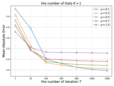
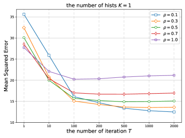
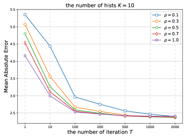
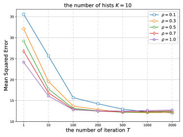
Firstly, we would like to show our surprising finding that ensemble of binary histograms in each iteration of the proposed GBBHE can greatly boost the numerical performance with easier hyper-parameter selection in the empirical aspect. To illustrate this, we vary the number of iteration and the learning rate , fix the depth of binary histograms , and plot the test error curves under different numbers of binary histograms and . Results are shown in Figure 2 and Figure 3 respectively.
In Figure 2, only when the number of iteration is large enough and the learning rate is small enough does the boosted rotated binary histograms without ensemble in each iteration have good performance. This verifies the common phenomenon that there is a trade-off between the number of iterations and the learning rate in gradient boosting. However, it is very difficult to determine the optimal and because the trade-off is quite sensitive when the number of hists .
By contrast, when ensemble is introduced in each iteration of boosted rotated binary histograms, e.g., , the trade-off between the number of iteration and the learning rate is much less sensitive, see Figure 3 in detail. Although the performance of GBBHE will slightly worse when and become too large, i.e, the trade-off between the number of iteration and the learning rate illustrated in Figure 2 also exists, we find that the performance is satisfactory among a wide range of and . Moreover, it is well worth mentioning that the boosting performance when converges faster than that of compared with Figure 2, resulting in better performance. This exactly corresponds to the theoretical result in Theorem 16 that ensemble can reduce the number of iterations to achieve the fast convergence rate. To conclude, the introduced ensemble with not only stabilizes the hyper-parameter selection of and , but also boosts the convergence of the boosting algorithm.
4.1.2 Parameter Analysis about the Learning Rate
Secondly, we would like to discuss the tendency of the learning rate among different number of iterations . We fix the number of binary histograms and the depth of binary histograms , and then vary the choice of the learning rate among four different .
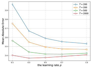
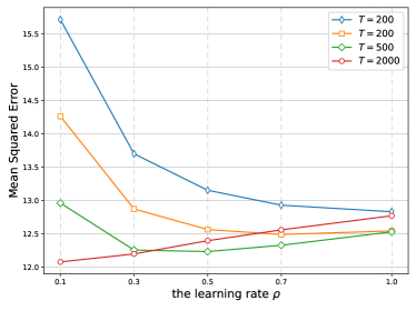
From Figure 4 we see that the test error decreases to an optimal value and then increases as the learning rate increases from to . Besides, we observe that the optimal varies by different numbers of iterations. To be specific, smaller leads to larger optimal , while the optimal goes down with larger . For example, the optimal when is , while the optimal when is . Moreover, as the number of iteration goes up, the test error under optimal consistently decreases, which shows empirically that larger with smaller yields better numerical performance.
4.1.3 Parameter Analysis about the Number of Binary Histograms
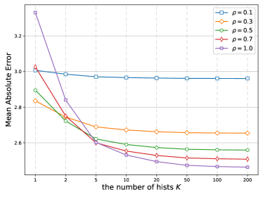
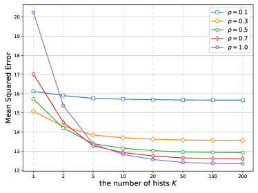
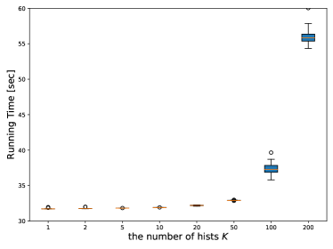
Secondly, we discuss the choice of the number of binary histograms , which controls how ensemble is used in the algorithm GBBHE: larger means more binary histograms built in each iteration of boosting. To be specific, we fix the number of iterations and the depth of binary histograms , and then vary among different learning rates .
Figure 5 and Figure 6 show the accuracy performances and the running times under different numbers of binary histograms respectively. As is shown, on the one hand, as goes up, the performances of regression continue to rise, only with the cost of higher computation times. On the other hand, the marginal increase of performance drops as becomes larger. This phenomenon is consistent regardless of the learning rate varies. Therefore, considering the trade-off between accuracy and running time, shows a satisfactory performance with tolerable running time. Moreover, Figure 5 suggests that ensemble is especially beneficial for large learning rate . This to some extent corresponds to the numerical result shown in Section 4.1.2 that ensemble helps improve performance and the stability of .
4.1.4 Parameter Analysis about the Depth of Binary Histograms
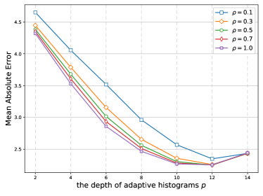
One more hyper-parameter we need to discuss is the depth of binary histograms . The depth controls the denseness of binary histogram partition: the total cells of each binary histogram is , and larger means more partitions for each binary histogram. To numerically analyze the effect of different depths of binary histograms , we fix the number of iterations and the number of binary histograms in each iteration , and vary the depth among different learning rate .
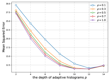
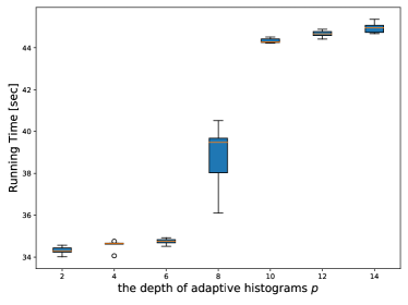
Figure 7 and Figure 8 show the accuracy performances and the running times under different depths of binary histograms respectively. As the depth increases, the accuracy performance first goes up and reaches its optimum, and then deteriorates when the depth of binary histograms becomes too large, with the running time monotonically increasing. This phenomenon is consistent regardless of the learning rate varies. It may attribute to the fact that splitting more in each binary histogram helps to build up binary histograms with local adaptivity, but if is too large, the partitions of binary histograms will be too dense and it is at the risk of over-fitting. Besides, it would be too time-consuming to adopt such large . This also verifies the theoretical results in Theorem 14 and 16 that there exists an optimal order of depth .
4.2 Numerical Comparisons
In this subsection, we conduct numerical studies to evaluate the effectiveness of our proposed Gradient Boosting Binary Histogram Transforms Ensemble (GBBHE) algorithm on moderate and large-scale real data sets. In this part, we consider the rotation transform as an option, i.e., we compare both GBBHE without random rotation (GBBHE w.o. Rotation) and standard GBBHE with random rotation (GBBHE w. Rotation) as is shown in Algorithm 3 with other state-of-the-art large-scale regression algorithms.
4.2.1 Experimental Setups
Comparisons are conducted among
-
•
Gradient Boosting Regression Tree (GBRT): Gradient Boosting Regression Trees is a well-known ensemble method for regression proposed by Friedman (2001). However, different from random forest, trees in GBRT are fitted in a sequential manner. We use the scikit-learn implementation in Python. Three hyper-parameters are considered, including the number of iteration times , learning rate shrinking the contribution of each tree , and the minimum number of samples required to split an internal node min_samples_split. We use a validation set containing of the training samples to find the best , , and .
-
•
Random Forest: Random forest is a well-known ensemble algorithm for regression proposed by Breiman (2001). As each tree is fitted in parallel, random forest is naturally suitable in large-scale applications. We use the scikit-learn implementation in Python. Two hyper-parameters are the number of estimators in the forest and the minimum number of samples required to split an internal node min_samples_split. We use a validation set containing of the training samples to find the best and .
-
•
LiquidSVM: Support vector machines for regression being a global algorithm is impeded by super-linear computational requirements in terms of the number of training samples in large-scale applications. To address this, Meister and Steinwart (2016) employs a spatially oriented method to generate the chunks in feature space, and fit LS-SVMs for each local region using training data belonging to the region. This is called the Voronoi partition support vector machine (VP-SVM). We use the implementation provided by the authors in Python. In each local region, we conduct five-fold cross-validation (CV) to find the best hyper-parameters and .
As for the hyper-parameter tuning of our method, we use a validation set to find the number of iterations , the number of binary histograms , best learning rate and the best depth parameter .
For moderate-sized datasets, we also randomly split of the data set for training and the other for testing. We scale each feature individually to the range on the training set. Hyper-parameters are selected by validation and experiments are repeated times. For the large-scale data sets, the partition of the training set and the testing set is specified in their detailed descriptions in Section 4.2.2, and we repeat the experiments times. We record and summarize the average and the standard deviation of the mean squared error, the mean absolute error, and the running time under the best hyper-parameter setting over all experiments. All experiments are conducted on a 64-bit machine with 40-cores Intel Xeon 2.0GHz CPU (E5-4620) and 256GB main memory.
4.2.2 Description of Datasets
We use for the evaluation seven moderate-sized datasets and five well-known large-scale datasets from the UCI machine learning repository (Dua and Graff, 2017), LIBSVM Data111LIBSVM Data: Classification, Regression, and Multi-label. https://www.csie.ntu.edu.tw/~cjlin/libsvmtools/datasets/, and Delve Datasets222Delve Datasets: Collections of data for developing, evaluating, and comparing learning methods. https://www.cs.toronto.edu/~delve/data/datasets.html. Details of these data sets, including size and dimension, are summarized in Table 1.
| datasets | size | dimension | |
|---|---|---|---|
| Moderate-sized | EGS | ||
| AEP | |||
| CAD | |||
| SCD | |||
| HPP | |||
| ONP | |||
| PTS | |||
| Large-scale | MSD | ||
| BUZ | |||
| GHG | |||
| GTM | |||
| DGM |
-
•
EGS: The Electrical Grid Stability Simulated Data Set (EGS) (Arzamasov et al., 2018) is available on the UCI Machine Learning Repository. It contains samples in total. attributes are used to predict the maximal real part of the characteristic equation root.
-
•
AEP: The Appliances Energy Prediction Data Set (AEP) (Candanedo et al., 2017), available on UCI Machine Learning Repository, contains samples of dimension with attribute “date” removed from the original data set. The data is used to predict the appliances energy use in a low-energy building.
-
•
CAD: The California Housing Prices Data Set (CAD) is avaliable on the LIBSVM Data. This spacial data can be traced back to Pace and Barry (1997). It consists observations on housing prices with economic covariates. Note that for the sake of clarity, all house prices in the original data set have been modified to be counted in thousands.
-
•
SCD: The Superconductivity Data Set (SCD) (Hamidieh, 2018), available on the UCI Machine Learning Repository, is supported by the NIMS, a public institution based in Japan. This database has samples with features. The goal is to predict the critical temperature based on the features extracted.
-
•
HPP: The House Price Prototask Data Set (HPP) is originally taken from the census-house dataset in the DELVE Datasets. We use the house-price-8H prototask, which contains observations. We use features to predict the median house prices from US census data. Similar to the data preprocessing for CAD, all house prices in the original data set have been modified to be counted in thousands.
-
•
ONP: The Online News Popularity Data Set (ONP) (Fernandes et al., 2015), available on the UCI Machine Learning Repository, is a database summarizing a heterogeneous set of features about articles published by Mashable in a period of two years. It contains observations with predictive attributes. This data set is used to predict the number of shares of the online news.
-
•
PTS: Physicochemical Properties of Protein Tertiary Structure Data Set () is available on the UCI Machine Learning Repository. It contains samples of dimension . The regression task is to predict the size of the residue.
-
•
MSD: The Year Prediction MSD Data Set (MSD) (Bertin-Mahieux et al., 2011) is available on the UCI Machine Learning Repository. It contains training samples and testing samples with attributes, depicting the timbre average and timbre covariance of songs released between the years 1922 and 2011. The main task is to learn the audio features of a song and to predict its release year.
-
•
BUZ: Buzz in Social Media Data Set (BUZ) (Kawala et al., 2013) is available on the UCI Machine Learning Repository. It contains examples of buzz events from two different social networks: Twitter, and Tom’s Hardware. We select the Twitter part, which contains samples of dimension and the last column is for prediction. We use the first samples for training, and use the remaining samples for testing.
-
•
GHG: The Greenhouse Gas Observing Network Data Set (GHG) (Lucas et al., 2015) is available on the UCI Machine Learning Repository. It contains samples of dimension , which are time series of GHG tracers released from distinct spatial regions in California and one outside of California. The main task is to predict emissions of greenhouse gas. We use the first samples for training, and use the remaining samples for testing.
-
•
GTM: The Gas Sensor Array Temperature Modulation Data Set (GTM) (Burgués et al., 2018; Burgués and Marco, 2018) is available on the UCI Machine Learning Repository. We use the readings of temperature-modulated metal oxide semiconductor gas sensors, a temperature sensor, and a humidity sensor, as well as the values of mass flow rate and the heater voltage to predict the concentration level of CO. The total number of samples is and the feature dimension is . We use the first samples for training and the remaining samples for evaluation.
-
•
DGM: The Gas Sensor Array Under Dynamic Gas Mixtures Data Set (DGM) (Fonollosa et al., 2015) is available on the UCI Machine Learning Repository. Two gas mixtures are generated in this data set: Ethylene and Methane in air, and Ethylene and CO in air. We select the ethylene-CO mixture in the experimental section, with samples in total. We use readings of chemical sensors to predict the concentration level of CO. In the experiments, we use the first samples for training and the remaining samples for testing.
4.2.3 Results
The comparing results of the average MSE and MAE on seven moderate datasets EGS, AEP, CAD, SCD, HPP, ONP, PTS and five large-scale datasets MSD, BUZ, GHG, GTM, and DGM are presented in Figures 2 and 3. Moreover, we point out that the Wilcoxon test for paired samples with significance level are applied.
| Ours (w.o. Rotation) | Ours (w. Rotation) | Random Forest | LiquidSVM | GBRT | |
|---|---|---|---|---|---|
| EGS | |||||
| AEP | |||||
| CAD | |||||
| SCD | |||||
| HPP | |||||
| ONP | |||||
| PTS | |||||
| MSD | |||||
| BUZ | |||||
| GNG | |||||
| GTM | |||||
| DGM |
-
•
* The best results are marked in bold, and the standard deviation is reported in the parenthesis beside each value.
| Ours (w.o. Rotation) | Ours (w. Rotation) | Random Forest | LiquidSVM | GBRT | |
|---|---|---|---|---|---|
| EGS | |||||
| AEP | |||||
| CAD | |||||
| SCD | |||||
| HPP | |||||
| ONP | |||||
| PTS | |||||
| MSD | |||||
| BUZ | |||||
| GNG | |||||
| GTM | |||||
| DGM |
-
•
* The best results are marked in bold, and the standard deviation is reported in the parenthesis under each value.
| Algorithms | MSE | MAE | Running Time |
|---|---|---|---|
| Ours (w.o. Rotation), , | |||
| Ours (w.o. Rotation), , | |||
| Ours (w. Rotation), , | |||
| Ours (w. Rotation), , | |||
| Random Forest, | |||
| Random Forest, | |||
| Random Forest, | |||
| LiquidSVM | |||
| GBRT, | |||
| GBRT, | |||
| GBRT, |
| Algorithms | MSE | MAE | Running Time |
|---|---|---|---|
| Ours (w.o. Rotation), , | |||
| Ours (w.o. Rotation), , | |||
| Ours (w. Rotation), , | |||
| Ours (w. Rotation), , | |||
| Random Forest, | |||
| Random Forest, | |||
| Random Forest, | |||
| LiquidSVM | |||
| GBRT, | |||
| GBRT, |
| Algorithms | MSE | MAE | Running Time |
|---|---|---|---|
| Ours (w.o. Rotation), , | |||
| Ours (w.o. Rotation), , | |||
| Ours (w. Rotation), , | |||
| Ours (w. Rotation), , | |||
| Random Forest, | |||
| Random Forest, | |||
| Random Forest, | |||
| LiquidSVM | |||
| GBRT, | |||
| GBRT, |
In Tables 2 and 3, we observe that our method with the optimal rotation strategy can reach the comparable or even the best performance in many moderate-sized and large-scale datasets. Here we take the rotation transform as an option, where we can select the best strategy through validation in practice. At a significance level of , our method is significantly different from other methods in most cases. This means that with the combination of boosting and ensemble, we come to a conclusion that our method shows promising performance compared to the efficient algorithms such as boosting-based algorithm GBRT, forest-based algorithm Random Forest, and kernel-based algorithm LiquidSVM.
Furthermore, Table 4, 5, and 6 record the MSE, MAE, and running time performance of each method under different parameter settings on three large-scale data sets MSD, GTM and DGM. It can be seen in the tables that our GBBHE algorithm significantly outperforms other compared methods w.r.t. accuracy. Yet the running time of our method, with rotation or not, is comparable among other algorithms in large-scale circumstances. For example, on MSD, the running time our GBBHE algorithm (w.o. Rotation) with and is comparable with Random Forest () and GBRT (). Nonetheless, the MSE of our GBBHE (w.o. Rotation) is less than Random Forest () and is less than GBRT (). On the other hand, when compared with GBRT, our method turns out to converge faster. For example, on the GTM dataset, the MSE of our GBBHE (w.o. Rotation) drops by only when changes from to , while the MAE is nearly the same, which indicates convergence of our algorithm. By contrast, the MSE of GBRT decreases by a large margin from to when changes from to . Besides, the MAE decreases from to . Moreover, despite with , where more running time is consumed, GBRT still shows worse performance than our GBBHE (w.o. Rotation). This exactly demonstrates the faster convergence to a better performance of our algorithm.
5 Comments and Discussions
5.1 Comparisons with the Prior Work
In the prior work of this paper (Cai et al., 2020), we take ordinary histogram transforms as the base learner in the gradient boosting algorithm and proposed the Boosted Histogram Transform for Regression (BHTR). The convergence rate is proved to be in the space and in the space . Moreover, a lower bound of convergence rates for the base learner is proved to be which demonstrates the advantage of boosting. In this paper, we take a step further to analyze the behavior of an algorithm that applies better to the regression problem with large-scale and especially high-dimensional data. To be specific, we introduce additional randomness to GBBH by utilizing the rotated binary histogram as the base learner and manage to derive fast convergence in the Hölder function space. Unfortunately, the GBBH converges slightly slower than BHTR. However, it is worth pointing out that the major shortcoming of ordinary histogram partition is that the number of splits grows exponentially with dimension . Thus, it is difficult for BHTR to apply to high-dimensional data. Therefore, in this paper, we adopt the binary histogram partition to deal with this problem, and further use the ensemble method to improve the computational efficiency for large-scale regression.
5.2 Comments on Theoretical Results
Previous theoretical works about boosting algorithms for regression include Bühlmann and Yu (2003) and Lin et al. (2019), where linear regressors and kernel ridge regressors are used as the base learners. These works analyze the learning performance by using the integral operator approach and prove the optimal convergence rate. However, this analysis turns out to be inapplicable to our method. In this paper, we conduct analysis under the framework of regularized empirical risk minimization (RERM).
Throughout the ensemble learning algorithms, perhaps the most related work to ours is Biau (2012), where they investigate a random forest model with a midpoint splitting rule which coincides with the construction procedure of our binary histogram. The convergence rate of their proposed algorithm is proved to be in the space . As for this paper, the convergence rate of our GBBH when the target function lies in the space turns out to be , slower than that of Biau (2012)’s. However, for smoother functions in the subspace , the convergence rate of GBBH is actually faster than that of Biau (2012)’s when , which indicates that our GBBH can deal better with smoother target functions.
5.3 Comments on Large-scale Regression
In the literature, there have been many efforts on solving the large-scale regression problem. For example, the mainstream solutions fall into two categories, the horizontal methods and the vertical methods. The former partitions the data set into several disjoint subsets, implements a certain learning algorithm to each data subset to obtain a local predictor, and finally synthesizes a global output. However, this approach suffers from its own inherent disadvantages that the local predictor may be quite different from the global optimal predictor. On the other hand, vertical methods divide the feature space into multiple non-overlapping cells through different partition methods, e.g. Suykens et al. (2002); Espinoza et al. (2006); Biau (2012). Then a predictor is embedded on each partitioning cell, such as Gaussian process regression (Park et al., 2011; Park and Huang, 2016; Park and Apley, 2018), support vector machines (Meister and Steinwart, 2016; Thomann et al., 2017), etc.
In this paper, our algorithm is inspired by the vertical methods. However, we notice that previous vertical methods for large-scale regression usually adopt kernel-based approaches to ensure sound theoretical properties and enhance the performance, especially under high-dimensional scenarios. By contrast, instead of resorting to kernel methods, we achieve comparable or even better performance by combining two ensemble learning methods. Moreover, our algorithm adopts the binary histogram partition, which enjoys high computational efficiency compared with kernel methods even on high-dimensional data. As is shown in Table 2 and 3, GBBHE enjoys the lowest testing error measured by both MSE and MAE. Moreover, our GBBHE turns out to be more computationally efficient than these kernel-based methods. For example, in Table 4, 5, and 6, our method runs faster than the kernel-based LiquidSVM.
Previous works on boosting algorithms for solving large-scale regression often adopt acceleration techniques mainly from the perspective of optimization. For example, in Biau et al. (2019), the computational efficiency is enhanced by incorporating an accelerated gradient descent technique. By contrast, our GBBHE for the first time reduces the computational cost by accelerating the convergence with respect to , which is guaranteed by statistical learning theory. To be specific, we show that in Theorem 16 to achieve the same convergence rate, we require (instead of ) to be of the order . That is, we can enhance the computational efficiency of our proposed gradient boosting algorithm through theoretically proved reduction of the number of iterations .
6 Error Analysis
This section provides more comprehensive error analysis for the theoretical results in Section 3. In Subsection 6.1, we present some fundamental lemmas and propositions for the properties of the binary histogram transform and the sample error analysis. Then, in Subsections 6.2 and 6.3, we conduct approximation error analysis for the boosted regressor under the assumption that the Bayes decision function lies in the Hölder spaces and , respectively.
6.1 Fundamental Lemmas and Propositions
6.1.1 Properties of Binary Histogram Transform
Throughout the proof of this paper, we will make repeated use of the following two facts proposed by Biau (2012).
Fact 20
For , let defined by (5) be the rectangular cell of the rotated binary histogram containing and be the number of times that is split on the -th coordinate () in the transformed space. Then conditionally on the rotation transformation , has binomial distribution with parameters and probability and satisfies
Moreover, let be the size of the -th dimension of in the transformed space. Then we have
| (25) |
where denotes the probability distribution conditionally on the rotation transformation and indicates that variables in the two sides of the equation have the same distribution.
Fact 21
Let be the Lebesgue measure. For , let be the number of samples falling in the same cell as , that is,
By construction, we have
| (26) |
Before we proceed, we present the following lemma, which helps to bound the diameter of the rectangular cell .
Lemma 22
Suppose that , and . Then we have
| (27) |
Combining Lemma 22 with Fact 21, it is easy to derive the following lemma which plays an important role to bound the approximation error of the estimator.
Lemma 23
Let the diameter of the set be defined by
Then for any and , there holds
For any , let and be the minimum and maximum values of the -th entries of points in . Then, by the construction of rotated binary histogram, there holds
The next theorem gives an explicit form of the distance between and the center of the interval , which is used to derive the lower bound for the error of single binary histogram regressor.
Lemma 24
6.1.2 Bounding the Sample Error Term
To derive bounds on the sample error of regularized empirical risk minimizers, let us briefly recall the definition of VC dimension measuring the complexity of the underlying function class.
Definition 25 (VC dimension)
Let be a class of subsets of and be a finite set. The trace of on is defined by . Its cardinality is denoted by . We say that shatters if , that is, if for every , there exists a such that . For , let
| (28) |
Then, the set is a Vapnik-Chervonenkis class if there exists such that and the minimal of such is called the VC dimension of , and abbreviate as .
To prove Lemma 26, we need the following fundamental lemma concerning with the VC dimension of the tree-based partitions of with internal nodes, that is, we use hyper-planes without intersections between each other to split into sub-regions. In fact, the histogram transform partition proposed in Section 2.3 is a binary tree-based partition with internal nodes. The key of the lemma 26 follows the idea put forward by Breiman (2000) of the construction of purely random forest. To this end, let be fixed and be a tree-based partition of with internal nodes.
Lemma 26
Let be defined by
| (29) |
Then the VC dimension of can be upper bounded by .
To investigate the capacity property of continuous-valued functions, we need to introduce the concept VC-subgraph class. To this end, the subgraph of a function is defined by
A class of functions on is said to be a VC-subgraph class, if the collection of all subgraphs of functions in , which is denoted by is a VC class of sets in . Then the VC dimension of is defined by the VC dimension of the collection of the subgraphs, that is, .
Before we proceed, we also need to recall the definitions of the convex hull and VC-hull class. The symmetric convex hull of a class of functions is defined as the set of functions with and each contained in . A set of measurable functions is called a VC-hull class, if it is in the pointwise sequential closure of the symmetric convex hull of a VC-class of functions.
We denote the function set as
| (30) |
which contains all the functions of induced by all possible rotation transformations with the size parameter . The following lemma presents the upper bound for the VC dimension of the function set .
Lemma 27
Let be the function set defined as in (30). Then is a -subgraph class with
To further bound the capacity of the function sets, we need to introduce the following fundamental descriptions which enables an approximation of an infinite set by finite subsets.
Definition 28 (Covering Numbers)
Let be a metric space, and . We call an -net of if for all there exists an such that . Moreover, the -covering number of is defined as
where denotes the closed ball in centered at with radius .
The following lemma follows directly from Theorem 2.6.9 in Van der Vaart and Wellner (1996). For the sake of completeness, we present the proof in Section 7.1.2.
Lemma 29
Let be a probability measure on and
Assume that for some fixed and , the covering number of satisfies
| (31) |
Then there exists a universal constant such that
The next theorem shows that covering numbers of grow at a polynomial rate.
Proposition 30
Let be a function set defined as in (30). Then there exists a universal constant such that for any and any probability measure , we have
The following theorem gives an upper bound on the covering number of the -hull class .
Proposition 31
Let be the function set defined as in (30). Then there exists a constant such that for any and any probability measure , there holds
| (32) |
Next, let us recall the definition of entropy numbers.
Definition 32 (Entropy Numbers)
Let be a metric space, and be an integer. The -th entropy number of is defined as
Moreover, if is a subspace of a normed space and the metric is given by , , we write . Finally, if is a bounded, linear operator between the normed space and , we denote .
It is well-known that entropy numbers are closely related to the covering numbers. To be specific, entropy and covering numbers are in some sense inverse to each other. More precisely, for all constants and , the implication
| (33) |
holds by Lemma 6.21 in Steinwart and Christmann (2008). Additionally, Exercise 6.8 in Steinwart and Christmann (2008) yields the opposite implication, namely
| (34) |
For a finite set , we define the norm of an empirical -space by
If is the function space (8) and , then the entropy number equals the -th entropy number of the symmetric convex hull of the family , where denotes the identity map that assigns to every the corresponding equivalence class in .
6.2 Error Analysis for
First of all, we introduce some definitions and notations. For a given rotated binary histogram and split coordinates , we write
| (35) |
In other words, is the function that minimizes the excess risk over the function set . Then, elementary calculation yields
Moreover, we write
| (36) |
for the empirical version, which can be further presented as
The following proposition shows that the distance between and behaves polynomial in the regularization parameter if we choose the size of binary histogram partition appropriately.
Proposition 33
Let the rotated binary histogram be defined in Algorithm 1 with depth . Moreover, suppose that the Bayes decision function . Then, for any fixed , there holds
where is some constant depending on , and .
6.2.1 Upper Bound of Convergence Rate of GBBH
6.2.2 Upper Bound of Convergence Rate of GBBHE
6.3 Error Analysis for
A drawback to the analysis in is that the usual Taylor expansion involved techniques for error estimation may not apply directly. As a result, we fail to prove the exact benefits of the boosting procedure. Therefore, in this subsection, we turn to the function space consisting of smoother functions. To be specific, we study the convergence rates of to the Bayes decision function . To this end, there is a point in introducing some notations.
For fixed , let be rotated binary histograms with depth and split coordinates , . Moreover, let and be defined as in (35) and (36), respectively. For , we define
| (37) |
and
| (38) |
Moreover, in the scenario of gradient boosted binary histogram ensemble for large-scale regression, we write
| (39) |
Furthermore, we define
| (40) |
and
| (41) |
In particular, for the binary histogram regressor, we are concerned with the lower bound for . In this case, we suppose that is the uniform distribution on . As a result, it is sufficient for us to consider the fixed transformation to apply binary histogram partition on . Consequently, we make the error decomposition
| (42) |
It is important to note that both of the two terms on the right-hand side of (42) are data- and partition-independent due to the expectation with respect to and respectively. Loosely speaking, the first error term corresponds to the expected estimation error of the estimator , while the second one demonstrates the expected approximation error.
6.3.1 Upper Bound of Convergence Rate of GBBH
The next proposition presents the upper bound of the distance between the boosted regressor and the Bayes decision function in the Hölder space .
Proposition 36
Let be defined by (37). Moreover, let the Bayes decision function and be the uniform distribution on . Then we have
| (43) |
6.3.2 Upper Bound of Convergence Rate of GBBHE
The next proposition presents the upper bound of the distance between the boosted rotated binary histogram ensemble and the Bayes decision function in the Hölder space .
Proposition 37
Let be defined by (41). Moreover, let the Bayes decision function and be the uniform distribution on . Then we have
| (44) |
6.3.3 Lower Bound of Convergence Rate of Binary Histogram Regression
The following two propositions present the lower bound of approximation error and sample error of GBBH Regression, respectively.
Proposition 38
Let the rotated binary histogram be defined as in Algorithm 1 with the identity map and the regression model be defined by
| (45) |
with . Furthermore, suppose that is the uniform distribution on and is independent of such that . Moreover, suppose that there exists a fixed constant such that
| (46) |
Then we have
7 Proofs
7.1 Proofs Related to Section 6.1
7.1.1 Proofs Related to Section 6.1.1
Proof [of Lemma 22] For any , it is easy to see that
Since , we have
Consequently, we get
Thus we complete the proof.
Proof [of Lemma 23] By definition, we have
Consequently, (25) in Fact 20 implies
Applying Lemma 22, we get
Therefore, we obtain
Taking expectation with respect to , we prove the desired assertion.
Proof [of Lemma 24] If , by the construction of rotated binary histogram partition, we have
| (47) |
By the definition of , for any , there holds
Since , we have
| (48) |
Therefore, using the triangular inequality, we obtain
This together with (48) implies that
holds for any . Combining this with (47), we get
which leads to the desired assertion.
7.1.2 Proofs Related to Section 6.1.2
Proof [of Lemma 26] This proof is conducted from the perspective of geometric constructions.
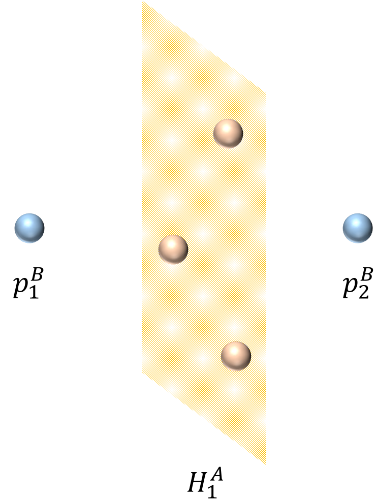
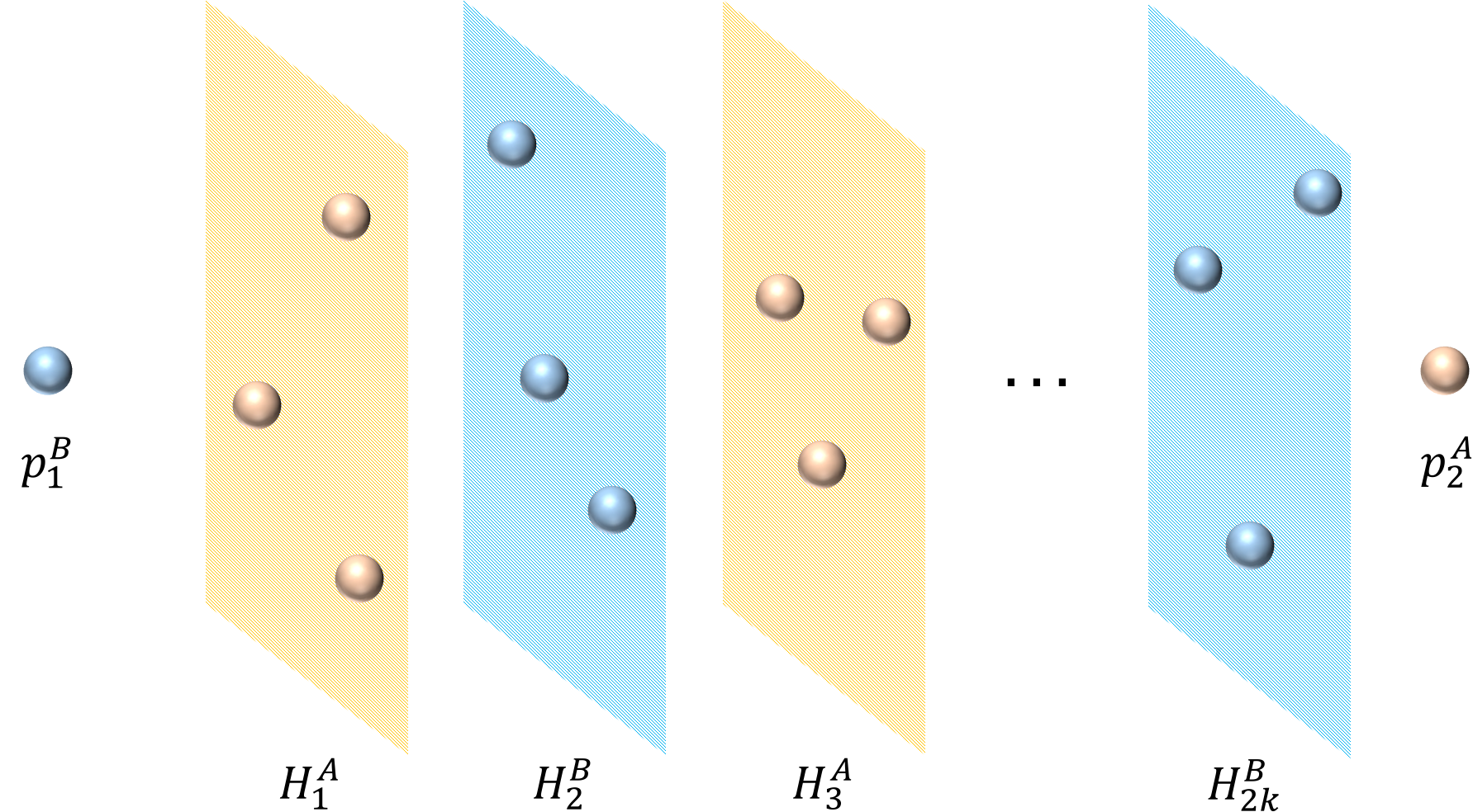
We proceed by induction. Firstly, we concentrate on partition with the number of splits . Because of the dimension of the feature space is , the smallest number of sample points that cannot be divided by split is . Concretely, owing to the fact that points can be used to form independent vectors and hence a hyperplane in a -dimensional space, we might take the following case into consideration: There is a hyperplane consisting of points all from one class, say class , and two points , from the opposite class located on the opposite sides of this hyperplane, respectively. We denote this hyperplane by . In this case, points from two classes cannot be separated by one split (since the positions are ), so that we have .
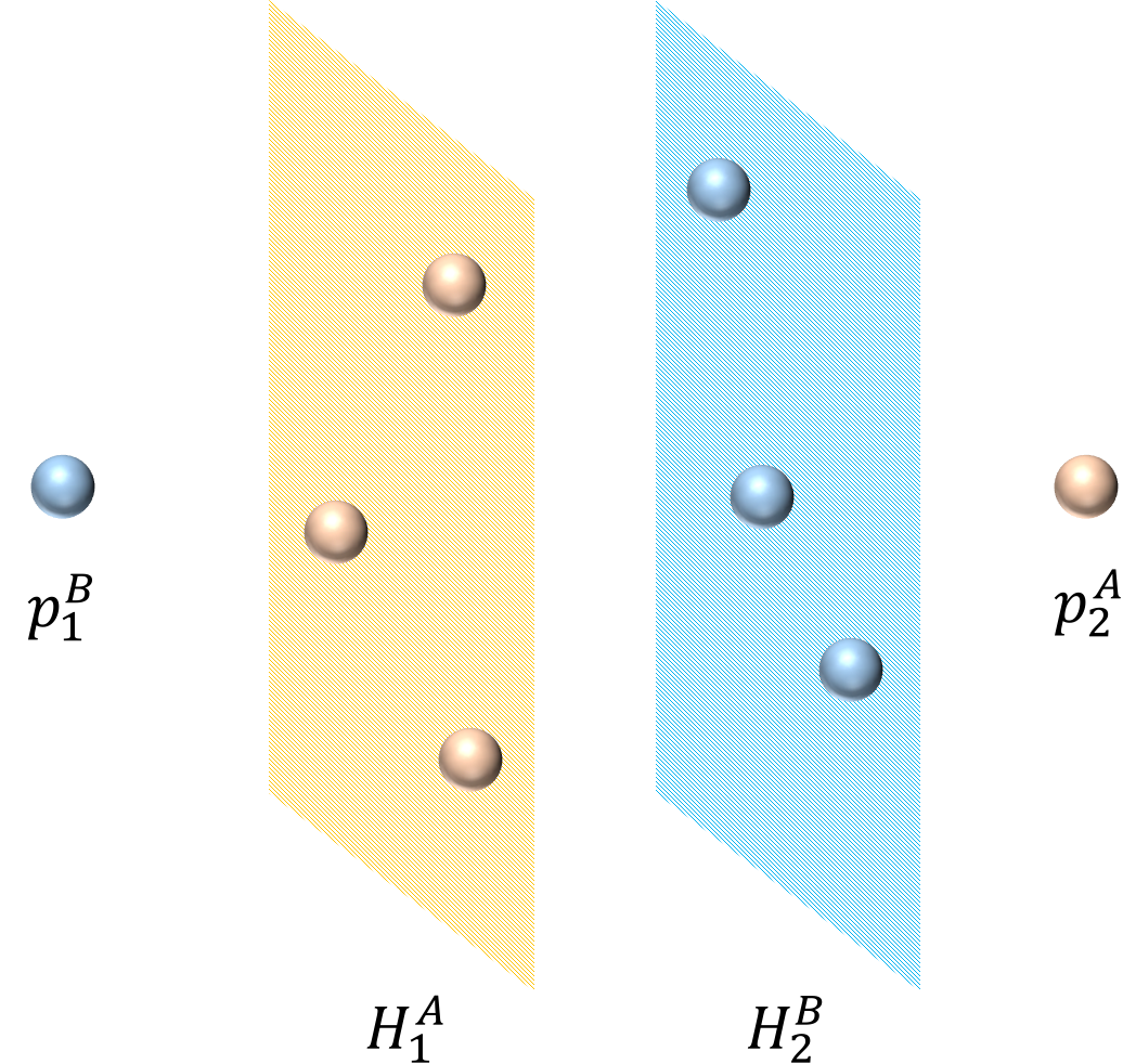
Next, when the partition is with the number of splits , we analyze in the similar way only by extending the above case a little bit. Now, we pick either of the two single sample points located on opposite side of the , and add more points from class to it. Then, they together can form a hyperplane parallel to . After that, we place one more sample point from class to the side of this newly constructed hyperplane . In this case, the location of these two single points and two hyperplanes are . Apparently, splits cannot separate these points. As a result, we have .
Inductively, the above analysis can be extended to the general case of number of splits . In this manner, we need to add points continuously to form mutually parallel hyperplanes where any two adjacent hyperplanes should be constructed from different classes. Without loss of generality, we consider the case for , , where two points (denoted as , ) from class and alternately appearing hyperplanes form the space locations: .
Accordingly, the smallest number of points that cannot be divided by splits is , leading to . This completes the proof.
Proof [of Lemma 27] Recall that for an histogram transform splitting rule, we construct the binary tree-based partition on the hypercube with depth , which leads to internal nodes of the partition. Consequently, applying lemma 26, we get
Thus we complete the proof.
Proof [of Lemma 29] Let be an -net over . Then, for any , there exists an such that . Therefore, we can assume without loss of generality that is finite.
Obviously, (31) holds for . Let and . Then (31) implies that for any , there exists such that for any , there exists an such that
Therefore, for each , we can find sets such that the set is a -net over and .
In the following, we show by induction that for and , there holds
| (49) |
where and are constants depending only on and such that . The proof of (49) will be conducted by a nested induction argument.
Let us first consider the case . For a fixed , let . Then for satisfying , there holds
which immediately implies (49). For a general , let for large enough to be chosen later. Then for any , there exists an such that
Let be the projection operator. Then for any , there holds
Therefore, for and , we have
Let be the set
Then we have and for any , there holds
Moreover, we have
| (50) |
Applying Lemma 2.6.11 in Van der Vaart and Wellner (1996) with to , we can find a -net over consisting of at most
| (51) |
elements.
Suppose that (49) holds for and . In other words, there exists a -net over consisting of at most elements, which partitions into -dimensional cells of diameter at most . Each of these cells can be isometrically identified with a subset of a ball of radius in and can be therefore further partitioned into
cells of diameter . As a result, we get a -net of containing at most
| (52) |
elements.
Now, (50) together with (51) and (52) yields that there exists a -net of whose cardinality can be bounded by
for suitable choices of and depending only on . This concludes the proof of (49) for and every .
Let us consider a general . Similarly as above, there holds
| (53) |
where the set contains at most elements with norm smaller than . Applying Lemma 2.6.11 in Van der Vaart and Wellner (1996) to , we can find an -net over consisting of at most
| (54) |
elements. Moreover, by the induction hypothesis, we have a -net over consisting of at most
| (55) |
elements. Using (53), (54), and (55), we obtain a -net over consisting of at most elements, where
Form the elementary analysis we know that if , then there exist constants , , and such that
Thus (49) is proved. Taking in (49), we get
This together with
yields
where the constant depends on the constants , and .
This finishes the proof.
7.2 Proofs for
Proof [of Proposition 33] The assumption implies that for any , there holds
Therefore, we get
Consequently we obtain
Applying Lemma 23, we get
by choosing
where the constant .
7.2.1 Proofs Related to Section 6.2.1
Proof [of Theorem 34] Denote
and for , we write
Note that for , we have , that is,
Then, by the Cauchy-Schwarz inequality, we get
Consequently, we have . Since is Lipschitz continuous with , we find
Let , , and . Then (32) together with (34) implies that
Taking expectation with respect to , we get
| (56) |
where . Moreover, we easily find
Therefore, (56) can be further estimated by
which leads to
For the least square loss, the superemum bound
and the variance bound
holds for and . Therefore, for , we have
Then Theorem 7.16 in Steinwart and Christmann (2008) with yields that there exist a constant such that
Simple algebra shows that the condition is satisfied. Since , similar arguments show that there still hold the statements of the Peeling Theorem 7.7 in Steinwart and Christmann (2008). Consequently, Theorem 7.20 in Steinwart and Christmann (2008) can also be applied, if the assumptions on and are modified to and , respectively. It is easy to verify that the condition is satisfied if
where is a constant, which yields the assertion.
7.2.2 Proofs Related to Section 6.2.2
Proof [of Theorem 35] Denote
and for , we write
Note that for , we have , that is,
Then, by the Cauchy-Schwarz inequality, we get
Consequently, we have . Since is Lipschitz continuous with , we find
By the definition of in (17), we have . Consequently, we find
Through the similar arguments in the proof of Theorem 34, we are able to obtain the desired assertion. Thus, we omit the details here.
7.2.3 Proofs Related to Section 3.2
Proof [of Theorem 5] It is easy to see that defined by (37) satisfies and . Moreover, by Jensen’s inequality, we have
Combining this with Proposition 33, we obtain
Consequently we get
Then Theorem 34 implies that with probability not less than , there holds
| (57) |
where , and are constants defined as in Proposition 33 and Theorem 34. Minimizing the right hand side of (57), we get
| (58) |
if we choose
where is a constant depending on , , , , and . Consequently, by the Borel-Cantelli Lemma, (58) holds with probability equal to one for sufficiently large , which leads to the desired assertion.
7.2.4 Proofs Related to Section 3.4
Proof [of Theorem 14] It is easy to see that defined by (41) satisfies and . Moreover, by Jensen’s inequality, we have
Combining this with Proposition 33, we obtain
Consequently we get
Then, Theorem 35 implies that with probability not less than , there holds
| (59) |
where , and are constants defined as in Proposition 33 and Theorem 34. Minimizing the right hand side of (57), we get
| (60) |
if we choose
where is a constant depending on , , , , and . Consequently, by the Borel-Cantelli Lemma, (58) holds with probability equal to one for sufficiently large , which leads to the desired assertion.
7.3 Proofs for
7.3.1 Proofs Related to Section 6.3.1
Proof [of Proposition 36] According to the rotated binary histogram splitting rule, the rotation transformation and split coordinates are i.i.d. Therefore, for any , the expected approximation error term can be decomposed as follows:
| (61) |
For the first term in (61), the assumption implies
| (62) |
According to Lemma 23, the first term is further bounded by
| (63) |
We now consider the second term in (61). Taking the first-order Taylor expansion of at , we get
| (64) |
Therefore, there holds
Now, by the triangle inequality, we have
Then we get
| (65) |
where is a constant. By making the substitution and writing , we obtain
| (66) |
Since we have , recall that is a orthogonal matrix, thus we find
Together with (7.3.1), we find
| (67) |
where and denote the -th entries of the vectors and respectively.
Recall that and denotes the minimum and maximum values of the -th entries of points in . Moreover, by the construction of rotated binary histogram, there holds
Since , we have for any and . Consequently, we get
| (68) |
where we use the fact that an orthogonal transformation is volume-preserving. Combining (67) with (7.3.1), we obtain
| (69) |
Then (7.3.1) together with (7.3.1) yields
Combining this with (7.3.1), we obtain
| (70) |
By (25), we have
| (71) |
Moreover, Lemma 23 implies
| (72) |
Combining (71), (72) with (70), we get
| (73) |
Combining (63), (7.3.1) with (61), we find
Taking expectation with respect to , we get
which leads to the desired assertion by exchanging the order of integration.
7.3.2 Proofs Related to the Upper Bound in Section 3.3
Proof [of Theorem 9] It is easy to see that defined by (37) satisfies and . Then we have
Applying Proposition 36, we find
This together with Theorem 34 implies that with probability at least , there holds
where and . Choosing
we obtain that with probability not less than , there holds
Consequently, by the Borel-Cantelli Lemma, (22) holds with probability equal to one for sufficiently large . This completes the proof.
7.3.3 Proofs Related to Section 3.5
Proof [of Theorem 16] It is easy to see that defined by (41) satisfies and . Then we have
Applying Proposition 36, we find
This together with Theorem 35 implies that with probability at least , there holds
where and . Choosing
we obtain that with probability not less than , there holds
Consequently, by the Borel-Cantelli Lemma, (24) holds with probability equal to one for sufficiently large . This completes the proof.
7.3.4 Proofs Related to Section 6.3.2
Proof [of Proposition 37] According to the rotated binary histogram splitting rule, the rotation transformation and split coordinates , , are i.i.d. Therefore, for any , the expected approximation error term can be decomposed as follows:
| (74) |
Combining (74) with (63) and (7.3.1), we find
Taking expectation with respect to , we get
which leads to the desired assertion by exchanging the order of integration.
7.3.5 Proofs Related to Section 6.3.3
We first show proofs for lower bound of approximation error for binary histogram regression.
Proof [of Proposition 38] Recall that the regression model is defined as . Considering the case when has the uniform distribution, for any and , we have
Since , according to the mean-value theorem, there exists such that
Consequently, we have
| (75) |
Let , . Since , is differentiable at every . According to Lagrange’s mean value theorem, there exists such that
Let . Then we have
Since , we have
Combining this with (7.3.5), we get
| (76) |
where denotes the -th entry of the vector . Let and be the minimum and maximum values of the -th coordinates of points in . Since is an identity map, by the construction of the binary histogram partition, we have
Moreover, let . Then by the iterated integral rule, we have
Consequently, we get
This together with (7.3.5) implies
where and are the minimum and maximum values of the -th coordinates of points in . Therefore, we obtain
| (77) |
Let be the number of times that is split on the -th coordinate. According to Lemma 24, if , , then we have
where
Therefore, we obtain
This together with (77) implies
| (78) |
where . By the definition of , we have
This together with (7.3.5) implies
which completes the proof.
Then we present proofs for lower bound of sample error for binary histogram regression.
Proof [of Proposition 39] Since is a identity map, for any fixed split coordinates , forms a partition of , then for we define the random variable by
Since the random variables are i.i.d. Bernoulli distributed with parameter , it is clear to see that the random variable is Binomial distributed with parameters and . Therefore, for any , we have
Moreover, the GBBH regressor can be defined by
By the law of total probability, we get
| (79) | |||
| (80) |
For the term (79), we have
Since for a fixed , there holds
| (81) |
Moreover, for any fixed , there holds
Consequently, we obtain
Therefore, we get
Clearly, is convex for . Therefore, by Jensen’s inequality, we get
where the last inequality follows from , . Therefore, we have
| (82) |
where we use the fact that for by (26) and is the uniform distribution on .
7.3.6 Proofs Related to the Lower Bound in Section 3.3
Proof [of Theorem 12] Recall the error decomposition (42). Applying Propositions 38 and 39, we get
If , we have
| (84) |
where the constant . On the other hand, we turn to the case . Let , , we find . It is easy to see that when and when , which yields that is increasing on the interval and decreasing on the interval . Therefore, for , there holds
Consequently, we get
| (85) |
Combining (84) with (7.3.6), we find
which leads to the desired assertion.
References
- Arzamasov et al. (2018) Vadim Arzamasov, Klemens Böhm, and Patrick Jochem. Towards concise models of grid stability. In 2018 IEEE International Conference on Communications, Control, and Computing Technologies for Smart Grids (SmartGridComm), pages 1–6. IEEE, 2018.
- Bertin-Mahieux et al. (2011) Thierry Bertin-Mahieux, Daniel P.W. Ellis, Brian Whitman, and Paul Lamere. The million song dataset. In Proceedings of the 12th International Conference on Music Information Retrieval (ISMIR 2011), 2011.
- Biau (2012) Gérard Biau. Analysis of a random forests model. The Journal of Machine Learning Research, 13(1):1063–1095, 2012.
- Biau et al. (2019) Gérard Biau, Benoît Cadre, and Laurent Rouvìère. Accelerated gradient boosting. Machine Learning, 108(6):971–992, 2019.
- Blanchard et al. (2003) Gilles Blanchard, Gábor Lugosi, and Nicolas Vayatis. On the rate of convergence of regularized boosting classifiers. The Journal of Machine Learning Research, 4(Oct):861–894, 2003.
- Blaser and Fryzlewicz (2016) Rico Blaser and Piotr Fryzlewicz. Random rotation ensembles. The Journal of Machine Learning Research, 17(1):126–151, 2016.
- Breiman (2000) Leo Breiman. Some infinity theory for predictor ensembles. Technical report, Technical Report 579, Statistics Dept. UCB, 2000.
- Breiman (2001) Leo Breiman. Random forests. Machine Learning, 45(1):5–32, 2001.
- Bühlmann and Yu (2003) Peter Bühlmann and Bin Yu. Boosting with the loss: regression and classification. Journal of the American Statistical Association, 98(462):324–339, 2003.
- Burgués and Marco (2018) Javier Burgués and Santiago Marco. Multivariate estimation of the limit of detection by orthogonal partial least squares in temperature-modulated mox sensors. Analytica chimica acta, 1019:49–64, 2018.
- Burgués et al. (2018) Javier Burgués, Juan Manuel Jiménez-Soto, and Santiago Marco. Estimation of the limit of detection in semiconductor gas sensors through linearized calibration models. Analytica chimica acta, 1013:13–25, 2018.
- Cai et al. (2020) Yuchao Cai, Hanyuan Hang, Hanfang Yang, and Zhouchen Lin. Boosted histogram transform for regression. In International Conference on Machine Learning, pages 1251–1261. PMLR, 2020.
- Candanedo et al. (2017) Luis M Candanedo, Véronique Feldheim, and Dominique Deramaix. Data driven prediction models of energy use of appliances in a low-energy house. Energy and buildings, 140:81–97, 2017.
- Chen and Guestrin (2016) Tianqi Chen and Carlos Guestrin. XGBoost: A scalable tree boosting system. In Proceedings of the 22nd ACM SIGKDD International Conference on Knowledge Discovery and Data Mining, pages 785–794, 2016.
- Dua and Graff (2017) Dheeru Dua and Casey Graff. UCI machine learning repository, 2017.
- Dubout and Fleuret (2014) Charles Dubout and François Fleuret. Adaptive sampling for large scale boosting. The Journal of Machine Learning Research, 15(1):1431–1453, 2014.
- Espinoza et al. (2006) Marcelo Espinoza, Johan A.K. Suykens, and Bart De Moor. Fixed-size least squares support vector machines: a large scale application in electrical load forecasting. Computational Management Science, 3(2):113–129, 2006.
- Fernandes et al. (2015) Kelwin Fernandes, Pedro Vinagre, and Paulo Cortez. A proactive intelligent decision support system for predicting the popularity of online news. In Portuguese Conference on Artificial Intelligence, pages 535–546. Springer, 2015.
- Fonollosa et al. (2015) Jordi Fonollosa, Sadique Sheik, Ramón Huerta, and Santiago Marco. Reservoir computing compensates slow response of chemosensor arrays exposed to fast varying gas concentrations in continuous monitoring. Sensors and Actuators B: Chemical, 215:618–629, 2015.
- Freund (1995) Yoav Freund. Boosting a weak learning algorithm by majority. Information and computation, 121(2):256–285, 1995.
- Freund and Schapire (1997) Yoav Freund and Robert E Schapire. A decision-theoretic generalization of on-line learning and an application to boosting. Journal of Computer and System Sciences, 55(1):119–139, 1997.
- Friedman (2001) Jerome H Friedman. Greedy function approximation: a gradient boosting machine. The Annals of Statistics, 29(5):1189–1232, 2001.
- Hamidieh (2018) Kam Hamidieh. A data-driven statistical model for predicting the critical temperature of a superconductor. Computational Materials Science, 154:346–354, 2018.
- Kawala et al. (2013) François Kawala, Ahlame Douzal-Chouakria, Eric Gaussier, and Eustache Dimert. Prédictions d’activité dans les réseaux sociaux en ligne. In 4ième conférence sur les modèles et l’analyse des réseaux: Approches mathématiques et informatiques, page 16, 2013.
- Ke et al. (2017) Guolin Ke, Qi Meng, Thomas Finley, Taifeng Wang, Wei Chen, Weidong Ma, Qiwei Ye, and Tie-Yan Liu. LightGBM: A highly efficient gradient boosting decision tree. In Proceedings of the 30th International Conference on Neural Information Processing Systems, volume 30, pages 3146–3154, 2017.
- Lin et al. (2019) Shao-Bo Lin, Yunwen Lei, and Ding-Xuan Zhou. Boosted kernel ridge regression: Optimal learning rates and early stopping. The Journal of Machine Learning Research, 20(46):1–36, 2019.
- López-Rubio (2013) Ezequiel López-Rubio. A histogram transform for probabilitydensity function estimation. IEEE Transactions on Pattern Analysis and Machine Intelligence, 36(4):644–656, 2013.
- Lucas et al. (2015) DD Lucas, C Yver Kwok, P Cameron-Smith, H Graven, D Bergmann, TP Guilderson, R Weiss, and R Keeling. Designing optimal greenhouse gas observing networks that consider performance and cost. Geoscientific Instrumentation, Methods and Data Systems, 4(1):121–137, 2015.
- Meister and Steinwart (2016) Mona Meister and Ingo Steinwart. Optimal learning rates for localized SVMs. The Journal of Machine Learning Research, 17(194):1–44, 2016.
- Nesterov (1983) Yu E Nesterov. A method of solving a convex programming problem with convergence rate . Dokl. Akad. Nauk SSSR, 269(3):543–547, 1983.
- Pace and Barry (1997) R. Kelley Pace and Ronald Barry. Sparse spatial autoregressions. Statistics and Probability Letters, 33(3):291– 297, 1997.
- Park et al. (2009) BU Park, YK Lee, and S Ha. boosting in kernel regression. Bernoulli, 15(3):599–613, 2009.
- Park and Apley (2018) Chiwoo Park and Daniel Apley. Patchwork kriging for large-scale Gaussian process regression. The Journal of Machine Learning Research, 19(7), 2018.
- Park and Huang (2016) Chiwoo Park and Jianhua Z. Huang. Efficient computation of Gaussian process regression for large spatial data sets by patching local Gaussian processes. The Journal of Machine Learning Research, 17(174):1–29, 2016.
- Park et al. (2011) Chiwoo Park, Jianhua Z. Huang, and Yu Ding. Domain decomposition approach for fast Gaussian process regression of large spatial data sets. The Journal of Machine Learning Research, 12(May):1697–1728, 2011.
- Schapire (1990) Robert E Schapire. The strength of weak learnability. Machine Learning, 5(2):197–227, 1990.
- Schapire and Freund (1995) Robert E Schapire and Yoav Freund. A decision-theoretic generalization of on-line learning and an application to boosting. In Second European Conference on Computational Learning Theory, pages 23–37, 1995.
- Steinwart and Christmann (2008) Ingo Steinwart and Andreas Christmann. Support Vector Machines. Information Science and Statistics. Springer, New York, 2008.
- Suykens et al. (2002) Johan A.K. Suykens, Tony Van Gestel, Jos De Brabanter, Bart De Moor, and Joos Vandewalle. Least Squares Support Vector Machines. World Scientific, Singapore, 2002.
- Thomann et al. (2017) Philipp Thomann, Ingrid Blaschzyk, Mona Meister, and Ingo Steinwart. Spatial decompositions for large scale SVMs. In Proceedings of the 20th International Conference on Artificial Intelligence and Statistics, volume 54 of Proceedings of Machine Learning Research, pages 1329–1337. PMLR, 2017.
- Van der Vaart and Wellner (1996) Aad W. Van der Vaart and Jon A. Wellner. Weak Convergence and Empirical Processes. Springer Series in Statistics. Springer-Verlag, New York, 1996.