Adversarially Adaptive Normalization for Single Domain Generalization

Abstract

Single domain generalization aims to learn a model that performs well on many unseen domains with only one domain data for training. Existing works focus on studying the adversarial domain augmentation (ADA) to improve the model’s generalization capability. The impact on domain generalization of the statistics of normalization layers is still underinvestigated. In this paper, we propose a generic normalization approach, adaptive standardization and rescaling normalization (ASR-Norm), to complement the missing part in previous works. ASR-Norm learns both the standardization and rescaling statistics via neural networks. This new form of normalization can be viewed as a generic form of the traditional normalizations. When trained with ADA, the statistics in ASR-Norm are learned to be adaptive to the data coming from different domains, and hence improves the model generalization performance across domains, especially on the target domain with large discrepancy from the source domain. The experimental results show that ASR-Norm can bring consistent improvement to the state-of-the-art ADA approaches by $1.6\%$, $2.7\%$, and $6.3\%$ averagely on the Digits, CIFAR-10-C, and PACS benchmarks, respectively. As a generic tool, the improvement introduced by ASR-Norm is agnostic to the choice of ADA methods.

1 Introduction

Deep learning has achieved remarkable success in various areas [25, 28] where the training and test data are sampled from the same domain. In real applications, however, there is a great chance of applying a deep learning model to the data from a new domain unseen in the training dataset. The model that performs well on the training domain often cannot maintain a consistent performance on a new domain [53, 5], due to the cross-domain distributional shift [37]. To address the potential discrepancies between the training and test domains, a number of works [20, 6, 61] have been proposed to learn domain-invariant features using the training data from multiple source domains [45, 30] to improve the model’s generalization capability across domains. However, acquiring multi-domain training data is both challenging and expensive. Alternatively, a more practical but less investigated solution is to train the model on a single source domain data and enhance its capability of generalizing to other unseen domains (see the example in Fig. 1). This emerging learning paradigm is referred to as single domain generalization [42].

Figure 1: Illustration of single domain generalization with the PACS [30] benchmark. The dataset contains $4$ domains: art paint, cartoon, sketch, and photo domains, which share the same categories that include dog, elephant, giraffe, guitar, house, horse, and person. Single domain generalization aims at training a model on one source domain data (art paint domain in the shown case), while generalizing well to other domains with very different visual presentations.

Existing works on single domain generalization [53, 52, 42, 60, 20] try to improve the generalization capability through adversarial domain augmentation (ADA), which synthesizes new training images in an adversarial way to mimic virtual challenging domains. The model therefore learns the domain-invariant features to improve its generalization performance. In this work, we propose to tackle the single domain generalization challenge from a different perspective, building an adaptive normalization in the ADA framework to improve the model’s domain generalization capability. The motivation behind this idea is that the batch normalization (BN), used by the existing works on single domain generalization, lacks the domain generalization capability due to the discrepancy between the training and testing data statistics. More specifically, at the training stage, BN standardizes the feature maps by the statistics estimated on a batch of training data. The exponential moving averages (EMA) of the training statistics are then applied during testing and make the computation graph inconsistent between the training and testing. In single domain generalization, the testing domain statistics are usually different from the training domain statistics. Therefore, applying the statistics estimated from the training to testing will likely result in performance drops. BN-Test [37] has been proposed to substitute the EMA of the training statistics with testing batch statistics for remedy. However, this would require batching test data and the testing performance becomes dependent on the testing batch size.

Fig. 2 verifies the deficiency of BN by comparing five different normalizations for single domain generalization on CIFAR-10-C [14]. Due to the domain discrepancy between the training and testing data, BN underperforms instance normalization (IN) [50]. The performance gap increases significantly with the level of the domain discrepancy getting higher. Although BN-Test(16) improves the performance over BN when the domain discrepancy is large, it requires a batch size of 16 during inference which might not be available in practice. Additionally, as shown in Table 9 in Appendix, BN-Test might not work on some other benchmarks even with a large batch size. This motivating example shows that using BN by default is sub-optimal and inspires us to explore the normalization algorithm to improve the model’s generalization capability across domains.

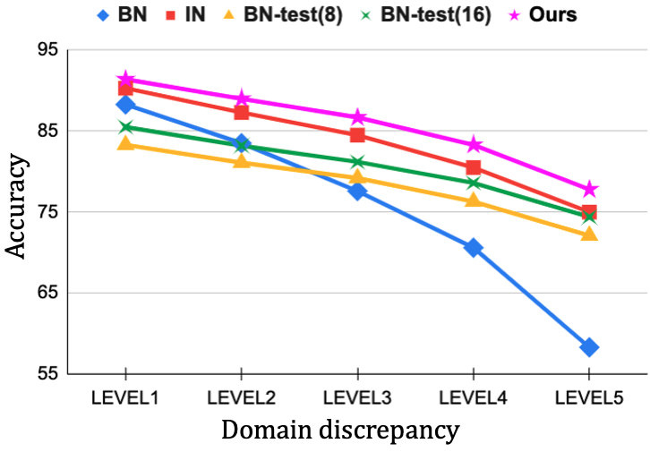
Figure 2: Accuracy of five different normalization methods for single domain generalization on CIFAR-10-C, compared at five different levels of domain discrepancy brought by corruptions. Methods include BN, IN, BN-Test (different batch sizes), and our method. See detailed experimental settings in Sec. 4.

To this end, we propose a novel adaptive form of normalization named as adaptive standardization and rescaling normalization (ASR-Norm), in which the standardization and rescaling statistics are both learned to be adaptive to each individual input sample. When being used with ADA [53, 52, 20], ASR-Norm can learn the normalization statistics by approximately optimizing a robust objective, making the statistics be adaptive to the data coming from different domains, and hence helping the model to generalize better across domains than traditional normalization approaches. We also show that ASR-Norm can be viewed as a generic form of the traditional normalization approaches including BN, IN, layer normalization (LN) [1], group normalization (GN) [55], and switchable normalization (SN) [32].

Our main contributions are as follows: (1) We propose a novel adaptive normalization, the missing ingredient for current works on ADA for single domain generalization. To the best of our knowledge, the proposed ASR-Norm is the first to learn both standardization and rescaling statistics in normalization with neural networks. (2) We show that ASR-Norm can bring consistent improvements to the state-of-the-art ADA approaches on three commonly used single domain generalization benchmarks. The performance gain is agnostic to the choice of ADA methods and becomes more significant as the domain discrepancy increases.

2 Related work

Domain Discrepancy. Domain adaptation [11, 49, 43, 59] alleviates the effect of domain discrepancy by allowing the model to see unlabeled target domain data during training. By contrast, domain generalization aims to learn domain-invariant representations so as to improve the generalization without any access to the target domains. The majorities of the literatures on domain generalization [42, 20, 6, 45, 61] focus on learning the domain invariant knowledge from multiple source domains. Another line of works studies a more challenging and realistic setting, single domain generalization, which is the focus of this paper. A few recent works on single domain generalization [53, 52, 42, 60] show that ADA can effectively improve the generalization and robustness of models by synthesizing virtual images during training. For example, Volpi et al. [53] generated the virtual images with adversarial updates on the input images while maintaining the semantic similarities with the original images. Volpi and Murino [52] proposed a random search data augmentation (RSDA) algrorithm that picks one set of the most challenging transformations in terms of inference accuracy to augment the image for training. On the other side, Huang et al. [20] proposed a representation self-challenging (RSC) algorithm to virtually augment challenging data by shutting down the dominant neurons that have the largest gradients during training. Our work builds an adaptive normalization scheme and combines it with ADA which yields a better generalization ability across domains than the state-of-the-art single domain generalization approaches.

Robustness against Distributional Shifts. Adversarial training [13, 35] aims to make models be robust to adversarial examples with imperceptible perturbations added to the inputs. However, our work focuses on the generalization ability to more perceptible and natural distributional shifts brought by the domain discrepancy. Meanwhile, there are also works trying to improve model robustness to natural and perceptible noises with pretrain [17, 15, 18], data augmentation [17, 16, 42], contrastive learning [7], stochastic networks [9, 10], etc. This setting can be included into the single domain generalization framework by viewing different distortions as different domains. Our work is compatible with these methods and can potentially further improve the performance in single domain generalization.

Normalization in Neural Networks. Since the invention of BN [22], various normalization techniques [37, 45, 23, 32, 55, 29, 54, 44, 56, 1, 50] have been proposed for different applications. Batch-instance normalization (BIN) [39] and SN [32, 46] were proposed to generalize the fixed normalizations by combining their standardization statistics with the learnable weights. However, their restrictive forms still do not allow enough adaptivity. More recently, instance-level meta (ILM) normalization [23] focused on improving the rescaling performance by using neural networks to learn the rescaling statistics. Before our work, the majorities of the works on normalization do not study the generalization ability under domain shift. Below are a few exceptions: BN-Test [37] uses testing time statistics, making its performance highly depend on the testing batch size; DSON [45] requires multi-source training data to learn separate BIN for each domain and ensemble the normalization during testing. Compared with these methods, our normalization scheme does not impose dependencies between the testing samples, requires only the single domain training data, and is generic by learning both the standardization and rescaling statistics.

3 Adversarially Adaptive Normalization

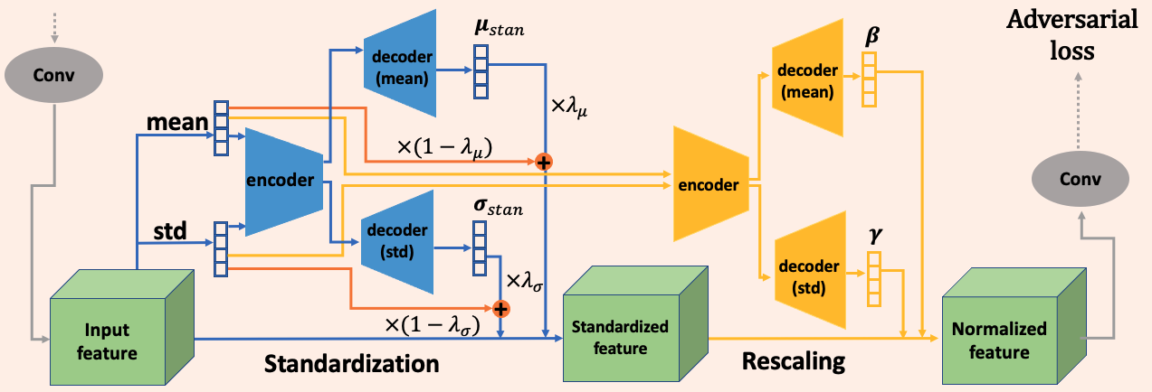
Figure 3: Illustration of the ASR-Norm layer. It can be divided into two steps: standardization and rescaling. We use encoder-decoder structured networks to learn both the standardization and rescaling statistics from the channel-wise statistics of the input. For standardization, we combine the learned statistics and native statistics with adaptive weights for stabilizing the training process.

3.1 Background

3.1.1 Single Domain Generalization Problem Setup

Consider a supervised learning problem with the training dataset $\mathcal{D}_{s}\sim P_{s}$ , where $P_{s}$ denotes the source domain distribution. The goal of single domain generalization is to train a model using single source domain data $\mathcal{D}_{s}$ to correctly classify the images from a target domain distribution $P_{t}$ unavailable during training. In this case, using the vanilla empirical risk minimization (ERM) [51] solely on the source domain ${P}_{s}$ as the training objective could be sub-optimal and yield a model that does not generalize well to unseen domains [53]. Denote $\theta$ as the model parameters and $l:\mathcal{X}\times\mathcal{Y}\rightarrow\mathbb{R}$ as the loss function. To help the model better generalize to the unseen domains, a robust objective that considers a worst-case problem around the source domain $P_{s}$ has been proposed in [47] as

$$\mathcal{L}_{R}(\theta):=\sup_{P:D(P,P_{s})\leq\rho}\mathbb{E}_{\{X,Y\}\sim P}[l(\theta;X,Y)],\vspace{-1mm}$$ (1)

where $D(P,Q)$ is a distance metric on domain distributions. The robust objective $\mathcal{L}_{R}$ enables training a model which performs well on the distributions that are $\rho$-distance away from the source domain distribution $P_{s}$. However, it is generally difficult to directly optimize the robust objective.

3.1.2 Adversarial Domain Augmentation

The optimization of $\mathcal{L}_{R}$ can be converted to a Lagrangian optimization problem with a penalty parameter $\eta$ and solved via a min-max approach:

$$\mathcal{L}_{RL}:=\sup_{P}\{\mathbb{E}_{P}[l(\theta;(X,Y))]-\eta D(P,P_{s})\}.\vspace{-1mm}$$ (2)

Defining the distance $D$ between two distributions by the Wasserstein distance [53] on a learned semantic space, the gradient of $\mathcal{L}_{RL}$, under suitable condition, can then be written as $\nabla_{\theta}L_{RL}=\mathbb{E}_{(X,Y)\sim P_{s}}[\nabla_{\theta}l(\theta;(X_{\eta}^{*},Y))],$ where $X_{\eta}^{*}:=\operatorname*{argmax}_{x\in\mathcal{X}}\{l(\theta;(x,Y))-\eta c_{\theta}((x,Y)),(X,Y))\},$ and $c_{\theta}$ is a learned distance measure over the space $\mathcal{X}\times\mathcal{Y}$ (see details in Appendix Sec. B) [53, 3]. Gradient ascent was proposed to find approximation $X_{\text{aug}}$, to $X_{\eta}^{*}$, which maximizes the prediction loss $l$ while maintaining close semantic distance to the original image $X$. The synthesized image, $X_{\text{aug}}$, with its label is then appended to the training dataset. This phase, referred to as the maximization phase, is alternated with the minimization phase, where we optimize $\theta$ to minimize the prediction loss on both the original and augmented data.

3.1.3 Standardization and Rescaling in Normalization

This section briefly introduces the normalization framework. Denote the input tensor of a normalization layer by $\boldsymbol{x}\in\mathbb{R}^{C\times H\times W}$, where $C$ denotes the number of channels of the tensor, $H$ denotes the height, and $W$ denotes the width. A typical normalization layer consists of two steps: standardization and rescaling. During standardization, the mean and standard deviation, ${\boldsymbol{\mu}}_{\text{stan}},{\boldsymbol{\sigma}}_{\text{stan}}\in\mathbb{R}^{C}$, are derived from the input tensors and used to standardize the input tensors (a small positive number, $\epsilon$, is added to ${\boldsymbol{\sigma}}_{\text{stan}}$ to avoid numerical issues). At the rescaling step, the standardized activations $\boldsymbol{x}_{\text{stan}}$ are rescaled with the rescaling statistics ${\boldsymbol{\gamma}},{\boldsymbol{\beta}}\in\mathbb{R}^{C}$:

$$\begin{cases}\boldsymbol{x}_{\text{stan}}=(\boldsymbol{x}-{\boldsymbol{\mu}}_{\text{stan}})/({\boldsymbol{\sigma}}_{\text{stan}}+\epsilon),\\ \boldsymbol{x}_{\text{norm}}=\boldsymbol{x}_{\text{stan}}*{\boldsymbol{\gamma}}+{\boldsymbol{\beta}}.\end{cases}\vspace{-1mm}$$ (3)

Different types of normalization share the similar formula but differ in the way of measuring the statistics. For example, BN computes the statistics for each batch, while IN, GN and LN compute the statistics for each sample with different channel groups. SN combines the statistics of these normalizations with learnable weights. In this work, we aim to build an adaptive normalization with statistics learned by neural networks to improve the model’s domain generalization capability.

3.2 ASR-Norm: Adaptive Standardization and Rescaling Normalization

In this section, we propose a novel generic and adaptive normalization technique, ASR-Norm, short for Adaptive Standardization and Rescaling Normalization. ASR-Norm learns both standardization and rescaling statistics with auto-encoder structured neural networks. ASR-Norm is adaptive to the individual input sample and therefore has a consistent computational graph between training and testing. Additionally, we introduce a residual term for the standardization statistics to stabilize the learning process. Using ASR-Norm with ADA can learn robust normalization statistics to enhance the model’s domain generalization ability. An overview of the proposed ASR-Norm is shown in Fig. 3 with details in the following sections.

3.2.1 Adaptive Standardization (AS)

A Functional Form. The standardization statistics can be viewed as the functions of the input tensor $\boldsymbol{x}$, i.e.,

$${\boldsymbol{\mu}}_{\text{stan}}=f(\boldsymbol{x}),{\boldsymbol{\sigma}}_{\text{stan}}=g(\boldsymbol{x}).\vspace{-1mm}$$ (4)

Remark 1.

This form generalizes a variety of normalization methods:

• If $f,g$ are constant functions with values being the statistics ${\boldsymbol{\mu}}_{0},{\boldsymbol{\sigma}}_{0}$ computed from the whole training set, this form is equivalent to BN with all training data as a batch: $f_{\text{BN}}(\boldsymbol{x})={\boldsymbol{\mu}}_{0},g_{\text{BN}}(\boldsymbol{x})={\boldsymbol{\sigma}}_{0};$

• If $f,g$ are domain-wise constant functions with values being the statistics ${\boldsymbol{\mu}}_{d},{\boldsymbol{\sigma}}_{d}$ computed for each domain $P_{d}$ in the whole training set, this form is equivalent to domain-specific BN (DSBN) with each domain data as a batch: $f_{\text{DSBN}}(\boldsymbol{x})=\sum_{d=1}^{N_{d}}{\boldsymbol{\mu}}_{d}{\bf 1}_{\{\boldsymbol{x}\in P_{d}\}},g_{\text{DSBN}}(\boldsymbol{x})=\sum_{d=1}^{N_{d}}{\boldsymbol{\sigma}}_{d}{\bf 1}_{\{\boldsymbol{x}\in P_{d}\}},$ where $N_{d}$ is the number of domains;

• If $f,g$ are the mean and std functions for each group of channels respectively, this form is equivalent to GN, which also generalizes IN and LN;

• If $f,g$ are weighted combinations of BN, IN, and LN, this form is equivalent to SN:

  $f_{\text{SN}}(\boldsymbol{x})=w_{1}f_{\text{BN}}(\boldsymbol{x})+w_{2}f_{\text{IN}}(\boldsymbol{x})+w_{3}f_{\text{LN}}(\boldsymbol{x})$,

  $g_{\text{SN}}(\boldsymbol{x})=w_{1}^{\prime}g_{\text{BN}}(\boldsymbol{x})+w_{2}^{\prime}g_{\text{IN}}(\boldsymbol{x})+w_{3}^{\prime}g_{\text{LN}}(\boldsymbol{x}).$

From the above observations, we notice that each normalization imposes a rather restrictive form of $f$ and $g$, which limits the flexibility of the normalization layers. As a result, we propose to use neural networks to fully learn the functions $f,g$ so as to provide a generic way to obtain standardization statistics.

Standardization Neural Networks. Our goal is to construct mappings from the feature map $\boldsymbol{x}$ to the learned statistics ${\boldsymbol{\mu}}_{\text{stan}}$ and ${\boldsymbol{\sigma}}_{\text{stan}}$. To lower the computational cost and leverage the original statistics information contained in the convolutional feature maps, the standardization network chooses the channel-wise mean and standard deviation statistics, instead of the original feature map, as the input to learn the standardization statistics.

Formally, denote channel-wise mean and standard deviation statistics vector of $\boldsymbol{x}$ by ${\boldsymbol{\mu}},{\boldsymbol{\sigma}}\in\mathbb{R}^{C}$, respectively. The per-channel mean and standard deviation are expressed as

$$\begin{cases}\mu_{c}=\sum_{i=1}^{H}\sum_{j=1}^{W}\boldsymbol{x}_{cij}/(H\times W),\\ \sigma_{c}=\sqrt{\sum_{i=1}^{H}\sum_{j=1}^{W}(\boldsymbol{x}_{cij}-\mu_{c})^{2}/(H\times W)}\end{cases}\vspace{-1mm}$$ (5)

for $c=1,...,C$.

We make use of an encoder-decoder structure [19, 23] to learn ${\boldsymbol{\mu}}_{\text{stan}}$ and ${\boldsymbol{\sigma}}_{\text{stan}}$ from ${\boldsymbol{\mu}}$ and ${\boldsymbol{\sigma}}$ respectively, where the encoder extracts global information by interacting the information of all channels and the decoder learns to decompose the information for each channel. For the sake of efficiency, both the encoder and decoder consist of one fully-connected layer, forming a bottleneck connected by a non-linear activation function, ReLU. Another ReLU [38] layer is applied to the output of ${\boldsymbol{\sigma}}_{\text{stan}}$ to make sure it is non-negative:

$$\begin{cases}{\boldsymbol{\mu}}_{\text{stan}}=f(\boldsymbol{x}):=f_{\text{dec}}(\text{ReLU}(f_{\text{enc}}({\boldsymbol{\mu}}))),\\ {\boldsymbol{\sigma}}_{\text{stan}}=g(\boldsymbol{x}):=\text{ReLU}(g_{\text{dec}}(\text{ReLU}(g_{\text{enc}}({\boldsymbol{\sigma}})))),\end{cases}\vspace{-1mm}$$ (6)

where $f_{\text{enc}},f_{\text{dec}},g_{\text{enc}},g_{\text{dec}}$ are fully-connected layers. The encoders project the input to the hidden space $\mathbb{R}^{C_{\text{stan}}}$, while the decoders project it back to the space $\mathbb{R}^{C}$, where $C_{\text{stan}}<C$. In practice, we find that sharing the encoders for ${\boldsymbol{\mu}}_{\text{stan}}$ and ${\boldsymbol{\sigma}}_{\text{stan}}$ would not affect the performance and save memory. Therefore, we let $f_{\text{enc}}=g_{\text{enc}}$.

Residual Learning. In the early training stage, the learning process of the standardization networks can be unstable and lead to numerical issues when the learned statistics are inaccurate. For example, ${\boldsymbol{\sigma}}_{\text{stan}}$ could be very small due to the ReLU activation, making the scale of $\boldsymbol{x}_{\text{stan}}$ very large. One remedy for this is to impose additional restrictive activation functions, such as sigmoid, on ${\boldsymbol{\sigma}}_{\text{stan}}$ so that the output values ${\boldsymbol{\sigma}}_{\text{stan}}$ are bounded. However, this could harm the training process for the case that the scale of $\boldsymbol{x}_{\text{stan}}$ is large when the scale of $\boldsymbol{x}$ is large. To retain the flexibility of ${\boldsymbol{\sigma}}_{\text{stan}}$’s scale, we stick to the ReLU activation and solve the numerical issue by introducing a residual term for regularization. In particular, we make both ${\boldsymbol{\mu}}_{\text{stan}}$ and ${\boldsymbol{\sigma}}_{\text{stan}}$ as weighted sums of the learned and original statistics:

$$\begin{cases}{\boldsymbol{\mu}}_{\text{stan}}=\lambda_{\boldsymbol{\mu}}f_{\text{dec}}(\text{ReLU}(f_{\text{enc}}({\boldsymbol{\mu}})))+(1-\lambda_{\boldsymbol{\mu}}){\boldsymbol{\mu}},\\ {\boldsymbol{\sigma}}_{\text{stan}}=\lambda_{\boldsymbol{\sigma}}\text{ReLU}(g_{\text{dec}}(\text{ReLU}(g_{\text{enc}}({\boldsymbol{\sigma}})))+(1-\lambda_{\boldsymbol{\sigma}}){\boldsymbol{\sigma}}.\end{cases}\vspace{-1mm}$$ (7)

The weights $\lambda_{\boldsymbol{\mu}},\lambda_{\boldsymbol{\sigma}}$ are learnable parameters ranging from $0$ to $1$ (bounded by sigmoid). They are both initialized with small values close to $0$ so that the standardization process is stable in the early stage and the network can gradually switch to the learned statistics in the later stage (see Fig. 5).

Remark 2.

All statistics and transformation operations in AS are computed for each sample independently. Unlike BN, AS removes the dependencies among samples during standardization. The computational graph of AS is consistent between the training and testing.

3.2.2 Adaptive Rescaling (AR)

Data-dependent rescaling parameters. Most normalization layers use the learnable parameters ${\boldsymbol{\gamma}},{\boldsymbol{\beta}}\in\mathbb{R}^{C}$ to rescale standardized output $\boldsymbol{x}_{\text{stan}}$, resulting in a rescaling process that is uniform to all samples. Recently, Jia et al. [23] found that making the rescaling parameters dependent on the samples and allowing different samples to have different rescaling parameters can bring performance gain to instance-level normalization for a variety of in-domain tasks. Inspired by this observation, we construct a rescaling network for the adaptive rescaling in ASR-Norm.

Rescaling Neural Networks. Similar to the standardization networks, we define the following network to learn the rescaling parameters from the original statistics ${\boldsymbol{\mu}},{\boldsymbol{\sigma}}$:

$$\begin{cases}{\boldsymbol{\beta}}=\psi(\boldsymbol{x}):=\text{tanh}(\psi_{\text{dec}}(\text{ReLU}(\psi_{\text{enc}}({\boldsymbol{\mu}}))))+{\boldsymbol{\beta}}_{\text{bias}},\\ {\boldsymbol{\gamma}}=\phi(\boldsymbol{x}):=\text{sigmoid}(\phi_{\text{dec}}(\text{ReLU}(\phi_{\text{enc}}({\boldsymbol{\sigma}}))))+{\boldsymbol{\gamma}}_{\text{bias}},\end{cases}\vspace{-1mm}$$ (8)

where $\phi_{\text{enc}}$, $\phi_{\text{dec}}$, $\psi_{\text{enc}}$, $\psi_{\text{dec}}$ are fully-connected layers, and sigmoid(), tanh() are activation functions to ensure the rescaling statistics are bounded. The encoders project the inputs to the hidden space $\mathbb{R}^{C_{\text{rescale}}}$ with $C_{\text{rescale}}<C$. The decoders project the encoded feature back to the space $\mathbb{R}^{C}$. ${\boldsymbol{\gamma}}_{\text{bias}},{\boldsymbol{\beta}}_{\text{bias}}\in\mathbb{R}^{C}$ are learned parameters and are initialized with ones and zeros, respectively, as the traditional rescaling parameters. The encoders for ${\boldsymbol{\beta}},{\boldsymbol{\gamma}}$ are also shared according to the same reason as the standardization networks, i.e., $\phi_{\text{enc}}=\psi_{\text{enc}}$.

3.2.3 Adversarially Adaptive Normalization

The parameters in ASR-Norm can be learned together with the model $\theta$ by the robust objective as $\theta$ in Eq 2. With ADA, the objective can be optimized approximately, and ASR-Norm can learn the normalization statistics to be adaptive to the data coming from different domains, thus helping the model generalize well across domains. Note that the proposed normalization is agnostic to the choice of ADA. In the experiments, we show the implementations and performances of our method coupling with three different ADA methods.

4 Experiments

4.1 Experimental Settings

Datasets. We conduct experiments on three standard benchmarks for single domain generalization [53, 52, 60, 42], including Digits, CIFAR-10-C, and PACS.

(1) Digits: This benchmark consists of five digits datasets: MNIST [27], SVHN [40], MNIST-M [11], SYN [11], and USPS [21] (see examples in Fig. 9 in Appendix). We use MNIST as the source domain, and the rest as the target domains. All images are resized to $32\times 32$ pixels and the channels of MNIST and USPS are duplicated so that different datasets have compatible shapes.

(2) CIFAR-10-C [14]: This benchmark is proposed to evaluate the robustness to $19$ types of corruptions with $5$ levels of intensities. The original CIFAR-10 [26] is used for training and corruptions are only applied to the testing images (see examples in Fig. 4). The level of domain discrepancy can be measured by the corruption intensity.

Figure 4: Example images with level $5$ corruption from $4$ corruption types in the CIFAR-10-C benchmark.

(3) PACS [30]: A recent benchmark for domain generalization containing four domains: art paint, cartoon, sketch, and photo (see examples in Fig. 1). This dataset is considered to pose a challenging distributional shift for domain generalization. For this dataset, we consider two settings: 1) training a model with one domain data and testing with the rest three domains; 2) training a model on three domains and test on the remaining one. The second setting is widely used for multi-source domain generalization with the domain label available for training. In our experiment for single domain generalization, we remove the domain label and mix data from multiple source domains during training.

Implementation Details. For ASR-Norm, unless otherwise noted, $C_{\text{stan}},C_{\text{rescale}}$ are set to $C/2,C/16$, respectively, and $\lambda_{\boldsymbol{\mu}},\lambda_{\boldsymbol{\sigma}}$ are both initialized as sigmoid(-3).

(1) For Digits, we use the ConvNet architecture [27] (conv-pool-conv-pool-fc-fc-softmax) with ReLU following each convolution. Since this model does not have any normalization layer, ASR-Norm is inserted after each conv layer before ReLU. We adopt RSDA [52] for domain augmentation, which is the state-of-the-art (SOTA) on this benchmark, and follow its experimental settings: setting the size of transformation tuples as $3$, using a subset of $1,000$ samples from training set to select the worst transformation, conducting the search every $1,000$ steps, running a total of $10^{6}$ weight updates, and using Adam [24] optimizer with learning rate $10^{-4}$ and mini-batch size $32$.

(2) For CIFAR-10-C, we use the Wide Residual Network (WRN) [58] with $40$ layers and widen factor $4$. We follow the experiment setting in [58] to use SGD with Nesterov momentum ($0.9$) and batch size $128$. The learning rate starts at $0.1$ with cosine annealing [31]. Models are trained for $200$ epochs in total. We replace the default BN with ASR-Norm and train with ADA [53], where the augmentation is performed for every $1000$ steps of training with three augmentations in total, and each augmentation step consists of $25$ gradient updates.

(3) For PACS, we use a ResNet-18 pretrained on ImageNet as the backbone and add a fully-connected layer for classification as the setting in [20] which presented the SOTA domain generalization performance on PACS. The BN in the ResNet-18 model is substituted by ASR-Norm. We find that directly replacing BN with ASR-Norm during the fine tuning stage fails to work. The main reason is that the models are sensitive to the scale of the activations after pretrain and replacing the rescaling parameters with the AR networks could lead to significant changes in the activation scales. To remedy the issue, we resume ${\boldsymbol{\beta}}_{\text{bias}}$ and ${\boldsymbol{\gamma}}_{\text{bias}}$ from the BN layers in the pretrained model and add learnable weights $\lambda_{\boldsymbol{\beta}},\lambda_{\boldsymbol{\gamma}}$ to the first terms:

$$\begin{cases}{\boldsymbol{\beta}}=\psi(\boldsymbol{x})=\lambda_{\boldsymbol{\beta}}\text{tanh}(\psi_{\text{dec}}(\text{ReLU}(\psi_{\text{enc}}({\boldsymbol{\mu}}))))+{\boldsymbol{\beta}}_{\text{bias}},\\ {\boldsymbol{\gamma}}=\phi(\boldsymbol{x})=\lambda_{\boldsymbol{\gamma}}\text{sigmoid}(\phi_{\text{dec}}(\text{ReLU}(\phi_{\text{enc}}({\boldsymbol{\sigma}}))))+{\boldsymbol{\gamma}}_{\text{bias}},\end{cases}\vspace{-1mm}$$ (9)

where we initialize $\lambda_{\boldsymbol{\beta}}$ and $\lambda_{\boldsymbol{\gamma}}$ with a small value, $\text{sigmoid}(-5)$, to smooth the learning process. In this way, the scale of $\boldsymbol{x}_{\text{norm}}$ will be close to that of the pretrained models initially. The network can gradually learn to make use of the learned statistics. During training, the model learns ASR-Norm with the RSC procedure [20] by SGD optimizer with the initial learning rate as $0.004$, which decays to $10\%$ after 24 epochs. Models are trained for $30$ epochs with the batch size of $128$.

4.2 Main Results: Comparing with the SOTA

Our approach improves upon the SOTA single domain generalization results by $1.6\%$, $2.7\%$, and $6.3\%$ on the Digits, CIFAR-10-C, and PACS benchmarks, respectively.

Method	SVHN	MNIST-M	SYN	USPS	Avg.
ERM	27.8	52.7	39.7	76.9	49.3
CCSA[36]	25.9	49.3	37.3	83.7	49.1
d-SNE[57]	26.2	51.0	37.8	93.2	52.1
JiGen[5]	33.8	57.8	43.8	77.2	53.1
ADA[53]	35.5	60.4	45.3	77.3	54.6
M-ADA[42]	42.6	67.9	49.0	78.5	59.5
ME-ADA[60]	42.6	63.3	50.4	81.0	59.3
RSDA[52]	47.4$\pm$4.8	81.5$\pm$1.6	62.0$\pm$1.2	83.1$\pm$1.2	68.5
RSDA+ASR (Ours)	52.8$\pm$3.8	80.8$\pm$0.6	64.5$\pm$1.1	82.4$\pm$1.4	70.1
$\Delta$ to RSDA	5.4	-0.7	2.5	-0.7	1.6

Table 1: Single domain generalization accuracies on Digits. MNIST is used as the training set, and the results on different testing domains are reported in different columns.

Results on Digits. Table 1 shows the results on the Digits benchmark. The proposed method, ASR-Norm, is combined with RSDA and compared with methods including: (1) ERM which uses cross-entropy loss for training, without domain augmentation; (2) CCSA [36] which regularizes latent features to improve generalization; (3) d-SNE [57] which uses stochastic neighborhood embedding techniques and a novel modified-Hausdorff distance for training; (4) JiGen [5] which adds the patch order prediction as auxiliary; (5) ADA [53]; (6) M-ADA [53] which uses Wasserstein auto-encoder and meta-learning to improve ADA; (7) ME-ADA [60] which adds entropy regularization to help ADA; (8) RSDA [52] which does not use normalization. Our method outperforms both the baseline and the SOTA methods on average. In particular, our method improves the performance on challenging domains like SVHN and SYN. We have similar observations on USPS as [42], where ADA-based methods are not as good as CCSA or d-SNE due to USPS’s strong similarity with MNIST (see Fig. 9).

Method	Level 1	Level 2	Level 3	Level 4	Level 5	Avg.
ERM	87.8$\pm$0.1	81.5$\pm$0.2	75.5$\pm$0.4	68.2$\pm$0.6	56.1$\pm$0.8	73.8
PGD[34]	73.1$\pm$0.5	69.0$\pm$1.1	64.1$\pm$1.3	58.0$\pm$2.2	48.9$\pm$2.8	61.6
ST [15]	-	-	-	-	-	76.9
TTT [48]	-	-	-	-	-	84.4
ADA[53]	88.3$\pm$0.6	83.5$\pm$2.0	77.6$\pm$2.2	70.6$\pm$2.3	58.3$\pm$2.5	75.7
M-ADA[42]	90.5$\pm$0.3	86.8$\pm$0.4	82.5$\pm$0.6	76.4$\pm$0.9	65.6$\pm$1.2	80.4
ME-ADA[60]	-	-	-	-	-	83.3
ERM+ASR	89.4$\pm$0.2	86.1$\pm$0.2	82.9$\pm$0.3	78.6$\pm$0.6	72.9$\pm$1.0	82.0
ADA+ASR (Ours)	91.5$\pm$0.2	89.3$\pm$0.6	86.9$\pm$0.5	83.7$\pm$0.7	78.4$\pm$0.8	86.0
$\Delta$ to ADA	3.2	5.8	9.3	13.1	20.1	10.3

Table 2: Single domain generalization accuracies on CIFAR-10. CIFAR-10 is used as the training domain, while CIFAR-10-C with different corruption types and corruption levels are used as the testing domains.

Results on CIFAR-10-C. We report the average accuracies of the $19$ corruption types for each level of intensity on CIFAR-10-C in Table 2 (we also provide results for each corruption type in Fig. 6 in Appendix Sec. A). ERM, ADA[53], M-ADA[52], ME-ADA[60], ST[15], and TTT[48] are used for the comparison on this benchmark. We also include the results by using project gradient descent (PGD) [34] for adversarial training. The results show ASR-Norm makes significant improvement over ADA and all other improved ADA-based methods such as M-ADA and ME-ADA, as well as self-supervised method ST and test-time training method TTT. Similar to the results on the Digits benchmark, ASR-Norm achieves larger improvements on the more challenging domains, i.e., domains with more intense corruptions, than on the less challenging ones. We also note that the standard PGD training for defending against adversarial examples does not help improve robustness to perceivable noises in this dataset.

Method	Artpaint	Cartoon	Sketch	Photo	Avg.
ERM	70.9	76.5	53.1	42.2	60.7
RSC[20]	73.4	75.9	56.2	41.6	61.8
RSC+ASR (Ours)	76.7	79.3	61.6	54.6	68.1
$\Delta$ to RSC	3.3	3.4	5.4	13.0	6.3

Table 3: Single domain generalization accuracies on PACS. One domain (name in column) is used as the training set and the other domains are used as the testing set.

Results on PACS. In Table 3, we show the results on PACS where we use one domain for training and the rest three for testing. The reported numbers are the average accuracies across the testing domains. Again, ASR-Norm improves the performance of RSC significantly, especially on challenging domains. Table 4 shows the results on PACS for the multi-source domain setting, where we do not utilize domain labels during training. Similarly, ASR-Norm outperforms not only the SOTA performance reported by RSC but also the other SOTA methods, including those that make use of the domain labels, such as DSON and MetaReg.

Method	Artpaint	Cartoon	Sketch	Photo	Avg.
ERM	79.0	73.9	70.6	96.3	79.9
JiGen[5]	79.4	75.3	71.4	96.0	80.5
MetaReg [2]	83.7	77.2	70.3	95.5	81.7
Cutout[8]	79.6	75.4	71.6	95.9	80.6
DropBlock[12]	80.3	77.5	76.4	95.6	82.5
AdversarialDropout[41]	82.4	78.2	75.9	91.1	83.1
BIN[45]	82.1	74.1	80.0	95.0	82.8
SN[32]	78.6	75.2	77.4	91.1	80.6
DSON[45]	84.7	77.7	82.2	95.9	85.1
RSC[20]	83.4	80.3	80.9	96.0	85.2
RSC+ASR (Ours)	84.8	81.8	82.6	96.1	86.3
$\Delta$ to RSC	1.4	1.5	1.7	0.1	1.1

Table 4: Domain generalization accuracies on PACS. One domain (name in column) is used as the test set and the other domains are used as the training sets. During training, no domain identification is used.

4.3 Result Analysis

On the Effect of Normalization. In Table 5, we study the effect of using different normalizations on the generalization ability for CIFAR-10-C benchmark (Table 9 in Appendix reports the results on Digits). We observe that BN underperforms all the other normalization methods that have a consistent computational graph between training and testing. For this reason, our experiment with SN only includes IN and LN, but excludes BN. With the generic form that allows the model to adapt to single domain generalization easily, ASR-Norm outperforms BN, SN, and IN. The performance gain improves with the corruption level increasing. We also note that both AR and AS play a significant role in the performance gain, meaning learning both standardization and rescaling statistics in normalization is indeed helping models to learn to generalize. Further, AS achieves better performance than SN, which implies that learning only the combination weights for different standardization statistics are not as good as learning the statistics with neural networks.

Method	Level 1	Level 2	Level 3	Level 4	Level 5	Avg.
ADA+BN[53]	88.3	83.5	77.6	70.6	58.3	75.7
ADA+IN[50]	90.3	87.3	84.5	80.5	75.0	83.5
ADA+SN[32]	91.5	88.4	85.5	81.2	75.3	84.4
ADA+AR	90.4	87.7	85.1	81.1	76.6	84.2
ADA+AS	91.4	88.9	86.3	82.8	77.3	85.4
ADA+ASR (Ours)	91.5	89.3	86.9	83.7	78.4	86.0

Table 5: Single domain generalization accuracies on CIFAR-10-C with different normalizations.

Uncertainty Evaluation. For CIFAR-10-C, we also evaluate the quality of predictive probabilities using Brier score (BS) [4], defined as the squared distance between the predictive distribution and the one-hot target labels: $BS=\sum_{k=1}^{K}(1_{\{k=Y\}}-p_{\theta}(Y=k|X))^{2}/K$, where $K$ is the number of classes, and $p_{\theta}$ is the predictive probability. Table 6 shows that ASR-Norm outperforms BN and IN in uncertainty prediction, meaning that ASR-Norm provides not only better predictions for classes but also better predictive distributions. The improvement is also increasing along with the rise of the domain discrepancy.

Method	Level 1	Level 2	Level 3	Level 4	Level 5	Avg.
ADA+BN[53]	0.019	0.028	0.035	0.044	0.061	0.037
ADA+IN[50]	0.015	0.020	0.025	0.032	0.041	0.027
ADA+ASR (Ours)	0.014	0.018	0.022	0.027	0.037	0.024
$\Delta$ to BN	-0.005	-0.010	-0.013	-0.017	-0.024	-0.013

Table 6: Uncertainty evaluations of different normalizations at different corruption levels using Brier score (the smaller the better) on CIFAR-10-C.

In-domain Performance and Adversarial Robustness. In Table 7, we report the in-domain performance of different normalizations by evaluating on the original CIFAR-10 testing set without corruptions. We note that BN indeed achieves better performance than IN and ASR-Norm on in-domain data. One explanation for that is the dependencies between training samples introduces the inductive biases that would help BN when samples come from the same domain. We also test the robustness towards adversarial attacks of each normalization, where we first apply several adversarial updates on each testing image and then make predictions on the adversarially corrupted image. The results in Table 7 show that ASR-Norm benefits from its adaptation capability and achieves better performance under adversarial attack.

Domain	ADA+BN	ADA+IN	ADA+ASR (Ours)
In-domain	95.4	94.6	94.6
Adversarial	32.0	46.9	52.2

Table 7: Evaluation of different normalizations for in-domain data and adversarially corrupted images.

Analysis of Residual Learning. In our experiments, we find that the residual learning is necessary for stabilizing the training of ASR-Norm. Without this part, ASR-Norm would have numerical instabilities and yield NAN. Fig. 5 shows the evolution of the adaptive weights $\lambda_{\boldsymbol{\mu}}$ and $\lambda_{\boldsymbol{\sigma}}$ in the residual terms along the training process of the CIFAR-10-C benchmark. The weights for learned statistics are initialized close to 0 and learn to increase gradually, meaning that the model favors the learned statistics more and more, which verifies that learned statistics are indeed helping the model. Interestingly, at the end of training, $\lambda_{\boldsymbol{\sigma}}$ adapts to almost $1$, i.e., the normalization learns to use only learned ${\boldsymbol{\sigma}}_{\text{stan}}$ (see more plots on PACS in Fig. 7 in Appendix.)

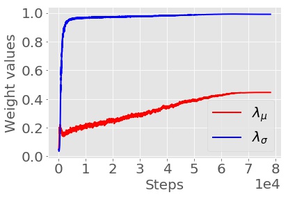
Figure 5: Weights $\lambda_{\boldsymbol{\mu}}$, $\lambda_{\boldsymbol{\sigma}}$ learn to increase along the training process for the first normalization layer in WRN on CIFAR-10-C.

Trade-off between Complexity and Performance. The complexity and performance of ASR-Norm are impacted by the number of ASR-Norm layers used and the hidden dimension sizes, $C_{\text{stan}}$ and $C_{\text{rescale}}$. As in [23], we fix $C_{\text{rescale}}$ to $16$. We conduct ablation study on PACS with the ResNet-18 backbone, shown in Table 8, to investigate the trade-off between complexity and performance by varying both the number of ASR-Norm layers applied and $C_{\text{stan}}$. First, we observe that a single layer of ASR-Norm improves over the baseline with only $0.1\%$ increase in parameters. As the number of ASR-Norm layers increases, the performance improves further at the expense of higher complexity. Second, applying ASR-Norm to all normalization layers with $C_{\text{stan}}=C/16$ could provide a significant performance boost over baseline with a small memory addition ($4.1\%$). Average accuracy increases as $C_{\text{stan}}$ increases with a sub-linear speed while parameters increase linearly with $C_{\text{stan}}$.

Norm layers ($C_{\text{stan}}$, $C_{\text{rescale}}$)	Avg.	# Params	Params $\uparrow$
BN	61.8	11.18M	0
ASR to the first norm layer ($C/2,C/16$)	62.3	11.19M	0.1%
ASR to selected 4 norm layers ($C/2,C/16$)	64.4	11.80M	5.5%
ASR to all norm layers ($C/16,C/16$)	66.5	11.64M	4.1%
ASR to all norm layers ($C/8,C/16$)	67.5	11.83M	5.8%
ASR to all norm layers ($C/2,C/16$)	68.1	13.01M	16.4%

Table 8: Trade-off between model complexity and accuracies on PACS. One domain is used for training. Average accuracies, parameter sizes, and the increasing proportion of parameter sizes with respect to the baseline are reported.

5 Conclusion

We propose ASR-Norm, a novel adaptive and general form of normalization which learns both the standardization and rescaling statistics with auto-encoder structured neural networks. ASR-Norm is a generic algorithm that complements a variety of adversarial domain augmentation (ADA) approaches on single domain generalization by making the statistics be adaptive to the data of different domains, and hence improves the model generalization capability across domains. On three standard benchmarks, we show that ASR-Norm brings consistent improvement to the state-of-the-art ADA approaches. The performance gain is agnostic to the choice of ADA methods and becomes more significant as the domain discrepancy increases.

Acknowledgements. X. Fan and M. Zhou acknowledge the support of NSF IIS-1812699 and Texas Advanced Computing Center.

Appendices for “Adversarially Adaptive Normalization for Single Domain Generalization”

Appendix A Additional Experimental Results

On the Effect of Normalization. In Table 9, we study the impact on the generalization ability by using different normalization techniques with RSDA [53] for domain augmentation on the Digits benchmark. It reports average accuracies, standard deviations and $p$-values for each domain in the Digits benchmark. We observe that adding either batch normalization (BN) or BN-test to the ConvNet architecture makes the performance worse than the baseline without any normalization layer. Instance normalization shows small improvement over the baseline but still underperforms ASR-Norm. ASR-Norm outperforms all methods on average and achieves significant improvement for challenging domains, including SVHN and SYN. On the easier domains like MNIST-M and USPS, ASR performs on a par with the baseline (RSDA).

Method	SVHN	MNIST-M	SYN	USPS	Avg.
RSDA+BN[22]	39.4$\pm$5.2	76.6$\pm$2.2	60.5$\pm$1.5	84.2$\pm$2.1	65.2
RSDA+BN-Test[37]	45.7$\pm$2.8	80.3$\pm$1.2	59.7$\pm$1.4	81.8$\pm$1.1	66.9
RSDA+IN[50]	47.1$\pm$3.4	80.6$\pm$0.9	61.9$\pm$1.5	85.4$\pm$1.4	68.8
RSDA+SN[32]	37.7$\pm$3.8	77.1$\pm$1.4	60.5$\pm$1.8	86.1$\pm$1.7	65.4
RSDA	47.4$\pm$4.8	81.5$\pm$1.6	62.0$\pm$1.2	83.1$\pm$1.2	68.5
RSDA+AR	47.8 $\pm$3.2	80.0$\pm$1.0	64.0$\pm$0.9	86.7$\pm$1.5	69.6
RSDA+AS	49.4$\pm$2.3	81.4$\pm$0.7	63.5$\pm$1.2	81.4$\pm$1.1	69.3
RSDA+ASR (Ours)	52.8$\pm$3.8	80.8$\pm$0.6	64.5$\pm$1.1	82.4$\pm$1.4	70.1
$p$-value: Ours vs. RSDA	0.036	0.193	0.003	0.197	-
$p$-value: Ours vs. AS	0.050	0.088	0.115	0.108	-
$p$-value: Ours vs. AR	0.020	0.080	0.214	$\mathbf{<1e\scalebox{0.5}[1.0]{$-$}3}$	-

Table 9: Single domain generalization accuracies with different normalization on Digits. MNIST is used as the training set, and the results on different testing domains are reported in different columns.

Statistical significance of results on CIFAR-10-C. In Table 10 reports the standard deviations and $p$-values for the one-sided two-sample $t$-test on the accuracies for CIFAR-10-C in addition to Table 5. The results show consistently statistical significance of ASR-norm’s improvements over M-ADA, SN, AR, and AS in different corruption levels.

Method	Level 1	Level 2	Level 3	Level 4	Level 5	Avg.
ERM+BN	87.8$\pm$0.1	81.5$\pm$0.2	75.5$\pm$0.4	68.2$\pm$0.6	56.1$\pm$0.8	73.8
ERM+ASR (ASR alone)	89.4$\pm$0.2	86.1$\pm$0.2	82.9$\pm$0.3	78.6$\pm$0.6	72.9$\pm$1.0	82.0
M-ADA	90.5$\pm$0.3	86.8$\pm$0.4	82.5$\pm$0.6	76.4$\pm$0.9	65.6$\pm$1.2	80.4
ADA+SN	91.5$\pm$0.2	88.4$\pm$0.6	85.5$\pm$0.5	81.2$\pm$0 7	75.3$\pm$0.8	84.4
ADA+AR	90.4$\pm$0.1	87.7$\pm$0.3	85.1$\pm$0.6	81.1$\pm$0.7	76.6$\pm$1.0	84.2
ADA+AS	91.4$\pm$0.1	88.9$\pm$0.2	86.3$\pm$0.4	82.8$\pm$0.5	77.3$\pm$0.7	85.4
ADA+ASR (Ours)	91.5$\pm$0.2	89.3$\pm$0.6	86.9$\pm$0.5	83.7$\pm$0.7	78.4$\pm$0.8	86.0
$p$-value: Ours vs. ERM/ERM+ASR/M-ADA	$\mathbf{<1e\scalebox{0.5}[1.0]{$-$}3}$	$\mathbf{<1e\scalebox{0.5}[1.0]{$-$}3}$	$\mathbf{<1e\scalebox{0.5}[1.0]{$-$}3}$	$\mathbf{<1e\scalebox{0.5}[1.0]{$-$}3}$	$\mathbf{<1e\scalebox{0.5}[1.0]{$-$}3}$	-
$p$-value: Ours vs. ADA+SN	0.5	$\mathbf{0.025}$	$\mathbf{0.006}$	$\mathbf{0.001}$	$\mathbf{<1e\scalebox{0.5}[1.0]{$-$}3}$	-
$p$-value: Ours vs. ADA+AR	$\mathbf{0.001}$	$\mathbf{0.003}$	$\mathbf{0.005}$	$\mathbf{0.003}$	$\mathbf{0.050}$	-
$p$-value: Ours vs. ADA+AS	${0.199}$	${0.121}$	$\mathbf{0.049}$	$\mathbf{0.035}$	$\mathbf{0.036}$	-

Table 10: Single domain generalization accuracies and $p$-values on CIFAR-10-C with different corruption levels. Significant results are highlighted ($p$-value $\leq 0.05$).

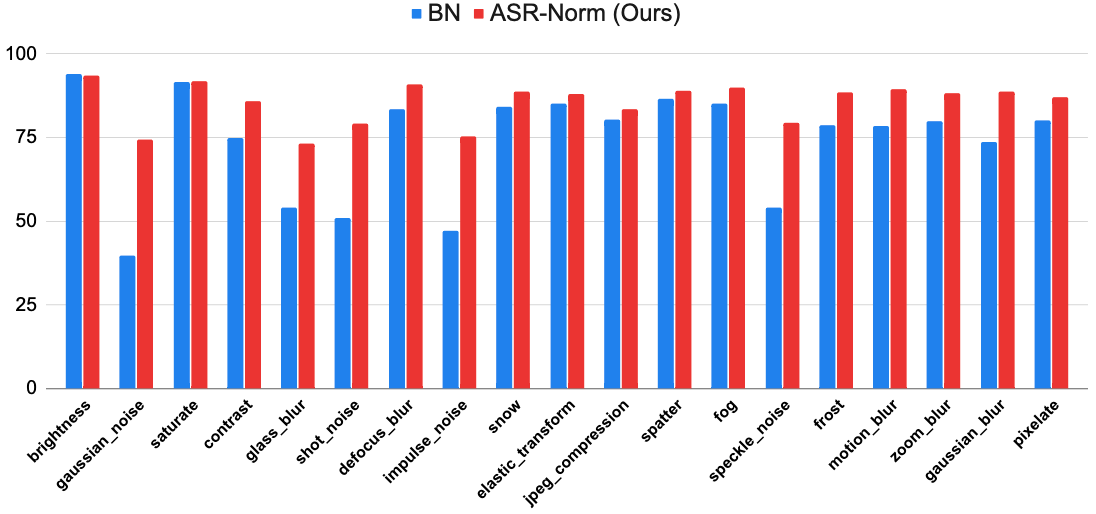
Figure 6: Single domain generalization results on CIFAR-10-C for each corruption type.

Analysis of Residual Learning. Fig. 7(a) shows the evolution of the adaptive weights $\lambda_{\boldsymbol{\mu}}$ and $\lambda_{\boldsymbol{\sigma}}$ in the residual terms of standardization statistics along the training process of the PACS benchmark. The weights for learned statistics are initialized close to 0 and learn to increase gradually, meaning that the model favors the learned statistics increasingly along the training process. That verifies the learned statistics are indeed favored the model for domain generalization. We note that the increasing speed of the residual weights for PACS is not as fast as that for CIFAR-10-C. The reason for that could be we used a pretrained model for PACS, which already learned some useful statistics. Fig. 7(b) shows the evolution of the adaptive weights $\lambda_{\beta}$ and $\lambda_{\gamma}$ in the residual terms of rescaling statistics, where we have the similar observations.

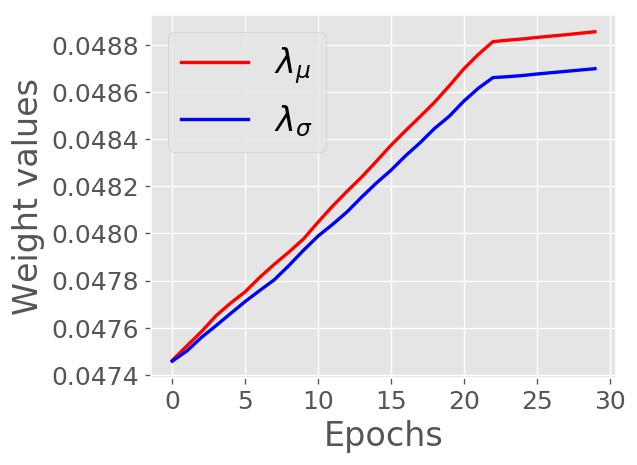
(a) Weights $\lambda_{\boldsymbol{\mu}},\lambda_{\boldsymbol{\sigma}}$.

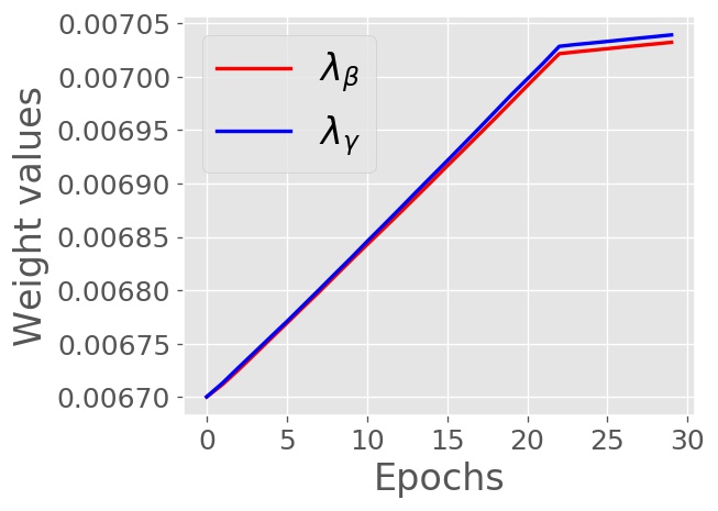
(b) Weights $\lambda_{\beta},\lambda_{\gamma}$.

Figure 7: Weights learn to increase the contribution from learned statistics along the training process on the PACS benchmark.

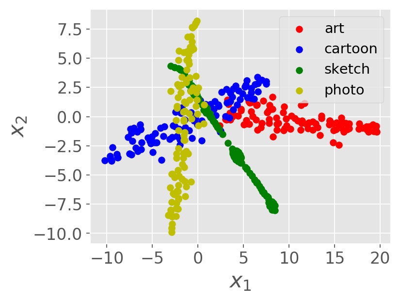
(a) Visualization of ${\boldsymbol{\sigma}}_{\text{stan}}$.

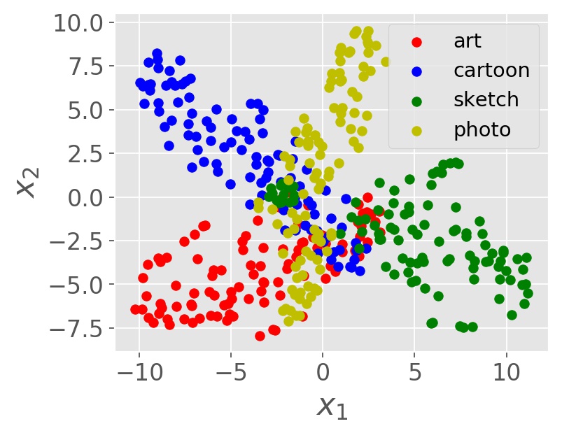
(b) Visualization of ${\boldsymbol{\mu}}_{\text{stan}}$.

Figure 8: Visualization of learned standardization statistics for different domains on PACS benchmark.

Visualization of Learned Statistics. Figure 8 visualizes the learned standardization statistics ${\boldsymbol{\mu}}_{\text{stan}}$ and ${\boldsymbol{\sigma}}_{\text{stan}}$ using t-SNE [33] for different domains in PACS. We notice that the learned statistics show clustering structures for each domain, meaning that ASR-Norm learns different patterns of standardization statistics for each domain. This finding resembles previous papers on using domain-specific statistics for multi-domain data [45]. However, our method learns the soft clustered embeddings in an automatic way without the hard domain label on each sample.

CIFAR-10-C Results for Different Corruption Types. CIFAR-10-C contains $19$ corruption types including, brightness, gaussian noise, saturate, contrast, glass blur, shot noise, defocus blur, impulse noise, snow, elastic transform, jpeg compression, spatter, fog, speckle noise, frost, motion blur, zoom blur, gaussian blur, and pixelate. These $19$ corruption types can be categoried into $4$ categories including, noise, blur, weather, and digital categories [14]. Figure 6 shows the average accuracies for each corruption type across five intensity levels. We observe that ASR-Norm makes consistent improvements over BN in most corruption types, except for brightness.

Appendix B Detailed Formulation of Adversarial Domain Augmentation

Adversarial domain augmentation (ADA) [53] approximately optimizes the robust objective $\mathcal{L}_{RL}$ in Eq 2 by expanding the training set with synthesized adversarial examples along the training process. Specifically, we define the distance $D$ between two distributions $P$ and $Q$ by the Wasserstein distance as [53]:

$$D_{\theta}(P,Q):=\inf_{M\in\Pi(P,Q)}\mathbb{E}_{M}[c_{\theta}((X,Y),(X^{\prime},Y^{\prime}))],$$ (10)

where $c_{\theta}$ is a learned distance measure over the space $\mathcal{X}\times\mathcal{Y}$. In ADA, $c_{\theta}$ is measured with the semantic features learned by the neural networks:

$$c_{\theta}((x,y),(x^{\prime},y^{\prime})):=c((F_{\theta}(x),y),(F_{\theta}(x^{\prime}),y^{\prime})),$$ (11)

where $F_{\theta}$ is a feature extractor outputting intermediate activations in the neural networks, and

$$c((z,y),(z^{\prime},y^{\prime})):=\frac{1}{2}\left\lVert z-z^{\prime}\right\rVert_{2}^{2}+\infty\cdot 1_{\{y\neq y^{\prime}\}}.$$ (12)

Then, the key observation is that optimizing $\mathcal{L}_{R}$ can be solved by optimizing the Lagrangian relaxation with penalty parameter $\eta$:

$$\mathcal{L}_{RL}:=\sup_{P}\{\mathbb{E}_{P}[l(\theta;(X,Y))]-\eta D_{\theta}(P,P_{s})\}.$$ (13)

The gradient of $\mathcal{L}_{RL}$, under a suitable condition, can be rewritten as [53, 3],

$$\nabla_{\theta}L_{RL}=\mathbb{E}_{(X,Y)\sim P_{s}}[\nabla_{\theta}l(\theta;(x_{\eta}^{*},Y))],$$ (14)

where

$$x_{\eta}^{*}=\operatorname*{argmax}_{x\in\mathcal{X}}\{l(\theta;(x,Y))-\eta c_{\theta}((x,Y)),(X,Y))\}.$$ (15)

A min-max algorithm is used to estimate the gradients approximately as discussed in Sec. 3.1.2.

Appendix C Additional Experimental Settings

In Figure 9, we show some visual examples from the Digits benchmark. SVHN, MNIST-M and SYN are more challenging domains that have larger distributional shift from MNIST than USPS.

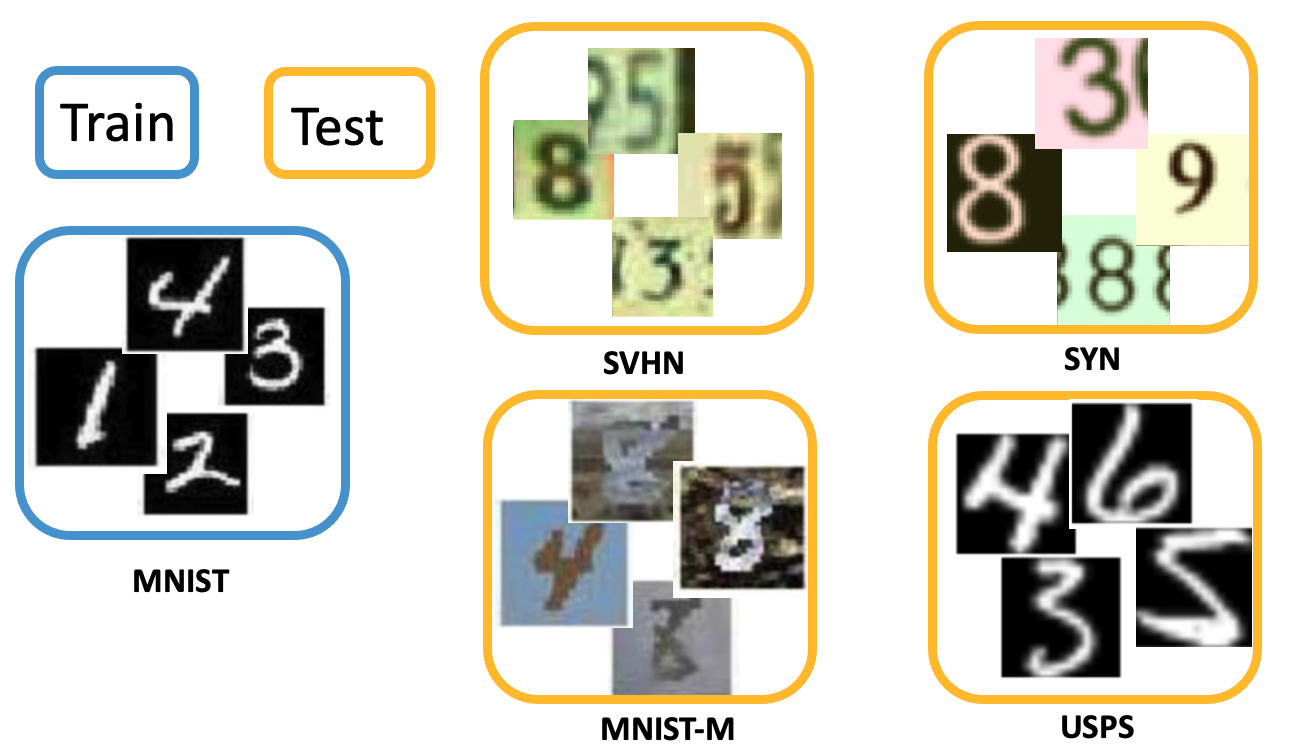
Figure 9: Single domain generalization with Digits benchmark. Only MNIST is used for training and the goal is to learn a model that generalizes well to other digits domains, including, SVHN, MNIST-M, SYN, USPS.

References

- Ba et al. [2016] J. L. Ba, J. R. Kiros, and G. E. Hinton. Layer normalization. arXiv preprint arXiv:1607.06450, 2016.
- Balaji et al. [2018] Y. Balaji, S. Sankaranarayanan, and R. Chellappa. Metareg: Towards domain generalization using meta-regularization. In Advances in Neural Information Processing Systems, pages 998–1008, 2018.
- Boyd et al. [2004] S. Boyd, S. P. Boyd, and L. Vandenberghe. Convex optimization. Cambridge university press, 2004.
- Brier [1950] G. W. Brier. Verification of forecasts expressed in terms of probability. Monthly weather review, 78(1):1–3, 1950.
- Carlucci et al. [2019] F. M. Carlucci, A. D’Innocente, S. Bucci, B. Caputo, and T. Tommasi. Domain generalization by solving jigsaw puzzles. In Proceedings of the IEEE Conference on Computer Vision and Pattern Recognition, pages 2229–2238, 2019.
- Chattopadhyay et al. [2020] P. Chattopadhyay, Y. Balaji, and J. Hoffman. Learning to balance specificity and invariance for in and out of domain generalization. ECCV, 2020.
- Chen et al. [2020] T. Chen, S. Kornblith, K. Swersky, M. Norouzi, and G. Hinton. Big self-supervised models are strong semi-supervised learners. arXiv e-prints, pages arXiv–2006, 2020.
- DeVries and Taylor [2017] T. DeVries and G. W. Taylor. Improved regularization of convolutional neural networks with cutout. arXiv preprint arXiv:1708.04552, 2017.
- Fan et al. [2020] X. Fan, S. Zhang, B. Chen, and M. Zhou. Bayesian attention modules. In Advances in Neural Information Processing Systems, volume 33, pages 16362–16376, 2020.
- Fan et al. [2021] X. Fan, S. Zhang, K. Tanwisuth, X. Qian, and M. Zhou. Contextual dropout: An efficient sample-dependent dropout module. In International Conference on Learning Representations, 2021.
- Ganin and Lempitsky [2015] Y. Ganin and V. Lempitsky. Unsupervised domain adaptation by backpropagation. In International conference on machine learning, pages 1180–1189. PMLR, 2015.
- Ghiasi et al. [2018] G. Ghiasi, T.-Y. Lin, and Q. V. Le. Dropblock: A regularization method for convolutional networks. In Advances in Neural Information Processing Systems, pages 10727–10737, 2018.
- Goodfellow et al. [2014] I. J. Goodfellow, J. Shlens, and C. Szegedy. Explaining and harnessing adversarial examples. arXiv preprint arXiv:1412.6572, 2014.
- Hendrycks and Dietterich [2018] D. Hendrycks and T. Dietterich. Benchmarking neural network robustness to common corruptions and perturbations. In International Conference on Learning Representations, 2018.
- Hendrycks et al. [2019a] D. Hendrycks, M. Mazeika, S. Kadavath, and D. Song. Using self-supervised learning can improve model robustness and uncertainty. In Advances in Neural Information Processing Systems, pages 15663–15674, 2019a.
- Hendrycks et al. [2019b] D. Hendrycks, N. Mu, E. D. Cubuk, B. Zoph, J. Gilmer, and B. Lakshminarayanan. Augmix: A simple data processing method to improve robustness and uncertainty. In International Conference on Learning Representations, 2019b.
- Hendrycks et al. [2020a] D. Hendrycks, S. Basart, N. Mu, S. Kadavath, F. Wang, E. Dorundo, R. Desai, T. Zhu, S. Parajuli, M. Guo, et al. The many faces of robustness: A critical analysis of out-of-distribution generalization. arXiv preprint arXiv:2006.16241, 2020a.
- Hendrycks et al. [2020b] D. Hendrycks, X. Liu, E. Wallace, A. Dziedzic, R. Krishnan, and D. Song. Pretrained transformers improve out-of-distribution robustness. arXiv preprint arXiv:2004.06100, 2020b.
- Hu et al. [2018] J. Hu, L. Shen, and G. Sun. Squeeze-and-excitation networks. In Proceedings of the IEEE conference on computer vision and pattern recognition, pages 7132–7141, 2018.
- Huang et al. [2020] Z. Huang, H. Wang, E. P. Xing, and D. Huang. Self-challenging improves cross-domain generalization. ECCV, 2020.
- Hull [1994] J. J. Hull. A database for handwritten text recognition research. IEEE Transactions on pattern analysis and machine intelligence, 16(5):550–554, 1994.
- Ioffe and Szegedy [2015] S. Ioffe and C. Szegedy. Batch normalization: Accelerating deep network training by reducing internal covariate shift. In International Conference on Machine Learning, pages 448–456, 2015.
- Jia et al. [2019] S. Jia, D.-J. Chen, and H.-T. Chen. Instance-level meta normalization. In Proceedings of the IEEE conference on computer vision and pattern recognition, pages 4865–4873, 2019.
- Kingma and Ba [2014] D. P. Kingma and J. Ba. Adam: A method for stochastic optimization. arXiv preprint arXiv:1412.6980, 2014.
- Krizhevsky et al. [2017] A. Krizhevsky, I. Sutskever, and G. E. Hinton. Imagenet classification with deep convolutional neural networks. Communications of the ACM, 60(6):84–90, 2017.
- Krizhevsky et al. [2009] A. Krizhevsky et al. Learning multiple layers of features from tiny images. Technical report, Citeseer, 2009.
- LeCun et al. [1989] Y. LeCun, B. Boser, J. S. Denker, D. Henderson, R. E. Howard, W. Hubbard, and L. D. Jackel. Backpropagation applied to handwritten zip code recognition. Neural computation, 1(4):541–551, 1989.
- LeCun et al. [2015] Y. LeCun, Y. Bengio, and G. Hinton. Deep learning. nature, 521(7553):436–444, 2015.
- Li et al. [2020] B. Li, F. Wu, S.-N. Lim, S. Belongie, and K. Q. Weinberger. On feature normalization and data augmentation. arXiv preprint arXiv:2002.11102, 2020.
- Li et al. [2017] D. Li, Y. Yang, Y.-Z. Song, and T. M. Hospedales. Deeper, broader and artier domain generalization. In Proceedings of the IEEE international conference on computer vision, pages 5542–5550, 2017.
- Loshchilov and Hutter [2016] I. Loshchilov and F. Hutter. Sgdr: Stochastic gradient descent with warm restarts. arXiv preprint arXiv:1608.03983, 2016.
- Luo et al. [2018] P. Luo, J. Ren, Z. Peng, R. Zhang, and J. Li. Differentiable learning-to-normalize via switchable normalization. In International Conference on Learning Representations, 2018.
- Maaten and Hinton [2008] L. v. d. Maaten and G. Hinton. Visualizing data using t-sne. Journal of machine learning research, 9(Nov):2579–2605, 2008.
- Madry et al. [2017] A. Madry, A. Makelov, L. Schmidt, D. Tsipras, and A. Vladu. Towards deep learning models resistant to adversarial attacks. arXiv preprint arXiv:1706.06083, 2017.
- Madry et al. [2018] A. Madry, A. Makelov, L. Schmidt, D. Tsipras, and A. Vladu. Towards deep learning models resistant to adversarial attacks. In International Conference on Learning Representations, 2018.
- Motiian et al. [2017] S. Motiian, M. Piccirilli, D. A. Adjeroh, and G. Doretto. Unified deep supervised domain adaptation and generalization. In Proceedings of the IEEE International Conference on Computer Vision, pages 5715–5725, 2017.
- Nado et al. [2020] Z. Nado, S. Padhy, D. Sculley, A. D’Amour, B. Lakshminarayanan, and J. Snoek. Evaluating prediction-time batch normalization for robustness under covariate shift. arXiv preprint arXiv:2006.10963, 2020.
- Nair and Hinton [2010] V. Nair and G. E. Hinton. Rectified linear units improve restricted boltzmann machines. In ICML, 2010.
- Nam and Kim [2018] H. Nam and H.-E. Kim. Batch-instance normalization for adaptively style-invariant neural networks. In Advances in Neural Information Processing Systems, pages 2558–2567, 2018.
- Netzer et al. [2011] Y. Netzer, T. Wang, A. Coates, A. Bissacco, B. Wu, and A. Y. Ng. Reading digits in natural images with unsupervised feature learning. 2011.
- Park et al. [2017] S. Park, J.-K. Park, S.-J. Shin, and I.-C. Moon. Adversarial dropout for supervised and semi-supervised learning. arXiv preprint arXiv:1707.03631, 2017.
- Qiao et al. [2020] F. Qiao, L. Zhao, and X. Peng. Learning to learn single domain generalization. In Proceedings of the IEEE/CVF Conference on Computer Vision and Pattern Recognition, pages 12556–12565, 2020.
- Saenko et al. [2010] K. Saenko, B. Kulis, M. Fritz, and T. Darrell. Adapting visual category models to new domains. In European conference on computer vision, pages 213–226. Springer, 2010.
- Salimans et al. [2016] T. Salimans, I. Goodfellow, W. Zaremba, V. Cheung, A. Radford, and X. Chen. Improved techniques for training gans. In Advances in neural information processing systems, pages 2234–2242, 2016.
- Seo et al. [2019] S. Seo, Y. Suh, D. Kim, J. Han, and B. Han. Learning to optimize domain specific normalization for domain generalization. ECCV, 2019.
- Shao et al. [2019] W. Shao, T. Meng, J. Li, R. Zhang, Y. Li, X. Wang, and P. Luo. Ssn: Learning sparse switchable normalization via sparsestmax. In Proceedings of the IEEE Conference on Computer Vision and Pattern Recognition, pages 443–451, 2019.
- Sinha et al. [2018] A. Sinha, H. Namkoong, and J. Duchi. Certifying some distributional robustness with principled adversarial training. In International Conference on Learning Representations, 2018.
- Sun et al. [2020] Y. Sun, X. Wang, Z. Liu, J. Miller, A. Efros, and M. Hardt. Test-time training with self-supervision for generalization under distribution shifts. In International Conference on Machine Learning, pages 9229–9248. PMLR, 2020.
- Tzeng et al. [2017] E. Tzeng, J. Hoffman, K. Saenko, and T. Darrell. Adversarial discriminative domain adaptation. In Proceedings of the IEEE conference on computer vision and pattern recognition, pages 7167–7176, 2017.
- Ulyanov et al. [2016] D. Ulyanov, A. Vedaldi, and V. Lempitsky. Instance normalization: The missing ingredient for fast stylization. arXiv preprint arXiv:1607.08022, 2016.
- Vapnik [2013] V. Vapnik. The nature of statistical learning theory. Springer science & business media, 2013.
- Volpi and Murino [2019] R. Volpi and V. Murino. Addressing model vulnerability to distributional shifts over image transformation sets. In Proceedings of the IEEE International Conference on Computer Vision, pages 7980–7989, 2019.
- Volpi et al. [2018] R. Volpi, H. Namkoong, O. Sener, J. C. Duchi, V. Murino, and S. Savarese. Generalizing to unseen domains via adversarial data augmentation. In Advances in neural information processing systems, pages 5334–5344, 2018.
- Wang et al. [2019] X. Wang, Y. Jin, M. Long, J. Wang, and M. I. Jordan. Transferable normalization: Towards improving transferability of deep neural networks. In Advances in Neural Information Processing Systems, pages 1953–1963, 2019.
- Wu and He [2018] Y. Wu and K. He. Group normalization. In Proceedings of the European conference on computer vision (ECCV), pages 3–19, 2018.
- Xu et al. [2019a] J. Xu, X. Sun, Z. Zhang, G. Zhao, and J. Lin. Understanding and improving layer normalization. In Advances in Neural Information Processing Systems, pages 4381–4391, 2019a.
- Xu et al. [2019b] X. Xu, X. Zhou, R. Venkatesan, G. Swaminathan, and O. Majumder. d-sne: Domain adaptation using stochastic neighborhood embedding. In Proceedings of the IEEE conference on computer vision and pattern recognition, pages 2497–2506, 2019b.
- Zagoruyko and Komodakis [2016] S. Zagoruyko and N. Komodakis. Wide residual networks. arXiv preprint arXiv:1605.07146, 2016.
- Zhao et al. [2018] H. Zhao, S. Zhang, G. Wu, J. M. Moura, J. P. Costeira, and G. J. Gordon. Adversarial multiple source domain adaptation. In Advances in neural information processing systems, pages 8559–8570, 2018.
- Zhao et al. [2020] L. Zhao, T. Liu, X. Peng, and D. Metaxas. Maximum-entropy adversarial data augmentation for improved generalization and robustness. arXiv preprint arXiv:2010.08001, 2020.
- Zhou et al. [2020] K. Zhou, Y. Yang, T. Hospedales, and T. Xiang. Learning to generate novel domains for domain generalization. arXiv preprint arXiv:2007.03304, 2020.