Low-Congestion Shortcuts in Constant Diameter Graphs

Abstract

Low congestion shortcuts, introduced by Ghaffari and Haeupler (SODA 2016), provide a unified framework for global optimization problems in the ${\mathsf{CONGEST}}$ model of distributed computing. Roughly speaking, for a given graph $G$ and a collection of vertex-disjoint connected subsets $S_{1},\ldots,S_{\ell}\subseteq V(G)$, $(\mbox{\tt c},\mbox{\tt d})$ low-congestion shortcuts augment each subgraph $G[S_{i}]$ with a subgraph $H_{i}\subseteq G$ such that: (i) each edge appears on at most c subgraphs (congestion bound), and (ii) the diameter of each subgraph $G[S_{i}]\cup H_{i}$ is bounded by d (dilation bound). It is desirable to compute shortcuts of small congestion and dilation as these quantities capture the round complexity of many global optimization problems in the $\mathsf{CONGEST}$ model. For $n$-vertex graphs with constant diameter $D=O(1)$, Elkin (STOC 2004) presented an (implicit) shortcuts lower bound with $\mbox{\tt c}+\mbox{\tt d}=\widetilde{\Omega}(n^{(D-2)/(2D-2)})$. A nearly matching upper bound, however, was only recently obtained for $D\in\{3,4\}$ by Kitamura et al. (DISC 2019).

In this work, we resolve the long-standing complexity gap of shortcuts in constant diameter graphs, originally posed by Lotker et al. (PODC 2001). We present new shortcut constructions which match, up to poly-logarithmic terms, the lower bounds of Elkin. As a result, we provide improved and existentially optimal algorithms for several network optimization tasks in constant diameter graphs, including MST, $(1+\epsilon)$-approximate minimum cuts and more.

1 Introduction

Low congestion shortcut is a combinatorial graph structure introduced by Ghaffari and Haeupler [GH16] in the context of distributed network optimization. Specifically, low congestion shortcuts provide a unified framework for obtaining existentially nearly-tight algorithms for a large collection of global graph problems in the $\mathsf{CONGEST}$ model of distributed computing [Pel00]. In this model, the network is abstracted as an $n$-node graph $G=(V,E)$, with one processor on each network node. Initially, these processors do not know the graph, and they solve the given graph problem via communicating with their neighbors in a synchronous manner. Per round, each processor can send one $O(\log n)$-bit message to each of its neighboring processors. Low congestion shortcuts are formally defined as follows:

Definition 1.1 (Ghaffari and Haeupler [GH16]).

Given a graph $G=(V,E)$ and a collection $\mathcal{S}=\{S_{1},\ldots,S_{\ell}\}$ of vertex-disjoint and connected subsets of $V$, a $(\mbox{\tt d},\mbox{\tt c})$-shortcut of $G$ and $\mathcal{S}$ is defined by a set of subgraphs $\mathcal{H}=\{H_{1},H_{2},\ldots,H_{\ell}\}$ of $G$ such that: 1. For each $i$, the diameter of $G[S_{i}]\cup H_{i}$ is at most d. 2. Each edge $e\in E$ appears on at most c subgraphs $\{G[S_{i}]\cup H_{i},i\in\{1,\ldots,\ell\}\}$. In other words, the efficiency of the shortcuts is characterized by two parameters: the dilation measured by the maximum diameter d over all subgraphs, and the congestion measured by the largest number c of augmented subgraphs that use a given edge. The summation of the dilation and congestion is usually referred to as the quality of the shortcuts. In their influential work, Ghaffari and Haeupler [GH16] observed that the round complexity of the Minimum Spanning Tree (MST) and the approximate minimum-cut problems in the $\mathsf{CONGEST}$ model can be bounded (up to poly-logarithmic terms) by the quality of the shortcuts. This in particular implies that any round complexity lower bound for the MST problem implies also a lower bound on the quality of the shortcuts. Low-congestion shortcuts have been proven useful for a wide collection of tasks, including the computation of approximate shortest-paths [HL18], DFS trees [GP17], graph diameter [LP19], and the approximation of minimum weight two-edge connected subgraphs [DG19].

For any $n$-vertex graph of (unweighted) diameter $D$, Ghaffari and Haeupler [GH16] observed the existence of shortcuts with quality $O(D+\sqrt{n})$. This bound is known to be nearly tight by the MST lower bound results of Elkin [Elk04] and Das-Sarma et al. [SHK⁺12]. As shortcuts fully capture the round complexity of many graph problems, there has been a great effort in characterizing graph families for which shortcuts with a considerably improved quality can be obtained. A representative list of these families includes: planar graphs [GH16, HIZ16], graphs with excluded minors [HLZ18, GH20], highly connected graphs [CPT20], expander graphs [GKS17], graphs with bounded chordality and clique-width [KKOI19]. In all of these works, the improved shortcuts can also be computed in a round complexity that matches their quality, thus providing improved algorithms for MST and other optimization problems, for these graph families.

One notable graph family that has attracted a significant amount of attention for more than two decades, concerns the family of constant diameter graphs. It has been widely noted that many of the real-world networks have a very small diameter, independent of the number of network’s participants. In the context of social networks, such as the Facebook, this phenomenon is usually explained by the “six degrees of separations”. The diameter of the world-wide web, as another example, is bounded by $19$ while having billions of nodes (pages) [AJB99]. This apparent ubiquity of constant diameter networks motivated the design of improved algorithms for this graph family. The canonical problem in this regard is MST.

For graphs of diameter $D=1$ (i.e., the complete graphs), Lotker et al. [LPPSP03] presented an $O(\log\log n)$-round MST algorithm. Following a sequence of improvements [HPP⁺15, GP16], the state-of-the-art round complexity of the problem is $O(1)$ rounds [JN18, Now19]. For graphs with diameter $D=2$, Lotker et al. [LPP01, LPP06] presented MST algorithms with $O(\log n)$ rounds, and for graphs with $D\in\{3,4\}$, they gave a lower bound of $\widetilde{\Omega}(n^{1/4})$ and $\widetilde{\Omega}(n^{1/3})$ rounds, respectively . This in turn also implies a lower bound of $\widetilde{\Omega}(n^{1/4}),\widetilde{\Omega}(n^{1/3})$ on the quality of the shortcuts in graphs with diameter $3,4$. In a seminal paper, Elkin [Elk04] extended the MST lower-bound of Lotker et al. for any constant diameter graphs. In particular, their result, stated in the shortcut terminology, implies the existence of an $n$-vertex $D$-diameter graph $G^{*}$, and specific vertex disjoint connected subsets $\mathcal{S}=\{S_{1},\ldots,S_{\ell}\}$, such that any $(\mbox{\tt c},\mbox{\tt d})$ shortcuts for $\mathcal{S}$ must satisfy that $\mbox{\tt c}+\mbox{\tt d}=\widetilde{\Omega}(n^{(D-2)/(2D-2)})$. For the special case of $D\in\{3,4\}$, recently Kitamura et al. [KKOI19] presented an upper bound construction of shortcuts, which matches the lower bound of Lotker et al. [LPP01, LPP06]. For graphs with diameter of $D\geq 5$, shortcuts with quality $o(\sqrt{n})$ were not known to this date.

Our Results:

In this paper, we resolve the long-standing open problem regarding the complexity of MST computation in constant diameter graphs for any $D\geq 5$. More generally, we settle the complexity on the quality of low-congestion shortcuts in these graphs, matching the $\widetilde{\Omega}(n^{(D-2)/(2D-2)})$ lower bound by Elkin [Elk04] and Das-Sarma et al. [SHK⁺11, SHK⁺12]. Our key result is:

Theorem 1.1.

Let $D\geq 3$ be a constant. For any graph $G$ on $n$ vertices and of diameter $D$, there exists a randomized distributed algorithm for computing low-congestion $(\mbox{\tt c},\mbox{\tt d})$ shortcuts with quality $\mbox{\tt c}+\mbox{\tt d}=\widetilde{O}(k_{D})$ in $\widetilde{O}(k_{D})$ rounds where $k_{D}=n^{(D-2)/(2D-2)}$, w.h.p.. It is noteworthy that our approach is completely independent of the shortcut algorithm by Kitamura et al. [KKOI19] for the case of $D=4$. Our shortcut construction is based on a very simple procedure (similar to the algorithm of Kitamura et al. for $D=3$ [KKOI19]) where each edge is sampled into a shortcut subgraph (of sufficiently many nodes) with some fixed probability. A sampling-based approach for low congestion shortcuts has been also applied by Ghaffari, Kuhn and Su [GKS17] for the family of expander graphs. The congestion bound of our shortcuts follows immediately by a simple application of the Chernoff bound. Our main efforts are devoted for providing a new analysis for bounding the diameter (i.e., dilation) of each augmented subgraph. We introduce the concept of shortcut trees, auxiliary graphs which allows us to analyze the dilation of the construction, by applying a recursive argument on the shortcuts introduced on each $s$-$t$ shortest path in $G[S_{j}]$. We note that our approach for bounding the dilation using the concept of shortcut trees is the main technical contribution of this paper. Using the improved shortcuts, we obtain a collection of improved and existentially tight algorithms for any $n$-vertex graph of constant diameter $D=O(1)$.

Corollary 1.2 (Distributed MST and $(1+\epsilon)$ Approximate Minimum Cut).

For every $n$-vertex graph with diameter $D=O(1)$, there is a randomized distributed algorithm for computing MST and $(1+\epsilon)$ approximation of the minimum cut in $\widetilde{O}(n^{(D-2)/(2D-2)})$ rounds. These bounds are nearly existentially tight by [SHK⁺11, SHK⁺12]. Our improved shortcuts also have various immediate applications for additional problems, such as approximate SSSP [HL18] and $O(\log n)$-approximation of the minimum weight two-edge connected subgraphs [DG19].

There are two interesting open ends to our construction. The first is concerned with the message complexity. The total message complexity of our shortcut algorithm is bounded by $\widetilde{O}(mn^{(D-2)/(2D-2)})$. It will be interesting to improve this bound to $\widetilde{O}(m)$ messages. An additional aspect is concerned with a derandomization of our construction. These aspects have been settled for general graphs by Haeupler, Hershkowitz and Wajc [HHW18].

2 The Low-Congestion Shortcut Algorithm

We start by presenting the centralized construction of the shortcuts, and then explain the distributed implementation. Let $\mathcal{S}=\{S_{1},\ldots,S_{\ell}\}$ be a collection of connected node-disjoint subsets in $G$, and define

$$k_{D}=n^{(D-2)/(2D-2)}~{}\mbox{~{}and~{}}N=\lceil n/k_{D}\rceil~{}.$$

A subset $S_{i}$ is said to be small if $|S_{i}|\leq k_{D}$, and otherwise it is large. Clearly, it is sufficient to compute shortcut subgraphs for at most $N$ large subsets. For ease of notation, let $S_{1},\ldots,S_{N}$ be the large subsets in $\mathcal{S}$. We start by considering the case where the diameter $D$ is even, and towards the end explain the minor modifications required to handle odd diameters, as well.
Centralized Shortcut Construction: For every $i\in\{1,\ldots,N\}$ compute the subgraph $H_{i}$ as follows: 1. Each node $v\in S_{i}$ adds all its incident edges to $H_{i}$. 2. Each node $u\in V\setminus S_{i}$ adds each of incident edge $(u,v)$ to $H_{i}$ independently with probability $\mathbf{p}=(k_{D}\cdot\log n)/N$. 3. Repeat Step (2) for $D$ (independent) times. Note that in this description, each edge $\{u,v\}$ is sampled in a directed manner, where $(u,v)$ (resp., $(v,u)$) is sampled by the endpoint $u$ (resp., $v$) $D$ times into $H_{i}$ independently with probability $\mathbf{p}$.

The congestion argument.

We show that the congestion of the subgraphs $H_{1},\ldots,H_{N}$ is $O(D\cdot k_{D}\cdot\log n)$, w.h.p. Note that since the subsets $S_{i}$ pairwise disjoint, the congestion introduced by Step (1) of the algorithm is bounded by 2. Consider now the congestion induced by the edges added in Step (2). Every edge $\{u,v\}$ is sampled by both of its endpoints $u$ into $2D\cdot N\cdot\mathbf{p}=O(K_{D}\cdot\log n)$ subgraphs, in expectation. Thus by a simple application of the Chernoff bound, we get that each (directed) edge gets sampled into at most $O(k_{D}\cdot\log n)$ subgraphs, w.h.p.

The heart of the analysis for bounding the diameter of each $G[S_{i}]\cup H_{i}$ by $O(k_{D}\log n)$ appears in Subsection 3. We next provide a distributed implementation which mimics the above mentioned centralized construction using $\widetilde{O}(k_{D})$ rounds in the ${\mathsf{CONGEST}}$ model of distributed computing.

Distributed implementation.

Following [GH16], the input to the distributed construction assumes that each part $S_{i}\in\mathcal{S}$ is identified by the identifier of the node $v_{i}$ of maximum ID in $S_{i}$. At the beginning of the algorithm, all nodes in $S_{i}$ know the ID of $v_{i}$, and in the output of the algorithm, each node in $V$ knows its incident edges in each $G[S_{i}]\cup H_{i}$.

Note that the nodes are required to know $k_{D}$ which is a function of the exact diameter $D$ and the number of nodes $n$. The exact knowledge of $n$ and a $2$-factor approximation of the diameter can be obtained within $O(D)$ rounds by computing a BFS tree from an arbitrary node. We first describe the construction assuming that all nodes know exactly $D$, and thus $k_{D}$, and then explain how to omit this assumption.

Shortcuts construction assuming the knowledge of $D$. First, the algorithm identifies the collection of large subsets and number them in a sequential manner in $[1,N]$. This can be done by applying the following $O(k_{D})$-round procedure. Compute a (possibly) truncated BFS tree rooted at $v_{i}$ of depth at most $k_{D}$ is computed in parallel in each graph $G[S_{i}]$ for every $i$. As a result, we obtain a $k_{D}$-depth BFS tree rooted at each node $v_{i}$, which allows $v_{i}$ to determine if its component $S_{i}$ is large (e.g., if the tree is not spanning all nodes in $S_{i}$). Using additional $O(D)$ rounds, the nodes can also number the large components from $[1,N]$, that is, the leader $v_{i}$ of each large component $S_{i}$ knows its index $i$.

Next, as all nodes know the number $N$, they can locally compute their edges in each $H_{i}$ for $i\in\{1,\ldots,N\}$. Specifically, each node $u$ samples each edge $(u,v)$ into $H_{i}$ by sampling the edge $D$ time independently with probability of $\mathbf{p}$. The edge $(u,v)$ is taken into $H_{i}$ if at least one of these sampling steps is successful. Our next goal is to compute a (possibly truncated) BFS tree in each $G[S_{i}]\cup H_{i}$ rooted at the node $v_{i}$. The depth of each tree is restricted to $\widetilde{O}(k_{D})$. By the distributed input to the problem, all nodes in $S_{i}$ know $v_{i}$. However, nodes not in $S_{i}$, but possibly in $H_{i}$, might not know it but rather only the index $i$. Recall that it is desired that each edge $(u,v)$ will know the identifier $ID(v_{i})$ of each shortcut subgraph $H_{i}$ to which it belongs. This is obtained by applying the following $\widetilde{O}(k_{D})$-round procedure.

All $N$ (possibly truncated) BFS trees in $G[S_{1}]\cup H_{1},\ldots,G[S_{N}]\cup H_{N}$ are computed in parallel using the random delay approach [LMR99, Gha15]:

Theorem 2.1 ([Gha15, Theorem 1.3]).

Let $G$ be a graph and let $A_{1},\ldots,A_{m}$ be $m$ distributed algorithms in the ${\mathsf{CONGEST}}$model, where each algorithm takes at most d rounds, and where for each edge of $G$, at most c messages need to go through it, in total over all these algorithms. Then, there is a randomized distributed algorithm (using only private randomness) that, with high probability, produces a schedule that runs all the algorithms in $O(\mbox{\tt c}+\mbox{\tt d}\cdot\log n)$ rounds, after $O(\mbox{\tt d}\log^{2}n)$ rounds of pre-computation.

In our context, the congestion and dilation bounds of each of the $N$ sub-algorithms is set to $O(k_{D}\cdot\log n)$. We also restrict the overall running time to at most $O(k_{D}\log^{2}n)$ rounds. For simplicity, we assume that all the nodes have an access to a string $\mathcal{SR}$ of shared randomness, where $\mathcal{SR}[i]$ for $i\in\{1,\dots,N\}$ describes a random value in the range $\{1,\dots,k_{D}\}$ which specifies the starting phase of the $i^{th}$ sub-algorithm. [Gha15] showed that this string can be made of $O(\log^{2}n)$ random bits, which can be sent to all nodes in $O(D+\log n)$ rounds.

We divide time into phases of $O(\log n)$ rounds, and delay the start of each BFS $T_{i}$, rooted in $v_{i}$, in the subgraph $G[S_{i}]\cup H_{i}$ by a random delay of $t_{i}=\mathcal{SR}[i]$. Once a BFS algorithm starts at node $v_{i}\in S_{i}$, the related BFS in $G[S_{i}]\cup H_{i}$ grows at a synchronous speed of one hop per phase. Since we restrict each edge to participate in at most $O(k_{D}\log n)$ many $H_{i}$’s subgraphs, w.h.p., per phase and per edge $e^{\prime}=(v,u)$, there are at most $O(\log n)$ BFS tokens scheduled to go through edge $e^{\prime}$ from $v$ to $u$, in this phase. Each edge $(u,v)\in H_{i}$ learns the identity of $v_{i}$ at the time at which the BFS token of $v_{i}$ arrives this edge. The collection of the $O(k_{D}\log n)$-depth (possibly truncated) BFS trees in $G[S_{i}]\cup H_{i}$ for $i\in\{1,\ldots,N\}$ can be all computed in $O(k_{D}\cdot\log^{2}n)$ rounds.

Omitting the assumption on knowing $D$. Recall that by computing a BFS tree in $G$, all nodes obtain a $2$-factor approximation $D^{\prime}$ for the graph diameter. Our approach is based on guessing the diameter starting with the lowest guess $D^{\prime}/2$ to $D^{\prime}$. The algorithm terminates for the smallest value $D^{\prime\prime}$ for which low-congestion shortcuts with quality $O(k_{D^{\prime\prime}}\log n)$ are computed. Towards that goal, we slightly modify the above mentioned algorithm so that given a diameter estimate $D^{\prime\prime}$, where possibly $D^{\prime}\leq D$, the algorithm is restricted to run in only $O(k_{D^{\prime\prime}}\cdot\log^{2}n)$ rounds. At the end of the algorithm, the nodes learn whether shortcuts with quality $O(k_{D^{\prime\prime}}\log n)$ have been successfully computed or not. In the positive case, the algorithm terminates and otherwise it proceeds to the next guess $D^{\prime\prime}+1$. The correctness will then follow from the correctness of the shortcut algorithm for the correct diameter value $D$.

It remains to explain how to verify if the algorithm has successfully computed shortcuts of quality $O(k_{D^{\prime\prime}}\log n)$. Let $H^{\prime}_{1},\ldots,H^{\prime}_{\ell}$ be the (possibly incomplete) shortcuts computed for $S_{1},\ldots,S_{\ell}$. We enforce the congestion and dilation of these shortcuts to $O(k_{D^{\prime\prime}}\log n)$ as follows. First, when letting each node $(u,v)$ sample its edges into the $H^{\prime}_{i}$ subgraphs (of the at most $N^{\prime\prime}=\lceil n/k_{D^{\prime\prime}}\rceil$ large components), the construction terminates if the edge congestion exceeds the allowed value of $O(k_{D^{\prime\prime}}\log n)$. In addition, in each large components, the nodes compute a (possibly truncated) BFS tree of depth $O(k_{D^{\prime\prime}}\log n)$.

To verify these shortcuts, upon computing the (possibly truncated) BFS trees in parallel, the leader $v_{i}$ of each component $S_{i}$ determines if the computed BFS tree $T^{\prime}_{i}$ in $G[S_{i}]\cup H^{\prime}_{i}$ indeed spans all nodes in $S_{i}$. The guess $D^{\prime}$ is considered to be successful only if all nodes $v_{i}$ for $i\in\{1,\ldots,\ell\}$ have determined that their shortcut construction is complete. Since $k_{D}$ is an increasing function in $D$, we have that the total running time of this guessing-based algorithm is bounded by $D\cdot O(k_{D}\log^{2}n)=O(k_{D}\log^{2}n)$. In the remaining part of the paper, we focus on showing the dilation argument, i.e., proving that the diameter of each augmented graph $G[S_{i}]\cup H_{i}$ is at most $\widetilde{O}(k_{D})$.

3 Dilation Argument

The structure of this section is as follows. We start by providing the high level structure of the argument for a fixed augmented graph $H=G[S_{j}]\cup H_{j}$ for some $j\in\{1,\ldots,N\}$. In Subsection 3.1 we introduce the notion of shortcut trees which serve as our key analytical tool for bounding the diameter of $H$. Then in Subsection 3.2, we provide the detailed dilation argument. For every $k\in\{1,\ldots,D\}$, let $E_{k}$ be the set of edges sampled into $H$ in the $k^{th}$ application of the edge sampling of Step (2) in the centralized computation of the shortcut subgraph $H$.

Theorem 3.1.

W.h.p., the diameter of $H$ is bounded by $O(k_{D}\log n)$.

High-Level Description of the Argument.

We fix a node pair $s,t\in G[S_{j}]$ and let $P=[s=v_{1},\ldots,v_{2d-1}=t]$ be their shortest path in $G[S_{j}]$. Recall that we assume that the diameter $D$ is even, and later on we explain the modifications for the odd diameter case. The structure of the argument is as follows. We claim that at least one the following three scenarios hold, w.h.p., for the path $P$:

• (O1) $\mbox{\rm dist}_{H}(v_{1},v_{d})=O(k_{D})$

• (O2) $\mbox{\rm dist}_{H}(v_{d+1},v_{2d-1})=O(k_{D})$

• (O3) $\mbox{\rm dist}_{H}(v_{1},v_{2d-1})=O(k_{D})$

In the case where (O3) holds, we are done. Assume that (O1) holds. In this case, the argument is applied recursively on the path $P^{\prime}=[v_{d+1},\ldots,v_{2d-1}]$. Since the depth of the recursive argument is $O(\log n)$, and each step provides a shortcut of length $O(k_{D})$, the final bound on the diameter will be $O(k_{D}\log n)$. The same holds in a symmetric manner when (O2) holds. In order to prove that w.h.p. one of these three scenarios must hold, we introduce the notion of shortcut trees which plays a key role in the dilation analysis.

We need the following notations. For a node $u\in V$ and a subset $X\subseteq V$, let $\mbox{\rm dist}_{G}(u,X)=\min_{v\in X}\mbox{\rm dist}_{G}(u,v)$. For a forest $T$, let $\pi_{T}(u,v)$ be the unique $u$-$v$ path in $T$ if such exists. For $v\in(T)$, let $T(v)$ be the sub-tree rooted at $v$ in $T$.

3.1 Shortcut Trees

A shortcut tree is a spanning tree of the following auxiliary graph $G_{P,Q,\ell}$ defined for a path $P=[p_{1},\ldots,p_{2d-1}]$, a node-set $Q=\{q_{1},\ldots,q_{d^{\prime}}\}$, as well as, an integer $\ell$ that provides an upper bound on the distance between $P$ and $Q$ in $G$, defined by $\mbox{\rm dist}_{G}(P,Q)=\max_{u\in P}\mbox{\rm dist}_{G}(u,Q)$. The main purpose of this auxiliary graph is to fix the length of all $V(P)\times Q$ shortest paths to be exactly $\ell$. This is achieved by repeating the appearance of certain nodes on $V(P)\times Q$ paths that are shorter than $\ell$, as explained next.

Auxiliary graph definition.

The graph $G_{P,Q,\ell}$ is a layered-graph made of a collection of $\ell+2$ layers $L_{1},\ldots,L_{\ell+2}$, where $L_{1}=V(P)$, $L_{\ell+1}=Q$ and $L_{\ell+2}=\{r\}$ (representing the root). For every $i\in\{2,\ldots,\ell\}$, each layer $L_{i}=\{v^{i}_{1},\ldots,v^{i}_{n}\}$ consists of the copies of all nodes $V(G)=\{v_{1},\ldots,v_{n}\}$ in $G$. The edge set of $G_{P,Q,\ell}$ consists of the following subsets of edges. The root $r$ is connected to every node in $L_{\ell+1}=Q$. For consistency with the other layers, let $L_{1}=V(P)=[p_{1},\ldots,p_{2d-1}]$ be also referred to by $[v^{1}_{1},\ldots,v^{1}_{2d-1}]$ (i.e., $p_{j}=v^{1}_{j}$ for every $j\in\{1,\ldots,2d-1\}$). In addition, for every $i\in\{1,\ldots,\ell\}$, the edges between layers $L_{i}$ and $L_{i+1}$ correspond to the $G$-edges between these nodes. Specifically, define:

$$E(L_{i},L_{i+1})=\{(v^{i}_{j},v^{i+1}_{j})~{}\mid~{}v^{i}_{j}\in L_{i},v^{i+1}_{j}\in L_{i+1}\}\cup\{(v^{i}_{j},v^{i+1}_{k})~{}\mid~{}v^{i}_{j}\in L_{i},v^{i+1}_{k}\in L_{i+1}\mbox{~{}and~{}}(v_{j},v_{k})\in E(G)\}~{}.$$

That is, each node $v^{i}_{j}$ in layer $i$ is connected in layer $i+1$ to its own copy $v^{i+1}_{j}$, as well as to the $(i+1)^{th}$ copies of its neighbors in $G$. The edge set of $G_{P,Q,\ell}$ is then given by

$$E(G_{P,Q,\ell})=\{(r,q_{j})~{}\mid~{}q_{j}\in Q\}\cup\bigcup_{i=1}^{\ell}E(L_{i},L_{i+1})~{}.$$

Note that all edges, except those incident to $r$ and the self-copies edges, correspond to $G$-edges. In addition, each $G$-edge $(u,v)$ (in this direction) has at most one corresponding edge in each subset $E(L_{i},L_{i+1})$ for $i\in\{1,\ldots,\ell\}$.

Auxiliary tree definition.

Let $T_{P,Q,\ell}$ be a BFS tree rooted at $r$ in the graph $G_{P,Q,\ell}$. The BFS tree $T_{P,Q,\ell}$ has depth $\ell+2$, and since $\mbox{\rm dist}_{G}(P,Q)\leq\ell$, it holds that each leaf node $p_{i}\in P$ is connected to the root $r$. (That is, the leaf set of $T_{P,Q,\ell}$ is precisely $V(P)$). Also note that $T_{P,Q,\ell}$ might contain only a strict subset of the nodes of $G_{P,Q,\ell}$, see Fig. 1 (Left) for an illustration. We next describe a random sparsification of the tree $T_{P,Q,\ell}$ which mimics the edge sampling into the shortcut subgraph $H$ in Step (2) of the centralized construction. Define the graph $T_{P,Q,\ell}[\mathbf{p}]\subseteq T_{P,Q,\ell}$ by sampling each non-self edge in

$$\bigcup_{i=2}^{\ell}E(L_{i},L_{i+1})\cap E(T_{P,Q,\ell})$$

independently with probability $\mathbf{p}=\log n\cdot k_{D}/N=\log n\cdot n^{-1/(D-1)}$. The edges in $E(L_{1},L_{2})$ and the edges incident to $r$ are taken into $T_{P,Q,\ell}[\mathbf{p}]$ with probability of $1$. (In our argument, $P$ will correspond to some shortest path in $G[S_{j}]$, and since in Step (1) of the algorithm, all edges incident to $S_{j}$ are taken into $H$ with probability $1$, the corresponding edges in the tree $T_{P,Q,\ell}$ are also included in $T_{P,Q,\ell}[\mathbf{p}]$.) For our purposes in the construction of $T_{P,Q,\ell}[\mathbf{p}]$, we use the same randomness used in the construction of the shortcut subgraph $H$. Recall that in Step (2) of the shortcut algorithm, each (directed) edge in $(v_{i},v_{i^{\prime}})\in E$ with $v_{i}\notin S_{j}$ is sampled by $v_{i}$, $D$ independent times each with probability $\mathbf{p}$. The edge $(v^{k}_{i},v^{k+1}_{i^{\prime}})\in E(L_{k},L_{k+1})\cap E(T_{P,Q,\ell})$ for $k\in\{2,\ldots,\ell\}$ is taken into $T^{*}$ based on the $(k-1)^{th}$ sampling of the edge $(v_{i},v_{i^{\prime}})$ in Step (2).

We now describe the edges in $T_{P,Q,\ell}[\mathbf{p}]$ formally. Recall that $E_{k}$ are all $G$-edges sampled into $H$ in the $k^{th}$ application of Step (2) for every $k\in\{1,\ldots,D\}$. Then, formally the graph $T_{P,Q,\ell}[\mathbf{p}]$ consists of the following edges:

• $(E(L_{1},L_{2})\cup E(L_{\ell+1},L_{\ell+2}))\cap T_{P,Q,\ell}$,

• self-edges: $\{(v_{i}^{k},v_{i}^{k+1})\in E(L_{k},L_{k+1})\cap E(T_{P,Q,\ell})~{}\mid~{}v_{i}\in L_{k},k\in\{2,\ldots,\ell\}\}$,

• sampled non self-edges: $\{(v_{i}^{k},v_{j}^{k+1})\in E(L_{k},L_{k+1})\cap E(T_{P,Q,\ell})~{}\mid~{}(v_{i},v_{j})\in E_{k-1},k\in\{2,\ldots,\ell\}\}$.

That is, for every $k\in\{2,\ldots,\ell\}$, each edge $(v_{i}^{k},v_{j}^{k+1})\in E(L_{k},L_{k+1})\cap E(T_{P,Q,\ell})$ is added only if it was sampled in the $(k-1)^{th}$ repetition of Step (2). Finally, the dilation argument is applied on the graph $T^{*}_{P,Q,\ell}=T_{P,Q,\ell}[\mathbf{p}]\cup E(P)$. See Fig. 1 for an illustration.

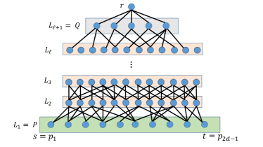
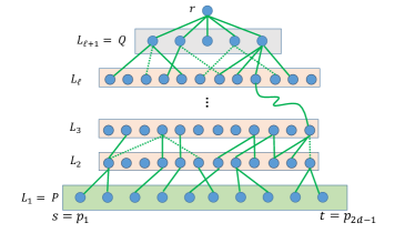
Figure 1: Left: An illustration of the auxiliary graph $G_{P,Q,\ell}$ and the BFS tree $T_{P,Q,\ell}$ shown in green. Each node in $P$ is connected by an $(\ell+1)$-length path to the root in $T_{P,Q,\ell}$. Right: The sampled graph $T^{*}$ is obtained by sampling each of the BFS edges between layers $L_{i}$ and $L_{i+1}$ independently with probability of $\mathbf{p}=n^{-1/(D-1)}$, for every $i\in\{1,\ldots,\ell\}$. The sampled edges of $T^{*}$ are shown in dashed.

To avoid cumbersome notation, let $T^{*}=T^{*}_{P,Q,\ell}$. The key lemma in our context is the following. Let $s=p_{1}$ and $t=p_{2d-1}$.

Lemma 3.2.

W.h.p., either $\mbox{\rm dist}_{T^{*}}(s,t)=O(k_{D})$, or else it must hold (w.h.p.) that $\mbox{\rm dist}_{T^{*}}(s,L_{j})=O(k_{D})$ for every $j\in\{2,\ldots,\min\{\ell+1,D/2+1\}\}$. The high probability guarantee

To prove Lemma 3.2 we introduce the notion of $(i,k)$ walks. Throughout, the randomized arguments are applied over the sampling of the edges of $T_{P,Q,\ell}$ into $T^{*}$.

Probabilistic analysis of $(i,k)$ walks.

An $(i,k)$ walk in the graph $T^{*}$ is a walk that starts at a node $p_{i}$ (the $i^{th}$ node of the path $P$, in layer $1$) and ends at some node in the set $V^{+}_{i}(P)\cup L_{k}$ where $V^{+}_{i}(P)=[p_{i},\ldots,p_{2d-1}]$. To describe the structure of a legal $(i,k)$ walk, it is convenient to view the nodes in layer $L_{1}$ of $T^{*}$ ordered from left to right, namely, $L_{1}=V(P)=(p_{1},\ldots,p_{2d-1})$.

Definition 3.1 ($(i,k)$ unit).

An $(i,k)$ unit is a walk that starts at node $p_{i}$ and ends at node $p_{j}$ for $j\geq i$ defined as follows. Let $u_{i,k}$ be the up-most ancestor of $p_{i}$ in $T^{*}\cap\bigcup_{\ell=2}^{k}L_{\ell}$. That is, the ancestor of $p_{i}$ in the maximum layer $\ell\leq k$. Letting $p_{j}$ be the right-most $P$-node (i.e., node of largest $j$ index on $P$) in the subtree of $T^{*}(u_{i,k})$, then the $(i,k)$ unit is defined by the $T^{*}$-walk:

$$P^{\prime}=\pi_{T^{*}}(p_{i},u_{i,k})\circ\pi_{T^{*}}(u_{i,k},p_{j})~{}.$$

Note that $(i,k)$ unit is indeed a walk (and not a simple path), in the case where the least-common-ancestor of $p_{i}$ and $p_{j}$ in $T^{*}$ is strictly below (i.e., in a smaller level then) $u_{i,k}$. A maximal $(i,k)$ walk is a walk $P^{\prime\prime}$ defined by applying $2d-i$ steps defined as follows. Initially, let $P_{1}$ be an $(i,k)$ unit, and let $p_{i_{1}}$ be the second endpoint of $P_{1}$, thus $i_{1}\geq i$. At any step $j\in\{1,\ldots,2d-i\}$, let $P_{j}$ be a walk ending at some node $p_{i_{j}}$. If $p_{i_{j}}=t$, then let $P_{j+1}=P_{j}$. Otherwise, let $P^{\prime}_{j}$ be an $(i_{j}+1,k)$-unit, and define $P_{j+1}=P_{j}\circ(p_{i_{j}},p_{i_{j}+1})\circ P^{\prime}_{j}$. The maximal $(i,k)$ walk is given by $P^{\prime\prime}=P_{2d-i}$. An $(i,k)$-walk is any sub-walk of a maximal $(i,k)$ walk. See Fig. 2 for an illustration.

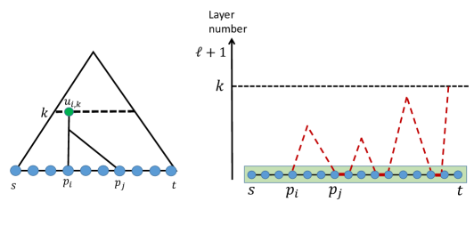
Figure 2: Left: The forest $T^{*}$ and an $(i,k)$ unit $P^{\prime}=\pi_{T^{*}}(p_{i},u_{i,k})\circ\pi_{T*}(u_{i,k},p_{j})$, where $j\geq i$. Since the least-common-ancestor of $p_{i},p_{j}$ in $T^{*}$ is below $u_{i,k}$, $P^{\prime}$ is indeed a walk (and not a simple path). Note that $P^{\prime}$ contains a unique $k$-level node, namely, $u_{i,k}$. Right: an $(i,k)$ walk made by concatenating $(j,k)$ walks, for increasing $j$ values, interleaved with edges from $P$.

Let $P^{\prime}=[p_{i}=u_{1},\ldots,u_{b}]$ be an $(i,k)$ walk, and consider the subset of $P$-nodes in $P^{\prime}$ ordered according to their appearance in $P^{\prime}$. We first observe that the sequence of nodes in $P^{\prime}$ is monotone in the sense of being sorted from left to right. Also observe that $P^{\prime}$ can be written as a concatenation of walks $P^{\prime\prime}=[u,v]$ where $u\in P$ and $v\in P\cup L_{k}$.

Observation 3.1.

Let $w_{1},\ldots,w_{a}$ be the multi-set of level $k$ nodes (i.e., in $L_{k}$) of an $(i,k)$ walk $P^{\prime}$ sorted according to their appearance on $P^{\prime}$ (in increasing distance from $p_{i}$). Then, $w_{j}\neq w_{j^{\prime}}$ for every $j\neq j^{\prime}\in\{1,\ldots,a\}$.

Proof:   Let $P_{1},\ldots,P_{a}$ be the $(i_{j},k)$ units composing $P^{\prime}$ such that $w_{j}\in P_{j}$ for every $j\in\{1,\ldots,a\}$. Note that each $P_{j}$ contains a unique level $k$ node. It then holds that $i<i_{1}<i_{2}\ldots<i_{a}$. Assume towards contradiction that $w_{j}=w_{j^{\prime}}$ where $j<j^{\prime}$. By the definition of $P_{j^{\prime}}$, we have that $p_{i_{j^{\prime}}}$ is in the sub-tree of $w_{j}=w_{j^{\prime}}$, in contradiction to the definition of $P_{j}$ which ends in a node $p_{i_{g}}$ for $i_{g}<i_{j^{\prime}}$. The claim follows.     

The key lemma in our context shows that w.h.p. the graph $T^{*}$ contains short $(i,k)$ walks for every $i$ and $k$.

Lemma 3.3.

For every $i\in\{1,\ldots,2d-1\}$ and $k\in\{2,\ldots,\ell+1\}$, $T^{*}$ contains an $(i,k)$ walk between $p_{i}$ to a node in $\{t\}\cup L_{k}$ of length at most $(c\cdot k_{D}/N)^{-k+2}$ for a sufficiently large constant $c\geq 8$, w.h.p. Moreover, this high probability guarantee uses at most $k$ out of $D$ (independent) repetitions of Step (2).

Proof:   The proof is shown by induction on $k$. The base case of $k=2$ follows for every $i\in\{1,\ldots,2d-1\}$, as all edges of $E(L_{1},L_{2})\cap T_{P,Q,\ell}$ are kept in $T^{*}$ with probability of $1$. Let $R_{i,k}$ be an indicator random variable for the event that there exists an $(i,k)$ walk of length at most $\ell_{k}=(c\cdot k_{D}/N)^{-k+2}$ ending at some node in $L_{k}\cup\{t\}$.

Assume that w.h.p. $R_{i,k}=1$ for every $i\in\{1,\ldots,2d-1\}$. We next show that also $R_{i,k+1}$ holds w.h.p. for every $i$. Let $R_{k}$ be the indicator random variable that $R_{i,k}=1$ for every $i\in\{1,\ldots,|P|\}$. Thus, by induction hypothesis, $R_{k}=1$ w.h.p. as well. Next, observe that

$$Pr[R_{i,k+1}]\geq Pr[R_{i,k+1}~{}\mid~{}R_{k}]\cdot Pr[R_{k}]~{}.$$

As $Pr[R_{k}]\geq 1-1/n^{c^{\prime\prime}}$ for some constant $c^{\prime\prime}\geq 2$, it is sufficient to bound the probability $Pr[R_{i,k+1}~{}\mid~{}R_{k}]$. To do that, we fix an $i\in\{1,\ldots,2d-1\}$, and bound the probability of having a particular $(i,k+1)$ walk. We define a walk $P^{\prime}$ that starts at $p_{i}$ and ends at a $P$-node. The walk $P^{\prime}$ is defined in $\ell=(c/2)\cdot N/k_{D}$ steps. Let $P_{1}$ be an $(i,k)$ unit. In step $j\in\{1,\ldots,\ell-1\}$, we are given a path $P_{1}\circ\ldots\circ P_{j}$ that ends in $p_{d_{j}}$. If $p_{d_{j}}\neq t$, let $P_{j+1}=(p_{d_{j}},p_{d_{j}+1})\circ P^{\prime}_{j+1}$, where $P^{\prime}_{j+1}$ is an $(d_{j}+1,k)$ unit. Otherwise (if $p_{d_{j}}=t$), $P_{j+1}=\emptyset$.

Let $P^{\prime}=P_{1}\circ P_{2}\circ\ldots\circ P_{\ell}$. If $P^{\prime}$ ends in $t$, we are done since $|P^{\prime}|\leq\ell(\ell_{k}+1)\leq\ell_{k+1}$. It remains to consider the case where none of the $P_{j}$ paths ends in $t$. For every path $P_{j}$ for $j\in\{1,\ldots,\ell\}$, let $w_{j}$ be the unique level-$k$ node in $L_{k}\cap V(P_{j})$. Since $P^{\prime}$ is an $(i,k)$ walk, by Obs. 3.1, $w_{j}\neq w_{j^{\prime}}$ for every $j\neq j^{\prime}\in\{1,\ldots,\ell\}$. We now show how to use $P^{\prime}$ to obtain an $(i,k+1)$ walk of length at most $\ell_{k+1}$. To see this, let $e_{j}=(w_{j},par(w_{j}))$ be the edge connecting $w_{j}$ to its parent in the tree $T_{P,Q,\ell}$. By the observation, $e_{j}\neq e_{j^{\prime}}$ for every $j\neq j^{\prime}\in\{1,\ldots,\ell\}$. As each edge $e_{j}$ is sampled independently into with probability $\mathbf{p}$ into $T^{*}$, the probability that at least one of these edges, say $e_{j}$, is in $T^{*}$ is at least

$$1-(1-\mathbf{p})^{\ell}=1-(1-\log n\cdot k_{D}/N)^{(c/2)\cdot N/k_{D}}\geq 1-1/n^{c/3}~{}.$$

This yields the $(i,k+1)$ walk $P^{\prime\prime}=P^{\prime}[p_{i},w_{j}]\circ(w_{j},par(w_{j}))$ of length at most $\ell\cdot(\ell_{k}+2)\leq\ell_{k+1}$ as desired. Note that the bound on $(i,k)$ walks only exploits the randomness in the sampled sets $E_{1},\ldots,E_{k}$, i.e., the first $k$ sampling repetitions of Step (2).     

Lemma 3.2 then follows by applying Lemma 3.3 with $i=1$ (as $p_{1}=s$) and $k\leq D/2+1$. Note that for $k=D/2+1$, the length of the $(1,k)$ walk is bounded by $(c\cdot k_{D}/N)^{-D/2+1}=O(k_{D})$ as desired. Next, we show the equivalence between an $(i,k)$ walk in $T^{*}$ to a corresponding path in the subgraph $H$ (for which we provide the diameter bound).

Observation 3.2.

Let $P^{\prime}$ be an $(i,k)$ walk of length $\ell^{\prime}$ in $T^{*}$ with endpoints $p_{i}$ and $u\in V(P)\cup L_{k}$. Then, there exists a path in $H$ between $p_{i}$ and the $G$-copy of $u$ of length at most $\ell^{\prime}$.

By Lemma 3.2 and Obs. 3.2, we have:

Corollary 3.4.

Let $P,Q$ be such that $\mbox{\rm dist}_{G}(P,Q)\leq\ell$. Then, w.h.p, either $\mbox{\rm dist}_{H}(s,t)=O(k_{D})$ or else, for every $k\in\{2,\ldots,\min\{\ell+1,D/2+1\}\}$, there exists a node $u\in V(G)$ such that $\mbox{\rm dist}_{G}(u,Q)\leq\ell-k+1$ and $\mbox{\rm dist}_{H}(s,u)=O(k_{D})$. Moreover, the probabilistic argument uses at most $k$ repetitions out of the $D$ repetitions of Step (2) of the centralized construction.

3.2 Proof of Theorem 3.1

Equipped with the tool of shortcut trees and $(i,k)$ walks, we are now ready to provide the dilation argument of the subgraph $H=G[S_{j}]\cup H_{j}$. Our goal is to show that $\mbox{\rm dist}_{H}(s,t)=\widetilde{O}(k_{D})$ for a fixed pair $s,t$ in $S_{j}$. Let $P^{\prime}=[s=v_{1},\ldots,v_{2d-1}=t]$ be the $s$-$t$ shortest path in $G[S_{j}]$. The next key lemma shows that at least half of the path $P^{\prime}$ can be shortcut in $H$ into a path length of $\widetilde{O}(k_{D})$. Since this argument can be applied to any sub-path of $P^{\prime}$, the final dilation bound is obtained by a recursive application of that lemma. We show:

Lemma 3.5.

W.h.p., one of the three events must hold w.h.p (i) $\mbox{\rm dist}_{H}(v_{d+1},v_{2d-1})=O(k_{D})$, (ii) $\mbox{\rm dist}_{H}(v_{1},v_{d})=O(k_{D})$, or (iii) $\mbox{\rm dist}_{H}(v_{1},v_{2d-1})=O(k_{D})$.

Proof:   The proof is based on having $d+1$ applications of the shortcut trees of Section 3.1. See Fig. 3 for an illustration. Let $H_{1},H_{2}$ be the edges added to the subgraph in the first (resp., last) $D/2$ applications of Step (2) of the algorithm. We will show that w.h.p. over the randomness of the edges sampled to $H_{1}$, each of the $d$ applications of the shortcut trees satisfies a certain desired property. Then, conditioned on these properties, we show that the last $(d+1)^{th}$ application satisfies another property w.h.p. over the randomness of the edges sampled to $H_{2}$. Since there is a dependency here, and each application uses at most $D/2$ sampling steps of Step (2), over all we need $D$ sampling steps. (For the first $d$ applications, we use the same $D/2$ sampling steps, as there is no conditioning between these applications).

Let $P_{1}=[s=v_{1},\ldots,v_{d}]$ be the first half of the path $P^{\prime}$, and let $P_{2}=[t=v_{2d-1},\ldots,v_{d+1}]$ be the second half of the path, written in a reverse manner from $v_{2d-1}$ to $v_{d+1}$. We start by making $d$ applications of the shortcut tree constructions where for each $i\in\{1,\ldots,d\}$, we define $Q_{i}=\{v_{i}\}$ and the auxiliary graph $G_{P_{2},Q_{i},D}$, the tree $T_{P_{2},Q_{i},D}$ and the final graph $T^{*}_{i}=T_{P_{2},Q_{i},D}[\mathbf{p}]\cup E(P_{2})$.

By Cor. 3.4, it holds that w.h.p. one of the following two events hold for any $i\in\{1,\ldots,d\}$ using at the most $D/2$ repetitions of the edge sampling in Step (2) of the algorithm.

• (E1) There exists a node $v_{i_{j}}\in V(H)$ such that $\mbox{\rm dist}_{H}(v_{i_{j}},v_{2d-1})=(cN/k_{D})^{(D-2)/2}=O(k_{D})$ and $v^{\ell^{\prime}}_{i_{j}}$ for $\ell^{\prime}=D/2+1$ is a node in layer $\ell^{\prime}$ in $T^{*}_{i}$.

• (E2) $\mbox{\rm dist}_{H}(v_{d+1},v_{2d-1})=O(k_{D})$.

If there exists an index $i\in\{1,\ldots,d\}$ for which event (E2) holds, we are done. Assume from now on that the event (E1) holds w.h.p. for every $i\in\{1,\ldots,d\}$. Let $q_{i}=v_{i_{j}}$ and define $Q=\{q_{1},\ldots,q_{d}\}$. Note that the nodes $q_{i}$ are not necessarily distinct. Since each $q_{i}$ appears in level $D/2+1$ of the tree $T_{P_{2},\{v_{i}\},D}$, it holds that $\mbox{\rm dist}_{G}(v_{i},q_{i})\leq D/2$. Therefore $\mbox{\rm dist}(V(P_{1}),Q)\leq D/2$. We now apply again the shortcut tree construction and define the graphs $G_{P_{1},Q,D/2}$, $T_{P_{1},Q,D/2}$ (as in Sec. 3.1). The sampled sub-tree $T_{P_{1},Q,D/2}[\mathbf{p}]$ is based on the sampled edge set $E_{D/2+1},\ldots,E_{D}$ (i.e., the edges sampled in the last $D/2$ applications of Step (2)). Formally, letting $L_{1}=V(P_{1})$, $L_{D/2+1}=Q$ and $L_{D/2+2}=\{r\}$, then $T_{P_{1},Q,D/2}[\mathbf{p}]$ consists of the following edges:

• $(E(L_{1},L_{2})\cup E(L_{D/2+1},L_{D/2+2}))\cap T_{P_{1},Q,D/2}$,

• self-edges: $\{(v_{i}^{k},v_{i}^{k+1})\in E(L_{k},L_{k+1})\cap E(T_{P_{1},Q,D/2})~{}\mid~{}v_{i}\in L_{k},k\in\{2,\ldots,D/2\}\}$,

• sampled non self-edges: $\{(v_{i}^{k},v_{j}^{k+1})\in E(L_{k},L_{k+1})\cap E(T_{P_{1},Q,D/2})~{}\mid~{}(v_{i},v_{j})\in E_{D/2+k-1},k\in\{2,\ldots,D/2\}\}$.

Let $T^{*}_{1}=T_{P_{1},Q,D/2}[\mathbf{p}]\cup E(P_{1})$. By Cor. 3.4 it holds that w.h.p. (over the second set of $D/2$ repetitions of the edge-sampling in Step (2)) that one of the following two events holds:

• (E3) $\exists q_{i^{*}}\in V(H)\cap Q$ such that $\mbox{\rm dist}_{H}(v_{1},q_{i^{*}})=(cN/k_{D})^{(D-2)/2}=O(k_{D})$.

• (E4) $\mbox{\rm dist}_{H}(v_{1},v_{d})=O(k_{D})$.

If event (E4) holds we are done. Thus, consider the case where (E3) holds. By event (E2), we have the w.h.p. $\mbox{\rm dist}_{H}(q_{i},v_{2d-1})=O(k_{D})$ for every $i\in\{1,\ldots,d\}$. By combining with (E3) we have that $\mbox{\rm dist}_{H}(v_{1},v_{2d-1})\leq\mbox{\rm dist}_{H}(v_{1},q_{i^{*}})+\mbox{\rm dist}_{H}(q_{i^{*}},v_{2d-1})=O(k_{D})$ as required. The lemma follows.     

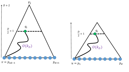
Figure 3: Illustration for the dilation argument of Theorem 3.1 for an $u$-$v$ shortest path $P=[s=v_{1},\ldots,t=v_{2d-1}]$. The argument applies $d+1$ applications of the shortcut trees scheme. Left: An illustration for the auxiliary graph $T^{*}_{i}=T_{P_{2},Q_{i},D}[\mathbf{p}]\cup E(P_{2})$. W.h.p., $T^{*}_{i}$ contains either (i) an $v_{2d-1}$-$v_{d}$ path of length $O(k_{D})$ or else (ii) an $v_{2d-1}$-$q_{i}$ path of length $O(k_{D})$ for some node $q_{i}$ in level $D/2+1$ of the tree $T_{P_{2},Q_{i},D}$. Right: The second part of the argument applies the shortcut construction for the auxiliary graph $T^{*}_{1}=T_{P_{1},Q,D}[\mathbf{p}]\cup E(P_{1})$ where $Q$ is the collection of $q_{i}$ nodes defined by the prior $d$ applications, for each $v_{i}\in P_{1}$. W.h.p., it then holds that $T^{*}_{1}$ contains either (i) an $v_{1}$-$v_{d}$ path of length $O(k_{D})$ or else (ii) an $v_{1}$-$q_{i}$ path of length $O(k_{D})$ for some node $q_{i}$. In the latter case, we obtain an $v_{1}$-$v_{2d-1}$ shortcut path of length $O(k_{D})$ that goes through $q_{i}$.

Proof:  [Proof of Theorem 3.1] Consider $s,t\in G[S_{j}]$ and let $P=[s=v_{1},\ldots,v_{2d-1}=t]$ be an $s$-$t$ shortest path in $G[S_{j}]$. By Lemma 3.5, it holds that it least half of the $s$-$t$ shortest path $P\subseteq G[S_{j}]$ can be shorten by a path of length $K=O(k_{D})$. In the same manner, we apply Lemma 3.5 on any subpath $P^{\prime}\subseteq P$. Since there are at most $|P|^{2}$ such paths, by the union bound, the guarantee of Lemma 3.5 holds for any such sub-path $P^{\prime}\subseteq P$.

Coming back to our path $P$, by Lemma 3.5 the shortcut argument can be applied recursively on the remaining path $P^{\prime}$ where $|P^{\prime}|\leq|P|/2$. Since in each recursive application w.h.p. there is a shortcut in one of the two bisections of the path, overall we obtain an $s$-$t$ path in $H$ of length $(k_{D}\log n)$ w.h.p.

To handle the case where the diameter is odd, the algorithm is modified as follows. We split each edge $e=(u,v)$ in $G$ into two edges by introducing a dummy intermediate node $x_{e}$ connected (only) to $u$ and $v$. The resulting modified graph $G^{\prime}$ has now an even diameter $D^{\prime}=2D$. Note that any path in $G^{\prime}$ corresponds to a path in $G$ in the following manner: The shortcut algorithm is applied on the graph $G^{\prime}$ where the only modification is that the sampling probability of each edge in $G^{\prime}$ is set to $\mathbf{p}^{\prime}=\sqrt{\mathbf{p}}$ (except for the edges chosen in Step $1$ of the algorithm, for each such edge we take the two-length corresponding path with probability $1$). Note that two edges $(u,x_{e})$ and $(x_{e},v)$ are sampled into the shortcut subgraph $H^{\prime}_{j}$ with probability of $(\mathbf{p}^{\prime})^{2}=\mathbf{p}$. The final output subgraph $H_{j}$ contains only edges $(u,v)$ such that both $(u,x_{e})$ and $(x_{e},v)$ are sampled into $H^{\prime}_{j}$. We then apply the argument similarly to the even diameter case. More specifically, we will be working on the graph $G^{\prime}$ all along. Then, in Lemma 3.5 the set $Q$ defined based on the first $d$ applications of the shortcut tree argument correspond to dummy nodes. Then, the $(d+1)^{th}$ application shows that either there is a short $G^{\prime}$ path of length $O(k_{D})$ between the endpoints $s,t$ of the path, or a shortcut of length $O(k_{D})$ between a path endpoint to a mid-point on the path. The reason that the length remains $O(k_{D})$ in this construction is that a path from level $1$ to level $D+1$ in the shortcut tree of $G^{\prime}$ contains $D-2$ edges where each edge was chosen with probability $\sqrt{\mathbf{p}}$ (we do not take into account the first two edges as they were chosen with probability $1$ into the shortcut subgraph), and thus the path length is $O(k_{D})$ by the application of Lemma 3.3 and Lemma 3.5. The rest of the argument is almost identical to the even case and thus omitted.     

4 Applications to Distributed Optimization

Fact 4.1 ([Gha17]).

Let $\mathcal{G}$ be a graph family such that for each graph $G\in\mathcal{G}$ and any partition of $G$ into vertex-disjoint connected graphs $G_{1},\ldots,G_{N}$, one can find an $(\mbox{\tt c},\mbox{\tt d})$ shortcuts such that $\mbox{\tt c}+\mbox{\tt d}\leq K$ and these shortcuts can be computed in $\widetilde{O}(K)$ rounds. Then:

• [Theorem 6.1.2]: there is a randomized distributed MST algorithm that computes an MST in $\widetilde{O}(K)$ rounds, with high probability, in any graph from the family $G$.

• [Theorem 7.6.1]: there is a randomized distributed algorithm that computes a $(1+\epsilon)$ approximation of the minimum cut in $\widetilde{O}(K)$ rounds, with high probability, in any graph from the family $G$.

Corollary 1.2 follows by combining Fact 4.1 with Theorem 1.1. An additional immediate corollary of improved shortcuts is for computing an approximate SSSP. Haeupler and Li [HL18] provided improved algorithms for several shortest-path problems whose bounds depend on the quality of shortcuts. By plugging the bounds of Theorem 1.1 into Corollaries 2,3 in [HL18] we get:

Corollary 4.2 (Improved Distributed SSSP Tree Algorithms).

There are randomized algorithms, that, given an $n$-vertex weighted graph with polynomial edge weights of unweighted diameter $D=O(1)$ perform the following tasks: (1) compute a spanning tree that approximates distances to a given source vertex to within factor $(\log n)^{O(1/\epsilon)})$, in $\widetilde{O}(n^{(D-2)/(2D-2)})\cdot n^{\epsilon})$ rounds for any constant $\epsilon$; and (2) compute a spanning tree that approximates distances to a given source vertex within factor $2^{O(\sqrt{\log n})}$, in $\widetilde{O}(n^{(D-2)/(2D-2)})\cdot 2^{O(\sqrt{\log n})})$ rounds.

Finally, Dory and Ghaffari [DG19] recently studied the distributed approximation of minimum weight two-edge connected subgraphs ($2$-EECS). By plugging Theorem 1.1 into Theorem 1.2 of [DG19], we get:

Corollary 4.3 (Improved Approximation of $2$-EECS).

There is an algorithm, that, given an $n$-vertex weighted graph of (unweighted) diameter $D=O(1)$, computes an $O(\log n)$-approximation of the weighted 2-ECSS in $\widetilde{O}(n^{(D-2)/(2D-2)})$ rounds, with high probability.

Acknowledgments.

We are very grateful to the PODC 2021 reviewers for many insightful comments, and specifically for the reviewer suggesting the improvement of Lemma 3.3.

References

- [AJB99] Réka Albert, Hawoong Jeong, and Albert-László Barabási. Diameter of the world-wide web. nature, 401(6749):130–131, 1999.
- [CPT20] Julia Chuzhoy, Merav Parter, and Zihan Tan. On packing low-diameter spanning trees. In 47th International Colloquium on Automata, Languages, and Programming, ICALP 2020, July 8-11, 2020, Saarbrücken, Germany (Virtual Conference), pages 33:1–33:18, 2020.
- [DG19] Michal Dory and Mohsen Ghaffari. Improved distributed approximations for minimum-weight two-edge-connected spanning subgraph. In Proceedings of the 2019 ACM Symposium on Principles of Distributed Computing, pages 521–530, 2019.
- [Elk04] Michael Elkin. Unconditional lower bounds on the time-approximation tradeoffs for the distributed minimum spanning tree problem. In Proceedings of the 36th Annual ACM Symposium on Theory of Computing, Chicago, IL, USA, June 13-16, 2004, pages 331–340, 2004.
- [GH16] Mohsen Ghaffari and Bernhard Haeupler. Distributed algorithms for planar networks II: low-congestion shortcuts, mst, and min-cut. In Robert Krauthgamer, editor, Proceedings of the Twenty-Seventh Annual ACM-SIAM Symposium on Discrete Algorithms, SODA 2016, Arlington, VA, USA, January 10-12, 2016, pages 202–219. SIAM, 2016.
- [GH20] Mohsen Ghaffari and Bernhard Haeupler. Low-congestion shortcuts for graphs excluding dense minors. CoRR, abs/2008.03091, 2020.
- [Gha15] Mohsen Ghaffari. Near-optimal scheduling of distributed algorithms. In Proceedings of the 2015 ACM Symposium on Principles of Distributed Computing, pages 3–12. ACM, 2015.
- [Gha17] Mohsen Ghaffari. Improved Distributed Algorithms for Fundamental Graph Problems. PhD thesis, MIT, USA, 2017.
- [GKS17] Mohsen Ghaffari, Fabian Kuhn, and Hsin-Hao Su. Distributed MST and routing in almost mixing time. In Proceedings of the ACM Symposium on Principles of Distributed Computing, PODC 2017, Washington, DC, USA, July 25-27, 2017, pages 131–140, 2017.
- [GP16] Mohsen Ghaffari and Merav Parter. MST in log-star rounds of congested clique. In Proceedings of the 2016 ACM Symposium on Principles of Distributed Computing, PODC 2016, Chicago, IL, USA, July 25-28, 2016, pages 19–28, 2016.
- [GP17] Mohsen Ghaffari and Merav Parter. Near-optimal distributed DFS in planar graphs. In 31st International Symposium on Distributed Computing, DISC 2017, October 16-20, 2017, Vienna, Austria, pages 21:1–21:16, 2017.
- [HHW18] Bernhard Haeupler, D. Ellis Hershkowitz, and David Wajc. Round- and message-optimal distributed graph algorithms. In Proceedings of the 2018 ACM Symposium on Principles of Distributed Computing, PODC 2018, Egham, United Kingdom, July 23-27, 2018, pages 119–128, 2018.
- [HIZ16] Bernhard Haeupler, Taisuke Izumi, and Goran Zuzic. Low-congestion shortcuts without embedding. In Proceedings of the 2016 ACM Symposium on Principles of Distributed Computing, pages 451–460. ACM, 2016.
- [HL18] Bernhard Haeupler and Jason Li. Faster distributed shortest path approximations via shortcuts. In 32nd International Symposium on Distributed Computing, DISC 2018, New Orleans, LA, USA, October 15-19, 2018, pages 33:1–33:14, 2018.
- [HLZ18] Bernhard Haeupler, Jason Li, and Goran Zuzic. Minor excluded network families admit fast distributed algorithms. In Proceedings of the 2018 ACM Symposium on Principles of Distributed Computing, PODC 2018, Egham, United Kingdom, July 23-27, 2018, pages 465–474, 2018.
- [HPP+15] James W. Hegeman, Gopal Pandurangan, Sriram V. Pemmaraju, Vivek B. Sardeshmukh, and Michele Scquizzato. Toward optimal bounds in the congested clique: Graph connectivity and MST. In Proceedings of the 2015 ACM Symposium on Principles of Distributed Computing, PODC 2015, Donostia-San Sebastián, Spain, July 21 - 23, 2015, pages 91–100, 2015.
- [JN18] Tomasz Jurdzinski and Krzysztof Nowicki. MST in O(1) rounds of congested clique. In Proceedings of the Twenty-Ninth Annual ACM-SIAM Symposium on Discrete Algorithms, SODA 2018, New Orleans, LA, USA, January 7-10, 2018, pages 2620–2632, 2018.
- [KKOI19] Naoki Kitamura, Hirotaka Kitagawa, Yota Otachi, and Taisuke Izumi. Low-congestion shortcut and graph parameters. In Jukka Suomela, editor, 33rd International Symposium on Distributed Computing, DISC 2019, October 14-18, 2019, Budapest, Hungary, volume 146 of LIPIcs, pages 25:1–25:17. Schloss Dagstuhl - Leibniz-Zentrum für Informatik, 2019.
- [LMR99] Tom Leighton, Bruce Maggs, and Andrea W Richa. Fast algorithms for finding O(congestion+ dilation) packet routing schedules. Combinatorica, 19(3):375–401, 1999.
- [LP19] Jason Li and Merav Parter. Planar diameter via metric compression. In Proceedings of the 51st Annual ACM SIGACT Symposium on Theory of Computing, STOC 2019, Phoenix, AZ, USA, June 23-26, 2019, pages 152–163, 2019.
- [LPP01] Zvi Lotker, Boaz Patt-Shamir, and David Peleg. Distributed MST for constant diameter graphs. In Proceedings of the Twentieth Annual ACM Symposium on Principles of Distributed Computing, PODC 2001, Newport, Rhode Island, USA, August 26-29, 2001, pages 63–71, 2001.
- [LPP06] Zvi Lotker, Boaz Patt-Shamir, and David Peleg. Distributed MST for constant diameter graphs. Distributed Comput., 18(6):453–460, 2006.
- [LPPSP03] Zvi Lotker, Elan Pavlov, Boaz Patt-Shamir, and David Peleg. MST construction in O() communication rounds. In the Proceedings of the Symposium on Parallel Algorithms and Architectures, pages 94–100. ACM, 2003.
- [Now19] Krzysztof Nowicki. A deterministic algorithm for the MST problem in constant rounds of congested clique. CoRR, abs/1912.04239, 2019.
- [Pel00] David Peleg. Distributed Computing: A Locality-sensitive Approach. Society for Industrial and Applied Mathematics, Philadelphia, PA, USA, 2000.
- [SHK+11] Atish Das Sarma, Stephan Holzer, Liah Kor, Amos Korman, Danupon Nanongkai, Gopal Pandurangan, David Peleg, and Roger Wattenhofer. Distributed verification and hardness of distributed approximation. In Proceedings of the 43rd ACM Symposium on Theory of Computing, STOC 2011, San Jose, CA, USA, 6-8 June 2011, pages 363–372, 2011.
- [SHK+12] Atish Das Sarma, Stephan Holzer, Liah Kor, Amos Korman, Danupon Nanongkai, Gopal Pandurangan, David Peleg, and Roger Wattenhofer. Distributed verification and hardness of distributed approximation. SIAM Journal on Computing, 41(5):1235–1265, 2012.