Observation of Universality in Decaying Turbulence

Abstract

A hallmark of fluid turbulence theory is the universal power law scaling of the velocity difference statistics between two points in space in the inertial range between the large energy injection scale and the small energy dissipation scale. Even at the highest Reynolds numbers available, laboratory and natural flows such universal power laws have not been convincingly demonstrated. Here we show for the decaying active grid turbulence of the Max Planck Variable Density Turbulence Tunnel [1, 2] that the velocity difference statistics at high Reynolds numbers do not exhibit a power law, but have a universal functional form independent of the Reynolds number. We separate this functional form from the power law exponent and discuss potential consequences for turbulence modelling.

Turbulence in a three-dimensional incompressible fluid can be described by a flow of kinetic energy from large energy injection length scales $L$ to small viscous scales $\eta$, where internal friction dissipates this kinetic energy into heat. For intermediate scales, i.e., in the inertial range, the statistics of turbulent velocity fluctuations are described by the moments of two-point velocity increments [3]. The $n$-th order moments of velocity increments are called structure functions, $S_{n}(r)=\langle(u(x+r)-u(x))^{n}\rangle$. The separation between large and small scales, or the size of the inertial range, goes hand in hand with the magnitude of the main parameter capturing the intensity of a turbulent flow, which is the Taylor-scale Reynolds number $R_{\lambda}=u_{RMS}\lambda/\nu$. $u_{RMS}$ is the root-mean-squared velocity fluctuation, $\nu$ is the kinematic viscosity of the fluid, and $\lambda$ is the length scale defined in Taylor [4], where $L\gg\lambda\gg\eta$.

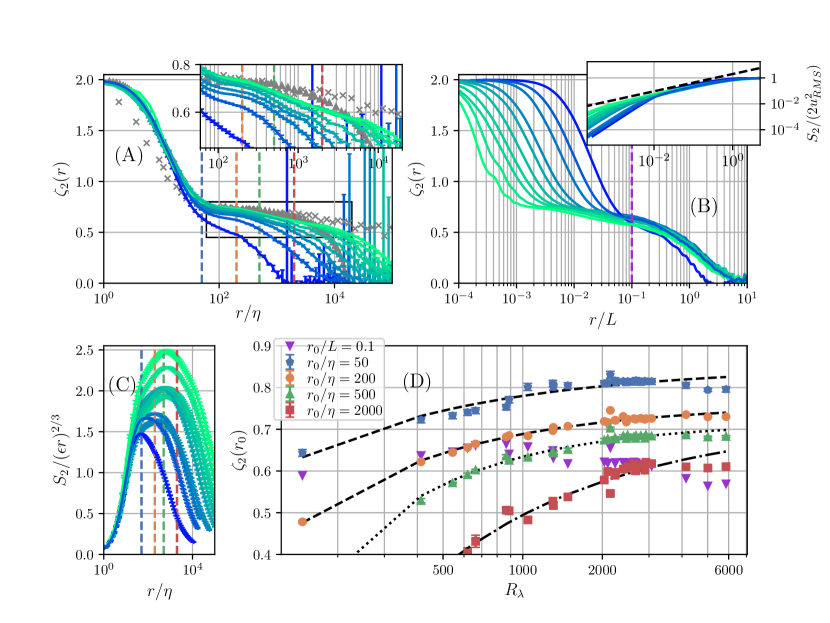
Figure 1: (A): $\zeta_{2}(r)$ for $R_{\lambda}$ = 150, 410, 660, 890, 1480, 2030, 2680, 3070, 4140 and 5860. The curves collapse approximately onto a universal form for $R_{\lambda}>2000$ at scales extending up to 1000$\eta$ ($\approx 0.1L$) as seen in the inset. This form extends from the smallest scales up to $0.1L$ and is different from a constant, which indicates that power law scaling is masked in these data. In contrast, the curves at $R_{\lambda}<2000$ change shape significantly with $R_{\lambda}$. Grey triangles: direct numerical simulations at $R_{\lambda}=2250$ [5]. Grey crosses: atmospheric measurements [6]. Inset: Zoom on the inertial range of the same curves. Dashed lines: $r_{0}/\eta$ for the curves in (D). (B): Same as (A), but normalised by $L$. At the largest scales the curves follow a similar shape from the largest scales down to $0.2L$. Dashed line: $r_{0}/L$ for the curve in (D). Inset: $S_{2}$ normalised by its large scale expectation value of $u_{RMS}^{2}$. Dashed line: $\sim r^{2/3}$. The transition from the approximate inertial range to the large-scale dominated range is at $r/L>0.1$. (C): Structure functions $S_{2}$ compensated by the scale-invariant prediction, $(\varepsilon r)^{2/3}$. (D): $\zeta_{2}(r)$ evaluated at fixed $r_{0}/\eta$ given by the dashed lines in (A), and fixed $r_{0}/\eta$ given by the curve in (B). Error bars smaller than symbols in most cases. To the extent that the curves approach constants, these constants depend on $r_{0}$. Therefore, no single scaling exponent $\bar{\zeta_{2}}$ can be isolated. Dashed lines are fits of $\alpha_{1}-\alpha_{2}R_{\lambda}^{\beta}$ to the data. Note that the inertial range as we define it here extents from $\approx 100\eta$ to $\approx 0.1L$. Where shown, vertical errorbars indicate a 95%-CI from 30- or 100-second sections of the hours-long datasets and a 4%-error on the mean velocity in $r=U\Delta t$.

A fundamental question is to what extent turbulent self-organisation leads to universal statistics such as $S_{n}(r)$. In this context universality is understood as the collapse of statistics for flows of very different origin independent of Reynolds number upon proper normalisation. For example, in the inertial range the statistics of velocity increments should be the same for jets, wind tunnels, mixing flows, the atmospheric boundary layer or any other in-compressible flows at sufficiently large Reynolds number. This conjecture is closely related to Kolmogorov’s seminal 1941 work [3] where he posited for statistically isotropic, homogeneous turbulence that the flow-specific energy injection mechanisms impact the statistics only at large scales $\sim L$, but universal self-organisation prevails at scales $r\ll L$ down to the dissipation scale $\eta$. In this inertial range, the mean power per unit mass, $\varepsilon$, describes the energy transfer from energy injection scales to dissipative scales. Dimensional analysis then yields universal scaling laws for the inertial range structure functions

$$S_{n}(r)= \;C_{n}(\varepsilon r)^{\zeta_{n}}$$ (1)

$$\zeta_{n,K41}= \;n/3,$$ (2)

where $C_{n}$ are universal constants in Kolmogorov [3].

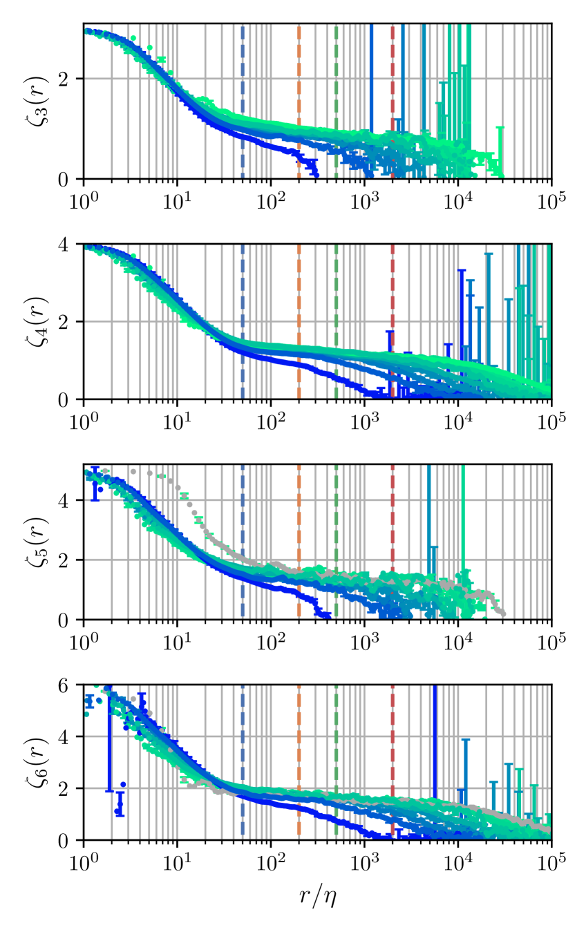
Figure 2: Same as Fig. 1 (A) but for orders $3<n\leq 6$, showing that the general trends observed at the second order are preserved at higher orders. $\zeta_{5}$ was smoothed using cubic splines, and those data do not converge as well at the highest $R_{\lambda}=5890$ in gray are likely influenced by a non-constant frequency response at small scales.

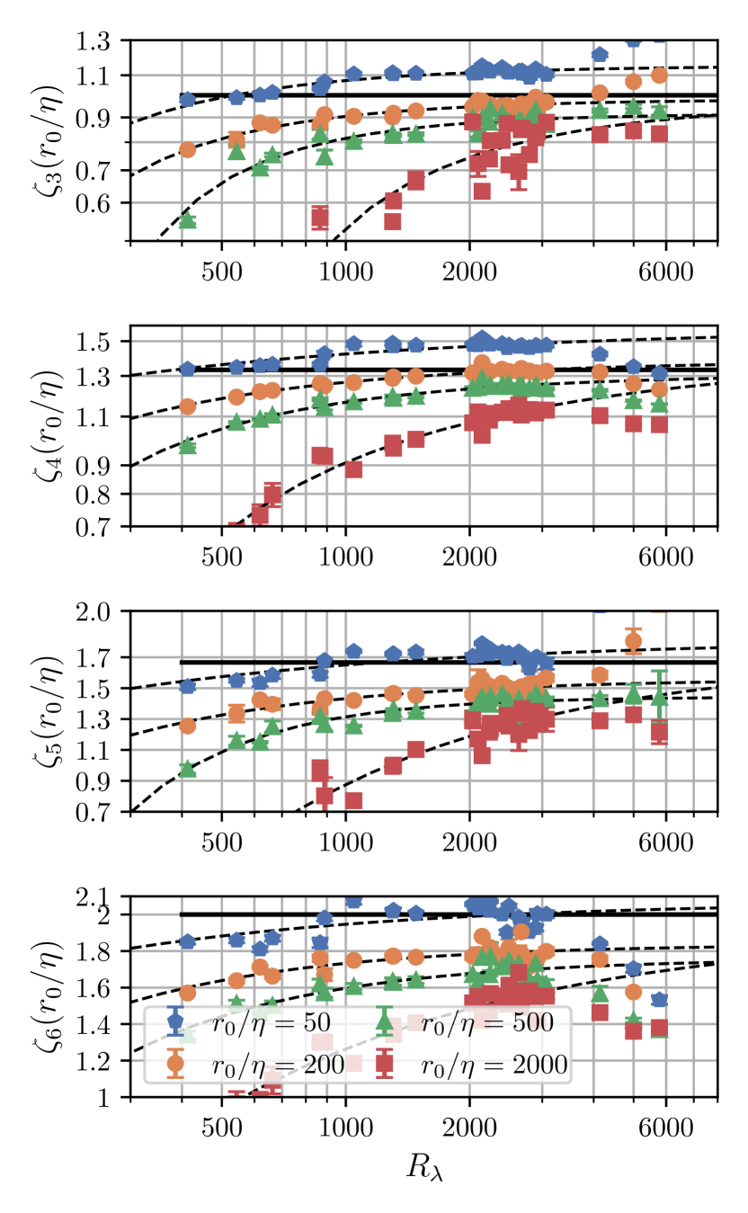
Figure 3: Same as Fig. 1 (D) but for $3<n\leq 6$, showing as in Fig. 2 that the trends observed at the second order are visible also at higher orders. The solid black lines show the result of Kolmogorov’s [3] dimensional analysis $\zeta_{n}=n/3$, which lies above the data for values of $r_{0}$ in the inertial range. Dashed lines are fits of $\alpha_{1}-\alpha_{2}R_{\lambda}^{\beta}$ to the data excluding the largest three $R_{\lambda}$.

The K41 scaling laws are still widely used approximations [7], even though we know that the intermittent spatial distribution of dissipation demands corrections [8, 9, 10]. While much effort has been invested in modelling intermittency corrections to the scaling exponents $\zeta_{n}$ [10, 11, 12, 13, 14, 15, 16, 17], the approach towards universal, $R_{\lambda}$-independent scaling laws at $R_{\lambda}\rightarrow\infty$ is rarely questioned. An exception is the work by Barenblatt and Goldenfeld [18], where a continued but potentially universal $R_{\lambda}$-dependence is assumed.

The scaling laws (1) have been derived under the idealised assumptions of a statistically stationary, homogeneous and isotropic flow in the limit of $\nu\rightarrow 0$. Direct numerical simulations (DNS) permit the study of non-decaying isotropic turbulence as the turbulence is forced continuously in the bulk. In both DNS and experiments, building controlled high Reynolds number turbulent remains a practical challenge. Adequately large Reynolds numbers were available up to recently only in natural atmospheric flows, which are inhomogeneous and non-stationary, or turbulence in (super)fluid helium [19, 20, 21, 22], where non-intrusive measurements are extremely challenging due to the small viscous length scales [23, 24, 25, 26, 27].

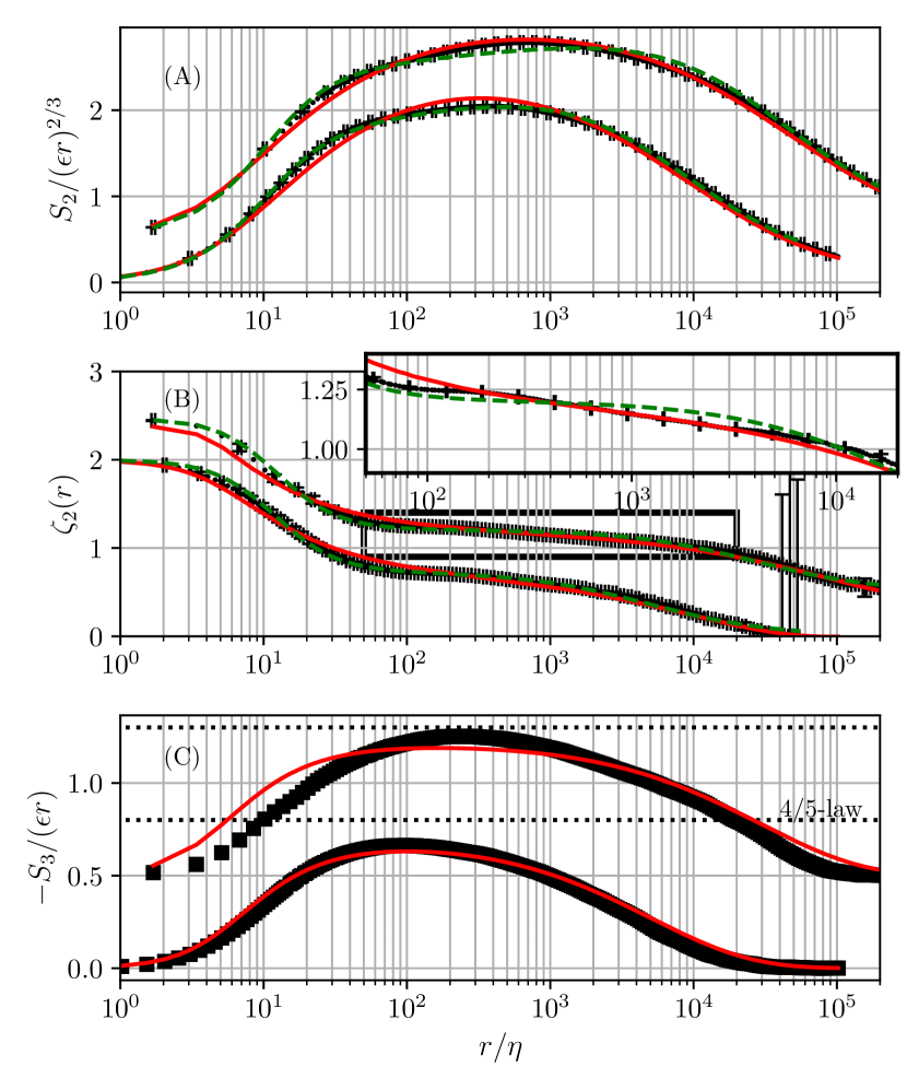
Figure 4: Comparisons of models (red, green) with experimental data (black) for two Reynolds numbers, $R_{\lambda}=1300$ (lower curves) and $R_{\lambda}=4140$ (upper curves, offset by 0.5 for clarity). Batchelor’s formula is shown as green dashed lines, and the model in Yang et al. [28] as red solid lines. (A) Fits of models to $S_{2}$ compensated by Kolmogorov’s prediction eq. (2). At large $R_{\lambda}$, the Batchelor formula assumes a more pronounced inertial range plateau than the data. (B) For power laws, the region of interest is the inertial range ($100<r/\eta<10000$ in the high-$R_{\lambda}$ case) as highlighted by the inset, and where the red curves follow the data more closely. For $r/\eta<100$ the Batchelor interpolation is superior, and the Yang et al. [28] model performs poorly as expected. At scales larger than those in the inertial range, both fits have a similar quality. (C) Fits of models to $-S_{3}$ compensated by Kolmogrov’s prediction eq. (2). The high-$R_{\lambda}$ asymptote (4/5) in the inertial range is indicated by horizontal dotted lines.

A large body of experimental and numerical data is available at lower $R_{\lambda}$. At these $R_{\lambda}$ and at low orders $n$, $S_{n}\sim r^{n/3}$ only approximates the existing data [e.g. 29, 30, 31]. This is because viscosity influences relatively large scales compared with the dissipation scale through the so called bottleneck [32, 33] shadowing the inertial range scaling in both experiments and numerical simulations [34, 35, 36, 37, 38].

In all experimental flows known to us the turbulence is generated locally in space and is decaying away from the source of turbulence. This is true for wind tunnels, wakes, jets, counter-rotating disks, vibrating grids, etc. These effects are known to adversely affect the buildup of power law scaling in the inertial range [39, 40, 31]. The effects of decay and anisotropic energy injection are typically stronger than those of the scale-local forcing in numerical simulations [34, 39, 41].

The effect of viscosity and the time-dependence of the flow on the velocity increment statistics can be assessed by statistically averaging Navier-Stokes equations. Assuming isotropy and homogeneity, but allowing for a term $P$ describing the time-dependence of a continuous forcing or decay, the Karman-Howarth-equation links structure functions of orders 2 and 3: [42, 43, 44, 45]

$$-S_{3}(r)=\frac{4}{5}\varepsilon r-6\nu\frac{\partial S_{2}}{\partial r}-P.$$ (3)

$P$ depends strongly on external conditions. The form of the statistics is typically written as

$$S_{n}=C_{n}~{}(\varepsilon r)^{n/3}\left(\frac{r}{L}\right)^{\mu_{n}}F_{n}(R_{\lambda},r/\eta).$$ (4)

Using closure models for the statistical evolution equations (3) [28, 41, 46], empirical parameterisations for $F_{n}$ [47, 48, 49, 50, 51], or physically motivated derivations of the large-scale terms [43, 46, 37, 28], functional forms for $F_{n}$ can be found to describe data. Extensive theoretical [39, 44, 43] and experimental [31, 52, 53, 45] efforts have been invested into the description of decay phenomena in this context. The results indicate that a dependence on $R_{\lambda}$ may not vanish before $\mathcal{O}(R_{\lambda})=10^{4}$ in decaying turbulence behind a passive grid.

In this article we show how velocity increment statistics approach a inertial range that is independent of the Reynolds number above $R_{\lambda}\approx 2000$ up to the experimental limit of $R_{\lambda}\approx 6000$. From this we conclude that $F_{n}(R_{\lambda},r/\eta)$ is a non-trivial, $R_{\lambda}$-independent and universal function at high Reynolds numbers in decaying turbulent flows.

We conducted experiments in the Max Planck Variable Density Turbulence tunnel which has a volume of 88m³ and is pressurized with sulphur hexaflouride (SF₆) at pressures between 1 and 15 bar, where an approximately homogeneous central region exists within the tunnel [1]. The turbulence was generated by an active grid, which dynamically blocks parts of the tunnel cross-section at variable length- and time scales [2, 33]. We have compared our data to that from a traditional passive grid in the same facility and they agree very well. We recorded time series of the streamwise velocity component using subminiature hot wires (Nanoscale Thermal Anemometry Probes, NSTAPs) [54] and conventional hot wires. The wire lengths were $\lesssim 4\eta$.

In eq. (4) we observe that the prefactors $C_{n}$ as well as the $r$-dependent remainder may depend on $R_{\lambda}$. To separate the scaling of the $n$-th order structure function $S_{n}$ from the constants $C_{n}$ we consider first the local power-law exponents

$$\zeta_{n}(r)=\frac{d\log(S_{n})}{d\log(r)}=\frac{n}{3}+\mu_{n}+\frac{d\log(F)}{d\log(r)}$$ (5)

Fig. 1 exemplifies our results at the second order for selected $R_{\lambda}$. In panels (A) and (B) we show the local power-law exponent $\zeta_{2}(r)$ with the scale $r$ normalised by the viscous length scale $\eta$ and the energy injection scale $L$, respectively. A power law prevails when $\zeta_{n}(r)$ assumes a constant value $\zeta_{n}=n/3+\mu_{n}$, which is the scaling exponent. We find that for small $r\approx\eta$, $\zeta_{2}\sim 2$ ($S_{2}\sim r^{2}$), as expected from continuity. Around $r\approx 100\eta$, $\zeta_{2}(r)$ flattens as expected for the inertial range. The width of this approximate plateau increases with $R_{\lambda}$, with a tilt evident even at the largest $R_{\lambda}$. This shape appears not to change starting around $R_{\lambda}\approx 2000$ and above. The tilt is also observed in recent DNS at $R_{\lambda}=2250$ [5] and atmospheric measurements at much larger $R_{\lambda}\approx 17000$[6], but is slightly less pronounced compared to our data. Due to these properties we define the approximate plateau in $\zeta_{2}$ as the inertial range for the remainder of this article. At yet larger scales, $\zeta_{2}(r)$ approaches zero, its large-scale limiting value for even $n$. Panel (C) of Fig. 1 shows the corresponding structure functions $S_{2}(r)$ compensated by the Kolmogorov prediction eq. (2). No clear plateau can be observed even at the largest $R_{\lambda}$ indicating the absence of plain scaling. To better illustrate the $R_{\lambda}$-dependence of the local power law exponent $\zeta_{2}(r)$ we plot its value at specific scales $r_{0}$ within the inertial range as functions of $R_{\lambda}$ in Fig. 1 (D). Overall, $\zeta_{2}(r_{0}/\eta)$ reaches a constant for $R_{\lambda}>2000$ and any fixed $r_{0}$ in the inertial range. Therefore, the shape of $(r/L)^{\mu_{n}}F_{n}(r/\eta)$ in the inertial range becomes independent of $R_{\lambda}$ for $R_{\lambda}>2000$. However, the particular asymptotic values of $\zeta_{n}(r_{0}/\eta)$ found at each specific scale $r_{0}/\eta$ in the inertial range differ by up to 0.2 – far more than typical intermittency corrections.

The above observations apply also at higher orders, which are shown in Figs. 2 and 3. At the largest $R_{\lambda}$ and smallest scales observed, the data are likely influenced by insufficient instrument frequency responses. This is particularly important at higher orders.

So far, we have found that we cannot infer a single inertial range exponent, and thus cannot disentangle $\mu_{n}$ from $F$ given a single structure function. We therefore turn to a model of decaying turbulence in a finite domain to aid us in separating $F$ and $\mu_{n}$. We compare the results from this analysis to an established empirical method to extract $\mu_{n}$.

In freely decaying turbulence, the energy injection scale $L$ grows over time [55, 56]. In the VDTT, however, the growth of $L$ is limited by the dimensions of the wind tunnel’s cross section. Decaying turbulence in a confined domain was recently modeled by Yang, Pumir and Xu [28]. The authors derive the functional forms for the viscous and large-scale cutoffs of inertial range power laws from a closure theory and self-similar decay laws (see Methods for details). In the model the effective scaling exponent of the second order structure function ($n/3+\mu_{2F}$) is one parameter, while the other describes the decay and is related to the normalised rate of dissipation $C_{\varepsilon}=\varepsilon L/u^{3}$. The model can thus be used to separate the inertial-range scaling from large-scale effects in the present experiments. An alternative is the ad-hoc formula in Refs [47, 50], which provides smooth transitions between the different scaling regimes ($r^{n}$,$r^{\zeta_{n}}$,$r^{0}$), but no physical justification.

In Fig. 4 we show the two models in red ([28]) and green ([50]) with parameters fitted to the experimental data. The fits indicate that the model for decaying turbulence in a confined domain [28] is a better approximation at higher Reynolds numbers than the Batchelor interpolation formulation[47, 50], whereas the Batchelor formula describes the data better at lower $R_{\lambda}$. Both models asymptotically approach power laws in the inertial range at very large $R_{\lambda}$. At second order the model in Yang et al. [28] better predicts the sustained influence of turbulence decay down to relatively small scales and is close to the data in the inertial range. At third order, the model performs well only at the smaller $R_{\lambda}$ chosen. At large $R_{\lambda}$, the model is already close to its asymptotic state of $S_{3}/(\varepsilon r)=\mathrm{const.}$ by construction in the inertial range. This asymptotic state differs qualitatively from the behaviour we observe, which explains the differences between the model and our data.

We interpret the model in Yang et al. [28] as a physical model for $(r/\eta)^{\mu_{n}}F_{2}(R_{\lambda},r/\eta)$ and extract the intermittency correction $\mu_{n}$ from the data.

In Fig. 5 we compare the intermittency correction $\mu_{2F}$ from this model of decaying turbulence [28] to an established empirical method for extracting $\mu_{2}$ from the data alone. This latter Extended Self Similarity (ESS) method was introduced in Benzi et al. [57] and assumes that $F_{n}\approx F_{|3|}$, such that ratios of different order structure functions show an extended scaling range with reduced effects of the finite Reynolds number and reduced uncertainty in the inertial-range scaling exponent $\zeta_{2,ESS}$. Phenomenological models potentially connected to this empirical observation can be found in [16, 17]. We find good agreement between this method of extended self-similarity (ESS) and the model parameter $\zeta_{2F}=\mu_{2F}+2/3$.

We are finally in the position to measure the universal modulation $F(R_{\lambda},r/\eta)$ at large Reynolds numbers and small scales $r<0.1L$ (the statistics of large scales inevitably depend on the flow geometry). For this we consider the curve

$$F_{2}(R_{\lambda},r/\eta)=\frac{S_{2}}{C_{2}(\varepsilon r)^{2/3}(r/\eta)^{\mu_{2}}}.$$ (6)

We determine $C_{2}$ by normalising the maximum of the resulting curves to 1 and by fixing $\mu_{2}=0.693$ from the ESS estimate. Fig. 5 (B) shows that $F_{2}$ begins to collapse around $R_{\lambda}\approx 1500$, i.e. assumes a universal form at high $R_{\lambda}$. To show this more clearly, we take $F(R_{\lambda}=4141)$ as an approximation towards this asymptotic form and plot the relative differences towards this reference. In the inset of Fig. 5 (A) we observe that starting around $R_{\lambda}\approx 1500$ the curves are within $\pm 3\%$ of each other.

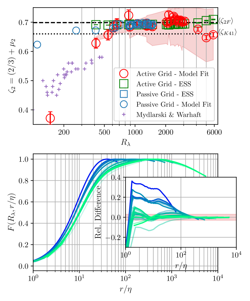
Figure 5: Upper Plot: The second-order scaling exponent $\zeta_{2}$ measured in different ways and in different laboratory experiments. Circles show $\zeta_{2}$ found by fitting eq.(10) to data from active and passive grid experiments. Squares show extended self-similarity (ESS) exponents, $S_{2}(|S_{3}|)$, for the same datasets. According to the model fits, $\zeta_{2}$ approaches a constant $\langle\zeta_{2F}\rangle=0.698\pm 0.011$ (dashed) larger than Kolmogorov’s prediction (dotted) [3]. We attribute the slight downward trend in the last two data points to probe effects and the anisotropic forcing that we used to reach these high $R_{\lambda}$. For comparison we include data from Mydlarski and Warhaft [30]. For $R_{\lambda}<300$, no ESS exponent could be measured due to an insufficient inertial range. The shaded region corresponds to the range of values that the local slope $\zeta_{2}(r)$ takes within $100\eta<r<0.1L$. Lower Plot: Approach of $F_{2}$ measured by eq. (6) towards an $R_{\lambda}$-universal shape. Starting around $R_{\lambda}\approx 1500$ the curves collapse for $r<0.1L$. Inset: The relative difference, $(F_{2}-F_{2}(R_{\lambda}=4141))/F_{2}(R_{\lambda}=4141)$ shows universality to within $\pm 3$% (indicated by the shaded area) for about three decades in $r$. The plots include measurements at a total of 29 different Reynolds numbers.

In this article we present experimental data that shows how the velocity increment statistics approach a fully-developed inertial range whose shape is independent of the Reynolds number. While this is in agreement with Kolmogorov’s hypothesis of universality, the scaling laws (and their intermittency corrections) anticipated for these conditions are not directly observed. That is, the inertial range is only approximately described by power laws and carries an apparently $R_{\lambda}$-independent modulation, $F_{2}(r/\eta)$ in eq. (6). Data from entirely different flow geometries, such as a jet [31], suggest that $F_{n}(r/\eta)$ is sensitive to the overall flow configuration for $n=3$, but less so for $n=2$. We observed little variation for different active grid schemes. A careful analysis of other high $R_{\lambda}$-data is of great interest in the light of our results. We also show that the widely used empirical ESS scheme to obtain the intermittency correction $\mu$ [57] gives an equivalent answer at second order to a physically motivated model of the entire structure function [28].

In decaying turbulence the inertial range grows more slowly than in continuously forced turbulence, and the time-dependent term in the statistical evolution equation does not vanish [34, 39, 45, 37, 28, 31]. Indeed, a model [28] for the decay of turbulence (confined as in our experiment) predicts an influence of the decay on its structure from large scales to deep into the inertial range and allows us to quantify the intermittency correction $\mu_{2}$. While the model we use is designed to approach an inertial range power law, our data suggest that above $R_{\lambda}\approx 2000$ the approach to a power law is halted. We show instead that above this Reynolds number the statistics are described by a universal and nontrivial shape from small scales up to $r\approx 0.1L$. This suggests that even models that consider large-scale effects, but prescribe an asymptotic approach to K41-like scaling laws fail to describe real flows at large $R_{\lambda}$.

When turbulence is not isotropic, scaling laws appear only when projecting onto appropriate symmetry groups [58, 59, 60]. The instrumentation in the present experiment allows only unidirectional velocity measurements, such that anisotropy can be inferred only indirectly. The measurements might therefore represent the approach to universality in anisotropic turbulence with little consequences for the idealised Kolmogorov framework. However, the measurement volume is relatively free of mean shear and the results are remarkably robust even when the turbulence is excited using an anisotropic active grid protocol or a classical and static grid.

We have shown that $F_{2}$ is a $R_{\lambda}$-independent and nontrivial function of the scale $r$ with indications from Figs. 2 and 3 that higher orders behave similarly. We point out that ESS means that $F_{n}$ is similar for all even orders. The processes that shape the asymptotic form of $F_{n}$ and that interfere with power-law scaling are evidently open questions. This already bears the potential for substantial advancements to applied turbulence models and the scaling seen in engineering wind tunnel studies. Future studies will need to investigate the degree to which $F_{n}$ changes from flow to flow at very large $R_{\lambda}$. While data from DNS [5] and atmospheric measurements [6] reproduced in Fig. 1 indicate some flow-dependent variability, a demonstration of the approach towards $R_{\lambda}$-independence is unique to the study at hand. A flow-independent function of the $n$-th order statistics, if it existed, would have far-reaching implications for turbulence models and closure schemes. Moreover, a theoretical understanding of the underlying universal mechanisms would be an important step towards an efficient simulation of turbulent flows.

To summarise, we claim that the route to universality in decaying turbulence is different from a simple removal of large-scale and viscous effects over some range of scales and the subsequent appearance of scaling laws. Past claims that this is simply an slow process [31, 53, 43] to occur at extremely large $R_{\lambda}$ only are at odds with our data, which shows universality, but no signs of the emergence of power laws. Our data is however plausible if scale-locality is not given or if large scales directly impact significantly smaller scales (and vice versa) as suggested in Refs. [61, 62, 63, 64, 32]

We end by commenting that deviations from power-law scaling in the inertial range have in the past been dismissed as finite Reynolds number effects that were to be circumvented. Viscous effects are important when the Reynolds number is low. Our results suggest however, that deviations from power-law scaling are an important feature of naturally occurring decaying turbulence, whatever its Reynolds number.

Appendix A Methods

A.1 The Max Planck Variable Density Turbulence Tunnel

The Variable Density Turbulence Tunnel (VDTT) [65] is a closed-loop wind tunnel, which can be operated with any non-corrosive gas at pressures up to 15 bar. For the experiments presented here it was operated with sulphur-hexaflouride (SF₆), which offers a low kinematic viscosity that decreases with density while being relatively harmless and inert. The Reynolds number of the flow in the VDTT can be finely adjusted in three largely independent ways up to levels typical for atmospheric turbulence: (i) the large-scale forcing with a novel active grid, (ii) the mean flow speed $U$ up to 5.5 m/s by adjusting the rotation frequency of its fan, and (iii) the kinematic viscosity $\nu$ by changing the static pressure.

Flow structures of variable size are introduced using a mosaic-like arrangement of individually controllable paddles (”active grid”). It allows us to obstruct the flow on finely adjustable time- and length scales [2, 33]. The resulting grid length scale is indicated in Fig. 7 as red vertical lines. In this way we control the energy injection scale between about $0.1\mathrm{m}\lesssim L\lesssim 0.6\mathrm{m}$. $L$ is indicated as short black vertical lines in Fig. 7.

The small kinematic viscosity of pressurized SF₆ permits the existence of very small flow structures. The size of these structures scales with the viscous length scale $\eta=(\nu^{3}/\varepsilon)^{1/4}$, where $\varepsilon=15\nu\langle(\partial u/\partial x)^{2}\rangle$. For the range of ambient pressures 1 bar $<p<$ 15 bar, this viscous length is between $250\mathrm{\mu m}\gtrsim\eta\gtrsim 10\mathrm{\mu m}$.

In our experiment, the turbulent kinetic energy $u_{RMS}^{2}$ decays along the length of the measurement section, but the integral length scale $L$ remains constant or also decays over time (see Fig. 6). This is in contrast to freely decaying turbulence, where $L$ grows with time [66, 56]. We believe that the boundaries of the measurement section with cross-section 1.2 m $\times$ 1.5 m (with 0.1 m $\lesssim L\lesssim$ 0.6 m) suppresses this growth. We found this to be relatively independent of the way we estimate $L$. We chose to use $L=\int_{0}^{r_{s}}\langle u(x)u(x+r)\rangle/u_{RMS}^{2}dr$ with $\langle u(x)u(x+r_{s})\rangle=0$. Other definitions of $L$ impact the results at small $R_{\lambda}$ and the scatter of the data otherwise.

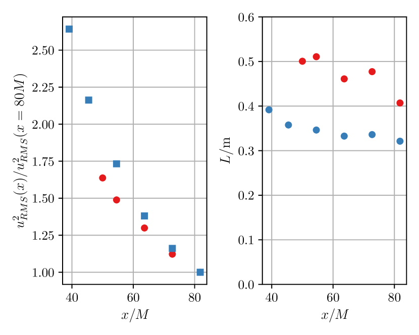
Figure 6: Development of the turbulent kinetic energy (left) and integral length scale $L$ (right) for different distances from the active grid. The distances are normalised by the active grid paddle dimensions. $L$ was estimated using $\int_{0}^{r_{0}}\!C_{11}(r)/u_{RMS}^{2}\,dr$ with $r_{0}$ the first zero-crossing of the correlation function.

A.2 Measurement Technology and Data Analysis

We record time series of hot-wire signals and convert them into one-dimensional flow fields assuming that the turbulent fluctuations are passively advected across the sensor by the mean flow $U$. Thus, a time step $\Delta t$ is converted to a spatial increment $\Delta x=U\Delta t$ [4]. We use a commercial constant temperature anemometer (Dantec StreamWare) to drive and acquire data from Nanoscale Thermal Anemometry Probes (NSTAP) provided by Princeton University [67, 68, 69]. These ultra-small hot wire probes average the flow field over a length of only 30 $\mu$m, which is sufficient for this experiment. For flows where the viscous length scales are larger, we also use commercial hot wires from Dantec Dynamics with sensing length 450 $\mu$m ($\gtrsim 4\eta$). The probe length is indicated by dotted vertical lines in Fig. 7 and far away from the region of interest.

To achieve converged statistics the data was acquired for $10^{3}$ - $10^{4}$ eddy turnover times (up to 8 hours) between $150<R_{\lambda}<6000$.

The frequencies (and wavenumbers) encountered in the measurements presented here are generally in a range that is not particularly demanding for this combination of sensor and anemometer circuitry [70, 71, 72]. The temporal resolution is determined by the noise filtering frequency and the frequency response of the measurement system. The frequency response of the system is not perfectly flat anymore starting around 1 kHz [70]. The range of scales we are interested in is therefore in the flat part of the frequency response curve. To illustrate this, the length scales corresponding to a measurement frequency of 1 kHz are indicated in Fig. 7 as vertical lines in the color of the corresponding $\zeta_{2}(r)$. The noise filtering frequency is always at frequencies above 1kHz.

The experiments presented here were taken under different ambient pressures and different active grid forcing schemes to allow for a careful check of the hot wire fidelity. We thus ensure the robustness of the results against probe- or flow geometry-induced biases. We emphasise that all conclusions presented here are independent of the frequencies where turbulent fluctuations are measured, the dissipation length scale, and the active grid forcing.

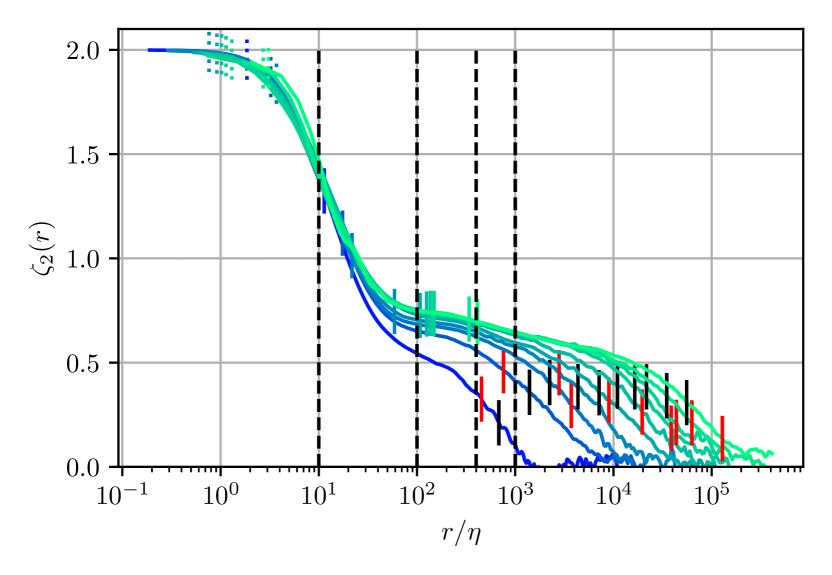
Figure 7: Same as Fig. 1 (A) with the addition of probe length (dotted vertical lines), the value of $r/\eta$ corresponding to a measurement frequency of 1 kHz through Taylor’s Hypothesis (vertical lines), the values of $r_{0}/\eta$ chosen to assemble Fig. 1 (D) (dashed black lines), the length of the energy injection scale (vertical black lines), and the grid length scale (red lines).

A.3 Fits to the Model Spectrum [28]

The evolution equation of the velocity energy spectrum $E(k,t)$ can be derived directly from the Navier-Stokes-Equation in the isotropic case and is known as the Karman-Howarth-Lin equation.

$$\partial_{t}E(k,t)=-\partial_{k}\Pi(k,t)-2\nu k^{2}E(k,t).$$ (7)

The first term on the RHS describes the nonlinear transfer of energy from small to large wavenumbers and ultimately prevents the closure of the equation, since it is a third-order term. The Pao closure [73] used in the model by Yang et al. [28] assumes that the transfer term $\Pi$ is local in wavenumber space and has a self-similar form:

$$\Pi(k,t)=C_{0}\varepsilon^{1/3}k^{5/3}E(k,t)$$ (8)

The second term on the RHS of (7) represents the viscous dissipation at the smallest flow scales. This yields a closed form of the Karman-Howarth-Lin equation. The model by Yang et al. further assumes that the energy spectrum can be assembled by a large scale term $f_{L}(kL)$, a small scale term $f_{\eta}(k\eta)$, and a self-similar inertial range:

$$E(k,t)=C_{k}\varepsilon^{2/3}k^{5/3}f_{\eta}(k\eta)f_{L}(kL)$$ (9)

These assumptions are now combined with a general, self-similar decay of turbulent kinetic energy. In the case of a confined domain, where the parameter describing $dL/dt$ tends to zero, this model predicts the energy spectrum

$$E(k)\sim\frac{-A_{K}}{C}(kL)^{-(\zeta_{2F}+1)}e^{(3A_{K}/2C)(kL)^{-2/3}}e^{-(1.5/C)(k\eta)^{4/3}}.$$ (10)

For the purpose of measuring a scaling exponent, we replaced the term $(kL)^{-5/3}$ used in the original formulation of the spectrum with $(kL)^{-(\zeta_{2F}+1)}$, where the fitting parameter $\zeta_{2F}$ is the inertial range scaling exponent for the second order structure function[74]. The parameters $C$ and $A_{K}$ are related through $C=-A_{K}(6/\pi)^{1/3}$. In practice, $A_{K}$ describes the large-scale part of the energy spectrum, which is heavily influenced by the decay.

The one-dimensional versions of $S_{2}$ and $E(k)$ are related through the following integral transform [75]:

$$S_{2}(r)=\int_{0}^{\infty}\!E(k)\left(\frac{1}{3}+\frac{\cos(kr)}{(kr)^{2}}-\frac{\sin(kr)}{(kr)^{3}}\right)dk.$$ (11)

To obtain the fits shown in Fig. 4, we have searched for parameters $A_{K}$, and $\zeta_{2F}$ that yield best fits of the logarithmic derivative of eq. (11) to the experimentally measured $\zeta_{2}(r)$.

It can be shown that $C=-A_{K}(6/\pi)^{1/3}$. This quantity is related to the dissipation constant $C_{\varepsilon}=\varepsilon L/u^{3}$ relating the large scale energy injection and the small scale energy transfer rate $\varepsilon$. $A_{K}$ is the non-dimensionalized time-evolution of the energy spectrum prefactor $d(C_{K}\varepsilon^{2/3})/dt$, which is a free parameter.

The energy transfer spectrum $\Pi(k)$ is related to $S_{3}$ via

$$S_{3}=12\int_{0}^{\infty}\!\frac{1}{k^{2}}\frac{\partial\Pi}{\partial k}\frac{d}{dr}\left(\frac{1}{3}+\frac{\cos(kr)}{(kr)^{2}}-\frac{\sin(kr)}{(kr)^{3}}\right)dk.$$ (12)

The second derivative has been estimated by a Taylor expansion for $kr<0.001$. Therefore, the model (10) in combination with its underlying closure hypothesis eq. (9) implicitly predicts $S_{3}$. Note that strictly speaking the combination of the intermittency-corrected model eq. (10) and the K41-type closure eq. (9) yields a third order exponent $\zeta_{3}$ slightly different from 1. It is reassuring to see that instead leaving the 5/3-term in eq. (9) as a generic scaling and fitting the resulting model to $S_{3}$ yields $\Pi\approx$ const. in the inertial range so that $S_{3}\sim r$.

A.4 Dependence of $F_{2}$ on $\mu_{2}$

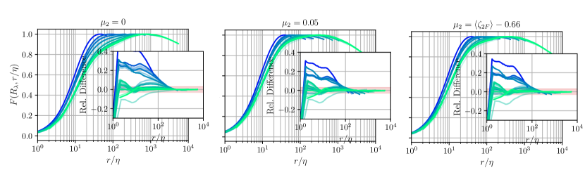
Figure 8: $F_{2}$ for different values of $\mu_{2}$. The K41 estimate $0.66$ provides the least degree of universality. No substantial differences appear in the most likely range of $\mu_{2}$ between 0.69 and 0.71.

The precise form of $F_{2}(R_{\lambda},r/\eta)$ depends on the choice of $\mu_{2}$, which is subject to systematic and statistical measurement errors. A poor estimate of $\mu_{2}$ might thus distort $F_{2}$ and disguise departures from universality of this function. We have recomputed the lower plot of Fig. 5 for different values of $\mu_{2}$ and present the results in Fig. 8. $F_{2}$ does not vary noticably for exemplary values of $\mu_{2}$ within the most likely true range. It becomes clear that the K41 prediction $\mu=0$ does not produce a universal form of $F_{2}$, which is expected in the light of the vast evidence in favour of intermittency corrections. Values of $\mu$ within its likely range between 0.68 and 0.71 yield very similar values of $F_{2}$. Most importantly its universality is not impacted significantly.

References

- Bodenschatz et al. [2014a] E. Bodenschatz, G. P. Bewley, H. Nobach, M. Sinhuber, and H. Xu, Variable density turbulence tunnel facility, Review of Scientific Instruments 85, 093908 (2014a).
- Griffin et al. [2019] K. P. Griffin, N. J. Wei, E. Bodenschatz, and G. P. Bewley, Control of long-range correlations in turbulence, Experiments in Fluids 60, 55 (2019), arXiv:1809.05126 .
- Kolmogorov [1941] A. N. Kolmogorov, The Local Structure of Turbulence in Incompressible Viscous Fluid for Very Large Reynolds Numbers, Proceedings: Mathematical and Physical Sciences 434, 9 (1941).
- Taylor [1935] G. I. Taylor, Statistical theory of turbulenc, Proceedings of the Royal Society A: Mathematical, Physical and Engineering Sciences 151, 421 (1935).
- Ishihara et al. [2020] T. Ishihara, Y. Kaneda, K. Morishita, M. Yokokawa, and A. Uno, Second-order velocity structure functions in direct numerical simulations of turbulence with up to 2250, Phys. Rev. Fluids 5, 104608 (2020).
- Tsuji [2004a] Y. Tsuji, Intermittency effect on energy spectrum in high-Reynolds number turbulence, Physics of Fluids 16, L43 (2004a).
- Meyers and Baelmans [2004] J. Meyers and M. Baelmans, Determination of subfilter energy in large-eddy simulations, Journal of Turbulence 5, N26 (2004).
- Batchelor and Townsend [1947] G. K. Batchelor and A. Townsend, Decay of vorticity in isotropic turbulence, Proceedings of the Royal Society of London. Series A. Mathematical and Physical Sciences 190, 534 (1947).
- G. K. Batchelor and Townsend, A.A. [1949] G. K. Batchelor and Townsend, A.A., The nature of turbulent motion at large wave-numbers, Proceedings of the Royal Society of London. Series A. Mathematical and Physical Sciences 199, 238 (1949).
- Kolmogorov [1962] A. N. Kolmogorov, A refinement of previous hypotheses concerning the local structure of turbulence in a viscous incompressible fluid at high Reynolds number, Journal of Fluid Mechanics 13, 82 (1962).
- Frisch et al. [1978] U. Frisch, P.-L. Sulem, and M. Nelkin, A simple dynamical model of intermittent fully developed turbulence, Journal of Fluid Mechanics 87, 719 (1978).
- Benzi et al. [1984] R. Benzi, G. Paladin, G. Parisi, and A. Vulpiani, On the multifractal nature of fully developed turbulence and chaotic systems, Journal of Physics A: Mathematical and General 17, 3521 (1984).
- Sreenivasan and Meneveau [1986] K. R. Sreenivasan and C. Meneveau, The fractal facets of turbulence, Journal of Fluid Mechanics 173, 357 (1986).
- Meneveau and Sreenivasan [1987] C. Meneveau and K. R. Sreenivasan, Simple multifractal cascade model for fully developed turbulence, Physical Review Letters 59, 1424 (1987).
- Andrews et al. [1989] L. C. Andrews, R. L. Phillips, B. K. Shivamoggi, J. K. Beck, and M. L. Joshi, A statistical theory for the distribution of energy dissipation in intermittent turbulence, Physics of Fluids A: Fluid Dynamics 1, 999 (1989).
- She and Leveque [1994] Z.-S. She and E. Leveque, Universal scaling laws in fully developed turbulence, Physical Review Letters 72, 336 (1994).
- Dubrulle [1994] B. Dubrulle, Intermittency in fully developed turbulence: Log-Poisson statistics and generalized scale covariance, Physical Review Letters 73, 959 (1994).
- Barenblatt and Goldenfeld [1995] G. I. Barenblatt and N. Goldenfeld, Does fully developed turbulence exist? Reynolds number independence versus asymptotic covariance, Physics of Fluids 7, 3078 (1995).
- Praskovsky and Oncley [1994] A. Praskovsky and S. Oncley, Measurements of the Kolmogorov constant and intermittency exponent at very high Reynolds numbers, Physics of Fluids 6, 2886 (1994).
- Sreenivasan [1998] K. R. Sreenivasan, An update on the energy dissipation rate in isotropic turbulence, Physics of Fluids 10, 528 (1998).
- Kahalerras et al. [1998] H. Kahalerras, Y. Malécot, Y. Gagne, and B. Castaing, Intermittency and Reynolds number, Physics of Fluids 10, 910 (1998).
- Tsuji [2004b] Y. Tsuji, Intermittency effect on energy spectrum in high-Reynolds number turbulence, Physics of Fluids 16, L43 (2004b).
- White et al. [2002] C. M. White, A. N. Karpetis, and K. R. Sreenivasan, High-Reynolds-number turbulence in small apparatus: Grid turbulence in cryogenic liquids, Journal of Fluid Mechanics 452, 189 (2002).
- Pietropinto et al. [2003] S. Pietropinto, C. Poulain, C. Baudet, B. Castaing, B. Chabaud, Y. Gagne, B. Hébral, Y. Ladam, P. Lebrun, O. Pirotte, and P. Roche, Superconducting instrumentation for high Reynolds turbulence experiments with low temperature gaseous helium, Physica C: Superconductivity 386, 512 (2003).
- Bewley and Sreenivasan [2009] G. P. Bewley and K. R. Sreenivasan, The Decay of a Quantized Vortex Ring and the Influence of Tracer Particles, Journal of Low Temperature Physics 156, 84 (2009).
- Salort et al. [2012] J. Salort, B. Chabaud, E. Lévêque, and P.-E. Roche, Energy cascade and the four-fifths law in superfluid turbulence, EPL (Europhysics Letters) 97, 34006 (2012).
- Rousset et al. [2014] B. Rousset, P. Bonnay, P. Diribarne, A. Girard, J. M. Poncet, E. Herbert, J. Salort, C. Baudet, B. Castaing, L. Chevillard, F. Daviaud, B. Dubrulle, Y. Gagne, M. Gibert, B. Hébral, T. Lehner, P.-E. Roche, B. Saint-Michel, and M. Bon Mardion, Superfluid high REynolds von Kármán experiment, Review of Scientific Instruments 85, 103908 (2014).
- Yang et al. [2018] P.-F. Yang, A. Pumir, and H. Xu, Generalized self-similar spectrum and the effect of large-scale in decaying homogeneous isotropic turbulence, New Journal of Physics 20, 103035 (2018).
- Saddoughi and Veeravalli [1994] S. G. Saddoughi and S. V. Veeravalli, Local isotropy in turbulent boundary layers at high Reynolds number, Journal of Fluid Mechanics 268, 333 (1994).
- Mydlarski and Warhaft [1996] L. Mydlarski and Z. Warhaft, On the onset of high-Reynolds-number grid-generated wind tunnel turbulence, Journal of Fluid Mechanics 320, 331 (1996).
- Antonia et al. [2019] R. A. Antonia, S. L. Tang, L. Djenidi, and Y. Zhou, Finite Reynolds number effect and the 4/5 law, Physical Review Fluids 4, 084602 (2019).
- Sinhuber et al. [2017] M. Sinhuber, G. P. Bewley, and E. Bodenschatz, Dissipative Effects on Inertial-Range Statistics at High Reynolds Numbers, Physical Review Letters 119, 134502 (2017).
- Küchler et al. [2019] C. Küchler, G. P. Bewley, and E. Bodenschatz, Experimental Study of the Bottleneck in Fully Developed Turbulence, Journal of Statistical Physics 175, 617 (2019), arXiv:1812.01370 .
- Fukayama et al. [2000] D. Fukayama, T. Oyamada, T. Nakano, T. Gotoh, and K. Yamamoto, Longitudinal Structure Functions in Decaying and Forced Turbulence, Journal of the Physical Society of Japan 69, 701 (2000), arXiv:chao-dyn/9912033 .
- Gotoh et al. [2002] T. Gotoh, D. Fukayama, and T. Nakano, Velocity field statistics in homogeneous steady turbulence obtained using a high-resolution direct numerical simulation, Physics of Fluids 14, 1065 (2002).
- Chen et al. [2005] S. Y. Chen, B. Dhruva, S. Kurien, K. R. Sreenivasan, and M. A. Taylor, Anomalous scaling of low-order structure functions of turbulent velocity, Journal of Fluid Mechanics 533, 10.1017/S002211200500443X (2005).
- Tang et al. [2017] S. L. Tang, R. A. Antonia, L. Djenidi, L. Danaila, and Y. Zhou, Finite Reynolds number effect on the scaling range behaviour of turbulent longitudinal velocity structure functions, Journal of Fluid Mechanics 820, 341 (2017).
- Yeung et al. [2018] P. K. Yeung, K. R. Sreenivasan, and S. B. Pope, Effects of finite spatial and temporal resolution in direct numerical simulations of incompressible isotropic turbulence, Physical Review Fluids 3, 064603 (2018).
- Danaila et al. [2002] L. Danaila, F. Anselmet, and R. A. Antonia, An overview of the effect of large-scale inhomogeneities on small-scale turbulence, Physics of Fluids 14, 2475 (2002).
- Antonia et al. [2015] R. A. Antonia, S. L. Tang, L. Djenidi, and L. Danaila, Boundedness of the velocity derivative skewness in various turbulent flows, Journal of Fluid Mechanics 781, 727 (2015).
- Bos et al. [2012] W. J. T. Bos, L. Chevillard, J. F. Scott, and R. Rubinstein, Reynolds number effect on the velocity increment skewness in isotropic turbulence, Physics of Fluids 24, 015108 (2012).
- [42] T. de Karman and L. Howarth, On the Statistical Theory of Isotropic Turbulence, 164, 192.
- Antonia et al. [2003] R. A. Antonia, R. J. Smalley, T. Zhou, F. Anselmet, and L. Danaila, Similarity of energy structure functions in decaying homogeneous isotropic turbulence, Journal of Fluid Mechanics 487, 245 (2003).
- [44] L. Danaila, F. Anselmet, T. Zhou, and R. A. Antonia, A generalization of Yaglom’s equation which accounts for the large-scale forcing in heated decaying turbulence, 391, 359.
- Antonia and Burattini [2006] R. A. Antonia and P. Burattini, Approach to the 4/5 law in homogeneous isotropic turbulence, Journal of Fluid Mechanics 550, 175 (2006).
- Thiesset et al. [2013] F. Thiesset, R. A. Antonia, L. Danaila, and L. Djenidi, Kármán-Howarth closure equation on the basis of a universal eddy viscosity, Physical Review E 88, 011003 (2013).
- Batchelor [1951] G. K. Batchelor, Pressure fluctuations in isotropic turbulence, Mathematical Proceedings of the Cambridge Philosophical Society 47, 359 (1951).
- Lohse and Müller-Groeling [1995] D. Lohse and A. Müller-Groeling, Bottleneck Effects in Turbulence: Scaling Phenomena in r versus p Space, Physical Review Letters 74, 1747 (1995).
- Kurien and Sreenivasan [2000a] S. Kurien and K. R. Sreenivasan, Anisotropic scaling contributions to high-order structure functions in high-Reynolds-number turbulence, Physical Review E 62, 2206 (2000a).
- Dhruva [2000] B. R. Dhruva, An experimental study of high Reynolds number turbulence in the atmosphere, Ph.D. Thesis , 2717 (2000).
- Meyers and Meneveau [2008] J. Meyers and C. Meneveau, A functional form for the energy spectrum parametrizing bottleneck and intermittency effects, Physics of Fluids 20, 065109 (2008).
- Antonia [1982] R. A. Antonia, Reynolds number dependence of velocity structure functions in turbulent shear flows, Physics of Fluids 25, 29 (1982).
- Tang et al. [2019] S. Tang, R. A. Antonia, L. Djenidi, and Y. Zhou, Can small-scale turbulence approach a quasi-universal state?, Physical Review Fluids 4, 024607 (2019).
- Vallikivi et al. [2011] M. Vallikivi, M. Hultmark, S. C. C. Bailey, and A. J. Smits, Turbulence measurements in pipe flow using a nano-scale thermal anemometry probe, Experiments in Fluids 51, 1521 (2011).
- Saffman [1967] P. G. Saffman, The large-scale structure of homogeneous turbulence, Journal of Fluid Mechanics 27, 581 (1967).
- Sinhuber et al. [2015] M. Sinhuber, E. Bodenschatz, and G. P. Bewley, Decay of Turbulence at High Reynolds Numbers, Physical Review Letters 114, 034501 (2015).
- Benzi et al. [1993] R. Benzi, S. Ciliberto, R. Tripiccione, C. Baudet, F. Massaioli, and S. Succi, Extended self-similarity in turbulent flows, Physical Review E 48, R29 (1993).
- Kurien and Sreenivasan [2000b] S. Kurien and K. R. Sreenivasan, Anisotropic scaling contributions to high-order structure functions in high-Reynolds-number turbulence, Physical Review E 62, 2206 (2000b).
- Biferale and Procaccia [2005] L. Biferale and I. Procaccia, Anisotropy in Turbulent Flows and in Turbulent Transport, Physics Reports 414, 43 (2005), arXiv:nlin/0404014 .
- Iyer et al. [2020] K. P. Iyer, K. R. Sreenivasan, and P. K. Yeung, Scaling exponents saturate in three-dimensional isotropic turbulence, Physical Review Fluids 5, 054605 (2020).
- Brasseur and Wei [1994] J. G. Brasseur and C. Wei, Interscale dynamics and local isotropy in high reynolds number turbulence within triadic interactions, Physics of Fluids 6, 842 (1994), https://doi.org/10.1063/1.868322 .
- Alexakis et al. [2005] A. Alexakis, P. D. Mininni, and A. Pouquet, Imprint of large-scale flows on turbulence, Phys. Rev. Lett. 95, 264503 (2005).
- Verma and Donzis [2007] M. K. Verma and D. Donzis, Energy Flux and Bottleneck Effect in Turbulence, arXiv:nlin/0510026 10.1088/1751-8113/40/16/010 (2007), arXiv:nlin/0510026 .
- Leung et al. [2012] T. Leung, N. Swaminathan, and P. A. Davidson, Geometry and interaction of structures in homogeneous isotropic turbulence, Journal of Fluid Mechanics 710, 453 (2012).
- Bodenschatz et al. [2014b] E. Bodenschatz, G. P. Bewley, H. Nobach, M. Sinhuber, and H. Xu, Variable Density Turbulence Tunnel Facility, Review of Scientific Instruments 85, 093908 (2014b), arXiv:1401.4970 .
- Davidson [2015] P. Davidson, Turbulence: An Introduction for Scientists and Engineers (Oxford University Press, 2015).
- Kunkel et al. [2006] G. Kunkel, C. Arnold, and A. Smits, Development of NSTAP: Nanoscale Thermal Anemometry Probe, in 36th AIAA Fluid Dynamics Conference and Exhibit (American Institute of Aeronautics and Astronautics, San Francisco, California, 2006).
- Vallikivi and Smits [2014] M. Vallikivi and A. J. Smits, Fabrication and Characterization of a Novel Nanoscale Thermal Anemometry Probe, Journal of Microelectromechanical Systems 23, 899 (2014).
- Fan et al. [2015] Y. Fan, G. Arwatz, T. W. Van Buren, D. E. Hoffman, and M. Hultmark, Nanoscale sensing devices for turbulence measurements, Experiments in Fluids 56, 138 (2015).
- Hutchins et al. [2015] N. Hutchins, J. P. Monty, M. Hultmark, and A. J. Smits, A direct measure of the frequency response of hot-wire anemometers: Temporal resolution issues in wall-bounded turbulence, Experiments in Fluids 56, 18 (2015).
- Samie et al. [2018] M. Samie, N. Hutchins, and I. Marusic, Revisiting end conduction effects in constant temperature hot-wire anemometry, Experiments in Fluids 59, 133 (2018).
- Ashok et al. [2012] A. Ashok, S. C. C. Bailey, M. Hultmark, and A. J. Smits, Hot-wire spatial resolution effects in measurements of grid-generated turbulence, Experiments in Fluids 53, 1713 (2012).
- Pao [1965] Y.-H. Pao, Structure of Turbulent Velocity and Scalar Fields at Large Wavenumbers, Physics of Fluids 8, 1063 (1965).
- Pope and Pope [2000] S. B. Pope and S. B. Pope, Turbulent Flows (Cambridge University Press, 2000).
- Monin and Yaglom [1975] A. S. Monin and A. Yaglom, Statistical Fluid Mechanics: Mechanics of Turbulence. 2 2, edited by J. L. Lumley (MIT Pr., Cambridge, Mass., 1975).