The solar-wind angular-momentum flux observed during Solar Orbiter’s first orbit

Abstract

Aims. We present the first measurements of the solar-wind angular-momentum flux recorded by the Solar Orbiter spacecraft. Our aim is the validation of these measurements to support future studies of the Sun’s angular-momentum loss.

Methods. We combine 60-minute averages of the proton bulk moments and the magnetic field measured by the Solar Wind Analyser (SWA) and the magnetometer (MAG) onboard Solar Orbiter. We calculate the angular-momentum flux per solid-angle element using data from the first orbit of the mission’s cruise phase during 2020. We separate the contributions from protons and from magnetic stresses to the total angular-momentum flux.

Results. The angular-momentum flux varies significantly over time. The particle contribution typically dominates over the magnetic-field contribution during our measurement interval. The total angular-momentum flux shows the largest variation and is typically anti-correlated with the radial solar-wind speed. We identify a compression region, potentially associated with a co-rotating interaction region or a coronal mass ejection, that leads to a significant localised increase in the angular-momentum flux, yet without a significant increase in the angular momentum per unit mass. We repeat our analysis using the density estimate from the Radio and Plasma Waves (RPW) instrument. Using this independent method, we find a decrease in the peaks of positive angular-momentum flux but otherwise consistent results.

Conclusions. Our results largely agree with previous measurements of the solar-wind angular-momentum flux in terms of amplitude, variability, and dependence on radial solar-wind bulk speed. Our analysis highlights the potential for future, more detailed, studies of the solar wind’s angular momentum and its other large-scale properties with data from Solar Orbiter. We emphasise the need to study the radial evolution and latitudinal dependence of the angular-momentum flux in combination with data from Parker Solar Probe and assets at heliocentric distances of 1 au and beyond.

1 Introduction

The solar corona expands into interplanetary space in the form of the solar wind (Parker, 1958; Neugebauer & Snyder, 1962; Verscharen et al., 2019). In this process, the solar-wind plasma removes mass, momentum, energy, and angular momentum from the Sun. In the lower corona, the Sun’s magnetic field forces the plasma into a quasi-rigid co-rotation with the photosphere, following the co-rotation of the field’s photospheric footpoints. With increasing distance from the photosphere, the torque exerted by the coronal magnetic field on the plasma decreases (Weber & Davis, 1967). In this way, the large-scale magnetic field mediates a smooth transition from co-rotation to quasi-radial expansion. Therefore, the solar wind is not “flung” from the photosphere on a ballistic trajectory, which would lead to a torque-free azimuthal velocity profile of the form

$$U_{\phi}(r)\simeq\frac{R_{\odot}^{2}\Omega_{\odot}\sin\theta}{r},$$ (1)

where $R_{\odot}$ is the solar radius, $\Omega_{\odot}$ is the Sun’s angular rotation frequency, $\theta$ is the co-latitude, and $r$ is the heliocentric distance. Instead, the solar wind experiences a significant torque in its acceleration region at even larger distances from the photosphere, leading to greater azimuthal speeds than predicted by Eq. (1). In turn, the torque applied to the Sun by the magnetic field in this process slows down the Sun’s rotation on long time scales (Mestel, 1968; Reiners & Mohanty, 2012). Local measurements of the solar-wind angular-momentum flux provide an estimate for the global angular-momentum loss rate, which ultimately causes the rotation period of the Sun and, by extrapolation, of Sun-like stars on the main sequence to increase with age (Barnes, 2003; Gallet & Bouvier, 2013; Matt et al., 2015; Pantolmos & Matt, 2017).

Measurements of the solar-wind angular-momentum flux are particularly challenging from an instrumental point of view. They require an accurate determination of the azimuthal component $U_{\phi}$ of the particle bulk velocity, which is typically more than one order of magnitude less than its radial component $U_{r}$. Nevertheless, early measurements of the solar wind already estimated its angular momentum (Hundhausen et al., 1970; Lazarus & Goldstein, 1971; Pizzo et al., 1983; Marsch & Richter, 1984). Modern space instrumentation provides us with higher spacecraft-pointing accuracy and thus a more accurate determination of $U_{\phi}$. Moreover, as the average ratio $U_{\phi}/U_{r}$ increases with decreasing heliocentric distance, the error in the quantification of the angular-momentum flux is generally smaller when measured at smaller distances from the Sun (Finley et al., 2020, 2021). In addition, co-rotating interaction regions have not yet formed (Richter & Luttrell, 1986; Allen et al., 2020), and interplanetary coronal mass ejections have not fully expanded to disturb nearby wind streams (Möstl et al., 2020) at small distances from the Sun. Therefore, near-Sun measurements enable the sampling of more pristine and less processed solar wind. Solar Orbiter and Parker Solar Probe share the advantages of both modern space instrumentation and an orbit that leads them close to the Sun (Fox et al., 2016; Müller et al., 2020). We present the first observations of the solar wind’s angular-momentum flux observed by Solar Orbiter during the first orbit of its cruise phase in 2020.

2 Data analysis

We analyse a combined set of data from the Proton-Alpha Sensor (PAS) of Solar Orbiter’s Solar Wind Analyser (SWA, Owen et al., 2020) suite and from Solar Orbiter’s fluxgate magnetometer (MAG, Horbury et al., 2020). Our dataset includes all time intervals from 2020-07-07 until 2020-10-27, for which both SWA/PAS and MAG data are available. We ignore all other intervals and those in which the quality flags for either dataset indicate poor data quality (we only include data with a quality flag of 3). After this selection, we thus retain about 38.9% of the total time interval in our dataset (for time coverage, see also Figure 1). During this time, Solar Orbiter recorded data at heliocentric distances between 0.591 and 0.989 au. The time average of the spacecraft’s heliocentric distance in our dataset is 0.851 au.

The calculation of the angular-momentum flux is very sensitive to knowledge uncertainties in the direction of the bulk velocity and in the direction of the magnetic field. The finite angular resolution of PAS introduces an uncertainty in the knowledge of the bulk-speed direction. The calibration accuracy of PAS is $\lesssim 1^{\circ}$. The pointing knowledge of the MAG sensor is largely determined by the uncertainty of the spacecraft’s boom deployment angle. It introduces an angular uncertainty of the magnetic-field measurement of $\lesssim 1^{\circ}$. Planned inter-instrument alignment reconstructions of the boom orientation will become feasible in the future once the instruments have recorded sufficient amounts of data for a large statistical analysis (Walsh et al., 2020). For solar-wind speeds above $300\,\mathrm{km\,s}^{-1}$, the relative uncertainty of the SWA/PAS speed measurement due to counting statistics is less than 1%. The relative uncertainty of the density measurement is energy-dependent with a maximum of 20%, which we apply as a conservative estimate to our entire dataset. At very low energies (corresponding to solar-wind speeds below $\sim 300\,\mathrm{km\,s}^{-1}$), the sensitivity decreases further so that additional correction factors are required, which have not been conclusively determined yet. The expected MAG offset is $\sim\pm 0.1\,\mathrm{nT}$, which we take as the absolute uncertainty of our individual magnetic-field component measurements. The requirement of the absolute knowledge error of the spacecraft pointing is $\leq 3\,\mathrm{arcmin}$ (García Marirrodriga et al., 2021), which is mostly driven by the instrument requirements of the remote-sensing suite and a minor contributor to the pointing knowledge uncertainties for our study.

We base our analysis on the PAS normal-mode ground moments integrated from the proton part (core and beam) of the full three-dimensional measured ion distributions and the MAG normal-mode vectors of the magnetic field. In normal mode, the PAS ground moments are available every 4 seconds, while the MAG vectors are available with a cadence of 8 vectors per second. We merge and average both data products over intervals of length 60 min to reduce natural fluctuations in the data due to, for example, waves and turbulence, as we are interested in the angular-momentum flux of the bulk solar wind. Our selection and averaging procedure leaves us with 1036 individual data points.

The angular momentum is contained in the mechanical flux of the solar-wind particles. In addition, there is transport of angular momentum due to magnetic-field stresses. Ignoring anisotropies in the particle distributions and contributions from particles other than protons, the total angular-momentum flux is thus the sum of the proton and magnetic-field terms (see Marsch & Richter, 1984). We define the total angular-momentum flux per solid-angle element in spherical heliocentric coordinates as

$$\mathcal{F}_{\mathrm{tot}}=\mathcal{F}_{\mathrm{p}}+\mathcal{F}_{B},$$ (2)

where

$$\mathcal{F}_{\mathrm{p}}=r^{3}\rho U_{r}U_{\phi}$$ (3)

is the proton contribution to the angular-momentum flux,

$$\mathcal{F}_{B}=-r^{3}\frac{B_{r}B_{\phi}}{4\pi}$$ (4)

is the contribution from magnetic stresses (in cgs units) to the angular-momentum flux, $r$ is the heliocentric distance, $\rho$ is the proton mass density, $\@vec{U}$ is the proton bulk velocity, and $\@vec{B}$ is the magnetic field. The subscript $r$ indicates the radial vector component, and the subscript $\phi$ indicates the azimuthal component in spherical heliocentric coordinates. We use our 60-minute averages of the measured solar-wind parameters as the input for our calculations of $\mathcal{F}_{\mathrm{p}}$ and $\mathcal{F}_{B}$ according to Equations (3) and (4). We recognise that our analysis represents only a first validation of methods to study angular-momentum flux with Solar Orbiter. Therefore, it ignores other contributions to the total angular-momentum flux (see Section 4), which must be investigated in future detailed studies.

3 Results

3.1 Timeseries and overview

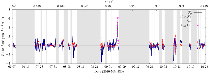
Figure 1: Timeseries of the angular-momentum flux per solid-angle element measured during Solar Orbiter’s first orbit of the cruise phase. The diagram shows the proton contribution $\mathcal{F}_{\mathrm{p}}$, the magnetic-field contribution $\mathcal{F}_{B}$ and the sum of both, $\mathcal{F}_{\mathrm{tot}}$. In order to increase the visibility, we multiply $\mathcal{F}_{B}$ with a factor 10. The magenta squares represent the measurements of $\mathcal{F}_{\mathrm{tot}}$ during the time of the compression region (CR) on 2020-09-06. The axis at the top indicates the heliocentric distance of the spacecraft at the time of the measurement. The scale of this axis is not linear. The grey-shaded areas indicate times for which our merged SWA/PAS-MAG data product is unavailable or the data flags for either dataset indicate poor data quality.

Figure 1 shows the timeseries of $\mathcal{F}_{\mathrm{p}}$, $\mathcal{F}_{B}$, and $\mathcal{F}_{\mathrm{tot}}$ over the analysed data interval. Gaps in this plot represent data gaps or those intervals that we exclude according to our selection criteria. Figure 1 illustrates the natural variation of the angular-momentum flux over time, which is typically greater than its mean magnitude. Across all data points, the mean value of $\mathcal{F}_{\mathrm{p}}$ is $2.29\times 10^{-11}\,\mathrm{au}^{3}\,\mathrm{g\,cm}^{-1}\,\mathrm{s}^{-2}\,\mathrm{sr}^{-1}$, while the mean value of $\mathcal{F}_{B}$ is $1.72\times 10^{-11}\,\mathrm{au}^{3}\,\mathrm{g\,cm}^{-1}\,\mathrm{s}^{-2}\,\mathrm{sr}^{-1}$. In general, $\mathcal{F}_{\mathrm{p}}$ exhibits significantly more variation than $\mathcal{F}_{B}$. As expected for a conserved quantity, $\mathcal{F}_{\mathrm{tot}}$ shows no secular dependence on heliocentric distance.

On 2020-09-06, we record a time interval of significantly increased $\mathcal{F}_{\mathrm{p}}$ and $\mathcal{F}_{\mathrm{tot}}$. Upon closer inspection, this interval corresponds to a time of increased $\rho$, probably associated with the compression in front of a co-rotating interaction region or a coronal mass ejection seen as a flux rope in the magnetic field. Due to this enhancement in $\rho$, the associated plasma carries more angular-momentum flux than the solar wind before or after the compression region. The compression region does not exhibit enhancements in $U_{r}$ or $U_{\phi}$ (not shown here), suggesting that the compression region facilitates a similar angular-momentum flux per unit mass as the solar wind. Figure 6 supports this suggestion as discussed below. We highlight the measurements taken during the time interval associated with this compression region in our figures as magenta squares.

3.2 Variability of the angular-momentum flux

In Figures 2 and 3, we show histograms of the measured values of $\mathcal{F}_{\mathrm{p}}$ and $\mathcal{F}_{B}$ in our dataset in terms of their probability distributions. We colour-code the contributions from fast, intermediate, and slow solar wind in our histograms. Due to the dominance of $\mathcal{F}_{\mathrm{p}}$, the histogram of the probability distribution for $\mathcal{F}_{\mathrm{tot}}$ (not shown) is almost identical with the histogram for $\mathcal{F}_{\mathrm{p}}$. Both histograms reflect the large variation in the angular-momentum flux and the range of observed values. According to Figure 2, the majority distribution is centred around negative values of $\mathcal{F}_{\mathrm{p}}$, while the outliers at large $\mathcal{F}_{\mathrm{p}}$ shift the mean of our measurements to $\mathcal{F}_{\mathrm{p}}>0$. These outliers are mostly associated with the compression region on 2020-09-06.

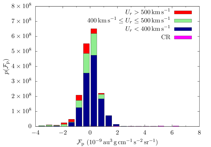
Figure 2: Histogram of the proton contribution $\mathcal{F}_{\mathrm{p}}$ to the solar wind’s angular-momentum flux per solid-angle element. The vertical axis indicates the probability density of $\mathcal{F}_{\mathrm{p}}$. We stack the histograms for fast ($U_{r}>500\,\mathrm{km\,s}^{-1}$), intermediate ($400\,\mathrm{km\,s}^{-1}\leq U_{r}\leq 500\,\mathrm{km\,s}^{-1}$), and slow ($U_{r}<400\,\mathrm{km\,s}^{-1}$) wind. The magenta areas represent the measurements of $\mathcal{F}_{\mathrm{p}}$ during the time of the compression region (CR) on 2020-09-06.

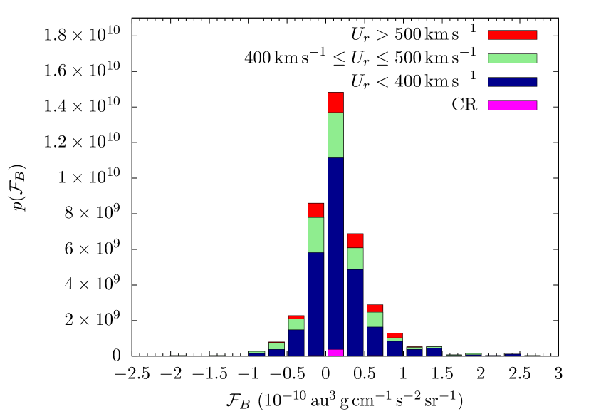
Figure 3: Same as Figure 2, but for the magnetic-field contribution $\mathcal{F}_{B}$ to the solar wind’s angular-momentum flux per solid-angle element.

For a more quantitative statistical analysis, we list the mean values, the standard deviations, as well as the maximum and minimum values of $\mathcal{F}_{\mathrm{p}}$, $\mathcal{F}_{B}$, and $\mathcal{F}_{\mathrm{tot}}$ in Table 1. In addition, Table 1 provides these statistical markers separated by time intervals with $U_{r}<400\,\mathrm{km\,s}^{-1}$ and $U_{r}>500\,\mathrm{km\,s}^{-1}$ as a means to distinguish characteristic slow wind from fast wind, respectively. We find that $\mathcal{F}_{\mathrm{p}}>0$ and $\mathcal{F}_{\mathrm{tot}}>0$ in the observed slow-wind intervals ($U_{r}<400\,\mathrm{km\,s}^{-1}$), while $\mathcal{F}_{\mathrm{p}}<0$ and $\mathcal{F}_{\mathrm{tot}}<0$ in the observed fast-wind intervals ($U_{r}>500\,\mathrm{km\,s}^{-1}$). A similar behaviour has been seen in Parker Solar Probe measurements (Finley et al., 2021). In the separated data subsets for slow wind and fast wind, the mean values of $|\mathcal{F}_{\mathrm{p}}|$ are greater than the mean value of $|\mathcal{F}_{\mathrm{p}}|$ in our full dataset of all measurements. The means of $\mathcal{F}_{B}$ are positive, independent of our categorisation by wind speed, and the mean value of $\mathcal{F}_{B}$ in our slow-wind and fast-wind intervals is less than the mean value of $\mathcal{F}_{B}$ in all measurement intervals. We note, however, that the mean value of $\mathcal{F}_{B}$ is very small for the separated slow-wind and fast-wind intervals, so that this result is potentially not significant (see also Figure 5).

Table 1: Statistical properties of $\mathcal{F}_{\mathrm{p}}$, $\mathcal{F}_{B}$, and $\mathcal{F}_{\mathrm{tot}}$ in our full dataset and split by radial solar-wind speed.

	mean	min	max
	$(10^{-11}\,\mathrm{au}^{3}\,\mathrm{g}\,\mathrm{cm}^{-1}\,\mathrm{s}^{-2}\,\mathrm{sr}^{-1})$	$(10^{-9}\,\mathrm{au}^{3}\,\mathrm{g}\,\mathrm{cm}^{-1}\,\mathrm{s}^{-2}\,\mathrm{sr}^{-1})$	$(10^{-9}\,\mathrm{au}^{3}\,\mathrm{g}\,\mathrm{cm}^{-1}\,\mathrm{s}^{-2}\,\mathrm{sr}^{-1})$
all speeds
$\mathcal{F}_{\mathrm{p}}$	$2.29\pm 82.57$	$-3.66$	$6.19$
$\mathcal{F}_{B}$	$1.72\pm 4.16$	$-0.194$	$0.264$
$\mathcal{F}_{\mathrm{tot}}$	$4.01\pm 82.59$	$-3.75$	$6.19$
$U_{r}<400\,\mathrm{km\,s}^{-1}$
$\mathcal{F}_{\mathrm{p}}$	$15.5\pm 81.2$	$-3.37$	$6.19$
$\mathcal{F}_{B}$	$0.923\pm 5.560$	$-0.230$	$0.254$
$\mathcal{F}_{\mathrm{tot}}$	$16.4\pm 81.0$	$-3.37$	$6.19$
$U_{r}>500\,\mathrm{km\,s}^{-1}$
$\mathcal{F}_{\mathrm{p}}$	$-73.4\pm 119.8$	$-5.48$	$0.834$
$\mathcal{F}_{B}$	$0.593\pm 5.474$	$-0.174$	$0.101$
$\mathcal{F}_{\mathrm{tot}}$	$-72.8\pm 121.8$	$-5.49$	$0.868$

3.3 Speed dependence of the angular-momentum flux

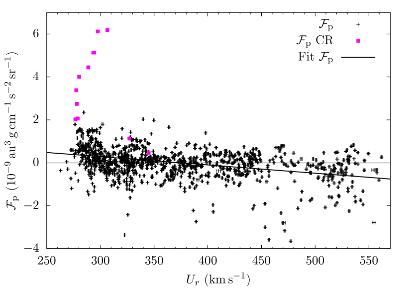
Figure 4: Dependence of the proton contribution $\mathcal{F}_{\mathrm{p}}$ to the angular-momentum flux on the radial proton bulk speed $U_{r}$. We show the measurements of $\mathcal{F}_{\mathrm{p}}$ as points and overplot the linear fit to Eq. (5) as a black line. All measurement points have horizontal and vertical error bars, which are small due to the time-averaging. The fit parameters are given in Table 2. The magenta squares represent the measurements of $\mathcal{F}_{\mathrm{p}}$ during the time of the compression region (CR) on 2020-09-06.

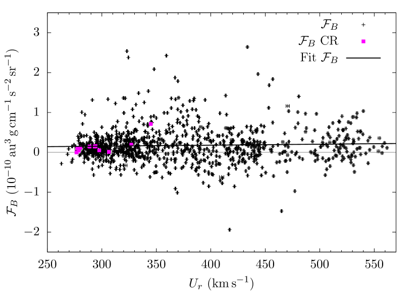
Figure 5: Dependence of the magnetic-field contribution $\mathcal{F}_{B}$ to the angular-momentum flux on the radial proton bulk speed $U_{r}$. We show the measurements of $\mathcal{F}_{B}$ as points and overplot the linear fit to Eq. (5) as a black line. All measurement points have horizontal and vertical error bars, which are small due to the time-averaging. The fit parameters are given in Table 2. The magenta squares represent the measurements of $\mathcal{F}_{B}$ during the time of the compression region (CR) on 2020-09-06.

Figure 4 shows our measurements of $\mathcal{F}_{\mathrm{p}}$ as a function of $U_{r}$. This visualisation confirms the significant $U_{r}$-dependence of the angular-momentum flux, which has been noted in previous studies and is discussed further in Section 4. The particle contribution to the angular-momentum flux shows a stronger relative variation in slow wind compared to fast wind. We also observe a trend towards negative values of $\mathcal{F}_{\mathrm{p}}$ (and thus $\mathcal{F}_{\mathrm{tot}}$) at larger $U_{r}$. Figure 5 shows the same but for $\mathcal{F}_{B}$. The magnetic-field contribution does not follow the same clear trend in its $U_{r}$-dependence as $\mathcal{F}_{\mathrm{p}}$. Figures 4 and 5 include horizontal and vertical error bars to represent $\Delta U_{r}$, $\Delta\mathcal{F}_{\mathrm{p}}$, and $\Delta\mathcal{F}_{B}$. The error bars follow from error propagation of the individual measurement uncertainties quoted in Section 2, which corresponds to the application of the standard error of the mean based on the individual uncertainties. We find that, in our hourly averages, the relative errors $\Delta U_{r}$, $\Delta\mathcal{F}_{\mathrm{p}}$, and $\Delta\mathcal{F}_{B}$ are negligible.

A comparison of the magenta points in Figures 4 and 5 reveals that $\mathcal{F}_{B}$ is not enhanced in the compression region compared to the time intervals outside the compression region. We note that the unit on the vertical axis in Figure 5 is one order of magnitude smaller than the unit on the vertical axis in Figure 4. This reflects again that $\mathcal{F}_{\mathrm{p}}$ is on average the dominant contribution to $\mathcal{F}_{\mathrm{tot}}$. In order to quantify the $U_{r}$-dependence, we apply least-squares Marquardt–Levenberg fits to our measurements according to the linear equation

$$\mathcal{F}=aU_{r}+b$$ (5)

with the fit parameters $a$ and $b$, where $\mathcal{F}$ represents either $\mathcal{F}_{\mathrm{p}}$, $\mathcal{F}_{B}$, or $\mathcal{F}_{\mathrm{tot}}$. We show the resulting fit parameters including their errors in Table 2.

Table 2: Results of our linear fits to the $U_{r}$-dependence of $\mathcal{F}_{\mathrm{p}}$, $\mathcal{F}_{B}$, and $\mathcal{F}_{\mathrm{tot}}$ according to Eq. (5).

	$a$	$b$
	$(10^{-17}\,\mathrm{au}^{3}\,\mathrm{g}\,\mathrm{cm}^{-2}\,\mathrm{s}^{-1}\,\mathrm{sr}^{-1})$	$(10^{-9}\,\mathrm{au}^{3}\,\mathrm{g}\,\mathrm{cm}^{-1}\,\mathrm{s}^{-2}\,\mathrm{sr}^{-1})$
$\mathcal{F}_{\mathrm{p}}$	$-3.86\pm 0.32$	$1.45\pm 0.12$
$\mathcal{F}_{B}$	$0.024\pm 0.017$	$0.0082\pm 0.0065$
$\mathcal{F}_{\mathrm{tot}}$	$-3.84\pm 0.32$	$1.45\pm 0.12$

3.4 Mass-flux dependence of the angular-momentum flux

We define the proton mass flux per solid-angle element as

$$\mathcal{G}_{\mathrm{p}}=r^{2}\rho U_{r}.$$ (6)

As $\mathcal{F}_{\mathrm{p}}$ is carried by the proton flow, we combine $\mathcal{F}_{\mathrm{p}}$ and $\mathcal{G}_{\mathrm{p}}$ in Figure 6 and analyse their dependence. We colour-code each measurement point with its associated value of $U_{r}$, which allows us to link Figure 6 with Figure 4. All time intervals with $\mathcal{G}_{\mathrm{p}}\gtrsim 2\times 10^{-15}\,\mathrm{au}^{2}\,\mathrm{g\,cm}^{-2}\,\mathrm{s}^{-1}\,\mathrm{sr}^{-1}$ in our dataset exhibit $\mathcal{F}_{\mathrm{p}}>0$. The majority of these points correspond to the compression region on 2020-09-06. We highlight them as magenta squares in Figure 6, illustrating that the mass-flux dependence is a useful method to separate transient and atypical plasma intervals from the regular background solar wind (see also Stansby et al., 2019).

The value of $rU_{\phi}$ is a measure of the local specific angular momentum per proton. Since $\mathcal{F}_{\mathrm{p}}=rU_{\phi}\mathcal{G}_{\mathrm{p}}$, isocontours of constant $rU_{\phi}$ correspond to bent curves when using a logarithmic $\mathcal{G}_{\mathrm{p}}$-axis in Figure 6. We show these isocontours as grey dashed curves for a range of $rU_{\phi}$ values from $\pm 10$ to $\pm 40\,\mathrm{au\,km\,s}^{-1}$. At the low-$\mathcal{G}_{\mathrm{p}}$ end, the distribution scatters almost symmetrically around a value of $\mathcal{F}_{\mathrm{p}}=0$. The envelope of the distribution in this $\mathcal{G}_{\mathrm{p}}$ range follows isocontours of constant $\pm\left|rU_{\phi}\right|$, meaning that the scatter in $\mathcal{F}_{\mathrm{p}}$ is well defined by a fixed range of constant magnitudes of the angular momentum per proton. At intermediate $\mathcal{G}_{\mathrm{p}}$, the symmetry around $\mathcal{F}_{\mathrm{p}}=0$ breaks, and more data points occur at $\mathcal{F}_{\mathrm{p}}>0$. At $\mathcal{F}_{\mathrm{p}}>0$, the envelope of the data distribution in terms of $rU_{\phi}$ decreases as $\mathcal{G}_{\mathrm{p}}$ increases in the intermediate-$\mathcal{G}_{\mathrm{p}}$ range. The points representing the compression region largely lie on the same isocontours of $rU_{\phi}$ as the bulk of the slow solar wind. This behaviour suggests that the increase in $\mathcal{F}_{\mathrm{p}}$ associated with the compression region is mostly due to an increase in $\rho$ rather than to an increase in the specific angular momentum per proton compared to the regular slow wind.

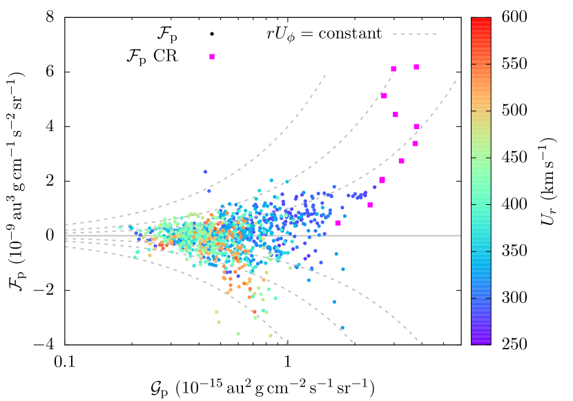
Figure 6: Dependence of the proton contribution $\mathcal{F}_{\mathrm{p}}$ to the angular-momentum flux on the radial proton mass flux $\mathcal{G}_{\mathrm{p}}$. The point colour represents the value of $U_{r}$ for each measurement. The magenta squares represent the measurements of $\mathcal{F}_{\mathrm{p}}$ during the time of the compression region (CR) on 2020-09-06. The grey dashed lines indicate contours of constant $rU_{\phi}$.

3.5 Spectral analysis of angular-momentum flux

Solar Orbiter’s high time resolution in the measurement of both the particles and the magnetic field enables the analysis of the power spectrum of the variable angular-momentum flux over a wide range of frequencies. In order to demonstrate the suitability of Solar Orbiter data for future studies of this type, we present such a spectral analysis of the angular-momentum flux based on our dataset. We apply a non-uniform fast Fourier transform (Barnett et al., 2019; Barnett, 2021) to the timeseries data of $\mathcal{F}_{\mathrm{p}}$ and $\mathcal{F}_{B}$ throughout our entire dataset. For this calculation, we use 1-minute averages of the data instead of the 60-minute averages used in our study otherwise. This choice allows us to explore the variability of $\mathcal{F}_{\mathrm{p}}$ and $\mathcal{F}_{B}$ over a wider range of frequencies. Figure 7 shows the resulting power spectral densities (PSDs) of $\mathcal{F}_{\mathrm{p}}$ and $\mathcal{F}_{B}$ as functions of frequency $\nu$.

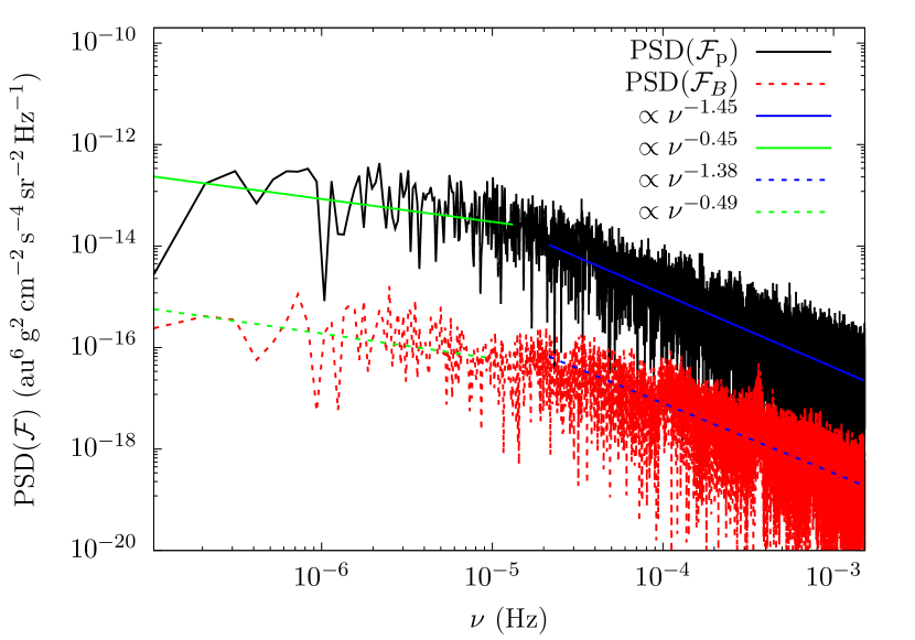
Figure 7: Power spectral densities (PSDs) of $\mathcal{F}_{\mathrm{p}}$ and $\mathcal{F}_{B}$. The straight lines show power-law fits of the partial spectra of $\mathcal{F}_{\mathrm{p}}$ and $\mathcal{F}_{B}$.

We observe a spectral break in the PSDs of both contributions to the angular-momentum flux near a frequency of $\nu\approx 10^{-5}\,\mathrm{Hz}$. We perform separate power-law fits to PSD($\mathcal{F}_{\mathrm{p}}$) and PSD($\mathcal{F}_{B}$) on both sides of their spectral breakpoints. We find PSD($\mathcal{F}_{\mathrm{p}}$)$\propto\nu^{-0.45\pm 0.12}$ in the low-$\nu$ regime and PSD($\mathcal{F}_{\mathrm{p}}$)$\propto\nu^{-1.448\pm 0.012}$ in the high-$\nu$ regime. Likewise, PSD($\mathcal{F}_{B}$)$\propto\nu^{-0.49\pm 0.14}$ in the low-$\nu$ regime and PSD($\mathcal{F}_{B}$)$\propto\nu^{-1.377\pm 0.012}$ in the high-$\nu$ regime. We overplot the fit results in Figure 7.

4 Discussion

Our measurements of $|\mathcal{F}_{\mathrm{p}}|$ are largely in agreement with previous measurements in the solar wind, which reveal values of about $4.4\dots 5.9\times 10^{-11}\,\mathrm{au}^{3}\,\mathrm{g\,cm}^{-1}\,\mathrm{s}^{-2}\,\mathrm{sr}^{-1}$ (Pizzo et al., 1983), $4.4\dots 11.2\times 10^{-11}\,\mathrm{au}^{3}\,\mathrm{g\,cm}^{-1}\,\mathrm{s}^{-2}\,\mathrm{sr}^{-1}$ (Finley et al., 2020), and $1.09\dots 2.43\times 10^{-10}\,\mathrm{au}^{3}\,\mathrm{g\,cm}^{-1}\,\mathrm{s}^{-2}\,\mathrm{sr}^{-1}$ (Liu et al., 2021) as averages over their whole datasets.

As shown in Section 3.3, we find a general trend of decreasing $\mathcal{F}_{\mathrm{p}}$ with increasing $U_{r}$, consistent with previous findings in data from Wind and Parker Solar Probe (Finley et al., 2019, 2020, 2021) and with estimates based on the observation of the Earth’s magnetotail deflection (Němeček et al., 2020). The observation of this trend in near-Sun data suggests that the trend is generated close to the Sun and not by local deflections at large distances. On average, $\mathcal{F}_{\mathrm{p}}>0$ for $U_{r}\lesssim 376\,\mathrm{km\,s}^{-1}$ and $\mathcal{F}_{\mathrm{p}}<0$ for $U_{r}\gtrsim 376\,\mathrm{km\,s}^{-1}$ according to our fit result applied to the data shown in Figure 4. The magnetic-field contribution $\mathcal{F}_{B}$ shows only a small dependence on $U_{r}$, which is consistent with recent measurements from Parker Solar Probe (Liu et al., 2021).

Averaged over very long timescales, we expect both the particle contribution and the magnetic-field contribution to the angular-momentum flux to be positive due to the Sun’s sense of rotation and the direction of the average Parker (1958) field. In addition, we anticipate an overall loss of the Sun’s angular momentum based on observed trends in the rotation periods of Sun-like stars, which decrease with age along the main sequence. This finding is generally interpreted as a consequence of magnetised stellar winds (Lorenzo-Oliveira et al., 2019; do Nascimento et al., 2020). In the Sun’s specific case, a positive net $\mathcal{F}_{\mathrm{tot}}$ corresponds to a net loss of the Sun’s rotational angular momentum.

Moreover, we expect the average relative contribution of $\mathcal{F}_{B}$ to the total angular-momentum flux to decrease slightly with increasing heliocentric distance as magnetic stress is converted into particle angular momentum (Weber & Davis, 1967), although Marsch & Richter (1984) do not find clear evidence for this behaviour within 1 au. Previous measurements of $\mathcal{F}_{B}$ reveal values of about $4.1\dots 4.7\times 10^{-11}\,\mathrm{au}^{3}\,\mathrm{g\,cm}^{-1}\,\mathrm{s}^{-2}\,\mathrm{sr}^{-1}$ (Pizzo et al., 1983), $3.6\dots 4.7\times 10^{-11}\,\mathrm{au}^{3}\,\mathrm{g\,cm}^{-1}\,\mathrm{s}^{-2}\,\mathrm{sr}^{-1}$ (Finley et al., 2020), and $2.1\dots 3.8\times 10^{-11}\,\mathrm{au}^{3}\,\mathrm{g\,cm}^{-1}\,\mathrm{s}^{-2}\,\mathrm{sr}^{-1}$ (Liu et al., 2021) as averages over their whole datasets at small heliocentric distances. These values are indeed greater than our mean values measured at Solar Orbiter’s distances from the Sun, consistent with an average transfer of angular momentum from the field to the particles taking place between 0.3 and 0.7 au. Averaged over two solar cycles, Finley et al. (2019) find $\mathcal{F}_{B}\approx 3.58\times 10^{-11}\,\mathrm{au}^{3}\,\mathrm{g\,cm}^{-1}\,\mathrm{s}^{-2}\,\mathrm{sr}^{-1}$ in data from the Wind spacecraft at 1 au. Comparing to the averages at small heliocentric distances, this 1-au long-term average is also consistent with an overall decreasing trend of $\mathcal{F}_{B}$ with increasing $r$. We note, however, that our average $\mathcal{F}_{B}$ at intermediate distances is even smaller than the 1-au long-term average from Wind. This discrepancy is probably the result of the limited statistics in our dataset and the specific solar wind streams encountered by Solar Orbiter during its first orbit at this particular phase of the solar cycle. Radial alignments between Solar Orbiter, Parker Solar Probe, and potentially other assets with suitable pointing accuracy and instrumentation will help us to understand the partition of the contributions to the angular-momentum flux over longer time intervals in the future. In general, we expect a significant dependence of the angular-momentum flux on the Sun’s 11-year activity cycle based on changes to the global magnetic field strength and changing solar-wind source regions (Finley et al., 2018).

Notwithstanding these expectations regarding large-scale behaviour, our measurements reveal the large variation of the angular-momentum flux over many timescales from a few hours to months. Taking our full measurement time interval into account, the relative variations in $\mathcal{F}_{\mathrm{p}}$ are greater than the relative variations in $\mathcal{F}_{B}$. When separating fast and slow wind, however, the relative variations in $\mathcal{F}_{B}$ are greater than those in $\mathcal{F}_{\mathrm{p}}$ both in the intervals with slow ($U_{r}<400\,\mathrm{km\,s}^{-1}$) and in the intervals with fast ($U_{r}>500\,\mathrm{km\,s}^{-1}$) solar wind. A potential reason for this behaviour lies in the fact that $\mathcal{F}_{B}$ does not directly depend on $U_{r}$, while $\mathcal{F}_{\mathrm{p}}$ changes significantly with $U_{r}$ (see Figures 4 and 5). We attribute the natural variations in the angular-momentum flux to changes in the solar-wind source regions (Schwenn, 2006; Tindale & Chapman, 2017), deflections during the expansion (Egidi et al., 1969; Siscoe et al., 1969), or large-scale fluctuations as part of the turbulent spectrum (Tu & Marsch, 1995; Bruno & Carbone, 2013). Furthermore, the complex field and flow geometries in the low corona and latitudinal variations of the source regions create variations in $\mathcal{F}_{\mathrm{tot}}$ (Finley & Matt, 2017; Réville & Brun, 2017; Boe et al., 2020; Finley et al., 2020).

Figure 6 confirms that the scatter of data points around $\mathcal{F}_{\mathrm{p}}=0$ is more symmetric in the tenuous, low-$\mathcal{G}_{\mathrm{p}}$ wind than in the denser, high-$\mathcal{G}_{\mathrm{p}}$ wind. Assuming that all wind is ejected from the Sun with positive $\mathcal{F}_{\mathrm{p}}$ due to the Sun’s sense of rotation, negative $\mathcal{F}_{\mathrm{p}}$ can only be created by local stream interactions, which in turn must increase $\mathcal{F}_{\mathrm{p}}$ of neighbouring plasma in order to fulfil angular-momentum conservation. Our observation of a more symmetric distribution around $\mathcal{F}_{\mathrm{p}}=0$ at low $\mathcal{G}_{\mathrm{p}}$ is then consistent with a scenario in which these local stream interactions occur more effectively in low-$\mathcal{G}_{\mathrm{p}}$ wind. In this scenario, the mixing of $\mathcal{F}_{\mathrm{p}}$ in low-$\mathcal{G}_{\mathrm{p}}$ wind leaves the high-$\mathcal{G}_{\mathrm{p}}$ wind as the main carrier of net angular-momentum flux. Figure 6 then suggests that most of the net angular-momentum flux in the solar wind is carried by dense slow wind with $\mathcal{F}_{\mathrm{p}}>0$ in the intermediate-to-high-$\mathcal{G}_{\mathrm{p}}$ range.

Our spectral analysis of $\mathcal{F}_{\mathrm{p}}$ and $\mathcal{F}_{B}$ in Section 3.5 quantifies the variations of the angular-momentum flux depending on frequency $\nu$. The averaging time (60 minutes) for our analysis of the angular-momentum flux outside of Section 3.5 corresponds to $\nu=2.78\times 10^{-4}\,\mathrm{Hz}$, which lies well inside the accessible frequency range of the high-$\nu$ regime. Figure 7 does not exhibit a clear peak at the frequency associated with the Sun’s equatorial rotation frequency, $\nu=2\pi\Omega_{\odot}\approx 4.7\times 10^{-7}\,\mathrm{Hz}$. The lack of such a feature suggests that the variability of the angular-momentum flux induced by repeated passes of source regions due to the Sun’s rotation is negligible in our dataset. However, a spectral analysis of variations on these long timescales is not fully reliable at this stage of the mission due to the short overall duration of the dataset and its patchiness. The smallest gaps in our dataset are of order a few minutes, while the longest gap is 18 days long. We note in this context that large-scale interplanetary structures such as co-rotating interaction regions, which could be responsible for variations on these timescales, typically decay after a few revolutions. The breakpoint at $\nu\sim 10^{-5}\,\mathrm{Hz}$ corresponds to a timescale of $\sim 28\,\mathrm{h}$. Assuming that this variation is frozen into the solar-wind flow, this timescale corresponds to a convected length scale of $\sim 0.27\,\mathrm{au}$ according to Taylor’s hypothesis (Taylor, 1938) based on an average $U_{r}\approx 400\,\mathrm{km\,s}^{-1}$. This scale is greater than the typical correlation length in solar-wind turbulence in the inner heliosphere (Matthaeus & Goldstein, 1982; Bruno & Dobrowolny, 1986; Bruno & Carbone, 2013; Bourouaine et al., 2020). We note, however, that the uncertainty in the visual determination of the breakpoint frequency permits values between $\sim 6\times 10^{-6}\,\mathrm{Hz}$ and $\sim 4\times 10^{-5}\,\mathrm{Hz}$ due to the noise in our Fourier spectrum. Length scales within the corresponding range of breakpoint scales are still greater than the typical correlation length. In addition, the determination of the correlation length itself is to a certain degree method-dependent. Some estimates for the correlation length of velocity fluctuations provide the same order of magnitude as the length scale associated with our breakpoint in $\mathrm{PSD}(\mathcal{F}_{\mathrm{p}})$ (Podesta et al., 2008), supporting the link between fluctuations in angular-momentum flux with the turbulent fluctuations in the solar wind. It is worthwhile to perform a scale-dependent study of the angular-momentum flux in the future, especially by separating the variations in the low-$\nu$ regime and in the high-$\nu$ regime.

Sporadic events, such as the compression on 2020-09-06, contribute to the natural variations of the angular-momentum flux. We do not remove events like these from our statistical analysis, although they introduce a bias as seen in Figures 1 and 2. The on-average greater variations in slow solar wind are reflected by the greater variation of the proton contribution $\mathcal{F}_{\mathrm{p}}$ to the angular-momentum flux at small $U_{r}$ in Figure 4. The mass-flux dependence of $\mathcal{F}_{\mathrm{p}}$ during the time interval associated with the compression region in Figure 6 reveals a way to separate dense intermittent structures for future analyses. Using this method, it will be interesting to investigate the contribution of co-rotating interaction regions, coronal mass ejections, and other transient mass-flux enhancements to the Sun’s long-term angular-momentum loss. In fact, the amount of angular momentum carried by coronal mass ejections is still not well known. Since angular momentum is conserved, however, local angular-momentum enhancements by the deflection of background solar wind must be balanced via flows with opposite angular momentum elsewhere in space. Figure 6 shows that the compression region in our dataset carries approximately the same specific angular momentum per proton, $rU_{\phi}$, as the regular slow wind, yet with a higher density. This observation suggests that the compression region represents “scooped-up” solar-wind mass, which has not undergone a significant alteration in terms of the particle’s angular momentum. As shown in Figure 5, the value of $\mathcal{F}_{B}$ in the compression region is comparable to the average value of $\mathcal{F}_{B}$ across our dataset. This observation supports our interpretation of the compression region as a density increase of otherwise unaltered background solar wind. Composition measurements of solar-wind transients have the potential to confirm this interpretation in the future.

Our measurements neglect the contribution of $\alpha$-particles to the angular-momentum flux. Given that their contribution to the local momentum flux is of order 20% (even greater near the Sun), $\alpha$-particles can make a significant contribution to the total angular-momentum flux (Pizzo et al., 1983; Marsch & Richter, 1984; Verscharen et al., 2015; Finley et al., 2021). Both Finley et al. (2021) and Liu et al. (2021) suggest a reconstruction of the $\alpha$-particle component based on the field-alignment of the differential flow between protons and $\alpha$-particles. It is still an open question, however, whether the $\alpha$-particles are in general a net source of positive or negative angular-momentum flux. In addition, the proton beam component can carry a significant angular momentum flux (Finley et al., 2021), which we directly subsume through our using of total proton moments for $\rho$ and $\@vec{U}$. Our analysis also neglects stresses due to pressure anisotropies in the particle populations (Hundhausen, 1970; Marsch et al., 1982; Verscharen et al., 2019). This contribution to the angular-momentum flux is not significant for most of the solar-wind plasma though.

At this early stage of the mission, it is difficult to quantify the measurement uncertainties of the instruments accurately. These estimates will become more reliable as the mission progresses. At $U_{r}\lesssim 300\,\mathrm{km\,s}^{-1}$, the sensitivity of SWA/PAS decreases, so that the uncertainty in the proton moments increases. Therefore, we urge caution regarding the interpretation of the proton data (especially, the proton density) in this velocity range, which includes the compression region. Solar Orbiter’s Radio and Plasma Waves (RPW, Maksimovic et al., 2020) instrument provides an estimate of the local electron density based on the probe-to-spacecraft potential and quasi-thermal noise measurements (Khotyaintsev et al., 2021) which is independent of the SWA/PAS density measurement. We find that, especially during intervals with low $U_{r}$, SWA/PAS provides a greater density value than RPW. In Appendix A, we repeat part of our analysis using the independent RPW density estimate. Although we find a reduction in the peaks of $\mathcal{F}_{\mathrm{p}}$ when using the RPW density, our conclusions hold regardless of the used density measurement. RPW is also able to provide an independent measurement of $|\@vec{U}|$ from the bias DC electric field combined with the measurement of $|\@vec{B}|$ from MAG. A careful cross-calibration between SWA/PAS and RPW both in terms of density and bulk-speed measurements will improve further studies in the future (Owen et al., 2020; Maksimovic et al., 2020; Walsh et al., 2020).

Early results from Parker Solar Probe report an increased azimuthal flow of the protons compared to the expectation of the Weber & Davis (1967) model at heliocentric distances up to about 0.23 au (Kasper et al., 2019). Possible explanations for this observed “angular-momentum paradox” (Réville et al., 2020) include the partitioning of angular-momentum flux between the different particle species, non-axisymmetric flows and pressure gradients, and pressure anisotropies. In our data, however, we do not find evidence for such a persistent positive azimuthal flow, albeit our data were recorded at distances greater than 0.59 au and show a different distribution of solar-wind speeds compared to the study by Kasper et al. (2019). In the future, when Solar Orbiter’s perihelion distance is reduced, it will be important to monitor the azimuthal flow of the protons more closely to compare with Parker Solar Probe’s findings of super-rotational flows in the near-Sun solar wind.

5 Concluding remarks

A reliable quantification of the Sun’s global angular-momentum loss requires measurements of the angular-momentum flux over long time intervals. In addition, we require distinctive measurements of typical equatorial and polar solar wind (McComas et al., 2000; Verscharen et al., 2021) to complete the understanding of the global angular-momentum loss. At this early point in the mission, we cannot confidently ascertain our measurement interval as a representative sample of the solar wind’s angular-momentum flux. Further long-term studies will become available during Solar Orbiter’s mission lifetime. In later stages of the mission, the spacecraft will leave the plane of the ecliptic making observations of the angular-momentum flux of polar solar wind feasible. Nevertheless, our study already confirms the potential for future detailed studies of the large-scale properties of the solar wind with the data from Solar Orbiter.

Appendix A The angular-momentum and mass flux based on the RPW density

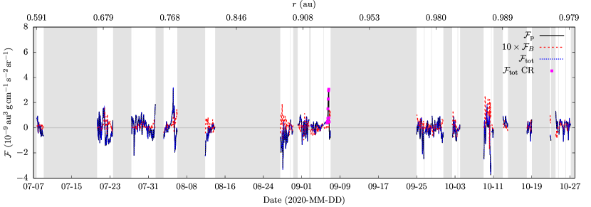
Figure 8: Same as Figure 1, but using $\rho$ from RPW in the calculation of $\mathcal{F}_{\mathrm{p}}$ and $\mathcal{F}_{\mathrm{tot}}$. The grey-shaded areas indicate times for which our merged SWA/PAS-MAG-RPW data product is unavailable or the data flags for either dataset indicate poor data quality.

RPW measures the local total electron density $n_{\mathrm{e}}$ based on a combination of both the peak-tracking of the plasma frequency and the spacecraft potential (Khotyaintsev et al., 2021). Due to quasi-neutrality, $n_{\mathrm{e}}$ serves as an independent measure of the total charge-weighted ion density. For comparison with our SWA/PAS-MAG measurements, we create a new dataset using $\@vec{U}$ from SWA/PAS, $\@vec{B}$ from MAG, and $\rho=m_{\mathrm{p}}n_{\mathrm{e}}$ from RPW, where $m_{\mathrm{p}}$ is the proton mass. We apply the same selection, averaging, and analysis methods as in the main part of this work. This leaves us with 913 data points for our combined SWA/PAS-MAG-RPW dataset in total.

We show the timeseries of our combined SWA/PAS-MAG-RPW dataset in Figure 8. Qualitatively, the timeseries agrees with Figure 1. However, the peaks with $\mathcal{F}_{\mathrm{p}}>0$ are less pronounced in the SWA/PAS-MAG-RPW dataset than in the SWA/PAS-MAG dataset. These peaks, including our compression region on 2020-09-06, correspond to intervals of slow and dense solar wind, for which the SWA/PAS and RPW densities diverge most.

We present the statistical properties of our combined SWA/PAS-MAG-RPW dataset in Table 3. Due to the lower peaks in $\mathcal{F}_{\mathrm{p}}$, the signs of the mean values for $\mathcal{F}_{\mathrm{p}}$ and $\mathcal{F}_{\mathrm{tot}}$ across our full dataset are now different from the signs of the SWA/PAS-MAG dataset shown in Table 1. The maxima of $\mathcal{F}_{\mathrm{p}}$ and $\mathcal{F}_{\mathrm{tot}}$ in Table 3 are lower than those given in Table 1, reflecting the lower peaks seen in Figure 8. All other statistical markers in Table 3 agree with our results shown in Table 1.

Table 3: Same as Table 1, but using $\rho$ from RPW in the calculation of $\mathcal{F}_{\mathrm{p}}$ and $\mathcal{F}_{\mathrm{tot}}$.

	mean	min	max
	$(10^{-11}\,\mathrm{au}^{3}\,\mathrm{g}\,\mathrm{cm}^{-1}\,\mathrm{s}^{-2}\,\mathrm{sr}^{-1})$	$(10^{-9}\,\mathrm{au}^{3}\,\mathrm{g}\,\mathrm{cm}^{-1}\,\mathrm{s}^{-2}\,\mathrm{sr}^{-1})$	$(10^{-9}\,\mathrm{au}^{3}\,\mathrm{g}\,\mathrm{cm}^{-1}\,\mathrm{s}^{-2}\,\mathrm{sr}^{-1})$
all speeds
$\mathcal{F}_{\mathrm{p}}$	$-5.33\pm 72.20$	$-3.76$	$3.12$
$\mathcal{F}_{B}$	$1.67\pm 4.24$	$-0.169$	$0.254$
$\mathcal{F}_{\mathrm{tot}}$	$-3.66\pm 72.20$	$-3.69$	$3.21$
$U_{r}<400\,\mathrm{km\,s}^{-1}$
$\mathcal{F}_{\mathrm{p}}$	$10.5\pm 70.5$	$-2.49$	$3.12$
$\mathcal{F}_{B}$	$0.735\pm 5.840$	$-0.230$	$0.254$
$\mathcal{F}_{\mathrm{tot}}$	$11.2\pm 70.3$	$-2.49$	$3.21$
$U_{r}>500\,\mathrm{km\,s}^{-1}$
$\mathcal{F}_{\mathrm{p}}$	$-67.2\pm 106.5$	$-5.43$	$0.753$
$\mathcal{F}_{B}$	$0.605\pm 5.464$	$-0.174$	$0.101$
$\mathcal{F}_{\mathrm{tot}}$	$-66.6\pm 108.6$	$-5.57$	$0.836$

We show the dependence of $\mathcal{F}_{\mathrm{p}}$ on $\mathcal{G}_{\mathrm{p}}$ for our combined SWA/PAS-MAG-RPW dataset in Figure 9. The comparison between Figures 6 and 9 shows that most high-$\mathcal{G}_{\mathrm{p}}$ measurements, including the compression region, shift towards smaller values of $\mathcal{G}_{\mathrm{p}}$ when using the RPW density estimate. In addition, the compression region shifts towards smaller values of $\mathcal{F}_{\mathrm{p}}$. Notwithstanding these differences, our conclusions drawn based on Figure 6 are still valid.

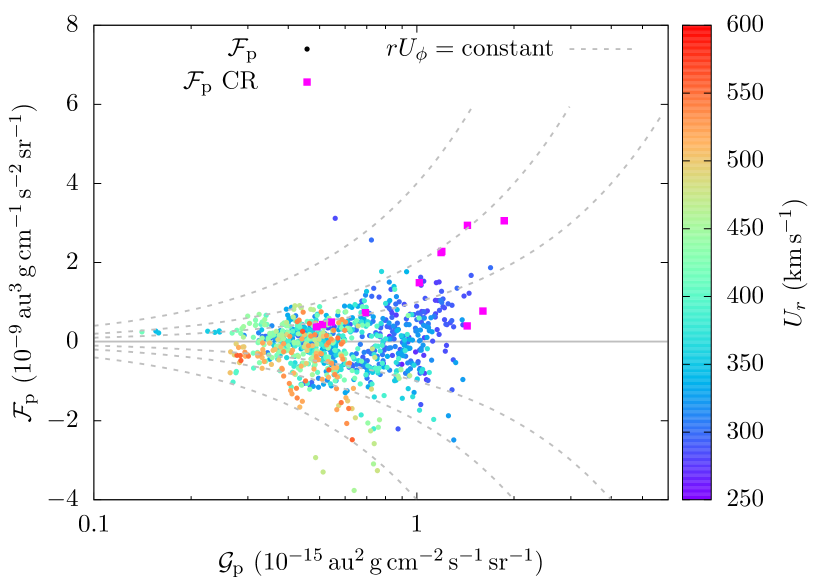
Figure 9: Same as Figure 6, but using $\rho$ from RPW in the calculation of $\mathcal{F}_{\mathrm{p}}$ and $\mathcal{G}_{\mathrm{p}}$.

References

- Allen et al. (2020) Allen, R. C., Lario, D., Odstrcil, D., et al. 2020, ApJS, 246, 36
- Barnes (2003) Barnes, S. A. 2003, ApJ, 586, 464
- Barnett (2021) Barnett, A. H. 2021, Appl. Comput. Harmon. Anal., 51, 1
- Barnett et al. (2019) Barnett, A. H., Magland, J. F., & Klinteberg, L. a. 2019, SIAM J. Sci. Comp., 41, C479
- Boe et al. (2020) Boe, B., Habbal, S., & Druckmüller, M. 2020, ApJ, 895, 123
- Bourouaine et al. (2020) Bourouaine, S., Perez, J. C., Klein, K. G., et al. 2020, ApJ, 904, L30
- Bruno & Carbone (2013) Bruno, R. & Carbone, V. 2013, Living Reviews in Solar Physics, 10, 2
- Bruno & Dobrowolny (1986) Bruno, R. & Dobrowolny, M. 1986, Annales Geophysicae, 4, 17
- do Nascimento et al. (2020) do Nascimento, J. D., J., de Almeida, L., Velloso, E. N., et al. 2020, ApJ, 898, 173
- Egidi et al. (1969) Egidi, A., Pizzella, G., & Signorini, C. 1969, J. Geophys. Res., 74, 2807
- Finley et al. (2019) Finley, A. J., Hewitt, A. L., Matt, S. P., et al. 2019, ApJ, 885, L30
- Finley & Matt (2017) Finley, A. J. & Matt, S. P. 2017, ApJ, 845, 46
- Finley et al. (2020) Finley, A. J., Matt, S. P., Réville, V., et al. 2020, ApJ, 902, L4
- Finley et al. (2018) Finley, A. J., Matt, S. P., & See, V. 2018, ApJ, 864, 125
- Finley et al. (2021) Finley, A. J., McManus, M. D., Matt, S. P., et al. 2021, A&A, 650, A17
- Fox et al. (2016) Fox, N. J., Velli, M. C., Bale, S. D., et al. 2016, Space Sci. Rev., 204, 7
- Gallet & Bouvier (2013) Gallet, F. & Bouvier, J. 2013, A&A, 556, A36
- García Marirrodriga et al. (2021) García Marirrodriga, C., Pacros, A., Strandmoe, S., et al. 2021, A&A, accepted
- Horbury et al. (2020) Horbury, T. S., O’Brien, H., Carrasco Blazquez, I., et al. 2020, A&A, 642, A9
- Hundhausen (1970) Hundhausen, A. J. 1970, Reviews of Geophysics and Space Physics, 8, 729
- Hundhausen et al. (1970) Hundhausen, A. J., Bame, S. J., Asbridge, J. R., & Sydoriak, S. J. 1970, J. Geophys. Res., 75, 4643
- Kasper et al. (2019) Kasper, J. C., Bale, S. D., Belcher, J. W., et al. 2019, Nature, 576, 228
- Khotyaintsev et al. (2021) Khotyaintsev, Y. V., Graham, D. B., Vaivads, A., Steinvall, L., & et al. 2021, A&A, this issue
- Lazarus & Goldstein (1971) Lazarus, A. J. & Goldstein, B. E. 1971, ApJ, 168, 571
- Liu et al. (2021) Liu, Y. D., Chen, C., Stevens, M. L., & Liu, M. 2021, ApJ, 908, L41
- Lorenzo-Oliveira et al. (2019) Lorenzo-Oliveira, D., Meléndez, J., Yana Galarza, J., et al. 2019, MNRAS, 485, L68
- Maksimovic et al. (2020) Maksimovic, M., Bale, S. D., Chust, T., et al. 2020, A&A, 642, A12
- Marsch & Richter (1984) Marsch, E. & Richter, A. K. 1984, J. Geophys. Res., 89, 5386
- Marsch et al. (1982) Marsch, E., Schwenn, R., Rosenbauer, H., et al. 1982, J. Geophys. Res., 87, 52
- Matt et al. (2015) Matt, S. P., Brun, A. S., Baraffe, I., Bouvier, J., & Chabrier, G. 2015, ApJ, 799, L23
- Matthaeus & Goldstein (1982) Matthaeus, W. H. & Goldstein, M. L. 1982, J. Geophys. Res., 87, 6011
- McComas et al. (2000) McComas, D. J., Barraclough, B. L., Funsten, H. O., et al. 2000, J. Geophys. Res., 105, 10419
- Mestel (1968) Mestel, L. 1968, MNRAS, 138, 359
- Möstl et al. (2020) Möstl, C., Weiss, A. J., Bailey, R. L., et al. 2020, ApJ, 903, 92
- Müller et al. (2020) Müller, D., St. Cyr, O. C., Zouganelis, I., et al. 2020, A&A, 642, A1
- Neugebauer & Snyder (1962) Neugebauer, M. & Snyder, C. W. 1962, Science, 138, 1095
- Němeček et al. (2020) Němeček, Z., Ďurovcová, T., Šafránková, J., et al. 2020, ApJ, 897, L39
- Owen et al. (2020) Owen, C. J., Bruno, R., Livi, S., et al. 2020, A&A, 642, A16
- Pantolmos & Matt (2017) Pantolmos, G. & Matt, S. P. 2017, ApJ, 849, 83
- Parker (1958) Parker, E. N. 1958, ApJ, 128, 664
- Pizzo et al. (1983) Pizzo, V., Schwenn, R., Marsch, E., et al. 1983, ApJ, 271, 335
- Podesta et al. (2008) Podesta, J. J., Galvin, A. B., & Farrugia, C. J. 2008, Journal of Geophysical Research (Space Physics), 113, A09104
- Reiners & Mohanty (2012) Reiners, A. & Mohanty, S. 2012, ApJ, 746, 43
- Réville & Brun (2017) Réville, V. & Brun, A. S. 2017, ApJ, 850, 45
- Réville et al. (2020) Réville, V., Velli, M., Panasenco, O., et al. 2020, ApJS, 246, 24
- Richter & Luttrell (1986) Richter, A. K. & Luttrell, A. H. 1986, J. Geophys. Res., 91, 5873
- Schwenn (2006) Schwenn, R. 2006, Space Sci. Rev., 124, 51
- Siscoe et al. (1969) Siscoe, G. L., Goldstein, B., & Lazarus, A. J. 1969, J. Geophys. Res., 74, 1759
- Stansby et al. (2019) Stansby, D., Horbury, T. S., & Matteini, L. 2019, MNRAS, 482, 1706
- Taylor (1938) Taylor, G. I. 1938, Proceedings of the Royal Society of London Series A, 164, 476
- Tindale & Chapman (2017) Tindale, E. & Chapman, S. C. 2017, Journal of Geophysical Research (Space Physics), 122, 9824
- Tu & Marsch (1995) Tu, C. Y. & Marsch, E. 1995, Space Sci. Rev., 73, 1
- Verscharen et al. (2021) Verscharen, D., Bale, S. D., & Velli, M. 2021, MNRAS, submitted
- Verscharen et al. (2015) Verscharen, D., Chandran, B. D. G., Bourouaine, S., & Hollweg, J. V. 2015, ApJ, 806, 157
- Verscharen et al. (2019) Verscharen, D., Klein, K. G., & Maruca, B. A. 2019, Living Reviews in Solar Physics, 16, 5
- Walsh et al. (2020) Walsh, A. P., Horbury, T. S., Maksimovic, M., et al. 2020, A&A, 642, A5
- Weber & Davis (1967) Weber, E. J. & Davis, Leverett, J. 1967, ApJ, 148, 217