High-redshift Narrow-line Seyfert 1 Galaxies: A Candidate Sample

Abstract

The study of narrow-line Seyfert 1 galaxies (NLS1s) is now mostly limited to low redshift ($z<0.8$) because their definition requires the presence of the H$\beta$ emission line, which is redshifted out of the spectral coverage of major ground-based spectroscopic surveys at $z>0.8$. We studied the correlation between the properties of H$\beta$ and Mg II lines of a large sample of SDSS DR14 quasars to find high-$z$ NLS1 candidates. Based on the strong correlation of $\mathrm{FWHM(MgII)=(0.880\pm 0.005)\times FWHM(H\beta)+(0.438\pm 0.018)}$, we present a sample of high-$z$ NLS1 candidates having FWHM of Mg II $<$ 2000 km s^-1. The high-$z$ sample contains 2684 NLS1s with redshift $z=0.8-2.5$ with a median logarithmic bolometric luminosity of $46.16\pm 0.42$ erg s^-1, logarithmic black hole mass of $8.01\pm 0.35M_{\odot}$, and logarithmic Eddington ratio of $0.02\pm 0.27$. The fraction of radio-detected high-$z$ NLS1s is similar to that of the low-$z$ NLS1s and SDSS DR14 quasars at a similar redshift range, and their radio luminosity is found to be strongly correlated with their black hole mass.

1 Introduction

Narrow-line Seyfert 1 galaxies (NLS1s) are a special class of active galactic nuclei (AGNs), which are characterized by narrow permitted emission lines with the full width at half maximum (FWHM) of the permitted H$\beta<2000$ km s^-1 and flux ratio [O III]/H$\beta<3$ (Osterbrock & Dahari, 1983; Goodrich, 1989). They show stronger Fe II emission, higher amplitude rapid X-ray variability, higher soft X-ray excess, and steeper soft and hard X-ray spectra compared to the broad line Seyfert 1 galaxies (BLS1s; e.g., Nandra & Pounds, 1994; Boller et al., 1996; Leighly, 1999). They are widely believed to have low black hole masses ($M_{\mathrm{BH}}$ $<$ 10⁸ M_⊙) and high accretion rates greater than 0.1 $L_{\mathrm{Edd}}$, where $L_{\mathrm{Edd}}$ is the Eddington luminosity defined as $L_{\mathrm{Edd}}=1.3\times 10^{38}\left(\frac{M_{\mathrm{BH}}}{M_{\odot}}\right)$ erg s^-1 compared to BLS1s (e.g., Grupe & Mathur, 2004; Zhou et al., 2006; Xu et al., 2012; Rakshit et al., 2017). It has been found that the optical and infrared variability of NLS1s is lower compared to BLS1s primarily due to the higher Eddington ratio in the former (see Rakshit & Stalin, 2017; Rakshit et al., 2019). The low $M_{\mathrm{BH}}$ values and high accretion rates in NLS1s indicate that they are young and growing AGN and like radio-quiet AGN may not be able to produce relativistic jets (Mathur, 2000; Grupe, 2000). The low $M_{\mathrm{BH}}$ in NLS1s could be due to the projection effects (Rakshit et al., 2017; Decarli et al., 2008). Spectropolarimetric observations (Baldi et al., 2016), as well as modeling of accretion disk spectra (Calderone et al., 2013), indicate that the $M_{\mathrm{BH}}$ values of NLS1s available in the literature are an underestimation. Recently, Viswanath et al. (2019) modeled a large sample of radio-loud NLS1s along with a control sample of radio-quiet NLS1s and BLS1s, and found that NLS1s have $M_{\mathrm{BH}}$ and Eddington ratio similar to BLS1s.

Only 7% NLS1s are detected in radio surveys (Komossa et al., 2006; Rakshit et al., 2017; Singh & Chand, 2018). This is lower than the fraction of $\sim$15% radio-loud sources found in normal AGN population (Kellermann et al., 1989). About two dozen NLS1s show extended radio emission larger than 20 kpc (see Rakshit et al., 2018b, and the references therein). A minority of radio-loud NLS1s are also detected in the GeV $\gamma$-ray band by the Fermi Gamma Ray Space Telescope unambiguously arguing for the presence of relativistic jets in them. As of today about a dozen NLS1s are known to be emitters of $\gamma$-rays (see Paliya et al., 2018, and the references therein). Broad band spectral energy distribution modeling of these $\gamma$-ray emitting NLS1s show that they have the typical two hump structure with the high energy emission due to inverse Compton scattering of seed photons external to the jets of these sources (Paliya et al., 2013, 2019). The broadband SEDs of $\gamma$-ray emitting NLSy1s are similar to the flat spectrum radio quasar (FSRQ) category of AGN. Moreover, NLS1s are predominantly hosted by disk-like galaxies (Järvelä et al., 2018; Olguín-Iglesias et al., 2020) while FSRQs are hosted in elliptical galaxies (Sikora et al., 2007). If it were to be confirmed that the host of $\gamma$-ray emitting NLS1s are indeed spirals, then we could conclude that relativistic jets are invariably launched by spiral as well as elliptical hosts.

Our current knowledge of the general physical properties of NLS1s is based on the number of sources that we know up to $z$ = 0.8 (Williams et al., 2002; Zhou et al., 2006; Rakshit & Stalin, 2017; Chen et al., 2018). Although only a couple of NLS1s are known beyond $z$ = 0.8 (Yao et al., 2015, 2019), it is possible that there are $\gamma$-ray emitting NLS1s beyond $z$ = 1. Since many of the properties of low-$z$ NLS1s are similar to FSRQs and as FSRQs are known up to large redshifts, it is natural to expect high-$z$ $\gamma$-ray emitting NLS1s. On the detection of such high-$z$ $\gamma$-ray emitting NLS1s, one can also check if the hosts of high-$z$ NLS1s are predominantly hosted by disk galaxies similar to their low-$z$ counterparts. However, detecting $\gamma$-ray emitting NLS1s beyond $z=0.8$ is hampered by the non-existent of optically known NLS1s with $z>0.8$. One approach to find more $\gamma$-ray emitting NLS1 galaxies at $z>0.8$ is first to arrive at a catalog of high-$z$ NLS1s in the optical and then look for their counterparts in the 10 years of data in Fermi. Our motivation in this work is therefore to arrive at a new catalog of high-$z$ NLS1s. However, to find NLS1 at $z>0.8$, an alternative criterion is needed wherein another strong permitted emission line could serve as a proxy for H$\beta$. Recently, Rakshit et al. (2020, hereafter R20) found that the width of the Mg II line (available along with H$\beta$ line in the SDSS spectra in the redshift range of $z=0.35-0.8$) shows a strong correlation with the line width of H$\beta$. Thus, in this paper, we investigated in detail the correlation between Mg II and H$\beta$ line properties of SDSS DR14 quasars to arrive at a sample of high-$z$ NLS1s in the redshift range of $0.8-2.5$ based on Mg II. The structure of the paper is as follows. Section 2 describes the sample and data, Section 3 investigates the properties of Mg II and H$\beta$ lines. Section 4 describes the criteria for high-$z$ NLS1 candidate selection and their multi-band properties are given in Section 5. We provide a summary in Section 6.

2 Sample and data

To find high-$z$ NLS1s, we used the recently compiled catalog of the properties of about 500,000 quasars from SDSS DR14 (Pâris et al., 2018) by R20. This catalog includes spectral properties such as emission line width and luminosity, and continuum properties such as black hole mass, Eddington ratio, etc. This was done via a careful and systematic spectral modeling of DR14 quasars using the spectral fitting code PyQSOFit (Guo et al., 2018). For a detailed description of the emission line fitting, we refer the reader to R20. In short, the SDSS DR14 quasars’ spectra obtained from the SDSS data server were first corrected for Galactic extinction and brought to the rest frame. Spectral modeling was then performed which includes continuum and emission line modeling.

The continuum model includes host galaxy subtraction based on principal component analysis (PCA; Yip et al., 2004) and the AGN continuum model which is a sum of power-law and the Balmer component. The Fe II emission in the optical ($3686-7484$ Å; Boroson & Green, 1992) and UV ($1200-3500$ Å; Vestergaard & Wilkes, 2001; Tsuzuki et al., 2006; Salviander et al., 2007) were also subtracted during this process. Finally, the AGN emission lines were modeled using multiple Gaussians, three Gaussians for broad components having FWHM $>900$ km s^-1, and a single Gaussian for narrow components having FWHM $<900$ km s^-1. R20 catalog provides quality flag on each measurement based on several conditions. A “quality flag=0” means the associated measurement is reliable and hence for this work, we used only measurements with “quality flag=0”. Furthermore, we restricted our analysis to objects with continuum S/N $>5$ pixel^-1 (i.e., ‘SN_RATIO_CONT$>$5’) and peak flux of the broad component of H$\beta$ and Mg II lines larger than 5$\times$ error in peak flux (i.e., ‘PEAK_FLUX_**_BR$>5\times$‘PEAK_FLUX_**_BR_ERR’). With the above conditions, we arrived at a sample of 36,218 quasars with H$\beta$, 152,425 quasars with Mg II and 25,624 quasars with both H$\beta$ and Mg II line information.

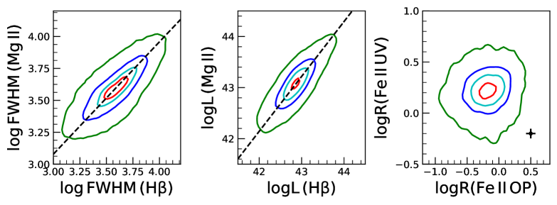
Figure 1: The relation between the FWHM (left) and luminosity (middle) of the Mg II line against the H$\beta$ line. The best fit relation is shown as dashed line. The flux ratio of UV Fe II (2200-3090 Å) to Mg II (R_FeII,UV) against the flux ratio of optical Fe II (4435-4685 Å) to H$\beta$ (R_FeII,OP) is shown in the right panel. The black symbol represents average error bar. The 20 (red), 40 (cyan), 68 (blue) and 95 (green) percentile density contours are shown in each panel.

3 Emission line properties in optical and UV

In Figure 1, we plot several correlations between H$\beta$ and Mg II line properties of 25,624 quasars for which both H$\beta$ and Mg II line information is available. We calculated the Spearman rank correlation coefficient ($r_{s}$) and null-hypothesis probability of no correlation ($p$-value) using Monte Carlo simulations of 10,000 iterations. In each iteration, first, data points were modified by a random Gaussian deviates of zero mean and standard deviation given by the measurement uncertainty and then performed the Spearman rank correlation test (see Curran, 2014). From the distribution of the results, we calculated the median value at 50 percentile and the lower and upper uncertainty at the 16 and 84 percentile, respectively. We find a strong positive correlation between H$\beta$ and Mg II line widths (left panel) with $r_{s}=0.698^{+0.002}_{-0.002}$ and $p<10^{-200}$. All the correlation results presented in this paper are given in Table 1.

From the linear regression analysis, we found that the line widths of Mg II and H$\beta$ lines are related as

$$\mathrm{\log FWHM\,(MgII)}=\alpha\times\mathrm{\log FWHM\,(H\beta)}+\beta$$ (1)

where $\alpha$ and $\beta$ values are given in Table 2. For this analysis, we used two other methods, (1) LINMIX code (Kelly, 2007), which is a Bayesian method using errors on both the axes and (2) BECS (Akritas & Bershady, 1996; Nemmen et al., 2012) which again is a linear regression method using measurement errors on both the axes. The BECS provides four sets of measurements which are mentioned in Table 2; (a) assuming X as the independent variable (Y$|$X), (b) assuming Y as the independent variable (X$|$Y), (c) line that bisects the Y$|$X and X$|$Y (Bisector) and (d) line that minimizes orthogonal distances (Orthogonal). All the methods provide a similar slope. As it is not clear which variable is independent, we, therefore, adopted the results obtained from the BCES Orthogonal method as the best result. However, depending on the method used, an upper limit of FWHM (H$\beta$)=2000 km s^-1 usually used to define NLS1 corresponds to a similar FWHM of Mg II line $\sim$2063-2315 km s^-1 (see Table 2). Such a strong correlation between FWHM of H$\beta$ and Mg II line has also been found by Kovačević-Dojčinović & Popović (2015) with the linear correlation coefficient $r=0.77$. Also, Jun et al. (2015) studied line width correlation for high-luminous and high-$z$ sources and found that the FWHM of Mg II could be a good substitute for FWHM H$\beta$ and this relation was not found to evolve with redshift or luminosity. Similarly, we found the luminosities of the Mg II and H$\beta$ lines to be strongly correlated (middle panel) having $r_{s}=0.791^{+0.001}_{-0.001}$ and $p<10^{-200}$ (see Table 1) as expected in a flux-limited sample. We also performed a linear regression analysis to the $\mathrm{\log L\,(MgII)}-\mathrm{\log L\,(H\beta)}$ diagram (Table 2). Both LINMIX and BCES (Orthogonal) provided a slope of unity.

Table 1: Spearman rank correlation analysis. Columns are (1) relation (2) correlation coefficient ($r_{s}$), (3-4) probability of no correlation ($p$-value) and 1$\sigma$ upper uncertainty (5) number of data points.

y vs x	$r_{s}$	$p$	+$e_{p}$	N
(1)	(2)	(3)	(4)	(5)
FWHM (Mg II) $-$ FWHM (H$\beta$)	$0.698^{+0.002}_{-0.002}$	$<10^{-200}$	$-$	25624
L (Mg II) $-$ L (H$\beta$)	$0.791^{+0.001}_{-0.001}$	$<10^{-200}$	$-$	25624
R(Fe II, UV) $-$ R(Fe II, OP)	$0.114^{+0.005}_{-0.005}$	${2\times 10^{-29}}$	$5\times 10^{-27}$	9584
FWHM (H$\beta$) $-$ EW (H$\beta$)	$0.130^{+0.004}_{-0.004}$	$6\times 10^{-98}$	$7\times 10^{-92}$	25624
FWHM(H$\beta$) $-$ EW (Fe II, OP)	$-0.294^{+0.005}_{-0.005}$	$1\times 10^{-190}$	$2\times 10^{-184}$	9584
FWHM (Mg II) $-$ EW (Mg II)	$0.347^{+0.003}_{-0.003}$	$<10^{-200}$	$-$	25624
FWHM (Mg II) $-$ EW (Fe II, UV)	$0.143^{+0.004}_{-0.004}$	$5\times 10^{-45}$	$9\times 10^{-43}$	9584

Table 2: Results of the correlation analysis (y = $\alpha$x+ $\beta$) between Mg II and H$\beta$ lines. The columns are as follows (1) y-axis variable, (2) x-axis variable, (3) method used to perform linear fit and (4)-(5) slope and intercept of the linear fit.

y	x	method	$\alpha$	$\beta$
(1)	(2)	(3)	(4)	(5)
log FWHM(Mg II)	log FWHM (H$\beta$)	LINMIX	$0.792\pm 0.004$	$0.750\pm 0.012$
		BCES (Y$|$X)	$0.812\pm 0.005$	$0.681\pm 0.018$
		BCES (Y$|$X)	$0.975\pm 0.007$	$0.096\pm 0.026$
		BCES (Bisector)	$0.890\pm 0.005$	$0.401\pm 0.017$
		BCES (Orthogonal)	$0.880\pm 0.005$	$0.438\pm 0.018$
log L(Mg II)	log L (H$\beta$)	LINMIX	$0.888\pm 0.004$	$4.998\pm 0.159$
		BCES (Y$|$X)	$0.897\pm 0.004$	$4.593\pm 0.171$
		BCES (X$|$Y)	$1.258\pm 0.006$	$-10.881\pm 0.270$
		BCES (Bisector)	$1.062\pm 0.004$	$-2.452\pm 0.174$
		BCES (Orthogonal)	$1.074\pm 0.005$	$-3.006\pm 0.213$

NLS1 shows stronger Fe II emission in the optical compared to the BLS1 (Rakshit et al., 2017). To find out any correlation between optical and UV Fe II strength, we plot the optical Fe II strength ($R_{\mathrm{FeII,OP}}$) which is the ratio of the EW of Fe II in the wavelength range of $4435-4685$ Å  to the H$\beta$ against the UV Fe II strength ($R_{\mathrm{FeII,UV}}$) which is the ratio of the EW of Fe II in the wavelength range $2200-3090$ Å  to the Mg II in the right panel of Figure 1. A weak but positive correlation between them with $r_{s}=0.114^{+0.005}_{-0.005}$ and $p=2\times 10^{-29}$ is present albeit with large dispersion.

From principal component analysis (PCA) of a sample of PG quasars Boroson & Green (1992) found that the first eigenvector (EV1), which explains the difference between various AGN types, is dominated by the strong anti-correlation between the strength of Fe II and [O III]5007 as well as radio-loudness, H$\beta$ FWHM and asymmetry. The optical plane of EV1 correlation involves two main parameters, FWHM of H$\beta$ and the strength of Fe II to H$\beta$ (Sulentic et al., 2000). The main driver of EV1 is believed to be the orientation and Eddington ratio (Shen & Ho, 2014). The former strongly affects the line kinematics and particularly important for objects having flat broad line region (BLR) geometry while the latter is found to be strongly correlated with the Fe II strength. The NLS1s, by definition, are located at the lower part of the EV1 diagram (e.g., Rakshit et al., 2017). To find out any similarities of the optical plane of EV1 with the UV plane of EV1, in Figure 2, we plot line FWHM against $R_{\mathrm{FeII}}$ in the optical and UV. The FWHM (H$\beta$) v/s. $R_{\mathrm{FeII,OP}}$ is shown in red while FWHM (Mg II) v/s $R_{\mathrm{FeII,UV}}$ is shown in blue. We do see a similar shape in both optical and UV EV1 diagrams.

As shown in Figure 3, the shape of EV1 in UV is dominated by the strong positive correlation ($r_{s}=0.347^{+0.003}_{-0.003}$) between the FWHM and EW of Mg II, since the EW of UV Fe II is weakly correlated ($r_{s}=0.143^{+0.004}_{-0.004}$) with the FWHM of Mg II (see Table 1). While in the optical, the FWHM of H$\beta$ is weekly correlated ($r_{s}=0.130^{+0.004}_{-0.004}$) with its EW, the EW of Fe II in the optical is anti-correlated ($r_{s}=-0.294^{+0.005}_{-0.005}$) with the FWHM of H$\beta$. Such differences between UV and optical Fe II lines have been noticed by Kovačević-Dojčinović & Popović (2015). The differences could be due to different spatial distribution of clouds in the emitting region and/or the different excitation mechanisms. For example, Ferland et al. (2009) suggested that the cloud distribution of the UV Fe II is asymmetric while for optical Fe II line they are isotropic (see Sameshima et al., 2011). Indeed Kovačević-Dojčinović & Popović (2015) found that although the UV and optical lines originate around the similar region in AGN, The UV Fe II emitting clouds have asymmetric distribution while the optical Fe II clouds have isotropic distribution. On the other hand, different excitation mechanisms could be responsible for the optical and UV Fe II emission. The optical depth of UV Fe II is larger than the optical Fe II, hence UV Fe II lines decrease more rapidly than the optical Fe II with the increase of column density (Joly, 1987).

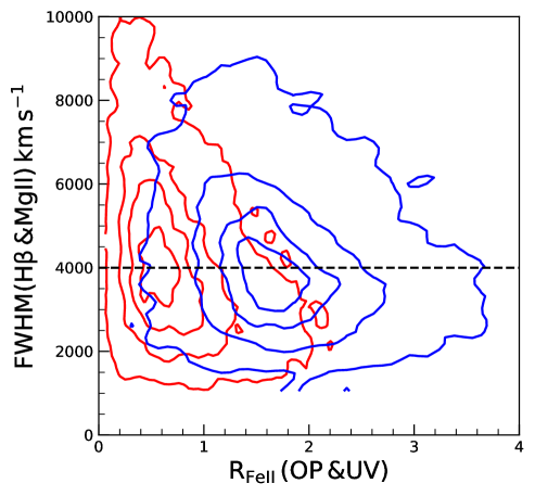
Figure 2: Relation between the line width of H$\beta$ against the optical Fe II strength R_FeII,OP (red contours) and Mg II line width against the UV Fe II strength R_FeII,UV (blue). The 20, 40, 68 and 95 percentile density contours are shown from inner to outer.

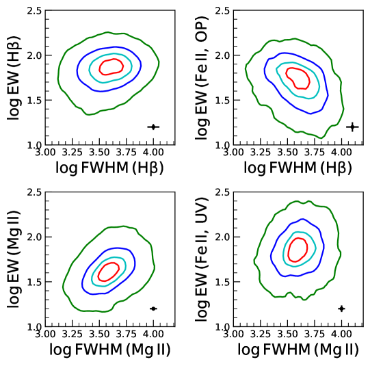
Figure 3: Top panels: H$\beta$ and Optical Fe II line EW are plotted against the FWHM of H$\beta$. Bottom panels: Mg II and UV Fe II line EW are plotted against the FWHM of Mg II. The black symbol in each panel represents the average error bar. The 20 (red), 40 (cyan), 68 (blue) and 95 (green) percentile density contours are shown.

4 high-z NLS1 candidates

Since NLS1s are classified based on the criteria of FWHM(H$\beta)<2000$ km s^-1, and [O III]/H$\beta<3$, one can use the correlation between Mg II and H$\beta$ line width to select high-$z$ NLS1s when the H$\beta$ line is not present. We, therefore, selected an object to be a NLS1 if the FWHM of the Mg II line is $<2000$ km s^-1. We note that the classical definition of NLS1 is subjective and has been debated since the broad line widths do not show any bimodality or discontinuity. A more conservative limit at FWHM(H$\beta$)=4000 km s^-1 has been suggested where sources below 4000 km s^-1 are termed as population A while above 4000 km s^-1 are termed as population B based on the optical plane of EV1 diagram (Sulentic et al., 2000; Marziani et al., 2018). Here, NLS1s fall under population A. Moreover, many NLS1s are found to be very weak Fe II emitters. Thus, Zhou et al. (2006) and Rakshit et al. (2017) used a cutoff of 2200 km s^-1 slightly larger than 2000 km s^-1. A larger FWHM increases the sample, however, the average black hole mass of the same also increases. On the other hand Netzer & Trakhtenbrot (2007) suggested using the Eddington ratio cutoff of $L/L_{\mathrm{Edd}}\geq 0.25$.

The [O III]/H$\beta<3$ criterion mainly separate NLS1s from Type 2 AGN in the low-resolution and low-SNR spectra since line fluxes are difficult to measure (see Halpern et al., 1999, 1998). This is not the case in our study as we restricted our sample with strong emission lines. Also, this flux ratio criterion has been excluded when high ionization iron lines, e.g., [Fe vii] k6087 and [Fe x] k6375 are present (exception, for example, IC 3599; Véron-Cetty et al., 2001). Since all of our objects have broad line width larger than 900 km s^-1, larger than Type 2 AGN and are quasars based on the absolute magnitude, we ignore the flux ratio criterion. With the above conditions, we obtain a sample of 2684 high-$z$ NLS1 candidates. The catalog of high-$z$ NLS1 candidates is available on Zenodo (doi:10.5281/zenodo.4405039) and column information are given in Table 3. Note that measurements are directly taken from R20.

To study the high-$z$ NLS1 properties, we also compare it with the low-$z$ NLS1 sample ($z<0.8$) present in the DR 14 quasar catalog. This low-$z$ sample, which is selected as per the classical definition of FWHM (H$\beta$) $<2000$ km s^-1 and [O III]/H$\beta<3$ has 3109 NLS1. If we exclude the flux ratio criterion, we found 3131 sources. This suggests the flux ratio criterion is not important in our selection of high-$z$ NLS1s.

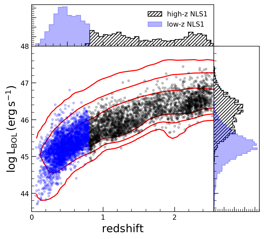
Figure 4: The bolometric luminosity against redshift. The low-z NLS1 (blue) and high-z NLS1 candidates (black) are shown along with the parent sample (1$\sigma$, 2$\sigma$, 3$\sigma$ density contours) of SDSS DR14 quasars. The top and right panels show the distribution of redshift and bolometric luminosity, respectively for NLS1.

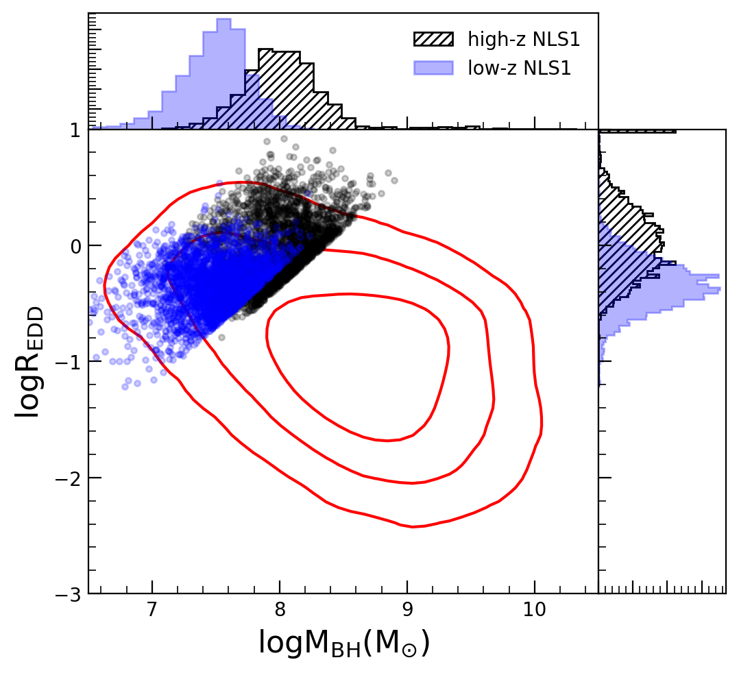
Figure 5: The Eddington ratio is plotted against black hole mass for low-z NLS1 (blue), high-z NLS1 candidates (black dots) along with the SDSS DR14 quasars for $z<2.2$ (1$\sigma$, 2$\sigma$, and 3$\sigma$ density contours). The histograms of black hole mass (top panel) and Eddington ratio (right panel) are also shown.

Table 3: High-z NLS1 catalog. Columns are (1) FITS column number, (2) name of the column, (3) format (4) unit, and (5) description. All the quantities are directly taken from R20.

Number	Column Name	Format	Unit	Description
(1)	(2)	(3)	(4)	(5)
1	SDSS_NAME	String		40cmObject name as given in R20.
2	RA	Double	Degree	Right Ascension (J2000)
3	DEC	Double	Degree	Declination (J2000)
4	SDSS_ID	String		PLATE-MJD-FIBER
5	REDSHIFT	Double		Redshift
6	LOG_L3000	Double	erg s-1	Logarithmic continuum luminosity at rest-frame 3000 Å
7	LOG_L3000_ERR	Double	erg s-1	Measurement error in LOG_L3000
8	FWHM_MGII_BR	Double	km s-1	FWHM of Mg II broad component
9	FWHM_MGII_BR_ERR	Double	km s-1	Measurement error in FWHM_MGII_BR
10	EW_MGII_BR	Double	Å	Rest-frame equivalent width of Mg II broad component
11	EW_MGII_BR_ERR	Double	Å	Measurement error in EW_MGII_BR
12	LOGL_MGII_BR	Double	erg s-1	Logarithmic line luminosity of Mg II broad component
13	LOGL_MGII_BR_ERR	Double	erg s-1	Measurement error in LOGL_MGII_BR
14	LOGL_MGII_NA	Double	erg s-1	Logarithmic line luminosity of Mg II narrow component
15	LOGL_MGII_NA_ERR	Double	erg s-1	Measurement error in LOGL_MGII_NA
16	LOGL_FE_UV	Double	erg s-1	40cmLogarithmic luminosity of the UV Fe II complex
within the 2200-3090 Å
17	LOGL_FE_UV_ERR	Double	erg s-1	Measurement error in LOGL_FE_UV
18	EW_FE_UV	Double	Å	40cmRest-frame equivalent width of UV Fe II complex
within the 2200-3090 Å
19	EW_FE_UV_ERR	Double	Å	Measurement error in EW_FE_UV
20	LOG_MBH	Double	$M_{\odot}$	Logarithmic fiducial single-epoch BH mass
21	LOG_MBH_ERR	Double	$M_{\odot}$	Measurement error in LOG_MBH
22	LOG_REDD	Double		40cmLogarithmic Eddington ratio based on
fiducial single-epoch BH mass

Table 4: Spearman rank correlation analysis. Columns are (1) relation (2) sample (3) name of data points (4) correlation coefficient ($r_{s}$), (5-6) probability of no correlation ($p$-value) and 1$\sigma$ upper uncertainty.

y vs x	sample	N	$r_{s}$	$p$	+$e_{p}$
(1)	(2)	(3)	(4)	(5)	(6)
R(Fe II, UV) vs. $R_{\mathrm{EDD}}$	high-z NLS1	2002	$0.077^{+0.019}_{-0.019}$	$5\times 10^{-4}$	$9\times 10^{-3}$
R(Fe II, OP) vs. $R_{\mathrm{EDD}}$	low-z NLS1	2917	$0.095^{+0.014}_{-0.014}$	$2\times 10^{-7}$	$9\times 10^{-6}$
R(Fe II, UV) vs. $R_{\mathrm{EDD}}$	DR14 quasars	115354	$0.237^{+0.001}_{-0.001}$	$<10^{-200}$	–
R(Fe II, OP) vs. $R_{\mathrm{EDD}}$	DR14 quasars	28577	$0.361^{+0.002}_{-0.002}$	$<10^{-200}$	–
EW(Fe II, OP)/EW(Fe II, UV) vs. $R_{\mathrm{EDD}}$	DR14 quasars	9584	$0.282^{+0.004}_{-0.004}$	$3\times 10^{-175}$	$9\times 10^{-170}$
$R_{1.4}$ vs. $L_{1.4}$	high-z NLS1	130	$0.800^{+0.003}_{-0.003}$	$3\times 10^{-30}$	$3\times 5^{-30}$
$R_{1.4}$ vs. $L_{1.4}$	low-z NLS1	187	$0.727^{+0.005}_{-0.005}$	$4\times 10^{-32}$	$1\times 10^{-31}$
$R_{1.4}$ vs. $L_{1.4}$	DR14 quasars	18236	$0.778^{+0.001}_{-0.001}$	$<10^{-200}$	$--$
$M_{BH}$ vs. $L_{1.4}$	high-z NLS1	130	$0.394^{+0.048}_{-0.049}$	$3\times 10^{-6}$	$5\times 10^{-5}$
$M_{BH}$ vs. $L_{1.4}$	low-z NLS1	187	$0.313^{+0.042}_{-0.043}$	$1\times 10^{-5}$	$2\times 10^{-4}$
$M_{BH}$ vs. $L_{1.4}$	All NLS1	317	$0.596^{+0.023}_{-0.022}$	$5\times 10^{-32}$	$3\times 10^{-29}$
$M_{BH}$ vs. $L_{1.4}$	DR14 quasars ($z<2.2$)	10437	$0.218^{+0.003}_{-0.003}$	$5\times 10^{-113}$	$1\times 10^{-109}$

5 Properties of high-z NLS1

We used the values of the bolometric luminosities from R20, who measured them from the monochromatic luminosities after applying the corresponding bolometric corrections. In Figure 4, we plot the bolometric luminosities against redshifts for the low-$z$ NLS1s (blue) and high-$z$ NLS1 candidates (black). In the same figure, the density contours of SDSS DR14 quasars are also shown. The median $\log L_{\mathrm{bol}}$ for low-$z$ and high-$z$ NLS1 candidates are found to be $45.29\pm 0.39$ erg s^-1 and $46.16\pm 0.42$ erg s^-1, respectively. Their redshift distribution ranges from $0.06-0.8$ for low-z NLS1s and $0.8-2.57$ for high-$z$ NLS1s.

R20 provided fiducial virial black hole masses based on H$\beta$ (for $z<0.8$), Mg II (for $0.8\leq z<1.9$) and CIV (for $z\geq 1.9$) lines depending on the redshift with decreasing preference from H$\beta$ to CIV. They also estimated the Eddington ratio, which is the ratio of bolometric to Eddington luminosity where the former is based on the continuum luminosity with the appropriate bolometric correction factor and the latter is based on the black hole masses. We used the measurements provided in R20. Note that for $z>1.9$ sources, the fiducial virial masses are based on CIV line and they tend to have larger uncertainties than Mg II masses (e.g., Denney, 2012; Trakhtenbrot & Netzer, 2012; Park et al., 2017; Rakshit et al., 2020). Hence many of the high-$z$ NLS1 in the redshift range of $z>1.9$, for which R20 provides Mg II based masses, we used them instead of the fiducial masses.

In Figure 5, we plot the distribution of $M_{\mathrm{BH}}$ values and Eddington ratios for the low-z NLS1s (blue-dots) and high-$z$ NLS1 candidates (black-dots). They are also shown in the $M_{\mathrm{BH}}$ versus Eddington ratio plane. We also plot the density contours (1$\sigma$, 2$\sigma$, 3$\sigma$) of SDSS DR14 quasars for $z<2.2$. The NLS1s are located at the extreme upper left corner of the diagram having low black hole mass and higher Eddington ratio. The median logarithmic black hole mass of high-$z$ NLS1 candidates is $8.01\pm 0.35\,M_{\odot}$ slightly larger than the sample of low-z NLS1s ($7.51\pm 0.27\,M_{\odot}$). The higher mass of the high-z NLS1 sample is due to the higher luminosity compared to the low-z NLS1 sample. However, this is much lower compared to the overall sample of SDSS DR14 quasars up to $z<2.2$, which is $8.64\pm 0.50\,M_{\odot}$. Similarly, the logarithmic Eddington ratio distribution has a median of $0.02\pm 0.27$ and $-0.35\pm 0.21$ for high-$z$ and low-$z$ NLS1s, respectively. These values are much higher than that of SDSS DR14 quasars that have a median value of $-0.96\pm 0.43$ up to $z<2.2$.

In Figure 6, we plot the Eddington ratio as a function of Fe II strength in optical (left) and UV (right). We also plotted the density contours of SDSS DR14 quasars. The NLS1 candidates are located at the extreme upper right corner of the diagram. A moderately strong correlation between Fe II strength and Eddington ratio is found having $r_{s}=0.361^{+0.002}_{-0.002}$ in the optical and $0.237^{+0.001}_{-0.001}$ in the UV for SDSS DR14 quasars (see Table 4). This positive correlation is also present in the low-z and high-z NLS1 samples but very weak due to the small range of the Eddington ratio of these samples. A positive correlation between Fe II strength and Eddington ratio is known to exist e.g., Negrete et al. (2018) using a sample of 302 high accreting sources found a positive correlation with a correlation coefficient of $0.49$ between the optical Fe II strength and Eddington ratio similar to what has been found here. Moreover, using a SDSS sample, Shin et al. (2019) found a positive correlation with a correlation coefficient of 0.48 between UV Fe II strength and Eddington ratio. In fact, the ratio of the equivalent width of optical to UV Fe II increases with the Eddington ratio having $r_{s}=0.282^{+0.004}_{-0.004}$ considering the SDSS DR14 quasars. Such a positive correlation but somewhat stronger has been found by Sameshima et al. (2011) using a sample of about 900 SDSS quasars from SDSS DR5. A dense medium and large column density is found for high accreting sources since lower density and small column density clouds could be blown away due to strong radiation pressure (see Dong et al., 2009). However, Netzer et al. (2004) suggested that increasing star formation could also lead to high density and large column density region. A high star formation rate in high Eddington ratio and low mass sources which are typically NLS1s is indeed found by Sani et al. (2010).

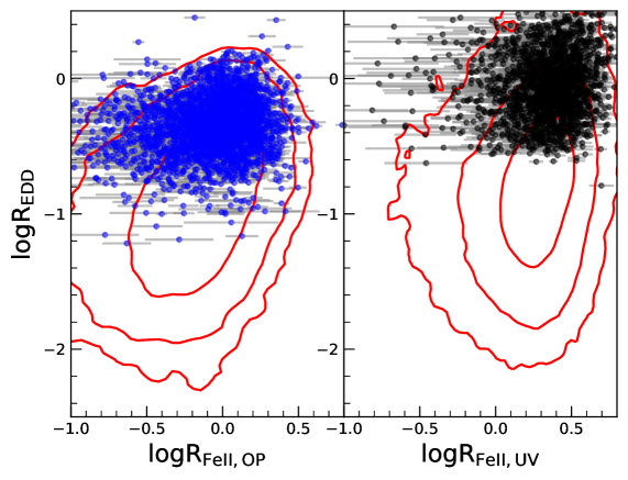
Figure 6: Eddington ratio is plotted against R_FeII,OP (left) while R_FeII,UV (blue). A positive correlation is noticed. The SDSS DR14 quasars are also shown by the solid contours (1$\sigma$, 2$\sigma$, and 3$\sigma$).

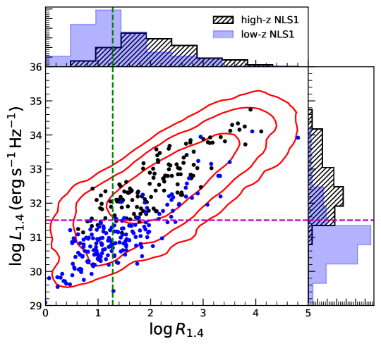
Figure 7: The 1.4 GHz radio luminosity against radio loudness. The blue and black circles are the low-$z$ and high-$z$ NLS1 candidates respectively. The 1$\sigma$, 2$\sigma$, and 3$\sigma$ density contours of DR14 quasars are shown in red. The vertical line at $R_{1.4}=19$ is the dividing line for the radio-quiet and radio-loud quasars while the horizontal line is the separation for FR I and II objects. The distributions of the radio loudness parameter and the radio luminosity at 1.4 GHz are also shown.

5.1 Radio properties

NLS1s are usually radio-quiet having a low radio detection fraction of about 5% (Komossa et al., 2006; Rakshit et al., 2017; Singh & Chand, 2018). The radio-loud fraction is even smaller, about 2.5%. A fraction of these sources are found to have large kpc-scale jet as well as high energy $\gamma$-ray emission (see Paliya et al., 2018, and references therein). The radio-detection fraction of NLS1s is much lower compared to the fraction of typical quasars (Kellermann et al., 1989). Pâris et al. (2018) cross-matched SDSS DR14 quasars with the 1.4GHz FIRST radio survey (catalog December 2014; Becker et al., 1995) with a radius of 2^′′ finding a total of 18,273 counterparts. This radio detection fraction, only 4% of SDSS DR14 quasars, is much smaller than the 16% found in earlier studies (e.g., Kellermann et al., 1989). If we consider sources with continuum S/N $>5$ pixel^-1, a similar low radio detection is found, only 6%. However, this fraction is limited by the sensitivity of the FIRST survey which is 1 mJy/beam. Indeed, at low redshift $z<0.3$, the detection fraction is found to be 16% as usually considered, however, it decreases to 8% for $z<0.8$. The detection fraction of our low-$z$ NLS1 sample is 7% while for the high-z NLS1 candidate sample it is 6%. Thus, the fraction of radio detected NLS1s is similar to the SDSS DR 14 quasars fraction and strongly depends on the redshift and the flux limit of the radio survey.

To study the radio properties of the high-redshift NLS1 candidates, we calculated the 1.4 GHz luminosity ($L_{\mathrm{1.4GHz}}$) from the integrated sources flux after k-correction assuming a radio spectral index $\alpha=0$ i.e the measured radio flux divided by (1+z) (see Donoso et al., 2009). The radio loudness $R_{\mathrm{1.4GHz}}$ was calculated by the ratio of integrated radio flux to the optical SDSS g-band flux. In Figure 7 we plot $L_{\mathrm{1.4GHz}}$ against $R_{\mathrm{1.4GHz}}$. The distribution of low-$z$ and high-$z$ NLS1s along both the axes are shown. The vertical line represents the division of FR I and FR II sources (Fanaroff & Riley, 1974), while the horizontal line at $R_{\mathrm{1.4GHz}}=19$ represents the dividing line between radio-quiet and radio-loud sources based on the 1.4GHz radio flux (Komossa et al., 2006; Singh & Chand, 2018) which corresponds to the original dividing line of $R=10$ based on the 5 GHz radio flux (Kellermann et al., 1989).

Figure 7 shows a strong positive correlation ($r_{s}=0.778^{+0.001}_{-0.001}$) between radio luminosity and the radio loudness which is expected as the latter is the radio flux normalized by the optical flux. The dispersion in the relationship could be due to the differences in intrinsic AGN parameters, e.g., black hole mass, accretion process, etc. Such a strong positive correlation is found to be present in both high-z NLS1 ($r_{s}=0.800^{+0.003}_{-0.003}$) and low-z NLS1 samples ($r_{s}=0.727^{+0.005}_{-0.005}$), which agrees with the previous finding on low-z NLS1 sample (e.g., Singh & Chand, 2018). The radio-loudness of our high-$z$ sample ranges from $4-10^{4.1}$ with a median of 99, while for the low-$z$ sample the range is $1-10^{4.8}$ with a median of 17. The fraction of RL source is found to be similar (4.2%) in the high-$z$ NLS1 sample and the low-$z$ NLS1 (2.8%). The radio-luminosities of our high-$z$ sample range from $10^{31.1}-10^{34.7}$ erg s^-1 Hz^-1 with a median of $10^{32.4}$ erg s^-1 Hz^-1, much larger than the low-z sample, that ranges from $10^{29.1}-10^{34.1}$ erg s^-1 Hz^-1 with a median of $10^{30.9}$ erg s^-1 Hz^-1. The low-$z$ sample, which is mostly radio-quiet also has much lower radio-power and belongs to FR I, while high-$z$ NLS1s are mostly radio-loud with powerful radio jets and belongs to the FR II category.

We do not find any evidence for bimodality both in the NLS1 sample as well as in the parent sample of SDSS quasars. This is in contrast to the earlier reports on radio-loud and radio-quiet dichotomy (Kellermann et al., 1989), however, our results agree with the previous findings which are based on a large sample (Rafter et al., 2008; Rakshit et al., 2018a; Singh & Chand, 2018). The presence of bimodality in the earlier studies could be due to sample selection biases e.g., host galaxy type such as the radio-loud sources being hosted in giant elliptical and radio-quiet sources being hosted in spiral galaxies (Sikora et al., 2007). Also, such bimodality may not be present if the nuclear radio emission is smoothly correlated with the AGN properties, such as black hole mass and Eddington ratio, as already found by Laor (2000) and Lacy et al. (2001). Indeed we found the radio luminosity to be strongly correlated with black hole mass (see Figure 8) having $r_{s}=0.596^{+0.023}_{-0.022}$ for the NLS1s (including low-$z$ and high-$z$). This correlation is also present separately in the low-$z$ ($r_{s}=0.313^{+0.042}_{-0.043}$) and high-$z$ NLS1 samples ($r_{s}=0.394^{+0.048}_{-0.049}$) though a little weaker due to the sample range since high-$z$ radio detected NLS1s have in general black holes mass of about $10^{8}M_{\odot}$. Moreover, the positive correlation between radio-power and black hole mass is also present albeit with a large dispersion ($r_{s}=0.218^{+0.003}_{-0.003}$) in the parent SDSS DR14 quasars sample supporting the finding of Laor (2000). Lacy et al. (2001) found this correlation to be tighter when the Eddington ratio is also considered along with black hole masses, however, the dependency is weaker at a low Eddington ratio. Since our NLS1s are drawn from the parent SDSS DR14 quasars sample and have a higher Eddington ratio, a tighter correlation in the former compared to the latter is thus expected.

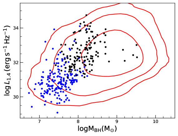
Figure 8: The 1.4GHz radio luminosity is plotted against black hole mass from low-z (blue filled circles), high-z (black filled circles) and SDSS DR14 quasars for $z<2.2$ (as contours in red).

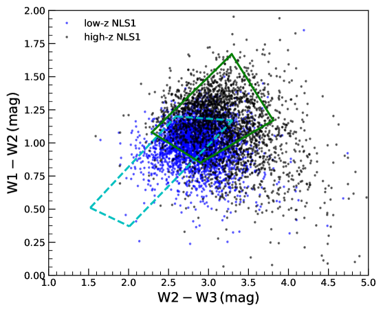
Figure 9: WISE W1-W2 color vs W2-W3 color diagram for NLS1s. Filled blue and black circles are the low-$z$ and high-$z$ NLS1s respectively. The location of the WISE $\gamma$-ray strips for FSRQ (solid green) and BL Lacs (dashed-cyan) are also shown.

5.2 color-color diagram

In Rakshit et al. (2019), we studied the infrared color and variability of low-$z$ NLS1s from SDSS DR12 using photometry magnitude from WISE. We found 57.6% of the variable NLS1s are situated in the WISE color-color diagram, while 30% are within the WISE $\gamma$-ray strip of BL Lac and FSRQs. To study the IR properties, we used the compilation of Pâris et al. (2018) and R20, where SDSS DR14 quasars were cross-matched with the AllWISE Source catalog (Wright et al., 2010) with a matching radius of 2^′′. About 92% and 98% of our high-$z$ and low-$z$ NLS1s, respectively, have WISE counterpart. In Figure 9, we plot the WISE W1-W2 color against W2-W3 color for the low-$z$ NLS1 (blue) and high-$z$ NLS1 (black) candidates. The mean W1-W2 color of high-$z$ (low-$z$) NLS1s is found to be $1.14\pm 0.26$ ($1.00\pm 0.16$), while W2-W3 color is $3.18\pm 0.44$ ($2.86\pm 0.31$).

About 77% of low-$z$ and 61% of high-$z$ BLS1s lie in the region occupied by WISE $\gamma$-ray strip. About 60% (16%) of high-$z$ NLS1s are located in the region occupied by FSRQs (BL Lacs), among them, 15% are common to BL Lac and FSRQs, while the same for the low-$z$ NLS1 sample is found to be 65% (57%) among which 45% are common to both. Thus, based on the IR color-color diagram, it is evident that most of our NLS1 galaxies have blazar like properties and are AGN as expected since they are optically selected quasars with broad emission lines.

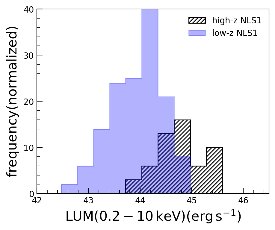
Figure 10: The soft X-ray 0.2-10 keV luminosity distribution of low-$z$ and high-$z$ NLS1s.

5.3 X-ray properties

The steep soft X-ray spectra and soft X-ray access are the main characteristics of NLS1 galaxies. Recently, Ojha et al. (2020) performed soft and hard X-ray spectral analysis of a large sample of NLS1 and BLS1 using the low-$z$ sample of Rakshit et al. (2017). They found that the X-ray photon index strongly correlates with the Eddington ratio and R_FeII. It is also found to be anti-correlated with line width. R20 culled multi-band properties of SDSS DR14 quasars from Pâris et al. (2018) who cross-matched SDSS DR14 quasars with the Third XMM-Newton Serendipitous Source Catalog (3XMM-DR7; Rosen et al., 2016) using a standard 5.0^′′ matching radius.

To investigate the X-ray properties of high-$z$ NLS1, we used these values. Among the low-$z$ NLS1 sources having $z<0.8$, 141 are present in 3XMM-DR7, while only 54 of the high-z NLS1 candidates are present. In Figure 10, we plot the soft X-ray (0.2-10 keV) luminosity of the sample. The median $\log L_{0.2-10}$ keV of high-$z$ (low-$z$) NLS1 candidate is found to be $44.78\pm 0.43$ ($44.03\pm 0.49$) erg s^-1.

We also cross-correlated the DR14 quasar spectral catalog of R20 with the ROSAT all-sky survey (2RXS) source catalog (Boller et al., 2016) within a search radius of 30^′′ and found 8,658 detections. The 2RXS catalog provides photon index from power-law spectral fitting that can be used to study the correlation of photo index with the emission line width. In Figure 11, we plot soft X-ray (0.1-2 KeV) ROSAT photon index as a function of FWHM of H$\beta$ (left) and Mg II (right) for 459 and 143 sources, respectively, that have at least 50 source counts and photon index measurements better than 1$\sigma$. Note that the average uncertainty of ROSAT photon index is 50%. We find a general trend of decreasing photon index with increasing line width, both for H$\beta$ and Mg II line with $r_{s}=-0.30$ and $r_{s}=-0.31$, respectively. This is consistent with the fact of low-z NLS1s having a higher photon index compared to the BLS1s found in previous studies (e.g., Boller et al., 1996; Ojha et al., 2020). The anti-correlation of photon index with FWHM(Mg II) suggests that the latter is a good proxy for FWHM(H$\beta$) for selecting high-z NLS1s.

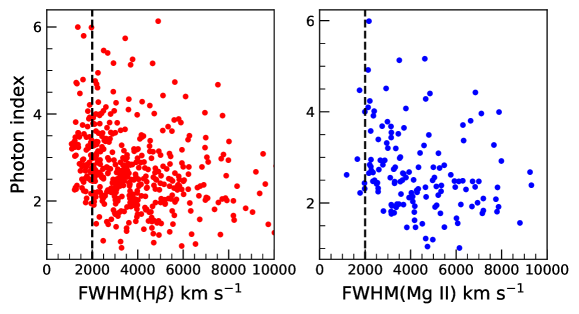
Figure 11: The ROSAT soft X-ray (0.1-2 KeV) photon index is plotted against FWHM (H$\beta$) and FWHM(Mg II). The vertical line at FWHM=2000 km s^-1 represents the division of NLS1 from BLS1.

6 Summary

Our knowledge of the general physical properties of NLS1s are based on NLS1s available up to $z$ = 0.8. This is mainly constrained by the definition of NLS1s that requires the presence of H$\beta$ emission line, which is only available in large optical spectroscopic surveys up to sources with $z<0.8$. To find out high-$z$ NLS1 candidates, we studied H$\beta$ and Mg II line properties of a large number of SDSS DR14 quasars using the spectral properties cataloged by R20. We found that the UV EV1 has a similar shape as the optical plane of EV1 which are believed to be the main driver of the quasars spectral properties. The shape of UV EV1 is due to the strong correlation between the EW and FWHM of Mg II line while the shape of optical EV1 is due to the strong anti-correlation between the EW of Fe II in the optical against the FWMH of H$\beta$. A strong correlation between Mg II and H$\beta$ line FWHM is also found which allowed us to provide a sample of high-$z$ NLS1 based on Mg II FWHM $<2000$ km s^-1.

We supplemented this work with a low-$z$ NLS1 sample based on the H$\beta$ line as per the classical definition. The high-$z$ NLS1 sample has a redshift range of $0.8-2.5$ and median logarithmic bolometric luminosity of $46.16\pm 0.42$ erg s^-1 larger than the median logarithmic bolometric luminosity of $45.29\pm 0.39$ erg s^-1 found for the low-z sample. The median logarithmic black hole mass of the sample is $8.01\pm 0.35$ $M_{\odot}$ and logarithmic Eddington ratio is $0.02\pm 0.27$. The black hole mass and Eddington ratio of the high-$z$ NLS1 is slightly higher and lower, respectively, compared to the low-$z$ sample due to the higher median bolometric luminosity in the former but compared to the parent SDSS Dr14 quasar sample, the black hole mass is much lower and the Eddington ratio is much higher.

The radio detection rate of high-$z$ and low-$z$ samples are similar to the SDSS DR14 quasars at a similar redshift range. The high-$z$ NLS1 sources are mainly FR II type sources having powerful jets compared to their low-z NLS1 counterparts which seem to be due to their higher black hole mass since a strong correlation between 1.4GHz radio luminosity and black hole mass has been found. A major fraction of them is located within the WISE $\gamma$-ray strip similar to the low-$z$ NLS1s confirming their AGN nature. This catalog will be immensely useful to the community in studies of high-z NLS1s e.g., comparison with BLS1s, and the search for high-z $\gamma$-ray emitters.

References

- Akritas & Bershady (1996) Akritas, M. G., & Bershady, M. A. 1996, ApJ, 470, 706
- Baldi et al. (2016) Baldi, R. D., Capetti, A., Robinson, A., Laor, A., & Behar, E. 2016, MNRAS, 458, L69
- Becker et al. (1995) Becker, R. H., White, R. L., & Helfand, D. J. 1995, ApJ, 450, 559
- Boller et al. (1996) Boller, T., Brandt, W. N., & Fink, H. 1996, A&A, 305, 53
- Boller et al. (2016) Boller, T., Freyberg, M. J., Trümper, J., et al. 2016, A&A, 588, A103
- Boroson & Green (1992) Boroson, T. A., & Green, R. F. 1992, ApJS, 80, 109
- Calderone et al. (2013) Calderone, G., Ghisellini, G., Colpi, M., & Dotti, M. 2013, MNRAS, 431, 210
- Chen et al. (2018) Chen, S., Berton, M., La Mura, G., et al. 2018, A&A, 615, A167
- Curran (2014) Curran, P. A. 2014, arXiv e-prints, arXiv:1411.3816
- Decarli et al. (2008) Decarli, R., Dotti, M., Fontana, M., & Haardt, F. 2008, MNRAS, 386, L15
- Denney (2012) Denney, K. D. 2012, ApJ, 759, 44
- Dong et al. (2009) Dong, X.-B., Wang, T.-G., Wang, J.-G., et al. 2009, ApJ, 703, L1
- Donoso et al. (2009) Donoso, E., Best, P. N., & Kauffmann, G. 2009, MNRAS, 392, 617
- Fanaroff & Riley (1974) Fanaroff, B. L., & Riley, J. M. 1974, MNRAS, 167, 31P
- Ferland et al. (2009) Ferland, G. J., Hu, C., Wang, J.-M., et al. 2009, The Astrophysical Journal, 707, L82
- Goodrich (1989) Goodrich, R. W. 1989, ApJ, 342, 224
- Grupe (2000) Grupe, D. 2000, New A Rev., 44, 455
- Grupe & Mathur (2004) Grupe, D., & Mathur, S. 2004, ApJ, 606, L41
- Guo et al. (2018) Guo, H., Shen, Y., & Wang, S. 2018, PyQSOFit: Python code to fit the spectrum of quasars, Astrophysics Source Code Library, ascl:1809.008
- Halpern et al. (1998) Halpern, J. P., Eracleous, M., & Forster, K. 1998, ApJ, 501, 103
- Halpern & Moran (1998) Halpern, J. P., & Moran, E. C. 1998, ApJ, 494, 194
- Halpern et al. (1999) Halpern, J. P., Turner, T. J., & George, I. M. 1999, MNRAS, 307, L47
- Järvelä et al. (2018) Järvelä, E., Lähteenmäki, A., & Berton, M. 2018, A&A, 619, A69
- Joly (1987) Joly, M. 1987, A&A, 184, 33
- Jun et al. (2015) Jun, H. D., Im, M., Lee, H. M., et al. 2015, ApJ, 806, 109
- Kellermann et al. (1989) Kellermann, K. I., Sramek, R., Schmidt, M., Shaffer, D. B., & Green, R. 1989, AJ, 98, 1195
- Kelly (2007) Kelly, B. C. 2007, ApJ, 665, 1489
- Komossa et al. (2006) Komossa, S., Voges, W., Xu, D., et al. 2006, AJ, 132, 531
- Kovačević-Dojčinović & Popović (2015) Kovačević-Dojčinović, J., & Popović, L. Č. 2015, ApJS, 221, 35
- Lacy et al. (2001) Lacy, M., Laurent-Muehleisen, S. A., Ridgway, S. E., Becker, R. H., & White, R. L. 2001, The Astrophysical Journal, 551, L17
- Laor (2000) Laor, A. 2000, The Astrophysical Journal, 543, L111
- Leighly (1999) Leighly, K. M. 1999, ApJS, 125, 317
- Marziani et al. (2018) Marziani, P., Dultzin, D., Sulentic, J. W., et al. 2018, Frontiers in Astronomy and Space Sciences, 5, 6
- Mathur (2000) Mathur, S. 2000, MNRAS, 314, L17
- Nandra & Pounds (1994) Nandra, K., & Pounds, K. A. 1994, MNRAS, 268, 405
- Negrete et al. (2018) Negrete, C. A., Dultzin, D., Marziani, P., et al. 2018, A&A, 620, A118
- Nemmen et al. (2012) Nemmen, R. S., Georganopoulos, M., Guiriec, S., et al. 2012, Science, 338, 1445
- Netzer et al. (2004) Netzer, H., Shemmer, O., Maiolino, R., et al. 2004, ApJ, 614, 558
- Netzer & Trakhtenbrot (2007) Netzer, H., & Trakhtenbrot, B. 2007, ApJ, 654, 754
- Ojha et al. (2020) Ojha, V., Chand, H., Dewangan, G. C., & Rakshit, S. 2020, ApJ, 896, 95
- Olguín-Iglesias et al. (2020) Olguín-Iglesias, A., Kotilainen, J., & Chavushyan, V. 2020, MNRAS, 492, 1450
- Osterbrock & Dahari (1983) Osterbrock, D. E., & Dahari, O. 1983, ApJ, 273, 478
- Paliya et al. (2018) Paliya, V. S., Ajello, M., Rakshit, S., et al. 2018, ApJ, 853, L2
- Paliya et al. (2019) Paliya, V. S., Parker, M. L., Jiang, J., et al. 2019, ApJ, 872, 169
- Paliya et al. (2013) Paliya, V. S., Stalin, C. S., Shukla, A., & Sahayanathan, S. 2013, ApJ, 768, 52
- Pâris et al. (2018) Pâris, I., Petitjean, P., Aubourg, É., et al. 2018, A&A, 613, A51
- Park et al. (2017) Park, D., Barth, A. J., Woo, J.-H., et al. 2017, ApJ, 839, 93
- Rafter et al. (2008) Rafter, S. E., Crenshaw, D. M., & Wiita, P. J. 2008, The Astronomical Journal, 137, 42
- Rakshit et al. (2019) Rakshit, S., Johnson, A., Stalin, C. S., Gand hi, P., & Hoenig, S. 2019, MNRAS, 483, 2362
- Rakshit & Stalin (2017) Rakshit, S., & Stalin, C. S. 2017, ApJ, 842, 96
- Rakshit et al. (2017) Rakshit, S., Stalin, C. S., Chand, H., & Zhang, X.-G. 2017, ApJS, 229, 39
- Rakshit et al. (2018a) —. 2018a, Bulletin de la Societe Royale des Sciences de Liege, 87, 379
- Rakshit et al. (2018b) Rakshit, S., Stalin, C. S., Hota, A., & Konar, C. 2018b, ApJ, 869, 173
- Rakshit et al. (2020) Rakshit, S., Stalin, C. S., & Kotilainen, J. 2020, ApJS, 249, 17
- Rosen et al. (2016) Rosen, S. R., Webb, N. A., Watson, M. G., et al. 2016, A&A, 590, A1
- Salviander et al. (2007) Salviander, S., Shields, G. A., Gebhardt, K., & Bonning, E. W. 2007, ApJ, 662, 131
- Sameshima et al. (2011) Sameshima, H., Kawara, K., Matsuoka, Y., et al. 2011, MNRAS, 410, 1018
- Sani et al. (2010) Sani, E., Lutz, D., Risaliti, G., et al. 2010, MNRAS, 403, 1246
- Shen & Ho (2014) Shen, Y., & Ho, L. C. 2014, Nature, 513, 210
- Shin et al. (2019) Shin, J., Nagao, T., Woo, J.-H., & Le, H. A. N. 2019, ApJ, 874, 22
- Sikora et al. (2007) Sikora, M., Stawarz, Ł., & Lasota, J.-P. 2007, ApJ, 658, 815
- Sikora et al. (2007) Sikora, M., Stawarz, Ł., & Lasota, J.-P. 2007, The Astrophysical Journal, 658, 815
- Singh & Chand (2018) Singh, V., & Chand, H. 2018, MNRAS, 480, 1796
- Sulentic et al. (2000) Sulentic, J. W., Marziani, P., & Dultzin-Hacyan, D. 2000, ARA&A, 38, 521
- Trakhtenbrot & Netzer (2012) Trakhtenbrot, B., & Netzer, H. 2012, MNRAS, 427, 3081
- Tsuzuki et al. (2006) Tsuzuki, Y., Kawara, K., Yoshii, Y., et al. 2006, ApJ, 650, 57
- Véron-Cetty et al. (2001) Véron-Cetty, M.-P., Véron, P., & Gonçalves, A. C. 2001, A&A, 372, 730
- Vestergaard & Wilkes (2001) Vestergaard, M., & Wilkes, B. J. 2001, ApJS, 134, 1
- Viswanath et al. (2019) Viswanath, G., Stalin, C. S., Rakshit, S., et al. 2019, ApJ, 881, L24
- Williams et al. (2002) Williams, R. J., Pogge, R. W., & Mathur, S. 2002, AJ, 124, 3042
- Wright et al. (2010) Wright, E. L., Eisenhardt, P. R. M., Mainzer, A. K., et al. 2010, The Astronomical Journal, 140, 1868
- Xu et al. (2012) Xu, D., Komossa, S., Zhou, H., et al. 2012, AJ, 143, 83
- Yao et al. (2019) Yao, S., Komossa, S., Liu, W.-J., et al. 2019, MNRAS, 487, L40
- Yao et al. (2015) Yao, S., Yuan, W., Zhou, H., et al. 2015, MNRAS, 454, L16
- Yip et al. (2004) Yip, C. W., Connolly, A. J., Vanden Berk, D. E., et al. 2004, AJ, 128, 2603
- Zhou et al. (2006) Zhou, H., Wang, T., Yuan, W., et al. 2006, ApJS, 166, 128