GMAIR : Unsupervised Object Detection Based on Spatial Attention and Gaussian Mixture

Abstract

Recent studies on unsupervised object detection based on spatial attention have achieved promising results. Models, such as AIR and SPAIR, output “what” and “where” latent variables that represent the attributes and locations of objects in a scene, respectively. Most of the previous studies concentrate on the “where” localization performance; however, we claim that acquiring “what” object attributes is also essential for representation learning. This paper presents a framework, GMAIR, for unsupervised object detection. It incorporates spatial attention and a Gaussian mixture in a unified deep generative model. GMAIR can locate objects in a scene and simultaneously cluster them without supervision. Furthermore, we analyze the “what” latent variables and clustering process. Finally, we evaluate our model on MultiMNIST and Fruit2D datasets and show that GMAIR achieves competitive results on localization and clustering compared to state-of-the-art methods.

1 Introduction

The perception of human vision is naturally hierarchical. We can recognize objects in a scene at a glance and classify them according their appearances, functions, and other attributes. It is expected that an intelligent agent can also decompose scenes to meaningful object abstraction, which is known as an object detection task in machine learning. In the last decade, there have been significant developments in supervised object detection tasks. However, its unsupervised counterpart continues to be challenging.

Recently, there has been some progress in unsupervised object detection. Attend, infer, repeat (AIR, Eslami et al. (2016)), which is a variational autoencoder (VAE, Kingma and Welling (2013)) based method, achieved encouraging results. Spatially invariant AIR (SPAIR, Crawford and Pineau (2019)) replaced the recurrent network in AIR by a convolutional network that attained better scalability and lower computational cost. SPACE (Lin et al. (2020)), which combines spatial-attention and scene-mixture approaches, performed better in background prediction.

Despite the recent progress in unsupervised object detection, results of previous studies remain unsatisfactory. One of the reasons for this could be that previous studies on unsupervised object detection were mainly concentrated on object localization and lacked analysis and evaluation on the “what” latent variables, which represent the attributes of objects. These variables are essential for many tasks such as clustering, image generation, and style transfer. Another important concern is that they do not directly reason about the category of objects in the scene, which is beneficial to know in many cases, unlike most of the studies on corresponding supervised tasks.

This paper presents a framework for unsupervised object detection that can directly reason about the category and localization of objects in the scenes and provide an intuitive way to analyze the “what” latent variables by simply incorporating a Gaussian mixture prior assumption. In Sec. 2, we introduce the architecture of our framework, GMAIR. We introduce related works in Sec. 3. We analyze the “what” latent variables in Sec. 4.1. We describe our model for image generation in Sec. 4.2. Finally, we present quantitative evaluation results of both clustering and localization in Sec. 4.3.

Our main contributions are:

• We combine spatial attention and a Gaussian mixture in a unified deep generative model, enabling our model to cluster discovered objects.

• We analyze the “what” latent variables, which are essential because they represent the attributes of the objects.

• Our method achieves competitive results on both clustering and localization compared to state-of-the-art methods.

2 Gaussian Mixture Attend, Infer, Repeat

In this section, we introduce our framework, GMAIR, for unsupervised object detection. GMAIR is a spatial-attention model with a Gaussian mixture prior assumption for the “what” latent variables, and this enables the model to cluster discovered objects. An overview of GMAIR is presented in Fig. 1.

Figure 1: Architecture of GMAIR. This is a VAE-based model that consists of a probabilistic encoder, $q_{\phi}(\mathbf{z}|\mathbf{x})$, and a probabilistic decoder, $p_{\theta}(\mathbf{x}|\mathbf{z})$. In encoder $q_{\phi}(\mathbf{z}|\mathbf{x})$, feature maps with dimension $H\times W\times D$ are extracted from data $\mathbf{x}$ going through a backbone network representing feature of $H\times W$ divided regions. They are then fetched into three separated modules: pres-head, depth-head, and where-head, which produce the posterior of $\mathbf{z}^{\mathsf{pres}}$, $\mathbf{z}^{\mathsf{depth}}$, and $\mathbf{z}^{\mathsf{where}}$, respectively. A cat-encoder module generates The posterior of $\mathbf{z}^{\mathsf{cat}}$ with $H\times W$ input glimpses transformed by a spatial transformer network (STN) as input, and the posterior of $\mathbf{z}^{\mathsf{what}}$ is generated by a what-encoder module with $H\times W$ input glimpses and $\mathbf{z}^{\mathsf{cat}}$ as input. In decoder $p_{\theta}(\mathbf{x}|\mathbf{z})$, each $H\times W$ latent $\mathbf{z}^{\mathsf{what}}$ is fetched into a glimpse decoder to generate decoded glimpses rendered by the renderer to recover to the final generated image. Finally, the priors of $\mathbf{z}^{\mathsf{pres}},\mathbf{z}^{\mathsf{depth}},\mathbf{z}^{\mathsf{where}}$, and $\mathbf{z}^{\mathsf{cat}}$ are fixed, whereas the prior of $\mathbf{z}^{\mathsf{what}}$ is generated by a “what priors” module using $\mathbf{z}^{\mathsf{cat}}$ as input.

2.1 Structured Object-semantic Latent Representation

We follow SPAIR to attain object abstraction latent variables (Crawford and Pineau (2019)); the image is divided into $H\times W$ regions. Latent variables $\mathbf{z}=(\mathbf{z}_{1},\mathbf{z}_{2},...,\mathbf{z}_{HW})$ is a concatenation of $HW$ latent variables where $\mathbf{z}_{i}$ is the latent variable for the $i$-th region representing the semantic feature of the object centered in the $i$-th region. Furthermore, for each region we divide $\mathbf{z}_{i}$ into five seperate latent variables, $\mathbf{z}_{i}=(\mathbf{z}^{\mathsf{pres}}_{i},\mathbf{z}^{\mathsf{what}}_{i},\mathbf{z}^{\mathsf{cat}}_{i},\mathbf{z}^{\mathsf{where}}_{i},\mathbf{z}^{\mathsf{depth}}_{i})$, where $\mathbf{z}^{\mathsf{pres}}_{i}\in\{0,1\},\mathbf{z}^{\mathsf{what}}_{i}\in\mathbb{R}^{A},\mathbf{z}^{\mathsf{cat}}_{i}\in\{0,1\}^{C},\mathbf{z}^{\mathsf{where}}_{i}\in\mathbb{R}^{4},\mathbf{z}^{\mathsf{depth}}_{i}\in\mathbb{R}$, $A$ is the dimension of “what” latent variables and $C$ is the number of clusters. The meaning of $\mathbf{z}^{\mathsf{pres}},\mathbf{z}^{\mathsf{what}},\mathbf{z}^{\mathsf{where}},\mathbf{z}^{\mathsf{depth}}$ are the same as in Crawford and Pineau (2019), while $\mathbf{z}^{\mathsf{cat}}$ are one-hot vectors for categories.

GMAIR imposes a prior on those latent variables as follow:

$$p(\mathbf{z})=\prod_{i=1}^{HW}p(\mathbf{z}^{\mathsf{pres}}_{i})\left(p(\mathbf{z}^{\mathsf{cat}}_{i})p(\mathbf{z}^{\mathsf{what}}_{i}|\mathbf{z}^{\mathsf{cat}}_{i})p(\mathbf{z}^{\mathsf{where}}_{i})p(\mathbf{z}^{\mathsf{depth}}_{i})\right)^{\mathbf{z}^{\mathsf{pres}}_{i}}.$$ (1)

Gaussian Mixture Prior Assumption

Latent variables $\mathbf{z}^{\mathsf{cat}}$ are one-hot vectors that act as classification indicators. They obey the categorical distribution, $\operatorname{Cat}(\boldsymbol{\pi})$, where $\boldsymbol{\pi}\in[0,1]^{C}$. For simplicity, we assume that $\boldsymbol{\pi}_{k}=1/C$ for all $1\leq k\leq C$.

We assume that $\mathbf{z}^{\mathsf{what}}_{i}$ conditional on $\mathbf{z}^{\mathsf{cat}}_{i}$ obeys a Gaussian distribution. In that case, $\mathbf{z}^{\mathsf{what}}_{i}$ obeys a Gaussian mixture model, that is,

$$p(\mathbf{z}^{\mathsf{what}}_{i}) =\sum_{k=1}^{C}p(\mathbf{z}^{\mathsf{cat}}_{i,k}=1)p(\mathbf{z}^{\mathsf{what}}_{i}|\mathbf{z}^{\mathsf{cat}}_{i,k}=1)$$ (2)

$$=\sum_{k=1}^{C}p(\mathbf{z}^{\mathsf{cat}}_{i,k}=1)f(x;\mu_{k},\sigma^{2}_{k})$$

where $f(x;\mu,\sigma^{2})=\frac{1}{\sigma\sqrt{2\pi}}\exp\left(\frac{(x-\mu)^{2}}{2\sigma^{2}}\right)$ is the probability density function of Gaussian distribution, $\mu_{k},\sigma_{k}$ ($k=1..C$) are the mean and standard derivation of the $k$-th Gaussian distribution. We let $\mu_{k}$ and $\sigma_{k}$ be learnable parameters that are jointly trained with other parameters. During the implementation, $\mu_{k}=\mu(\mathbf{z}^{\mathsf{cat}}_{i})$ and $\sigma_{k}=\sigma(\mathbf{z}^{\mathsf{cat}}_{i})$ if $\mathbf{z}^{\mathsf{cat}}_{i,k}=1$ where $\mu$ and $\sigma$ can be modeled as linear layers. They are called “what priors” module in Figure 1.

For other latent variables, $\mathbf{z}^{\mathsf{pres}}$ are modeled using a Bernoulli distribution, $\beta(p)$, where $p$ is the present probability. $\mathbf{z}^{\mathsf{where}}$ and $\mathbf{z}^{\mathsf{depth}}$ are modeled using normal distributions, $\mathcal{N}(\mu^{\mathsf{where}}_{\mathsf{prior}},{\sigma^{\mathsf{where}}_{\mathsf{prior}}}^{2})$ and $\mathcal{N}(\mu^{\mathsf{depth}}_{\mathsf{prior}},{\sigma^{\mathsf{depth}}_{\mathsf{prior}}}^{2})$, respectively. All priors of latent variables are listed in Table 1.

Table 1: Priors of latent variables

Latent Variables	Priors
$\mathbf{z}^{\mathsf{pres}}$	$\beta(p)$
$\mathbf{z}^{\mathsf{what}}$	$\mathcal{N}(\mu(\mathbf{z}^{\mathsf{cat}}),{\sigma(\mathbf{z}^{\mathsf{cat}}_{i})}^{2})$
$\mathbf{z}^{\mathsf{cat}}$	$\operatorname{Cat}(\boldsymbol{\pi})$
$\mathbf{z}^{\mathsf{where}}$	$\mathcal{N}(\mu^{\mathsf{where}}_{\mathsf{prior}},{\sigma^{\mathsf{where}}_{\mathsf{prior}}}^{2})$
$\mathbf{z}^{\mathsf{depth}}$	$\mathcal{N}(\mu^{\mathsf{depth}}_{\mathsf{prior}},{\sigma^{\mathsf{depth}}_{\mathsf{prior}}}^{2})$

2.2 Inference and Generation Model

Inference Model $q_{\phi}(\mathbf{z}|\mathbf{x})$

In the inference model, latent variables conditional on data $\mathbf{x}$ are modeled by Eqn. 3.

$$q(\mathbf{z}|\mathbf{x})=\prod_{i=1}^{HW}q(\mathbf{z}^{\mathsf{pres}}_{i}|\mathbf{x})\left(q(\mathbf{z}^{\mathsf{where}}_{i}|\mathbf{x})q(\mathbf{z}^{\mathsf{depth}}_{i}|\mathbf{x})q(\mathbf{z}^{\mathsf{cat}}_{i}|\mathbf{x},\mathbf{z}^{\mathsf{where}}_{i})q(\mathbf{z}^{\mathsf{what}}_{i}|\mathbf{x},\mathbf{z}^{\mathsf{where}}_{i},\mathbf{z}^{\mathsf{cat}}_{i})\right)^{\mathbf{z}^{\mathsf{pres}}_{i}}.$$ (3)

During implementation, feature maps with dimension $H\times W\times D$ are extracted from a backbone network using data $x$ as input, where $D$ is the number of channels of feature maps. Further, the posteriors of $\mathbf{z}^{\mathsf{pres}},\mathbf{z}^{\mathsf{where}}$, and $\mathbf{z}^{\mathsf{depth}}$ are reasoned by pres-head, where-head, and depth-head, respectively. Input images are cropped into $H\times W$ glimpses by a spatial transformer network, and each of these is transferred to the cat-encoder module to generate posteriors of $\mathbf{z}^{\mathsf{cat}}$. Subsequently, we use the concatenation of the $i$-th glimpse and $\mathbf{z}^{\mathsf{cat}}_{i}$ $(1\leq i\leq HW)$ as the input of the what-encoder to generate posteriors of $\mathbf{z}^{\mathsf{what}}$.

Generation Model $p_{\theta}(\mathbf{x}|\mathbf{z})$

In the generation model, each $\mathbf{z}^{\mathsf{what}}_{i}$ $(1\leq i\leq HW)$ is changed back into a glimpse by using a glimpse decoder. Then, a renderer combines $HW$ glimpses to generate $\hat{\mathbf{x}}$. We use the same render algorithm as in previous studies (Eslami et al. (2016), Crawford and Pineau (2019)).

2.3 The Loss Functions

Evidence Lower Bound

In general, we learn parameters of VAE jointly by maximizing the evidence lower bound (ELBO), which can be formulated as:

$$ELBO =\mathbb{E}_{q(\mathbf{z}|\mathbf{x})}\left[\log\left(\frac{p(\mathbf{x},\mathbf{z})}{q(\mathbf{z}|\mathbf{x})}\right)\right]$$ (4)

$$=\mathbb{E}_{q(\mathbf{z}|\mathbf{x})}\left[\log\left(p(\mathbf{x}|\mathbf{z})\right)\right]-\mathbb{E}_{q(\mathbf{z}|\mathbf{x})}\left[\log\left(\frac{q(\mathbf{z}|\mathbf{x})}{p(\mathbf{z})}\right)\right]$$

where, the first term is called the reconstruction term denoted by $-L_{\mathsf{recon}}$ and the second term, the regularization term. The regularization term can be further decomposed into five terms by substituting Eqn. 1 and Eqn. 3 into Eqn. 4, and each of the five terms corresponding to the Kullback–Leibler divergence (or its expectation) between a type of latent variables and its prior:

$$\mathbb{E}_{q(\mathbf{z}|\mathbf{x})}\left[\log\left(\frac{q(\mathbf{z}|\mathbf{x})}{p(\mathbf{z})}\right)\right]=L_{\mathsf{pres}}+L_{\mathsf{where}}+L_{\mathsf{depth}}+L_{\mathsf{cat}}+L_{\mathsf{what}}.$$ (5)

The terms in Eqn. 5 are:

$$L_{\mathsf{pres}}\ \ = \sum_{i=1}^{HW}KL\left(q(\mathbf{z}^{\mathsf{pres}}_{i}|\mathbf{x})||p(\mathbf{z}^{\mathsf{pres}}_{i})\right)$$ (6)

$$L_{\mathsf{where}}= \sum_{i=1}^{HW}q(\mathbf{z}^{\mathsf{pres}}_{i}=1|\mathbf{x})KL\left(q(\mathbf{z}^{\mathsf{where}}_{i}|\mathbf{x})||p(\mathbf{z}^{\mathsf{where}}_{i})\right)$$ (7)

$$L_{\mathsf{depth}}= \sum_{i=1}^{HW}q(\mathbf{z}^{\mathsf{pres}}_{i}=1|\mathbf{x})KL\left(q(\mathbf{z}^{\mathsf{depth}}_{i}|\mathbf{x})||p(\mathbf{z}^{\mathsf{depth}}_{i})\right)$$ (8)

$$L_{\mathsf{cat}}\ \ \ = \sum_{i=1}^{HW}q(\mathbf{z}^{\mathsf{pres}}_{i}=1|\mathbf{x})\mathbb{E}_{q(\mathbf{z}^{\mathsf{where}}_{i}|\mathbf{x})}\left[KL\left(q(\mathbf{z}^{\mathsf{cat}}_{i}|\mathbf{x},\mathbf{z}^{\mathsf{where}}_{i})||p(\mathbf{z}^{\mathsf{cat}}_{i})\right)\right]$$ (9)

$$L_{\mathsf{what}}\ = \sum_{i=1}^{HW}q(\mathbf{z}^{\mathsf{pres}}_{i}=1|\mathbf{x})\mathbb{E}_{q(\mathbf{z}^{\mathsf{where}}_{i},\mathbf{z}^{\mathsf{cat}}_{i}|\mathbf{x})}\left[KL\left(q(\mathbf{z}^{\mathsf{what}}_{i}|\mathbf{x},\mathbf{z}^{\mathsf{where}}_{i},\mathbf{z}^{\mathsf{cat}}_{i})||p(\mathbf{z}^{\mathsf{what}}_{i}|\mathbf{z}^{\mathsf{cat}}_{i})\right)\right].$$ (10)

A complete derivation is given in Appendix A.

Overlap Loss

During actual implementation, we find that penalizing on overlaps of objects sometimes helps. Therefore, we introduce an auxiliary loss called overlap loss. First, we calculate $HW$ images with size $3\times H^{\mathsf{img}}\times W^{\mathsf{img}}$, where $H^{\mathsf{img}}$ and $W^{\mathsf{img}}$ are respectively the height and width of the input image, transformed by $HW$ decoded glimpses by a spatial transformer network. The overlap loss is then calculated as the average of the sum subtract by the maximum for each $H^{\mathsf{img}}\times W^{\mathsf{img}}$ pixels.

This loss, inspired by the boundary loss in SPACE (Lin et al. (2020)), is utilized to penalize if the model tries to split a large object into multiple smaller ones. However, we achieve this by using a different calculation method that incurs a lower computational cost.

Total Loss

The total loss is:

$$L=\sum_{x\in S}\alpha_{x}L_{x}$$ (11)

where, $S=\left\{\mathsf{recon},\mathsf{overlap},\mathsf{pres},\mathsf{where},\mathsf{depth},\mathsf{cat},\mathsf{what}\right\}$, and $\alpha_{:}$ are the coefficients of the corresponding loss terms.

3 Related Works

Several studies on unsupervised object detection have been conducted, including spatial-attention methods such as AIR (Eslami et al. (2016)), SPAIR (Crawford and Pineau (2019)), and SPACE (Lin et al. (2020)), and scene-mixture methods such as MONet (Burgess et al. (2019)), IODINE (Greff et al. (2019)), and GENESIS (Engelcke et al. (2019)). Most of them including our work are based on a VAE (Kingma and Welling (2013)).

The AIR (Eslami et al. (2016)) framework uses a VAE-based hierarchical probabilistic model marking a milestone in unsupervised scene understanding. In AIR, latent variables are structured into groups of latent variables $\mathbf{z}_{1:N}$, for $N$ discovered objects, each of which consists of “what,” “where,” and “presence” variables. A recurrent neural network is used in the inference model to produce $\mathbf{z}_{1:N}$, and there is a decoder network for decoding the “what” variables of each object in the generation model. A spatial transformer network (Jaderberg et al. (2015)) is used for rendering.

Because AIR attends one object at a time, it does not scale well to scenes that contain many objects. SPAIR (Crawford and Pineau (2019)) attempted to address this issue by replacing the recurrent network with a convolutional network that follows a spatially invariant assumption. Similar to YOLO (Redmon et al. (2016)), in SPAIR, the locations of objects are specified relative to local grid cells.

Scene-mixture models such as MONet (Burgess et al. (2019)), IODINE (Greff et al. (2019)), and GENESIS (Engelcke et al. (2019)) perform segmentation instead of explicitly finding the $\mathbf{z}^{\mathsf{where}}$ location of objects. SPACE (Lin et al. (2020)) employs a combination of both methods. It consists of a spatial-attention model for the foreground and a scene-mixture model for the background.

In the area of deep unsupervised clustering, recent methods include AAE (Makhzani et al. (2015)), GMVAE (Dilokthanakul et al. (2016)), IIC (Ji et al. (2019)). AAE combines the ideas of generative adversarial networks and variational inference. GMVAE uses a Gaussian mixture model as a prior distribution. In IIC, objects are clustered by maximizing mutual information of pairs of images. All of them show promising results on unsupervised clustering.

GMAIR incorporates a Gaussian mixture model for clustering, similar to the GMVAE framework. It worth noting that our attempt may simply be a choice amongst many given options. Unless previous research, our main contribution is to show the feasibility of performing clustering and localization simultaneously. Moreover, our method provides a simple and intuitive way to analyze the mechanics of the detection process.

4 Models and Experiments

The experiments were divided into three parts: a) the analysis of “what” representation and clustering along with the iterations, b) image generation, and c) quantitative evaluation of the models.

We evaluate the models on two datasets :

• MultiMNIST: A dataset generated by placing 1–10 small images randomly chosen from MNIST (a standard handwritten digits dataset, (LeCun (1998))) to random positions on $128\times 128$ empty images.

• Fruit2D: A dataset collected from a real-world game. In the scenes, there are $9$ types of fruits of various sizes. There is a large difference between both the number and the size of small objects and large objects. The ratio of the size of the largest type of objects to that of the smallest type of objects is ~$6$, and there are ~$31$ times objects in the smallest size than in the largest size. These settings make it difficult to perform localization and clustering.

In the experiments, we compared GMAIR to two models, SPAIR and SPACE, both of which achieve state-of-the-art in unsupervised object detection in localization performance. Separated Gaussian mixture models are applied to the “what” latent variables generated by the compared models to obtain the clustering results. We set the number of clusters $C=10$ and Monte Carlo samples $M=1$ except as otherwise defined for all experiments. We present the details of models in Appendix B.

It is worth mentioning that the model sometimes successfully locates an object and encloses it with a large box. In that case, IoU between the ground truth and the predicted one will be small, and therefore, will not count to be a correct bounding box when calculating AP. We fix this issue by removing the empty area in generated glimpses to obtain the real size of predicted boxes.

4.1 “What” Representation and Cluster Analysis

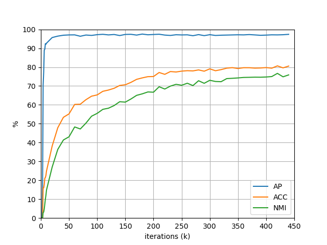
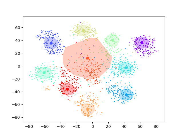
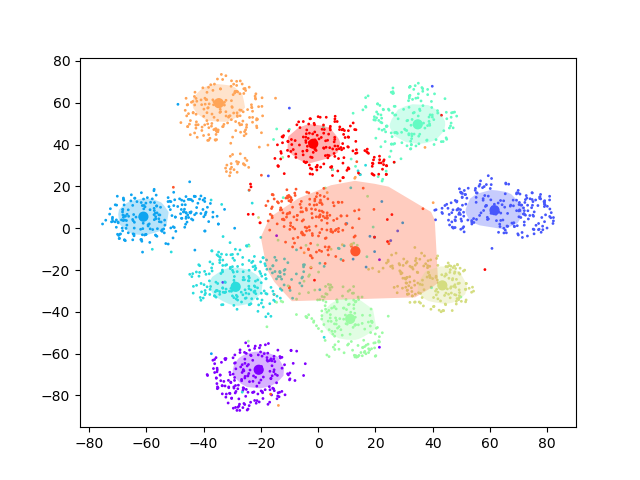
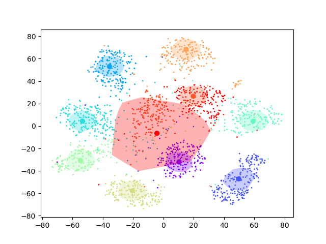
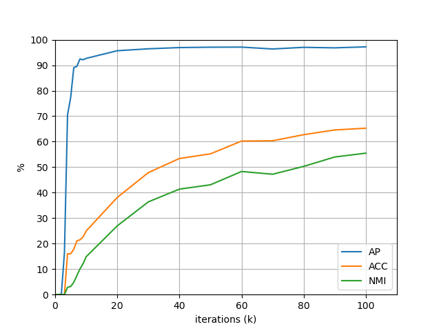
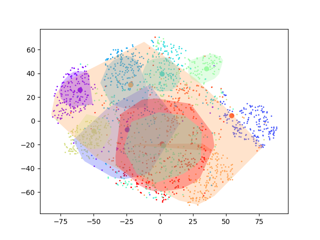
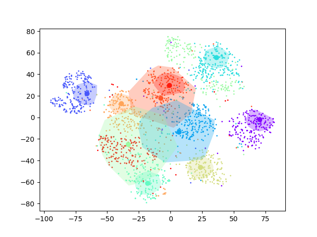
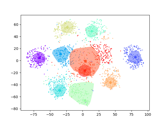
We conducted the experiments using the MultiMNIST dataset. We ran GMAIR for 440k iterations and observed the change in the values of the average precision (AP) of bounding boxes, accuracy (ACC), and normalized mutual information (NMI) of clustering until 100k iterations. We also visualized the “what” latent variables in the latent space during the process, as shown in Fig. 2. Although all values continued to increase even after 100k iterations, the visualization results were similar to those at the 100k iteration. For integrity, we reserved the results from 100k to 440k iterations in Appendix D. Details of calculating the AP, ACC, and NMI are discussed in Appendix C.

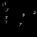
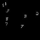
The results showed that at an early stage (~10k iterations) of training, models can already locate objects well with AP $>0.9$ (Fig. 2(a)). At the same time, $\mathbf{z}^{\mathsf{what}}$, representations of objects were still evolving, and the results of clustering (in Fig. 2(b)) was not desirable ((ACC, NMI) was ($0.24,0.15$)); the digits were a blur in Fig. 2(f). After 50k and 100k iterations of training, the clustering effect of $\mathbf{z}^{\mathsf{what}}$ was increasingly apparent, and the digits were clearer (Fig. 2(g), 2(h)). The clustering results ((ACC, NMI) was ($0.55,0.43$) at 50k, and ($0.65,0.55$) at 100k iterations) were improved (Fig. 2(c), 2(d)).

It should be noted that even if the clustering effect of $\mathbf{z}^{\mathsf{what}}$ is sufficiently enough, the model may fail to locate the centers of clusters (for example, the large cluster in light red in Fig. 2(d)), leading to poor clustering results. In the worst case, the model may learn to converge all $\mu_{k},\sigma_{k}(1\leq k\leq C)$ to the same values, $\mu^{*},\sigma^{*}$, and the Gaussian mixture model may degenerate to a single Gaussian distribution, $\mathcal{N}(\mu^{*},{\sigma^{*}}^{2})$, resulting in a miserable clustering result. In general, we found that this phenomenon usually occurs at the early stage of training and can be avoided by adjusting the learning rate of relative modules and the coefficients of the loss functions.

(a) AP(IoU=0.5), ACC and NMI during training

(b) “What” latent space, at 10k iterations

(c) “What” latent space, at 50k iterations

(d) “What” latent space, at 100k iterations

(e) Original image

(f) Generated image, at 10k iterations

(g) Generated image, at 50k iterations

(h) Generated image, at 100k iterations

Figure 2: “What” representation and cluster analysis. (a) Average precision (AP), accuracy (ACC), normalized mutual information (NMI) during training. (b-d) Visualized “what” latent space by t-SNE (Van der Maaten and Hinton (2008)) at 10k, 50k, and 100k iterations, respectively. Each small dot represents a sample of $\mathbf{z}^{\mathsf{what}}$, and different colors represent the ground-truth categories of the corresponding objects. The large dots are $\mu_{k}(1\leq k\leq C)$ described in Sec. 2.1, and each of these can be seen as the center of a cluster. The closures represent results of clustering, which are closures of the closest $n$ $\mathbf{z}^{\mathsf{what}}$ points to $\mu_{k}$ that are assigned to the $k$-th cluster (where $1\leq k\leq C$ and we choose $n=200$). The color of $\mu_{k}(1\leq k\leq C)$ and closures are decided by a matching algorithm such that a maximum number of $\mathbf{z}^{\mathsf{what}}$ are correctly classified to the ground-truth label. (e) Sample of original image. (f-h) Samples of generated image at 10k, 50k, and 100k iterations, respectively.

4.2 Image Generation

It is expected that $\mu_{k}(1\leq k\leq C)$ represents the average feature of the $k$-th type of objects, and $\mathbf{z}^{\mathsf{what}}_{i}$ latent variable can be decomposed into:

$$\mathbf{z}^{\mathsf{what}}_{i}=\mathbf{z}^{\mathsf{avg}}_{i}+\mathbf{z}^{\mathsf{local}}_{i}.$$ (12)

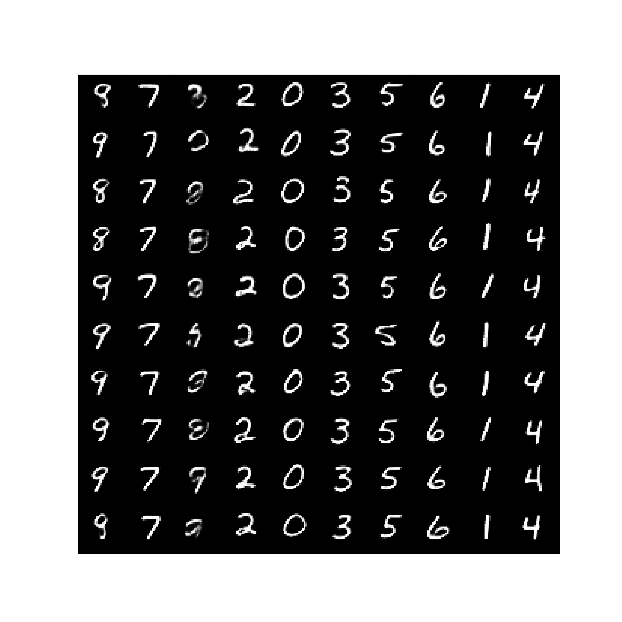
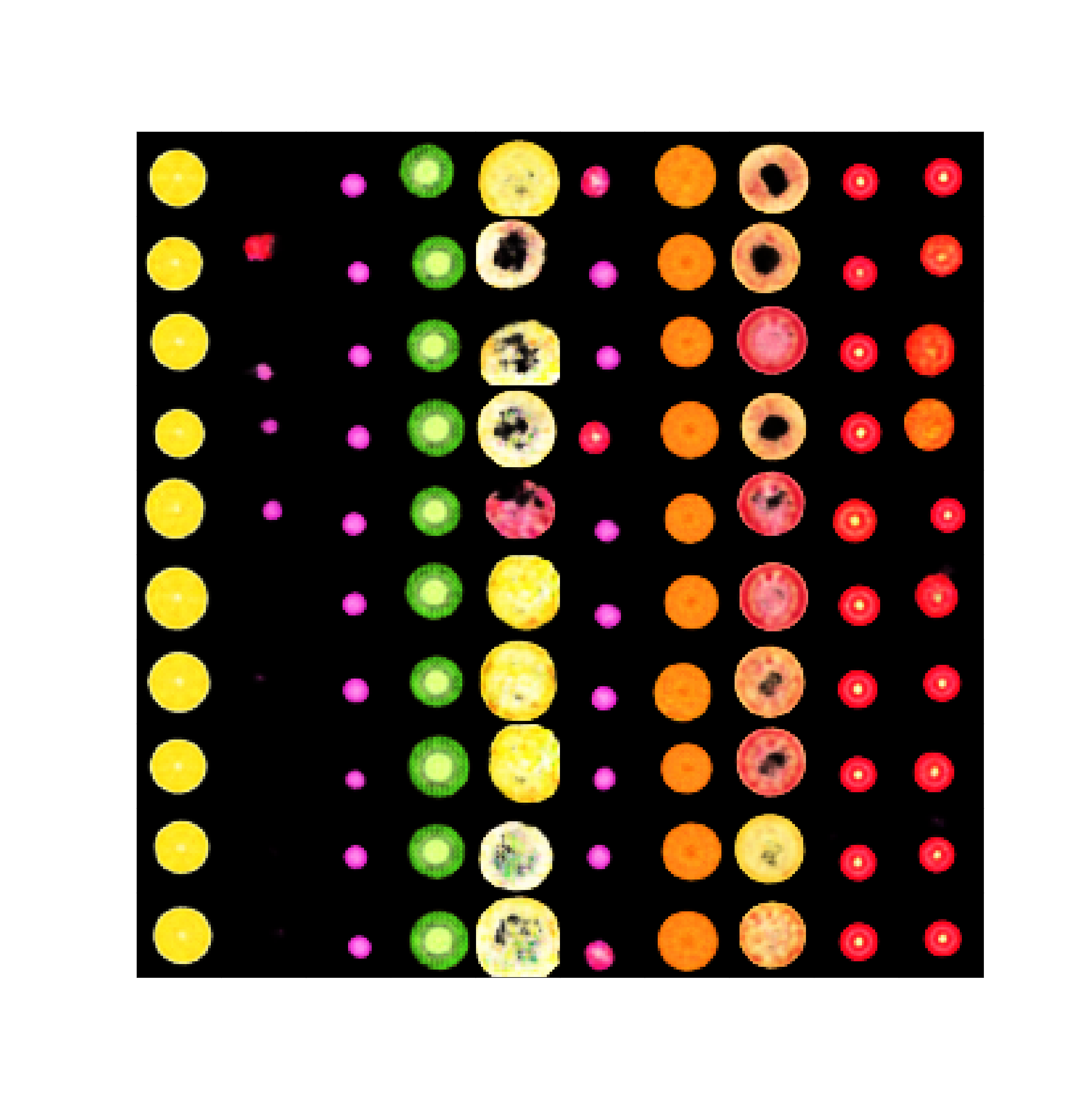
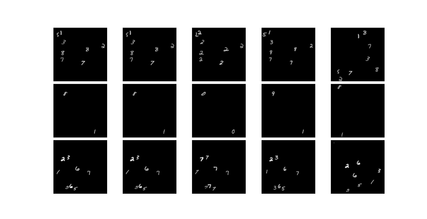
$\mathbf{z}^{\mathsf{avg}}_{i}=\mu_{k}(1\leq k\leq C)$ if the $i$-th object is in the $k$-th category and $\mathbf{z}^{\mathsf{local}}$ represents the local feature of the object. By altering $\mathbf{z}^{\mathsf{avg}}$ or $\mathbf{z}^{\mathsf{local}}$, we should obtain new objects that belong to other categories or the same category with different styles, respectively. In the experiment, we altered $\mathbf{z}^{\mathsf{avg}}$ and $\mathbf{z}^{\mathsf{local}}$ and observed the generated images for each object, as shown in Fig. 3. In Fig. 3(a), objects in each cluster correspond to a type of digit, which is exactly what we expected (except for digit 8 in column 3). In Fig. 3(b), categories with a large number of objects are grouped into multiple clusters, while categories with a small number are grouped into one cluster. This is due to the significant difference in number between various types. However, objects in a cluster come from a category in general.

The structure of GMAIR ensures its ability to control object categories, object styles, and the positions of each object of the generated images by altering $\mathbf{z}^{\mathsf{avg}}$, $\mathbf{z}^{\mathsf{local}}$, and $\mathbf{z}^{\mathsf{where}}$. Examples are shown in Fig. 4.

(a) MultiMNIST

(b) Fruit2D

Figure 3: Generated objects by varying $\mathbf{z}^{\mathsf{avg}}$ and $\mathbf{z}^{\mathsf{local}}$. The horizontal axis represents varying $\mathbf{z}^{\mathsf{avg}}$, and the vertical axis represents varying $\mathbf{z}^{\mathsf{local}}$, on both (a) and (b).

(a) MultiMNIST

(b) Fruit2D

Figure 4: Generated images by varying attributes and locations of objects. Columns 1 to 5 are numbered from left to right. Column 1 shows original images. Column 2 shows the generated images without varying $\mathbf{z}^{\mathsf{avg}}$, $\mathbf{z}^{\mathsf{local}}$, and $\mathbf{z}^{\mathsf{where}}$. Column 3 presents images generated by setting all $\mathbf{z}^{\mathsf{avg}}$ to the same random $\mu_{k}(1\leq k\leq C)$. Column 4 depicts images generated by varying $\mathbf{z}^{\mathsf{local}}$. Column 5 shows images generated by applying a random shuffle to $\mathbf{z}_{i}$.

This could provide a new approach for tasks such as style transfer, image generation, and data augmentation. Note that previous methods such as AIR, SPAIR, and its variants can also obtain similar results, but we achieve them in finer granularity.

4.3 Quantitative Evaluations

We quantitatively evaluate the models in terms of the AP of bounding boxes, ACC and NMI of the clusters, and the results are listed in Table 2. In the first part, we summarize some results of the state-of-the-art models for unsupervised clustering on MNIST dataset for comparison. In the second and the third part, we compare GMAIR to the state-of-the-art models for unsupervised object detection on MultiMNIST and Fruit2D dataset, respectively. The clustering results of SPAIR and SPACE are obtained by Gaussian mixture models (GMMs). Results show that GMAIR achieves competitive results on both clustering and localization.

Table 2: Quantitative Results on Localization (AP) and Clustering (Accuracy and NMI)

Model	Dataset	AP (%, IoU=0.5)	ACC (%)	NMI (%)
IIC	MNIST	—	$98.4\pm 0.652$	—
AAE (C=16)	MNIST	—	$90.45\pm 2.05$	—
AAE (C=30)	MNIST	—	$95.90\pm 1.13$	—
GMVAE (M=1)	MNIST	—	$77.78\pm 5.75$	—
GMVAE (M=10)	MNIST	—	$82.31\pm 3.75$	—
GMAIR	MultiMNIST	$97.3\pm 0.10$	$80.4\pm 0.48$	$75.5\pm 0.66$
SPAIR + GMM	MultiMNIST	$90.3$	$59.4\pm 1.50$	$56.3\pm 1.41$
SPACE + GMM	MultiMNIST	$96.7$	$68.8\pm 3.43$	$65.8\pm 2.85$
GMAIR	Fruit2D	$84.9\pm 1.56$	$90.9\pm 0.32$	$85.7\pm 1.25$
SPAIR + GMM	Fruit2D	$83.3$	$88.1\pm 0.70$	$78.4\pm 0.51$
SPACE + GMM	Fruit2D	$93.8$	$95.0\pm 1.99$	$87.0\pm 2.20$

5 Conclusion

We introduce GMAIR, which combines spatial attention and a Gaussian mixture, such that it can locate and cluster unseen objects simultaneously. We analyze the “what” latent variables and clustering process, provide examples of GMAIR application to the task of image generation, and evaluate GMAIR quantitatively compared with SPAIR and SPACE.

Appendix A Derivation of The KL Terms

In this section, we derive the KL terms in Eqn. 5. By assumption of $q(\mathbf{z}|\mathbf{x})$ and $p(\mathbf{z})$ (Eqn. 3 and Eqn. 1), we have:

$$\mathbb{E}_{q(\mathbf{z}|\mathbf{x})}\left[\log(\frac{q(\mathbf{z}|\mathbf{x})}{p(\mathbf{z})})\right]=\sum_{i=1}^{HW}\mathbb{E}_{q(\mathbf{z}_{i}|\mathbf{x})}\log\left(\frac{q(\mathbf{z}_{i}|\mathbf{x})}{p(\mathbf{z}_{i})}\right).$$ (13)

The term $\mathbb{E}_{q(\mathbf{z}_{i}|\mathbf{x})}\log\left(\frac{q(\mathbf{z}_{i}|\mathbf{x})}{p(\mathbf{z}_{i})}\right)$ can further be expanded as follow:

$$\mathbb{E}_{q(\mathbf{z}_{i}|\mathbf{x})}\log\left(\frac{q(\mathbf{z}_{i}|\mathbf{x})}{p(\mathbf{z}_{i})}\right)$$

$$= q(\mathbf{z}^{\mathsf{pres}}_{i}=0|\mathbf{x})\log\left(\frac{q(\mathbf{z}^{\mathsf{pres}}_{i}=0|\mathbf{x})}{p(\mathbf{z}^{\mathsf{pres}}_{i}=0)}\right)+q(\mathbf{z}^{\mathsf{pres}}_{i}=1|\mathbf{x})\left(\log\left(\frac{q(\mathbf{z}^{\mathsf{pres}}_{i}=1|\mathbf{x})}{p(\mathbf{z}^{\mathsf{pres}}_{i}=1)}\right)\right.$$

$$\left.+\mathbb{E}_{q(\mathbf{z}^{\mathsf{where}}_{i},\mathbf{z}^{\mathsf{depth}}_{i},\mathbf{z}^{\mathsf{cat}}_{i},\mathbf{z}^{\mathsf{what}}_{i}|\mathbf{x})}\left[\log\left(\frac{q(\mathbf{z}^{\mathsf{where}}_{i},\mathbf{z}^{\mathsf{depth}}_{i},\mathbf{z}^{\mathsf{cat}}_{i},\mathbf{z}^{\mathsf{what}}_{i}|\mathbf{x})}{p(\mathbf{z}^{\mathsf{where}}_{i},\mathbf{z}^{\mathsf{depth}}_{i},\mathbf{z}^{\mathsf{cat}}_{i},\mathbf{z}^{\mathsf{what}}_{i})}\right)\right]\right)$$ (14)

$$= KL\left(q(\mathbf{z}^{\mathsf{pres}}_{i}|\mathbf{x})||p(\mathbf{z}^{\mathsf{pres}}_{i})\right)$$

$$+q(\mathbf{z}^{\mathsf{pres}}_{i}=1|\mathbf{x})\mathbb{E}_{q(\mathbf{z}^{\mathsf{where}}_{i},\mathbf{z}^{\mathsf{depth}}_{i},\mathbf{z}^{\mathsf{cat}}_{i},\mathbf{z}^{\mathsf{what}}_{i}|\mathbf{x})}\left[\log\left(\frac{q(\mathbf{z}^{\mathsf{where}}_{i},\mathbf{z}^{\mathsf{depth}}_{i},\mathbf{z}^{\mathsf{cat}}_{i},\mathbf{z}^{\mathsf{what}}_{i}|\mathbf{x})}{p(\mathbf{z}^{\mathsf{where}}_{i},\mathbf{z}^{\mathsf{depth}}_{i},\mathbf{z}^{\mathsf{cat}}_{i},\mathbf{z}^{\mathsf{what}}_{i})}\right)\right].$$

Continue to expand Eqn. A:

$$\mathbb{E}_{q(\mathbf{z}^{\mathsf{where}}_{i},\mathbf{z}^{\mathsf{depth}}_{i},\mathbf{z}^{\mathsf{cat}}_{i},\mathbf{z}^{\mathsf{what}}_{i}|\mathbf{x})}\left[\log\left(\frac{q(\mathbf{z}^{\mathsf{where}}_{i},\mathbf{z}^{\mathsf{depth}}_{i},\mathbf{z}^{\mathsf{cat}}_{i},\mathbf{z}^{\mathsf{what}}_{i}|\mathbf{x})}{p(\mathbf{z}^{\mathsf{where}}_{i},\mathbf{z}^{\mathsf{depth}}_{i},\mathbf{z}^{\mathsf{cat}}_{i},\mathbf{z}^{\mathsf{what}}_{i})}\right)\right]$$

$$= \mathbb{E}_{q(\mathbf{z}^{\mathsf{where}}_{i}|\mathbf{x})}\log\left(\frac{q(\mathbf{z}^{\mathsf{where}}_{i}|\mathbf{x})}{p(\mathbf{z}^{\mathsf{where}}_{i})}\right)$$

$$+ \mathbb{E}_{q(\mathbf{z}^{\mathsf{depth}}_{i}|\mathbf{x})}\log\left(\frac{q(\mathbf{z}^{\mathsf{depth}}_{i}|\mathbf{x})}{p(\mathbf{z}^{\mathsf{depth}}_{i})}\right)$$ (15)

$$+ \mathbb{E}_{q(\mathbf{z}^{\mathsf{cat}}_{i},\mathbf{z}^{\mathsf{where}}_{i}|\mathbf{x})}\log\left(\frac{q(\mathbf{z}^{\mathsf{cat}}_{i}|\mathbf{x},\mathbf{z}^{\mathsf{where}})}{p(\mathbf{z}^{\mathsf{cat}}_{i})}\right)$$

$$+ \mathbb{E}_{q(\mathbf{z}^{\mathsf{what}}_{i},\mathbf{z}^{\mathsf{where}}_{i},\mathbf{z}^{\mathsf{cat}}_{i}|\mathbf{x})}\log\left(\frac{q(\mathbf{z}^{\mathsf{what}}_{i}|\mathbf{x},\mathbf{z}^{\mathsf{where}},\mathbf{z}^{\mathsf{cat}}_{i})}{p(\mathbf{z}^{\mathsf{what}}_{i}|\mathbf{z}^{\mathsf{cat}}_{i})}\right).$$

By the definition of Kullback–Leibler divergence, the four terms in the RHS of Eqn. A are indeed

$$KL\left(q(\mathbf{z}^{\mathsf{where}}_{i}|\mathbf{x})||p(\mathbf{z}^{\mathsf{where}}_{i})\right),$$

$$KL\left(q(\mathbf{z}^{\mathsf{depth}}_{i}|\mathbf{x})||p(\mathbf{z}^{\mathsf{depth}}_{i})\right),$$

$$\mathbb{E}_{q(\mathbf{z}^{\mathsf{where}}_{i}|\mathbf{x})}\left[KL\left(q(\mathbf{z}^{\mathsf{cat}}_{i}|\mathbf{x},\mathbf{z}^{\mathsf{where}}_{i})||p(\mathbf{z}^{\mathsf{cat}}_{i})\right)\right],$$

and $$\mathbb{E}_{q(\mathbf{z}^{\mathsf{where}}_{i},\mathbf{z}^{\mathsf{cat}}_{i}|\mathbf{x})}\left[KL\left(q(\mathbf{z}^{\mathsf{what}}_{i}|\mathbf{x},\mathbf{z}^{\mathsf{where}}_{i},\mathbf{z}^{\mathsf{cat}}_{i})||p(\mathbf{z}^{\mathsf{what}}_{i}|\mathbf{z}^{\mathsf{cat}}_{i})\right)\right],$$

respectively. Therefore, we complete the proof of Eqn. 5.

During the implementation, we model discrete variables $\mathbf{z}^{\mathsf{pres}}$ and $\mathbf{z}^{\mathsf{cat}}$ using the Gumbel-Softmax approximation (Jang et al. (2016)). Therefore, all variables are differentiable using the reparameterization trick.

Appendix B Implementation Details

Our code is available at https://github.com/EmoFuncs/GMAIR-pytorch.

B.1 Models

Here, we describe the architecture of each module of GMAIR, as shown in Fig. 1. The backbone is a ResNet18 (He et al. (2016)) network with two deconvolution layers replacing the fully connected layer, as shown in Table 3. Pres-head, depth-head, and where-head are convolutional networks that are only different from the number of output channels, as shown in Table 4. What-encoder and cat-encoder are multiple layer networks, as shown in Table 5. Finally, the glimpse decoder is a deconvolutional network, as shown in Table 6.

For other models, we make use of code from https://github.com/yonkshi/SPAIR_pytorch for SPAIR, and https://github.com/zhixuan-lin/SPACE for SPACE. We utilize most of the default configuration for both models, and only change $A$ (the dimension of $\mathbf{z}^{\mathsf{what}}_{i}$) to $256$ for comparison, the size of the base bounding box to $72\times 72$ for large objects.

B.2 Training and Hyperparameters

The base set of hyperparameters for GMAIR is given in Table 7. The value $p$ (the prior on $\mathbf{z}^{\mathsf{pres}}$) drops gradually from $1$ to the final value $6\mbox{e-}6$, and the value $\alpha_{\mathsf{overlap}}$ drops from $2$ to $0$ in the early stage of training for stability. The learning rate is in the range of $[5\mbox{e-}5,1\mbox{e-}4]$.

B.3 Testing

During testing phase, in order to obtain deterministic results, we use the value with the largest probability (density) for latent variables $\mathbf{z}$, instead of sampling them from the distributions. To be specific, we use $\boldsymbol{\pi},\mu^{\mathsf{depth}},p,\mu^{\mathsf{what}},\mbox{ and }\mu^{\mathsf{where}}$ for $\mathbf{z}^{\mathsf{cat}},\mathbf{z}^{\mathsf{depth}},\mathbf{z}^{\mathsf{pres}},\mathbf{z}^{\mathsf{what}}$ and $\mathbf{z}^{\mathsf{where}}$, respectively.

Appendix C Calculation of AP, ACC and NMI

The value of AP is calculated at threshold $\mbox{IoU}=0.5$ by using the calculation method from the VOC (Everingham et al. (2010)). Before calculating the ACC and NMI of clusters, we filter the incorrect bounding boxes. A predicted box $PB$ is correct iff there is a ground-truth box $GB$ such that $\operatorname{IoU}(PB,GB)>0.5$, and the class of a correct predicted box $PB$ is assigned to the class of the ground-truth box $GB$ such that $\operatorname{IoU}(PB,GB)$ is maximized. After filtering, all correct predicted boxes are used for the calculation of ACC and NMI. Note that we still have many ways to assign each predicted category to a real category when calculating the value of ACC. In all of the ways, we select the one such that ACC is maximized, following Dilokthanakul et al. (2016). Formulas are shown in Eqn. 16 and Eqn. 17 for the calculation of ACC and NMI:

$$\mbox{ACC}=\frac{\sum_{k=1}^{C}\max_{1\leq j\leq C^{\prime}}|\left\{i|G_{i}=j,P_{i}=k\right\}|}{|P|}$$ (16)

$$\mbox{NMI}=\frac{2I(G,P)}{H(G)+H(P)}$$ (17)

where $G$ and $P$ are respectively the ground-truth categories and predicted categories for all correct boxes, $C$ and $C^{\prime}$ are the number of clusters and real classes, $H(\cdot)$ and $I(\cdot,\cdot)$ are the entropy and mutual information function, respectively.

Table 3: Architecture of Backbone

Layer	Type	Size	Act./Norm.	Output Size
resnet	ResNet18 (w/o fc)			$512\times 4\times 4$
deconv layer 1	Deconv	$128$	ReLU/BN	$128\times 8\times 8$
deconv layer 2	Deconv	$64$	ReLU/BN	$64\times 16\times 16$

Table 4: Architectures of Pres/Depth/Where-Head

Layer	Type	Size	Act./Norm.	Output Size
Input				$64\times 16\times 16$
Hidden	Conv	$\left[3\times 3,128\right]\times 3$	ReLU	$128\times 16\times 16$
Output	Conv	$1\times 1,1/1/4$		$1/1/4\times 16\times 16$

Table 5: Architectures of What/Cat-Encoder

Layer	Type	Size	Act./Norm.	Output Size
Input	Flatten			$(3\times 32\times 32=)3072$
Layer 1	Linear	$3072\times 128$	ReLU	$128$
Layer 2	Linear	$128\times 256$	ReLU	$256$
Layer 3	Linear	$256\times 512$	ReLU	$512$
Output	Linear	$512\times A/C$		$A/C$

Table 6: Architecture of Glimpse-Decoder

Layer	Type	Size	Act./Norm.	Output Size
Input	Linear	$A\times 256$	ReLU	$256\times 1\times 1$
Layer 1	Deconv	$128$	ReLU/GN(8)	$128\times 2\times 2$
Layer 2	Deconv	$128$	ReLU/GN(8)	$128\times 4\times 4$
Layer 3	Deconv	$64$	ReLU/GN(8)	$64\times 8\times 8$
Layer 4	Deconv	$32$	ReLU/GN(8)	$32\times 16\times 16$
Conv	Conv	$3\times 3,32$	ReLU/GN(8)	$32\times 16\times 16$
Layer 5	DeConv	$16$	ReLU/GN(4)	$16\times 32\times 32$
Output	Conv	$3\times 3,3$		$3\times 32\times 32$

Table 7: Base Hyperparameters

Description	Variable	Value
Base bbox size	$(a_{h},a_{w})$	$(72,72)$
Batch size		$16$
Dim. of $\mathbf{z}^{\mathsf{what}}_{i}$	$A$	$256$
Dim. of $\mathbf{z}^{\mathsf{cat}}_{i}$	$C$	$10$
Glimpse size	$(H_{obj},W_{obj})$	$(32,32)$
Learning rate		$[5\mbox{e-}5,1\mbox{e-}4]$
Loss Coef. of $L_{\mathsf{cat}}$	$\alpha_{\mathsf{cat}}$	1
Loss Coef. of $L_{\mathsf{overlap}}$	$\alpha_{\mathsf{overlap}}$	$2\rightarrow 0$
Loss Coef. of $L_{\mathsf{depth}}$	$\alpha_{\mathsf{depth}}$	1
Loss Coef. of $L_{\mathsf{pres}}$	$\alpha_{\mathsf{pres}}$	1
Loss Coef. of $L_{\mathsf{recon}}$	$\alpha_{\mathsf{recon}}$	8,16
Loss Coef. of $L_{\mathsf{what}}$	$\alpha_{\mathsf{recon}}$	1
Loss Coef. of $L_{\mathsf{where}}$	$\alpha_{\mathsf{recon}}$	1
Prior on $\mathbf{z}^{\mathsf{cat}}$	$\boldsymbol{\pi}$	$(1/C,...,1/C)$
Prior on $\mathbf{z}^{\mathsf{depth}}$	$(\mu^{\mathsf{depth}}_{\mathsf{prior}},{\sigma^{\mathsf{depth}}_{\mathsf{prior}}})$	$(0,1)$
Prior on $\mathbf{z}^{\mathsf{pres}}$	$p$	$1\rightarrow 6\mbox{e-}6$
Prior on $\mathbf{z}^{\mathsf{where}}$	$(\mu^{\mathsf{where}}_{\mathsf{prior}},{\sigma^{\mathsf{where}}_{\mathsf{prior}}})$	$(0,1)$
Prior on $\mathbf{z}^{\mathsf{what}}$	$(\mu^{\mathsf{what}}_{\mathsf{prior}},{\sigma^{\mathsf{what}}_{\mathsf{prior}}})$	$(0,1)$

Appendix D Additional Experiment Results

The graphs of “what” representation after 100k iterations are shown in Fig. 5.

(a) AP(IoU=0.5), ACC and NMI during training

(b) “What” latent space, at 220k iterations

(c) “What” latent space, at 330k iterations

(d) “What” latent space, at 440k iterations

(e) Original image

(f) Generated image, at 220k iterations

(g) Generated image, at 330k iterations

(h) Generated image, at 440k iterations

Figure 5: “What” representation and cluster analysis after 100k iterations. (a) Average precision (AP), accuracy (ACC), normalized mutual information (NMI) during training. (b-d) Visualized “what” latent space by t-SNE (Van der Maaten and Hinton (2008)) at 220k, 330k, and 440k iterations, respectively. (e) Sample of original image. (f-h) Samples of generated image at 220k, 330k, and 440k iterations, respectively.

References

- Burgess et al. (2019) C. P. Burgess, L. Matthey, N. Watters, R. Kabra, I. Higgins, M. Botvinick, and A. Lerchner. Monet: Unsupervised scene decomposition and representation. arXiv preprint arXiv:1901.11390, 2019.
- Charakorn et al. (2020) R. Charakorn, Y. Thawornwattana, S. Itthipuripat, N. Pawlowski, P. Manoonpong, and N. Dilokthanakul. An explicit local and global representation disentanglement framework with applications in deep clustering and unsupervised object detection. arXiv preprint arXiv:2001.08957, 2020.
- Crawford and Pineau (2019) E. Crawford and J. Pineau. Spatially invariant unsupervised object detection with convolutional neural networks. In Proceedings of the AAAI Conference on Artificial Intelligence, volume 33, pages 3412–3420, 2019.
- Crawford and Pineau (2020) E. Crawford and J. Pineau. Exploiting spatial invariance for scalable unsupervised object tracking. In Proceedings of the AAAI Conference on Artificial Intelligence, volume 34, pages 3684–3692, 2020.
- Dilokthanakul et al. (2016) N. Dilokthanakul, P. A. Mediano, M. Garnelo, M. C. Lee, H. Salimbeni, K. Arulkumaran, and M. Shanahan. Deep unsupervised clustering with gaussian mixture variational autoencoders. arXiv preprint arXiv:1611.02648, 2016.
- Duan et al. (2019) K. Duan, S. Bai, L. Xie, H. Qi, Q. Huang, and Q. Tian. Centernet: Keypoint triplets for object detection. In Proceedings of the IEEE/CVF International Conference on Computer Vision, pages 6569–6578, 2019.
- Engelcke et al. (2019) M. Engelcke, A. R. Kosiorek, O. P. Jones, and I. Posner. Genesis: Generative scene inference and sampling with object-centric latent representations. arXiv preprint arXiv:1907.13052, 2019.
- Eslami et al. (2016) S. Eslami, N. Heess, T. Weber, Y. Tassa, D. Szepesvari, K. Kavukcuoglu, and G. E. Hinton. Attend, infer, repeat: Fast scene understanding with generative models. arXiv preprint arXiv:1603.08575, 2016.
- Everingham et al. (2010) M. Everingham, L. Van Gool, C. K. Williams, J. Winn, and A. Zisserman. The pascal visual object classes (voc) challenge. International journal of computer vision, 88(2):303–338, 2010.
- Greff et al. (2017) K. Greff, S. Van Steenkiste, and J. Schmidhuber. Neural expectation maximization. arXiv preprint arXiv:1708.03498, 2017.
- Greff et al. (2019) K. Greff, R. L. Kaufman, R. Kabra, N. Watters, C. Burgess, D. Zoran, L. Matthey, M. Botvinick, and A. Lerchner. Multi-object representation learning with iterative variational inference. In International Conference on Machine Learning, pages 2424–2433. PMLR, 2019.
- Gu et al. (2021) C. Gu, H. Xie, X. Lu, and C. Zhang. Cgmvae: Coupling gmm prior and gmm estimator for unsupervised clustering and disentanglement. IEEE Access, 2021.
- He et al. (2016) K. He, X. Zhang, S. Ren, and J. Sun. Identity mappings in deep residual networks. In European conference on computer vision, pages 630–645. Springer, 2016.
- Higgins et al. (2016) I. Higgins, L. Matthey, A. Pal, C. Burgess, X. Glorot, M. Botvinick, S. Mohamed, and A. Lerchner. beta-vae: Learning basic visual concepts with a constrained variational framework. 2016.
- Ioffe and Szegedy (2015) S. Ioffe and C. Szegedy. Batch normalization: Accelerating deep network training by reducing internal covariate shift. In International conference on machine learning, pages 448–456. PMLR, 2015.
- Jaderberg et al. (2015) M. Jaderberg, K. Simonyan, A. Zisserman, and K. Kavukcuoglu. Spatial transformer networks. arXiv preprint arXiv:1506.02025, 2015.
- Jang et al. (2016) E. Jang, S. Gu, and B. Poole. Categorical reparameterization with gumbel-softmax. arXiv preprint arXiv:1611.01144, 2016.
- Ji et al. (2019) X. Ji, J. F. Henriques, and A. Vedaldi. Invariant information clustering for unsupervised image classification and segmentation. In Proceedings of the IEEE/CVF International Conference on Computer Vision, pages 9865–9874, 2019.
- Kingma and Welling (2013) D. P. Kingma and M. Welling. Auto-encoding variational bayes. arXiv preprint arXiv:1312.6114, 2013.
- Kosiorek et al. (2018) A. R. Kosiorek, H. Kim, I. Posner, and Y. W. Teh. Sequential attend, infer, repeat: Generative modelling of moving objects. arXiv preprint arXiv:1806.01794, 2018.
- LeCun (1998) Y. LeCun. The mnist database of handwritten digits. http://yann.lecun.com/exdb/mnist/, 1998.
- LeCun et al. (1998) Y. LeCun, L. Bottou, Y. Bengio, and P. Haffner. Gradient-based learning applied to document recognition. Proceedings of the IEEE, 86(11):2278–2324, 1998.
- Lin et al. (2020) Z. Lin, Y.-F. Wu, S. V. Peri, W. Sun, G. Singh, F. Deng, J. Jiang, and S. Ahn. Space: Unsupervised object-oriented scene representation via spatial attention and decomposition. arXiv preprint arXiv:2001.02407, 2020.
- Liu et al. (2016) W. Liu, D. Anguelov, D. Erhan, C. Szegedy, S. Reed, C.-Y. Fu, and A. C. Berg. Ssd: Single shot multibox detector. In European conference on computer vision, pages 21–37. Springer, 2016.
- Loper and Black (2014) M. M. Loper and M. J. Black. Opendr: An approximate differentiable renderer. In European Conference on Computer Vision, pages 154–169. Springer, 2014.
- Makhzani et al. (2015) A. Makhzani, J. Shlens, N. Jaitly, I. Goodfellow, and B. Frey. Adversarial autoencoders. arXiv preprint arXiv:1511.05644, 2015.
- Redmon et al. (2016) J. Redmon, S. Divvala, R. Girshick, and A. Farhadi. You only look once: Unified, real-time object detection. In Proceedings of the IEEE conference on computer vision and pattern recognition, pages 779–788, 2016.
- Springenberg (2015) J. T. Springenberg. Unsupervised and semi-supervised learning with categorical generative adversarial networks. arXiv preprint arXiv:1511.06390, 2015.
- Stelzner et al. (2019) K. Stelzner, R. Peharz, and K. Kersting. Faster attend-infer-repeat with tractable probabilistic models. In International Conference on Machine Learning, pages 5966–5975. PMLR, 2019.
- Sun (2019) S.-H. Sun. Multi-digit mnist for few-shot learning, 2019. URL https://github.com/shaohua0116/MultiDigitMNIST.
- Van der Maaten and Hinton (2008) L. Van der Maaten and G. Hinton. Visualizing data using t-sne. Journal of machine learning research, 9(11), 2008.
- Wang et al. (2019) D. Wang, M. Jamnik, and P. Lio. Unsupervised and interpretable scene discovery with discrete-attend-infer-repeat. arXiv preprint arXiv:1903.06581, 2019.
- Wu and He (2018) Y. Wu and K. He. Group normalization. In Proceedings of the European conference on computer vision (ECCV), pages 3–19, 2018.
- Zhu et al. (2020) Q. Zhu, J. Su, W. Bi, X. Liu, X. Ma, X. Li, and D. Wu. A batch normalized inference network keeps the kl vanishing away. arXiv preprint arXiv:2004.12585, 2020.